fMRI and visual brain function

Dr. Tessa DekkerUCL Institute of Ophthalmology

6th February 2018

Brief history of brain imaging

• 1895 – First human X-ray image

• 1950 – First human PET scan - uses traces of IV radioactive material

(carbon, nitrogen, fluorine or oxygen) to map neural activity

• 1977 – First human MRI scan

• 1991 – First fMRI paper published

In 1992 only 4 published articles using fMRI

In 2011 ‘fMRI’ search returns over 32,000 peer-reviewed articles

this morning over 415,010 peer-reviewed articles on PubMed

Why ? Non-invasive and has excellent spatial resolution

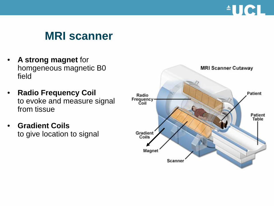
• A strong magnet forhomgeneous magnetic B0 field

• Radio Frequency Coilto evoke and measure signal from tissue

• Gradient Coilsto give location to signal

MRI scanner

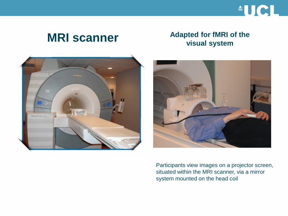
MRI scanner Adapted for fMRI of the visual system

Participants view images on a projector screen, situated within the MRI scanner, via a mirror system mounted on the head coil

Brief overview of standard MRI

• The MRI scanner houses a very large super-cooled electro-magnet

• Research magnets typically have a strength of 3Tesla: ~ 50,000x the earth’s magnetic field

• MRI utilises the property of hydrogen atoms in each of the molecules of water in our body – each is a tiny magnetic dipole (+ve proton nucleus and a single orbiting –ve electron)

• Normally these atomic nuclei are randomly oriented, but when placed within a very strong magnetic field, they become aligned with the direction of the magnetic field

• A short pulse of radio frequency (RF) energy perturbs these tiny magnets from their preferred alignment, and as they subsequently return to their original position they emit small amounts of energy that are large enough to measure

• Different brain tissues have different amounts of water, and hence produce different intensities of signal that can be used to differentiate between them, e.g. white matter has a higher concentration of water than grey matter and therefore emits a different signal intensity

Gradients

• Add magnetic gradients on top of B0

• Used to create slices and voxels in the space from where the RF signal is measured

voxels slices volume

How does fMRI work?

• fMRI measures changes in blood oxygenation that occur in response to a neural event

• Oxyhaemoglobin (HbO2) is diamagnetic (weakly magnetic), but deoxyhaemoglobin (HbR) is paramagnetic (strong magnetic moment)

• Therefore red blood cells containing deoxyhaemoglobin cause distortion to the magnetic field and lower the MR signal compared to fully oxygenated blood

• Since blood oxygenation varies depending on the level of neuronal activity, these differences can be used to detect brain activity

• This form of MRI is referred to as ‘blood oxygenation level dependent’, or BOLD imaging

• It is this BOLD signal that is reported in fMRI studies

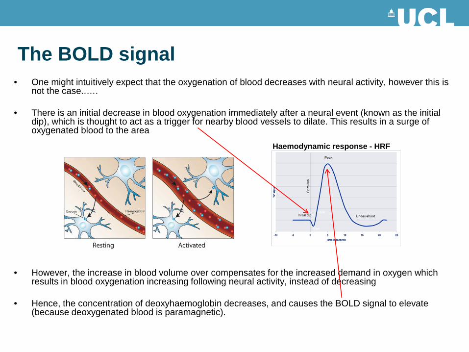
• One might intuitively expect that the oxygenation of blood decreases with neural activity, however this is not the case..….

• There is an initial decrease in blood oxygenation immediately after a neural event (known as the initial dip), which is thought to act as a trigger for nearby blood vessels to dilate. This results in a surge of oxygenated blood to the area

• However, the increase in blood volume over compensates for the increased demand in oxygen which results in blood oxygenation increasing following neural activity, instead of decreasing

• Hence, the concentration of deoxyhaemoglobin decreases, and causes the BOLD signal to elevate (because deoxygenated blood is paramagnetic).

The BOLD signal

Haemodynamic response - HRF

How does the BOLD signal relate to neural activity?

• A high-resolution neuroimaging ‘voxel’ (1x1x1mm) has ~50,000 neurons

• BOLD signal follows the HRF which peaks at around 4-6 seconds post stimulus onset

• So what is the BOLD signal really telling us about neural activity?

Logothetis and colleagues (2001), simultaneously recorded single and multi-unit spiking activity, as well as local field potentials (LFPs) and BOLD contrast in monkeys, and showed that the BOLD signal correlated best with local field potentials (LFPs) rather than the spiking activity

However similar research in humans (on epileptic patients with implanted electrodes) found equally good correlations between spikes and BOLD as between LFPs and BOLD (Mukamel et al. 2005)

Thus, it remains debated whether the BOLD signal reflects input to neurons (as reflected in the LFPs), or the output from neurons (reflected by their spiking activity)

• Refs:‘What we can do and what we cannot do with fMRI’, N.K. Logothetis, nature 453, 869-878, 2008‘Interpreting the BOLD signal’, N.K. Logethetis & B.A. Wandell, Annual Rev of Physiology, 66:735-769

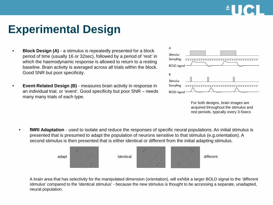
• Block Design (A) - a stimulus is repeatedly presented for a block period of time (usually 16 or 32sec), followed by a period of ‘rest’ in which the haemodynamic response is allowed to return to a resting baseline. Brain activity is averaged across all trials within the block. Good SNR but poor specificity.

• Event-Related Design (B) - measures brain activity in response in an individual trial, or ‘event’. Good specificity but poor SNR – needs many many trials of each type.

Experimental Design

For both designs, brain images are acquired throughout the stimulus and rest periods, typically every 3-5secs

• fMRI Adaptation - used to isolate and reduce the responses of specific neural populations. An initial stimulus is presented that is presumed to adapt the population of neurons sensitive to that stimulus (e.g.orientation). A second stimulus is then presented that is either identical or different from the initial adapting stimulus.

A brain area that has selectivity for the manipulated dimension (orientation), will exhibit a larger BOLD signal to the ‘different stimulus’ compared to the ‘identical stimulus’ - because the new stimulus is thought to be accessing a separate, unadapted, neural population.

adapt identical different

– Activation maps represent the ‘activity’ in each unit of the brain (voxel), i.e. the response of a population of neurons.

– ‘Activity’ is defined by how closely the time-course of the BOLD signal matches that of the visual stimulus.

– Those voxels that show tight correspondance with the stimulus are given a high activation score, voxels showing no correlation are given a low or zero score and those showing the opposite correlation (i.e. deactivations) are given a negative score.

Activation maps

Activation map

Multi-slice acquisition

~30 slices at 2mm slice thickness

~ 3 sec to acquire all 20 slices

Model the time series

movie clip

Functionally localising the cortical visual areasV1-V3

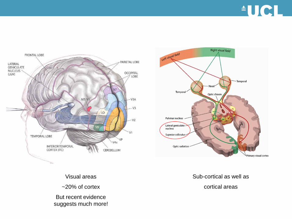
Visual areas

~20% of cortex

But recent evidence suggests much more!

Sub-cortical as well as

cortical areas

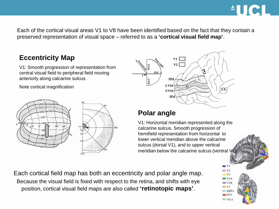
Each of the cortical visual areas V1 to V8 have been identified based on the fact that they contain a preserved representation of visual space – referred to as a ‘cortical visual field map’.

Eccentricity MapV1: Smooth progression of representation from central visual field to peripheral field moving anteriorly along calcarine sulcus.

Note cortical magnification

Each cortical field map has both an eccentricity and polar angle map.Because the visual field is fixed with respect to the retina, and shifts with eye

position, cortical visual field maps are also called ‘retinotopic maps’.

Polar angleV1: Horizontal meridian represented along the calcarine sulcus. Smooth progression of hemifield representation from horizontal to lower vertical meridian above the calcarine sulcus (dorsal V1), and to upper vertical meridian below the calcarine sulcus (ventral V1).

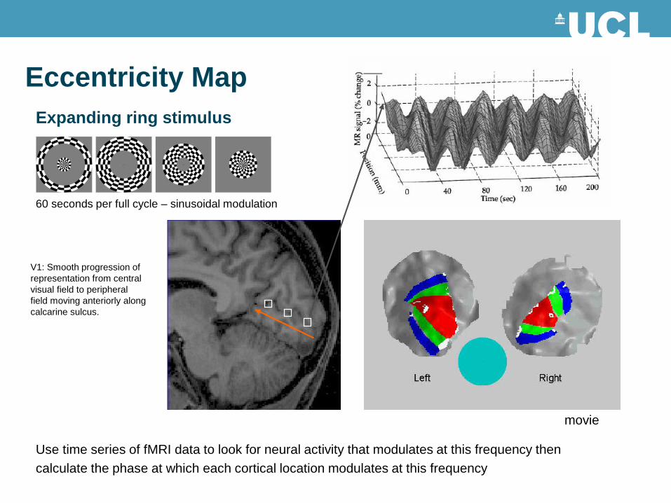
Eccentricity MapExpanding ring stimulus

Use time series of fMRI data to look for neural activity that modulates at this frequency then calculate the phase at which each cortical location modulates at this frequency

60 seconds per full cycle – sinusoidal modulation

V1: Smooth progression of representation from central visual field to peripheral field moving anteriorly along calcarine sulcus.

movie

Polar AngleRotating Wedge stimulus

60 seconds per full cycle – sinusoidal modulation

Use time series of fMRI data to look for neural activity that modulates at this frequency then calculate the phase at which each cortical location modulates at this frequency

V1: Horizontal meridian represented along the calcarine sulcus. Smooth progression of hemifield representation from horizontal to lower vertical meridian above the calcarine sulcus (dorsal V1), and to upper vertical meridian below the calcarine sulcus (ventral V1).

movie

Fourier Transform

Complex data(amplitude, phase)

Fourier Analysis

Fourier analysis of the fMRI time series at stimulus frequency --> amplitude, phaseAmplitude - strength of retinotopyPhase - spatial locationResults plotted on cortical surface

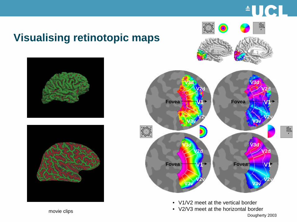
Visualising retinotopic maps

movie clips

V2d

V2d

Fovea

Fovea Fovea

Fovea

V2v

V2v

V2v

V2v

V2d V2d

V2dV2d

V3v

V3d

V3v

V3v V3v

V3d

V3dV3d

V1

V1

V1

V1

• V1/V2 meet at the vertical border • V2/V3 meet at the horizontal border

Dougherty 2003

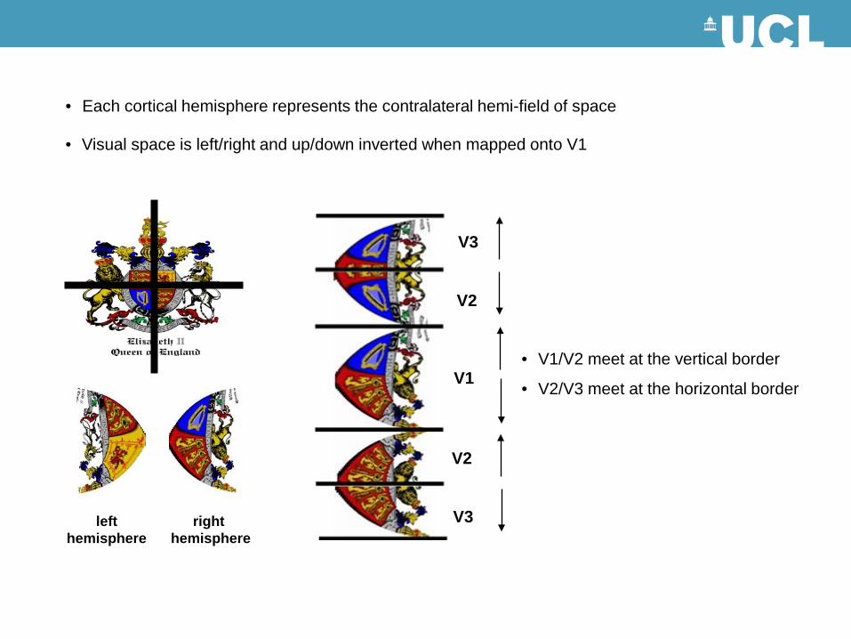
• Each cortical hemisphere represents the contralateral hemi-field of space

• Visual space is left/right and up/down inverted when mapped onto V1

• V1/V2 meet at the vertical border

• V2/V3 meet at the horizontal borderV1

V2

V3

V2

V3right hemisphere

lefthemisphere

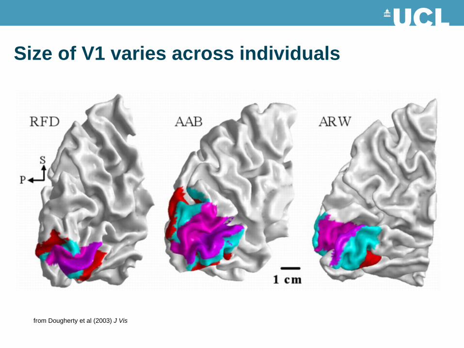
Size of V1 varies across individuals

from Dougherty et al (2003) J Vis

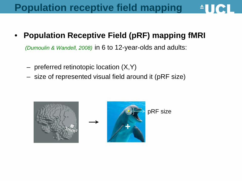
• Population Receptive Field (pRF) mapping fMRI (Dumoulin & Wandell, 2008) in 6 to 12-year-olds and adults:

– preferred retinotopic location (X,Y) – size of represented visual field around it (pRF size)

+pRF size

Population receptive field mapping

Population receptive field mapping

wedge: 1. polar angle map

Stimulus viewed by subjects in scanner

ring: 2. eccentricity map

29.7°

used to draw ROI

V1-V3

plot eccentricity against pRF

Method

3. population receptive field size

4 runs x144

volumes

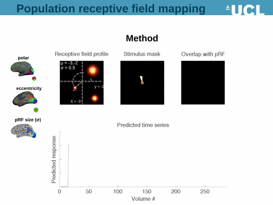
μ = -3,-2σ = 0.5

polar

eccentricity

polar

Method

X = -3

y = -2

pRF size (σ)

Population receptive field mapping

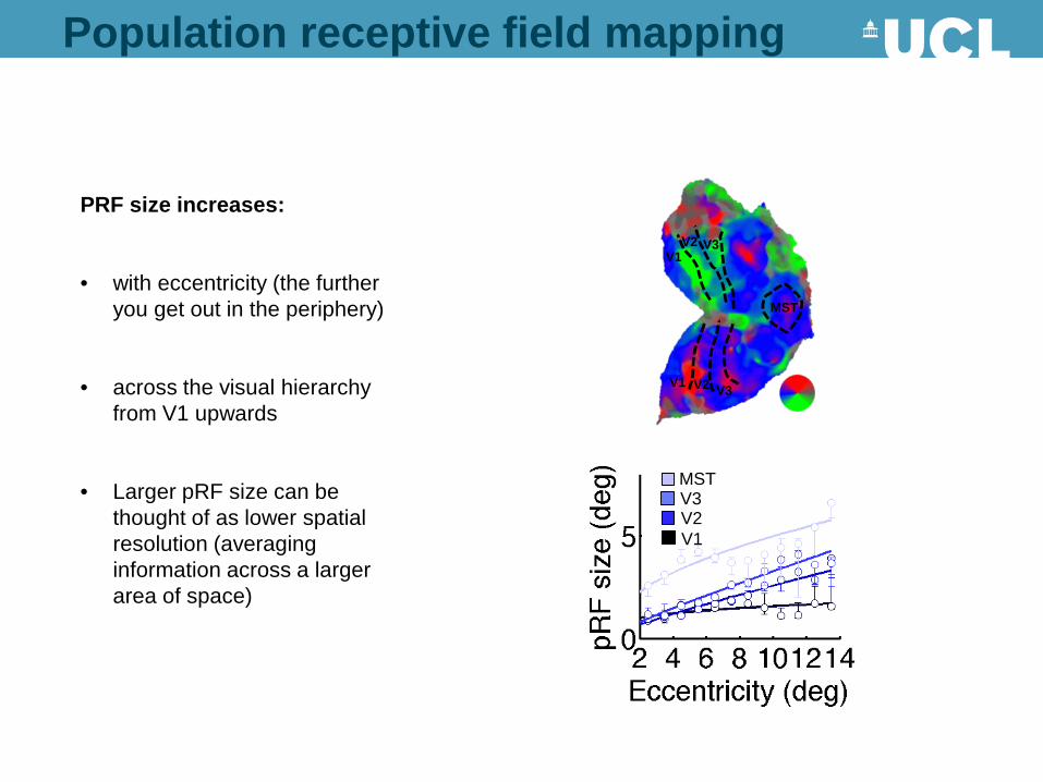
V1V2 V3

V1 V2 V3

MST

PRF size increases:

• with eccentricity (the further you get out in the periphery)

• across the visual hierarchy from V1 upwards

• Larger pRF size can be thought of as lower spatial resolution (averaging information across a larger area of space)

V1V2V3MST

Population receptive field mapping

Pre-play of visual stimuli in V1Ekman, Kok & de Lange (2017). Nature Communications

Population receptive field mapping

Functionally localising the sub-cortical visual areas

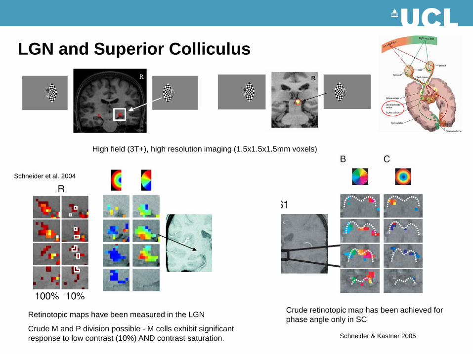
High field (3T+), high resolution imaging (1.5x1.5x1.5mm voxels)

Retinotopic maps have been measured in the LGN

Crude M and P division possible - M cells exhibit significant response to low contrast (10%) AND contrast saturation.

LGN and Superior Colliculus

Schneider et al. 2004

Schneider & Kastner 2005

Crude retinotopic map has been achieved for phase angle only in SC

Why do we want to measure visual field maps?

1. There are no anatomical landmarks that can be used to delineate the different visual areas.

2. Different visual regions are specialised for different perceptual functions, characterising the responses within a specific visual field map is essential for understanding cortical organisation of visual functions, and for understanding the implications of localised lesions.

3. Much of our knowledge about the human brain has been derived from non-human primates, but differences between human and non-human primates make direct measurements essential.

4. Quantitative measurements of visual field maps can be used for detailed analyses of visual system pathologies, e.g. for tracking changes in cortical organisation following retinal or cortical injury (plasticity) and more recently for assessing the benefits of gene- & stem-cell based therapy for inherited retinal disease

5. When making conclusions about visual responses within an individual on separate occasions, or between individuals within a group, it is essential to know that the same functional area is being compared. Anatomical markers alone are not reliable due to individual variability in anatomy.

Characterising responses within retinotopically defined areas

Consistency of characteristics within V1-V3

• V1-V3 share a foveal confluence and their eccentricity maps run in register

• Consistency across individuals / laboratories on the way visual space is represented within V1–V3

• Hierarchy of responses

• V1 – orientation, spatial frequency, contrast, colour coding, motion sensitive, ocular dominance columns

• V2 – more complex pattern analysis, illusory contours, crowding

• V3 – colour selective, global motion

• A lesion to these areas usually results in a general loss of visual function within the corresponding area of visual field

V2d

V2d

Fovea

Fovea Fovea

Fovea

V2v

V2v

V2v

V2v

V2d V2d

V2dV2d

V3v

V3d

V3v

V3v V3v

V3d

V3dV3d

Eccentricity Map Polar Angle Map

V1

V1

V1

V1

Dougherty 2003

Beyond V1-V3 – many more visual field maps identified

Grouped by common perceptual functions

Dorsal cluster

Ventral cluster

Lateral cluster

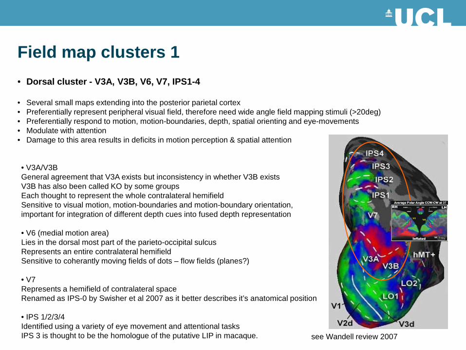
Field map clusters 1• Dorsal cluster - V3A, V3B, V6, V7, IPS1-4

• Several small maps extending into the posterior parietal cortex• Preferentially represent peripheral visual field, therefore need wide angle field mapping stimuli (>20deg)• Preferentially respond to motion, motion-boundaries, depth, spatial orienting and eye-movements• Modulate with attention• Damage to this area results in deficits in motion perception & spatial attention

• V3A/V3BGeneral agreement that V3A exists but inconsistency in whether V3B existsV3B has also been called KO by some groupsEach thought to represent the whole contralateral hemifieldSensitive to visual motion, motion-boundaries and motion-boundary orientation, important for integration of different depth cues into fused depth representation

• V6 (medial motion area)Lies in the dorsal most part of the parieto-occipital sulcusRepresents an entire contralateral hemifieldSensitive to coherantly moving fields of dots – flow fields (planes?)

• V7 Represents a hemifield of contralateral spaceRenamed as IPS-0 by Swisher et al 2007 as it better describes it’s anatomical position

• IPS 1/2/3/4 Identified using a variety of eye movement and attentional tasksIPS 3 is thought to be the homologue of the putative LIP in macaque. see Wandell review 2007

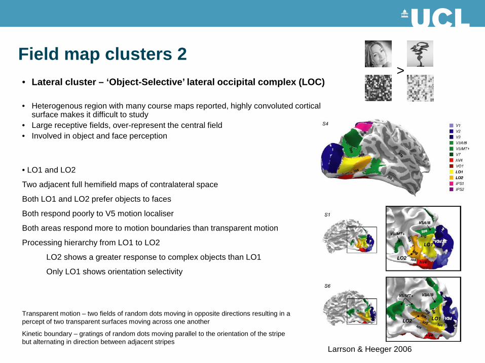
Field map clusters 2

• LO1 and LO2

Two adjacent full hemifield maps of contralateral space

Both LO1 and LO2 prefer objects to faces

Both respond poorly to V5 motion localiser

Both areas respond more to motion boundaries than transparent motion

Processing hierarchy from LO1 to LO2

LO2 shows a greater response to complex objects than LO1

Only LO1 shows orientation selectivity

Transparent motion – two fields of random dots moving in opposite directions resulting in a percept of two transparent surfaces moving across one another

Kinetic boundary – gratings of random dots moving parallel to the orientation of the stripe but alternating in direction between adjacent stripes

>

Larrson & Heeger 2006

• Lateral cluster – ‘Object-Selective’ lateral occipital complex (LOC)

• Heterogenous region with many course maps reported, highly convoluted cortical surface makes it difficult to study

• Large receptive fields, over-represent the central field• Involved in object and face perception

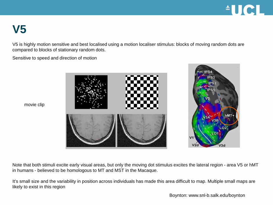
V5V5 is highly motion sensitive and best localised using a motion localiser stimulus: blocks of moving random dots are compared to blocks of stationary random dots.

Sensitive to speed and direction of motion

Note that both stimuli excite early visual areas, but only the moving dot stimulus excites the lateral region - area V5 or hMT in humans - believed to be homologous to MT and MST in the Macaque.

It’s small size and the variability in position across individuals has made this area difficult to map. Multiple small maps are likely to exist in this region

Boynton: www.snl-b.salk.edu/boynton

movie clip

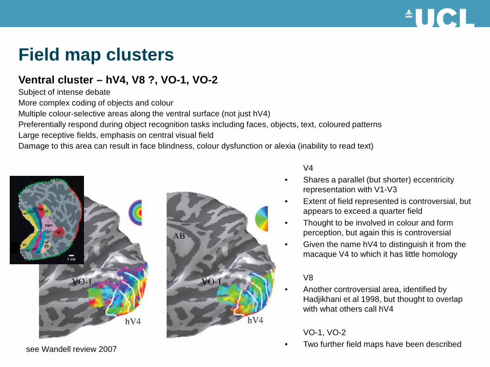
Field map clustersVentral cluster – hV4, V8 ?, VO-1, VO-2Subject of intense debateMore complex coding of objects and colourMultiple colour-selective areas along the ventral surface (not just hV4) Preferentially respond during object recognition tasks including faces, objects, text, coloured patternsLarge receptive fields, emphasis on central visual fieldDamage to this area can result in face blindness, colour dysfunction or alexia (inability to read text)

V4• Shares a parallel (but shorter) eccentricity

representation with V1-V3• Extent of field represented is controversial, but

appears to exceed a quarter field• Thought to be involved in colour and form

perception, but again this is controversial• Given the name hV4 to distinguish it from the

macaque V4 to which it has little homology

V8• Another controversial area, identified by

Hadjikhani et al 1998, but thought to overlap with what others call hV4

VO-1, VO-2• Two further field maps have been describedsee Wandell review 2007

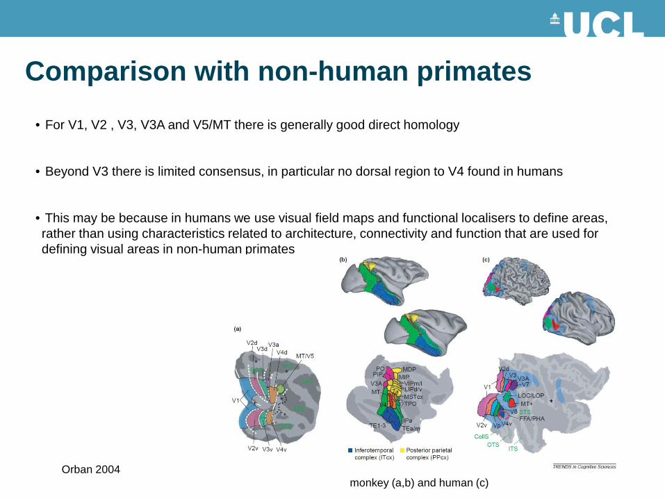
Comparison with non-human primates• For V1, V2 , V3, V3A and V5/MT there is generally good direct homology

• Beyond V3 there is limited consensus, in particular no dorsal region to V4 found in humans

• This may be because in humans we use visual field maps and functional localisers to define areas, rather than using characteristics related to architecture, connectivity and function that are used for defining visual areas in non-human primates

monkey (a,b) and human (c)Orban 2004

Beyond Retinotopic Cortex

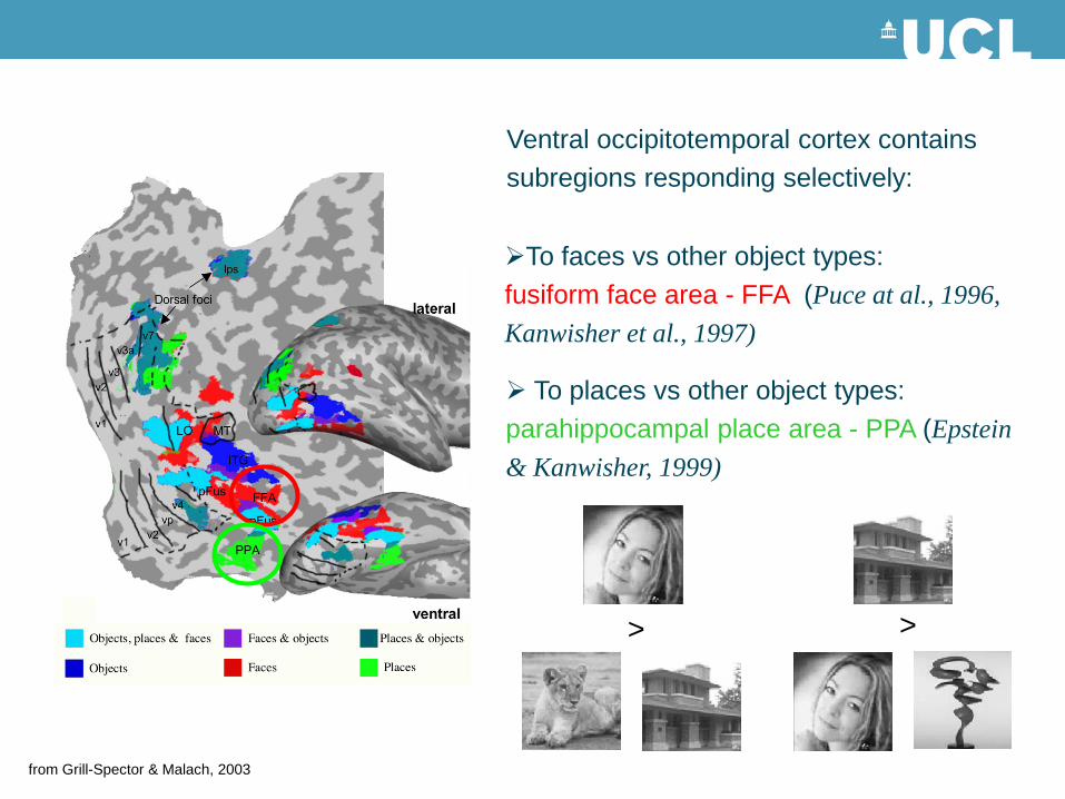
Ventral occipitotemporal cortex contains subregions responding selectively:

>

from Grill-Spector & Malach, 2003

To faces vs other object types: fusiform face area - FFA (Puce at al., 1996, Kanwisher et al., 1997)

To places vs other object types: parahippocampal place area - PPA (Epstein & Kanwisher, 1999)

>

Effect of attention on fMRI activity

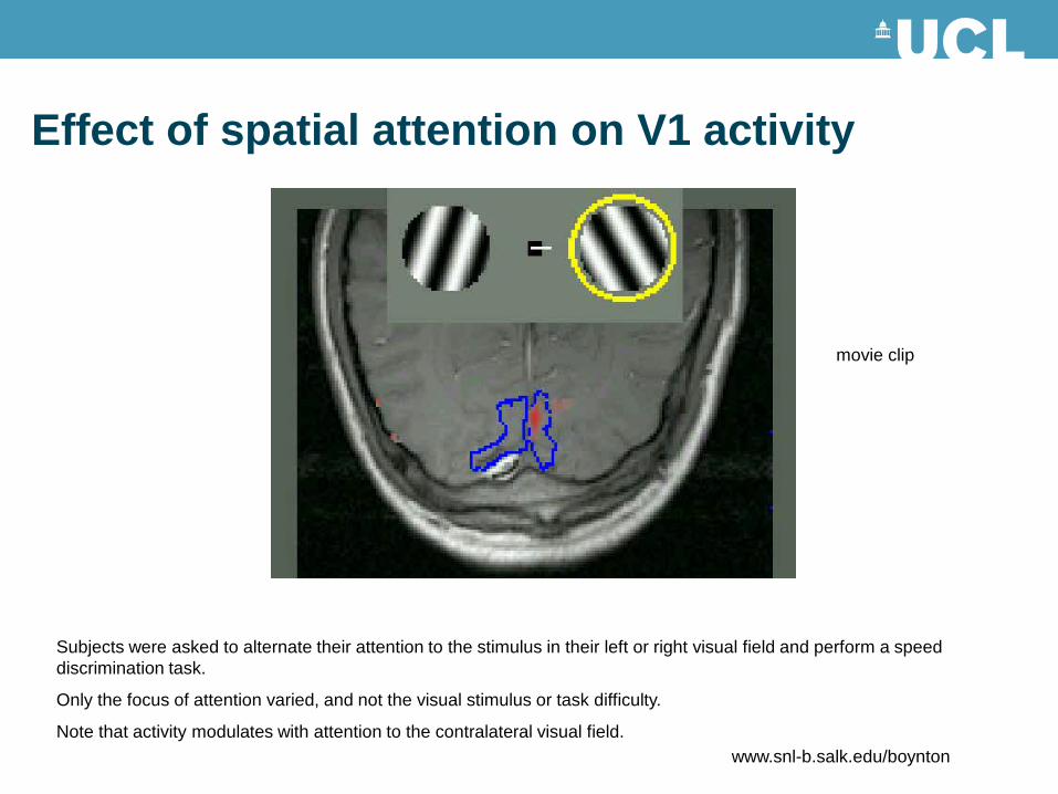
Effect of spatial attention on V1 activity

Subjects were asked to alternate their attention to the stimulus in their left or right visual field and perform a speed discrimination task.

Only the focus of attention varied, and not the visual stimulus or task difficulty.

Note that activity modulates with attention to the contralateral visual field. www.snl-b.salk.edu/boynton

movie clip

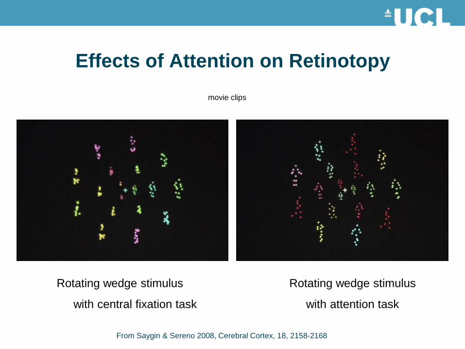
Effects of Attention on Retinotopy

Rotating wedge stimulus Rotating wedge stimulus

with central fixation task with attention task

From Saygin & Sereno 2008, Cerebral Cortex, 18, 2158-2168

movie clips

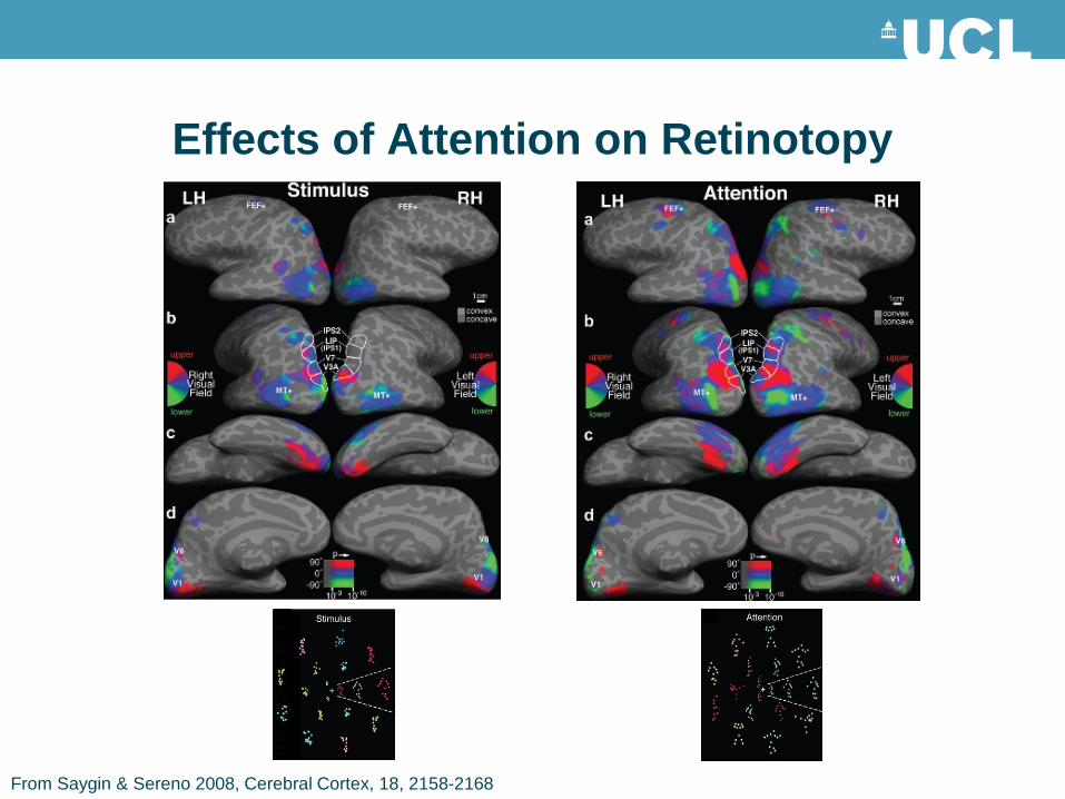
Effects of Attention on Retinotopy

From Saygin & Sereno 2008, Cerebral Cortex, 18, 2158-2168

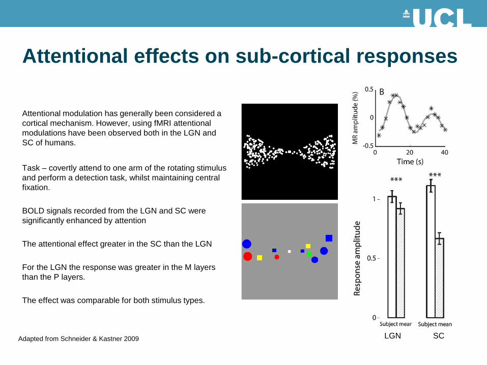
Attentional effects on sub-cortical responses

Attentional modulation has generally been considered a cortical mechanism. However, using fMRI attentional modulations have been observed both in the LGN and SC of humans.

Task – covertly attend to one arm of the rotating stimulus and perform a detection task, whilst maintaining central fixation.

BOLD signals recorded from the LGN and SC were significantly enhanced by attention

The attentional effect greater in the SC than the LGN

For the LGN the response was greater in the M layers than the P layers.

The effect was comparable for both stimulus types.

LGN SCAdapted from Schneider & Kastner 2009

Summary

• fMRI - new technique, non-invasive, good spatial resolution• BOLD signal – concentration of oxygenated blood varies with neural activity• Activation maps represent how well the BOLD signal matches the time course of

the stimulus• The spatial representation of an image is preserved in retinotopic maps

throughout early visual cortex, as well as sub-cortical areas• V1-V8 have been identified using visual field mapping techniques• Field map clusters:

– Dorsal cluster – motion, motion boundaries, depth, spatial attention– Lateral cluster – object processing and motion– Ventral cluster – colour-selective, objects, faces

• Attention can enhance BOLD responses in cortical as well as sub-cortical regions

ReferencesN. Logothetis. What we can do and what we cannot do with fMRI. Nature, 2008, 453, 869-878

M. Raichle & M. Mintun, Brain Work and Brain Imaging, Annual Review of Neuroscience 2006, 29:449-76

P. M. Matthews & P. Jezzard, Functional Magnetic Resonance Imaging, Neurol Neurosurg Psychiatry 2004 75: 6-12

D. O’Connor et al. Attention modulates responses in the human lateral geniculate nucleus. Nature, 2002, 5(11), 1203-1209

K.A. Schneider et al. Retinotopic organisation and Functional Subdivisions of the Human lateral geniculate nucleus: A High-Resolution Functional Magnetic Resonance Imaging Study. J Neuroscience,2004, 24(41), 8975-8985.

R. Sylvester et al. J Neurophysiol, 2007, 97: 1495–1502

K.A. Schneider, et al. Visual responses of the Human superior colliculus: A High-resolution functional magnetic resonance imaging study. J Neurophysiol, 2005, 94:2491-2503

R. B. H. Tootell, et al. Functional analysis of primary visual cortex (V1) in humans. PNAS, 1998, 95, 811–817.

S. Pitzalis et al. Human V6: The Medial Motion Area. Cerebral Cortex, 2010;20:411—424.

E. Yacoub, et al. High-field fMRI unveils orientation columns in humans. PNAS, 2008, 105, 10607–10612.

K. Cheng, et al, Neuron, Vol. 32, 359–374, October 25, 2001

K. D. Singh, et al. Spatiotemporal Frequency and Direction Sensitivities of Human Visual Areas Measured Using fMRI. NeuroImage, 2000, 12, 550–564.

B. Wandell et al. Visual Field Maps in Human Cortex, Neuron, 2007, 56, 366-383

Dougherty et al. Visual Field Representations and Locations of Visual Areas V1/2/3 in Human Cortex, J Vision, 2003, 3, 586-598

Swisher et al. Visual Topography of Human Intraparietal Sulcus, 2007, J Neuroscience, 27(20), 5326-5337

Pitzalis et al. Wide-Field Retinopathy Defines Human Cortical Visual Area V6, JoN, 2006, 26(30), 7962-7973

A. Saygin and M.I. Sereno. Retinotopy and Attention in Human Occipital, Temporal, Parietal and Frontal Cortex, Cerebral Cortex, 2008, 18, 2158-2168

M.I. Sereno and R. Tootell From Monkeys to Humans:what do we now know about brain homologies? Current Opinion in Neurobiology, 2005, 15, 135-144

M.I. Sereno et al, Borders of Multiple Visual Areas in Humans Revealed by Functional Magnetic Resonance Imaging. Science, 1995, 268, 889-893

B. Wandell and Smirnakis. Plasticity and Stability of Visual Field Maps in Adult Primary Visual Cortex. Nature Reviews Neuroscience, 2009, 1-12.

G. A. Orban et al. Comparative mapping of higher visual areas in monkeys and humans. Trends in Cognitive Sciences, 8(7), 315-324

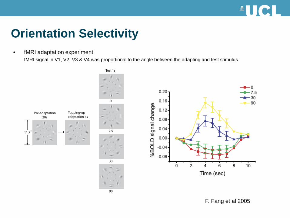
Orientation Selectivity• fMRI adaptation experiment

fMRI signal in V1, V2, V3 & V4 was proportional to the angle between the adapting and test stimulus

F. Fang et al 2005

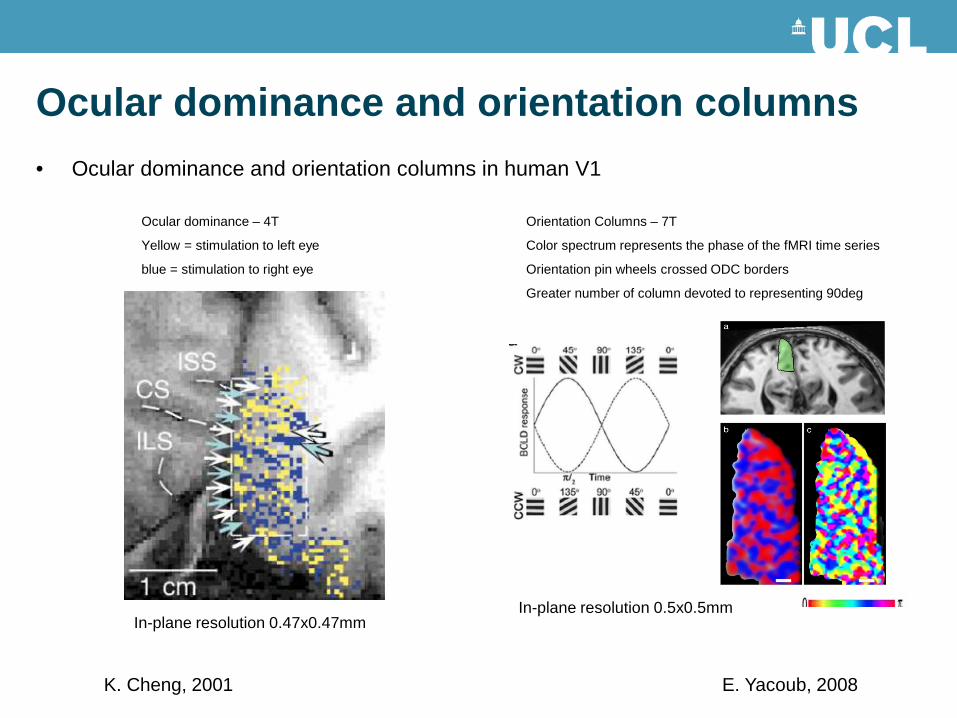
• Ocular dominance and orientation columns in human V1

Ocular dominance and orientation columns

Ocular dominance – 4T

Yellow = stimulation to left eye

blue = stimulation to right eye

K. Cheng, 2001

In-plane resolution 0.47x0.47mm

Orientation Columns – 7T

Color spectrum represents the phase of the fMRI time series

Orientation pin wheels crossed ODC borders

Greater number of column devoted to representing 90deg

E. Yacoub, 2008

In-plane resolution 0.5x0.5mm