fm as a controller - nasa

FM as a Controller

[email protected]

NASA Ames Research Center

mailto:[email protected]

Introduction

• Acknowledgements

• Fault Management (FM) as Controller

• Feedback Control Timeline

• AI Methods–Timeline

• Fault Management Timeline

• Assertion

• Modern Control Theory FM DRDs

• Conclusions

• References

Acknowledgements

• FM Conference

– Lorraine Fesq, John Day

• NASA Ames Line Management

– Dr. Ann Patterson-Hine, Dr. Eric Barszcz

• NASA Marshall SLS FM

– Stacy Cook, Jon Patterson, Dr. Stephen Johnson

• NASA ARC/JSC HA/AMO Autonomy/FM

– Dr. Mark Schwabacher, Dr. Jeremy Frank

Introduction






• Assertion


• Conclusions

• References

Fault Management (FM) as Controller

Spacecraft

Nominal Control

FDIR*

observations (y) commands (u)

state (xFM)

• Two loops – one nominal, one FDIR (FM). • View FM as a form of feedback control which

complements nominal control. • Leverage methodology of modern control theory.

goals/setpoints (rnom)

goals/setpoints (rFM)

Feedback Control - Definitions • Cybernetics: “The science of communication and

control in the animal and in the machine.” [Weiner 48]

• “Feedback control is the basic mechanism by which systems, whether mechanical, electrical, or biological, maintain their equilibrium or homeostasis. “[Lewis 1992]

• “Feedback control may be defined as the use of difference signals, determined by comparing the actual values of system variables to their desired values, as a means of controlling a system. Since the system output is used to regulate its input, such a device is said to be a closed-loop control system.” “[Lewis 1992]

Benefits

• Provides a common language for FM practitioners to communicate with Nominal Control practitioners

• Provides a framework to define FM Requirements and Data Requirement Definitions

• Provides a framework to define formal estimates of FM domain complexity to support model development and accreditation costing. - TBD

• Provides a framework to help determine FM FP/FN requirements through controller properties of stability, observability and stability - TBD

Introduction






• Assertion


• Conclusions

• References

Feedback Control Timeline • 300 BC – 1200 AD

– 3rd Century BC Ktesibios – Water Clock

• 1600 AD – 1875 AD Industrial Revolution – control of machines – 1620 Cornelius Drebbel – Temperature Regulator – 1780 James Watt - Governor – Pressure Regulator – Mathematics (Least Squares, DiffEq, Linear Algebra, Optimality)

• 1910 AD – 1945 AD – Frequency Domain Methods - Classic Control Theory – 1922 Minorsky Proportional-integral-derivative (PID) controller. – 1936 George Philbrick – Analog Computer for Process Control – 1948 N Wiener – “Cybernetics: or Control and Communication in the

Animal and Machine”

• 1957 AD – present – Time Domain Methods – Modern Control Theory – 1957 Sputnik – [Draper 1960] inertial navigation system (Polaris, and later Apollo AGC) – [Kalman 1960] “A New Approach to Linear Filtering and Prediction

Problems” – [Åström and Wittenmark 1971] “On Self-Tuning Regulators”

Abstracted from [Lewis 92] + additions

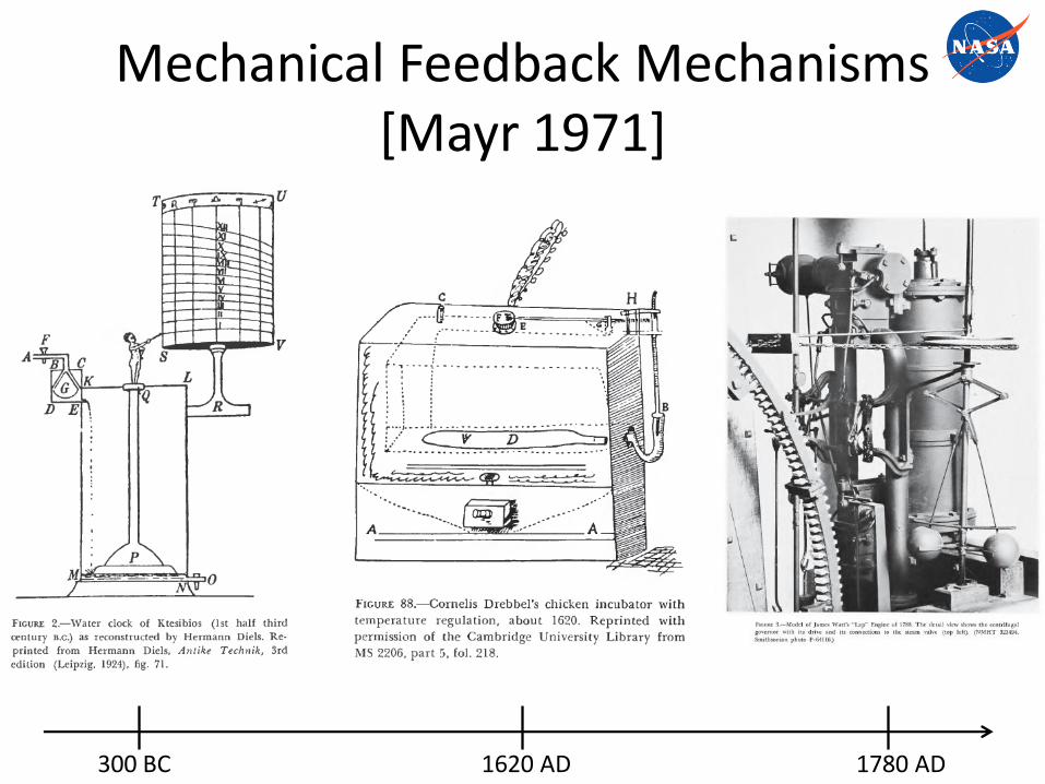
Mechanical Feedback Mechanisms [Mayr 1971]

300 BC 1620 AD 1780 AD

Period of Classical Control

PID Control Defined

1922 AD 1936 AD 1948 AD

Cybernetics: “The science of communication and control in the animal and in the machine.”

Frequency Domain Approaches

Period of Modern Control I

1957 1960 1960s

[Draper 1960] inertial navigation system (Polaris, and later Apollo AGC)

Sputnik

Time Domain Approaches

Period of Modern Control - II [Kalman 1960] “A New Approach to Linear Filtering and Prediction Problems”

Kalman’s Advances:

1. time-domain approach

2. linear algebra and matrices

3. the concept of the internal system state

4. the notion of optimality in control theory

Period of Modern Control - II [Åström and Wittenmark 1971] “On Self-Tuning Regulators”

“ An adaptive controller can be thought of as having two loops. One loop is normal feedback with the process[plant] and the controller. The other loop is the parameter adjustment loop. ” [Åström and Wittenmark 1995 ]

Parameter Adjustment

Controller Plant

Figure 1.1 Block diagram of an adaptive system. [Åström and Wittenmark 1995 ]

Setpoint

Control parameters

Control signal

Output

Introduction






• Assertion


• Conclusions

• References

AI Methods–Timeline

• 1957 - present – [Newell, Simon, Shaw 1958] ““Report of a

General Problem-Solving Program” – 1972 [Nilsson 1984] “Shakey The Robot”

– [Brooks, 1986] Brooks, R.A., "A robust layered control system for a mobile robot

– [Williams, Nayak 1996] – NASA Deep Space 1 – Remote Agent Experiment

– [Dvorak et al 2000] Mission Data Systems

AI Methods I

1957 1972

[Newell, Simon, Shaw 1958] ““Report of a General Problem-Solving Program”

[Nilsson 1984] “Shakey The Robot”

AI Methods II • [Brooks, 1986] Brooks, R.A., "A robust layered control system for a mobile

robot” • Moved away from traditional AI approaches to layers of feedback loops.

Old Approach

New Approach

AI Methods III • [Williams, Nayak 1996] – NASA Deep Space 1 Remote Agent

Experiment (RAX) • MI – Mode Identification, MR – Mode Recovery • MI, MR – Model-Based (schematic network, each with FSM)

<Picture of DS1>

AI Methods IV

• [Dvorak et al 2000] Mission Data Systems

• Model-Based

Introduction






• Assertion


• Conclusions

• References

Fault Management Timeline

• 1990 – Present – [Johnson 1994] – “VHM Generic Architecture”

– [Leveson 1995] – “Safeware – System Safety and Computers”

– [Robinson 2003] – “Applying Model-Based Reasoning to the FDIR of the Command & Data Handling Subsystem of the International Space Station”

– [Dulac et al. 2007] “Demonstration of a New Dynamic Approach to Risk Analysis for NASA’s Constellation Program” Leveson (PI)

– [NPR-8705.2B] NASA Human-Rating Requirements for Space Systems

Fault Management - I

• [Johnson 1994] “VHM Generic Architecture” Dr. Stephen Johnson – personal communication

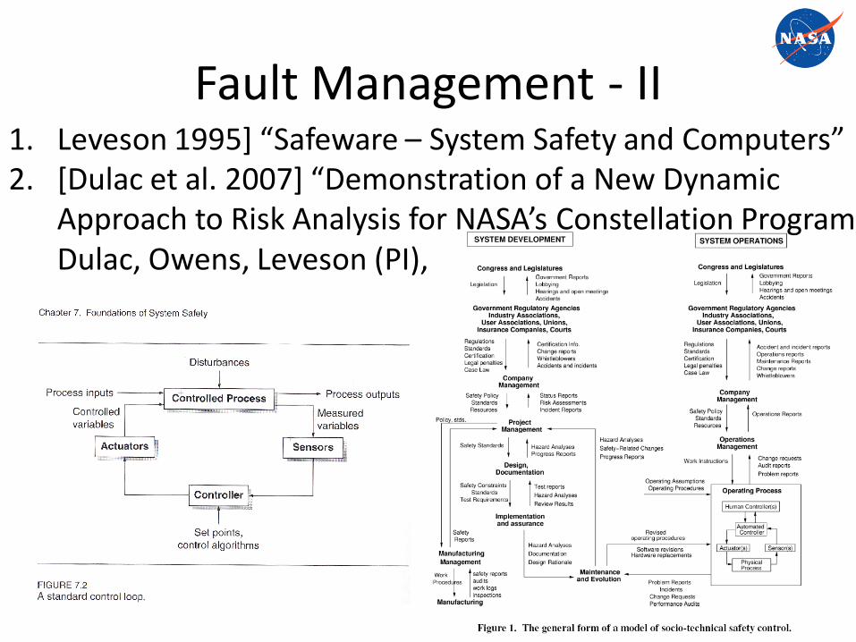
Fault Management - II

1. Leveson 1995] “Safeware – System Safety and Computers” 2. [Dulac et al. 2007] “Demonstration of a New Dynamic

Approach to Risk Analysis for NASA’s Constellation Program” Dulac, Owens, Leveson (PI),

Fault Management III • [Robinson et al. 2003] “Applying Model-Based Reasoning

to the FDIR of the Command & Data Handling Subsystem of the International Space Station”

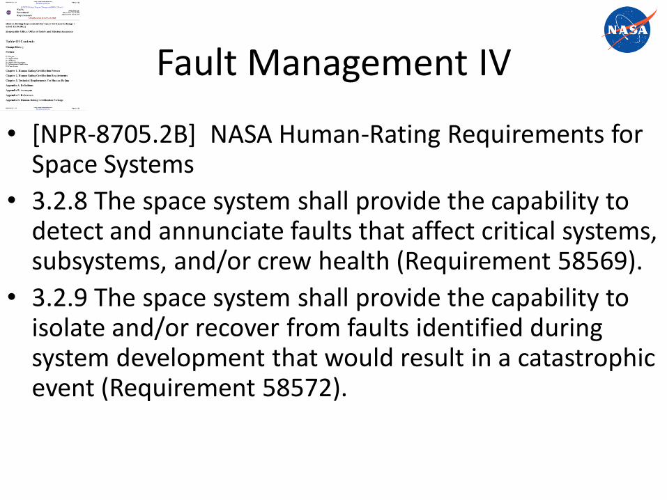
Fault Management IV

• [NPR-8705.2B] NASA Human-Rating Requirements for Space Systems

• 3.2.8 The space system shall provide the capability to detect and annunciate faults that affect critical systems, subsystems, and/or crew health (Requirement 58569).

• 3.2.9 The space system shall provide the capability to isolate and/or recover from faults identified during system development that would result in a catastrophic event (Requirement 58572).

Introduction






• Assertion


• Conclusions

• References

Assertion Fault Management can be formally modeled as a feedback control process using concepts from modern control theory.

Evidence • [Dean, Wellman 1991] “Planning & Control” • First formal attempt to bridge the gap between

AI symbolic methods and traditional control. • AI Methods Identify Three Types of Goals:

– Achievement – Maintenance – Prevention.

• What do they both have in common with FM? – The concept of state – however AI methods

tend to blur state vs. observations – The ability to measure a difference between

the objective and the current state. – Use of the difference to drive the next

action. – Goals of Maintenance

Formal Modeling of Feedback Loops

• [Robinson 1997a] “Feedback to Basics” (AAAI) Fall Symposium Model-Directed Autonomous Systems

• [Robinson 1997b] “Autonomous design and execution of process controllers for untended scientific instruments”, AGENTS '97 Proceedings of the first international conference on Autonomous agents, ACM

• [Robinson 2001] “Automatic Overset Grid Generation with Heuristic Feedback Control” NASA/TM-2001-210931 November 2001.

• [Robinson 2003] “Applying Model-Based Reasoning to the FDIR of the Command & Data Handling Subsystem of the International Space Station”, Robinson et. al. -SAIRAS 2003

• [Robinson 2005] “A Three Level Autonomous Software System for Increased Science Return” Robinson et. Al., American Geophysical Union, Fall Meeting 2005

Modern Control Theory

• Kalman’s Key Points

– time-domain approach

– linear algebra and matrices

– internal system state

– the notion of optimality

MCT Definition [Kalman 60]

[Brogan 1982]

State equation: x’ = Ax + Bu Observation equation: y = Cx Gain Equation: u(t) = -Kx

Introduction






• Assertion


• Conclusions

• References

Modern Control Theory FM DRDs

• DRD 1 – Define variables and values

• DRD 2 – Define matrices which relate variables

• DRD 3 – Define control law equations from matrices and variables –TBD

• DRD 4 – Define properties of controller - TBD

Data Requirements Definition 1

• Define vector variables r,y,x,u,e for the domain(s)

Controller Parameter

Variable Name

Vector Size

Possible Values (each element)

setpoints r l x 1 reals, integers, discretes

observations y m x 1 reals, integers, discretes

state variables

x n x 1 reals, integers, discretes

loads u r x 1 reals, integers, discretes

error e l x 1 reals, integers, discretes

Variable Mapping: Spacecraft Products -> Control Theory

total spacecraft state space (x)

nominal spacecraft state space (x)

flight rules (x)

flight procedures/software (u)

CW event (off-nominal state) (e)

nominal event (sensors, state)) (y,x)

spacecraft schematics (x)

r – setpoint vector (l x 1)

ppm

ppm

atm

levelNOcabin

levelCOcabin

pressurecabin

tempcabin

r

r

r

r

r

l

nom

250

25

1

°C20

_2

_

_2

_

_

_

3

2

1

11

3

2

1

_

_

_

_

Mode

working

working

working

state

stateTVC

statecooler

statefuelpump

r

r

r

r

SW

r

l

FM

• Each element of the r vector defines a setpoint for the system

• Different r vector for nominal control vs FM control.

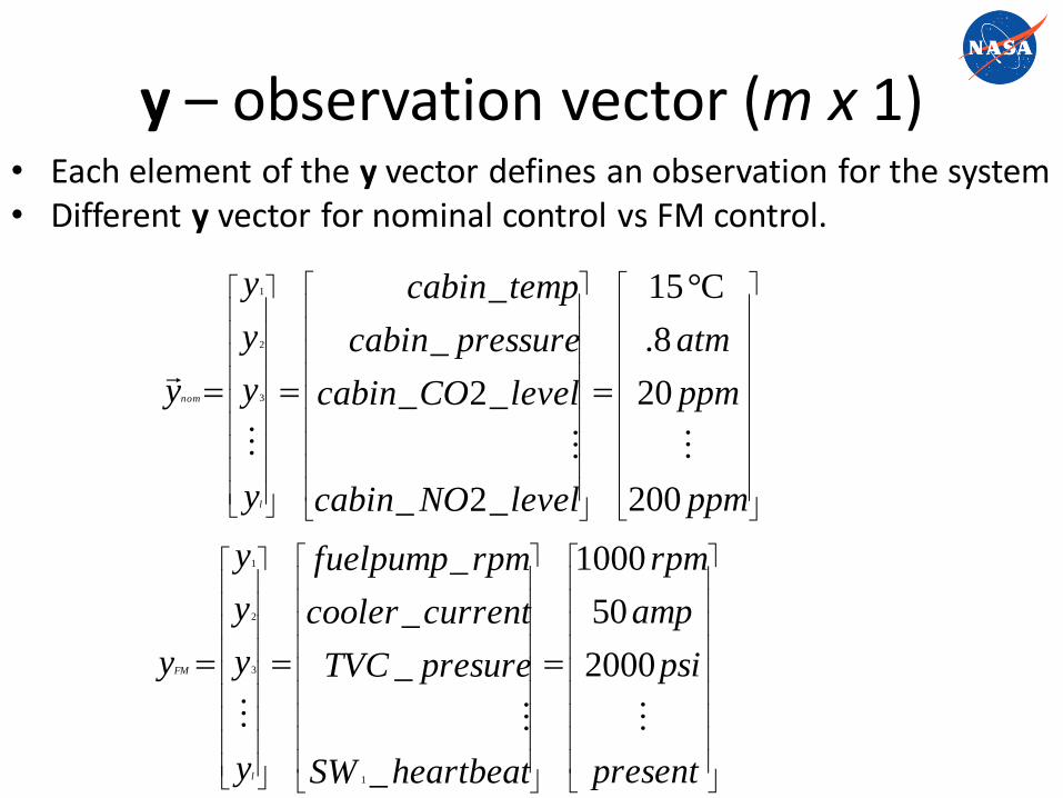
y – observation vector (m x 1)

ppm

ppm

atm

levelNOcabin

levelCOcabin

pressurecabin

tempcabin

y

y

y

y

y

l

nom

200

20

8.

°C15

_2_

_2_

_

_

3

2

1

present

psi

amp

rpm

heartbeatSW

presureTVC

currentcooler

rpmfuelpump

y

y

y

y

y

l

FM

2000

50

1000

_

_

_

_

1

3

2

1

• Each element of the y vector defines an observation for the system • Different y vector for nominal control vs FM control.

x – state vector (n x 1) • Each element of x defines a state variables for the system

• Different x vector for nominal control vs FM control.

bydS

working

failed

working

stateSW

stateTVC

statecooler

statepump

x

x

x

x

x

n

FM

tan_

_

_

_

1

3

2

1

liters

liters

C

liters

volumehydrazine

volumehydraulic

cecapacithermal

volumeO

x

x

x

x

x

n

nom

2

5

50

20

_

_

tan_

_2

3

2

1

u – load vector (r x 1)

scrubberoffonturn

tvcretractextend

pumpoffonturn

valveoffonturn

COscrub

nozzlegimbal

cabininaircirculate

directionzinthrustapply

u

u

u

u

u

r

nom

/

/

/

/

2_

_

___

____

3

2

1

offonturn

offonturn

offonturn

offonturn

componentSW

componentHW

cooler

pumpfuel

u

u

u

u

u

j

i

r

FM

/

/

/

/_

3

2

1

• Each element of u defines a loads/commands for the system

• Different u vector for nominal control vs FM control.

e – error vector • Two types of error, observation vs. state error. • What does symbolic difference mean? (points to transition between

two states of an FSM)

50

5

2.

5

250

25

1

°C20

200

20

8.

°C15

_2_

_2_

_

_

3

2

1

3

2

1

3

2

1

ppm

ppm

atm

ppm

ppm

atm

r

r

r

r

y

y

y

y

levelNOcabin

levelCOcabin

pressurecabin

tempcabin

e

e

e

e

e

mmm

nom

11 tantan_1

_

_

_

3

2

1

ModedbyS

workingfailed

Mode

working

working

working

bydS

working

failed

working

stateSW

stateTVC

statecooler

statepump

e

e

e

e

e

n

FM

Data Requirements Definition 2 • Matrices which relate y,x,u • Definitions for the matrices forces

modelers to be systematic. • y=Cx

– What is the state x wrt to the sensors y?

• x’=Ax+Bu – How does the state x affect the change

of the state x?

• x’=Ax+Bu: – How does next loads/actions u affect

the change of state x’.

• u=-Kx: – What should the next action u be given

the current state x?

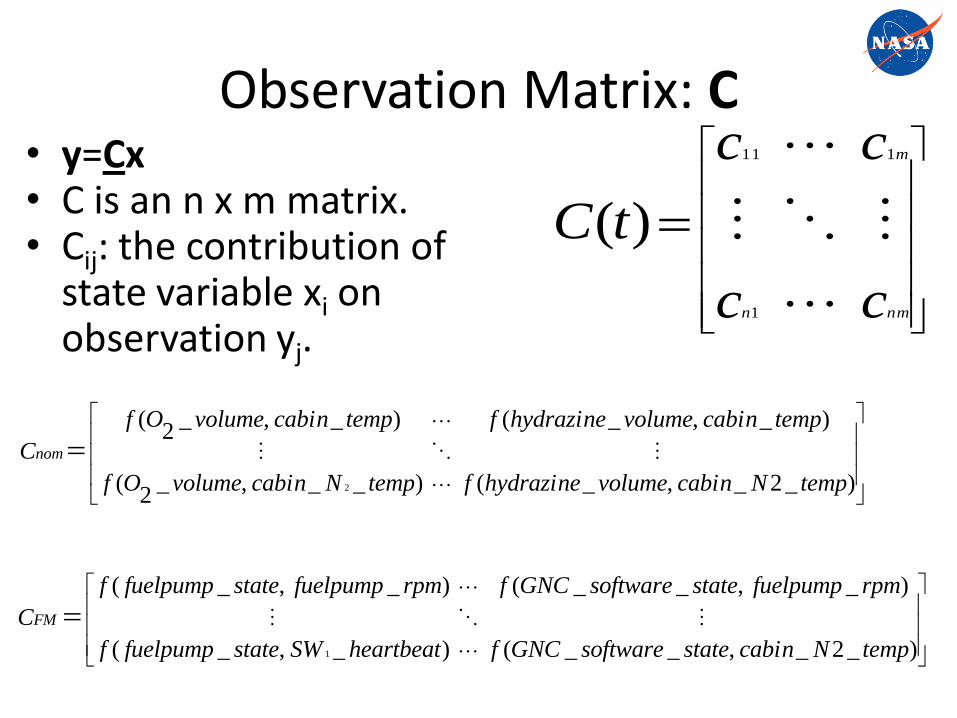
Observation Matrix: C

• y=Cx • C is an n x m matrix. • Cij: the contribution of

state variable xi on observation yj.

nmn

m

cc

cc

tC

1

111

)(

)_2_,__()_,_(

)_,__()_,_(

1 tempNcabinstatesoftwareGNCfheartbeatSWstatefuelpumpf

rpmfuelpumpstatesoftwareGNCfrpmfuelpumpstatefuelpumpf

CFM

)_2_,_()__,_

2(

)_,_()_,_2

(

2 tempNcabinvolumehydrazineftempNcabinvolumeOf

tempcabinvolumehydrazineftempcabinvolumeOf

Cnom

x=C†y

• Note: pseudo inverse (or true inverse) of the observation equation is diagnosis.

• For diagnosis, the inverse is not unique – due to the fact that there are significantly less sensors than state variables.

• A selling point for FM methods, as many traditional control methods will fail due to non-unique inverse.

state vector

State vector element failed

State vector element working

Non-unique Inverse

Livingstone Example: Support for non-unique inverse [Robinson 2003]

State Transition Matrix: A

• x’=Ax+Bu • A is an n x n matrix. • Aij: the contribution of state variable xi on the change

of state variable xj. • State Transition

• Numeric systems: Derivative • Symbolic systems: Finite State Transition

nnn

n

aa

aa

A t

1

111

)(

Nominal and FM A Matrix

)_,_()_,_2(

)_2,_()_2,_2(

volumehydrazinevolumehydrazinefvolumehydrazinevolumeOf

volumeOvolumehydrazinefvolumeOvolumeOf

nomA

)_,_()_,_(

)_,_()_,_(

111

1

stateSWstateSWfstateSWstatepumpf

statepumpstateSWfstatepumpstatepumpf

FMA

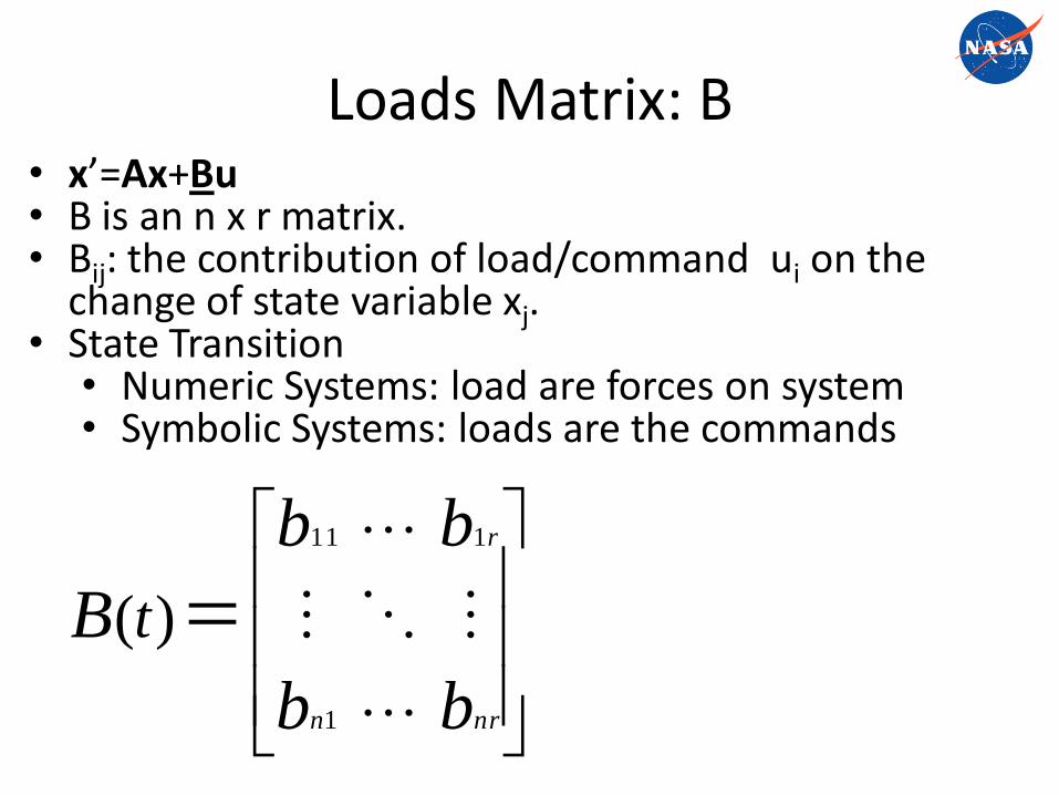
Loads Matrix: B

• x’=Ax+Bu • B is an n x r matrix. • Bij: the contribution of load/command ui on the

change of state variable xj. • State Transition

• Numeric Systems: load are forces on system • Symbolic Systems: loads are the commands

nrn

r

bb

bb

B t

1

111

)(

Nominal and FM B Matrix

)_/,_()_/,_2(

)_/,_()_/,_2(

scrubberoffturnonvolumehydrazinefscrubberoffturnonvolumeOf

valveoffturnonvolumehydrazinefvalveoffturnonvolumeOf

nomB

)_/,_()_/,_(

)_/,_()_/,_(

111

1

SWoffturnonstateSWfSWoffturnonstatepumpf

fuelpumpoffturnonstateSWffuelpumpoffturnonstatepumpf

FMB

Gain Matrix: K

• u=-Kx • K is an n x r matrix. • Kij: the contribution of the state variable xi on the

next load uj.

nrn

r

kk

kk

tK

1

111

)(

Nominal and FM K Matrix

)_/,_()_/,_2(

)_/,_()_/,_2(

scrubberoffturnonvolumehydrazinefscrubberoffturnonvolumeOf

valveoffturnonvolumehydrazinefvalveoffturnonvolumeOf

nomK

)1_/,_1()1_/,_(

)_/,_1()_/,_(

SWoffturnonstateSWfSWoffturnonstatepumpf

fuelpumpoffturnonstateSWffuelpumpoffturnonstatepumpf

FMK

DRD 3 Control Law Equations - TBD

nnmn

m

m x

x

cc

cc

y

y

1

1

1111

rnrn

r

nnnn

n

n u

u

bb

bb

x

x

aa

aa

x

x

1

1

1111

1

1111

nnrn

r

r x

x

kk

kk

u

u

1

1

1111

Gain Equation: u(t) = -Kx

State equation: x’ = Ax + Bu

Observation equation: y = Cx

DRD 4 Controller Properties - TBD

• Modern Control Theory provides methods to prove properties for controllability, observability and stability.

• How do these methods translate to symbolic reasoning domains?

Comparison of Modeling Primitives Property Nominal Control FM Control

Function Definition Domain, Range in Reals Finite State Machines/Table Lookup

Derivative of Function Function Derivative or Difference

Finite State Transition

Integration of Function Summation of Derivative State Transition Path from Initial to Final State.

Modeling Primitive Equation Generalized Constraint (components)

System of Equations System of Equations, Linear Algebra operations

Hierarchical Network of HW/SW components, modified Linear Algebra operations (symbolic inner-product methods).

Matrix Inverse Capabilities (x=C-†y)

Fails – due to under /over constrained system

No failure! – part of FM architecture to handle.

Linearity Assumption: (scalability, super-position properties)

Foundation of MCT Reflected into fault signatures/ responses which are independent. (i.e. multiple fault signatures are additive)

Solving for K (control policy).

Gradient descent search for minima or maxima

Search through parallel FSMs, enforcing temporal constraints

Introduction






• Assertion


• Conclusions

• References

Conclusions

• Use of generalized linear algebra formalism: – provides a common language for FM practitioners to

communicate with Nominal Control practitioners

– Provides a methodology to systematically explore the complexity of the domain.

– Provides a methodology which supports scalability for extremely large systems ( e.g. 50K failure modes, 50K tests).

• However …. Matrix methods will break down and where they do innovations should be implemented to interface with generalized linear algebra methods.

Introduction






• Assertion


• Conclusions

• References

References I • [Weiner 1948] “Cybernetics: or Communication in the Animal and the Machine” – MIT Press • [Kalman 1960] "A New Approach to Linear Filtering and Prediction Problems,“ Kalman, R.E., ASME J. Basic Eng.,

vol. 82, pp.34-45, 1960. • [Newell,Shaw,Simon 1958] “Report of a General Problem-Solving Program” The RAND Corportation, Cargnegie

Institute of Technology • [Newell 1969] “Heuristic Programming: Ill-Structured Problems” • [Sorenson 1970] “Least-squares estimation: from Gauss to Kalman” Sorenson, H. IEEE Spectrum, vol. 7, pp. 63-

68, July 1970. • [Mayr 1970] “Origins of Feedback Control” Otto Mayr 1970 MIT Press • [Mayr 1971] “Feedback Mechanisms In the Historical Collections of the National Museum of History and

Technology” Smithsonian Institution Press 1971 • [Åström and Wittenmark 1972] “On Self-Tuning Regulators” 5th IFAC Conferernce • [Lewis 1992] “A Brief History of Feedback Control”, Chapter 1: Introduction to Modern Control Theory,

F.L.Lewis, Prentice Hall 1992, http://arri.uta.edu/acs/history.htm • [Johnson 1994] “VHM Generic Architecture” Dr. Stephen Johnson – personal communication • [Leveson 1995] “Safeware – System Safety and Computers” • [Åström and Wittenmark 1995] “Adaptive Control” 2nd Edition, Åström and Wittenmark 1995 Addison-Wesley

Publishing Company • [Willams, Nayak 1996] “A Model-based Approach to Reactive Self-Coniguring Systems” AAAI-96 • [Robinson 1997a] “Feedback to Basics” (AAAI) Fall Symposium Model-Directed Autonomous Systems • [Robinson 1997b] “Autonomous design and execution of process controllers for untended scientific

instruments”, AGENTS '97 Proceedings of the first international conference on Autonomous agents, ACM • [Dvorak et. al 2000] “Software Architecture Themes in JPL’s Mission Data System” Dvorak, Rasmussen, Reeves,

Sacks, IEEE Aerospace 2000 conference March 2000

http://arri.uta.edu/acs/history.htm

References II

• [Robinson 2001] “Automatic Overset Grid Generation with Heuristic Feedback Control” NASA/TM-2001-210931 November 2001.

• [Robinson et. al 2003] “Applying Model-Based Reasoning to the FDIR of the Command & Data Handling Subsystem of the International Space Station”, Robinson et. al. -SAIRAS 2003

• [Dulac et al. 2007] “Demonstration of a New Dynamic Approach to Risk Analysis for NASA’s Constellation Program” Dulac, Owens, Leveson (PI),

• [Brooks, 1986] Brooks, R.A., "A robust layered control system for a mobile robot", IEEE Journal of Robotics and Automation, Volume 2(1), 1986.

• [INM] “Sextant, Apollo Guidance and Navigation System” The Institute of Navigation – Navigation Museum” <cite http>

• [Nilsson 1984] Nilsson, Nils, “Shakey The Robot” SRI International Tech Report 1984

• [NPR-8705.2B] NASA Human-Rating Requirements for Space Systems

fm as a controller - nasa

Documents