16th Annual CFD Symposium 11th-12th August 2014, Bangalore 1

Flow past 6:1 prolate spheroid - A numerical study

A. Rajesh ∗ K. N. Vinay Kumar † M. B. Subrahmanya‡ D. S. Kulkarni‡ B.N.Rajani ‡∗ Project Assistant, CTFD Division, CSIR-NAL, Bangalore 560 017, India

†Student, Dept. of Mech. Engg, SSIT Tumkur 572 107, India‡Scientist, CTFD Division, CSIR-NAL, Bangalore 560 017, India

AbstractNumerical simulation of the three dimensional flow past 6 : 1 prolate spheroid at α = 20◦ and Re = 4.2× 106

using RANS approach has been carried out using the parallel version of the in-house structured grid multiblockflow solution code 3D-PURLES. The SST turbulence model is used to simulate the fully turbulent case and thismodel is suitably modified to handle transitional flows by fixing the onset of transition. The results thus obtainedare validated against the available measurement and/or computational data.

Keywords: Prolate spheroid, SST turbulence model, fixed transition, finite volume method, parallel computing.

1 IntroductionThree dimensional flow past prolate spheroids with different aspect ratios can be considered as simplified modelsof submarines, unmanned underwater vehicles, missiles, airships etc. The prolate spheroids are geometricallysimple but the flow characteristics are dominated by complex flow phenomenon like separation and transition. Thethree dimensional transitional flow with separation is one of the most challenging problems in fluid dynamics.Inspite of continuous research, the physics of three dimensional separation and the process of transition is not yetfully understood. The lack of proper understanding and non-availability of appropriate and accurate models forseparated turbulent and transitional flows forms a stumbling block for accurate flow predictions using the CFDtools. Several measurements and simulations for flow over prolate spheroids have been documented for surfacepressure and skin friction coefficient, profile of mean and turbulence quantities and also details of the separatedregion at various angle of attack [1, 4]. The paper presents the flow around 6 : 1 prolate spheroid at 20◦ angle ofattack for Re = 4.2× 106 for which experimental data [2, 12] and LES computation results [4] are available. Thepresent simulation has been carried out using the in-house flow solution code 3D-PURLES treating the flow to befully turbulent and also by fixing the onset of transition based on measurement data.

2 Finite Volume Method

2.1 Governing EquationsThe phase-averaged Navier Stokes equation for unsteady turbulent incompressible flow in non-orthogonal curvi-linear coordinates with cartesian velocities as dependent variables in a compact form are as follows:

Momentum transport for the Cartesian velocity component 〈Ui〉:

∂

∂t(ρ〈Ui〉) +

1J

∂

∂xj

[ρ〈Ui〉〈Uk〉βj

k + 〈P 〉βji −

µ

J

(∂〈Ui〉∂xm

Bjm +

∂〈Uk〉∂xm

βmi βj

k

)− ρ〈uiuj〉βj

k

]= SUi (1)

∗Corresponding author. Email: rajeshamech@gmail.com

2

where, 〈P 〉 and 〈Ui〉 are the phase-averaged pressure and velocity components along i direction respectively. µis the fluid viscosity, Bj

k and bjk are the metric coefficients due to transformation from cartesian to curvilinear

coordinates and J is the Jacobian of the transformation matrix. ui is the fluctuating velocity components and SUi

is any momentum source other than the pressure gradient These momentum equations are further supplemented bythe mass conservation or the so-called continuity equation.

Mass conservation (Continuity):

∂

∂xj

(ρ〈Uk〉βj

k

)= 0 (2)

The unknown turbulent stress term −ρ〈uiuj〉 is defined as follows based on the eddy viscosity hypothesis

−ρ〈uiuj〉 = µt

(∂〈Ui〉∂xj

+∂〈Uj〉∂xi

)− 1

3ρδij〈ukuk〉 (3)

where, δij is the Kronecker Delta and µt is the eddy viscosity which is an isotropic scalar quantity. The eddyviscosity is evaluated through turbulence modelling.

2.2 Numerical Solution of Finite Volume EquationThe present computation uses a general geometry, multiblock structured, pressure-based implicit finite volumealgorithm 3D-PURLES, developed at the CTFD Division, NAL Bangalore to solve the unsteady turbulent incom-pressible flow [8]. Central difference and other higher order upwind schemes have been used for spatial discreti-sation of the convective fluxes whereas the temporal derivatives are discretised using the second order accuratethree-level fully implicit scheme. An iterative decoupled approach similar to the SIMPLE algorithm [7], modifiedfor collocated variable arrangement [5] is adopted to avoid the checkerboard oscillations of the flow variables.The system of linear equations derived from the finite volume procedure is solved sequentially for the velocitycomponents, pressure correction and turbulence scalars using the strongly implicit procedure of Stone [10]. Thealgorithm is also successfully parallelized for cost effective computation on multiple processors using standardMPI routines. The present parallel computations have been carried out on the Altix-Ice cluster.

3 Results and DiscussionIn this study two different grids with O-O topology have been used (i) Coarse grid- 111×101×312 covered by 24blocks and (ii) Fine grid- 251× 161× 624 covered by 48 blocks. The non-dimensionalised near wall distance forboth the grids are maintained to be less than one. The schematic representation of the boundary condition and gridused are shown in Fig. 1. The unsteady computations have been carried out for Re = 4.2×106 based on the modellength (L) at α = 20◦ using the central difference scheme (CDS) coupled to deferred correction procedure [3] forspatial discretisation of convective flux and a second order accurate scheme for temporal discretisation with thenon-dimensionalised time step size of ∆t = 0.05. The simulations have been carried out assuming the flow to befully turbulent and also by fixing the transition onset location. The Shear Stress Transport (SST) model proposedby Menter [6] and the one equation model of Spalart-Allamaras (SA) [9] have been used for the fully turbulentcase. In the fixed transition case, the flow is tripped by fixing the transition onset location. The flow is treated aslaminar (µt = 0) upto the trip location and in the downstream µt is computed using the specified turbulence modelwhich is SST model in the present computation. Uniform flow is assumed at the farfield boundary with freestreamturbulence maintained at one percent and assuming the local eddy viscosity (µt) to be equal to the laminar viscosity(µ).

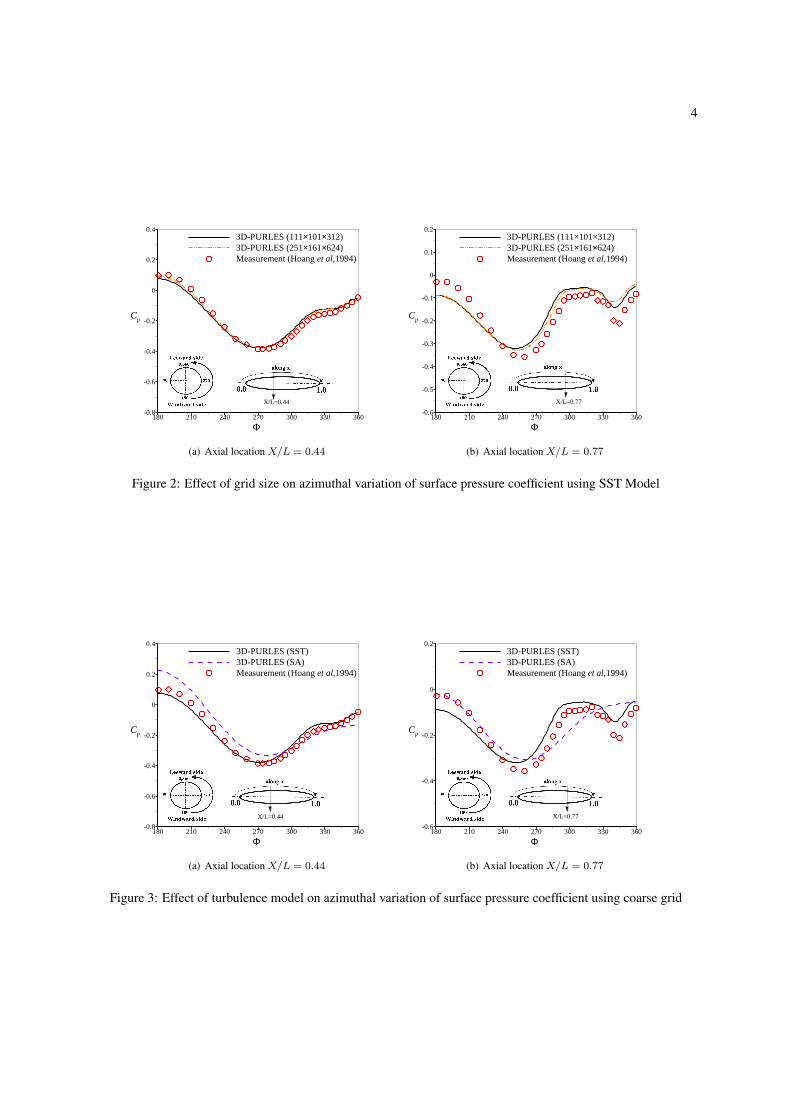
The effect of grid resolution on the azimuthal variation of the surface pressure coefficient (Cp) at two differentaxial locations (X/L = 0.44 and 0.77) obtained using SST turbulence model for α = 20◦ is shown in Fig. 2. Thefigure clearly indicates that refining the grid brings no significant change in the variation of the pressure coefficient

3

which is also reflected in the aerodynamic coefficient (Table. 1). The effect of turbulence model for the coarse gridresolution on the azimuthal variation of the surface pressure coefficient at the two axial locations for α = 20◦ isshown in Fig. 3. The figure clearly indicate that the SST turbulence model is in better agreement with the mea-surement data [2]. The deviation observed in the results obtained by SA model needs further investigation.

(a) Boundary conditions

X

Y

Z

(b) Near wall view of surface grid

Figure 1: Boundary condition and multiblock grid used for flow past prolate spheroid

Grid resolution Cl Cd Cm

Coarse - 111× 101× 312 0.0366 0.0176 -0.0206

Fine - 251× 161× 624 0.0371 0.0170 -0.0210

Table 1: Effect of grid size on aerodynamic coefficients

Simulations have also been carried out by fixing the transition onset location at X/L = 0.2 based on the mea-surement data [2, 11]. in the SST turbulence model. The surface streamlines and the contours of skin frictioncoefficient (Cf ) obtained for the coarse grid resolution (111 × 101 × 312) are shown in Fig. 4 and Fig. 5 respec-tively. It is evident from these figures that the skin friction contours as well as the surface streamlines obtained byfixing transition are significantly different from the fully turbulent case before the transition location (X/L = 0.2)and beyond which they are identical. It was also observed that the azimuthal variation of the surface pressure coef-ficient for the fully turbulent and fixed transition is different upto the trip location and elsewhere they are identical(plots not shown here). The flow pattern (Fig. 4) clearly indicates that the present simulation could capture theprimary and secondary separation as observed in the measurement data which confirms the adequacy of the gridresolution.

4

180 210 240 270 300 330 360-0.8

-0.6

-0.4

-0.2

0

0.2

0.43D-PURLES (111×101×312)3D-PURLES (251×161×624)Measurement (Hoanget al,1994)

Cp

Φ

X/L=0.44

(a) Axial location X/L = 0.44

180 210 240 270 300 330 360-0.6

-0.5

-0.4

-0.3

-0.2

-0.1

0

0.1

0.23D-PURLES (111×101×312)3D-PURLES (251×161×624)Measurement (Hoanget al,1994)

Cp

Φ

X/L=0.77

(b) Axial location X/L = 0.77

Figure 2: Effect of grid size on azimuthal variation of surface pressure coefficient using SST Model

180 210 240 270 300 330 360-0.8

-0.6

-0.4

-0.2

0

0.2

0.43D-PURLES (SST)3D-PURLES (SA)Measurement (Hoanget al,1994)

Cp

Φ

X/L=0.44

(a) Axial location X/L = 0.44

180 210 240 270 300 330 360-0.6

-0.4

-0.2

0

0.23D-PURLES (SST)3D-PURLES (SA)Measurement (Hoanget al,1994)

Cp

Φ

X/L=0.77

(b) Axial location X/L = 0.77

Figure 3: Effect of turbulence model on azimuthal variation of surface pressure coefficient using coarse grid

5

(a) Fully Turbulent (b) Fixed transition at X/L = 0.2

Figure 4: Surface streamlines on the prolate spheroid for coarse grid using SST Model

X

Y

(a) Fully Turbulent (b) Fixed transition at X/L = 0.2

Figure 5: Contours of surface skin friction coefficient for coarse grid using SST Model

6

4 Concluding RemarksThe flow solution code 3D-PURLES has been successfully used to simulate fully turbulent and fixed transition casefor flow around prolate spheroid at α = 20◦ and Re = 4.2× 106. The azimuthal variation of the surface pressurecoefficient at two axial locations in the fully turbulent region obtained using SST model are in reasonable agreementwith the measurement. As part of the grid sensitivity study, doubling the grid size did not bring significant changein results. Encouraging results are obtained for the simulation carried out by fixing the transition onset location.Work is in progress to use transport equation based transition models to predict the onset and length of transition.

AcknowledgmentsThe authors wish to express their heartfelt thanks to the Head CTFD Division, CSIR-NAL, Bangalore for hissupport. We also deeply thank Director CSIR-NAL, Bangalore for his permission to publish this paper.

References[1] K. M. Barber and R. L. Simpson. Mean Velocity and Turbulence Measurements of Flow around a 6 : 1

Prolate Spheroid. AIAA Paper 91-0255, 1991.

[2] N. T. Hoang, T. G. Wetzel, and R. L. Simpson. Unsteady Measurements over a 6:1 Prolate Spheroid un-dergoing a Pitchup Maneuver. American Institute of Aeronautics and Astronautics paper 1994-01979, 35(6),1994.

[3] P. K. Khosla and S. G. Rubin. A diagonally dominant second-order accurate implicit scheme. Computersand Fluids, 2:207–209, 1974.

[4] B. Rupesh Kotapati-Apparao, D. Kyle Squires, and R. James Forsythe. Prediction of a Prolate SpheroidUndergoing a Pitchup Maneuver. American Institute of Aeronautics and Astronautics Paper 20030269, 2003.

[5] S. Majumdar. Role of underrelaxation in momentum interpolation for calculation of flow with non-staggeredgrids. Numerical Heat Transfer, 13:125–132, 1988.

[6] F. R. Menter. Two-equation eddy-viscosity turbulence models for engineering application . AIAA J, 32:269–289, 1994.

[7] S. V. Patankar and D. B. Spalding. A calculation procedure for heat,mass and momentum transfer in three-dimensional parabolic flows. International Journal of Heat and Mass Transfer, 15:1787–1806, 1972.

[8] Pradeep Shetty, M.B.Subrahmanya, D.S. Kulkarni, and B.N.Rajani. CFD Simulation of flow past MAVwings. Symposium on Applied Aerodynamics and Design of Aerospace Vehicle, 2011.

[9] P. R. Spalart and S. R. Allamaras. A one-equation turbulence model for aerodynamic flow. AIAA paper,92-0439, 1992.

[10] H. L. Stone. Iterative solution of implicit approximations of multidimensional partial differential equations.SIAM Journal of Numerical Analysis, 5:530–530, 1968.

[11] Meier. H. U., Michel. U., and Kreplin. H. P. The influence of wind tunnel turbulence on the boundary layertransition . perspectives in turbulence studies, DFVLR, Gottingen, Germany, pages 26–46, 1987.

[12] T. G. Wetzel, R. L. Simpson, and C. J. Chesnakas. Measurement of Three-Dimensional Crossflow Separation.American Institute of Aeronautics and Astronautics Journal, 36(4):557564, 1998.