Flow Modeling & Transport in Fiber Mats used as

Reinforcement in Polymer Composites

Krishna M. PillaiAssociate Professor

Department of Mechanical Engineering

A few facts about Milwaukee and Wisconsin:

• Home of Harley-Davidson Motorcycles

• Home of Millers Beer

• Main base of the football team Greenbay Packers

• Famous for cheese

• Home of world famous Summer-Fest

• Award winning Arts Museum next to the lake

Outline

1. Introduction

2. Modeling Flow Variables during Unsaturated Flow

3. Single-Scale and Dual-Scale Porous Media

4. Modeling Bubble/Void Creation & Migration during Unsaturated Flow

5. Challenge of Unified theory for flow and Bubble/Void during Unsaturated Flow

6. Summary

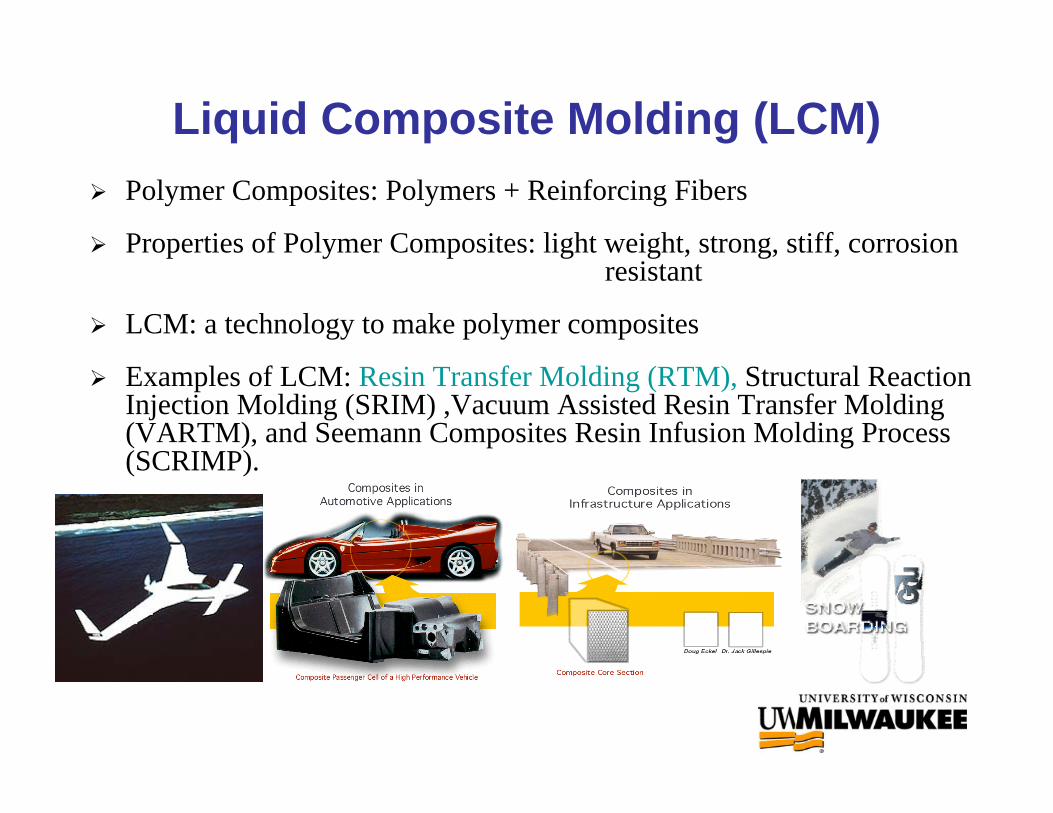
Liquid Composite Molding (LCM)Polymer Composites: Polymers + Reinforcing Fibers

Properties of Polymer Composites: light weight, strong, stiff, corrosion resistant

LCM: a technology to make polymer composites

Examples of LCM: Resin Transfer Molding (RTM), Structural Reaction Injection Molding (SRIM) ,Vacuum Assisted Resin Transfer Molding(VARTM), and Seemann Composites Resin Infusion Molding Process (SCRIMP).

1. Preform Manufacturing

2. Lay-up and Draping

3. Mold Closure

4. Resin Injection and Cure

5. Demolding and Final Processing

Process steps in Resin Transfer Molding (RTM)Process steps in Resin Transfer Molding (RTM)

Mold-Filling Simulation in RTM

Flow-front progress Temperature distribution

Mold fill-time

Mold-Filling Simulation in RTM

Resin Velocity Distribution

Passenger mini-van cross-member

Advantages of moldAdvantages of mold--filling simulation in RTMfilling simulation in RTM

Optimize location of inlet gates and vents

Monitor mold fill-time and cure

Predict pressure and temperature buildup in the mold

Study the effect of different fibrous reinforcements on filling

Flow through a porous medium: averaging of flow variablesFlow through a porous medium: averaging of flow variables

fiber

averaging volume

∫=V f

dVV

vq rr 1∫=V f

V fdVpp 1

Volume average: Pore average:

∫=V f

V fdVcc 1∫=

V f

dVTV

T1

( ) ( ) Dτ :++∇⋅∇=∇⋅+∂∂ T,cTkTvtT fHCC cRpp ρρρ r

where

( ) ( )[ ]vv Trr∇∇ +=

21D

Microscopic Energy Balance:

Dτ μ2=

Effects of averaging on balance equations in a porous mediuEffects of averaging on balance equations in a porous mediumm

(Incompressible, Newtonian fluid)

TbT̂wheredVbv̂V fV

Cf

pD ∇⋅=⎪⎭

⎪⎬⎫

⎪⎩

⎪⎨⎧−= ∫

rrr1ρεK

Macroscopic Energy balance

( ){ } =∇⋅+∂∂

+ TqtT

CCC psp prρρε ρε

( ){ } ( ) qqK

T,cT fH cRDerr⋅++∇⋅+⋅∇

μρεKk

⎪⎭

⎪⎬⎫

⎪⎩

⎪⎨⎧

−+⎪⎭

⎪⎬⎫

⎪⎩

⎪⎨⎧

+= ∫∫ dSbdSbV

kSS fsfs

nV

kn fss

ssfserr rr

εεε

ε 11 δδk

Effective thermal conductivity tensor

Dispersive thermal conductivity tensor

Effects of averaging on balance equations in a porous mediuEffects of averaging on balance equations in a porous mediumm

Conventional moldConventional mold--filling simulation physics for RTMfilling simulation physics for RTM

( ){ } ( )Tcccvtc f

c,εεε +∇⋅+⋅∇=∇⋅+

∂∂

DD Dfr

Mass balance 0=⋅∇ vr

Energy balance

( ){ } ( ){ } ( )TcfHTTvCtT

C p cRDepspC ,ρερρερε +∇⋅+⋅∇=∇⋅+∂∂

+ Kkr

Chemical reaction

Darcy’s Law pv ∇−=μKr 0=∇⋅∇ p

μK

Elliptic pressure equation

Real flow Simulation (FE/CV scheme)

Finite Element/Control Volume (FE/CV): 1) most widely used approach because its simplicity, efficiency and robustness. 2) circumvents the front-tracking related problems associated with the adaptive mesh

regeneration method by using an Eulerian fixed mesh.

Typical experiments to measure inTypical experiments to measure in--plane fiberplane fiber--mat permeabilitymat permeability

radial flow mold1-D flow mold

constant pressurefluid supply

constant injection-ratefluid supply

⎟⎟⎠

⎞⎜⎜⎝

⎛Δ

μ⎟⎠⎞

⎜⎝⎛=

PL

AQKpv ∇−=

μKr

1-D flow:

Experimental Investigation of the 1Experimental Investigation of the 1--D unsaturated flowD unsaturated flow

x

Mold and Flow DetailsMold and Flow Details

Direction of Flow

Modeling Flow Variables during Unsaturated Flow

Inlet pressure history for 1Inlet pressure history for 1--D constant injectionD constant injection--rate experimentrate experiment

Continuity:

Darcy’s law:

Front speed:

xx f

Pin

0x=

dud

uxdPd=−

μK

utd

d x f =ε

tKuPin ⎟

⎟⎠

⎞⎜⎜⎝

⎛=

εμ2

Pin

t

Flow-front and Inlet-Pressure prediction

for 1-D Flow: Random Fiber Mats

0 10 20 30 400

20000

40000

60000

80000

100000

120000

140000

Pre

ssur

e /P

a

Time/sec

Experimental

Theoretical

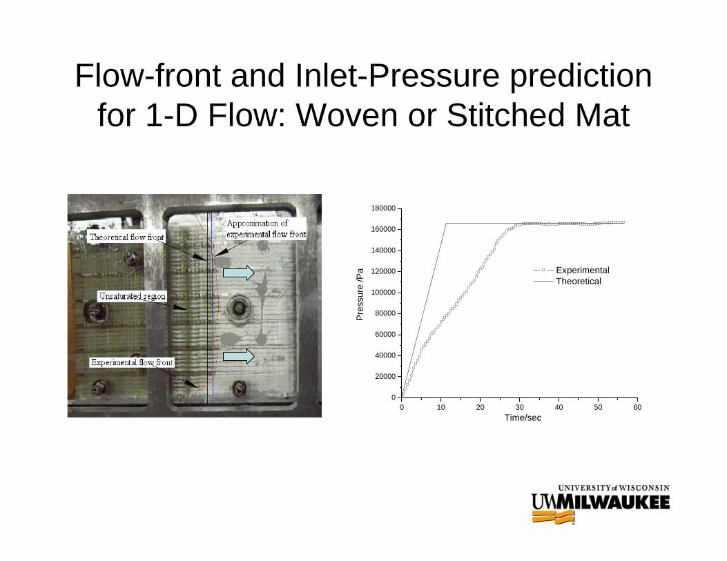
Flow-front and Inlet-Pressure predictionfor 1-D Flow: Woven or Stitched Mat

0 10 20 30 40 50 600

20000

40000

60000

80000

100000

120000

140000

160000

180000

Experimental Theoretical

Pres

sure

/Pa

Time/sec

Pin

t

rando

m mat

woven or stitched mat

Inlet pressure history: constant injectionInlet pressure history: constant injection--rate 1rate 1--D experimentD experiment

Pin

Droop

Random fiber matRandom fiber mat

One single fiber tow

Single-scale Porous Media

Woven and stitched fiber matsWoven and stitched fiber mats

Fibertows

Flow direction

Inter-tow spaces are absent

Li(Intra-tow

space)

Bi-axial woven mat

Dual-scale or dual-porosity media

Travel of a dark colored test liquid in a unidirectional stitched mat injected first with a

lighter color liquid

Courtesy: Prof. Lee, Ohio State University

Dry fiber matInitially injected light-colored liquid

Later injected dark-colored liquid

Radial Injection Pattern

Random Mat (Single-scale Porous Medium)

Biaxial Stitched Mat (Dual-Scale Porous Medium)

Two-Color Experiment: Random mat

Two-Color Experiment: Stitched mat

•``Experimental investigations of the unsaturated flow in Liquid Composite Molding'', T. Roy, C. Dulmes, and K.M. Pillai, Proceedings of the 5th Canadian-International Conference in Vancouver, Canada, August 16-19, 2005

Role of fiber bundles in creation of unsaturated flow and sink effect in woven/stitched fiber mats

Typical micrograph of an RTMpart made with stitched/woven

fiber mat

Schematic: absorption of resin by fiberbundles and creation of sink effect

Unsaturated flow in a simple, twoUnsaturated flow in a simple, two--layer modellayer model

Details of the Mesh and the Control Volumes Details of the Mesh and the Control Volumes

Inner CVs

Outer CVs

Finite difference scheme based on the control volumeformulation

x*

y*

0 0.1 0.2 0.3 0.4 0.5 0.6

0

1

2

3

4

T60.208457.693555.178652.663750.148947.63445.119142.604240.089337.574435.059532.544730.029827.514925

x*

y*

0 0.025 0.05 0.075 0.1 0.125

0

0.2

0.4

0.6

0.8

T48.378746.708845.038943.36941.699140.029238.359336.689435.019533.349531.679630.009728.339826.669925

Evolution of temperature distributionEvolution of temperature distribution

x*

y*

0 0.1 0.2 0.3

0

0.5

1

1.5

2

T56.252254.019951.787649.555347.32345.090742.858440.626138.393836.161533.929231.696929.464627.232325

t = 0.2 tch t = 4 tcht = tch

•“A Numerical Study of Non-Isothermal Reactive Flow in a Dual-Scale Porous Medium under Partial Saturation”, K.M. Pillai and R.S. Jadhav, Numerical Heat Transfer, Part A: Applications, 46: 1-28, 2004.

x*

y*

0 0.025 0.05 0.075 0.1 0.125

0

0.2

0.4

0.6

0.8

al0.0002268710.0002117460.0001966220.0001814970.0001663720.0001512470.0001361230.0001209980.0001058739.07485E-057.56237E-056.0499E-054.53742E-053.02495E-051.51247E-05

Evolution of cure distributionEvolution of cure distribution

x*

y*

0 0.1 0.2 0.3

0

0.5

1

1.5

2

al0.0009852540.0009195710.0008538870.0007882040.000722520.0006568360.0005911530.0005254690.0004597850.0003941020.0003284180.0002627350.0001970510.0001313676.56836E-05

x*

y*

0 0.1 0.2 0.3 0.4 0.5 0.6

0

1

2

3

4

al0.003983060.003717530.003451990.003186450.002920910.002655380.002389840.00212430.001858760.001593230.001327690.001062150.0007966130.0005310750.000265538

t = 0.2 tch t = tch t = 4 tch

Comparison of temperature predictions by the twoComparison of temperature predictions by the two--layer layer dualdual--scale model and the conventional singlescale model and the conventional single--scale modelscale model

x*

T*,θ

*,τ

0 .0 5 0 .10

0 .0 5

0 .1

0 .1 5

0 .2

0 .2 5

0 .3

0 .3 5

0 .4

θ * fo r d u a l sca le m o d e lT * fo r d u a l sca le m o d e lτ fo r s in g le sca le m o d e l

x

VolumeVolume--averaging in a dualaveraging in a dual--scale porous mediascale porous media

dVΒVΒ gVg

g ∫=><1

dVΒV

Β gVgg

gg ∫=><

1

dVnΒVΒΒ gtgAgt

gg ∫+><∇=>∇<1

dVΒVΒttΒ

gtgAgt

gg nu ⋅−><

∂∂

=>∂∂

< ∫1

Averaging Theorems

(Pillai & Murthy, 2004)

Governing equations for reactive, Governing equations for reactive, nonisothermalnonisothermal,,unsaturated flow in dualunsaturated flow in dual--scale porous mediascale porous media

Sg −=><⋅∇ v ><∇−=>< ggg P

Kμ

v

QQfHTTtT

C condconvcRggg

gthg

gg

gg

gp l−++∇⋅⋅∇=

⎥⎥

⎦

⎤

⎢⎢

⎣

⎡∇⋅><+

∂

∂><><><

ρεερ Kv)(

MMfcctc

diffconvcgg

gg

gg

gg

g −++∇⋅⋅∇=∇⋅><+∂

∂><><><

εε Dv

Mass Balance: Momentum Balance:

Energy Balance:

Cure Balance:

Various source and sink terms:dA

AVS gtg

gt

nv ⋅= ∫1

dAAV

Q gtgcondgt

nq ⋅= ∫1

⎥⎦⎤

⎢⎣⎡ ><−><= TTSCQ g

gtg

ggpgconv ,ρ ⎥⎦

⎤⎢⎣⎡ ><−><= ccSM g

gtg

gconv

dAAVM gtgdiffgt

nJ ⋅= ∫1

(Pillai & Murthy, 2004)

Coupled macroCoupled macro--micro approach for modelingmicro approach for modelingthe unsaturated flowthe unsaturated flow

•“Governing equations for unsaturated flow through woven fiber mats, Part 2: Nonisothermal reactive flows”, K.M. Pillai and M.S. Munagavalsa, Composites Part A: Applied Science and Manufacturing, v 35, 2004, p403-415.

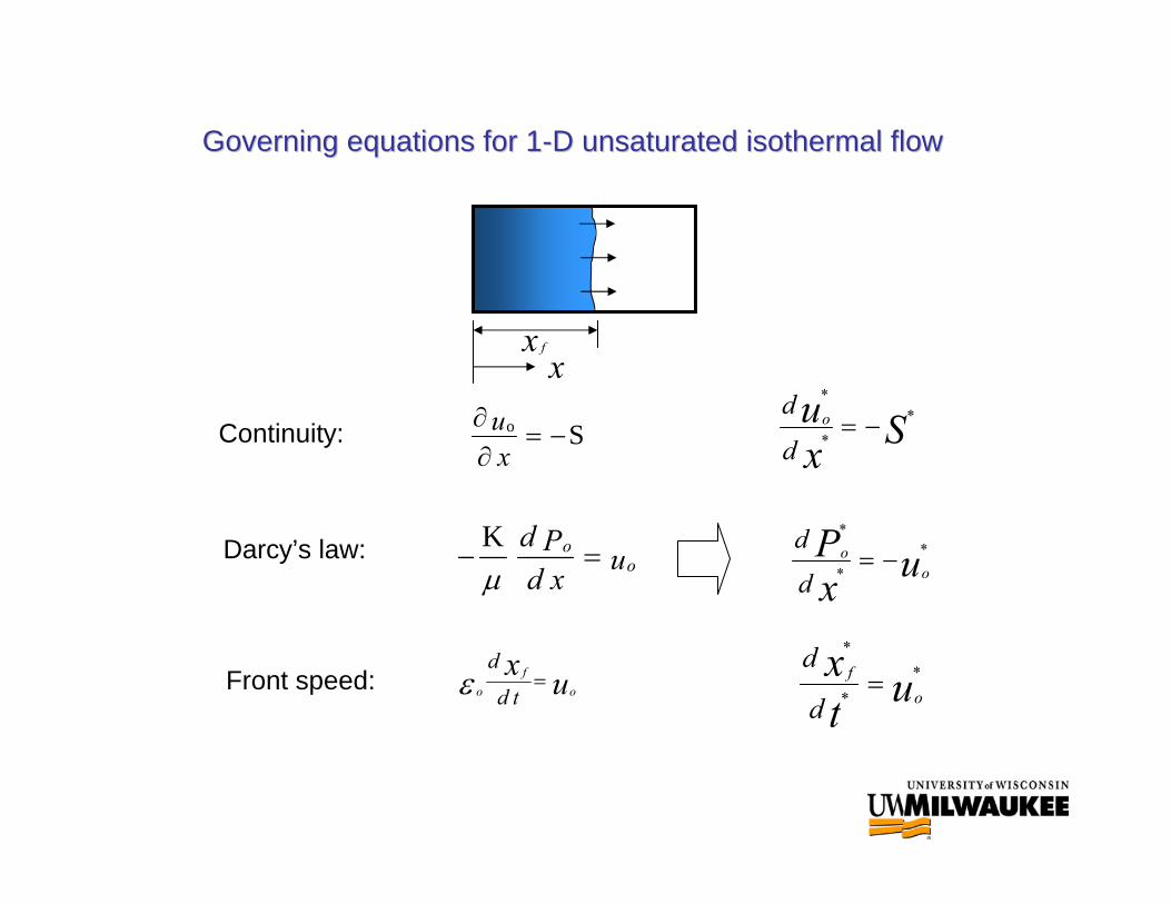
Governing equations for 1Governing equations for 1--D unsaturated isothermal flowD unsaturated isothermal flow

Continuity: So −=∂∂xu Sx

ud

do ∗

∗

∗

−=

Darcy’s law: uxdPd

oo =−

μK

uxP

oo

d

d ∗

∗

∗

−=

Front speed: uxo

fo td

d=ε ut

xo

f

d

d ∗

∗

∗

=

xx f

Inlet pressure history for the constant sink caseInlet pressure history for the constant sink case

SeP

tSin 2

21∗

−∗

∗∗−

=

Previous ExperimentsPrevious Experiments

Governing EquationsGoverning EquationsConstant injectionConstant injection--rate radial flowrate radial flow

Sru

ru oror

d

d ∗

∗

∗

∗

∗

−=+

urP

oro

d

d ∗

∗

∗

−=

utr

orf

d

d ∗

∗

∗

=

Inlet pressure history for the radial flow (analytical sInlet pressure history for the radial flow (analytical solution)olution)

Modeling Bubble Creation & Migration during Unsaturated

Flow

Bubble Creation and Migration

• Numerous studies on Bubbles or Voids in RTM

• Bubbles created due to mechanical trapping of air pockets in porous media during mold filling

• Bubble creation due to evaporation of volatile compounds in resin is insignificant

• Capillary number plays an important role in deciding the type of bubble created

0.1 1.00.010.0010.0001

% v

olum

e of

voi

ds

% v

olum

e of

voi

ds

Macrovoids Microvoids

5

10 10

5

Void trapping mechanisms & its dependence on Capillary Number

CaCa V

Cos= μσ θ

Patel, Lee et al.

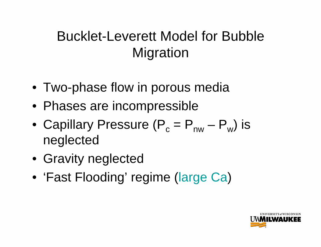
Bucklet-Leverett Model for Bubble Migration

• Two-phase flow in porous media• Phases are incompressible• Capillary Pressure (Pc = Pnw – Pw) is

neglected• Gravity neglected• ‘Fast Flooding’ regime (large Ca)

Bucklet-Leverett Formulation0)( =⋅∇+∂ rrt qS rφ

0)( =⋅∇+∂ aat qS rφ

1=+ ra SS

Mass Balance:

Generalized Darcy’s Law:PKkq

rrrelr ∇=μ,

r

PKkqa

arela ∇=μ,

r

Bucklet-Leverett Equation

where

1-D Flow

ar

r

qqqr+

= = fractional flow rate

1st order Quasi-linear Hyperbolic Equation

0=∂∂

+∂∂

xSU

tS rr

r

ar

SdrdqqU

ε+

= = signal speed

Bucklet-Leverett Model for Bubble Migration

t1

t2

t3

t3 > t2 > t1

(Sr)

0

0.2

0.4

0.6

0.8

1

0 5 10 15 20 25 30 35 40 45 50

br1t> 2 >

2

t3t

t 31

Sr

x(nodes)

t t

Typical Pattern of Bubble Migration(Lundstrom & Gebart)

Buckley-Leverett Saturation Fronts (Pillai & Advani )

Buclet-Leverett Model: Void Distribution from Numerical Simulation

)(1)(

,

,, PS

PSSS

resida

residaareda −

−=If P > Pcritical, then air bubble moves

(Chui & Glimm et al.)

Bucklet-Leverett Model for Bubble Migration

• Lundstrom, T.S. & Gebart, B.R., Influence of Process Parameters on Void Formation in Resin Transfer Molding, Polymer Composites, 15(1):25-33, Feb. 1994

• Pillai, K.M. & Advani, S.G., Modeling of Void Migration in Resin Transfer Molding, Proceedings of 1996 IMECE(ASME), page 14, 1996.

• Chui, W.K., Glimm, J., Tangerman, F.M., Jardine, A.P., Madsen, J.S., Donnellan, T.M., and Leek, R., Process Modeling in Resin Transfer Molding as a Method to Enhance Product Quality, SIAM Rev., 39(4):714-727, Dec 1997.

Conventional 2-Phase Flow Models to Predict Void Distribution/Saturation during Slow (small

Ca) 1-D Flows

Experimentally Measured Saturation Distribution

Numerically predicted saturation

• Breard et al. “Numerical Simulation of void Formation in LCM”, Composites: Part A 34 (2003) 517-523

Challenge of Unified theory for flow and Bubble/Void during Unsaturated

Flow

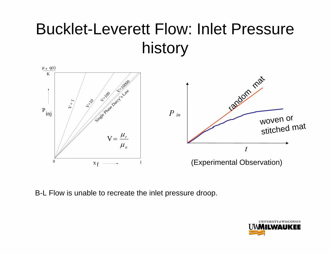
Bucklet-Leverett Flow: Inlet Pressure history

Pinj

μ r q(t)

K

x f

V=1000

0

V=100

V=1

0

V =

1

Single

Phase

Darc

y’s L

aw

0 1

a

r

μμ

=V

P in

t

rando

m mat

woven or

stitched mat

B-L Flow is unable to recreate the inlet pressure droop.

(Experimental Observation)

Unification of Flow Variable & Bubble Creation/Migration Predictions during RTM mold filling

Simulation involving `sink’ model for dual-scale porous media recreate the pressure droop during high Ca flow, but is unable to predict bubble creation/migration.

Buclet-Leverett type formulations can predict bubble creation/migration during high Ca flow, but are unable to recreate the pressure droop

Conventional 2-phase flow formulations have been tried to model low Ca flows, but are unable to recreate the pressure droop.

Unification of Flow Variable & Bubble Creation/Migration Predictions during RTM mold filling

(Cont’d)

Numerical, algorithmic approach: FE/CV formulation for modeling flow; use of line elements attached to FE nodes to model `sink’ like disappearance of fluid; saturation = 1 as P > Pcrit. Example: LIMS of U. of Delaware

Several problems: possible inaccuracy in physics; ad-hoc approach; temperature and cure modeling absent; weak experimental validation.

Challenge of developing a comprehensive continuum model still unmet.

Summary

Unsaturated flow fundamentally different in single-scale and dual-scale fiber mats.

`Sink’ model developed to model the unsaturated flow in dual-scale porous media.

Both low and high Ca flows can be modeled using 2-phase approach to predict saturation (bubble) distribution. However recreation of inlet pressure droop not achieved for dual-scale media.

Challenge: a need for a comprehensive continuum model for predicting pressure/velocity and saturation/bubbles

Thank you for your attentionQuestions ?

Permeability Estimation in

Fibrous Porous Media

Polymer Processing Laboratory

pKu ∇−= .η

⎟⎟⎟

⎠

⎞

⎜⎜⎜

⎝

⎛

=

ZZZYZX

YZYYyx

XZXYxx

kkk

kkkkkk

K

⎟⎟⎟⎟⎟⎟⎟

⎠

⎞

⎜⎜⎜⎜⎜⎜⎜

⎝

⎛

∂∂∂∂∂∂

⎟⎟⎟

⎠

⎞

⎜⎜⎜

⎝

⎛

−=⎟⎟⎟

⎠

⎞

⎜⎜⎜

⎝

⎛

zpypxp

kkk

kkkkkk

u

uu

ZZZYZX

YZYYyx

XZXYxx

z

y

x

η1

If the selected coordinate directions are along the principal directions, we have

⎟⎟⎟⎟⎟⎟⎟⎟

⎠

⎞

⎜⎜⎜⎜⎜⎜⎜⎜

⎝

⎛

∂∂∂∂∂∂

⎟⎟⎟

⎠

⎞

⎜⎜⎜

⎝

⎛−=

⎟⎟⎟

⎠

⎞

⎜⎜⎜

⎝

⎛

3

2

1

33

22

11

3

2

1

0000

001

xpxpxp

kk

k

uuu

η

Tensor nature of the Permeability

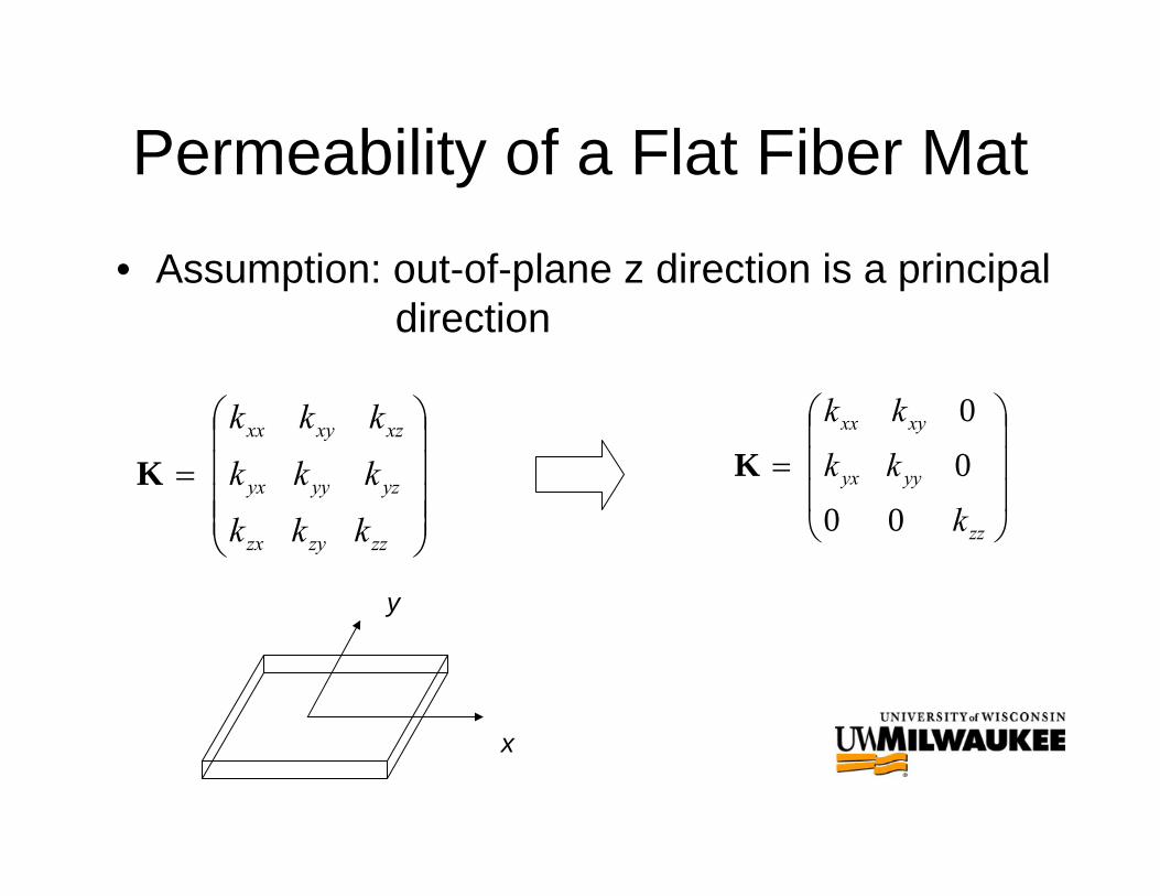
Permeability of a Flat Fiber Mat

• Assumption: out-of-plane z direction is a principal direction

⎟⎟⎟⎟

⎠

⎞

⎜⎜⎜⎜

⎝

⎛

=

zzzyzx

yzyyyx

xzxyxx

kkk

kkk

kkk

K⎟⎟⎟

⎠

⎞

⎜⎜⎜

⎝

⎛

=

zz

yyyx

xyxx

k

kk

kk

00

0

0

K

x

y

Typical experiments to measure inTypical experiments to measure in--plane fiberplane fiber--mat permeabilitymat permeability

radial flow mold1-D flow mold

constant pressurefluid supply

constant injection-ratefluid supply

Permeability measurement through 1-D Channel Flow

Resin inlet

⎟⎟⎠

⎞⎜⎜⎝

⎛Δ

μ⎟⎠⎞

⎜⎝⎛=

PL

AQKpv ∇−=

μKr

Isotropic Medium:

In-plane Permeability Tensor for Anisotropic Fiber Mats

⎥⎦

⎤⎢⎣

⎡=

yyyx

xyxx

KKKK

K ⎥⎦

⎤⎢⎣

⎡=

2

1

00K

KK

θ2/1 CosDADAKK I −

−=

, y

45o

III

I , x

1

2 II

θ

θ2/2 CosDADAKK III +

+=

⎟⎟⎠

⎞⎜⎜⎝

⎛−

−= −

DA

DKDA

II

221tan

21θ

2IIII KKA +

=

2IIII KKD −

=

where

1-D Flow Permeability Measuring Process

Advantages

• Simpler physics

• Easier data analysis

• Low mold deflection

Disadvantages

• Sliding of Fiber Mats

• Increased flow on the side edges (race-tracking)

• Three experiments for anisotropic fiber mats

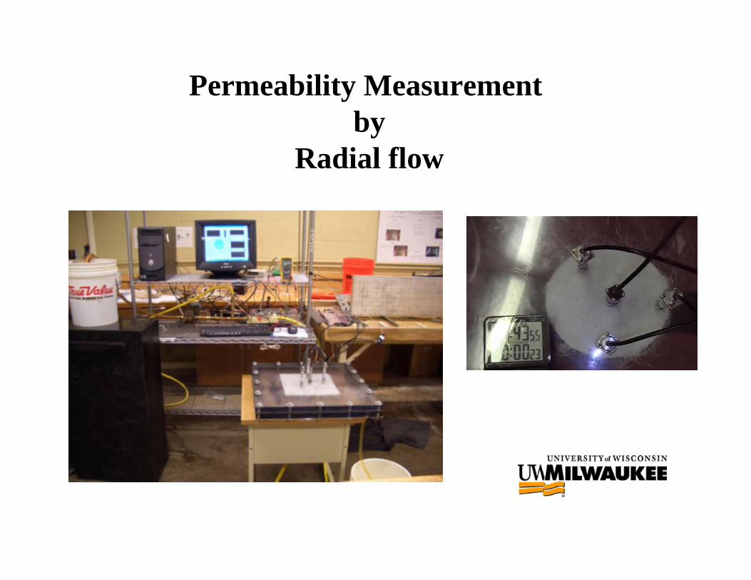
Permeability Measurementby

Radial flow

Permeability tensor measured through transient radial flow

x

y

12

Flow front position

1 and 2 are two principal directions

In a constant flow-rate experiment, the flow front positions and inlet pressure are functions of time [1,2]. The in-plane permeability tensor can be expressed as

⎥⎦

⎤⎢⎣

⎡=

2

1

00K

KK

Based on the Darcy’s law and continuity equation, the effective permeability can be expressed as

⎥⎦

⎤⎢⎣

⎡+== f

rR

hPQKKK f

ineff ln)ln(

2 0

121 π

μ

Injection port r0

where

1

111

2

1

2

12

1

20

+

⎟⎟⎠

⎞⎜⎜⎝

⎛−++

=

KK

KK

Rr

f f 2

1

2

1

KK

RR

f

f =

where R1f and R2f are the radial flow front along the principal directions, respectively; r0 is the inlet port radius, K1 and K2 are principal permeabilities. 1. Adams, K.L.,etc. Forced in-plane flow of an epoxy resin in fibrous networks. Polym. Eng. Sci. 1986, 26(20),1434.

2. Chan, A.W., Hwang Sun-Tak, Anisotropic in-plane permeability of fabric media. Polym. Eng. Sci. 1991, 31(16),1233.

Permeability tensor measured through transient radial flow (Cont.)

Data analysis procedure1. the ratio α(K1/K2) can be determined by flow visualization. While the flow

pattern forms a fully developed ellipse, the degree of anisotropy α of the flow pattern can be expressed as

2. Since Q, μ, and h are known, we have the following equation

where m can be obtained from the slope of the curve Pin versus (ln(R1f /r0)+lnf ).

3. The values of K1 and K2 are then calculated from the relations:

2

2

12

⎟⎟⎠

⎞⎜⎜⎝

⎛=⎟⎟

⎠

⎞⎜⎜⎝

⎛=

f

f

RR

axisellipticminoroflengthaxisellipticmajoroflengthα

mhQKKKeff

1221 πμ

==

effKK α=1α

effKK =2

Permeability tensor measured through steady-state radial flow

• a steady-state radial flow experiment is developed to measure permeability[3]. In this method, pressures at four locations in the flow field, instead of flow front locations, are measured and used for determining the permeabilities.Two equations are used to find the permeability tensor the preform.

P1

P2

P3

X

Y

R=3”

P0θ=1200

1

2 β

positions of pressure transducers

( )( ) 02

1

1log111

11log 10

21

21

0

1

2

0

1 =−

−⎟⎟⎟

⎠

⎞

⎜⎜⎜

⎝

⎛

−

+−

⎥⎥

⎦

⎤

⎢⎢

⎣

⎡

−+−⎟⎟

⎠

⎞⎜⎜⎝

⎛

−effK

Qpph

xx

xx

μπ

α

ααα

( )( ) 02

1

1log1

11

log 20

21

21

0

2

2

0

2 =−

−⎟⎟⎟

⎠

⎞

⎜⎜⎜

⎝

⎛

−

+−

⎥⎥

⎦

⎤

⎢⎢

⎣

⎡

−++⎟⎟

⎠

⎞⎜⎜⎝

⎛

−effK

Qpph

yy

yy

μπ

α

αα

αα

α

where (x0, y0), (x1, y1) and (x2, y2) are the coordinates of points P0, P1, and P2 respectively. Q is the flow rate; h is the mold gap thickness.

3. K. Ken Han, etc. (2000) Measurements of the permeability of fiber preforms and applications, Composites Science and Technology, 60 (12-13): 2435-2441.

Permeability tensor measured through steady-state radial flow (Cont.)

• After plugging the steady-state pressure values into these two non-linear equation, one can solve for the degree of anisotropy α and Keff . The principal permeabilities K1 and K2 through relations α = K1/K2 and β is the angle between the principal axis and lab coordinates X-Y as shown in the figure and can be estimated by plugging the third pressure P3 into a coordinate transformation equation.

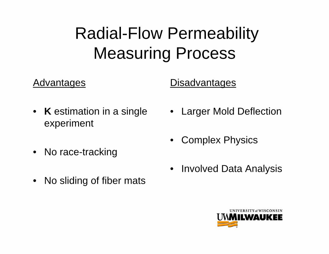
Radial-Flow Permeability Measuring Process

Advantages

• K estimation in a single experiment

• No race-tracking

• No sliding of fiber mats

Disadvantages

• Larger Mold Deflection

• Complex Physics

• Involved Data Analysis

Calibration Devices for Permeability Measuring Setup

1) A method to estimate the accuracy of radial flow based permeability measuring devices,Hua Tan and Krishna M. Pillai, to appear in Journal of Composite Materials.

2) A method to estimate the accuracy of 1-D flow based permeability measuring devicesHua Tan, Tonmoy Roy and Krishna. M. Pillai, Journal of Composite Materials, 2007.

Radial Flow 1-D Flow

Theoretical Models

for

Permeability of Fiber Beds

Permeability Models• There are many permeability models that has been proposed so far. The

simplest model is to consider the porous medium as a bundle of capillaries [4]. The model takes the general form of

where Ø is porosity, is tortuosity, and Av is surface area per unit volume. Since the determination of tortuosity is arbitrary, this makes the model difficult to apply.

• Another capillary model is the network model in which a multitude of capillaries are arranged in the form of a regular network [5]. The well-known Kozeny-Carman equation is based on this approach

where C is Kozeny-Carman equation

vAK 22

3

τφ

=

τ

22

3

)1( φφ−

=vCA

K

4. L. Skartsis,etc. Resin flow through fiber beds during composite manufacturing processes, Polymer Engineering and Science, 32, 221,1992

5. Lenormand, etc. Mechanisms of the displacement of one fluid by another in a network of capillary ducts. Journal of Fluid Mechanics, 135, 337, 1983.

Permeability Models• Basing on the Kozeny-Carman equation, many researchers propose the

following permeability model for flow along the fiber direction [6]

where Kx is the permeability in the fiber direction, rf is the fiber radius, Cis the Kozeny constant to be determined experimentally, and Vf is the fiber volume fraction.

• For flow transverse to the fiber bundle, Gutowski [7] proposed relation is

Where Kz is the permeability along the transverse direction, Va is the available fiber volume fraction at which the transverse flow stops. The constant C was measured experimentally and was found to be 0.2, and Va was determined to be around 0.8-0.85.

( )2

32

41

f

ffx VC

VrK

−=

( )( )14

132

+′

−′=

fa

fafz VVC

VVrK

6. Williams, J.G., etc., Liquid flow through aligned fibre beds. Polymer Engineering and Science, 14, 413, 1974.

7. Gutowski, T.G. etc, Consolidation experiments for laminate composites. Journal of composite materials, 21, 7, 650, 1987.

Permeability Models

• Gebart [8] assumed that most of the flow resistance is concentrated in the narrow gaps between adjacent fibers, therefore developed an analytical model to estimate the permeability. The permeability for quadratic and hexagonal arrangement of fibers can be written as

The parameters B1, B2, and Vf,max depend on the fiber arrangement.

( )2

1

32 18

f

ffx VB

VrK

−=

2

25

max,2 1 f

f

fz r

VV

BK ⎟⎟⎠

⎞⎜⎜⎝

⎛−=

8. Gebart, B.R. Permeability of unidirectional reinforcements for RTM. Journal of Composite Materials, 26(8), 1100, 1992

Permeability-estimating model (Cont.)

• Another approach is the self-consistent method. This method assumes that a unit cell of a heterogeneous medium can be considered as being embedded in an equivalent homogeneous media whose properties are unknown and to be determined [9]. Theflow inside the unit cell satisfies Navier-Stokes equation, while the flow outside of the unit cell follows Darcy’s law. The consistency conditions are that the total amount of the flow and the dissipation energy remain the same with and without this insertion of unit cell.

( )( )⎥⎥⎦

⎤

⎢⎢⎣

⎡−−−= ff

ff

fx VV

VVr

K 131ln8 2

2

⎥⎥⎦

⎤

⎢⎢⎣

⎡

+

−−= 2

22

111ln

8 f

f

ff

fz V

VVV

rK

9. Berdichevsky, A. and Cai, Z. Preform permeability predictions by self-consistent method and finite elements simulation, Polymer composites, 14(2), 132, 1993.

Thank you for your attention.

Questions ?

Wicking of Liquids into

Fibrous Porous Media

Polymer Processing Laboratory

Physics Behind Wicking

SLSGGL Cos σσθσ −=

G

L

S

Young’s Equation

θL

o90<θ

Wetting

θL

o90>θ

Non-Wetting

Wicking across a Fiber-bank

•``Wicking across a Fiber-bank'', K. M. Pillai and S. G. Advani, Journal for Colloid and Interface Science, v 183, no.1, 1996, p100-110.

Modeling MicroModeling Micro--Flow inside the Fiber BankFlow inside the Fiber Bank

h

Suction PressureNon-dimensional suction pressure

• Energy model

• Ahn et. al. model

• Williams et. al. model

⎟⎟⎠

⎞⎜⎜⎝

⎛=

fss dPP )cos(4/ θγ

fs vP =

)1(4 f

fs v

vP

−=

f

fs v

vP

−=

1

Measuring Wicking ParametersLiquid parameters:• Density• Viscosity • Surface Tension

Porous media parameters:• Porosity• Permeability • Fiber diameter

Liquid-solid interaction• Contact angle

Rheometer

DCA

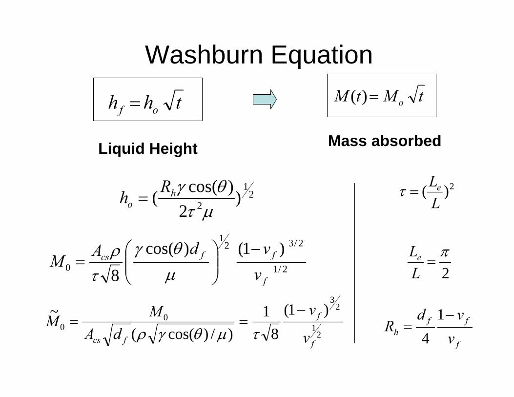
Washburn Equation

21

2 )2

)cos((μτθγh

oRh =

2)(LLe=τ

2π

=LLe

f

ffh v

vdR

−=

142

1

23

00

)1(8

1)/)cos((

~

f

f

fcs v

vdA

MM−

==τμθγρ

thh of =tMtM o=)(

2/1

2/321

0

)1()cos(8 f

ffcs

vvdAM

−⎟⎟⎠

⎞⎜⎜⎝

⎛=

μθγ

τρ

Mass absorbedLiquid Height

Darcy’s Law based Model for Wicking

tMtM o=)(

sf

cs KPv

AMμ

ρ)1(2

0

−=

Liquid Mass wicked into Fiber Bank

Motor Oil

Experiments with different Liquids

tMtM o=)(

Mineral oil

Glycerine Motor oil

Silicon oil

Effectiveness of Models

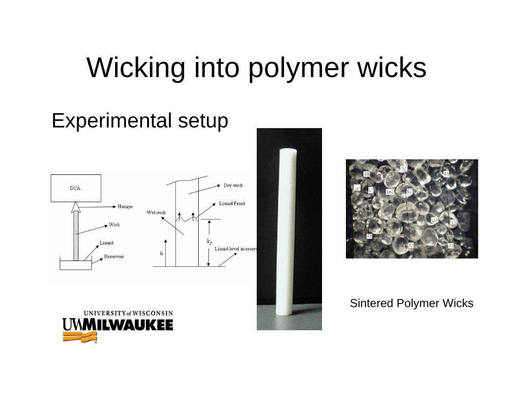
Wicking into polymer wicks

Experimental setup

Sintered Polymer Wicks

Comparing Models with Test Data

0

0.1

0.2

0.3

0.4

0.5

0.6

0.7

0.8

0.9

0 10 20 30 40 50 60 70 80

t [s]

m [g

]

Test ResultsCapillary ModelE.B. Model with gravityCapillary Model with gravityE.B. ModelWashburn Model

Polycarbonate Wick

and Liquid Decane

0

0.2

0.4

0.6

0.8

1

1.2

1.4

1.6

1.8

0 20 40 60 80 100 120

t [s]

m [g

]

Test ResultsCapillary ModelE.B.Model with gravityCapillary Model with gravityE.B. ModelWashburn Model

Polypropylene Wick

and Liquid Hexadecane

• “Darcy’s Law based Models for Liquid Absorption in Polymer Wicks,” by Reza Masoodi, Krishna M. Pillai, P. Varanasi, to appear in AIChE Journal.

Thank you for your attention.

Questions ?