Flexion and Skewness in Map Projections of the Earth

David M. Goldberg (Drexel University Dept. of Physics)

J. Richard Gott III (Princeton University Dept. of Astrophysical Sciences)

goldberg@drexel.edu, jrg@astro.princeton.edu

April 11, 2007

Abstract

Tissot indicatrices have provided visual measures of local area and isotropy distortions.

Here we show how large scale distortions of flexion (bending) and skewness (lopsidedness) can

be measured. Area and isotropy distortions depend on the map projection metric, flexion and

skewness, which manifest themselves on continental scales, depend on the first derivatives of

the metric. We introduce new indicatrices that show not only area and isotropy distortions

but flexion and skewness as well. We present a table showing error measures for area, isotropy,

flexion, skewness, distances, and boundary cuts allowing us to compare different world map

projections. We find that the Winkel-Tripel projection (already adopted for world maps by the

National Geographic), has low distortion on most measures and excellent quality overall.

Keywords: Maps, Earth, Projection, Curvature

1 Introduction

Tissot (1881) indicatrices have been very useful for providing a visual presentation of local dis-

tortions in map projections in a simple and compelling fashion. A small circle of tiny radius (say

1

0.1 degree of arc in radius) is constructed at a given location, and then enlarged and projected

on the map at that location. This always produces an ellipse. Usually one favors conformal map

projections that minimize the changes in scale factor, or equal area projections that minimize

anisotropy, or recently, map projections that are neither conformal nor equal area, but which have

a judicious combination of minimizing both scale and isotropy errors (like the Winkel-tripel used

by the National Geographic Society for world maps).

The Tissot ellipse at a given location is specified by three parameters, the major axis, the minor

axis, and the orientation angle θ of the major axis of the ellipse. Geometrically, from differential

geometry (and General Relativity) we know that the measurement of local distances is measured

by the metric tensor gab, where a and b can each take the values x or y, yielding three independent

components. Locally for two nearby points separated by infinitesimal map coordinate differences

dx and dy, the true distance between these two points on the globe is given by:

ds2 = gxxdx2 + 2gxydx dy + gyydy2 (1)

The Tissot ellipse (major axis, minor axis, and orientation angle, θ) can be calculated from the

three components of the metric tensor. Thus, the Tissot ellipse essentially carries the information

on the metric tensor for the map. It tells us how local infinitesimal distances on the map correlate

with local infinitesimal distances on the globe.

As we will see, however, the Tissot ellipse does not carry all of the information related to

distortions, which has been noted previously. Others (Stewart 1943; Peters 1975, 1978; Albinus

1981; Canters 1989, 2002; Laskowski 1997ab) have noted that there are finite distortions apart from

those of the Tissot ellipse.

Previous authors have previously depicted finite size distortions by several methods, includ-

2

ing showing faces on a globe (Reeves 1910; Gedymin 1946), 30 degree x 30 degree equiangular

quadralaterals (Chamberlin 1947), a net of twenty spherical triangles, in an icosahedral arrange-

ment (Fisher & Miller 1944), 150 degree great circle arcs, and circles of 15 degrees radius Tobler

(1964).

In the Oxford Hammond Atlas of the World (1993) , new conformal map projections (”Ham-

mond Optimal Conformal Projections”) were designed for the continents. Following the Chebyshev

criterion (Snyder 1993), the rms scale factor errors were minimized by producing a constant scale

factor along the boundary of the continent. (For a circular region this conformal map would be

a stereographic projection.) By tailoring the boundary to the shape of each continent, the errors

could be reduced relative to those in a simple stereographic projection. In touting the advantages

of their projection the Hammond Atlas did the following experiment. Following Reeves (Reeves

1910), they constructed a face on the globe with a triangular nose, a straight (geodesic) mouth,

and eyes that were pairs of concentric circles on the globe. They then showed this face with various

map projections. In the gnomonic, the mouth was straight, but the eye circles were not circular

and were not concentric (what we would call skewness). The Mercator projection had the mouth

smiling (what we would call flexion) and although the eyes were circular they were not concentric.

The Hammond Optimal Conformal projections did a bit better on these qualities because the gra-

dients of the scale factor changes were small so the flexion and skewness were small, although of

course not zero.

In Sec. 2 we introduce the concept of “flexion”, by which a map projection can cause artificial

bending of large structures. In Sec. 3, we show another distortion: skewness, which represents

lopsidedness and an asymmetric stretching of large structures. We show a simple way to visualize

these distortions in Sec. 4, in which we introduce the “Goldberg-Gott Indicatrices.” In Sec. 5 we

derive a differential geometry approach to measuring flexion and skewness. While readers interested

3

in computing flexion and skewness on projections not included in this paper should refer to Sec. 5,

it is highly technical, and those interested in seeing results may skip directly to Sec. 6, in which

we discuss Monte Carlo estimates of the distortions for a number of projections, a ranking of map

projections, and our conclusions.

2 First Distortion: Flexion

The local effects shown by the Tissot Ellipse are not the only distortions present in maps. There

are also “flexion” (or bending) and “skewness” (or lopsidedness; discussed in the next section),

which describe curvature distortions visible on world maps (the terminology stems from a similar

effect in gravitational lensing; Goldberg & Bacon 2005).

One can think about flexion in the following way. Imagine a truck going along a geodesic of

the globe at unit angular speed (say one radian per day). Now imagine the image of that truck

on the map, moving along. If the map were perfect, if it had zero flexion and zero skewness, then

that truck would move in a straight line on the map with constant speed. Its velocity vector on

the map:

v =dx

dτ, (2)

would be a constant, where τ is the angle of arclength in radians traveled by the truck along the

geodesic on the globe. Its acceleration:

a =dv

dτ(3)

would be zero. Of course, this cannot be true for a general geodesic. In the general case, the

image of the truck suffers an acceleration as it moves along. The acceleration vector, a, in the

two-dimensional map has two independent components: a⊥ (which is perpendicular to the truck’s

velocity vector at that point), and a‖ (which is parallel to its velocity vector at that point).

4

The perpendicular acceleration, a⊥, causes the truck to turn without changing its speed on the

map. This causes flexion, or bending, of geodesics. We define the flexion along a given geodesic at

a given point to be:

f =a⊥v

, (4)

or, more usefully:

f =dv⊥dτ

1

v. (5)

In this form, we may define:

dα =dv⊥v

. (6)

where α is the angle of rotation suffered by the velocity vector. Remember, if a⊥ is the only

acceleration present, then the velocity vector of the truck on the map does not change in magnitude,

but just rotates in angle. Thus f = dα/dτ , and represents the angular rate at which the velocity

vector rotates divided by the angular rate at which the truck moves on the globe.

Skewness and flexion only express themselves on large scales. They are not noticeable on

infinitesimal scales where the metric contains all the information one needs, but become noticeable

on finite scales, with their importance growing with the size of the area being examined. Flexion

and skewness are thus important on continental scales and larger in a world map.

It is possible to design a map projection that has zero flexion: the gnomonic projection shows

all great circles as straight lines. However it does exhibit anisotropy, scale changes, and skewness,

and at best can show only one hemisphere of the globe.

2.1 Example 1: The Stereographic Projection

As an example, consider a truck traveling on the equator as seen by in the polar stereographic

projection (see Fig 1). In the stereographic projection, the north pole is in the center of the map

5

and the equator is a circle around it. As the truck circles the equator (the equator is a geodesic-so

the truck drives straight ahead on the globe), it travels around a circle on the map. By azimuthal

symmetry, the truck circles the equatorial circle on the map at a uniform rate. The velocity vector

of the truck on the map rotates a complete 360◦ (2π radians), as the truck circles the equator,

traversing 360◦ of arc on the globe. So the flexion is f = 1, for a point on the equator, for a geodesic

pointing in the direction of the equator. The flexion is defined at a point, and for a specific geodesic

traveling through that point.

For an arbitrary point on the equator in the stereographic projection and a geodesic pointing in

the direction of a meridian of longitude (also a geodesic) the flexion is zero, because these geodesics

are shown as radial straight lines in the polar stereographic projection, and the velocity vector of

the truck does not turn as it travels north.

The stereographic projection has the property that every great circle (geodesic) on the globe is

shown as a circle on the map, except for a set of measure zero that pass through the north pole

(i.e. the meridians of longitude). Thus by the argument given above, the average flexion integrated

around a random great circle must be 〈f〉 = 1, because the truck’s velocity vector on a random

great circle must rotate by 360◦ as it circles the 360◦ of arc completing that great circle on the

globe. The magnitude of the velocity vector of the truck on the map is larger the further from the

north pole it is and so its rotation per angle of arc of truck travel on the globe is larger there as

well, and so the flexion along that random geodesic is larger the further away from the pole one is,

with the integrated average value along the whole great circle being 〈f〉 = 1.

2.2 Example 2: The Mercator Projection

The Mercator projection (see Fig 2) is conformal and so only the scale factor changes as a function

of position on the map (i.e. gxx = gyy, and gxy = 0 and the Tissot ellipses are all circles with radii

6

proportional to 1/gxx). But there is bending. The northern boundary between the continental

United States and Canada at the 49th parallel of latitude is shown as a straight line in the Mercator

Map, but really it is a small circle that is concave to the north. If one drove a truck down that

border from west to east, one would have to turn the steering wheel slightly to the left so that one

was continually changing direction. The great circle route (the straightest route) connecting the

Washington State and Minnesota (both at the 49th parallel) is a straight line which goes entirely

through Canada. This straight line on the globe when extended, passes south of the northern part

of Maine, so the continental United States is bend downward like a frown in the Mercator Map.

(See Figure 3 and 4). Likewise, Maine on a Mercator map Maine sags below the line connecting

Washington State and Minnesota, while on the globe this is not true.

In the Mercator projection, the flexion along the equator is zero, also along all meridians of

longitude, but these are a set of measure zero. A random geodesic is a great circle that is inclined

at some angle between 0◦ and 90◦ with respect to the equator. On the Mercator map this is a wavy

line that bends downward in the northern hemisphere, and by symmetry, upward in the southern.

Since the curvatures are equal and opposite in the two hemispheres, the average flexion 〈f〉 = 0,

but this is misleading because the flexion at each point off the equator is not zero. So if we are

rating map projections by the amount of flexion they contain we should use the absolute value of

the flexion instead: |f |. In a region where the flexion does not change sign (such as the northern

hemisphere in the Mercator projection or the entire stereographic map) the total bending of a

geodesic segment will be the integral of the flexion |f | over that segment. In fact, in Section 6.1

we will evaluate the overall flexion on a map by simply picking random points on the sphere and

random directions for geodesics going through them, and then calculating the absolute value for

the flexion for all random points on the globe and random directions through them.

7

2.3 A Global Flexion Measure

We can calculate the flexion for any point in the Mercator (or any other) projection through any

geodesic using spherical trigonometry. As a reminder to the reader, the Mercator projection uses

the mapping:

x = λ (7)

y = ln (tan[π/4 + φ/2])

(8)

where here and throughout, λ is the longitude expressed in radians, and φ is the latitude expressed

in radians.

On the map, the angle rotation along the geodesic with an azimuth, θ, is calculated by con-

structing thin spherical triangle with side-angle-side given by (π/2 − φ, θ, dτ).

dα = π − β − θ (9)

because the geodesic intersects the north-south meridian (a vertical line in the Mercator) at an

angle of θ initially, and at an angle π − β at the other end, where β is the angle in the spherical

triangle at the other end of the dτ side. Solving for dα using spherical trigonometry in the limit as

dτ goes to zero, we find that

f = sinθtanφ (10)

Thus, for θ = π/2, an east-west geodesic, we find that

fEW = tanφ (11)

8

so that in the northern hemisphere, traveling east one’s geodesic is bending clockwise with dα/dτ =

tanφ. Therefore, the east-west geodesic bends downward. For, θ = 0, a north-south geodesic, the

flexion is zero, as we expect, since the meridians of longitude are straight in the Mercator map. If

we average over all azimuths at a given point, we find:

〈|f(φ)|〉 = | tan φ| 2π

(12)

Now we can integrate this over all points on the sphere to produce the average flexion over the

whole sphere F. Taking advantage of the symmetry between the northern and southern hemisphere

we can integrate only over the northern hemisphere (where dA = 2π cos φdφ), yielding:

F = 〈|f |〉 (13)

=

∫

2π cos φ tan φ 2πdφ

2π

=2

π

The flexion is less than that of the stereographic because of the 180◦ boundary cut along the

longitude line at the international date line. A geodesic is a great circle on the globe, and if this is

shown as a closed curve on the map that is always concave inward (the best possible case) it will

always have a total rotation of the velocity vector of 360◦ and so will have an average integrated

flexion of 1. If there is a boundary cut, the great circle does not have to close on the map (it has

two loose ends at the boundary cut) and so need not completely rotate by 360◦.

9

3 Second Distortion: Skewness

Acceleration in the direction parallel to the velocity vector of the truck a‖, causes the truck to

increase its speed along the geodesic curve without causing any rotation. This causes skewness,

because as the truck accelerates, it covers more distance on the map on one side of a point than on

the other, so the point in question will not be at the center of the line segment of arc centered on

that point on the sphere.

Consider a segment of a meridian of longitude on the globe centered at 45◦ north latitude.

Going from South to North along that geodesic in the Mercator map the truck is accelerating with

a‖ > 0, because the scale factor is getting larger and larger the further north one goes, so as the

truck continues to cover equal arc length on the globe it covers larger and larger distances on the

map. Thus, the center of the segment (at 45◦ latitude) is not centered on the segment on the map.

We define the skewness:

s ≡a‖

v(14)

Taking the explicit case of the Mercator projection, we find:

vy =dy

dφ(15)

=1

cos φ

and thus:

a‖ =tan φ

cos φ, (16)

so the skewness (for a vector pointed N-S) is simply:

s = tan φ . (17)

10

The skewness at 45◦ is 1, showing a lopsidedness toward the north. Given this relation, the

skewness is positive (northward lopsidedness) in the northern hemisphere and negative (southward

lopsidedness) in the southern hemisphere.

Consider a geodesic through a point in the northern hemisphere tipped at an azimuth angle

of θ with respect to north. The only thing increasing the speed of the truck is the gradient of

the scale factor as one moves northward, so the amplitude of the parallel acceleration is equal to

the maximum acceleration (obtained going straight north) times cos θ. To get the average of the

absolute value of the skewness for all geodesics through that point at all random angles θ, one

simply integrates over θ:

< |s| > = | tan φ|∫ π/20 cos θdθ

π/2(18)

= | tan φ| 2π

As with the flexion, we can integrate this over all points on the sphere to produce the average

skewness over the whole sphere S. Similarly, we find:

S =2

π(19)

Notice that this is exactly the same value as the average flexion, F , for the Mercator. We will

find that for conformal projections, the average absolute value of the skewness and flexion at a

given point and over the whole globe are always equal. (This is only true for conformal projections,

for general projections the skewness and flexion can be different, as illustrated by the gnomonic

projection which has zero flexion but non-zero skewness.)

In the Mercator projection, at the equator, the skewness is zero, as we would expect from

symmetry considerations. Indeed, because any geodesic crossing equator has a symmetric shape

11

in the northern and southern hemisphere, the skewness s = 0 for any geodesic line evaluated at a

point on the equator. Likewise, the flexion is zero for any geodesic line evaluated at a point on the

equator. So the Mercator map has perfect local shapes along the equator, uniform scale along the

equator (Tissot ellipses all equal size circles) and zero flexion and skewness along geodesics in any

direction from points on the equator.

While much of the analysis in this work specifically addresses distortions in maps of the earth,

these effects must also be taken into account in other maps as well. One of us (JRG) has recently

produced a conformal “map of the universe” (Gott et al. 2005) based on the logarithm map of

the complex plane. The horizontal coordinate is the celestial longitude in radians, yielding a 360◦

panorama from left to right. The vertical coordinate is:

y = ln(d/r⊕) (20)

where d is the distance, and r⊕ is the radius of the earth. The distance scale goes inversely as the

distance, allowing us to plot everything from satellites in low earth orbit to stars and galaxies, to

the cosmic microwave background on one map. The map is conformal, having perfect local shapes.

However, it does have flexion and skewness. Circles of constant radius from the earth are bent

into straight lines for example, and a rocket going out from the earth at constant speed would be

slowing down on the map.

In Figure 3, note that the continental United States also appears lopsided on the Mercator map.

The geographical center of the continental United States (which is in Kansas) appears in the lower

half of the continental United States on the Mercator map because the scale factor on the map

gets larger and larger the further north one goes on the Map. Thus, the continental United States

is lopsided toward the north in the Mercator map. Flexion or bending is manifest on the map as

12

a bending of geodesics on the map, and skewness or lopsidedness is manifest on the map as the

midpoint of a geodesic line segment on the map not being at the midpoint of that geodesic arc as

shown on the map.

4 Goldberg-Gott Indicatrices

We began this discussion with the virtues of the Tissot indicatrices. Likewise, we have produced

a simple indicatrix to show the flexion and skewness in a map as well as the isotropy and area

properties indicated by the Tissot indicatrices. We will refer to them as “Goldberg-Gott” indica-

trices. These are constructed as follows. At a specific point on the map draw a circle on the globe

of radius 12◦, and then plot it on the map. Inside this circle, plot the north-south, and east-west

geodesics through the central point on the map. This leaves a ⊕ symbol on the map. If the map

were perfect, this would be a perfect circle and the cross arms would be perfectly straight, with

their intersection at the center of the circle.

We have produced such a Goldberg-Gott indicatrix located at the geographic center of the

continental United States for using a Mercator projection in Figure 3.

We note that our technique is similar to that of Tobler (1964), who projected circles of 15 degrees

in radius on to maps. However, it differs in that Tobler’s circles do not have their centers marked

nor perpendicular geodesics drawn from their centers like our indicatrices, and so do not convey the

information on flexion and skewness. But they do show the finite shape distortions of the circles

themselves which our indicatrices also cover. Tobler includes tables showing for particular locations

on the sinusoidal projection, the maximum and minimum scale radius and maximum difference of

radial directions for circles of various radii on the sphere (which address the Tissot issues of size

and isotropy on finite circles but not flexion and skewness). Tobler also calculated errors in miles

and angular errors for 300 random triangles within spherical circles of various radii in different map

13

projections, and considered area errors for such random triangles within land areas in various world

map projections.

Using our indicatrices, one can see in Fig. 3 that the north-south geodesic is straight, but that

the east-west geodesic is bent downward. This shows dramatically the flexion in this region of the

Mercator map. One can even read off the average value of the flexion by hand. Take a protractor

and measure the tangent to the east-west geodesic at the two ends of the cross bar. Measure the

difference in the angle orientation of the two. That gives the integrated flexion along 24◦ of the

globe. Divide that angle difference by 24◦ and you will have the average value of the flexion along

that curve.

The skewness is also visible in that the center of the cross is below the center of the circle,

showing the lopsidedness to the north. In fact, one can observe the skewness in any direction from

the center by seeing how far off center the center of the cross is with respect to the center of the

circle in different directions. For comparison, we have in Figure 4 shown the continental United

States in a oblique Mercator projection where the east-west geodesic through the geographic center

of the continental United States is now the equator of the Mercator projection.

The flexion and skewness along the equator of a Mercator map are indeed zero, so the arms of

the cross are now straight, and the circle is now nearly a perfect circle centered on the center of

the cross. This gives a ”straight on” view of the continental United States, that more accurately

portrays its appearance on the globe.

One can place the Goldberg-Gott indicatrices every 60◦ in longitude and every 30◦ in latitude

on the globe to show how the flexion and skewness vary over the map. In Figs. 5- 27, we provide

G-G indicatrix maps for a number of well-known projections.

In fact, the Goldberg-Gott almost indicatrices can just replace the Tissot indicatrices because

the shape and size of the oval in the Goldberg-Gott indicatrix is approximately the size and shape

14

of the Tissot ellipse. The Tissot ellipse shows the [magnified] shape and size of an infinitesimal

circle on the globe, the oval in the Goldberg-Gott indicatrix ⊕ shows the shape and size of a finite

circle (radius 12◦) on the map itself at correct scale. Thus, if the map is equal area, the Goldberg-

Gott indicatrices, will all have equal area on the map. If the map is conformal the Goldberg-Gott

indicatrices will all be nearly perfectly circular. If there is a 2:1 anisotropy in the Tissot ellipses in

a given region the Goldberg-Gott indicatrices ovals will have that same 2:1 axis ratio.

5 A differential geometry approach

Thus far, we have defined the general properties of skewness and flexion, given a few analytic results

for particular map projections, and given a graphic approach for describing and interpreting flexion

and skewness on maps. In this section, we approach the matter somewhat differently, and produce

general analytic results for all projections as well as a prescription for measuring the flexion and

skewness analytically.

5.1 Coordinate Transforms

Let’s consider a spherical globe with coordinates:

xa =

φ

λ

, (21)

Note that here and throughout, we will use xa to refer to coordinates in the globe frame, and xa

to refer to coordinates in the map frame.

On the globe, the metric is:

gab =

1 0

0 cos2 φ

(22)

15

such that, as always, the distance between two points can be expressed as:

dl2 = dxadxbgab (23)

Now, consider an arbitrary 2-d coordinate transformation:

x

y

=

x1(φ, λ)

x2(φ, λ)

(24)

Of course, from this definition, we may easily compute a local transformation matrix:

Λaa =

∂xa

∂xa(25)

The inverse matrix is Λaa = ∂xa/∂xa. The metric in the map frame is:

gab = ΛaaΛ

bbgab (26)

From this, we may then compute the Christoffel Symbols of general relativity:

Γabc =

1

2gae (geb,c + gec,b − gbc,e) (27)

where standard convention tells us to sum over identical indices in the upper and lower positions,

and where a comma indicates a partial derivative with respect to a coordinate.

In practice, actually computing the Christoffel symbols for an arbitrary projection is not simple.

To do this analytically requires that we have an analytic form for the map inversion. However,

we make available a numerical code to compute the Christoffel symbols for all map projections

16

discussed in this work on our projections website (see below).

5.2 Analytic forms of Flexion and Skewness

The whole point of computing the Christoffel symbols is that we want to address a very simple

question: How are large structures distorted when projected onto a map? Clearly to an observer

on the globe, a straight line is easy to generate. Point in a particular direction, and start driving

(assuming your car can drive on the ocean) with the steering wheel set straight ahead. Drive for a

fixed distance in units of angles or radian. Record all points along the way.

Geometers, of course, know this route as a geodesic, and if we consider τ to represent a physical

distance on the surface of the earth, then the geodesic equation may be expressed as:

dua

dτ= −Γa

bcubuc (28)

where

ua =dxa

dτ. (29)

Equation (28) describes the bending of straight lines on a particular map projection, and thus,

if all of the Christoffel symbols could vanish, we would clearly have a perfect Cartesian map. Not

possible, of course.

But what is the physical significance of the Christoffel symbols? Since the lower indices are

symmetric by inspection, there are 6 unique symbols. What do they mean?

17

5.2.1 Analytic Flexion

We define a vector oriented in a particular direction:

ua(θ) =

cos θ

sin θ

(30)

In reality, this is not the unit vector, since:

|u|2 = gabuaub 6= 1 (31)

Of course, we could define a true unit unit vector:

u(θ) = l(θ)u(θ) (32)

where l is the “length” in grid coordinates of the unit vector. This has a value of:

l(θ) =1

√

cos2 θg11 + sin2 θg22 + 2 sin θ cos θg12

(33)

Of course, it is clear that at any point on the map, the set of all u(θ) represents an ellipse – the

Tissot ellipse.

We define the flexion in the following manner: Follow a particular geodesic a distance, dτ

(measured in, for example, radians). On the map, the geodesic will change direction by an angle

dθ. The ratio:

f =dθ

dτ(34)

is the flexion. Note that for all polar projections, the equator will have a flexion of 1.

18

In terms of the geodesic equation, the flexion can be expressed as:

f(θ) = l(θ)

(

du

dτ× u

)

= l(θ)(

Γ2abu

aubu1 − Γ1abu

aubu2)

(35)

where u denotes a vector.

Some light can be shed on equation (35) if we expand the expression explicitly into trigonometric

functions:

f(θ) = l(θ)[

Γ211 cos3 θ + (2Γ2

12 − Γ111) cos2 θ sin θ

−(2Γ112 − Γ2

22) sin2 θ cos θ − Γ122 sin3 θ

]

(36)

This immediately reveals an important idea. If:

Γ211 = Γ1

22 = 0

Γ111 = 2Γ2

12

Γ222 = 2Γ1

12 (37)

then fθ) in all directions will be zero. That is, all geodesics will be straight lines in this projection.

As we will see, this is true for the Gnomonic projection.

Inspection of equation (36) shows it is clearly anti-symmetric about exchanges of θ and −θ,

since θ is not the normal vector to the geodesic, but rather runs along it.

19

5.2.2 Analytic Skewness

Essentially, a skewness means that if you walk (initially) north (for example) for 1000 miles, or

walk south for 1000 miles, you will cover different amounts of map coordinate.

The skewness along a geodesic can be defined similarly to the flexion:

s(θ) = l(θ)

(

du

dτ· u)

= l(θ)(

Γ1bcu

bucu1 + Γ2bcu

bucu2)

(38)

As with the flexion, we may expand these out explicitly:

s(θ) = l(θ)[

Γ111 cos3 θ + (2Γ1

12 + Γ211) cos2 θ sin θ

+(2Γ212 + Γ122) sin θ cos2 θ + Γ2

22 sin3 θ]

(39)

A map with no skewness will have:

Γ111 = Γ2

22 = 0

Γ211 = −2Γ1

12

Γ122 = −2Γ2

12 (40)

Unlike the flexion, we know of no projections with zero skewness everywhere.

20

5.3 Projections with straightforward analytic results

5.3.1 The Gnomonic Projection

The Gnomonic Projection is particularly interesting. It has a coordinate transformation:

x

y

g

=

cot φ cos λ

cot φ sin λ

(41)

which is directly invertible to yield:

φ

λ

=

cos−1√

x2+y2

1+x2+y2

tan−1( y

x

)

(42)

The coordinate transformation is thus:

Λaa =

− x√x2+y2(1+x2+y2)

− y√x2+y2(1+x2+y2)

− yx2+y2

xx2+y2

(43)

We thus have the map metric:

gab =

1+y2

(1+x2+y2)2−xy

(1+x2+y2)2

−xy(1+x2+y2)2

1+x2

(1+x2+y2)2

(44)

We can compute the Christoffel symbols in the normal way. We find:

Γ111 = − 2x

1 + x2 + y2

Γ211 = 0

Γ112 = − y

1 + x2 + y2

21

Γ212 = − x

1 + x2 + y2

Γ122 = 0

Γ222 = − 2y

1 + x2 + y2(45)

This clearly satisfies the requirements of equations (37), but not (40), and thus, the Gnomonic

projection produces straight, but skewed geodesics.

5.3.2 Stereographic

The Stereographic projection is conformal, and thus, all of the Tissot ellipses are circles. Does

this mean there is no skewness in the projection? No, as we’ve already seen. The Stereographic

projection has the coordinate transformation:

x

y

g

=

tan(π/4 + φ/2) cos λ

tan(π/4 + φ/2) sin λ

(46)

which, again, is directly invertible to yield:

φ

λ

=

π2 − 2 tan−1(

√

x2 + y2)

tan−1( y

x

)

(47)

The coordinate transformation is:

Λaa =

− 2x√x2+y2(1+x2+y2)

− 2y√x2+y2(1+x2+y2)

− yx2+y2

xx2+y2

(48)

22

This can be used to compute the metric on the map:

gab =

4(1+x2+y2)2 0

0 4(1+x2+y2)2

(49)

This clearly indicates that all Tissot ellipses will be circular.

From these, of course, we can compute the Christoffel symbols:

Γ122 = −Γ1

11 = −Γ212 =

2x

1 + x2 + y2(50)

Γ211 = −Γ2

22 = −Γ112 =

2y

1 + x2 + y2(51)

It is clear from inspection that geodesics are generally neither straight nor unskewed.

Moreover, it is clear that l(θ) is independent of orientation since the map is conformal. In

general it can be shown to be:

l =1

2(1 + x2 + y2) . (52)

In the stereographic projection, a circle of radius 12◦ on the globe is a perfect circle on the map

but the center of the circle on the globe is not at the center of the circle on the globe (see Figure 1),

and thus, there is skewness.

6 Discussion

6.1 Numerical Analysis of Standard Map Projections

Not all projections produce such simple results. Thus, in general, we will want to compute the

local flexion and skewness numerically. Our approach is as follows: For each projection we chose

30,000 points selected randomly on the surface of a globe. For each of these points, we chose a

23

random direction to start a geodesic. We follow that geodesic using small steps (dτ ≃ 10−5 rad)

numerically, and use standard difference methods to compute the map velocity and acceleration

along the geodesic. We are thus able to compute the metric and the Christoffel symbols (and thus

the flexion and skewness) directly. We make our IDL (Interactive Data Language) code available

to the interested reader at our projection webpage (see below). Likewise, we also do a distance

test, in which pairs of points, (i,j), are chosen at random and the distance is measured both on the

globe and on the map.

This is a somewhat different perspective than simply inspecting the Goldberg-Gott indicatrices

at a few locations, since we are now doing a uniform sample over the surface of the globe, rather

than a uniform sampling over the map. When looking at the indicatrix map we can occasionally

get a distorted view as to the quality of a particular projection. Some (like the Mercator) have

relatively good fits over most of the globe, but the high latitudes can, in principle, be projected to

infinite areas, and thus, the reader may erroneously think the Mercator infinitely bad. By sampling

uniformly over the globe, we get a fair assessment of the overall quality of a particular projection.

We define a number of fit parameters: I, corresponding to errors in the local isotropy (zero for

conformal projections), A, corresponding to errors in the Area (zero for equal area projections), F,

corresponding to flexion (defined in the discussion of flexion, above), S, corresponding to skewness

(also defined above), D, corresponding to distance errors, and B, corresponding to the average

number of map boundary cuts crossed by the shortest geodesic connecting a random pair of points.

I = RMS

(

lnai

bi

)

(53)

A = RMS (ln aibi − 〈ln aibi〉) (54)

F = 〈|fi|〉 (55)

S = 〈|si|〉 (56)

24

D = RMS

(

lndij,map

dij,globe

)

(57)

B =LB

4π(58)

where ai and bi are the major and minor axes of the local Tissot ellipses of random point, i, 〈Xi〉

indicates the mean of property, X, and LB is the total length of the boundary cuts.

Logarithmic errors have been used before by Kavrayskiy (1958). Bugayevskiy and Snyder (1995)

adopted schemes that weighted isotropy errors, (a/b − 1)2, and area errors, (ab− 1)2, according to

one’s interest in isotropy and area. Airy (1861) had just given these terms equal weight.

In Table 6.1 we compare a these measures for a number of standard projections, which, for

fairness of comparison we divide into a number of categories. The Gott-Elliptical, The Gott-

Mugnolo Elliptical, and the Gott-Mugnolo Azimuthal have been discussed in Gott, Mugnolo &

Colley (2007) and Gott, et al. (2007), where they have been applied to the earth, Mars, the moon,

and the Cosmic Microwave all sky map.

First, we show projections which represent the complete globe without interrupts. These pro-

jections are azimuthal and the average flexion over these maps is 1.

Second, we show the set of whole earth projections with one 180◦ interrupt. These include

rectangular and elliptical projections. Note that among all of the complete projections with 0 or

1 180◦ interrupt, there are a number of “winners” with regards to performance for flexion and

skewness. The Lagrange has the smallest flexion. The Winkel-Tripel has the smallest skewness.

For all conformal projections, the skewness is equal to the flexion.

Of all of the whole earth projections, the most accurate for distance measure between points is

the Gott-Mugnolo Azimuthal, followed very closely by the Lambert Azimuthal (Gott, Mugnolo &

Colley 2007).

In the third and fourth groups, we show 2-hemisphere and other multiple cut projections,

25

respectively.

In the final group, we have a projection with multiple interrupts, the gnomonic cube, which

is defined piecemeal. This is a particularly interesting projection since the gnomonic is locally

flexion-free, but it is clear that geodesics will not trace out straight lines in the gnomonic cube cube

map because they bend when they cross an edge between faces. The gnomonic cube is presented

as a cross, so 5 edges are included in the map proper. Geodesics bend when they cross an edge in

this laid out cross configuration.

The above comparisons do not depend on how important each of the criteria are (i.e. what

weighting to give each measure). Laskowski (1997ab) suggested a means of ranking very disparate

maps. Though his weighting scheme is not unique, as a simple illustration of how this can be

done, we will minimize the sum of the squares of all 6 parameters, normalized to their values in

the equirectangular projection:

Σε =

(

I

Ni

)2

+

(

A

Na

)2

+

(

F

Nf

)2

+

(

S

Ns

)2

+

(

D

Nd

)2

+

(

B

Nb

)2

(59)

Following Laskowksi (1997ab) we set the normalization constants equal to the values of these errors

in the Equirectangular projection (x = λ, y = φ): Ni = 0.51, Na = 0.41, Nf = 0.64, Ns = 0.60,

Nd = 0.449, Nb = 0.25.

The projections with the lowest values of Σε are:

1. Winkel-Tripel (4.5629)

2. Winkel-Tripel (Times Atlas) (4.5687)

3. Kavrayskiy VII (4.8390)

4. Gall Stereographic (5.7582)

26

5. Hammer-Wagner (5.7847)

6. Eckert IV (5.8519)

This approach is certainly not unique. One may take issue with the weighting of the individual

parameters, the domain over which they are applied (the whole earth, as opposed to continents

only, for example), or even how the parameters are computed, we present it as a simple example of

how our results may be combined with previous studies of map projections. It is interesting that

the “best” map, as selected by this criterion is the one already used by the National Geographic

for it’s whole world projection. It is also interesting to note that the Winkel-Tripel has especially

low skewness.

Another nice property of this weighting scheme is that it gives a low score to pathological

projections. For example, a series of n gores (made using the polyconic projection) arranged in a

sunflower pattern would approximate the Azimuthal equidistant projection in distance errors as n

became large but would have arbitrarily low values of I, A, F, and S. But if a boundary cut term B is

included this term would blow up and save us from picking the bad subdivided map as better than

the more visually pleasing projections described above. Stretching individual pixels at the edges of

the gores to fill the gaps between them would eliminate the boundary cuts. However, it would also

cause the skewness to blow up, preventing us from giving a good score to a bad projection.

Interested readers may visit www.physics.drexel.edu/∼goldberg/projections/ to down-

load a free IDL code to measure the flexion, area, and other measures discussed in this paper.

We have not done all known projections, but have covered ones that have available mathematical

formulas and we thought likely to do well.

27

6.2 Conclusions

We have developed two new measures of curvature distortions found in maps of the earth. The

Skewness and the Flexion can be used to identify particularly warped sections of a map, or to

identify features (such as the U.S. Canada border), which appear as a straight line on some map

projections but do not, in fact, follow geodesics. We have developed a new graphical tool, called

the Goldberg-Gott indicatrices, which can be used to show these distortions, along with those in

area and shape, at many points in a map, and have produced indicatrix maps for a number of

popular projections. Finally, we have used these measures to produce global distortion measures

for different projections. We have found that the Winkel-Tripel produces low distortion on most

measures, and, in particular, has the lowest skewness of all projections in our sample with a 180◦

boundary cut.

Acknowledgments

JRG is supported by National Science Foundation grant AST04-06713. DMG is supported by a

NASA Astrophysics Theory Grant. We thank Wes Colley for useful discussions, as well as the

helpful comments made by the anonymous referees.

References

[1] Airy, G.B. (1861), London, Edinburgh, and Dublin Philosophical Magazine, 4th ser. 22(149),

409.

[2] Albinus, H.-J., (1981), Anmerkungen und Kritik zur Entfernungsverzerrung, Kartographische

Nachrichten, 31, 179-83.

28

[3] Bugayevskiy, L. M. & Snyder, J. P., (1995) Map Projections, A Reference Manual, Taylor &

Francis, London

[4] Canters, F. (1989) New projections for world maps, a quantitative-perceptive approach, Car-

tographica, 26,53-71

[5] Canters, F. (2002), Small-scale map projection design, Research Monographs in Geographical

Information Systems, London and New York: Taylor and Francis.

[6] Chamberlin, W. (1947), The round Earth on flat paper: map projections used by cartogra-

phers, Washington: National Geographic Society

[7] Fisher, I. & Miller, O.M. (1944) World maps and globes, New York: Essential Books

[8] Gedymin, A.B. (1946) Kartographiya, Moscow

[9] Goldberg, D.M. & Bacon, D.J., (2005) Astrophys. J., 619, 741

[10] Gott, J. R., Colley, W., Park, C.-G., Park, C., Mugnolo, C., in preparation

[11] Gott, J.R., Juric, M. Schlegel, D., Hoyle, F., Vogeley, M., Tegmark, M., Bahcall, N. &

Brinkmann, J., (2005) Astrophys. J., 624, 463

[12] Gott, J. R., Mugnolo, C., Colley, W. (2007) accepted to Cartographica

[13] Kavrayskiy, V. V., (1958), Izbrannye trudy, vol. II: Mathematicheskaja kartografija, part 1:

Obscaja teorija kartograficheskih projekcij, Izdaniye Nachal’nika Upraveleniya, Gidrografich-

eskoy Sluzhby Voyenno-morskoy Akademii.

[14] Laskowski, P., (1997a), Cartographica, 34, 3

[15] Laskowski, P., (1997b). Cartographica, 34, 19

29

[16] Oxford-Hammond World Atlas, (1993) Oxford, p 10-11.

[17] Peters, A.B. (1975) Wie man unsere Weltkarten der Erde ahnlicher machen kann, Kar-

tographische Nachrichten 25, 173-83

[18] Peters, A.B. (1978) Uber Weltkartenverzerrunngen und Weltkartenmittelpunkte, Kar-

tographische Nachrichten, 28, 106-13

[19] Reeves, E.A. (1910), Maps and Map-Making, London: Royal Geographical Society.

[20] Snyder, J.P. (1993) Flattening the Earth, University of Chicago Press, Chicago.

[21] Stewart, J.Q. (1943), The use and abuse of map projections, Geographical Review, 33, 589-604.

[22] Tissot, Nicolas A., (1881) Memoire sur la representation des surfaces et les projections des

cartes geographiques. Gauthier Villars, Paris.

[23] Tobler, W.R. (1964), Geographical coordinate computations, Part II, Finite map projection

distortions, Technical Report no. 3, ONR Task no. 389-137, University of Michigan, Depart-

ment of Geography, Ann Arbor.

30

Projection I A F S D B

Non Interrupted Projections

Azimuthal Equidistant 0.87 0.60 1.0 0.57 0.356 0Gott-Mugnolo Azimuthal 1.2 0.20 1.0 0.59 0.341 0Lambert Azimuthal 1.4 0 1.0 2.1 0.343 0Stereographic 0 2.0 1.0 1.0 0.714 0

1 180 deg. Boundary Cut

Breisemeister 0.79 0 0.81 0.42 0.372 0.25Eckert IV 0.70 0 0.75 0.55 0.390 0.25Eckert VI 0.73 0 0.82 0.61 0.385 0.25Equirectangular 0.51 0.41 0.64 0.60 0.449 0.25Gall-Peters 0.82 0 0.76 0.69 0.390 0.25Gall Stereographic 0.28 0.54 0.67 0.52 0.420 0.25Gott Elliptical 0.86 0 0.85 0.44 0.365 0.25Gott-Mugnolo Elliptical 0.90 0 0.82 0.43 0.348 0.25Hammer 0.81 0 0.82 0.46 0.388 0.25Hammer-Wagner 0.687 0 0.789 0.518 0.377 0.25Kavrayskiy VII 0.45 0.31 0.69 0.41 0.405 0.25Lagrange 0 0.73 0.53 0.53 0.432 0.25Lambert Conic 0 1.0 0.67 0.67 0.460 0.25Mercator 0 0.84 0.64 0.64 0.440 0.25Miller 0.25 0.61 0.62 0.60 0.439 0.25Mollweide 0.76 0 0.81 0.54 0.390 0.25Polyconic 0.79 0.49 0.92 0.44 0.364 0.25Sinusoidal 0.94 0 0.84 0.68 0.407 0.25Winkel-Tripel 0.49 0.22 0.74 0.34 0.374 0.25Winkel-Tripel (Times) 0.48 0.24 0.71 0.373 0.39 0.25

1 360 deg. Boundary Cut

Lambert Azimuthal (2 hemisphere) 0.36 0 0.52 0.11 0.432 0.5Stereographic (2 hemisphere) 0 0.39 0.37 0.37 0.692 0.5

Multiple Boundary Cut Projections

Gnomonic Cube 0.22 0.37 0.12 0.87 0.43 0.686

Table 1: The errors in isotropy, area, flexion, skewness, distances , and boundary cuts for somestandard projections.

31

Figure 1: The Indicatrix map for a Stereographic projection.

Figure 2: The Indicatrix map for a Mercator projection.

32

Figure 3: A Mercator projection cutout of continental the United States. We have have put aGoldberg-Gott indicatrix (a circle of radius 12◦ with N-S and E-W geodesics from the centralpoint) at the geographic center of the continental U.S.

Figure 4: A oblique Mercator projection cutout of the United States. We have have put a Goldberg-Gott indicatrix at the geographic center of the continental U.S. Notice that this projection has noflexion or skewness at the center.

33

Figure 5: The Indicatrix map for an azimuthal equidistant projection.

Figure 6: The Indicatrix map for a Briesemeister projection.

34

Figure 7: The Indicatrix map for an Eckert IV projection.

Figure 8: The Indicatrix map for an Eckert VI projection.

35

Figure 9: The Indicatrix map for a Gall-Peters projection.

Figure 10: The Indicatrix map for an Equirectangular projection.

36

Figure 11: The Indicatrix map for a Gall Stereographic projection.

Figure 12: The Indicatrix map for a gnomonic cube projection.

37

Figure 13: The Indicatrix map for a Gott-Mugnolo projection.

Figure 14: The Indicatrix map for a Gott-Mugnolo Elliptical projection.

38

Figure 15: The Indicatrix map for a Gott Equal-Area Elliptical projection.

Figure 16: The Indicatrix map for a Hammer projection.

39

Figure 17: The Indicatrix map for a Hammer-Wagner projection.

40

Figure 18: The Indicatrix map for a Kavrayskiy VII projection.

Figure 19: The Indicatrix map for a Lagrange projection.

41

Figure 20: The Indicatrix map for a Lambert Azimuthal projection.

Figure 21: The Indicatrix map for a Lambert Conic projection.

42

Figure 22: The Indicatrix map for a Miller projection.

Figure 23: The Indicatrix map for a Mollweide projection.

43

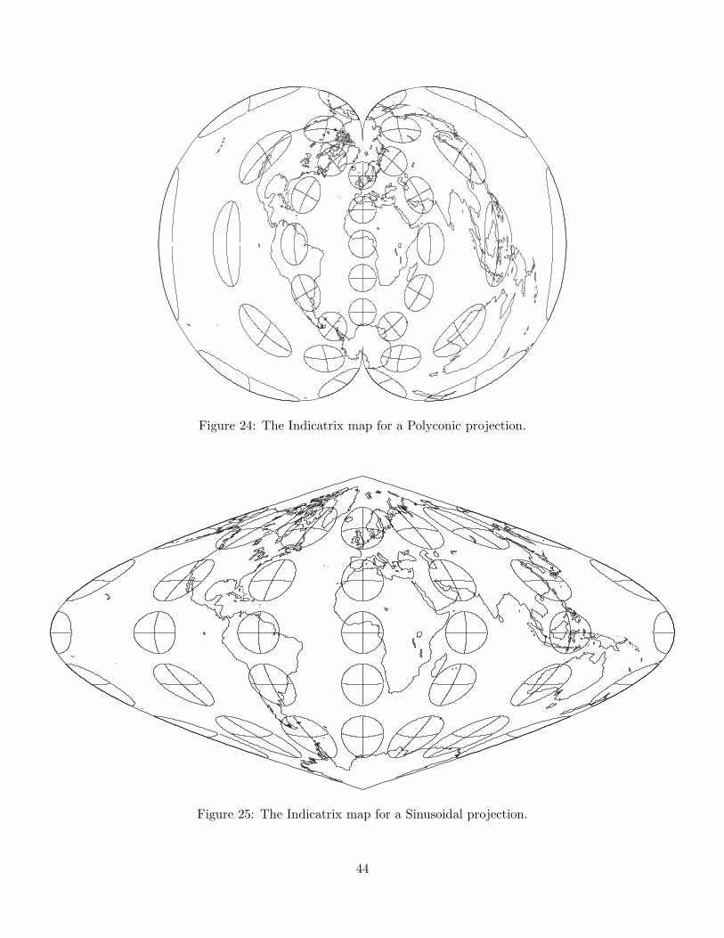
Figure 24: The Indicatrix map for a Polyconic projection.

Figure 25: The Indicatrix map for a Sinusoidal projection.

44

Figure 26: The Indicatrix map for a Winkel-Tripel projection.

Figure 27: The Indicatrix map for a Winkel-Tripel (Times Atlas) projection.

45