flexible pipe stress and fatigue analysis · 1 thesis work spring 2012 for stud. tech. henan li...
TRANSCRIPT
Flexible Pipe Stress and Fatigue Analysis
Henan Li
Marine Technology
Supervisor: Svein Sævik, IMT
Department of Marine Technology
Submission date: June 2012
Norwegian University of Science and Technology


1
THESIS WORK SPRING 2012
for
Stud. tech. Henan Li
Flexible Pipe Stress and Fatigue Analysis Spennings- og utmatnings-analyse av fleksible stigerør
The flexible riser represents a vital part of many oil and gas production systems.
During operation of such risers, several failure incidents may take place e.g. caused
by fatigue and corrosion. In limit cases where inspections indicate damage, the
decision making with regard to continue operation or replacing the riser may have
large economic and environmental consequences. Hence, the decision must be based
on accurate models to predict the residual strength of the pipe. In most applications,
one or several steel layers are used to carry the hoop stress resulting from internal
pressure. This is further combined with two layers of cross-wound armour tendons
(typically 40-60 tendons in one layer installed with an angle of 35o with the pipe’s
length axis) acting as the steel tensile armour to resist the tension and end cap wall
force resulting from pressure. The riser fatigue performance may in many cases be
governed by the dynamic stresses in the tensile armour. The existing lifetime models
for such structures is primarily based on inherent assumptions with respect to the slip
properties of the tensile armour. This thesis work focus on establishing a FEM based
model for analysis of the tensile armour, so as to analyse the stress and slip behaviour
when exposed to different load conditions. The thesis work is to be based on the
project work performed and shall include the following steps:
1) Literature study, including flexible pipe technology, failure modes and design
criteria, analytical methods for stress analysis of flexible pipes, non-linear
finite element methods relevant for non-linear FEM codes such as the Marintek
software Bflex2010. A detailed literature review on models for stress and slip
behaviour of flexible pipes shall be included and presented.
2) Establish four FE models in Bflex2010 using element type hshear353 with
associated contact and core elements: Assume one cross-section diameter
consisting of a two layered tensile armour with lay angles 25, 35, 45 and 55
degrees for each case.
3) From relevant literature, establish analytical formulas for stresses due to
axisymmetric loads and the stresses and slip due to bending.

2
4) Use the FE model to investigate the correlation between the numerical and
analytical stresses for the axisymmetric case as a function of internal pressure and
tension.
5) Use the FE model to study the motion and stresses of the armour tendon for
different levels of pre-stress, friction coefficient and bending curvature.
Compare with the analytical calculations.
6) Use the FE model to study cyclic effects with respect to the slip behaviour
assuming non-zero static curvature. Perform sensitivity with respect to the stick-
slip parameter and the two different assumption applied related to the layer
interaction in hcont453. Which of the two limit curves gives a best fit with regard
to the stress ranges between max and min curvature?
7) Conclusions and recommendations for further work
The work scope may prove to be larger than initially anticipated. Subject to approval
from the supervisors, topics may be deleted from the list above or reduced in extent.
In the thesis the candidate shall present his personal contribution to the resolution of
problems within the scope of the thesis work
Theories and conclusions should be based on mathematical derivations and/or logic
reasoning identifying the various steps in the deduction.
The candidate should utilise the existing possibilities for obtaining relevant literature.
Thesis format
The thesis should be organised in a rational manner to give a clear exposition of results,
assessments, and conclusions. The text should be brief and to the point, with a clear
language. Telegraphic language should be avoided.
The thesis shall contain the following elements: A text defining the scope, preface, list
of contents, summary, main body of thesis, conclusions with recommendations for
further work, list of symbols and acronyms, references and (optional) appendices. All
figures, tables and equations shall be numerated.
The supervisors may require that the candidate, in an early stage of the work, presents a
written plan for the completion of the work.
The original contribution of the candidate and material taken from other sources shall be
clearly defined. Work from other sources shall be properly referenced using an
acknowledged referencing system.
The report shall be submitted in two copies:
- Signed by the candidate

3
- The text defining the scope included
- In bound volume(s)
- Drawings and/or computer prints which cannot be bound should be organised in a
separate folder.
Ownership
NTNU has according to the present rules the ownership of the thesis. Any use of the thesis
has to be approved by NTNU (or external partner when this applies). The department has the
right to use the thesis as if the work was carried out by a NTNU employee, if nothing else
has been agreed in advance.
Thesis supervisors
Prof. Svein Sævik, NTNU.
Deadline: June 15th, 2012
Trondheim, January 15th, 2012
Svein Sævik
Candidate’s - date and signature:
Henan Li, January 15th, 2012
Flexible Pipe Stress and Fatigue Analysis
i
Table of content
ACKNOWLEDGEMENTS ........................................................................................ III
NOMENCLATURE ................................................................................................. IV
ABSTRACT .......................................................................................................... VII
LIST OF TABLES .................................................................................................. VIII
LIST OF FIGURES .................................................................................................. IX
CHAPTER1 INTRODUCTION ................................................................................... 1
1.1FLEXIBLE PIPE TECHNOLOGY ..........................................................................................1
1.2 SCOPE OF WORK ........................................................................................................9
CHAPTER2 ANALYTICAL DESCRIPTION FOR NONBONDED PIPES ........................... 11
2.1 INTRODUCTION .......................................................................................................11
2.2 MECHANICAL DESCRIPTION ........................................................................................11
2.3 ANALYTICAL DESCRIPTION FOR AXISYMMETRIC BEHAVIOUR ...............................................13
2.4 ANALYTICAL DESCRIPTION FOR BENDING .......................................................................22
2.5 FINITE ELEMENT IMPLEMENTATION .............................................................................25
CHAPTER3 NUMERICAL SOLUTIONS .................................................................... 27
3.1 INTRODUCTION .......................................................................................................27
3.2 BFLEX2010[8] .......................................................................................................27
3.3 FINITE ELEMENT MODELS IN BFLEX2010 ....................................................................27
CHAPTER4 NUMERICAL STUDIES ......................................................................... 34
4.1 INTRODUCTION .......................................................................................................34
4.2 COMPARISON ON NUMERICAL AND ANALYTICAL SOLUTIONS- AXISYMMETRIC LOADING ...........34
4.3 PARAMETER STUDY ON LOCAL DISPLACEMENTS UNDER BENDING .......................................44
4.4 COMPARISON ON NUMERICAL AND ANALYTICAL SOLUTIONS-BENDING ................................51
4.5 STUDY ON CYCLIC BENDING PROBLEM ..........................................................................73
CHAPTER 5 SUMMERY ........................................................................................ 84
5.1 CONCLUSIONS .........................................................................................................84
5.2 SUGGESTIONS FOR FUTURE WORK ...............................................................................85

Flexible Pipe Stress and Fatigue Analysis
ii
REFERENCE ......................................................................................................... 86
APPENDIX A ........................................................................................................... I
APPENDIX B .......................................................................................................... V

Flexible Pipe Stress and Fatigue Analysis
iii
Acknowledgements
This thesis has been carried out at Norwegian University of Science and Technology
(NTNU), Department of Marine Technology under the supervision of Professor.
Svein Sævik. His suggestion and instructions are gratefully acknowledged.
Sincere thanks also give to the Senior Scientist Naiquan Ye at MARINTEK. His
patient assistance on both analytical and software study helps me perform better of
the thesis.
Thanks are also given to my classmates at Marine Technology who give helpful
discussion throughout the thesis study.

Flexible Pipe Stress and Fatigue Analysis
iv
Nomenclature
Symbols Explanation
b Thickness of tendon cross section(mm).
Yong’s modulus of elasticity (N ).
Shear modulus(N ).
Penalty stiffness parameter.
G Determinant of metric tensor.
Base vectors directed along the local curvilinear coordinate in
undeformed configurations.
Base vectors directed along curve principal torsion-flexure axes.
Cross section torsion constant ( ).
Inertia moment about axis ( ).
Distributed moment acting about the local coordinate axes (N).
Moment stress resultant acting about the local coordinate axes (Nm).
Force stress resultants acting along the local coordinate axes (N).
Distributed loads acting along the local coordinate axes (N ).
Distributed tangential reaction.
Radius from pipe centre line to tendon centre line (m).
Surface of rod in undeformed, deformed configurations.

Flexible Pipe Stress and Fatigue Analysis
v
Vector and component form of displacement field.
Surface coordinates.
Internal virtual work contribution from beam element.
Local curvilinear coordinates.
Cartesian coordinates refers to a Cartesian coordinate system
arbitrarily positioned along the pipe centre line.
Tendon lay angle.
Global pipe axial strain.
Axial strain of rod.
Rotation about the local curvilinear axis.
Principal curvature along curve ( ).
Total accumulated torsion of tendon centre line ( ).
Total accumulated transverse curvature of the tendon centre line
( ).
Total accumulated normal curvature of tendon centre line ( ).
Principal curvatures of the supporting surface ( ).
Pipe surface curvature in transverse tendon direction (along the
axis) ( ).
Curvature radius of pipe surface at neutral axis (m).
Tensor and component form of the Cauchy stress tensor in the local
Cartesian coordinate system.

Flexible Pipe Stress and Fatigue Analysis
vi
Torsion along curve ( ).
ϕ Spherical coordinate angle
ω Angle between surface normal and curve normal.
ω Torsion deformation, i.e., twist ( ).
ω Transverse curvature deformation ( ).
ω Normal curvature deformation ( ).
Relative displacement vector or component.
Components of beam rotation.
Incremental potential

Flexible Pipe Stress and Fatigue Analysis
vii
Abstract
Fatigue is an important character for the flexible pipes as they are always exposed to
dynamic loading. For nonbonded flexible pipes, fatigue and stress analysis can be
performed based on different assumptions of slip behaviour. Different slip
assumptions used in estimating the slip stress always play a determinative role in the
prediction of fatigue damage. Thus, this thesis will focus on the study of the slip
behaviour between tensile armour layers of nonbonded flexible pipes. The results can
be used to support the basic assumptions for further fatigue analysis.
The main object of this thesis is to summarize the existing analytical methods for
stress and slip analysis of nonbonded flexible pipe armouring layers and to verify that
the improved finite element models can give adequate description of the flexible pipe
slip behaviour.
In previous version of BFLEX, the transverse slip effect for nonbonded flexible pipes
has been neglected. In this thesis, transverse slip regime has been activated in the
updated BFLEX by developing a new type of beam element hshear353 and a new
type of contact element hcont453. Finite element models use these two elements have
been made and several case studies have been carried out.
For axisymmetric loading, two analytical solutions, one obtained from the equations
by Witz&Tan[13]
, one from Sævik[2]
have been compared with the result from
numerical simulation. It has been found that Sævik’s solution matches better with the
BFLEX solution comparing to Witz&Tan’s solution.
For flexible pipes exposed to bending, influences on slip behaviour from several pipe
parameters, namely friction coefficient, axial strain and global pipe curvature, have
been investigated. The numerical results are also compared with analytical solutions
obtained from Sævik[2]
. It has been found that the numerical solutions can give
excellent agreement with analytical solutions. It is further concluded that the outer
tensile armour layer do not influence much on the inner layer slip behaviour.
In addition, the cyclic bending effects on nonbonded flexible pipes have been
investigated. It has been found that the tendon behaves differently from case to case.
The inner and outer layers behave differently. Only a few cases have been studied for
this problem due to time limitation.
The overall conclusion is that the developed BFLEX model is capable of describing
the stresses and local displacements of flexible pipe for simple cases. The developed
numerical model can further be used in the study of fatigue in flexible risers.
However, more studies on influence from multi-tensile layers and cyclic bending are
needed in the future.

Flexible Pipe Stress and Fatigue Analysis
viii
List of tables
Table 1-1 Global failure modes[4]
.................................................................................. 7
Table 1-2 Design criteria for pressure and tensile armours[4]
........................................ 9
Table 3-1 Finite element modeling properties for the simplified model ..................... 28
Table 3-2 Finite element modeling properties for the model with two armour layers 29
Flexible Pipe Stress and Fatigue Analysis
ix
List of figures
Figure 1-1 Flexible riser configurations[2]
..................................................................................... 2
Figure 1-2 Flexible pipe cross section [4]
....................................................................................... 4
Figure 1-3 typical profile of the carcass[4]
..................................................................................... 5
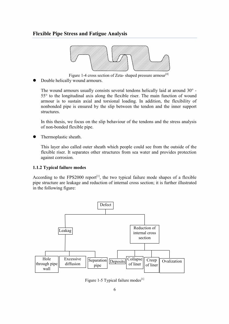
Figure 1-4 cross section of Zeta- shaped pressure armour[4]
......................................................... 6
Figure 1-5 Typical failure modes[1]
............................................................................................... 6
Figure 2-1 Models for cross-sectional analysis[5]
........................................................................ 11
Figure 2-2 Axisymmetric loading behaviour[2]
........................................................................... 12
Figure 2-3 Bending behaviour[2]
.................................................................................................. 12
Figure 2-4 Definition of pipe center line system and basic quantities[2]
..................................... 14
Figure 2-5 The system[2]
....................................................................................................... 14
Figure 2-6 system relative orientation to system[2]
........................................................ 16
Figure 2-7 Restraint of the curvilinear plane[2]
............................................................................ 17
Figure 2-8 Curved infinitesimal beam element[2]
........................................................................ 18
Figure 2-9 Geometric relation[2]
.................................................................................................. 20
Figure 2-10 Components of deformation in local system[2]
........................................................ 21
Figure 2-11 a. Slip from compression side to the tensile side[5]
b. The two limited curves[14]
. 23
Figure 2-12 Eight (Ten) DOFs curved infinitesimal beam element[2]
......................................... 26
Figure 2-13 Coordinate system in BFLEX 2010[8]
...................................................................... 26
Figure 3-1 Simplified BFLEX model, single tendon .................................................................. 28
Figure 3-2 Complex BFLEX model, double tensile armour layers............................................. 29
Figure 3-3 coordinate system for hshear353[10]
........................................................................... 31
Figure 3-4 New contact element hcont453[9]
............................................................................... 33
Figure 4-1 Curvature increments as a function of axial strain- 25°lay angle .............................. 36
Figure 4-2 Curvature increments as a function of axial strain-35°lay angle ............................... 37
Figure 4-3 Curvature increments as a function of axial strain-45°lay angle ............................... 38
Figure 4-4 Curvature increments as a function of axial strain-55°lay angle ............................... 38
Figure 4-5 Curvature increments as a function of torsion-25°lay angle ..................................... 39
Figure 4-6 Curvature increments as a function of torsion-35°lay angle ..................................... 40
Figure 4-7 Curvature increments as a function of torsion-45°lay angle ..................................... 40
Figure 4-8 Curvature increments as a function of torsion-55°lay angle ..................................... 41
Figure 4-9 Curvature increments as a function of radial displacement-25°lay angle ................. 42
Figure 4-10 Curvature increments as a function of radial displacement-35°lay angle ............... 42

Flexible Pipe Stress and Fatigue Analysis
x
Figure 4-11 Curvature increments as a function of radial displacement-45°lay angle ............... 43
Figure 4-12 Curvature increments as a function of radial displacement-55°lay angle ............... 43
Figure 4-13 Maximum longitudinal displacement as a function of global pipe curvature .......... 45
Figure 4-14 Maximum transverse displacement as a function of global pipe curvature ............. 45
Figure 4-15 Maximum twist curvature increment as a function of global pipe curvature .......... 45
Figure 4-16 Maximum transverse curvature increment as a function of global pipe curvature .. 46
Figure 4-17 Maximum normal curvature increment as a function of global pipe curvature ....... 46
Figure 4-18 Maximum longitudinal displacement as a function of friction coefficient .............. 47
Figure 4-19 Maximum transverse displacement as a function of friction coefficient ................. 47
Figure 4-20 Maximum twist curvature increment as a function of friction coefficient .............. 48
Figure 4-21 Maximum transverse curvature increment as a function of friction coefficient ...... 48
Figure 4-22 Maximum normal curvature increment as a function of friction coefficient ........... 48
Figure 4-23 Maximum longitudinal displacement as a function of axial strain .......................... 49
Figure 4-24 Maximum transverse displacement as a function of axial strain ............................. 49
Figure 4-25 Maximum twist curvature increment as a function of axial strain .......................... 50
Figure 4-26 Maximum transverse curvature increment as a function of axial strain .................. 50
Figure 4-27 Maximum normal curvature increment as a function of axial strain ....................... 50
Figure 4-28 Longitudinal slip- 25°lay angle ............................................................................... 52
Figure 4-29 Longitudinal slip- 35°lay angle ............................................................................... 52
Figure 4-30 Longitudinal slip- 45°lay angle ............................................................................... 53
Figure 4-31 Longitudinal slip- 55°lay angle ............................................................................... 53
Figure 4-32 Maximum longitudinal slip as a function of lay angle ............................................ 54
Figure 4-33 Transverse slip- 25°lay angle .................................................................................. 55
Figure 4-34 Transverse slip- 35°lay angle .................................................................................. 55
Figure 4-35 Transverse slip- 45°lay angle .................................................................................. 56
Figure 4-36 Transverse slip- 55°lay angle .................................................................................. 56
Figure 4-37 Maximum transverse slip as a function of lay angle ............................................... 57
Figure 4-38 Twist curvature increment- 25°lay angle ................................................................. 58
Figure 4-39 Twist curvature increment- 35°lay angle ................................................................. 59
Figure 4-40 Twist curvature increment- 45°lay angle ................................................................. 59
Figure 4-41 Twist curvature increment- 55°lay angle ................................................................. 60
Figure 4-42 Maximum twist curvature increment as a function of lay angle ............................. 60
Figure 4-43 Modified twist curvature increment-25°lay angle ................................................... 62
Figure 4-44 Modified twist curvature increment- 35°lay angle .................................................. 62

Flexible Pipe Stress and Fatigue Analysis
xi
Figure 4-45 Modified twist curvature increment- 45°lay angle .................................................. 63
Figure 4-46 Modified twist curvature increment- 55°lay angle .................................................. 63
Figure 4-47 Maximum twist curvature change with longitudinal slip, modified ........................ 64
Figure 4-48 Transverse curvature increment- 25°lay angle ........................................................ 65
Figure 4-49 Transverse curvature increment- 35°lay angle ........................................................ 65
Figure 4-50 Transverse curvature increment- 45°lay angle ........................................................ 66
Figure 4-51 Transverse curvature increment- 55°lay angle ........................................................ 66
Figure 4-52 Maximum transverse curvature increment as a function of lay angle ..................... 67
Figure 4-53 Normal curvature increment- 25°lay angle ............................................................. 68
Figure 4-54 Normal curvature increment- 35°lay angle ............................................................. 68
Figure 4-55 Normal curvature increment- 45°lay angle ............................................................. 69
Figure 4-56 Normal curvature increment- 55°lay angle ............................................................. 69
Figure 4-57 Modified normal increment- 25°lay angle............................................................... 70
Figure 4-58 Modified normal increment- 35°lay angle............................................................... 71
Figure 4-59 Modified normal curvature increment- 45°lay angle............................................... 71
Figure 4-60 Modified normal curvature increment- 55°lay angle............................................... 72
Figure 4-61 Maximum normal curvature increment as a function of lay angle, modified .......... 73
Figure 4-62 Twist curvature as a function of time, axial strain’s influence ................................ 74
Figure 4-63 Normal curvature as a function of time, axial strain’s influence ............................. 75
Figure 4-64 Twist curvature as a function of time, axial strain’s influence, modified ............... 76
Figure 4-65 Normal curvature as a function of time, axial strain’s influence, modified ............ 76
Figure 4-66 Twist curvature as a function of time, friction’s influence ...................................... 77
Figure 4-67 Normal curvature as a function of time, friction’s influence ................................... 77
Figure 4-68 Twist curvature as a function of time, friction’s influence ...................................... 78
Figure 4-69 Normal curvature as a function of time, friction’s influence ................................... 79
Figure 4-70 Twist curvature as a function of time, friction’s influence, modified ..................... 79
Figure 4-71 Normal curvature as a function of time, friction’s influence, modified .................. 80
Figure 4-72 Twist curvature as a function of time, inner layer ................................................... 81
Figure 4-73 Normal curvature as a function of time, inner layer ................................................ 81
Figure 4-74 Twist curvature as a function of time, outer layer ................................................... 82
Figure 4-75 Normal curvature as a function of time, outer layer ................................................ 82

Flexible Pipe Stress and Fatigue Analysis
1
Chapter1 Introduction
1.1Flexible pipe technology
Flexible pipes are widely used in offshore oil and gas industry as connections for both
fixed and floating platforms. Examples are risers connecting seabed to the surface and
well product flowlines. The presence of flexible pipe offers the permanent connection
between floating structures and subsea installations under extreme dynamic conditions
because it can suffer larger bending deformations. At the same time, it is easy to
transport and install. The most important characters for flexible pipe are lower bending
stiffness and higher volume stiffness.
1.1.1 Applications
Common applications for flexible pipes are listed below[1]
:
Riser used to connect subsea installations with above water production facilities
during the production phase.
Flowlines for in-field connection of wellheads, templates, loading terminals, etc.
Jumper lines between fixed and floating platforms.
Loading hoses for offshore loading terminals.
Small-diameter service lines, such as kill and choke lines, umbilicals, etc.
The present thesis will only focus on the response of flexible pipes used in fully
dynamic riser systems connecting offshore production and offshore systems. Thus, only
details on riser systems are discussed.
Key parameters for a riser system are the number, sizes, pressure, rating and internal
coating requirements related to transfer function
According to [1], the requirements for the riser system support depend on
Water depth
Support vessel motions
Current and wave loading
Key parameters for external loadings are:
Tension
Curvature
Flexible Pipe Stress and Fatigue Analysis
2
Torsion
Contact with other structures(interference)
Compression
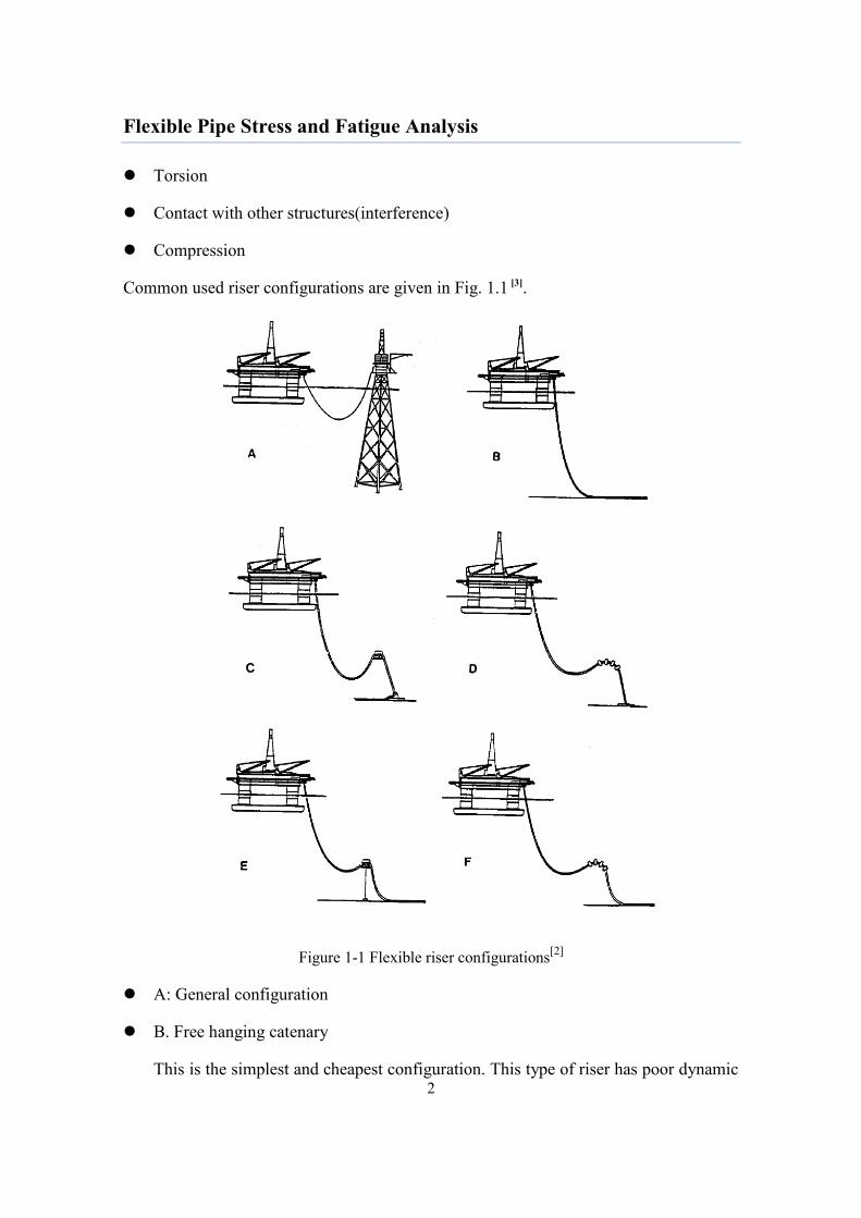
Common used riser configurations are given in Fig. 1.1 [3].
Figure 1-1 Flexible riser configurations[2]
A: General configuration
B. Free hanging catenary
This is the simplest and cheapest configuration. This type of riser has poor dynamic

Flexible Pipe Stress and Fatigue Analysis
3
properties and severe response at the touch down area where the riser is connected
to the vessel. It is reported that this type of configuration is likely to have
compression buckling under large vessel motions[3] and large top tension when
applied in deep water.
C: Steep S
For this shape of pipe, a buoy, either fixed or floating, is used to connect to the pipe
to create the S-shape. The buoy can absorb the tension variation from the platform,
and such the touch down point (TDP) has only small variation in tension. The S
configuration is costly and only used for complex installation procedure. The steep
S has larger curvature than lazy S.
D: Steep wave
In this configuration, buoyancy elements which is made by synthetic foam, is
mounted on a longer length of the riser. A negative submerged weight is created by
the buoyancy elements and a wave shape is made. This will decouple the vessel
motion from the TDP. The steep wave configuration also needs a subsea base and a
subsea bending stiffener. This type of configuration is commonly used in cases
where the internal fluid density changes during life time. One problem of wave
configuration is the buoyance elements tend to lose volume under high pressure and
thus results an increased submerged weight. The wave configuration has to be
designed to have up to 10% loss of buoyancy.
E: Lazy S
Lazy S configuration is similar with steep S configuration but with smaller
curvature.
F: Lazy wave
The lazy wave configuration has similar principle as for steep wave configuration
but with smaller curvature. The main difference is that the lazy wave does not
require a subsea base and bend stiffener. Lazy wave is lower cost and more often
preferred.
1.1.2 Classification on cross section properties[4]
Flexible pipe can be divided into bonded and nonbonded pipes based on cross section
properties, i.e., the different principles of providing flexibility.
Layers for nonbonded flexible pipe are not fixed and free to move against each other.
The flexibility of nonbonded pipe is provided by the relative slip of armouring tendons.
Nonbonded pipes are often used as risers and be constructed in length up to several
kilometers.

Flexible Pipe Stress and Fatigue Analysis
4
The relative slip is not available for bonded pipe since its layers are bonded with each
other. The principle for bonded pipe is that the rubber has a relatively low shear
modulus which will control and restrict the stresses induced by bending and hence
provide flexibility. Bonded flexible pipe is mostly used when short length is required,
due to the limitation of length per segment.
Typical cross sections for bonded and nonbonded pipe are given in the figure below[4].
Figure 1-2 Flexible pipe cross section [4]

Flexible Pipe Stress and Fatigue Analysis
5
Namely:
1. Tensile layer
2. Anti-friction layer
3. Outer sheath
4. Hoop stress layer
5. Outer layer of tensile armour
6. Anti-wear layer
7. Inner layer of tensile armour
8. Back-up pressure armour
9. Interlocked pressure armour
10. Internal pressure sheath
11. Carcass
12. Anti-bird-cage layer
1.1.3 Cross section properties for nonbonded pipes
Today’s dominating type of flexible pipe is the nonbonded pipe, which will be the main
focus of this thesis work. A brief function description of main layers for nonbonded
pipe is given below:
Carcass
Carcass is often the innermost layer of the nonbonded pipe. The function of inter
locked stainless steel carcass is to provide resistance to the external hydrodynamic
pressure and prevent collapse of the internal pressure sheath. Since the carcass will
contact the inner fluid directly, its material is chosen due to anti-corrosion
consideration. It is made of a stainless steel flat strip that is formed into an
interlocking profile, which is shown in figure 1-3.
Figure 1-3 typical profile of the carcass[4]
Internal pressure sheath
Internal pressure sheath is used as sealing component provides internal fluid
integrity. Usually, it is made from a thermoplastic by extrusion over the carcass.
Pressure armour (Zeta spiral for example)
Pressure armour consists of an interlocking profile, typically like the Zeta profile
shown in the figure below, but other designs are known in use. Zeta spiral is made
of Z-shaped interlocking wires. The pressure armour is used to provide capacity of
loading in hoop direction caused by internal and external pressure. The pressure
armour is typical made of low-alloyed carbon steel grades, with typical high yield
strength.
Flexible Pipe Stress and Fatigue Analysis
6
Figure 1-4 cross section of Zeta- shaped pressure armour
[4]
Double helically wound armours.
The wound armours usually consists several tendons helically laid at around 30° -
55° to the longitudinal axis along the flexible riser. The main function of wound
armour is to sustain axial and torsional loading. In addition, the flexibility of
nonbonded pipe is ensured by the slip between the tendon and the inner support
structures.
In this thesis, we focus on the slip behaviour of the tendons and the stress analysis
of non-bonded flexible pipe.
Thermoplastic sheath.
This layer also called outer sheath which people could see from the outside of the
flexible riser. It separates other structures from sea water and provides protection
against corrosion.
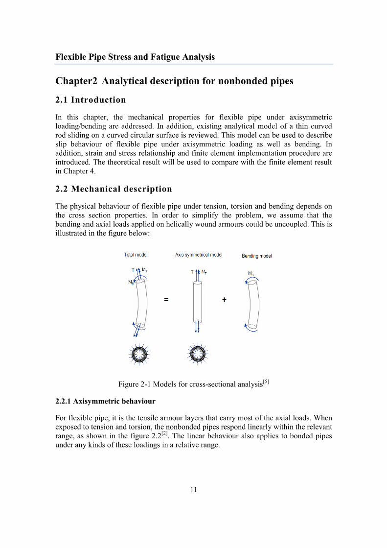
1.1.2 Typical failure modes
According to the FPS2000 report[1], the two typical failure mode shapes of a flexible
pipe structure are leakage and reduction of internal cross section; it is further illustrated
in the following figure:
Figure 1-5 Typical failure modes[1]
Hole
through pipe
wall
Excessive
diffusion Separation
pipe Ovalization
Collapse
of liner Deposits Creep
of liner
Defect
Reduction of
internal cross
section
Leakag
e

Flexible Pipe Stress and Fatigue Analysis
7
One commonly used standard to design failure modes is American Petroleum Institute
(API) standard 17B[4].
Since this thesis will mainly focus on the behaviour of non-bonded pipe armours , only
the related failure modes are introduced. Details regarding other failure modes, please
refer to API, ‘Recommended Practice for Flexible Pipe 17B’.
Failures in armours can be caused by over load tension, compression, bending, torsion
as well as fatigue. Also, the erosion of armour because of contacting sea water or
diffused fluid should be taken into account if applicable. A short summery of API
standard 17B[4] regarding failure mode of armours is given in the table below.
Table 1-1 Global failure modes[4]
Pipe global
failure mode to
design against
Potential failure mechanisms
caused by armours
Design solution or
variables
Tensile failure Rupture of tensile armours due to
excess tension
1)Increase tendon
thickness or select higher
strength material if
feasible
2)Modity comfiguration
designs to reduce loads
3)Add two more armour
layers
4)Bury pipe
Compressive
failure
Bird-caging of tensile-armour
tendons
1)Avoid riser
configurations that cause
excessive pipe
compression
2)Provide additional
support/restraint for
tensile armours, such as
tape and/additional or
thicker outer sheath
Overbending Collapse of pressure armour Modify configuration
designs to reduce loads

Flexible Pipe Stress and Fatigue Analysis
8
Torsional failure 1)Failure of tensile armour
tendon
2)Bird-caging of tensile-armour
wires
1)Modify material
selection
2)Modify cross-section
design(e.g. change lay
angle of tendons, add extra
layer outside armour
tendons, ets.) to increase
torsional capacity
Fatigue failure 1)Tensile-armour-tendon fatigue
2)Pressure-armour-tendon fatigue
1)Increase tendon
thickness or select
alternative material, so
that fatigue streeses are
compatible with service-
life requirements.
2)Modify design to reduce
fatigue loads.
1.1.3 Design criteria
This chapter is based on the design criterion given by the API standard: Recommended
Practice for Flexible Pipe 17B[4]
.
The design criteria for flexible pipes can generally be given in terms of the following
design parameters:
Strain (polymer sheath, unbonded pipe)
Creep (internal pressure sheath, unbonded pipe)
Stress (metallic layers and end fitting)
Hydrostatic collapse (buckling load)
Mechanical collapse(stress introduced from armour layers)
Torsion
Crushing collapse and ovalization (during installation)
Compression (axial and effective)
Service-life factor

Flexible Pipe Stress and Fatigue Analysis
9
In this thesis, we focus on the design criteria regarding armours. The degradation modes
of the pressure and tensile armours include corrosion, disorganization or locking of
armouring wires as well as fatigue and wear. The recommended criteria concluded from
API 17B[4] is showed in the following table.
Table 1-2 Design criteria for pressure and tensile armours[4]
Component Degradation mode Design solution or
variables
Pressure and tensile
armours
Corrosion Only general corrosion
accepted, no crack
initiation acceptable.
Disorganization or locking
of armouring wires
No disorganization of
armouring wires when
bending to minimum bend
radius.
Fatigue and wear It is necessary to give
consideration in the design
of flexible pipe to service
life or replacement of
components/ancillary
equipment as part of an
overall service-life policy.
Details in chapter 8.2.4
1.2 Scope of work
As mentioned above, this thesis will focus on the stress analysis and the slip behaviour
of nonbonded flexible pipe.
Existing research on nonbonded flexible pipe states: when friction force is taken into
account, the slip in transverse direction will become very small. Thus, in some software,
e.g. previous BFLEX2010, transverse slip has been neglected in order to reduce the
number of degrees of freedom.
In this thesis, the modified version of BFLEX2010 with a new beam element hshear353
and a new contact element hcont453 which can be used to describe transverse slip
behaviour are used. Two BFLEX models with different pipe parameters are studied and
compared to the analytical solution.

Flexible Pipe Stress and Fatigue Analysis
10
In chapter 2, existing analytical model valid for thin curved rods sliding on a curved
circular surface are studied. Both axisymmetric and bending behaviour are discussed.
Finite element implementation procedure is described.
In chapter 3, an introduction of BFLEX2010 is given. The finite element models used in
this thesis together with formulations of the new element types are described.
In chapter 4, numerical simulations using the bflex models introduced in Chapter 3 are
carried out.The numerical results are compared with analytical solutions in order to
verify whether the modified BFLEX version can provide enough accuracy when
describing the tendon’s kinematic. Cases regarding to multi-layer influence and cyclic
bending effects on local stress and slip behaviour are also carried out.
In chapter 5, a summary of the thesis and suggestions for future work are given.
Flexible Pipe Stress and Fatigue Analysis
11
Chapter2 Analytical description for nonbonded pipes
2.1 Introduction
In this chapter, the mechanical properties for flexible pipe under axisymmetric
loading/bending are addressed. In addition, existing analytical model of a thin curved
rod sliding on a curved circular surface is reviewed. This model can be used to describe
slip behaviour of flexible pipe under axisymmetric loading as well as bending. In
addition, strain and stress relationship and finite element implementation procedure are
introduced. The theoretical result will be used to compare with the finite element result
in Chapter 4.
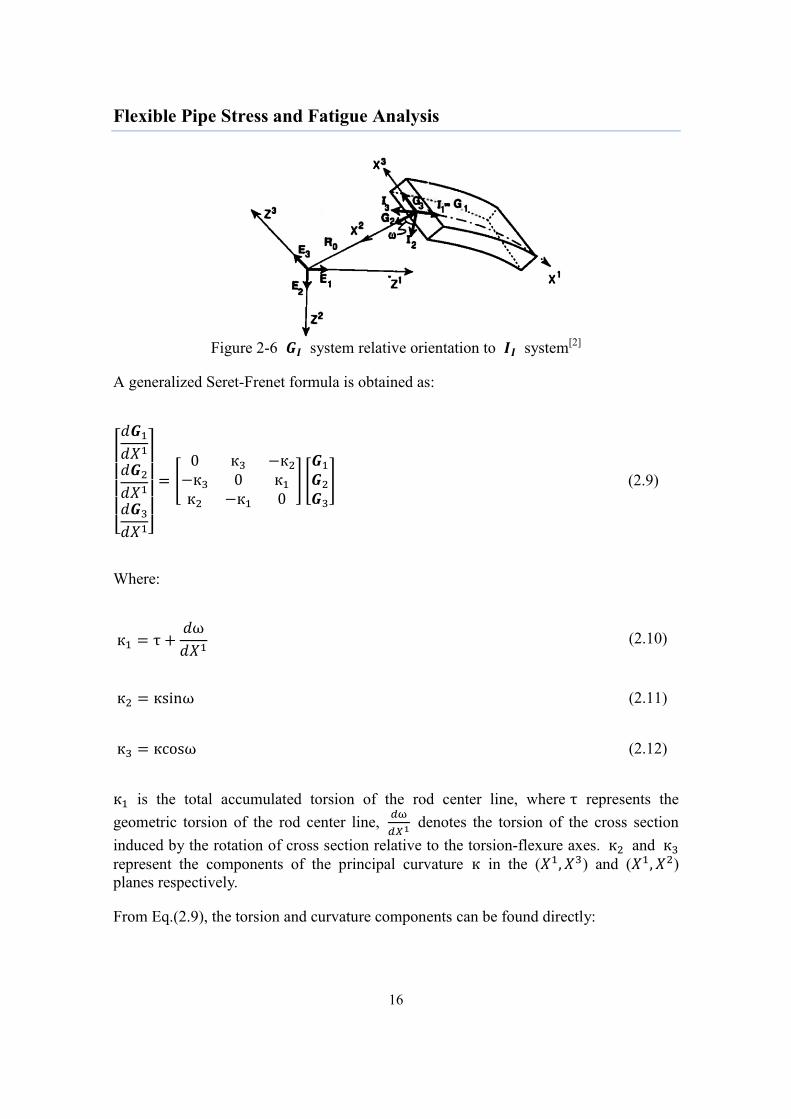
2.2 Mechanical description
The physical behaviour of flexible pipe under tension, torsion and bending depends on
the cross section properties. In order to simplify the problem, we assume that the
bending and axial loads applied on helically wound armours could be uncoupled. This is
illustrated in the figure below:
Figure 2-1 Models for cross-sectional analysis[5]
2.2.1 Axisymmetric behaviour
For flexible pipe, it is the tensile armour layers that carry most of the axial loads. When
exposed to tension and torsion, the nonbonded pipes respond linearly within the relevant
range, as shown in the figure 2.2[2]
. The linear behaviour also applies to bonded pipes
under any kinds of these loadings in a relative range.

Flexible Pipe Stress and Fatigue Analysis
12
A
Figure 2-2 Axisymmetric loading behaviour[2]
2.2.2 Bending behaviour
Bending is one of the most important properties of flexible pipe comparing to ordinary
steel risers. For a nonbonded pipe, this property is ensured by the slip between the
armour tendons and the supporting structure. The nonbonded flexible pipe has a non-
linear moment-curvature relationship as illustrated in the figure below.
Figure 2-3 Bending behaviour[2]
It can be divided into three steps:
Step1, Ordinary beam- bending phase, small curvature
In this step, the cross-section of the tendon remains plane. This shows that no slip exists
between tendon and supporting structure. The pipe will bend with a similar stiffness as a
steel pipe with same cross section.

Flexible Pipe Stress and Fatigue Analysis
13
Step2, Low bending stiffness phase, intermedium curvature
As the moment applied on flexible pipe increases, slip will occur when the bending
moment overcomes friction moment of the pipe, due to the development of shear stress
in armour layer and the supporting structure. The bending stiffness in this step drops
significantly. We define the bending stiffness at this step ‘sliding bending stiffness’ and
it is govern by the stiffness of the plastic tubules and strain energy in each armour
tendon.
Step3, Increasing bending stiffness, critical curvature
This phase begins at when the gap between each tendon is closed. In this phase, no
sliding is allowed anymore. This is termed as critical radius and should be avoid in any
operation.
In the following, this thesis pays its attention to step2 when studying the slip behaviour
under bending. Basic assumptions are[4]
:
1, The bending stiffness induced by local tendon behaviour at end restraints is at least
one order of magnitude less than the effect of the total cross section bending stiffness
and hence can be neglected. This is considered to be a reasonable assumption along the
bending stiffener.
2, Each tendon behaves independently for the curvature range considered. This
assumption is considered reasonable as long as the curvature is smaller than the critical
curvature.
2.3 Analytical description for axisymmetric behaviour
In this part, an existing analytical model of a tube layer with an individual tendon
sliding on it is reviewed. The model can be used to describe the armour tendon’s
behaviour under either axisymmetric loading or bending. Axisymmetric behaviour is
discussed in this sub-chapter, and bending behaviour will be discussed in Chapter 2.4.
Since axisymmetric loading, i.e., tension, torsion and pressure does not change the
shape of the pipe cross section. Therefore, axisymmetric behaviour can be assumed and
relatively simple relations can be obtained.
2.3.1 Coordinate system
In order to describe a point on the surface of a circular cylinder with a constant radius
, a fixed Cartesian coordinate system with axes ZI and unit vectors EI is used.
Supporting surface is represented by the radius R and surface coordinates w and v. See
figure below.

Flexible Pipe Stress and Fatigue Analysis
14
Figure 2-4 Definition of pipe center line system and basic quantities[2]
The Cartesian coordinates of an arbitrary point on the circular surface is hence
expressed by Eq.(2.1)-(2.3):
( ) (2.1)
( ) (2.2)
(2.3)
When the pipe is exposed to high tensile stress, it is reasonable to assume that the rod
cross section principal axes are fixed to the surface normal. In addition, a local
orthonormal axes constructed at an arbitrary point with unit base vector is developed
in order to describe the principal torsion-flexure axes along the curve. See figure 2-5.
Figure 2-5 The system
[2]
The rotation of the local unit triad along an infinitesimal distance is given by the Seret-
Frenet[6]
differential formula, where represents for the arc length coordinate:

Flexible Pipe Stress and Fatigue Analysis
15
[ 𝑑 𝑑
𝑑 𝑑
𝑑 𝑑 ]
[0 к 0 к 0 𝜏0 𝜏 0
] [
] (2.4)
Then, the torsion and principal curvature к can be determined directly:
∙𝑑 𝑑
(2.5)
к ∙𝑑 𝑑
(2.6)
Which for a rod being wound onto a circular helix gives:
(2.7)
к
(2.8)
In addition, base vectors directed along the local curvilinear coordinate axes is
introduced. is directed parallel to , is oriented along the inwards surface
normal and fixed to the cross section principal axes, is defined by the orthonormality
condition. The angle between and is defined as ω, which represents for the
relative rotation from cross section principal axes to the torsion-flexure axes as shown
in the figure below.
Flexible Pipe Stress and Fatigue Analysis
16
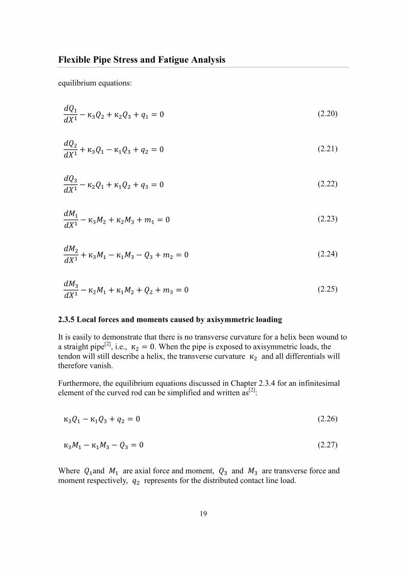
Figure 2-6 system relative orientation to system
[2]
A generalized Seret-Frenet formula is obtained as:
[ 𝑑
𝑑
𝑑
𝑑
𝑑
𝑑 ]
[0 к к
к 0 к к к 0
] [
] (2.9)
Where:
к +𝑑ω
𝑑 (2.10)
к к ω (2.11)
к к ω (2.12)
к is the total accumulated torsion of the rod center line, where represents the
geometric torsion of the rod center line, 𝑑ω
𝑑𝑋1 denotes the torsion of the cross section
induced by the rotation of cross section relative to the torsion-flexure axes. к and к
represent the components of the principal curvature к in the ( ) and ( )
planes respectively.
From Eq.(2.9), the torsion and curvature components can be found directly:

Flexible Pipe Stress and Fatigue Analysis
17
к ∙𝑑
𝑑 (2.13)
к ∙𝑑
𝑑 (2.14)
к ∙𝑑
𝑑 (2.15)
The transverse curvature will only occur when ω differs from zero, i.e., the surface
normal dose not coincide with curve normal. Eq. (2.13)-(2.15) are used to find out the
curvature increments in sub chapter 2.4.2.
2.3.3 Kinematic restraint
It is assumed that the tendon is forced to slide along the curvilinear axes and
only, thus the full three dimensional description can be eliminated.
Figure 2-7 Restraint of the curvilinear plane
[2]
Thus, a restraint on the rotation of the rod about the axis is introduced:
к + к (2.16)
Where and represent for the tendon’s longitudinal and transverse displacement
along the local curvilinear axes respectively.

Flexible Pipe Stress and Fatigue Analysis
18
к is the pipe surface transverse curvature along direction and could be expressed
by the following equation:
Similarly,
к к + к (2.17)
Where к and к represent the principal curvatures in the circumferential and
longitudinal directions of the surface, where
к
(2.18)
к
(2.19)
2.3.4 Equilibrium equation
Figure 2-8 shows the forces and moments on an infinitesimal element of the curved rod.
Figure 2-8 Curved infinitesimal beam element[2]
At the first end, there is a local coordinate system with axes and base vector
together with stress resultants 𝑸 and 𝑴 . The axes are fixed to the rod cross section
principal axes. At the second end, the axes change to + 𝑑 and the stress change to
𝑸 + 𝑑𝑸 and 𝑴 + 𝑑𝑴 . Consider force and moment equilibrium and introduce the
generalized Seret-Frenet formula from Eq.(2.9), we can obtain the following six coupled
Flexible Pipe Stress and Fatigue Analysis
19
equilibrium equations:
𝑑
𝑑 к + к + 0 (2.20)
𝑑
𝑑 + к к + 0 (2.21)
𝑑
𝑑 к + к + 0 (2.22)
𝑑
𝑑 к + к + 0 (2.23)
𝑑
𝑑 + к к + 0 (2.24)
𝑑
𝑑 к + к + + 0 (2.25)
2.3.5 Local forces and moments caused by axisymmetric loading
It is easily to demonstrate that there is no transverse curvature for a helix been wound to
a straight pipe[2]
, i.e., к 0. When the pipe is exposed to axisymmetric loads, the
tendon will still describe a helix, the transverse curvature к and all differentials will
therefore vanish.
Furthermore, the equilibrium equations discussed in Chapter 2.3.4 for an infinitesimal
element of the curved rod can be simplified and written as[2]
:
к к + 0 (2.26)
к к 0 (2.27)
Where and are axial force and moment, and are transverse force and
moment respectively, represents for the distributed contact line load.

Flexible Pipe Stress and Fatigue Analysis
20
Eq. (2.26) represents the force equilibrium equation in the radial direction, Eq.(2.27)
represents the moment equilibrium equation about the surface normal. When knowing
the expression of in terms of twist and curvature induced by axisymmetric
loading, the unknown contact pressure and shear force can be eliminated. In
this part, analytical solution from Sævik.S[2]
considering all the terms discussed above is
introduced.
Axial force
The axial force can be found by using the axial strain of the tendon centre line
as a function of pipe global axial strain, local radial displacements and global twist
given as:
+ 𝜃 (2.28)
Where is the global axial strain caused by tension; is the radial displacement of
the pipe induced by pressure; 𝜃 is the global twist which represents torque. They are
defined in the figure below:
Figure 2-9 Geometric relation
[2]
The axial force is found by:
𝐴 (2.29)
Where is the Young’s modulus of elasticity (N ), 𝐴 is the rod cross section area
( ).
Moments

Flexible Pipe Stress and Fatigue Analysis
21
The twist and normal curvature increments can be calculated by moving the rod from
stress free state to the deformed equilibrium state. By using the coordinate system
introduced in Chapter 2.3.1, it is found:
к к + (к к ) + к к (2.30)
к к (к ) + к (2.31)
and represent the twist and normal curvature increments. and are
the derivatives of and .
By decomposing the global displacements along the local coordinate axes shown in
figure 2-10, the displacement differentials are obtained:
+ 𝜃 (2.32)
𝜃 (2.33)
A A
-u2
G1
G2
G3
X2
B B
ɛzdz
RƟ’zdz
dz
dx1
G3
G1
α
Section B-B Section A-A
Figure 2-10 Components of deformation in local system[2]
By inserting Eqs.(2.32)-(2.33), Eqs. (2.7)-(2.8) and Eq.(2.17) into Eqs.(2.30)-(2.31), the
following results are obtained:
к
(
+
+
) (2.34)

Flexible Pipe Stress and Fatigue Analysis
22
к
(
+ (
+ )
) (2.35)
Thus, the moments a d can be found by:
к (2.36)
к (2.37)
Where represents shear modulus (N ), and represents the cross section
torsion constant ( ), is the inertia moment about axis ( ).
2.4 Analytical description for bending
In this sub-chapter, an analytical solution describing bending problem by using the thin
curved rod model developed in Chpater2.3 is performed.
2.4.1 Two limited curves
Given definitions of two limited curves regarding the movement of tendon when
subjected to bending:
Geodesic curve: Geodesic curve is defined as the minimum curve between two
sufficiently close points on the surface and has no transverse curvature. For two
sufficiently close points, only one such curve exists. The curve normal vector is parallel
to the surface normal vector on this curve.
Loxodromic curve: Loxodromic curve is defined as that the tendon is glued to the
supporting core under infinite friction condition. The tendon along the loxodromic curve
hence has neither longitudinal nor transverse slip. However, when a pipe is bent, no
matter of the friction coefficient, the axial strain from the compression side to the
tension side is too large and needs to be eliminated by a longitudinal slip along the
loxodromic curve path.
In reference[7], it has been demonstrated that the helix along a straight cylinder follows
the geodesic solution. When the pipe is bent, the tendon will have transverse curvature
if the transverse slip relative to the core is prevented by friction. The tendon in this case
follows a loxodromic path. If we assume zero friction, a certain transverse slip will
occur in order to eliminate transverse curvature and the tendon will again follow the
geodesic solution. A longitudinal slip always occurs from the compressive side to the
tension side.

Flexible Pipe Stress and Fatigue Analysis
23
A figure illustrates the relative slips is given below:
a.
b.
Figure 2-11 a. Slip from compression side to the tensile side[5]
b. The two limited curves[14]
Geodesic solution
When the pipe is subjected to bending, the displacement and curvature increments in
order to follow the geodesic solution, i.e., assuming no friction, are given below[2]
.
(2.38)
( +
) (2.39)
к
(
) (2.40)
к
(2.41)
and represent for the longitudinal and transverse displacement respectively, к
and к represent for the twist and normal curvature increments.
Loxodromic solution
The basic idea used to find out the loxodromic solution is first assuming that the center
line of the tendon is directed along the loxodromic curve, and then calculates the
corresponding curvature increments and cross section forces. Finally, a longitudinal
Geodesic
Loxodromic

Flexible Pipe Stress and Fatigue Analysis
24
displacement along the loxodromic path from compressive side to the tensile side is
introduced in order to eliminate the axial strain. However, an additional transverse
movement is needed to reach geodesic.
All mathematical functions entering the theory are piecewise continuous in space and
time. Lagrangian description with particle P and time t as independent variables is used.
Strains can be expressed by Green Strain tensor in the local curvilinear system and then
transfers to a Cartesian strain tensor.
It is assumed no significant change of volume or area during deformation since the
strains considered are assumed small.
The displacements, i.e., the curvature increments applying loxodromic assumption,
before introducing the longitudinal displacement are given below:
к
(2.42)
к
( + ) (2.43)
к
(2.44)
The longitudinal slip needed from the compression side to tension side is the same as
Eq.(2.38). No transverse slip occurs for loxodromic solution.
The consistent strain and stress relations that connect one equilibrium state to another
used to find out the loxodromic solution is discussed in sub-chapter 2.4.3.
2.4.3 Strain and stress relations
The Green strain tensor in the local Cartesian coordinate system is used to describe the
strain field. Insignificant second order effects are neglected. Hooke’s material law for
isotropic elastic material is assumed. Detailed governing equations refer to [2],
kinematic restraint in Eq.(2.16) is applied.
The stress relations are obtained by applying the Principle of Virtual Displacements
(PVD). Virtual displacement is an assumed infinitesimal change of system coordinates
occurring while time is held constant. It is called virtual rather than real since no actual
displacement can take place without the passage of time. This principle computes
fictions work down by forces and stresses on a set of kinematical admissible

Flexible Pipe Stress and Fatigue Analysis
25
displacements and strains. The differential equation in this case is fulfilled on an
average form rather than point wise.
The error is eliminated on an average form. This is down by equal the error introduced
from assumed weight function of external work and the error from internal work. By
applying virtual work principle for an arbitrary equilibrium state which excluding
volume forces, we get:
∫ √ 𝑑 𝑑 𝑑 ∫ ∙ 𝑑 0
(2.45)
This is the basic principle to get stress relations. Details refer to [2].
For large deformation problems of solid mechanics in finite element analysis,
incremental form of PVD should be used. Usually, two alternative methods are used:
Total Lagrangian(TL) and the Updated Lagrangian(UL) formulation. In TL formulation,
all variables are referred to the initial ( )configuration. While in UL, formulations are
referred to the last obtained equilibrium position, i.e., the current( ) configuration. UL
formulation is used to describe the stress relations here.
2.5 Finite element implementation
2.5.1 Introduction
A finite element implementation based on the thin curved analytical model described
before is introduced in this sub-chapter. This implementation is used as the basis in the
finite element software BFLEX introduced in Chapter3. Only some conclusions are
given here. Details refer to reference [2].
2.5.2 Finite element implementation
The basic finite element formulations are introduced here. Two nodes beam element is
used. The tendon is assumed to be forced to slide on the supporting surface as described
in chapter 2.3.3. This gives in total 4 degrees of freedom (DOFs) per node and 8 DOFs
per element, as illustrated in figure below.

Flexible Pipe Stress and Fatigue Analysis
26
v7 V5
v10
v6
v8
v4
v2
v1
v9
v3
Figure 2-12 Eight (Ten) DOFs curved infinitesimal beam element
[2]
Cubic interpolation function of standard beam element is used in the transverse
direction as well as in the axial direction. Linear interpolation is used for radial
direction. are internal DOFs which can be eliminated by static condensation.
The interaction between helix and core layer is modeled by elasto-plastic (Coulomb
friction) springs attached to each node.
Three point Gauss numerical integration procedure is used to carry out the integration of
virtual work terms. A reduced integration method with a fifth order polynomial is
applied.
The coordinate system, stress and strain relationship together with the finite element
implementation will be used in the finite element software BFLEX in chapter 3, but one
should notice that in BFLEX, a reversed Z2
and Z3 coordinate is used, as in the next
figure:
Figure 2-13 Coordinate system in BFLEX 2010
[8]

Flexible Pipe Stress and Fatigue Analysis
27
Chapter3 Numerical solutions
3.1 Introduction
Although the global response analysis of flexible pipe could be carried out by a general
finite element method(FEM) computer software, however, it is not sufficiently efficient
and flexible as needed. Thus, it is required to develop special FEM computer programs
that can be used in practical design. BFLEX is hence one of them first developed by
SINTEF Civil and Environmental Engineering. In this chapter, a short introduction of
BFLEX2010 is introduced. Two BFLEX models with two new types of elements will
be built to investigate the transverse slip in this thesis.
3.2 BFLEX2010 [8]
BFLEX2010, originally BFLEX, is a computer program used for stress analysis of
flexible pipes, typically focus on local stress analysis. The available modulus provided
by BFLEX 2010 includes:
The BFLEX 2010 module.
Reads and controls the input file, performs global analysis as well as the tensile
armour analysis. The result is available in the output .raf file which contains all the
data of analysis.
The BFLEX 2010 POST module
The result from post processing base to ASCII files can be plotted by the plotting
program Matrixplot in this module.
The following sub-modules are provided to analyze different parts of the cross
section:
1. The PFLEX module. Carry our pressure spiral bending stress analysis.
2. The BOUNDARY module. Carry out transverse cross-sectional stress analysis.
3. The BPOST module. Carry out post processing of local results data stored in
the .raf file.
4. The LIFETIME module. Carry out fatigue analysis.
5. The XPOST 3D graphical user interface for model visualization presentation.
3.3 Finite element models in BFLEX2010
3.3.1 Finite element model
Flexible Pipe Stress and Fatigue Analysis
28
Two models are used in this thesis: a simplified model with one core and one single
tendon, which is the same as the analytical model described in Chapter2; another one
contains two tensile armour layers with 16 tendons in each, which can be used to study
the interaction between layers. Some modeling properties for the two models are given
in the table below.
1.Layers
Table 3-1 Finite element modeling properties for the simplified model
Layer name Element type Explaination
core pipe31 core element group
tenslayer1 hshear353 tensile armour layer
tenscontact1 hcont453 contact layer between the core and tensile
layer
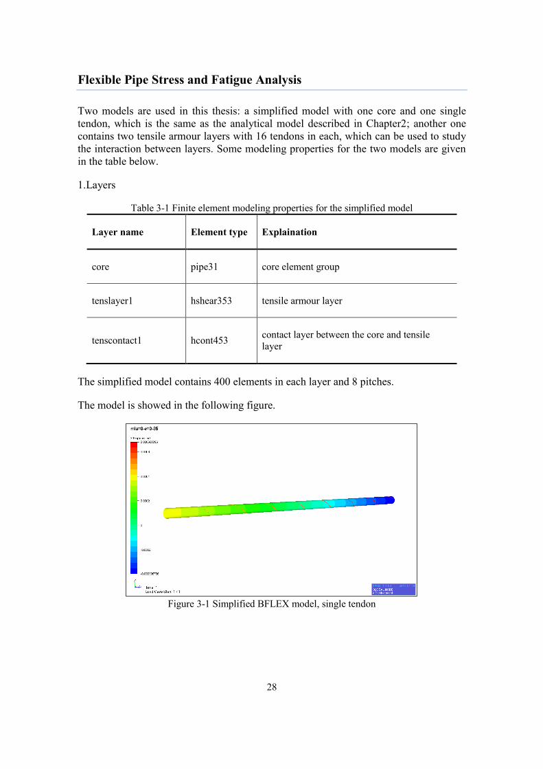
The simplified model contains 400 elements in each layer and 8 pitches.
The model is showed in the following figure.
Figure 3-1 Simplified BFLEX model, single tendon

Flexible Pipe Stress and Fatigue Analysis
29
Table 3-2 Finite element modeling properties for the model with two armour layers
Layer Element type Explaination
core pipe31 core element group
tenslayer1 hshear353 inner tensile armour layer
tenslayer2 hshear353 outer tensile armour layer
tenscontact1 hcont453 contact the supporting structure and inner
tesile armour layer
tenscontact1-2 hcont453 contact layer between two tensile armour
layers
layer2_outward spring137 contact layer between the second tensile
armour layer and the outer structure layer
The complex model contains 100 elements in each tendon. The inner layer contains 4
pitches and the outer layer contains 5. The model is shown in the following figure.
Figure 3-2 Complex BFLEX model, double tensile armour layers
2. Boundary condition

Flexible Pipe Stress and Fatigue Analysis
30
The rotation about x-axis is fixed for all layers, referring to the coordinate system in
figure2-13.The core is fixed in translation in x, y and z direction. Other boundary
conditions are applied for different cases as needed.
3. Material properties
The core is plastic and the tendon is elastic.
4. Other parameters
The following parameters are used: A global curvature 0.1 when exposed to
bending; a core with radius 0.1m; a rectangular tensile armour wire cross section 9×3
mm.
3.3.2 Finite element formulations for hshear353 and hcont453
In previous BFLEX finite element program system, the relative displacement in
transverse direction was neglected and the loxodromic path assumption was used. The
reason[9]
is that the transverse slip has been demonstrated to be small and has no
significant influence on the fatigue analysis regarding to the calculating the stress ranges
from local wire bending.
The main difference in this master thesis is that a new type of beam element hshear353
used to simulate tensile armour layer, together with a new type of contact layer element
hcont453 has been used. Thus, transverse slip regime is activated and can be
investigated. The aim of including transverse DOF is to study the wire buckling together
with end fitting effects and so on.
The models in this thesis are used as examples to demonstrate whether the developed
finite element formulation for the beam element hshear353 and the contact element
hcont453 can give adequate description of slip behaviour or not. This is done by
comparing the BFLEX result with the analytical solution on some simple cases.
Beam element – hshear353[10]
hshear353 element is a two nodes beam element with 26 DOFs: 12 associated to the
standard beam DOFs at the pipe center line used to describe the global strain quantities;
14 DOFs of the tensile layer which describe the local displacements of the wire relative
to the core. Cubic interpolation in all directions is applied which leads to the membrane
locking phenomena due to curvature coupling terms. A figure illustrates the DOFs is
give blow:

Flexible Pipe Stress and Fatigue Analysis
31
Figure 3-3 coordinate system for hshear353[10]
It should be noted that surface coordinate in the above figure is the same as as
defined before. Definition will still be used in the following.
The internal virtual work contribution for this element is[10]
:
∫ 𝐴( + ) + (
+ ) + ( +
) + ( + ) + ∙ ∙ ∙ 𝑑
(3.1)
Where are torsion and curvature quantities obtained from curved beam
theory[11]
as a result of relative sliding from the reference loxodromic curve. These
include coupling terms between current torsion and curvature and the displacements and
rotation of centerline[10]
.
represents the prescribed torsion and curvature quantities that would result if plane
surfaces remain plane and the wire strain, torsion and curvature being described by the
loxodromic curve quantities. Quantity represents the bi-directional relative
displacement between tendon and core along the helical path where the sandwich beam
theory is applied. C is a two-dimensional shear stiffness tensor determined by the stick-
slip condition between layers, reducing to zero in the slip domain.
If we assume small strains and the kinematic restraint in (2.16), the prescribed quantities
can be obtained as:

Flexible Pipe Stress and Fatigue Analysis
32
+ +
(3.2)
( + ) +
+
(3.3)
( )
+
( + ) (3.4)
( + ) ( ) (3.5)
It should be noted the transverse curvature к
is used here. It is because the
prescribed quantities are applied before bending and hence no contribution is given by
к .
are the transverse displacement components at the center of cross section,
represents the prescribed rotation quantities at the pipe centerline.
Contact element –hcont453[10]
The interlayer contact forces and the friction with regard to the relative displacement are
described by the contact element hcont453 in the new version of BFLEX2010. hcont453
contains 24 DOFs as illustrated in the figure below:

Flexible Pipe Stress and Fatigue Analysis
33
Figure 3-4 New contact element hcont453[9]
This element is based on a Hybrid Mixed formulation described in [11]-[12]. The basis
of the concept is the incremental potential formulated as:
∫( + ) ∙ 𝑑
∫
𝑑
∫ ∙ 𝑑
∫ ∙ 𝑑
(3.6)
Where is the distributed normal reaction, is the distributed tangential reaction
assuming a bi-directional friction model and is a penalty stiffness parameter.
The finite element includes the following key features[10]
:
1.Describing contact between layers of crossing tensile wires
2.Enabling easy description of the resistance against wire rotation from other layers by
including torsion coupling terms

Flexible Pipe Stress and Fatigue Analysis
34
Chapter4 Numerical studies
4.1 Introduction
One of the main purposes of this chapter is to study how the numerical solution can be
influenced by different parameters, e.g., friction coefficient, global curvature, cyclic
bending effect and so on. In addition, the numerical and analytical results are compared
for both axisymmetric loading case and bending. The aim of the comparisons is to
verify that the numerical model can give adequate description of the tendon’s stress and
slip behaviour.
First of all, a verification of the numerical model on axisymmetric behaviour is carried
out. The numerical solution for axisymmetric loading is compared with the analytical
result. Two analytical solutions, one by Sævik[2]
, one by Witz & Tan[13]
are compared
with BFLEX result.
Also, an investigation on the maximum local curvilinear displacements in terms of
friction coefficient, global curvature and strain under bending is carried out. The aim is
to find out how the local curvilinear displacements can vary as a function of the three
variables.
Moreover, the numerical model is compared with the analytical solution stated in
Chapter2.4 where the pipe exposed to constant curvature. The aim of this is to verify
that the numerical model can give successful description of the tendon’s kinematic
when subjected to bending.
Finally, the influence from cyclic bending effect on local curvilinear displacements is
carried out. Both simplified model and the model with double tensile layers are used.
Beam element hshear353 and contact element hcont453 are used throughout this
chapter. The control parameter for hcont453 is set to zero which means the friction
force acting between layers is dependent on each other, i.e., the interaction of friction
forces between layers is included.
4.2 Comparison on numerical and analytical solutions-
axisymmetric loading
4.2.1 Description of the problem
This example case compares two analytical solutions with the numerical result from
BFLEX2010 regarding axisymmetric loading, i.e., tension, torque and internal/external
pressure. On the one hand, this case is used to find out that which analytical solution can
better predict the motion of tendon, i.e., give closer result when comparing to numerical
solution. On the other hand, it can also be used to prove that the developed numerical
model can give adequate description of the tendon kinematic.

Flexible Pipe Stress and Fatigue Analysis
35
The simplified BFLEX model described in Chapter3 is used. Additional boundary
condition is that the tensile armour layer is fixed on axial and transverse displacements
at both ends.
4.2.2 Two analytical descriptions
Two existing analytical solutions are studied:
From Sævik[2]
:
The analytical description by Sævik is introduced in Chapter2.3. Eqs.(2.34)- (2.35)
regarding twist and normal curvature increment are used to represent the tendon’s
kinematic behaviour and hence compared with other solutions. This is because the
curvature increments have a linear relationship with local moment stress.
From Witz & Tan[13]
:
Witz & Tan suggest another method to describe axisymmetric loading; stated in
[13].The difference for their solution comparing to Sævik’s is that the center line
straining of the tendon is excluded by them. Their results are directly obtained by input
accumulated torsion and curvature which is expressed by updated lay angle and layer
radius into Eqs.(2.7)-(2.8). The formulas obtained from their reference are given in Eqs.
(4.1) - (4.2).
к
( ) + ( )𝜃 +
(4.1)
к
+ 𝜃 +
(4.2)
4.2.3 Comparison with numerical solution
In BFLEX2010, the Green strain theory and the Principle of virtual displacements
discussed in Chapter2 are used to calculate stress relations. The simplified model
discussed in Chapter3 is used.
Axial strain, torsion and radial displacements are applied to the model respectively.
Comparison on twist and normal curvature increments by using the above three methods
are carried out and discussed. Lay angles varying from 25°to 55°are studied. Initial
principal curvature for a constant pipe is subtracted and only the curvature increment is
shown in the plot.
Axial strain

Flexible Pipe Stress and Fatigue Analysis
36
Axial strain ( ), which represents tension, is applied from 0 to 0.01 within one hundred
load steps in BFLEX2010.
Curvature increments are plotted as a function of axial strain in the figures below.
Figure 4-1 Curvature increments as a function of axial strain- 25°lay angle
It is observed in the above figure that the difference between Sævik’s and BFLEX
solution is smaller than the difference between Witz&Tan’s and BFLEX solution. In all
solutions, curvature increase linearly to axial strain.

Flexible Pipe Stress and Fatigue Analysis
37
Figure 4-2 Curvature increments as a function of axial strain-35°lay angle
For 35°lay angle, it is found that the BFLEX solution increases rapidly when axial strain
exceeds 0.0045. It is because nonlinear effects become significant in the model as the
axial strain increases. For the region axial strain is smaller than 0.0045, linear
relationship between axial strain and curvature increment is found, and Sævik’s results
have smaller deviation to BFLEX results comparing to Witz&Tan’s.

Flexible Pipe Stress and Fatigue Analysis
38
Figure 4-3 Curvature increments as a function of axial strain-45°lay angle
Figure 4-4 Curvature increments as a function of axial strain-55°lay angle

Flexible Pipe Stress and Fatigue Analysis
39
For 45 and 55° lay angle, similar results are found as for 35° lay angle: When the axial
strain exceeds a certain value, the curvature increment is governed by non-linear effect
and thus none of the two analytical solutions can give adequate prediction. In the linear
region, Sævik’s solution gives closer results with numerical solution.
Torsion
This thesis tests the region of global torsion(𝜃 ) from 0 to 0.01( ), results are shown
in the figures below.
Figure 4-5 Curvature increments as a function of torsion-25°lay angle

Flexible Pipe Stress and Fatigue Analysis
40
Figure 4-6 Curvature increments as a function of torsion-35°lay angle
Figure 4-7 Curvature increments as a function of torsion-45°lay angle

Flexible Pipe Stress and Fatigue Analysis
41
Figure 4-8 Curvature increments as a function of torsion-55°lay angle
It is found that both twist and normal curvatures increase linearly as the global torsion
𝜽 𝒛 increases. Sævik’s solution gives very good prediction of the BFLEX results where
the blue solid line is almost overlapped with the red dash line. However, Witz&Tan’s
results show larger deviations.
Radial displacement
Radial displacement , which represents for internal/external pressure is applied from
0 to 0.001(m).

Flexible Pipe Stress and Fatigue Analysis
42
Figure 4-9 Curvature increments as a function of radial displacement-25°lay angle
Figure 4-10 Curvature increments as a function of radial displacement-35°lay angle

Flexible Pipe Stress and Fatigue Analysis
43
Figure 4-11 Curvature increments as a function of radial displacement-45°lay angle
Figure 4-12 Curvature increments as a function of radial displacement-55°lay angle

Flexible Pipe Stress and Fatigue Analysis
44
Sævik’s formulas give very close result to numerical result from BFLEX2010, while
Witz &Tan’s shows relative larger deviation.
All in all, the curvature increments obtained by Witz&Tan have larger deviations with
numerical solutions comparing to Sævik’s. It is because they express the accumulated
torsion and curvature by using the updated lay angle and layer radius. They insert the
accumulated quantities directly into Eq. (2.7)-(2.8) without taking the central line
straining into account.
4.3 Parameter study on local displacements under bending
4.3.1 Description of the problem
This example studies how the maximum displacement/curvature increments can be
influenced by certain pipe parameters, i.e., global curvature/friction coefficient/axial
strain when exposed to bending. The simplified BFLEX model with single tendon and
35°lay angle is studied as an example here.
In this case, the tensile layer in BFLEX model is fixed in x and y direction at one end
and have prescribed axial displacement, which is introduced by axial strain at the
other end in order to simulate tension in the pipe and avoid buckling. The axial strain is
applied before bending and the influence of this is further subtracted.
The aim of this sub-chapter is to find out that at which level of global curvature/friction
coefficient/axial strain, the maximum displacement/curvature increments become stable.
Those values are chosen when comparing BFLEX results with loxodromic solution in
chapter4.4.
4.3.2 Global curvature’s influence
In this case, friction coefficient and axial strain are assumed as given quantities, equals
0.05 and 0.0015 respectively. Maximum displacements/curvature increments are studied
regarding different global pipe curvatures: 0, 0.01, 0.0125, 0.02, 0.025, 0.05, 0.1( ), Initial principal curvature for a straight pipe and increments induced by axial strain are
subtracted.
The results are given below:

Flexible Pipe Stress and Fatigue Analysis
45
Figure 4-13 Maximum longitudinal displacement as a function of global pipe curvature
Figure 4-14 Maximum transverse displacement as a function of global pipe curvature
Figure 4-15 Maximum twist curvature increment as a function of global pipe curvature

Flexible Pipe Stress and Fatigue Analysis
46
Figure 4-16 Maximum transverse curvature increment as a function of global pipe curvature
Figure 4-17 Maximum normal curvature increment as a function of global pipe curvature
The results show that displacements/curvatures increase linearly as global pipe
curvature increases. In the thesis, a 0.1 global curvature for later tests is used.
This is in order to make sure that the slip behaviour is governed by the bending process
instead of axial stiffness.
4.3.3 Friction coefficient’s influence
Now the maximum displacements/curvature increments are tested with varying friction
coefficient: 0, 0.05, 0.1, 0.2, 0.3, 0.4, 0.5. Axial strain 0.0015, global curvature 0.1
are applied. Increments induced by axial strain are subtracted.

Flexible Pipe Stress and Fatigue Analysis
47
Figure 4-18 Maximum longitudinal displacement as a function of friction coefficient
The x-axis label ‘miu’ in the figure above represents for friction coefficient. It is stated
in Chapter2 that the longitudinal slip depends on the axial strain from the compressive
side to the tensile side and thus not much influenced by friction coefficient, which
Figure 4-18 shows consistent result.
Figure 4-19 Maximum transverse displacement as a function of friction coefficient
The analytical solution stating that transverse displacement will be prohibited by
friction is approved by numerical result showed in figure 4-19: the transverse slip is
reduced rapidly as friction coefficient increases and soon become a negligible value.

Flexible Pipe Stress and Fatigue Analysis
48
Figure 4-20 Maximum twist curvature increment as a function of friction coefficient
Figure 4-21 Maximum transverse curvature increment as a function of friction coefficient
At the meantime, transverse curvature is eliminated by transverse slip when the friction
coefficient is small as described in figure 4-21.
Figure 4-22 Maximum normal curvature increment as a function of friction coefficient

Flexible Pipe Stress and Fatigue Analysis
49
The transverse displacement and other curvature increments tend to become constant
when friction coefficient becomes larger than 0.3. Thus, when comparing the numerical
and loxodromic solution in Chapter4.4, the BFLEX result with friction coefficient 0.3 is
used.
4.3.4 Axial strain’s influence
Axial strain is applied in order to make sure the tendon is subjected to tension and such
avoid buckling. In this part, maximum displacements/curvature increments with
different global pipe axial strains: 0.001, 0.0015, 0.002, 0.003, 0.004, 0.005 are studied.
Friction coefficient 0.05 and global pipe curvature 0.1 is applied. 35°lay angle is
used as an example here.
Figure 4-23 Maximum longitudinal displacement as a function of axial strain
It is observed from the above figure that the longitudinal displacement is not much
influenced by axial strain when the axial strain changes from 0 to 0.005. It could be
explained by that this effect is governed by axial force along the tendon which
developed from the compression side to the tensile side, but not global tension.
Figure 4-24 Maximum transverse displacement as a function of axial strain

Flexible Pipe Stress and Fatigue Analysis
50
Figure 4-25 Maximum twist curvature increment as a function of axial strain
Figure 4-26 Maximum transverse curvature increment as a function of axial strain
Figure 4-27 Maximum normal curvature increment as a function of axial strain
All the displacements/curvature increments are not varying too much when axial strain
is larger than 0.001. Thus, axial strain 0.0015 is used in the numerical model in

Flexible Pipe Stress and Fatigue Analysis
51
Chapter4.4 and compared with the analytical solution. Other reasons to use axial strain
0.0015 are that it provides reasonable axial stress as used in real life and the numerical
model converges faster within this value.
4.4 Comparison on numerical and analytical solutions-bending
4.4.1 Description of the problem
The aim of this sub-chapter is to verify that whether the numerical model can provide
adequate description of the pipe bending behaviour or not. Comparison between
BFLEX numerical simulations and analytical results with the help of the model
described in Chapter2.4 is carried out.
Both simplified and complex BFLEX models are used and the pipe is bent step by step
from straight to a constant global curvature 0.1( ). It should be noted that the
complex model has only half-length of the simplified model. The inner layer of the
complex model has the same lay-angle as the simplified model with 4 pitches while the
simplified model has 8.
Two groups of comparison are carried out, namely:
1. The geodesic solution: referring to Eqs. (2.38)-(2.41), is compared with the
BFLEX solution with 0 friction and 0.0015 axial strain;
2. The loxodromic solution: referring to Eqs. (2.42)-(2.44), is compared with the
BFLEX result where friction coefficient equals 0.3 with 0.0015 axial strain.
The friction coefficient, axial strain and global curvature used here are chosen based on
experiments in Chapter4.3. Local displacements and curvature increments induced by
bending are studied. Axial strain is applied before bending and the influence is
subtracted when plotting the figures in this sub-chapter. Initial principal curvature for a
constant pipe is further deducted and only the curvature increments are studied.
4.4.2 Discussion of the results
The slip/curvature increments during bending are studied for different lay angles from
25°to 55°as showed below, where ‘miu’ in the figure represents friction coefficient used
in BFLEX simulation. For the complex model, the results are taken out from the inner
tendon. The figures marked with “16 tendons” are results from the inner layer of the
complex model.
Longitudinal slip
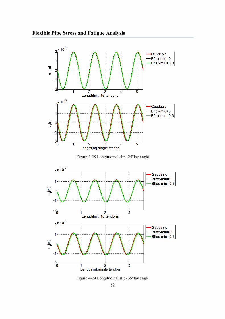
Flexible Pipe Stress and Fatigue Analysis
52
Figure 4-28 Longitudinal slip- 25°lay angle
Figure 4-29 Longitudinal slip- 35°lay angle

Flexible Pipe Stress and Fatigue Analysis
53
Figure 4-30 Longitudinal slip- 45°lay angle
Figure 4-31 Longitudinal slip- 55°lay angle

Flexible Pipe Stress and Fatigue Analysis
54
From Figure4-28 to Figure4-31, it is observed that the longitudinal slip is independent
on friction force. This gives agreement with the statement in Chapter2: the longitudinal
slip is governed by the axial strain developed in the tendon from compression side to
tension side induced by bending but not friction force.
It is further found that the longitudinal slip is not influenced by the outer tensile armour
layer as the longitudinal displacements are same for both models and all lay angles.
The maximum longitudinal slip reduces as the lay angle increases as illustrated by the
following figure:
Figure 4-32 Maximum longitudinal slip as a function of lay angle
Transverse slip
Transverse slips along the tendon are plotted for different lay angles:
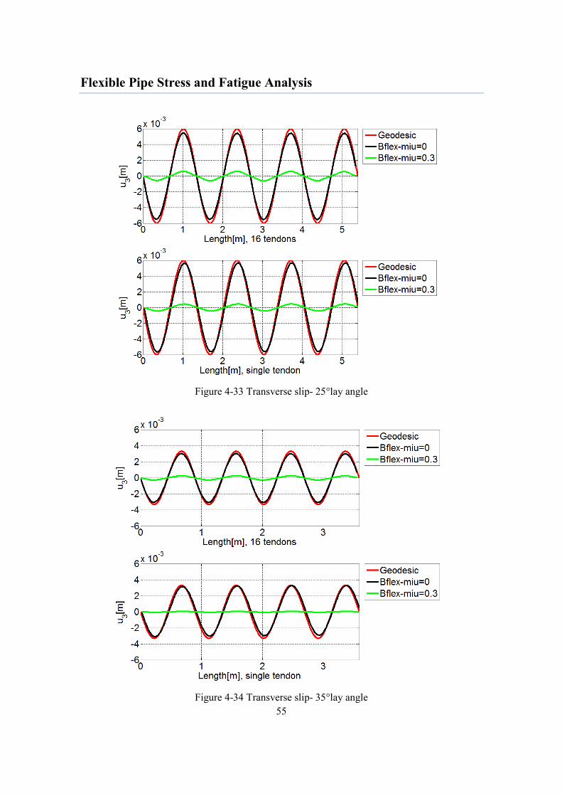
Flexible Pipe Stress and Fatigue Analysis
55
Figure 4-33 Transverse slip- 25°lay angle
Figure 4-34 Transverse slip- 35°lay angle

Flexible Pipe Stress and Fatigue Analysis
56
Figure 4-35 Transverse slip- 45°lay angle
Figure 4-36 Transverse slip- 55°lay angle

Flexible Pipe Stress and Fatigue Analysis
57
As described in Chapter2.4, transverse curvature will occur under loxodromic
assumption when the pipe is subjected to bending. A transverse slip will start if zero
friction condition is assumed. Tendon will in this way follows the geodesic assumption.
When the friction is large enough, transverse slip will be restraint and the tendon will
follow the loxodromic path.
The BFLEX results with zero friction give harmonic solutions which are consistence
with the geodesic solution stated in Eq. (2.39). The transverse slip amplitude simulated
by BFLEX matches well with the geodesic solution. However, a difference in mean
value is observed for large lay angles for the simplified model. This is introduced by the
prescribed displacements.
It is observed the transverse slip is very small for friction coefficient 0.3 in BFLEX. The
results match the loxodromic assumption: transverse slip is prohibited by friction force.
It is observed that the out armour layer does not influence the transverse slip
significantly.
Figure 4-37 Maximum transverse slip as a function of lay angle
Refer to figure 4-37, the amplitude of transverse slip reduces as the lay angle increases
when friction coefficient is set to zero. While the transverse slip reduces to almost zero
for all lay angle with large friction. The increase in maximum transverse slip for the

Flexible Pipe Stress and Fatigue Analysis
58
simplified model with zero friction at 55°lay angle is because the increase in mean value
as stated in figure 4-36.
Twist curvature increment
Figure 4-38 Twist curvature increment- 25°lay angle

Flexible Pipe Stress and Fatigue Analysis
59
Figure 4-39 Twist curvature increment- 35°lay angle
Figure 4-40 Twist curvature increment- 45°lay angle

Flexible Pipe Stress and Fatigue Analysis
60
Figure 4-41 Twist curvature increment- 55°lay angle
Figure 4-42 Maximum twist curvature increment as a function of lay angle

Flexible Pipe Stress and Fatigue Analysis
61
It is concluded from the above figures that the BFLEX solution matches well with
geodesic solution when friction coefficient is set to zero. A sign change around 35°lay
angle in both solutions is observed. For the geodesic solution, this is introduced by
(
)term in Eq.(2.40). The BFLEX results reflect this change of sign and thus
approve geodesic solution.
However, the BFLEX result with 0.3 friction coefficient is larger than the loxodromic
solution for all lay angles. This is explained by the following.
The loxodromic curvature increments (2.42) and (2.44) are deduced on the basis that no
slip occurs during bending. However, a longitudinal slip (2.38) will always be
introduced in order to eliminate longitudinal strain. In BFLEX result with 0.3 friction
coefficient, the curvature increment is calculated after this longitudinal slip. Thus, in
order to include the influence from longitudinal slip and compare with BFLEX result,
equation (2.42) which represents for curvature increment without any slip, should be
added an extra term which including longitudinal slip in [2].
According to [2], by using kinematic restraint Eq.(2.16) and assume 2D effect, the twist
curvature increments induced by longitudinal slip using loxodromic curve as reference:
к к (4.3)
By including the influence induced by longitudinal slip, i.e., adding Eq.(4.3) to the
loxodromic solution (2.42), the twist curvature change along the pipe is shown in the
figure below:

Flexible Pipe Stress and Fatigue Analysis
62
Figure 4-43 Modified twist curvature increment-25°lay angle
Figure 4-44 Modified twist curvature increment- 35°lay angle

Flexible Pipe Stress and Fatigue Analysis
63
Figure 4-45 Modified twist curvature increment- 45°lay angle
Geodesic, loxodromic and BFLEX results are overlapped for 45°lay angle.
Figure 4-46 Modified twist curvature increment- 55°lay angle

Flexible Pipe Stress and Fatigue Analysis
64
Maximum curvature changes hence become:
Figure 4-47 Maximum twist curvature change with longitudinal slip, modified
Here we can conclude that the twist curvature for BFLEX with friction agrees with
loxodromic solution which including the additional influence from longitudinal slip.
Transverse curvature increment

Flexible Pipe Stress and Fatigue Analysis
65
Figure 4-48 Transverse curvature increment- 25°lay angle
Figure 4-49 Transverse curvature increment- 35°lay angle

Flexible Pipe Stress and Fatigue Analysis
66
Figure 4-50 Transverse curvature increment- 45°lay angle
Figure 4-51 Transverse curvature increment- 55°lay angle

Flexible Pipe Stress and Fatigue Analysis
67
From Figure4-48 to Figure4-51, the loxodromic solutions agree well with the BFLEX
solutions when miu=0.3. A small transverse curvature is observed for BFLEX solution
where friction is assumed to be zero. Such a small curvature could be neglected and can
be concluded that the BFLEX solution matches the geodesic solution very well.
Figure 4-52 Maximum transverse curvature increment as a function of lay angle
It is found from above figure; transverse curvature increment is not influenced by lay
angle.
Normal curvature increment

Flexible Pipe Stress and Fatigue Analysis
68
Figure 4-53 Normal curvature increment- 25°lay angle
Figure 4-54 Normal curvature increment- 35°lay angle

Flexible Pipe Stress and Fatigue Analysis
69
Figure 4-55 Normal curvature increment- 45°lay angle
Figure 4-56 Normal curvature increment- 55°lay angle

Flexible Pipe Stress and Fatigue Analysis
70
The geodesic solutions and BFLEX solutions give good agreement with each other as
observed in Figure 4-53 to Figure 4-56.
However, the difference between loxodromic solution and numerical simulation
increases as the lay angle increases. Even an opposite sign is observed between
loxodromic and BFLEX result for 55°lay angle. This could be explained in the same
way for the twist curvature: the difference is introduced by the longitudinal slip which is
not included in the loxodromic solution Eq.(2.44). By including the longitudinal slip’s
influence on normal curvature, an additional term should be added to Eq.(2.44)[2]
:
к к (4.4)
The new loxodromic solution by including Eq.(4.4) in is plotted in the figure below:
Figure 4-57 Modified normal increment- 25°lay angle

Flexible Pipe Stress and Fatigue Analysis
71
Figure 4-58 Modified normal increment- 35°lay angle
Figure 4-59 Modified normal curvature increment- 45°lay angle

Flexible Pipe Stress and Fatigue Analysis
72
Figure 4-60 Modified normal curvature increment- 55°lay angle
From the above four figures, it is found the BFLEX results match the loxodromic
solution very well by including the influence due to longitudinal slip. No significant
influence from the outer armour layer in the complex model is observed.
The normal curvatures decrease as the increase of lay angles, maximum normal
curvature increments for different lay angles are plotted in the figure below:
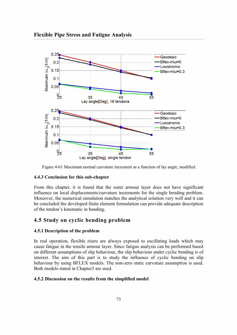
Flexible Pipe Stress and Fatigue Analysis
73
Figure 4-61 Maximum normal curvature increment as a function of lay angle, modified
4.4.3 Conclusion for this sub-chapter
From this chapter, it is found that the outer armour layer does not have significant
influence on local displacements/curvature increments for the single bending problem.
Moreover, the numerical simulation matches the analytical solution very well and it can
be concluded the developed finite element formulation can provide adequate description
of the tendon’s kinematic in bending.
4.5 Study on cyclic bending problem
4.5.1 Description of the problem
In real operation, flexible risers are always exposed to oscillating loads which may
cause fatigue in the tensile armour layer. Since fatigue analysis can be performed based
on different assumptions of slip behaviour, the slip behaviour under cyclic bending is of
interest. The aim of this part is to study the influence of cyclic bending on slip
behaviour by using BFLEX models. The non-zero static curvature assumption is used.
Both models stated in Chapter3 are used.
4.5.2 Discussion on the results from the simplified model

Flexible Pipe Stress and Fatigue Analysis
74
The simplified model with only a core and a single tendon is studied here. The pipe is
forced to be bent from straight to a constant global curvature 0.1( ) and then back
to straight. This procedure is repeated for several times. The influencing parameters that
will be studied are axial strain and friction coefficient.
Axial strain’s influence
First, the influence from axial strain on cyclic bending is studied. 45°lay angle and
friction coefficient 0.15 are used in the simplified BFLEX model. Initial axial strain is
applied at first ten seconds, and then the pipe is bent with a period 40 seconds per cycle.
The twist and normal curvatures at the tension side in the middle of the pipe are studied.
BFLEX increment
Loxodromic increment
Geodesic solutions
Loxodromic solutions
Figure 4-62 Twist curvature as a function of time, axial strain’s influence
In figure 4-62, the three black lines represent for the Geodesic solutions. The thick one
in the middle represents geodesic solution (Eq. (2.40))with half global pipe curvature,
i.e., curvature 0.05( ), plus the principal curvature for a straight pipe( Eq.(2.7)). The
other two thinner ones represent for the plus and minus geodesic increments with
curvature 0.1( ) in addition to the thick black line.
The three blue lines represent for the Loxodromic solutions. Similarly, the thick blue
line in the middle represents for loxodromic solution (Eq.(2.42)) with half global
curvature plus the principal curvature valid for a straight pipe. The other two blue lines
represent for the plus and minus loxodromic increment with curvature 0.1( ) in
addition to the thick blue line.
In figure 4-62, it is observed that twist curvature increment does not vary from cycle to
cycle and agrees with the loxodromic assumption as indicated by the arrows.
The mean twist curvature does not change along time series and can be explained by
that the tendon is still in elastic range in this direction.
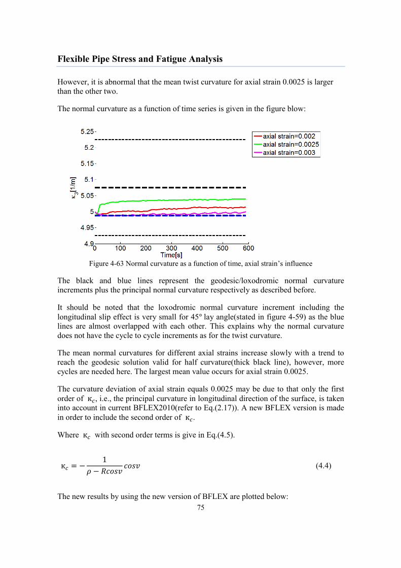
Flexible Pipe Stress and Fatigue Analysis
75
However, it is abnormal that the mean twist curvature for axial strain 0.0025 is larger
than the other two.
The normal curvature as a function of time series is given in the figure blow:
Figure 4-63 Normal curvature as a function of time, axial strain’s influence
The black and blue lines represent the geodesic/loxodromic normal curvature
increments plus the principal normal curvature respectively as described before.
It should be noted that the loxodromic normal curvature increment including the
longitudinal slip effect is very small for 45 lay angle(stated in figure 4-59) as the blue
lines are almost overlapped with each other. This explains why the normal curvature
does not have the cycle to cycle increments as for the twist curvature.
The mean normal curvatures for different axial strains increase slowly with a trend to
reach the geodesic solution valid for half curvature(thick black line), however, more
cycles are needed here. The largest mean value occurs for axial strain 0.0025.
The curvature deviation of axial strain equals 0.0025 may be due to that only the first
order of к , i.e., the principal curvature in longitudinal direction of the surface, is taken
into account in current BFLEX2010(refer to Eq.(2.17)). A new BFLEX version is made
in order to include the second order of к .
Where к with second order terms is give in Eq.(4.5).
к
(4.4)
The new results by using the new version of BFLEX are plotted below:

Flexible Pipe Stress and Fatigue Analysis
76
Figure 4-64 Twist curvature as a function of time, axial strain’s influence, modified
Figure 4-65 Normal curvature as a function of time, axial strain’s influence, modified
It is observed from the above figures that the mean twist curvature for axial strain
0.0025 is now between the two for axial strain 0.002 and 0.003. This means the twist
curvature become more reasonable by including the second order terms in к .
Moreover, the differences for normal curvature among the three axial strains are
smaller. However, the mean normal curvature for axial strain 0.0025 is still larger than
the other two.
In this part, only a simple case with 45 lay angle and friction coefficient 0.15 has been
studied. This is because those values are corresponding to real flexible pipe operation.
What’s more, convergence problem is found for current BFLEX input file for some
other lay angles.

Flexible Pipe Stress and Fatigue Analysis
77
Friction’s influence
(1) 35°lay angle
A model with 35°lay angle and axial strain 0.0025 is first used. Axial strain is applied
during the first 10 seconds and cyclic bending with period 40 seconds is applied
afterwards. The twist and normal curvatures at the tension side in the middle of the pipe
are plotted below.
Loxodromic increment
Bflex increment
Figure 4-66 Twist curvature as a function of time, friction’s influence
Loxodromic increment
Bflex increment
Figure 4-67 Normal curvature as a function of time, friction’s influence
In figure 4-66 and 4-67, the blue lines and black lines represents the same meaning as
described before. One should note that the geodesic solution for twist curvature

Flexible Pipe Stress and Fatigue Analysis
78
increment is very small for 35 lay angle (figure 4-44), so the three black lines become
very close to each other in figure 4-66.
It can be concluded that the cyclic curvature increments follows the loxodromic
assumption as indicated by the arrows.
In addition, it is observed that the friction coefficient does not have significant influence
on cycle to cycle curvature increments in this case. However, an influence on mean
curvatures is observed: the mean curvature quantities are a bit larger for friction
coefficient 0.15 than for 0.3.
It is also found that the mean twist and normal curvatures increase along time axis. The
increments show a tendency to reach the thick black line, i.e., the geodesic solution
valid for half curvature plus the principal curvature. This is reasonable as the pipe is
bent from straight to a certain curvature and then back to straight. In figure 4-67, the
mean normal curvature increases slowly and does not reach a stable value at the end of
time series. It shows that more than ten cycles are needed to reach stable for both
curvatures.
(2) 45°lay angle
In addition, a study for 45 lay angle is carried out. Friction coefficient 0.1 and 0.2 are
chosen based on convergence requirement in BFLEX. Results are given in figures
below:
Loxodromic increment
Bflex increment
Figure 4-68 Twist curvature as a function of time, friction’s influence
It can be concluded from the above figure that the mean twist curvature for 45 lay
angle does not vary with time. This is consistent with result from figure 4-62 and can be
explained by that the pipe is still in elastic range here. The cyclic increment of twist

Flexible Pipe Stress and Fatigue Analysis
79
curvature simulated by BFLEX gives agreement with the loxodromic solution, as
indicated by the arrows.
Again, friction coefficient does not have any influence on cycle to cycle increment but
has influence on mean curvature.
Figure 4-69 Normal curvature as a function of time, friction’s influence
For normal curvature, an increase in mean value for miu=0.2 is observed. However, the
mean value for miu=0.1 decreases during cyclic bending. The cyclic increment is
consistent with the loxodromic assumption as it is very small for 45 lay angle.
This case with 45 lay angle is further tested by using the new version of BFLEX by
including the second order term for к , the results are given below.
Figure 4-70 Twist curvature as a function of time, friction’s influence, modified

Flexible Pipe Stress and Fatigue Analysis
80
A decrease in mean twist curvature for friction coefficient 0.2 is observed under the
influence of the second order term of к .
Figure 4-71 Normal curvature as a function of time, friction’s influence, modified
It can be concluded from figure 4-70 and 4-71 that the second order term of к has
significant influence on twist and normal curvatures.
4.5.2 Discussion on the results from the complex model
The complex model with two tensile armour layers is used in this case. For the complex
model, the inner layer contains 4 pitches and has lay angle 35 , the outer layer contains
5 pitches and has lay angle 42 . Initial axial strain is applied at first ten seconds, cyclic
bending with period 20 seconds is applied afterwards. Cyclic bending effects on inner
and outer layer are studied respectively.
First, the curvature quantities for the inner layer are studied. The curvature increments
are taken out at the middle of the tensile side, i.e., where the maximum increments
occur.

Flexible Pipe Stress and Fatigue Analysis
81
Loxodromic increment
Bflex increment
Figure 4-72 Twist curvature as a function of time, inner layer
Loxodromic increment
Bflex increment
Figure 4-73 Normal curvature as a function of time, inner layer
The black and blue lines represent the geodesic and loxodromic solutions with different
global curvature as indicated previously.
It is observed that both mean twist and normal curvatures increase as a function of time
and tend to reach the geodesic solution (thick black line) valid for half global curvature
plus principal curvature after a few cycles. Fewer cycles are needed to reach the stable
mean value comparing to the simplified model.
It is also found that the curvature increments from cycle to cycle calculated by
loxodromic assumption are consistent with the BFLEX’s increment as indicated by the
arrows.

Flexible Pipe Stress and Fatigue Analysis
82
For the outer layer, results are taken from the middle of the pipe at the tensile side, as
given below:
Loxodromic increment
Bflex increment
Geodesic increment
Figure 4-74 Twist curvature as a function of time, outer layer
It is observed that the twist curvature increment for the outer layer follows the geodesic
solution at beginning. The increment increases from cycle to cycle and approximately
reaches the loxodromic solution after many cycles. The curvature increment does not
reach its stable value and more cycles are suggested to be included.
In addition, the mean twist curvature does not change from cycle to cycle for the outer
layer.
The normal curvature increment as a function of time is given below:
Geodesic increment
Bflex increment
Figure 4-75 Normal curvature as a function of time, outer layer

Flexible Pipe Stress and Fatigue Analysis
83
Similar to twist curvature increment, the normal curvature increment follows the
geodesic solution at beginning. The increment decreases and tends to reach the
loxodromic solution after many cycles. However, many cycles are needed in order to
reach a stable normal curvature. Again, the mean normal curvature does not vary with
time.

Flexible Pipe Stress and Fatigue Analysis
84
Chapter 5 Summery
5.1 Conclusions
The main purpose of this thesis is to study the stress and slip behaviour for non-
bonded flexible pipes. Numerical studies are carried out both to verify the model by
comparing the numerical results with analytical results and to study various physical
effects. The main advantage of this thesis is the application of two new element types
in BFLEX2010, namely hshear353 and hcont453 which include the transverse
degrees of freedom of the tendon.
For flexible pipes exposed to axisymmetric loading, two analytical methods, one
obtained from the reference by Witz&Tan[13]
, one from Sævik[2]
, are compared with
the numerical result from BFLEX. It has been concluded that Sævik’s method gives
better agreement with BFLEX result comparing to Witz&Tan’s.
For flexible pipes exposed to bending, important parameters that can significantly
affect the slip behaviour (e.g., global pipe curvature, friction coefficient and axial
strain) have been studied. The simplified BFLEX model with single tendon is used.
When studying one of these parameters, the other two are fixed to a certain value.
The result shows that the tendon’s local displacements and curvature increments have
linear relationship with global curvature. When friction coefficient is within the range
from 0 to 0.3 or axial strain from 0 to 0.001, local displacements and curvature
increments are significantly influenced (either increased or decreased). For larger
friction coefficient or axial strain, local displacements and curvature increments tend
to be constant.
Furthermore, comparison between numerical simulation and analytical solution for
bending has been performed. For a single bending process, i.e., from straight to a
constant curvature, it has been concluded that the numerical solutions match well
with analytical solutions for either a simplified BFLEX model with single tendon or a
complex model with double tensile layers. It has been demonstrated that the
slip/curvature increments in the inner layer are not influenced by the outer tensile
layer during a simple bending procedure.
At last, cyclic bending effects on local curvature increments have been studied with
different BFLEX models.
For the simplified model with only one tendon, it has been found that cyclic
twist/normal curvature increments obtained from numerical simulation have good
agreement with the loxodromic assumption for 35 and 45 lay angles. The mean
twist and normal curvatures for 35 lay angle and the mean normal curvature for 45 lay angle increase as a function of time and show a tendency to reach the geodesic

Flexible Pipe Stress and Fatigue Analysis
85
solution valid for half curvature after many cycles. It should be noted the twist
curvature for 45 lay angle does not have this increment since it is in the elastic
range.
It has been found the friction coefficient does not have significant influence on cycle
to cycle curvature increments in this case. However, influence on mean curvatures is
observed. In addition, it has been noted that the second order effect of the surface
principal curvature in longitudinal direction has important influence on the mean
curvature.
For the test of the complex model with double tensile armour layers, the one with 35 inner layer lay angle and 42 outer layer lay angle has been used. The pipe
parameters are chosen based on a convergence requirement from BFLEX.
Convergence difficulties are found for some pipe parameters.
For the inner layer, it has been observed that the mean curvatures increase as a
function of time. The mean curvatures for this case increase faster than for the
simplified model. It has been observed that approximately only five cycles are needed
to reach the stable mean curvatures. At the same time, the loxodromic solutions have
good agreement with BFLEX results for cycle to cycle curvature increments.
For the outer layer, the mean curvatures do not vary as a function of time. The cyclic
curvature increments have started from geodesic solution and tended to reach the
loxodromic solution after many cycles.
5.2 Suggestions for future work
The cyclic bending effects have only been studied for some simple cases because
convergence problems have been found for some friction coefficients and axial strain
values. It is suggested that the model should be further improved and, as long as the
convergence problem has been solved, studies on cyclic bending regarding the
influence from different friction coefficients, axial strains, and lay angles can be
carried out and compared.
Further, for the model contains two tensile armour layers, the influence from the outer
layer on several things can be carried out: the influence on curvature increment of the
tendon, the influence on the relative displacement of the contact element, the
influence on local bending stress and so on.

Flexible Pipe Stress and Fatigue Analysis
86
Reference
[1] Berge,S., Engseth,A., Fylling,I., Larsen,C,M., Leira,B,J. and Olufsen,A.,1992.
“Handbook on design and operation of flexible pipes”. FPS2000, 1992.
[2] Sævik,S.,1992. “On stresses and fatigue in flexible pipes”. PhD thesis, NTH
Trondheim, Norway.
[3] B,Yong.,B,Qiang. SUBSEA PIPELINES AND RISERS. Elsevier, London, 1st edition,
2005.
[4] API. Ansi/api recommended practice 17b, 2008. Technical Report 4. Edition,
ANSI/API.
[5] Efficient Fatigue analysis of helix elements in umbilicals and flexible risers.
[6] Eisenhart, L.P.: “A Treatise on the differential Geometry of Curves and Surfaces”,
Dover Publ. Inc., 1960
[7] Feret, J.J, Bournazel, C.L.: “Calculation of Stresses and Slip in Structural Layers of
Unbounded Flexible Pipes”, Proc. of the Offshore Mechanics and Arctic Engineering
Conference, OMAE, 1986.
[8] Sævik,S. BFLEX2010- theory manual. MARINTEK, 2010.
[9] Sævik,S., J.Thosrsen,Mats. DRAFT: “Techniques for predicting tensile armour
buckling and fatigue in deep water flexible risers.” To be published, Proc. of the
Offshore Mechanics and Arctic Engineering Conference, OMAE, 2012.
[10] Sødahl,N.,1990. “Methods for design and analysis of flexible risers”. PhD thesis,
Norwegian University of Science and Technology, Trondheim, Norway.
[11] Shyu, S. C., Chang, T. Y., and Saleeb, A. F., 1987. “Finite element solutions of
two-dimensional contact problems based on a consistent mixed formulation”.
Computers and Structures, 27(4), pp. 455-466.
[12] Shyu, S. C., Chang, T. Y., and Saleeb, A. F., 1988. “Friction-contact analysis using
a mixed finite element method”. Computers and Structures, 27(4), pp. 223-242.
[13] Witz, J.A. and Tan, Z,. “On the axial-torsional structural behaviour of flexible
pipes, umbilicals and marine cables”, Marine Structures, vol5, pp205-227, 1992.
[14] Sævik,S., “ Theoretical and experimental studies of stresses in flexible pipes”.
Computers and Structures, 89 (2011) 2273-2291.
[15] API. Ansi/api recommended practice 17j, 2008. Technical Report 3. Edition,
ANSI/API.
Flexible Pipe Stress and Fatigue Analysis
87
[16] Sævik,S. BFLEX2010- user manual. MARINTEK, 2010.

i
Appendix A
BFLEX2010 input file for the simplified model:
#
HEAD #Text
#---------------------------------------------------------------------------
# Control data
#
# maxit ndim isolvr npoint ipri conr gacc iproc
CONTROL 100 3 2 16 11 1.e-5 0.0 stressfree
#CONTROL 100 3 1 16 11 1.e-5 9.81 restart 70
DYNCONT 1 0.0 0.09 -0.05
# t dt dtvi dtdy dt0 type hla?
#TIMECO 1.0 1.0 1.0 100.0 STATIC auto go-on disp 50
5 1e-5
TIMECO 100.0 1.0 10.0 100.0 static auto go-on disp 20
5 1e-5
#TIMECO 100.0 0.10 2.0 100.0 dynamic auto go-on disp 20
5 1e-5
#
#---------------------------------------------------------------------------
# Nocoor input
#
# no x y z
Nocoor Coordinates
1 0.0 0.0 0.0
401 #len 0.0 0.0
#
# no x0 y0 z0 b1 b2 b3 R node xcor theta
Nocoor Polar 0.0 0.0 0.0 0.0 0.0 0.0 0.100
1001 0.00 3.1416
1401 #len 53.4071
#
#
# no x0 y0 z0 b1 b2 b3 R node xcor theta
Nocoor Polar 0.0 0.0 0.0 0.0 0.0 0.0 0.100
20001 0.00 3.1416
20401 #len 53.4071
#
Visres Integration 1 Sigma-xx-ax Sigma-xx-my Sigma-xx-mz
#
#
#------------------------------------------------------------------------
# Elcon input
#
#
# The core
#
# group elty material no n1 n2 n3 n4
Elcon core pipe31 plastic 1 1 2
# n elinc nodinc
Repeat 400 1 1
#

ii
# Tensile Layer 1
# group elty flexcrossname no n1 n2 n3 n4
Elcon tenslayer1 hshear353 tendon 20001 1 2 20001 20002
# n elinc nodinc
Repeat 400 1 1
#
# Contact tensile Layer 1
# group elty flexcrossname no n1 n2 n3 n4
Elcon tenscontact1 hcont453 contmat1 50001 1001 1002 20001 20002
# n elinc nodinc
Repeat 400 1 1
#
#---------------------------------------------------------------------------
# Orient input
#
# The core
# no x y z
Elorient Coordinates 1 0 1e3 0
400 0 1e3 0
#
# no x y z
# Tensile Layer 1
# no x y z
Elorient Coordinates 20001 0 1e3 0
20400 0 1e3 0
elorient eulerangle 50001 0.0 0.0 0.0
50400 0.0 0.0 0.0
#
#
# groupn mname sname is1 isn istx isty istz gt1
gt2
# 1
means that friction is independent (tape between layers) else (isotropic model)
CONTINT tenscontact1 core tenslayer1 1 3 10 10 0 60 1
#--------------------------------------------------------------------------------
#
#------------------------------------------------------------------
#
# Element property input
#
# name type rad th CDr Cdt CMr CMt wd ws ODp ODw
rks
ELPROP core pipe 0.0985 0.001 1.0 0.1 2.0 0.2 500.00 0.00 0.197 0.197 0.5
# b t md ms scale thims thimd
iop iop=1 turn off axisymmetric shear inetraction =2 turn off bending shear interaction
ELPROP tenslayer1 shearhelix rectangle 0.009 0.003 1.4 0.0 1.0 200 100 0
# gap0 tunetime AUTOMNPC
ELPROP tenscontact1 layercontact d d d 0
# name type shearm
# Boundary condition data
# Loc node dir
BONCON GLOBAL 1 1
BONCON GLOBAL 1 2
BONCON GLOBAL 1 3
BONCON GLOBAL 1 4 repeat 401 1
BONCON GLOBAL 401 2

iii
BONCON GLOBAL 401 3
# fix the relative disp at ends
BONCON gLObAL 20001 1
BONCON gLObAL 20001 2
BONCON gLObAL 20001 4 repeat 401 1
#
BONCON gLObAL 1001 1 repeat 401 1
BONCON gLObAL 1001 2 repeat 401 1
BONCON gLObAL 1001 3 repeat 401 1
BONCON gLObAL 1001 4 repeat 401 1
BONCON gLObAL 1001 5 repeat 401 1
BONCON gLObAL 1001 6 repeat 401 1
#----------------------------------------
#-----------------------------------------------
#
# Constraint input
CONSTR PDISP GLOBAL 20401 1 #len*#as*#ca 300
CONSTR PDISP GLOBAL 20401 2 #len*#as*#sa 300
#
#---------------------------------------------
# Cload input
#
# hist dir no1 r1 no2 r2 n m
#
#CLOAD 300 1 51 270000.00
#piload 300 1 3e6 50 3e6
inistr 400 5 1 #strain 400 #strain
#---------------------------------------------
#PELOAD 200 100
#-----------------------------------------------------------
# History data
# force
THIST 100 0 0.0
1 0.00
10 0.00
THIST 200 0 0.0
1 0.00
10 0.00
THIST 300 0 0.0
10 1.00
100 1.00
THIST 400 0 0.00
10 0.00
100 1.00
# prescribed displacement
THIST_R 400 0.0 0.0 rampcos 0.0
0.0 0.0 rampcos 1.0
# 11.0 20.0 rampcos 0.0
thist 450 0.0 0.0
11.0 0.0
20.0 0.0
#
#------------------------------------------------------------------------------

iv
# Material data
#
# name type poiss ro talfa tecond heatc beta em gm em2
#
# name type poiss ro talfa tecond heatc eps sigma
# name type poiss talfa tecond heatc beta ea eiy eiz git
em gm den
MATERIAL plastic linear 0.4 11.7e-6 50 800 0 1.02e8 3.210e8 3.210e8
3.210e8 2.1e11 8e10 1000E-9 2.1e11
MATERIAL tendon elastic 0.3 7850 11.7e-6 50 800 2e11 8.0e10 2e11
# name type alfa poiss ro talfa tecond heatc eps sigma
MATERIAL nl_steel elastoplastic 1 0.3 7850 1.17e-5 50 800 0 0
1.691E-03
3.50E+02
0.005
450
0.0998
835
# name type alfa eps sigma (asphalt 0.1-0.3) (1 MPa for pp)
MATERIAL shearmat epcurve 1 0.0 0.00
0.2 0.9
1.0 1.0
1000.0 2.0
#
# Contact coil-swift:
#
# name type rmyx rmyz xmat ymat zmat
MATERIAL contmat1 isocontact #miu bellx bellz
# name type alfa eps sig
MATERIAL bellx epcurve 1 0 0
0.00001 1.00
1000 10.00
#
MATERIAL bellz hycurve -1000 -1.4e12
1000 1.4e12

v
Appendix B
BFLEX2010 input file for the complex model:
#
HEAD BFLEX2010 - Buckling 2011-12-11. strong tape, mu=0.001, cyclic curvature
#---------------------------------------------------------------------------
# Control data
#
# maxit ndim isolvr npoint ipri conr gacc iproc
CONTROL 20 3 2 16 11 1.e-5 0.0 stressfree
#CONTROL 100 3 1 16 11 1.e-5 9.81 restart 70
DYNCONT 1 0.0 0.09 -0.05
# t dt dtvi dtdy dt0 type hla?
#TIMECO 1.0 1.0 1.0 100.0 STATIC auto go-on disp 50 5 1e-5
TIMECO 10.0 1.0 10.0 100.0 static auto go-on disp 100 5 1e-4
TIMECO 300.0 0.1 10.0 100.0 static auto none disp 100 5 1e-5
#
# Nocoor input
# no x y z
Nocoor Coordinates
1 0.0 0.0 0.0
101 7.1787/2 0.0 0.0
# supporting first layer
# no x0 y0 z0 b1 b2 b3 R node xcor theta
Nocoor Polar 0.0 0.0 0.0 0.0 0.0 0.0 0.100
10001 0.00 3.1416
10101 7.1787/2 6.28*8/2+3.1416
repeat 16 101 0.0 0.3926
# outer coating
# no x0 y0 z0 b1 b2 b3 R node xcor theta
Nocoor Polar 0.0 0.0 0.0 0.0 0.0 0.0 0.103
20001 0.00 3.1416
20101 7.1787/2 -6.28*8/2+3.1416
repeat 16 101 0.0 0.3926
# 1st structural layer
# no x0 y0 z0 b1 b2 b3 R node xcor theta
Nocoor Polar 0.0 0.0 0.0 0.0 0.0 0.0 0.100
30001 0.00 3.1416
30101 7.1787/2 6.28*8/2+3.1416
repeat 16 101 0.0 0.3926
# 2nd structural layer
# no x0 y0 z0 b1 b2 b3 R node xcor theta
Nocoor Polar 0.0 0.0 0.0 0.0 0.0 0.0 0.103
40001 0.00 3.1416
40101 7.1787/2 -6.28*8/2+3.1416
repeat 16 101 0.0 0.3926
#
Visres Integration 1 Sigma-xx-ax Sigma-xx-my Sigma-xx-mz Vconfor-z
#------------------------------------------------------------------------
# Elcon input

vi
# The core
# group elty material no n1 n2 n3 n4
Elcon core pipe31 plastic 1 1 2
# n elinc nodinc
Repeat 100 1 1
#
# Tensile Layer 1
# group elty flexcrossname no n1 n2 n3 n4
Elcon tenslayer1 hshear353 tendon 30001 1 2 30001 30002
30016 1 2 31516 31517
repeat 100 16 1
# Tensile Layer 2
# group elty flexcrossname no n1 n2 n3 n4
Elcon tenslayer2 hshear353 tendon 40001 1 2 40001 40002
40016 1 2 41516 41517
repeat 100 16 1
# Contact tensile Layer 1
# group elty flexcrossname no n1 n2 n3 n4
Elcon tenscontact1 hcont453 contmat1 50001 10001 10002 30001
30002
50016 11516 11517 31516
31517
# n elinc nodinc
Repeat 100 16 1
# Contact tensile Layer 1-Layer2
# group elty flexcrossname no n1 n2 n3 n4
Elcon tenscontact1-2 hcont453 contmat1_2 70001 30001 30002 40001
40002
70016 31516 31517 41516
41517
# n elinc nodinc
Repeat 100 16 1
# Contact tensile Layer 2-outwards
# group elty flexcrossname no n1 n2 n3 n4
Elcon layer2_outward_mid spring137 springmat1 60017 20002 40002
60032 21517 41517
# n elinc nodinc
Repeat 99 16 1
#
# Contact tensile Layer 2-outwards, ends
# group elty flexcrossname no n1 n2 n3 n4
Elcon layer2_outward_ends spring137 springmat2 60001 20001 40001
60016 21516 41516
# n elinc nodinc
Repeat 2 1600 100
#
#---------------------------------------------------------------------------
# Orient input
#
# The core

vii
# no x y z
Elorient Coordinates 1 0 1e3 0
100 0 1e3 0
#
# no x y z
# Tensile Layers
# no x y z
Elorient Coordinates 30001 0 1e3 0
31600 0 1e3 0
Elorient Coordinates 40001 0 1e3 0
41600 0 1e3 0
# contact
elorient eulerangle 50001 0.0 0.0 0.0
51600 0.0 0.0 0.0
elorient eulerangle 70001 0.0 0.0 0.0
71600 0.0 0.0 0.0
elorient eulerangle 60001 0.0 0.0 0.0
61616 0.0 0.0 0.0
#
#
# groupn mname sname is1 isn istx isty istz
gt1 gt2
#
1 means that friction is independent (tape between layers) else (isotropic model)
CONTINT tenscontact1 core tenslayer1 1 3 10.1 10.1 0
60 0
CONTINT tenscontact1-2 tenslayer1 tenslayer2 1 3 10.1 10.1
0 60 0
#CONTINT layer2_outward_mid tenslayer1 core 1 3 1 5000 1
60 1
#CONTINT layer2_outward_ends tenslayer1 core 1 3 1 5000
1 60 1
#--------------------------------------------------------------------------------
#
#------------------------------------------------------------------
#
# Element property input
#
# name type rad th CDr Cdt CMr CMt wd ws ODp
ODw rks
ELPROP core pipe 0.0985 0.001 1.0 0.1 2.0 0.2 500.00 0.00 0.197 0.197
0.5
# b t md ms scale
thims thimd iop iop=1 turn off axisymmetric shear inetraction =2 turn off bending shear
interaction
ELPROP tenslayer1 shearhelix rectangle 0.009 0.003 1.4 0.0 4.0 200 100 0
ELPROP tenslayer2 shearhelix rectangle 0.009 0.003 1.4 0.0 4.0 200 100 0
# gap0 tunetime AUTOMNPC autosearch
ELPROP tenscontact1 layercontact D D D 0
ELPROP tenscontact1-2 layercontact D D D 1

viii
# turnofftransformation
isotropic hardening (requires coulomb in material card)
ELPROP layer2_outward_mid genspring 10.1 10.1 10.1 10.1 10.1 10.1 1
1
ELPROP layer2_outward_ends genspring 10.1 10.1 10.1 10.1 10.1 10.1 1
1
# name type shearm
# Boundary condition data
# Loc node dir
BONCON GLOBAL 1 1
BONCON GLOBAL 1 2
BONCON GLOBAL 1 3
BONCON GLOBAL 1 4
repeat 101 1
BONCON GLOBAL 101 2
BONCON GLOBAL 101 3
#
#
# fix the relative disp at ends
BONCON gLObAL 30001 1 repeat 16 101
BONCON gLObAL 30001 2 repeat 16 101
BONCON gLObAL 30001 4 repeat 1616 1
BONCON gLObAL 30101 1 repeat 16 101
BONCON gLObAL 30101 2 repeat 16 101
#
BONCON gLObAL 40001 1 repeat 16 101
BONCON gLObAL 40001 2 repeat 16 101
BONCON gLObAL 40001 4 repeat 1616 1
BONCON gLObAL 40101 1 repeat 16 101
BONCON gLObAL 40101 2 repeat 16 101
#
BONCON gLObAL 10001 1 repeat 1616 1
BONCON gLObAL 10001 2 repeat 1616 1
BONCON gLObAL 10001 3 repeat 1616 1
BONCON gLObAL 10001 4 repeat 1616 1
BONCON gLObAL 10001 5 repeat 1616 1
BONCON gLObAL 10001 6 repeat 1616 1
#
BONCON gLObAL 20001 1 repeat 1616 1
BONCON gLObAL 20001 2 repeat 1616 1
BONCON gLObAL 20001 3 repeat 1616 1
BONCON gLObAL 20001 4 repeat 1616 1
BONCON gLObAL 20001 5 repeat 1616 1
BONCON gLObAL 20001 6 repeat 1616 1
#-----------------------------------------------
#
# Constraint input
Constr coneq global 30002 3 0.0 30001 3 1.0 repeat 1615 1 0
Constr coneq global 40002 3 0.0 30001 3 1.0 repeat 1615 1 0
Constr pdisp global 30101 1 7.1787/2*0.0015*0.8192 300 repeat 16 101
Constr pdisp global 40101 1 7.1787/2*0.0015*0.8192 300 repeat 16 101

ix
Constr pdisp global 30101 2 7.1787/2*0.0015*0.5726 300 repeat 16 101
Constr pdisp global 40101 2 -7.1787/2*0.0015*0.5726 300 repeat 16 101
#
#------------------------------------------------------------------------------
# Material data
#
# name type poiss ro talfa tecond heatc beta em gm
em2
#
# name type poiss ro talfa tecond heatc eps sigma
# name type poiss talfa tecond heatc beta ea eiy eiz
git em gm den
MATERIAL plastic linear 0.4 11.7e-6 50 800 0 1.02e11 3.210e8
3.210e8 3.210e8 2.1e11 8e10 1000E-9 2.1e11
MATERIAL tendon elastic 0.3 7850 11.7e-6 50 800 2e11 8.0e10 2e11
# name type alfa poiss ro talfa tecond heatc eps sigma
MATERIAL nl_steel elastoplastic 1 0.3 7850 1.17e-5 50 800 0
0
1.691E-03 3.50E+02
0.005 450
0.0998 835
# name type alfa eps sigma (asphalt 0.1-0.3) (1 MPa for pp)
MATERIAL shearmat epcurve 1 0.0 0.00
0.2 0.9
1.0 1.0
1000.0 2.0
#
# Contact coil-swift:
#
# name type rmyx rmyz xmat ymat zmat
MATERIAL contmat1 isocontact 0.10 bellx bellz
MATERIAL contmat1_2 isocontact 0.10 bellx bellz_1
MATERIAL springmat1 genspring bellx bellx bellz2 zero zero zero
coulomb
MATERIAL springmat2 genspring bellx bellx bellz3 zero zero zero
coulomb
# name type alfa eps sig
MATERIAL bellx epcurve 1 0 0
0.0001 0.150
1000 0.250
#
MATERIAL bellz hycurve -1000 -1.4e12
1000 1.4e12
#
MATERIAL bellz_1 hycurve -1000 -1.4e13
1000 1.4e13
#
MATERIAL bellz2 hycurve -1000 -6.944e3

x
0 0
0.001 15.3e3
1000 15.3e3*1e6
#
MATERIAL bellz3 hycurve -1000 -6.944e3/2
0 0
0.001 15.3e3/2
1000 15.3e3*1e6/2
#
MATERIAL zero hycurve -1000 0
1000 0
#
# name type rmyx rmyz xmat ymat zmat
#MATERIAL contmat contact 0.30 0.60 bellx belly bellz
#---------------------------------------------
# Cload input
#
# hist dir no1 r1 no2 r2 n m
#
#CLOAD 500 1 1 -9000.00
inistr 400 5 1 0.1 100 0.1
#inistr 400 5 30001 0.1 31600 0.1
#inistr 400 5 40001 0.1 41600 0.1
#inistr 400 5 41 0.05 60 0.05
#inistr 400 5 61 0.05 100 0.01
#inistr 400 5 20001 0.05 20189 0.36
#inistr 400 5 20190 0.36 20210 0.36
#inistr 400 5 20211 0.36 20400 0.05
#
#piload 300 1 50.0e6 100 50.0e6
#---------------------------------------------
#PELOAD 200 100
#-----------------------------------------------------------
# History data
# force
THIST 100 0 0.0
1 0.00
10 0.00
20 0.00
THIST 200 0 0.00
1 0.00
10 0.00
#THIST 300 0 0.00
# 10 1.00
# 100 1.00
THIST_R 300 0 10.0 rampcos 1
#THIST 400 0 0.00
# 10 0.00
# 110 1.00
THIST_R 500 0 1.0 rampcos 10

xi
# THIST 300 0 0.0
# 1 -0.000010
# 2 -0.20
# 10 -0.20
# 100 -0.20
# 200 -0.20
# THIST_R 300 0.0 10.0 rampcos 1
# prescribed displacement
THIST_R 400 0.0 10.0 rampcos 0.0
10.0 20.0 rampcos 1.0
20.0 30.0 rampcos 0.0
30.0 40.0 rampcos 1.0
40.0 50.0 rampcos 0.0
50.0 60.0 rampcos 1.0
60.0 70.0 rampcos 0.0
70.0 80.0 rampcos 1.0
80.0 90.0 rampcos 0.0
90.0 100.0 rampcos 1.0
100.0 110.0 rampcos 0.0
110.0 120.0 rampcos 1.0
120.0 130.0 rampcos 0.0
130.0 140.0 rampcos 1.0
140.0 150.0 rampcos 0.0
150.0 160.0 rampcos 1.0
160.0 170.0 rampcos 0.0
170.0 180.0 rampcos 1.0
180.0 190.0 rampcos 0.0
190.0 200.0 rampcos 1.0
200.0 210.0 rampcos 0.0
210.0 220.0 rampcos 1.0
220.0 230.0 rampcos 0.0
230.0 240.0 rampcos 1.0
240.0 250.0 rampcos 0.0
250.0 260.0 rampcos 1.0
260.0 270.0 rampcos 0.0
270.0 280.0 rampcos 1.0
280.0 290.0 rampcos 0.0
290.0 300.0 rampcos 1.0