fleet turnover and old car scrap policies

Fleet Turnover and Old CarScrap Policies

Anna AlberiniWinston HarringtonVirginia McConnell

Discussion Paper 98-23

March 1998

1616 P Street, NWWashington, DC 20036Telephone 202-328-5000Fax 202-939-3460

© 1998 Resources for the Future. All rights reserved.No portion of this paper may be reproduced withoutpermission of the authors.

Discussion papers are research materials circulated by theirauthors for purposes of information and discussion. Theyhave not undergone formal peer review or the editorialtreatment accorded RFF books and other publications.

ii

Fleet Turnover and Old Car Scrap Policies

Anna Alberini, Winston Harrington, and Virginia McConnell

Abstract

This paper incorporates owners' decisions to keep, repair or scrap their old vehiclesinto a simulation model of fleet emissions. This decision depends critically on the owner'sperceived value of the vehicle, so we examine the factors affecting owners' valuations of theirold vehicles using a unique longitudinal dataset. Willingness to accept for the vehicle is wellpredicted by mileage and condition of the car, and declines systematically with its age. Ourestimated model of vehicle value is used as an input into a simulation model of a 1,000-carfleet representative of California's fleet. Other inputs into the simulation models are theestimated distributions of emissions in the fleet, and two equations that link emissionsreductions to the cost of repairs. The simulation model is used to examine the role of scrappolicies alone and combined with other policies for reducing emissions, such as current I/Mprograms and proposed emissions fees, and the welfare implications of combining suchprograms. The model incorporates both technical and behavioral relationships, and assumesthat of all possible options (repairing the car, scrapping the vehicle, or paying the emissionsfee without repairing the vehicle) the owner chooses the one with the least cost. We find thatold car scrap programs may increase net welfare under a regulatory program like I/M inpractice today, but that a stand alone scrap program is unlikely to provide very much in theway of emission reductions.

Key Words: mobile source, inspection and maintenance, I/M, scrappage, emission fees

JEL Classification No.: Q25

iii

Table of Contents

1. Introduction ................................................................................................................ 12. A Model of the Decision to Scrap a Vehicle ............................................................... 33. Simulation Model of Vehicle Repair and Scrappage ................................................... 6

Simulation of the pure scrap program ......................................................................... 7Simulation of the regulatory program: I&M ................................................................ 8Simulation of the economic incentive program: emissions fee ...................................10

4. The Distribution of Vehicle Values ............................................................................11Econometric Results ..................................................................................................12

5. Results of the Simulation Model ................................................................................136. Conclusions ...............................................................................................................20Appendix 1: Description of the Simulation Model ..............................................................21Appendix 2: Data Summary - Delaware Vehicle Retirement Program .................................26References ..........................................................................................................................29

List of Figures and Tables

Figure 1. Distribution of age in the California fleet ......................................................... 7Figure 2. Driver Decisions under Different Policies ........................................................ 9Figure 3a. Regulatory Program .......................................................................................15Figure 3b. Emissions Fee Program, Zero Baseline ...........................................................15Figure 4. Net Benefits for Different Policies ..................................................................16Figure 5. Driver Costs under Different Policies .............................................................17Figure 6. Social Costs and Tons Reduced ......................................................................18Figure 7. Cost per Ton of Pollutant Removed ................................................................19

Table 1. WTA model ...................................................................................................12Table A1. Ability of the Idle Test to Predict FTP Emissions ...........................................22Table A2. Predicting Repair Effectiveness: California I/M Review .................................24Table A3. Predicting Repair Effectiveness: Sun Oil Company ........................................25Table A2.1 Description of Variables from the DVRP Surveys ..........................................28

1

FLEET TURNOVER AND OLD CAR SCRAP POLICIES

Anna Alberini, Winston Harrington,and Virginia McConnell1

1. INTRODUCTION

Despite dramatic reductions in "new car" emissions standards over the past 20 years,vehicle emissions continue to be a major source of urban air pollution in the U.S. The reasonsfor this are complex and numerous, but two important factors are the deterioration inperformance of emissions control equipment as vehicles age, and the number of older carswith less effective pollution controls which are still on the road. Because new cars are cleanerthan older cars, sometimes dramatically so,2 policies that encourage turnover of the fleet orearly scrappage of older vehicles have at least the promise of significant emission reductions.

Not only have newer model year vehicles become less polluting since the early 1970s,there is new evidence that stricter warranty regulations on the post 1991 vehicles haveresulted in vehicles whose emissions equipment is less likely to deteriorate over time thanbefore. This is likely to shift the policy focus even more in the direction of reducing old caremissions and increasing the pace of fleet turnover.

Among the most politically attractive of policies that encourage fleet turnover are oldvehicle scrappage programs. These programs pay a bounty (usually $500 to $1,000) toowners of older vehicles who turn their vehicles in to be scrapped, thus removing the vehicle'semissions from the road over what would have been its remaining life time.3 These programsare voluntary and appear to politicians and the public to be low-cost, especially when publictax monies are not used to finance them. Most scrap programs so far have in fact beenprivately financed, usually by companies seeking emissions offsets or relief from otherregulations. All have been of short duration, primarily designed to demonstrate the feasibility

1 Anna Alberini is an assistant professor in the Economics Department, University of Colorado, Boulder;Winston Harrington is a senior fellow in the Quality of the Environment Division at Resources for the Future,Washington, DC, and Virginia McConnell is a Professor in the Economics Department, UMBC, University ofMaryland. This research was supported in part by grant R823364-01-0 from the US EPA, National Center forEnvironmental Research and Quality Assurance. We would like to thank Don Stedman, Doug Lawson, GaryBishop and Paul Durkin for providing most of the data for the simulation model, Andrew Plantinga for hissuggestions on the theoretical model, and Jean Hanson for outstanding research assistance.

2 For example, we found in an earlier study (Alberini, Edelstein, Harrington and McConnell, 1994) that somepre-1980 model year vehicles had emissions of hydrocarbons (HC) as high as 25 grams per mile, while a new1992 model year car on the road at the same time would have HC emissions less than .4 grams per mile.

3 Alberini, Harrington and McConnell (1996) show that the extent of the emissions reductions depends cruciallyon how much longer those old vehicles would have been kept in use in the absence of the scrappage program, onthe miles driven every year, and on the age of the replacement vehicle.

Alberini, Harrington, and McConnell RFF 98-23

2

of the idea.4 In 1994, however, California included as part of its State Implementation Plan(SIP) a provision to allow for the scrappage of 75,000 older vehicles per year for ten years,using as a scrappage inducement a bounty of up to $1,000 per vehicle. However, the Statehas yet to come up with the funding to implement the program.

Accelerated scrappage programs suffer from some severe limitations. While severalstudies have shown them to be at least moderately cost-effective, their emissions reductionpotential is small unless the scrap bounty is very large, which substantially reduces their costeffectiveness (Alberini, Harrington and McConnell, 1996; Hahn, 1995). A large-scalescrappage program might also have large price effects in used car markets, raising the cost ofpurchasing older vehicles and thus reducing the cost-effectiveness of the program. Inaddition, some observers are skeptical of the perverse incentives that might accompany along-term scrappage program (Alberini et al., 1994; Hahn, 1995).

The main policy currently in place directed at in-use vehicle emissions is a fullyregulatory approach, inspection and maintenance (I/M) in which a vehicle's emission controlequipment is tested and, if necessary, repaired. I/M policies have at least the potential forvery large emission reductions, but these programs have been hampered by hostility fromsome motorists. First implemented in the early 1980s, I/M programs produced at best modestresults, and in 1990 Congress directed the EPA to develop regulations for an "Enhanced" I/Mprogram that would correct the presumed deficiencies of the existing state programs. Aneffective I/M program, in addition to repairing emissions equipment on some cars, wouldencourage retirement of others which might be too expensive or difficult to fix. TheEnhanced I/M regulations, however, have proved to be extremely controversial, with a greatdeal of public opposition in some areas of the country.

Given the shortcomings of "pure" scrappage programs on the one hand and "pure" I/Mon the other, some observers have suggested combining the two. A motorist facing a $450repair bill to get an inspection certificate for his 1974 Dodge Dart is not likely to be asupporter of I/M. A scrap bounty of $500 might mollify him. However, little is known aboutthe properties of such hybrid programs. In fact, there is not much empirical data on motoristscrap decisions in the first place, let alone how those decisions might operate in anenvironment containing both I/M and scrappage inducements.

In this paper we model the decision to scrap a car at the household level and estimateits determinants using longitudinal data on the actual decisions of owners of older vehicles.We use the empirical results to incorporate the scrappage decision into a model of fleetemissions and examine the emissions reductions and welfare implications of various policiesdirected at mobile source emissions reductions. These policies include pure scrappage,

4 See Alberini et al. (1994) for a survey of accelerated vehicle retirement programs conducted in various parts ofthe country, and Lodder and Livo (1994) for a report on the design and attainments of the program sponsored byTotal Petroleum in the Denver metro area. The first scrappage demonstration project in the U.S. was conductedby UNOCAL in 1990. For further information about the UNOCAL program see Dickson (1991) and Tatsutani(1991). A description of a scrappage program in Illinois can be found in Illinois Environmental ProtectionAgency (1993).


3

scrappage combined with I/M and scrappage combined with vehicle emissions fees.Emissions fees are an alternate policy that require motorists to pay fees based on theirvehicle's emissions reading. Our results suggest that emissions fees are a possible cost-effective alternative to either scrappage programs or existing I/M, and ways to implementthem should be explored.

Our work differs from Hahn's (1995) analysis of old car scrap programs in that weintroduce emissions fees and we incorporate behavioral components that allow vehicle ownersto predict emissions reductions and compare the costs of alternative ways of reducingemissions. Furthermore, we exploit the distributions of emissions, vehicle value, repairs andpost-repairs emissions estimated from empirical studies, rather than relying on emissionsinventory models, on average blue book values, and on EPA's assumptions about the averagecost of repairs as does Hahn's (1995).

This paper is organized as follows. We first derive a theoretical model of vehicleownership and scrappage in section 2. In section 3, we describe a simulation model of fleetemissions that incorporates the decision rules of the theoretical ownership model. Section 4describes the empirical model of vehicle value using survey data from the Delaware VehicleRetirement Program which will be used in the simulation. We show the results of thesimulations for the different policies in section 5. Section 6 concludes.

2. A MODEL OF THE DECISION TO SCRAP A VEHICLE

Despite the importance of fleet turnover for policies to reduce vehicle emissions,surprisingly little is known about the behavior that underlies car ownership decisions,particularly the decision to scrap. There is little evidence about which cars are scrapped andwhy, or about the distribution of vehicle prices or values as cars age. Statistics are availableonly for average vehicle values and average vehicle scrap rates by vehicle model year (USDepartment of Energy (1995) or AAMA (1995)), and most existing models of fleet emissionsmake simple assumptions about the impact of policies or changes in prices on the number ofvehicles scrapped and their underlying characteristics, such as their expected remaining life.5

However, to evaluate the costs or welfare implications of policies that encourage fleetturnover, it is important to know how vehicles differ even within a model year. Cars that arescrapped early are likely to be those whose value to their owners is the lowest, because, forexample, they are in poor condition. If these cars also have high emissions, removing them

5 The most notable model is EPA's MOBILE emission factor model. The current version of the model assumesthe distribution of age in the fleet stays constant over time, meaning that scrappage rates are constant. With theincreased interest in old car scrap programs in the early 1990s, EPA designed regulations which allow states orothers who initiate scrap programs to get "credits" or emissions reductions on the basis of a three year averageremaining life for the scrapped vehicles (EPA, 1993). A model developed by EEA (1994) to be used with EPA'sMOBILE model does allow the user to change scrappage rates as a result of an I/M or old car buy-back policy.In the EEA model, all vehicles within any given vintage are assumed to be identical, i.e., they have the samevalue, same remaining emissions, etc., so the impact of scrappage programs on emissions will change dependingon which model years are scrapped.


4

from the road may be cost-effective. Hence, for evaluating scrap policies it is important toknow the characteristics of vehicles most likely to be scrapped.

We model the decision to scrap a vehicle drawing from our earlier work (Alberini,Harrington and McConnell, 1995) and from models of rational scrappage by Parks (1977),Manski and Goldin (1983) and Gruenspecht (1982) adapted to a dynamic optimizationframework (Kohlas, 1977). We assume that once a year the owner of a used vehicle mustdecide whether to keep the vehicle or get rid of it. In making this decision the ownercompares the net present value (NPV) tπ of owning the vehicle with the NPV tA of the best

alternative (which could be either the ownership of no vehicle or acquiring ownership of anyother vehicle). Let },max{ ttt AJ π= , the NPV of the optimum decision in year t.

We can break the NPV of keeping the vehicle into two parts: the net value of vehicleservices during the coming year plus the expected discounted present value of the optimumdecision in the next year t+1:

)( 1++= ttt JEV βπ , (1)

where β is the discount factor and E expected value. The net value of vehicle services is the

difference between the benefits of using the vehicle for a year and the costs:

V B D Q Q M C D EMt t t t t t t= −− −( , ( , )) ( , )1 1 , (2)

where tD is the mileage driven during year t and tQ a measure of vehicle condition during

year t. M t−1 and EM t are, respectively, the amount the individual spent on maintenance in

the past year and the amount he expects to spend during the coming year. As shown, vehiclecondition depends on both the condition and the maintenance expenditure in the previousperiod.

The NPV of replacing the vehicle with another vehicle over all possible alternatives, a,is:

)}()({max 1at

at

att

at JEVcppA ++++−= β . (3)

The first term represents the selling price of the current vehicle, and the second term, inparentheses, is the cost of each alternative including the transactions costs, c, associated withthe purchase of a replacement vehicle. a

tV is the net value of a year's worth of driving

services for vehicle a, and the last term in (3) is the net present value of owning vehicle a inperiod t+1.

People decide to trade or scrap their vehicles for many different reasons, but for ouranalysis here we are interested two possible responses to environmental policies. First, how isthe decision to scrap a vehicle affected by the presence of a scrappage bounty, and, second,how does the prospect of a costly repair required or encouraged by an I/M policy or someother vehicle emission policy affect the scrappage decision? Let us suppose, then, that theindividual has made a preliminary decision to keep the vehicle, so that π t tA> , but now the


5

vehicle is subjected either to I/M or a scrappage bounty or both. The potential effect of thesepolicies is, in the first case, to decrease the expected value of the current vehicle, and in thesecond, to increase the expected value of the best alternative.

Consider first a scrappage bounty of S. If the individual accepts the scrap offer, thefollowing must be true from (3) above and the definition of J t :

Scpp at

attt <+−−< ))((ππ , (4)

Where π βta

ta

taV EJ= + is the gross value of the best alternative. The first inequality in (4)

follows from the supposition that, in the absence of scrappage, the owner would keep thevehicle, while the second follows from the acceptance of the scrap offer. Expression (4)implies that the scrap decision depends not only on the characteristics of the vehicle currentlyowned but on the characteristics of the best alternative. If an individual has his eye on aparticular alternative vehicle, it is easy to imagine how he might accept a scrap offer greaterthan the market value of his vehicle, even if it is not equal to the subjective worth of thevehicle to him. If the individual's tastes resemble those of everyone else, however, and if themarket in new and used vehicles is efficient, so that there are no real "bargains" to be had,then the NPV of the best alternative will approach zero, 0)( =+− cp a

tatπ , in which case the

decision rule is to scrap the vehicle if the scrap offer S exceeds π t , the individual's current

valuation of his vehicle. This is the decision rule in the model by Parks (1977), for example.Now suppose the vehicle fails an I/M test and is required to make emission repairs

with an expected cost of R. This unanticipated cost reduces the NPV of owning the vehiclefrom π t to π t R− ; however, it will probably also reduce the market value of the vehicle frompt to p Rt − . (A potential buyer will almost certainly require the vehicle to pass inspection

as a condition of sale. The owner may be able to avoid the associated loss of value if thevehicle is sold outside the area where I/M is required. But selling elsewhere entails costs, andso we assume vehicles are sold locally). The repair cost can be avoided if the vehicle isscrapped, so as in the preceding case the owner will scrap the vehicle if its new value is lessthan the scrap value, or πt R S− < . Here S may or may not include a scrap bounty. We use

the decision rules derived here in the simulation model below to predict the impact ofscrappage and I/M policies.

According to the model described here, the decision to scrap the vehicle in any perioddepends critically on the vehicle's value to the owner relative to its scrap value and the cost ofmaintenance and repair. The model also suggests that the value of a used car should bepredicted by variables capturing the quality of the car, and the benefits and cost of driving it.The condition of the vehicle, its make and age, how heavily it has been used in the past andhow well it has been maintained in the past are likely to be strongly correlated to its currentvalue. Below, we include an econometric estimation of vehicle values that incorporates thesecomponents, and use the results as vehicle values in the simulation. We first describe thestructure of the simulation model, and then the estimation of vehicle values. The paperconcludes with the simulation results.


6

3. SIMULATION MODEL OF VEHICLE REPAIR AND SCRAPPAGE

To evaluate policies designed to encourage fleet turnover in order to reduce emissions,we apply the model of rational scrappage developed above to owners of a fleet of vehicles andsimulate the effects of various policies on the decision to repair or scrap old vehicles. Thismodel is quite different in structure from the simulation model used by Kazemi (1997), but isnot inconsistent with it. In section 5 below, we look at both the emissions reductions andeconomic impacts resulting from different policy options. The model simulates the decisionsof motorists under the following three policies:

• Accelerated Vehicle Retirement. A stand alone scrap program in which old cars arepurchased at a specified offer price. In the simulation model below, the offer price is allowedto vary from $100 to $1,000;

• Regulatory Program (with and without scrap program). A regulatory programwhich represents the current generation of state "enhanced" inspection and maintenanceprograms. Owners must test vehicles on a regular basis, and failing vehicles must be repairedup to some cost limit.6 As part of that program, there can be a standing offer to buy oldvehicles at a specified offer price, e.g. $500 per car.

• Emissions fee policy (with or without scrap program). The emission fee we use inthis analysis requires that emissions of all cars be tested, and owners pay a fee based on thegram per mile emissions test results.7 Two types of fees are considered. The first type has noexempt emissions (i.e., owners must pay the fee on all emissions, or "baseline=0"), whereas inthe second type ("baseline=1") owners must pay the fee only on emissions greater than someallowed level, which we set equal to the average emissions level of the fleet. A scrap programcan be added to the fee program, giving owners an alternative to repairing the car or payingthe fee.8

The simulation model represents emissions from a fleet of vehicles, and includesstochastic and behavioral elements of emissions measurement and repair. The decision rulefor vehicle owners in the simulation is based on the theoretical model above: scrap the vehicleif its value to the owner net of the cost of repair is less than the scrap offer. The scrap offer isthe amount of the bounty offered in an old car scrap program operating either in isolation or inconjunction with an I/M program or vehicle emissions fee. In the absence of an old car scrapprogram, the scrap value is simply the value of scrap metal and old car parts, and thesimulation model effectively analyzes I/M or vehicle emissions fee policies alone. 6 In most I/M programs vehicles can get a "waiver" after they have spent some amount on repairs and the vehiclestill does not pass. The waiver rate specified in the 1990 Clean Air Act for ozone nonattainment areas is $450.

7 The fee is expressed in cents per gram/mile and for this analysis has been set equal to the marginal damages ofemissions in California as measured by Small and Kazimi (1995): 0.3 cents per gram mile for HC and 1 cent pergram per mile for Nox. Also, to keep the model manageable, in this paper we rule out the possibility that driversmay limit their driving to reduce their liability under the emissions fee program. In the simulation, we assumethat cars are driven a constant 10,000 miles a year.

8 Emissions fees on vehicles have been suggested by many economists and policy makers (White, 1982; Kesslerand Schroeer, 1993; and Harrington, McConnell and Alberini, 1996), but have yet to be implemented.


7

The simulation model, described in more detail in Harrington, McConnell and Alberini(1996), creates a "virtual" fleet consisting of 1000 vehicles with an age distribution similar tothe age distribution of vehicles observed in use in California in 1991 as shown in Figure 1(EEA, 1994). Each of these vehicles has been assigned an initial "true" rate of hydrocarbons,carbon monoxide, and NOx emissions, expressed in grams per mile (g/mile) as earlierdiscussed. Emissions are, however, measured with error since no emissions test is perfectlyaccurate. We account for the error by using existing empirical evidence on the accuracy ofcurrent tests. Repair effectiveness assumptions in the model are also based on empiricalevidence from several repair studies. The model is summarized in detail in the Appendix.

Figure 1Distribution of age in the California fleet

0

0.02

0.04

0.06

0.08

0.1

0.12

0.14

76and

earlier

77 78 79 80 81 82 83 84 85 86 87 88 89 90 91

Model year

Per

cen

t o

f th

e fl

eet

Notes for Figure 1Our information about the distribution of age in the California passenger vehicle fleet is based on data from a

1991 remote sensing study (EEA, 1994), as shown in Figure 1. The distribution indicates that the average modelyear is 1984, and that about 20 percent of the fleet is comprised of pre-1980 vehicles.

Simulation of the pure scrap program

We consider the case of a pure scrap program, in which a bounty is offered for oldvehicles regardless of emissions. Owners decide to scrap or keep their vehicle based on theirvaluation of the vehicle relative to the bounty offered. In the simulations below the bountyvaries from $100 to $1,000.


8

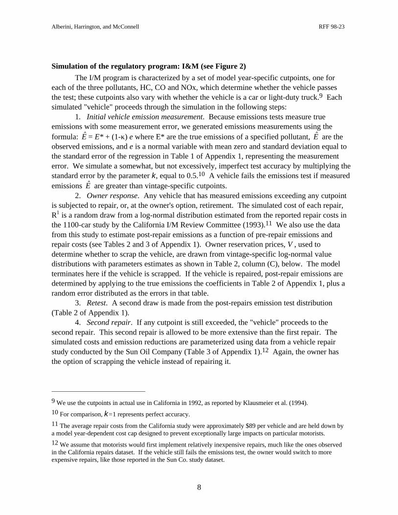
Simulation of the regulatory program: I&M (see Figure 2)

The I/M program is characterized by a set of model year-specific cutpoints, one foreach of the three pollutants, HC, CO and NOx, which determine whether the vehicle passesthe test; these cutpoints also vary with whether the vehicle is a car or light-duty truck.9 Eachsimulated "vehicle" proceeds through the simulation in the following steps:

1. Initial vehicle emission measurement. Because emissions tests measure trueemissions with some measurement error, we generated emissions measurements using theformula: $E = E* + (1-κ)⋅e where E* are the true emissions of a specified pollutant, $E are theobserved emissions, and e is a normal variable with mean zero and standard deviation equal tothe standard error of the regression in Table 1 of Appendix 1, representing the measurementerror. We simulate a somewhat, but not excessively, imperfect test accuracy by multiplying thestandard error by the parameter κ, equal to 0.5.10 A vehicle fails the emissions test if measuredemissions $E are greater than vintage-specific cutpoints.

2. Owner response. Any vehicle that has measured emissions exceeding any cutpointis subjected to repair, or, at the owner's option, retirement. The simulated cost of each repair,R1 is a random draw from a log-normal distribution estimated from the reported repair costs inthe 1100-car study by the California I/M Review Committee (1993).11 We also use the datafrom this study to estimate post-repair emissions as a function of pre-repair emissions andrepair costs (see Tables 2 and 3 of Appendix 1). Owner reservation prices, V , used todetermine whether to scrap the vehicle, are drawn from vintage-specific log-normal valuedistributions with parameters estimates as shown in Table 2, column (C), below. The modelterminates here if the vehicle is scrapped. If the vehicle is repaired, post-repair emissions aredetermined by applying to the true emissions the coefficients in Table 2 of Appendix 1, plus arandom error distributed as the errors in that table.

3. Retest. A second draw is made from the post-repairs emission test distribution(Table 2 of Appendix 1).

4. Second repair. If any cutpoint is still exceeded, the "vehicle" proceeds to thesecond repair. This second repair is allowed to be more extensive than the first repair. Thesimulated costs and emission reductions are parameterized using data from a vehicle repairstudy conducted by the Sun Oil Company (Table 3 of Appendix 1).12 Again, the owner hasthe option of scrapping the vehicle instead of repairing it.

9 We use the cutpoints in actual use in California in 1992, as reported by Klausmeier et al. (1994).

10 For comparison, κ=1 represents perfect accuracy.

11 The average repair costs from the California study were approximately $89 per vehicle and are held down bya model year-dependent cost cap designed to prevent exceptionally large impacts on particular motorists.

12 We assume that motorists would first implement relatively inexpensive repairs, much like the ones observedin the California repairs dataset. If the vehicle still fails the emissions test, the owner would switch to moreexpensive repairs, like those reported in the Sun Co. study dataset.

9

Figure 2. Driver Decisions under Different Policies

I. Pure Scrap Program

II. Scrap with Regulatory (I/M) Program

III. Scrap with Emissions Fee

emissions test

pass

fail,scrap offer = S

scrap ifS>V-R1

repair andretest

scrap ifS>V-R2

repair

pass

fail/ $450waiver

pass

Scrap offer = $S

Scrap if S>V

Scrap if S<V

emissions test

pay fee ifFee1 + R1 < Fee0

Emissonsfee levied

scrap ifS>V-(Fee1+R1 ) or if

S>V-Fee0

repair ifFee1 + R1 < Fee0

scrap ifS>V-(Fee2+R2 ) or if

S>V-Fee1

repairFee2 + R2 < Fee1

pay fee ifFee2 + R2 < Fee1


10

5. Stop. If the vehicle remains unable to pass the test after the second repair, it isallowed to be operated even though it is in violation.

Simulation of the economic incentive program: emissions fee (see Figure 2)

The emissions fee policy uses many of the same elements as the regulatory program.The main difference is in the importance of predicting the reduction in emissions, since thedecision to repair the vehicle is based on this prediction. The following steps are developed:

1. Initial vehicle emission measurement and calculation of initial fee:

( ){ }∑ −= iii BaselineEtFee ˆ,0max0

where t i is the fee rate for each pollutant, $E i the measured emission rate (which gives totalliability under the emissions fee program after it is multiplied by miles and fee rate), andBaseline the level of "free" (tax-exempt) emissions granted each vehicle, if there are any.

2. Prediction of emission reductions and estimation of post-repair fee:

{ }EstFee t E Baselinei i i1 0 10 000= ⋅ −∑max , ( ,~

)

where %E is predicted emissions using the repair cost and effectiveness from the CaliforniaI/M Review Committee study. The predicted repair is based on the regression whose resultsare reported in Table 2 of Appendix 1 -- i.e., post-repair emissions are a function of pre-repairemissions, estimated repair cost, and vehicle model year. We assume that owners have areasonable, but not perfect, ability to predict the emissions reduction attained through therepairs.13

3. Compare Fee 0 , Repair cost + EstFee1 and Owner's Value V, net of scrap value. IfFee 0 is the smallest, do nothing. If Repair cost + EstFee1 is smallest, repair. Otherwise,

scrap. "Scrap value" is replaced by the bounty offered to owners of older cars as aninducement to vehicle retirement when we consider emissions fees combined with ascrappage program.

4. Repeat 2 and 3, using the Sun Oil Co. repair cost and effectiveness (see Table 3 ofAppendix 1).

The decision rules for all three cases are summarized in the flow chart in Figure 2.

13 We simulate improvement in repair-effectiveness prediction with a parameter λ defined in the unit interval,with λ=0 representing the predictive ability shown in Table 4 and λ=1 representing perfect predictability. Forthe simulation model of this paper, λ is set to 0.5. We allow both λ and κ to vary in a related paper (Harrington,McConnell, and Alberini, 1996) in which we discuss changes in technical parameters of the model, the precisionof the emissions measurement (variations in κ) and the ability to predict repair effectiveness (variations in λ),and use the simulation model to examine the effect on emission reductions and costs of changes in the fee rates,cutpoints and other policy parameters. Harrington and Walls (1996) use a similar model to examine thedistributional implications of various in-use vehicle emission policies.


11

4. THE DISTRIBUTION OF VEHICLE VALUES

A critical component of the decision to scrap is the value of the current vehicle, andvehicle values vary with the condition and quality of the vehicle. The simulations, asdescribed above require a distribution of vehicle values across the fleet. In his study ofscrappage Hahn (1995) used blue book values for each make and model year, distinguishingbetween two categories of vehicles, those in good condition and those in fair condition. Thismethod neglects the range of differences that are likely to occur between individual vehiclesand the group average. Our analysis attempts to address this problem by estimating the entiredistribution of vehicle values. However, because data are not available documentingindividual vehicle condition and value for California which serves as the empirical bases forthe simulated fleet, we draw on available evidence from a survey of old car owners conductedas part of the Delaware Vehicle Retirement Program of 1992, and then "transfer" thesevintage-specific distributions to the simulated California fleet.

The Delaware dataset is comprised of a random sample of older (pre-1980) vehicles inDelaware, some of which were scrapped in the Delaware Vehicle Retirement Program, andsome of which owners elected not to scrap. The data includes information about both vehiclecharacteristics and owner characteristics, and is described in detail in Appendix 2. Using thedata, we estimate a model that relates the price at which the owner would be willing to scraphis vehicle (willingness-to-accept (WTA)) -- our best measure of the value of a vehicle to itsowner -- to condition, use and repair information. The dependent variable in our regressionmodel is, therefore, WTA. The estimated coefficients in the WTA model are used todetermine the distribution of vehicle values used in the simulation model.

The theoretical model described in Section 2 above of vehicle scrappage andownership implies that the value of a vehicle, reflects the present and future benefits andcosts of driving it. We assume that the benefits (B in our theoretical equations) depend onindividual and household characteristics, such as household income, age of the owner, size ofthe family, how many cars the household owns relative to the number of household membersor licensed drivers, and the need to use the car for work-related purposes. Other variables,such as the age of the vehicle, its condition, past repairs, the total miles on the vehicles, themiles driven in the most recent period, and factors describing emissions, such as the vehicle'swaiver status, proxy the cost of maintenance and repairs (C in our theoretical equation).14

Among car characteristics, we expect higher odometer mileage, older age and poorcondition to decrease the value of the car. Waiver status may also decrease the value of thecar, whereas the effect of past maintenance and repairs is uncertain a priori: high maintenanceexpenditures in the past may imply that this vehicle has been taken good care of, but may alsosignal a poor quality car.

14 Note that all of these variables are predetermined (they are the results of decisions and repair expendituresundertaken in the past, but not the object of current decisions) or are outside of the owner's control (such as theage of the vehicle). This ensures that the regressors in our econometric model of WTA are not simultaneouslydetermined with the dependent variable, WTA.


12

Econometric Results

We initially ran regressions that included both the vehicle characteristics (affectingcosts) as well as individual/household characteristics, which are assumed to be the maindeterminants of the benefits of owning the vehicle. However, individual and householdcharacteristics were never significant in the models of WTA that included both these andvehicle attributes,15 so we report results for those regressions that only include determinantsof costs among the regressors.

Table 1. WTA model: Dependent variable: log WTA

(T statistics in parentheses)

Independent variable (A) (B) (C)

Intercept 12.6836(9.057)

2.9667(2.353)

7.4719(25.311)

Age of car in yrs -0.0540(-1.734)

0.0078(0.299)

-0.0333(-1.957)

Log miles -0.3491(-2.895)

Log miles driven, past yr -0.1279(-1.700)

-0.0363(-0.665)

Condition dummy -0.8264(-6.013)

-0.7683(-7.926)

Log blue book value 0.5847(5.506)

Log of $ spent on repairs 0.0999(0.987)

0.0915(1.186)

I/M waiver status -0.1000(-0.706)

0.0252(0.216)

Num. Veh owned by hh 0.0068(0.199)

stand devn of error 1.1729(14.833)

1.0247(17.313)

1.2048(20.301)

sample size 344 404 632

log L -216.33 -267.64 -458.02

Table 1 shows the results for various specifications of the econometric model.Column (A) includes age and condition of the vehicle, recent and cumulative miles driven,recent maintenance expenditure and waiver status among the independent variables. Asshown in Column (A), as we expected, age tends to depress the value of the vehicle (the

15 These results are consistent with those reported by Morey (1996), who analyzes willingness to accept datafrom the Total Petroleum scrappage program. In our case the result may be due to the collinearity betweenindividual characteristics and vehicle attributes/expenditures.


13

coefficient of age being negative and significant at the 10 percent level), but the effect of ageis dominated by that of odometer miles (which tend to be correlated with age, and have anegative and highly significant coefficient) and condition of the car. The miles driven in theprevious year also tends to correlate negatively with WTA (the coefficient being significant atthe 10 percent level). Waiver status does not seem to affect the value of the car. Thecoefficient of past maintenance is positive, but not significant at the conventional levels.

In Column (B) we eliminate odometer reading and include blue book value at the timeof the first survey.16 Blue book value and condition are two of the strongest predictors ofWTA. This suggests that the owner-assessed value of the vehicle tends to follow the marketaverage for vehicles of that model year, the difference relative to this average being explainedby the condition of the vehicle "for its age." In the span of time covered by our surveys(about two years) the present condition of the vehicle is sufficient to explain the decline invalue relative to the initial-survey blue book value: the miles recently driven and age have noadditional explanatory power, suggesting that miles and age are correlated with condition.

These regressions confirm our priors on the relationship between use, condition andvalue of a vehicle, and indicate that value does systematically decline with the age of thevehicle. Column (C) of Table 1 isolates the effect of vintage alone, which is we use for thesimulations discussed in the remainder of the paper. Age is a significant predictor of WTA,its coefficient being negative and significant at exactly the 5 percent level.17 When the meanand variance of log WTA within each model year are estimated, the dispersion around thevintage-specific mean increases slightly with age. Because we have only age of the Californiafleet, we use this simple equation to predict vehicle values be used in the simulation.

5. RESULTS OF THE SIMULATION MODEL

To illustrate the interaction of scrappage bounties with other regulatory policies for in-use emissions we use the empirical results on vehicle value as inputs to the simulation modeldeveloped above. Owners of the 1,000 car fleet make decisions to either keep, repair or scraptheir vehicles under different policy regimes, using the simulation process described inSection 3 above. Here, we examine the regulatory policy (I/M) and emission fee policies bothwith and without the option to scrap an old vehicle. The I/M program examined has cutpointsset at a level of about twice the mean emission rate of all vehicles, a level that is lenientrelative to the new-car emission standards, but probably is representative of the "transitional"cutpoints used in the first year of some Enhanced I/M programs. We compare these policiesto a pure scrap program. The various policies can be evaluated in a number of different ways

16 Blue book value is predicted from age and odometer reading. We include current age and miles driven mostrecently to proxy for what the blue book value would be at the time of the second and third round surveys.

17 We also ran regressions in which WTA at the time of the previous round of survey was included among theindependent variables. We found that today's value is strongly correlated with the vehicle value reported by theowner in the immediately preceding round of surveys, all other variables (miles driven between the two surveys,present condition of the car, etc.) offering no additional explanatory power.


14

including the impact on scrappage and repair, on emissions reduction potential, on cost-effectiveness, and on net economic benefits.

We examine only the results of the first year of the program, After the first year,presumably, fewer vehicles would be scrapped because the worst vehicles would have beenremoved. We assume the remaining life of a vehicle sent to the scrapyard by a scrap or I/Mpolicy would have been one year in the absence of a policy.18 We also assume that repairsrequired to bring the vehicle in compliance with the I/M program are effective for one year:Should a vehicle be scrapped, its replacement is assumed to be the average vehicle in the fleet.

We first examine the results of the regulatory program (I/M) and emissions fees onscrap and repair rates. Figures 3a and 3b show the results of including a scrap program withan I&M program and an emissions fee. First, with no structured old car scrap program(bounty equal to $0), about 2 percent of the fleet is scrapped due to both average fleetturnover and the presence of the I/M program and its required repairs. With the emissions feepolicy (no baseline) set at the level of marginal damages ($3,000 per ton of hydrocarbons and$10,000 per ton of NOx)19, with no scrap offer, about 7 percent of the fleet is scrapped. Inboth cases, when a scrap program is introduced, increases in the scrap offer cause drivers toelect to scrap instead of repair. Those cars that are scrapped will be the ones that have thehighest expected repair cost relative to the driver's valuation of the car.

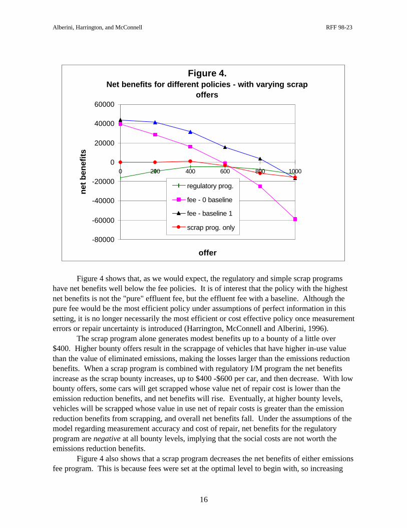
Figure 4 addresses the broader issue of the net benefits under different policies as thescrap offer varies from 0 to $1,000. Benefits are calculated as the emissions reductions undereach policy times a constant marginal damage function. We use marginal damages estimatesfrom Small and Kazimi (1995) of $3,000 per ton of hydrocarbons and $10,000 per ton ofnitrogen oxides. We examine cases where the fees vary between half and twice the marginaldamages, but the results reported here refer to the case where the fees equal the assumedmarginal damages.20

18 Both EPA guidelines (1993) and Hahn (1995) assume that the remaining life would have been 3 years. In ourearlier work we find, based on the owner planned vehicle retirement, that the average remaining life of a vehicleparticipating in a scrap program that offers up to $1000 per car is generally well below 3 years.

19 The damages from vehicle emissions include the increased morbidity from ozone formed by HC and NOxemissions and the increased mortality caused by some types of particulates including some NOx particulates.Small and Kazimi (1995) find that the mortality effects from nitrogen oxides are about 3 times higher than thedamages from hydrocarbons. This estimate, especially for NOx emissions, is high relative to other estimates ofair pollution damages (see Krupnick and Portney, 1991).

20 The costs of each program are calculated as the repair cost, plus the cost of scrapping cars early (the value ofthe cars that get scrapped). To keep costs comparable across policies, we do not count the fee payment as part ofthe social cost in the case of the emissions fees, assuming that taxes will be reduced by an equal amountelsewhere. Similarly, with the scrap program bounty, we assume that taxes must be raised elsewhere to raise themoney to make the bounty offers, so there is simply a redistribution of funds. The costs and subsidies are,however, very real to drivers. Finally, we do not include the testing costs under the regulatory or fee policy,because we assume these costs would be the same under either policy. Testing costs depend more than anythingelse on test frequency, which is beyond the scope of our one-year comparison.


15

Figure 3a. Regulatory Program

0

50

100

150

200

250

300

350

0 200 400 600 800 1000

scrap offer

nu

mb

er o

f ve

hic

les

no. cars repaired

no. cars scrapped

Figure 3b. Emissions Fee Program, Zero Baseline

0

50

100

150

200

250

300

350

400

0 200 400 600 800 1000

scrap offer

nu

mb

er o

f ca

rs

no. of cars repaired

no. of cars scrapped


16

Figure 4.Net benefits for different policies - with varying scrap

offers

-80000

-60000

-40000

-20000

0

20000

40000

60000

0 200 400 600 800 1000

offer

net

ben

efit

s

regulatory prog.

fee - 0 baseline

fee - baseline 1

scrap prog. only

Figure 4 shows that, as we would expect, the regulatory and simple scrap programshave net benefits well below the fee policies. It is of interest that the policy with the highestnet benefits is not the "pure" effluent fee, but the effluent fee with a baseline. Although thepure fee would be the most efficient policy under assumptions of perfect information in thissetting, it is no longer necessarily the most efficient or cost effective policy once measurementerrors or repair uncertainty is introduced (Harrington, McConnell and Alberini, 1996).

The scrap program alone generates modest benefits up to a bounty of a little over$400. Higher bounty offers result in the scrappage of vehicles that have higher in-use valuethan the value of eliminated emissions, making the losses larger than the emissions reductionbenefits. When a scrap program is combined with regulatory I/M program the net benefitsincrease as the scrap bounty increases, up to $400 -$600 per car, and then decrease. With lowbounty offers, some cars will get scrapped whose value net of repair cost is lower than theemission reduction benefits, and net benefits will rise. Eventually, at higher bounty levels,vehicles will be scrapped whose value in use net of repair costs is greater than the emissionreduction benefits from scrapping, and overall net benefits fall. Under the assumptions of themodel regarding measurement accuracy and cost of repair, net benefits for the regulatoryprogram are negative at all bounty levels, implying that the social costs are not worth theemissions reduction benefits.

Figure 4 also shows that a scrap program decreases the net benefits of either emissionsfee program. This is because fees were set at the optimal level to begin with, so increasing


17

the bounty for old cars will cause less than optimal decisions to be made -- some vehicles willbe scrapped whose value in use exceeds the emission reduction benefits. Generally, however,Figure 4 shows that emissions fee policies prove superior to the other alternatives considered,especially for the variant without exempt emissions.

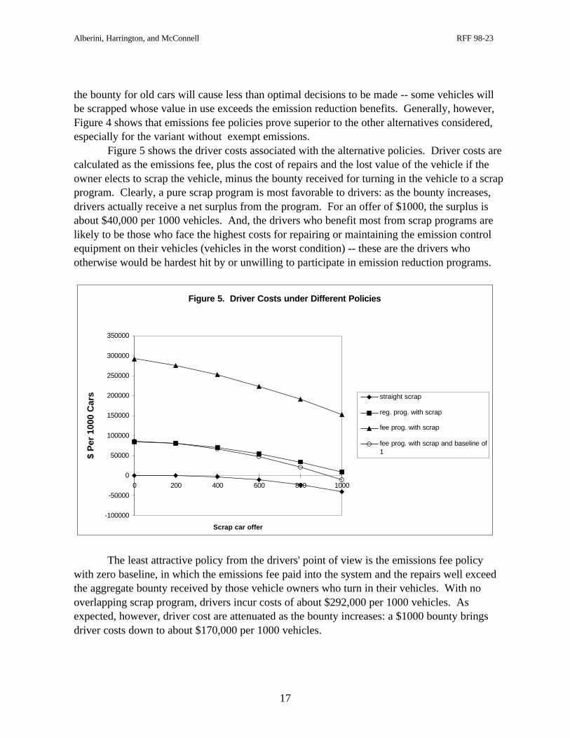
Figure 5 shows the driver costs associated with the alternative policies. Driver costs arecalculated as the emissions fee, plus the cost of repairs and the lost value of the vehicle if theowner elects to scrap the vehicle, minus the bounty received for turning in the vehicle to a scrapprogram. Clearly, a pure scrap program is most favorable to drivers: as the bounty increases,drivers actually receive a net surplus from the program. For an offer of $1000, the surplus isabout $40,000 per 1000 vehicles. And, the drivers who benefit most from scrap programs arelikely to be those who face the highest costs for repairing or maintaining the emission controlequipment on their vehicles (vehicles in the worst condition) -- these are the drivers whootherwise would be hardest hit by or unwilling to participate in emission reduction programs.

Figure 5. Driver Costs under Different Policies

-100000

-50000

0

50000

100000

150000

200000

250000

300000

350000

0 200 400 600 800 1000

Scrap car offer

$ P

er 1

000

Car

s straight scrap

reg. prog. with scrap

fee prog. with scrap

fee prog. with scrap and baseline of1

The least attractive policy from the drivers' point of view is the emissions fee policywith zero baseline, in which the emissions fee paid into the system and the repairs well exceedthe aggregate bounty received by those vehicle owners who turn in their vehicles. With nooverlapping scrap program, drivers incur costs of about $292,000 per 1000 vehicles. Asexpected, however, driver cost are attenuated as the bounty increases: a $1000 bounty bringsdriver costs down to about $170,000 per 1000 vehicles.


18

Figure 6 shows the total social cost functions for reducing emissions under thealternative policies, for different scrappage offer prices. Each point on the line for I/M andemissions fees represents a different offer price, from 0 to $1,000 in $200 increments. Theline for the pure scrap program is based on bounty levels ranging from $300 to $1000 in $100increments. Emissions reduced are given in terms of weighted tons reduced, where tons areweighted according to the marginal damages from HC and NOx (NOx emissions are weighted3 times higher than HC).21

F igure 6 . S o c ia l c o s ts a n d to n s re d u c e d

0

50000

100000

150000

200000

0 10 20 30 40 50

W e i g h t e d t o n s r e d u c e d

Regulatory programFee, baseline=0Fee, baseline=1Pure scrap program, bounty=$300-$1000

For all of the policies we examine, the emissions reductions do increase with thebounty offered by the companion scrap program. The stand alone scrappage program isrelatively low cost, but provides relatively few emissions reductions, a finding that confirmsthe evidence from other analyses (Alberini et al., 1994). Based on social costs, the costeffectiveness of a pure scrappage program (shown in Figure 7) is about $1900 per weighted

21 For comparison, Hahn (1995) assigns weights of 1 and 1.8 to HC and NOx emissions, respectively.


19

ton of the pollutants when the bounty is $300. Cost-effectiveness deteriorates as the scrapoffer increases: at $1000 scrap price, the cost effectiveness is $4700 per weighted ton. Thetotal weighted tons of pollutants reduced range from only 2.3 (at $300) to about 12 (at $1000).

Figure 7Cost per ton of pollutant removed

0

500

1000

1500

2000

2500

3000

3500

4000

4500

5000

0 200 400 600 800 1000

Offer (in $)

$

scrap alone

I/M

fee 0

fee 1

The regulatory program, on the other hand, attains a much higher level of emissionsreductions (20 to 35 tons), albeit at a higher cost. Its cost-effectiveness, however, is relativelyinsensitive to the scrap offer, since it is at $4200 per weighted ton in the absence of a formalscrap program, about $4070 per weighted ton at a bounty of $400, and about $4500 at a scrapoffer of $1000. These figures are relatively close to the cost-effectiveness calculations inHahn (1995).

Of the two emissions fee programs, the one with exempt emissions has emissionsreduction potential comparable to that of the regulatory I/M program (21 to 32 tons), but ismuch less costly. Its cost-effectiveness is about $1100 per weighted ton with no scrap offer,and worsens to about $3700 when the scrap offer is $1000. Adding a scrap program withsuccessively higher scrap offers raises cost more quickly with the fee policies than with theI&M policy. This is because the low-valued high emitting cars have already been scrappedunder an emissions fee policy, so scrapping additional cars will bring in higher valued cars.

The greatest emissions reduction potential comes from the fee program with noemissions exemption, which can eliminate up to 39 tons of pollutants. Its cost-effectivenessranges from $1800 to $4700 per ton removed, a performance that is inferior to that of theemissions fee without exemption but better than that of the I/M program for most of thebounty levels we examined.


20

6. CONCLUSIONS

We have included a model of the owner's decision to scrap or repair a vehicle in asimulation model of a vehicle fleet. This model has been used to evaluate the role ofscrappage programs as an independent policy or in combination with an I/M or fee policy. Acritical part of the model is the owner's valuation of his/her car. We examined the factorsaffecting owners valuations of their old vehicles using a unique longitudinal dataset.Willingness to accept is well predicted by the owner's valuation in last period, and on themileage and condition of the car. Other inputs into the simulation models are the estimateddistributions of emissions in the fleet, and the link between emissions reductions and the costof repairs. We use empirical estimates of both of these in the simulations.

The simulation model is used to examine the role of scrap policies alone andcombined with other policies for reducing emissions, such as current state I/M program andproposed emissions fees, and the welfare implications of combining such programs. Themodel assumes that of all possible options (repairing the car, scrapping the vehicle or turningit in to an old car scrap program, paying the emissions fee without repairing the vehicle) theowner will choose the one with the least cost.

We find that old car scrap programs may increase net welfare under a regulatoryprogram like I/M in practice today, but that a stand alone scrap program is unlikely to providevery much in the way of emission reductions. Our simulations suggest that emissions fees area cost-effective way to reduce emissions, and that their technical and political feasibilityshould be explored. Their cost-effectiveness is highest in the absence of an overlappingscrappage program, and ranges between $1100 and $1800 per ton of pollutants removed,depending on whether the policy allows for exempt emissions. Cost-effectiveness worsens --while remaining still comparatively better than that afforded by the regulatory approach -- asa bounty is introduced, which considerably lessens driver costs.


21

APPENDIX 1. DESCRIPTION OF THE SIMULATION MODEL

Emissions in the California fleet

We fit joint log normal distributions to vintage-specific emissions rates of HC and COas measured by remote sensing of over 90,000 vehicles in the Los Angeles region in 1991.22,

23 Both HC and CO are expressed in grams per mile.Nitrogen oxides readings are taken from a sample of 7234 vehicles given IM240 tests

at EPA's Hammond, Indiana, test facility. Within each model year, NOx emissions arereasonably approximated by a log normal variable. When we artificially generate the data forour simulation exercise, we assume that NOx emissions rates are independent of HC and COemissions rates.

Reliability of the BAR-90 test

Motorists and the state agency in California rely on the so-called BAR-90 testprocedure to determine whether a vehicle is in compliance with the prescribed emissionsrates. One important issue is whether this test procedure provides a truthful picture ofvehicles' emissions. To answer this question, we use data collected by the California I/MReview Committee "undercover car" study (1993) and estimate statistical models ofemissions measurement (as opposed to true emissions). It is measured emissions that formthe basis for the owner decision to repair or scrap the vehicle.

The BAR-90 is a two-speed test that includes, in addition to the idle test, a test ofemissions at an engine speed of 2500 RPM. It is usually regarded as inferior to testsinvolving the use of a dynamometer and the operation of a vehicle over many differentdriving modes, including acceleration, deceleration, stop and start. The Federal TestProcedure (FTP) is one such test and is currently considered by regulators and the automotiveindustry as the best method to produce an estimate of actual vehicle emissions.24

In an effort to assess the performance of the Smog Check program, the California I/MReview Committee study recruited a large number of vehicles in use which were given an

22 Remote sensing is a technology combining roadside monitors that send infrared beams from one side of theroad to a detector on the other side, measuring a vehicle's emissions, with a video camera that obtains aphotograph or electronic identification of the license plate. See Stedman, et al. (1994), for a discussion ofremote sensing technology and the California data used in this study.

23 We are here implicitly assuming that the distribution of emissions rates in the Los Angeles basin isrepresentative of emissions rates in the whole state.

24 The FTP is the test procedure currently used to certify new automobiles for compliance with the emissionsrequirements of the 1977 Clean Air Act. The test takes about an hour to complete and is quite expensive toperform (about $1000 per test). Enhanced inspection and maintenance programs generally rely on the IM240, afour-minute and much less expensive variant of the FTP. Recently, however, the FTP test has been criticized fornot accurately reflecting true driving behavior and accompanying on-road emissions. Specifically, the FTPallegedly underrepresents high acceleration episodes (Ross et al., 1995). There is only limited empiricalevidence confirming that the results of IM240 tests closely resemble those of the FTP tests.


22

initial FTP test. Those vehicles that failed the FTP were sent out to a sample of Smog Checkstations in Southern California as if they were ordinary cars out to get their required SmogCheck certificates. These "undercover" cars were given emission tests by the (presumably)unsuspecting Smog Check stations and, if failing, were repaired and retested. The cars werethen given a post-repair FTP test. Of the 1100 vehicles originally included in the program, wework with a data set of 681 vehicles for which repairs were attempted and a second FTPcompleted.

The performance of the idle test was evaluated by regressing the FTP test results(before repairs) for a specific pollutant on the BAR-90 idle test results:

FTP IdleHC IdleCO= + + +α α α ε0 1 2 . (A1.1)

where FTP refers to the FTP test emissions for HC, CO and NOx, in grams per mile, IdleHCthe HC idle test results in ppm and IdleCO the CO idle test results in percent CO. Becausethe idle test results are expressed in parts per million and percent, respectively, and the FTPtest results are expressed in grams per mile, the regression coefficients are interpreted asconversion factors from one unit of measurement to the other.25

Results, with standard errors in parentheses, are given in Table A1 below. As shown,the idle test results are completely ineffective at explaining FTP results for NOx and explainabout a third of the variation in emissions of HC and CO. The most important parameters arethe standard errors of the regressions, for these are used to generate the random normaldeviates that serve as emissions measurement errors in our simulation model.

Table A1. Ability of the Idle Test to Predict FTP Emissions

Dependent Variable (grams/ mile)

FTP HC FTP CO FTP NOx

Constant 1.305

(0.314)

25.36

(1.90)

2.09

(0.074)

Idle HC

(ppm)

0.00890

(0.00054)

0.0070

(0.0032)

0.37e-3

(0.12e-3)

Idle CO

(percent)

0.279

(0.090)

9.93

(0.54)

-0.042

(0.021)

R-square 0.34 0.37 0.01

Standard error 5.86 35.52 1.38

N 669 669 669

Source: California I/M Review Committee, 1993. Standard errors in parentheses.

25 Only HC and CO idle test emissions rates are included in the right-hand side of equation (4), as NOx rates arenot measured by the BAR-90.


23

Cost-effectiveness of Repairs

Recent results suggest that vehicle emissions repair is not nearly as effective as hadpreviously been assumed. In 1992 the EPA, in assessing the cost-effectiveness of theproposed Enhanced I/M regulation (EPA, 1992), assumed emission repairs to cost an averageof $120 each and to be relatively effective at reducing emissions.

However, three recent studies indicate that vehicle emission repairs are much lesssuccessful and more expensive than assumed by the EPA. One of those studies produced the681-car dataset described in the preceding section (California I/M Review Committee, 1993),which indicated that the average cost was low (less than $90 per vehicle), probably a result ofwaiver limits that restricted the amount spent on each vehicle. The average emissionsreduction was also low: 25 percent for HC, 21 percent for CO, and 8 percent for NOx.Emissions reductions were also quite variable across vehicles, with nearly half the carsshowing higher emissions after repair than before. Emissions reductions were not at allrelated to cost.

In two other recent repair studies the repairs were more effective, but far moreexpensive than assumed by the EPA. Both studies were conducted by oil companiessearching for mobile source reductions to use as emissions offsets for stationary sourceemissions. In 1993 Sun Oil Company (Cebula, 1994) used remote sensing to identify gross-emitting vehicles owned by their employees as they left company parking lots in Philadelphia.Sun offered to repair these vehicles at its expense, and spent up to $450 on each vehicle.After an average expenditure of $338, the emissions reductions for HC, CO and NOx were 68percent, 75 percent and 9 percent, respectively. While quite an improvement over theCalifornia results, the emissions reductions attained in the Sun program are still a far cry fromthe EPA assumptions. Moreover, fully 40 percent of the vehicles were not brought intocompliance even after an expenditure of $450.

Another study was done by Total Petroleum in Denver. This was a combined scrap-repair study, in which gross-emitting vehicles were identified by several different means.This study found that emissions of HC and CO were reduced by about a third after an averageexpenditure of nearly $400.

Ideally, we would like to estimate a repair model that gives the emissions reductionsfollowing from making certain kinds of repairs.26 Unfortunately, we have not been able tolocate data that allow us to estimate the effectiveness of specific repairs. The three studiesearlier discussed record initial and post-repairs emissions, and the cost of the repairs, but notrepair type. Using the data from the California I/M Review Committee and the Sun Oil Co.studies we fit the following equation of repair effectiveness: 26 Predictability of the emissions reductions associated with a given level of repair costs would be extremelyuseful in an I/M program, as mechanics would be able to select the combination of repairs that brings the vehicleinto compliance with the emissions standards at the least cost. Repair predictability would be even more usefulin an emissions fee program, since the mechanic could decide on the package of repairs that maximizes theexpected net benefit of repair to the motorist -- that is, the expected reduction in emissions fees paid less the costof repair. This choice can include the possibility of making no repairs at all if it is less costly to pay the fee.


24

E E Age Costj i i1

00

1 2= + + + +∑β β γ γ η (A1.2)

where i j HC CO NOx, , ,= are the pollutants of interest; E E0 1, refer to emissions before andafter repair, respectively; Age is the vehicle age in years; Cost is the reported repair cost. Thevariable η is the disturbance term, which is assumed normal.

The results for California (Table A2) show that by far the most significant predictor ofpost-repair emissions of a pollutant are the pre-repair emissions of that same pollutant. Thecoefficients can be interpreted as the marginal effectiveness of repair at removing pollutantsfrom vehicle emissions. The coefficient of 0.36 for HC, for example, means that repair in theCalifornia program removed 64 percent of the incremental HC emissions. The effects of otherpollutants are not consistently related to post-repair emissions. Cost is significant for CO andNOx and has the correct sign for all three pollutants, but in all cases the numerical magnitudesare so small that cost has no practical importance. (For example, an expenditure of $100 reducesexpected HC emissions by 0.1 grams per mile.) The coefficient of Age (not reported forconsistency with Table 5) is positive and significant in the CO and HC equations, the positive signsuggesting either that older vehicles are more difficult to repair or that what must be consideredthe emission level for a fully repaired vehicle increases slowly with vehicle age. On average, ayear of age increases post-repair emissions by 0.1 g/mi. for HC and 1 g/mi. for CO.27

Table A2. Predicting Repair Effectiveness: California I/M Review

Dependent variable (grams per mile)

HC CO NOx

Constant 0.041 5.30 0.14(0.25) (1.40) (0.048)

HC0 0.36 0.53 -0.0025

(0.027) (0.15) (0.0051)CO0 0.026 0.62 0.0027

(0.0045) (0.024) (0.00084)NOx0 0.32 0.60 0.73

(0.13) (0.72) (0.025)Cost -0.00084 -0.011 -0.00027

(0.00064) (0.0034) (0.00012)Std. error 2.87 15.54 0.54R-square 0.34 0.59 0.57n 669 669 669

Standard errors in parentheses.

27 Table 4 reports the results of a regression in which both the dependent variable and the independent variablesare untransformed. We experimented with double-log, semi-log and quadratic models, as well as models forpercentage changes in emissions, and found that the results were qualitatively similar: the cost of repairs is astatistically significant predictor of post-repair emissions, but has virtually no practical importance.


25

Similar regressions run on the Sun Co. data (Table A3) show even higher pollutantremoval efficiencies, owing most likely to the greater repair expenditure. The age of thevehicle was insignificant and has been omitted from the model in the table.

Table A3. Predicting Repair Effectiveness: Sun Oil Company

Dependent variable (grams per mile)

HC CO NOx

Constant 0.36 2.48 1.04(0.28) (3.45) (0.24)

HC0 0.098 0.16 0.10

(0.026) (0.32) (0.023)CO0 -0.0036 -0.00051 -0.0041

(0.0015) (0.018) (0.0013)NOx0 0.0055 -0.26 0.011

(0.020) (0.24) (0.017)Cost 0.0013 0.023 0.00017

(0.00075) (0.009) (0.00066)R-square 0.11 0.05 0.12Std. error 1.20 14.58 1.05n 151 151 151

Standard errors in parentheses.

In the simulation model described in the next section we use the linear model becauseits coefficients are easier to interpret and because we are more interested in prediction of thevalue of the dependent variable than in the coefficients per se. Specifically, the results fromthe California I/M Review study are used to generate the repair size and emissions reductionsfollowing the first round of repairs; the results from the Sun Co. study are used to generatedthe repairs and emissions reductions after the second round the repairs, if the vehicle fails thesecond test.


26

APPENDIX 2. DATA SUMMARY: DELAWARE VEHICLE RETIREMENT PROGRAM

The Data

We obtained owner-assessed values for relatively old vehicles in the course ofinterviews of vehicle owners conducted in association with the Delaware Vehicle RetirementProgram (DVRP; see Alberini et al., 1994). The DVRP targeted approximately 4200 ownersof pre-1980 vehicles, who were offered $500 for their vehicles. The targeted owners receivedletters that spelled out the nature of the program, the bounty level and asked interested ownersto call a toll-free number in order to make arrangements for scrappage.

One-hundred twenty-five vehicles were purchased, and 121 of the owners of thosevehicles were interviewed at the scrapyard. A total of 365 non-participants (owners of pre-1980vehicles who were sent letters soliciting participation in the program, but had chosen not toparticipate) were surveyed over the telephone, whereas the 48 "waitlisted" owners (owners whoindicated they wished to participate, but had replied to the DVRP letters only after the goal of125 vehicles had already been attained) were not interviewed in this first round of surveys.

Both participants and non-participants were asked similar questions. Specifically, weverified the information on make and model year, asked whether the car had been purchasednew or used, inquired about the odometer reading, the miles driven in the previous year, thecurrent use of the vehicles for commuting and non-commuting work-related purposes anderrands, the present condition of the car and the maintenance expenditures in the previousyear as well as those planned for the next year.

In addition, we asked how much longer the owner planned to keep the vehicle, andhow he or she was planning to dispose of it at that time (by selling, trading or scrapping it).One of the most important questions elicited an estimate of the car value to the owner.28 Thesurvey ended with questions about the household's economic circumstances anddemographics.

About a year later, we once again contacted over the telephone the non-participantswho still had their pre-1980 vehicle and administered a survey questionnaire that was virtuallyidentical to that in our first round of surveys. In addition, we contacted and interviewed most(42) of the "waitlisted" owners and interviewed them over the telephone about the currentvalue of the vehicle and the value of the vehicle at the time of the DVRP letters.

Finally, another year later we re-contacted all of those non-participants and"waitlisted" owners who had reported owning the car at the time of the second round ofsurveys and repeated the standard version of our questionnaire.

28 Most respondent provided responses that we interpret as point estimates of their willingness to accept (WTA)for their vehicle. A few indicated that their WTA figure was greater than $1000, but did not specify a pointvalue. We developed special statistical models to accommodate for these responses.


27

Econometric Specifications

The three round of surveys enabled us to develop a unique longitudinal dataset thatincludes participants, non-participants who still owned their pre-1980 vehicle at the time ofthe first round of surveys, and "waitlisted" owners who still owned their pre-1980 vehiclewhen first surveyed. Non-participating and waitlisted owners provide, at regular intervalsof one year, information on the most recent condition, use, value and planned ownership fortheir car.29

Formally, the model for willingness to accept is:

logWTA xit it it= +β ε (A2.1)

where i indexes the individual (i=1, 2, ..., n), t indexes the round of surveys (t=1, …, Ti ,where Ti may be equal to one, two or three, depending on the fate of the respondent's

vehicle), x includes all exogenous variables thought to influence WTA (individual or vehiclecharacteristics), and ε it is a normally distributed error term.30 The error terms are assumedserially uncorrelated (within one owner) and independent across owners: Cov(ε it ,ε js ) is zero

for t≠s and all i's and j's.The nature of some of the observations on the value of a vehicle prevents us from

using least squares when estimating our models of willingness to pay. We resort to maximumlikelihood techniques to accommodate those respondents who -- in one or more rounds ofsurveys -- declined to participate in the scrappage program at $1000 but never reported theirexact WTA value. The log likelihood function is:

log L= ( ) log (log ; , , ) loglog

11000

11

− ⋅ + ⋅ −

==∑∑ I WTA x I

xit it it it

it

t

T

i

n i

φ β σβ

σ σΦ (A2.2)

where φ(•) and Φ(•) denote the standard normal pdf and cdf, respectively; σ is the standarddeviation of the error term, and Iit is an indicator that takes on a value of one for those

respondent who would not have participated in the program for $1000, but do not report theirexact WTA value, and zero for all others.

A description of the variables used in our regressions is provided in Table A2.1.

29 Since owners drop out of our dataset as soon as it is ascertained that they do not hold their vehicles anylonger, we have a minimum of one and a maximum of three observations per owner in the dataset. Thoseowners who still had their cars at the time of the most recent round of surveys contribute three observations.

30 We choose log WTA as our dependent variable because previous work with the data from the first-roundsurveys suggests that WTA is reasonably approximated by a log normal distribution (Alberini, Harrington andMcConnell, 1995).


28

Table A2.1. Description of Variables from the DVRP Surveys

Variable Description mean std devn min max #valid

WTA exact WTA value 1535.58 2791.27 100 20000 506

age2_ye age of the car in years 17.13 2.95 13.5 32 848

miles odometer miles 126,060 61,415.15 1000 430,467 457

pastyr miles driven in the past year 4343.92 3504.57 1000 12,000 543

wvalue Blue Book Value at time of first survey 1021.83 1046.61 100 9850 522

cond 1 if vehicle is in fair/poor condition;

0 if in excellent/good condition

0.55 0.50 0 1 861

spent how much money was spent to keep the carrunning in the past year

217.91 137.18 100 600 537

spend how much money is to be spent to keep thecar running another year

187.52 143.66 100 600 537

income household income 36,663.75 19,985.50 10,000 75,000 571

owned number of vehicles owned by the household 2.77 1.42 0 16 805

liscdriv number of licensed drivers in the household 2.09 0.90 0 6 856

waiver 1 if the vehicle has been granted waiverstatus; 0 otherwise

0.34 0.47 0 1 861

age years of age of the owner 49.48 15.95 18 92 807

Other variables used in the WTA regressions: lmiles = log odometer miles; lpastyr = log miles driven in the past year;lwvalue = log Blue Book value; lspent = log(spent); lincome = log household income.


29

REFERENCES

Alberini, Anna, David Edelstein, Winston Harrington, and Virginia McConnell. 1994.Reducing Emissions from Old Cars: The Economics of the Delaware Vehicle RetirementProgram, Discussion Paper QE94-27, Resources for the Future, Washington, D.C., April.

Alberini, Anna, Winston Harrington, and Virginia McConnell. 1995. "Determinants ofParticipation in Accelerated Vehicle Retirement Programs", The Rand Journal ofEconomics, vol. 26, no. 1, Spring.

Alberini, Anna, Winston Harrington, and Virginia McConnell. 1996. "Estimating anEmissions Supply Function from Accelerated Vehicle Retirement Programs," The Reviewof Economics and Statistics, 78, pp. 251-265.

American Automobile Manufacturers Association (AAMA). 1995. AAMA Motor VehicleFacts & Figures (Detroit, Mich.: AAMA).

California I/M Review Committee. 1993. "Evaluation of the California Smog CheckProgram and Recommendations for Program Improvements," Fourth Annual Report tothe Legislature, February 16.

Cebula, Francis J. 1994. "Report on the Sunoco Emissions Systems Repair Program," SunOil Company, Philadelphia, Pennsylvania.

Dickson, Edmund L., R. C. Henning, and W. R. Oliver. 1991. "Evaluation of VehicleEmissions from the UNOCAL SCRAP Program," Radian Corporation, Sacramento,California, June.

Energy and Environmental Analysis, Inc. (EEA). 1994. "Draft User's Guide for EFEEVersion 1.0, An Emissions-Based Fee Model," prepared for the U.S. EnvironmentalProtection Agency, Arlington, Virginia, March.

Gruenspecht, Howard K. 1982. "Differentiated Regulation: A Theory with Applications toAutomobile Emissions Control," Ph.D. dissertation, Yale University.

Hahn, Robert W. 1995. "An Economic Analysis of Scrappage," The RAND Journal ofEconomics, vol. 26, no. 2, pp. 222-242.

Harrington, Winston, Virginia McConnell, and Anna Alberini. 1996. "Economic IncentivesUnder Uncertainty: The Case of Emissions Fees," Discussion Paper QE96-32, Resourcesfor the Future, Washington, D.C., August.

Harrington, Winston, and Margaret Walls. 1996. "Controlling Vehicle Emissions: TheEfficiency and Equity of Taxes versus Standards," paper presented at the AEA annualmeetings, San Francisco, January.

Illinois Environmental Protection Agency. 1993. "Pilot Project for Vehicle Scrapping inIllinois," Springfield, Illinois, May.

Kazimi, Camilla. 1997. "Evaluating the Environmental Impact of Alternative FueledVehicles," Journal of Environmental Economics and Management, vol. 32, no. 2 (June),pp. 163-185.


30

Kessler, Jon, and William Schroeer. 1993. "Meeting Mobility and Air Quality Goals:Strategies that Work," U.S. Environmental Protection Agency, Office of Policy Analysis,Final Draft, October.

Klausmeier, Rob, de la Torre Klausmeier Consulting, Inc. 1994. "Evaluation of theCalifornia Pilot Inspection/Maintenance (I/M) Program," prepared for California Bureauof Automotive Repair, with Radian Corporation, Austin, Texas, March 31.

Kohlas. 1977. Stochastic Methods of Operations Research (Cambridge: CambridgeUniversity Press)

Krupnick, Alan J., and Paul Portney. 1991. "Controlling Urban Air Pollution: A Benefit CostAssessment," Science, vol. 252 (April). pp. 522-528.

Lodder, Tymon, and Kim Bruce Livo. 1994. "Review and Analysis of the TOTAL CleanCars Program," Regional Air Quality Council and the Colorado Department of PublicHealth and Environment, Denver, Colorado, December.

Manski, C. F., and Ephraim Goldin. 1983. "An Econometric Analysis of AutomobileScrappage," Transportation Science, vol. 17, no. 4.

Morey, Edward. 1996. "Combining Responses to Actual and Hypothetical Offers to EstimateWTA for Highly-Polluting Clunkers: A Hypothetical-Bias Ordered-Probit Model ofWTA?" paper presented at the AEA annual meetings, San Francisco, January.

Parks, Richard W. 1977. "Determinants of Scrapping Rates for Postwar VintageAutomobiles," Econometrica, vol. 45, no 5, pp. 1099-1115.

Ross, Marc, Rob Goodwin, Rick Watkins, Michael Wang, and Tom Wenzel. 1995. "Real-World Emissions from Model Year 1993, 2000 and 2010 Passenger Cars," AmericanCouncil for an Energy-Efficient Economy, Berkeley, California.

Small, Kenneth, and Camilla Kazimi. 1995. "On the Costs of Air Pollution From MotorVehicles," Journal of Transport Economics and Policy, vol. 29, no. 1 (January), pp. 7-32.

Stedman, Donald H., G. A. Bishop, S. P. Beaton, J. E. Peterson, P. L. Guenther, I. F. McVey,and Y. Zhang. 1994. "On Road Remote Sensing of CO and HC Emissions inCalifornia," Department of Chemistry, University of Denver, Denver, Colorado. FinalReport to the Research Division, California Air Resources Board.

Tatsutani, Marika. 1991. "UNOCAL Corporation's SCRAP: An Experiment in CorporateEnvironmental Initiative," Energy and Resources Group, University of California atBerkeley, June.

U.S. Department of Energy. 1995. "Transportation Energy Data Book: Edition 15," Stacy C.Davis, Oak Ridge National Laboratory, ORNL-6856, May.

U.S. Environmental Protection Agency (EPA). 1992. "I/M Costs, Benefits, and ImpactsAnalysis," draft, Office of Mobile Sources, Ann Arbor, Michigan, February.


31

U.S. Environmental Protection Agency (EPA). 1993. "Guidance for the Implementation ofAccelerated Retirement of Vehicles Programs," Office of Mobile Sources, Ann Arbor,Michigan, February.

White, Lawrence J. 1982. The Regulation of Air Pollutant Emissions from Motor Vehicles(Washington, D.C.: The American Enterprise Institute).

fleet turnover and old car scrap policies

Documents