ORIGINAL RESEARCHpublished: 11 January 2016

doi: 10.3389/fmars.2015.00116

Frontiers in Marine Science | www.frontiersin.org 1 January 2016 | Volume 2 | Article 116

Edited by:

Loren McClenachan,

Colby College, USA

Reviewed by:

Laura J. May-Collado,

University of Vermont, USA

Joshua Adam Drew,

Columbia University, USA

*Correspondence:

Summer L. Martin

summer.martin@noaa.gov

Specialty section:

This article was submitted to

Marine Conservation and

Sustainability,

a section of the journal

Frontiers in Marine Science

Received: 09 October 2015

Accepted: 11 December 2015

Published: 11 January 2016

Citation:

Martin SL, Van Houtan KS, Jones TT,

Aguon CF, Gutierrez JT, Tibbatts RB,

Wusstig SB and Bass JD (2016) Five

Decades of Marine Megafauna

Surveys from Micronesia.

Front. Mar. Sci. 2:116.

doi: 10.3389/fmars.2015.00116

Five Decades of Marine MegafaunaSurveys from MicronesiaSummer L. Martin 1, 2*, Kyle S. Van Houtan 3, 4, T. Todd Jones 2, Celestino F. Aguon 5,

Jay T. Gutierrez 5, R. Brent Tibbatts 5, Shawn B. Wusstig 5 and Jamie D. Bass 5

1National Research Council, National Academy of Sciences, Washington, DC, USA, 2Marine Turtle Biology and Assessment

Program, Pacific Islands Fisheries Science Center, NOAA Fisheries, Honolulu, HI, USA, 3Director’s Office, Pacific Islands

Fisheries Science Center, NOAA Fisheries, Honolulu, HI, USA, 4Nicholas School of the Environment, Duke University,

Durham, NC, USA, 5Division of Aquatic and Wildlife Resources, Guam Department of Agriculture, Mangilao, Guam

Long-term data are critical for assessing the status, trends, abundance, and distributions

of wildlife populations. However, such data streams are often lacking for protected

species, especially highly mobile marine vertebrates. Using five decades of aerial surveys,

we assessed changes in marine megafauna on the insular coral reef ecosystem of Guam

(Marianas Archipelago in Micronesia). The data allowed estimates of relative abundance,

trends, and geographic distributions for several important taxa: sea turtles, sharks, manta

rays, small delphinids, and large delphinids. These surveys occurred in 32 years from

1963 to 2012 amounting to 632 flights lasting 809 h over a 70.16 km2 area. Over this

span, surveyors recorded 10,622 turtle, 1026 shark, 60 manta ray, 7515 small delphinid,

and 95 large delphinid observations. Since the 1960s, sea turtles increased an order

of magnitude (r = 0.07) and sharks decreased 5-fold (r = −0.03). Turtle increases

were largely restricted to one geographic area, where optimal habitat coincides with low

human density and a marine protected area. Shark observations declined proximate to

human population centers. Trends for the other taxa were less informative, but each

taxon had geographic foci. Protections in the region may be working to recover turtle

populations, but failing (or have not yet had sufficient time) to recover overfished shark

populations. Long-term analyses of vulnerable marine megafauna in this data-limited

region are uncommon, and should be used to guide more focused studies that inform

regional management and conservation of these species.

Keywords: coral reef ecosystems, long-term monitoring, marine protected areas (MPA), Marianas archipelago,

Guam, reef sharks, sea turtles

INTRODUCTION

Long-term data are important for assessing the conservation status of populations, but they arelacking for many marine species, particularly large vertebrates (Pimm, 1991; Brown et al., 2001;Willis and Birks, 2006; Magurran et al., 2010). In the recent green turtle (Chelonia mydas) statusreview under the U.S. Endangered Species Act, for example, only 32 of 462 (7%) global nestingsites had sufficient data to analyze abundance trends (Seminoff et al., 2015). Similarly, for sharks,although declines have been documented for pelagic species (Baum et al., 2003; Myers and Worm,2003; Baum and Myers, 2004; Dulvy et al., 2008), the status of populations in reef ecosystems ispoorly understood (Ward-Paige et al., 2010). For cetaceans, 45 of 87 (52%) species on the IUCNRedList are classified as data deficient (lacking robust data on abundance and distribution) and cannot

Martin et al. Micronesia Marine Megafauna

be further assessed (IUCN, 2015), thereby limiting management.The collection of long-term data provides important baselinesfor understanding population changes due to natural dynamics,anthropogenic impacts, and climate change (Van Houtan andHalley, 2011). Besides assessing status and past trends, such datastreams may also allow scientists and managers to evaluate andtarget recovery potentials of historically over-exploited species(Lotze et al., 2011).

The lack of long-term data may be most apparent indeveloping nations and small island developing states, wherevarious obstacles have hindered science infrastructure andenvironmental monitoring. This is particularly the case in theinsular Western Pacific (Micronesia, Polynesia, and Melanesia).In this region, the political administration of local areas hasbeen dynamic, with governance shifting in the last centuryfrom various European and Asian nations to the U.S., and inmany places, to local independence. Sustained financial andtechnical resources, which are required to establish scientificinfrastructure, have been largely unavailable (Ban et al., 2009).The insular Pacific encompasses a large section of the PacificOcean, with thousands of remote islands and a multitude ofnations and cultures, further exacerbating data collection issues.The species themselves also add complexities. Large marinevertebrates are highly mobile and logistically challenging tostudy at scales that are appropriate for estimating populationabundance and trends. Changing political institutions, limitedeconomic and scientific resources, and vast geographic areahave likely inhibited the existence of long-term marinebiological data streams in the insular Western Pacific. However,this infrastructure may be important for understanding andaddressing the future challenges from climate change, which islikely to affect island resources and nations disproportionately(Nurse et al., 2014).

In the absence of long-term scientific monitoring, historicalecologists often rely on non-traditional information sources (e.g.,archeological and historical records, photographs, and livingmemory) to develop proxies and reconstruct past ecosystems(Pandolfi et al., 2003; Sáenz-Arroyo et al., 2005; McClenachan,2009a,b; Guidetti and Micheli, 2011; Van Houtan et al., 2012,2013; Kittinger et al., 2013; Van Houtan and Kittinger, 2014). Inthis study, however, we present a rare opportunity to examinehistorical trends in megafauna populations using scientific datafrom reefs at an insular Western Pacific island. We analyze aunique time series containing five decades of systematic aerialsurvey data from Guam to estimate relative abundances, trends,and geographic distributions of sea turtles, elasmobranchs, andcetaceans. Aerial surveys are an effective tool for estimating in-water population abundance for these taxa (Forney and Barlow,1998; Kessel et al., 2013; Seminoff et al., 2014; Fuentes et al., 2015).Data from early years of these surveys provided insight into localsea turtle abundance (Hensley and Sherwood, 1993; Pritchard,1995; Wiles et al., 1995), but long-term analysis of this time seriescurrently does not exist for any of the above taxa.

Guam, a U.S. territory, is the southernmost island in theMariana Archipelago and the largest, most populated island inMicronesia (Porter et al., 2005). Fish, turtles, and other marineresources have been integral components of the culture for

thousands of years (Amesbury and Hunter-Anderson, 2003).Both local and U.S. laws, including the Endangered Species Act(1973), theMarineMammal Protection Act (1972), and the SharkConservation Act (2011), afford protection to marine species onGuam. The species in this study are of conservation concern, yettheir status and regional population trends are poorly known.The aerial survey data provide a means to assess the status ofthese populations after years of protection.

METHODS

Aerial SurveysGuam Department of Agriculture Division of Aquatic andWildlife Resources (DAWR) has conducted coastal aerial surveystomonitor recreational and commercial fishing since 1963. Aerialsurveys complement creel (land-based fisher) surveys, whichcombine interviews and observations to quantify fishing effortand catch. Combined, the aerial and creel surveys allow DAWRto monitor inshore fishing activities across a variety of gears (e.g.,spears, nets, and hook-and-line, each employed with and withoutboat support). Aerial surveys occurred during three time periods:1963–1965, 1975–1979, and 1989–2012.Weather permitting (i.e.,no typhoons approaching and wind speed less than 20 knots),aerial surveys were conducted semimonthly (24 surveys per yearunder ideal conditions).

Aerial survey methods remained relatively consistent overthe entire period of data collection with the exception thatearly surveys (1963–1965) used helicopters (e.g., Sikorsky, SH-3 Sea King), and later surveys (1975–2012) used 4-seat single-engine fixed-wing airplanes (e.g., Cessna, 172 Skyhawk). Priorto 1989, the island was divided into 12 arbitrary fishing zones(Supplementary Figure S1) for creel and aerial survey purposes.From 1989 on, the 12 zones were further subdivided into a92-zone system (Supplementary Figure S1) to capture moredetailed information on fishing activities. Each survey began inthe same location (Supplementary Figure S1, zone 11 in the 92-zone system) and circumnavigated the entire island clockwiseonce. The survey path included a pass into Cocos Lagoon andApra Harbor, the latter not being surveyed from 1975 to 1979due to military restrictions. Planes flew at a height of 170–200m, approximately 200–300m seaward of the outer reef margin.Helicopters likely flew lower (92m altitude required for rotary-wing aircraft vs. 153m for fixed-wing) and may have traveledfurther offshore based on occasional records of offshore boatactivity; documentation of survey methodologies used prior to1989 is less detailed. In both types of aircraft, a single aerialobserver looked landward through a side window, enabling acomplete view of the shallow fore and back reef. There weredifferent observers over time, but most flights were covered bytwo alternating observers in the most recent 20 years. Surveysbegan in the morning between 0800 and 1200 h, with each surveystarting 1 h later than the previous until reaching 1200 h. Averageflight duration was 1.3 h (SD= 0.2, range= 0.4–2.4).

In addition to recording fishing activity, observersdocumented sea turtles, elasmobranchs, and cetaceans seenat the upper ocean surface. Sea turtles included both green

Frontiers in Marine Science | www.frontiersin.org 2 January 2016 | Volume 2 | Article 116

Martin et al. Micronesia Marine Megafauna

(Chelonia mydas) and hawksbill turtles (Eretmochelys imbricata),with green turtles generally recognized as the more commonspecies around Guam (Pritchard, 1995; Wiles et al., 1995).Elasmobranchs were separated into reef sharks and reef mantarays (Manta alfredi). Reef sharks most likely included gray(Carcharhinus amblyrhynchos), whitetip (Triaenodon obesus),and blacktip (C. melanopterus) reef sharks, and tawny nursesharks (Nebrius ferrugineus). Those species comprised 51, 38,3, and 8%, respectively, of 600 shark observations from 371towed-diver surveys in the Marianas (Nadon et al., 2012).Cetaceans were divided into small and large delphinids. Smalldelphinids included spinner dolphins (Stenella longirostris),and possibly also bottlenose (Tursiops truncatus), pantropicalspotted (Stenella attenuata), and rough-toothed dolphins (Stenobredanensis), as well as pygmy killer (Feresa attenuata) andmelon-headed whales (Peponocephala electra). Spinner dolphinswere the most frequently observed cetacean in recent nearshoresmall-boat surveys around Guam (Hill et al., 2014). Bottlenosedolphins and pygmy killer whales were also encountered closeto the reef environment, but pantropical spotted dolphinsand melon-headed whales were typically observed several kmoffshore (Hill et al., 2014). Rough-toothed dolphins were onlyobserved close to shore elsewhere in the archipelago (Hillet al., 2014). We believe most of the small delphinids observedon the aerial surveys were spinner dolphins based on theirhabitat preference and consistent presence around Guam, butoccasional sightings of the other species may be included inthis group. Large delphinids primarily included short-finnedpilot whales (Globicephala macrorhynchus), but possibly alsofalse killer whales (Pseudorca crassidens), pygmy killer whales,and melon-headed whales. While the latter two species aremuch smaller than the former, they have similar features (e.g.,round head, dark color) and could potentially be misidentifiedfrom altitude. Distinguishing among the four species can bedifficult from a moving aircraft, though animal size, group size,and distance from shore can aid in species identification. Pilotwhales, false killer whales, and pygmy killer whales have beenobserved within 1 km of shore, with median group sizes of 23,16, and 8, respectively (Hill et al., 2014). Melon-headed whaleswere encountered farther from shore (median: 10.8 km) andwith much larger group sizes (median: 205 individuals) (Hillet al., 2014) than those observed on the aerial surveys (median:14 individuals). Pilot whales made up the majority (56%) ofsightings of those four species during small-boat surveys aroundGuam (Hill et al., 2014). Based on both the small-boat and aerialsurvey observations, we believe that pilot whales made up most,if not all, of the aerial sightings of large delphinids.

Data collection began in 1963 for turtles and sharks, 1978 forsmall delphinids, and 1989 for manta rays and large delphinids.During surveys, the observer logged the visible number ofanimals for each taxon into a voice recorder as the aircraft passedover each zone. The species and size of animals were not recordeddue to uncertainty associated with collecting those data froma moving aircraft. The voice recordings were later transcribedonto paper and into a database organized by year (1963–1979)or survey date (1989-present), zone, taxon, and number ofindividuals. These data were then compiled into annual reports

that summarized observations by zone and year (1963–1965) ormonth (1975-present).

Geospatial DataWe created polygon shapefiles for the 12 (and 92) DAWRsurvey zones from historical records and satellite imagery(Supplementary Figure S1). Following the above survey methods,we generated a polygon that traced Guam’s visible outer reefin Google Earth Pro (Google, 2013) and then clipped out theisland of Guam using ArcMap 10.1 (ESRI, 2012). Using textnarratives and hand-drawn maps from archived DAWR reports,we split this single polygon into the 12 (and 92) survey zones andcalculated the planar area of each zone. For display purposes only,we added a 200–300m seaward buffer to the zones, but we did notconsider this part of the survey area or factor it into the planararea calculations.

To provide context for our results, we characterized thesurvey zones in terms of their benthic habitat, nearby humandensities, and limitations on access and resource extraction.For each zone, we used existing benthic habitat data toestimate the area covered by the following habitat types: (i)coral reef and hard-bottom substrate covered predominantly bycoral (C), macroalgae (M), turf (T), or coralline algae (CA);(ii) seagrass beds; and (iii) uncolonized sand flats (Burdick,2006). To estimate nearby human densities, we summed thenumber of people in municipalities adjacent to each zone(U.S. Census Bureau, 2010), and scaled the total by zone area(Supplementary Figure S2). When one municipality borderedmultiple zones, we divided the population amongst the zonesproportionally based on the amount of coastline in eachzone. Populations from inland municipalities were assigned tothe closest zone. We categorized zones as follows: Low (56–2000 people km−2), Medium (2001–6000 people km−2), andHigh (6001–11,613 people km−2). Mapping the boundaries ofGuam’s five marine protected areas (MPAs) and all militarylands allowed us to estimate the percentage of coastlineassociated with those features for each zone (SupplementaryFigure S2). Additionally, we quantified the coastline for a thirdcategory—public and private lands—which included all non-military lands not adjacent to MPAs. In Guam, MPAs typicallyprohibit all fishing and other resource extraction (analogous toIUCN protected area categories I–II), although there are someexceptions (Supplementary Figure S2). Military lands includeU.S. military bases and airstrips, where both military and non-military fishing is limited; in these areas, access to adjacent watersmay be limited for those without a boat. Public and privatelands contain shorelines that are legally accessible to the public(and as defined here, with no MPA restrictions on resourceextraction), although cliffs may prevent convenient access insome places.

Survey AnalysesWe analyzed the aerial survey data for temporal trends usingfive megafauna groupings: sea turtles, reef sharks, reef mantarays, small delphinids, and large delphinids (see Aerial Surveyssubsection for species). As an index of abundance, we usedobservations (individuals) per survey (OPS). The OPS for

Frontiers in Marine Science | www.frontiersin.org 3 January 2016 | Volume 2 | Article 116

Martin et al. Micronesia Marine Megafauna

years 1963–1979 was an annual mean, as the existing databasecombined all observations in those calendar years. For surveysoccurring between 1989 and 2012, we calculated both annualand quarterly OPS values, as all survey observations wereretained with corresponding survey dates. We used the quarterlymean in a time series trend analysis to maximize temporalresolution of the data while minimizing the error associatedwith small samples. We used the annual mean for all otheranalyses.

Using regression models and population growth rate (PGR)calculations, we quantified changes in OPS over time foreach taxon. To describe general trends, we fit LOESS models(Cleveland and Devlin, 1988) to our calculated time series. Here,we used the annual OPS for 1963–1975 and quarterly OPS for1989–2012. We used R (R Core Team., 2014) to estimate themodels (using the “loess” function with a smoothing parameterof 0.7 and polynomial degree of 2) and compute means and95% confidence intervals. PGR is the annual per capita rateof increase, which we calculated as: PGR = (ln(y2) – ln(y1))/(t2 – t1), where t1 and t2 are sequential survey years, and y1and y2 are the predicted mean values for those years fromthe LOESS model. We used this PGR calculation for all fivetaxa; however, for cetaceans, it is not a good approximation ofactual population changes. Unlike the turtles and elasmobranchsincluded in this study, cetaceans do not depend on the reefto forage and thus the aerial surveys only sample a portionof their habitat. Therefore, the PGR calculation for cetaceansonly reflects changes in annual observations, not the underlyingpopulations, and we refer to it instead as the observation growthrate (OGR).

We also analyzed the survey data for spatial patterns andtrends. For each taxon, we calculated the annual OPS densityfor each zone, and created a fishnet grid with survey zones onthe x-axis, years on the y-axis, and color shading in the gridcells corresponding to the density for each year and zone. Gridrows show the spatial pattern in density for each year, whilecolumns show the temporal trend for each zone. To illustratethe connection between the fishnet grids and the geographicdistribution of the zones around Guam, we produced a map foreach taxon for a single year, with zones shaded according to theirdensity value for that year.We displayed the year with the highestannual OPS for each taxon.

Finally, we compared the spatially-explicit OPS densitiesto the benthic habitat and human-use attributes of the zonesdescribed above (Supplementary Figure S2). To provide a recentsynoptic view of density for each zone, we calculated 5-yearmeans (2008–2012, the most recent 5 years). We examined thosemean densities with respect to the various zone characteristics toidentify potential associations among them. For each taxon, weconsidered zone densities high if they exceeded the median valueacross all zones for that taxon, and low if they fell below it.

Sea Turtle Abundance EstimationWe estimated sea turtle population abundance from aerialsurvey data and recently recorded dive depth behavior. Ourapproach followed Seminoff et al. (2014), but was simplifiedbecause the Guam surveys are not line-transect surveys and thus

observers do not record certain variables (e.g., declination angleto sighting and group size). The dive depth records came fromPlatformTerminal Transmitter (PTT), GPS-locating satellite tags(Wildlife Computers, MK-10, and SPLASH10-F-238A) deployedon 11 green and 2 hawksbills in 2014 in the Mariana Islands(unpublished data; methods described in Jones and Van Houtan,2014). Turtles were hand-captured by free-diving from a smallboat to 2–25m depth to capture turtles resting or foraging onbottom substrate. The dive data records comprised 2682 diurnalh for green turtles and 534 h for hawksbills, which were separatedinto pre-determined depth bins. For greens, time spent at thesurface (0m bin) was 10.7% of total recorded behavior, and timeat >0–2m depth was 12.5% (i.e., greens spent 23.2% of the timeat 0–2m). For hawksbills, time at 0m was 2.9% and time at >0–2m was 2.7% (i.e., hawksbills spent 5.6% of the time at 0–2 m).The remaining time was spent below 2m depth, where aerialobservers did not detect or record turtles.

Based on the in-water capture rates observed through theabove tagging efforts, we estimated that 85% of sea turtles inGuam are green turtles, and 15% are hawksbills; the dominanceof green turtles is corroborated by previous accounts (Pritchard,1995; Wiles et al., 1995). These proportions have likely changedover time based on species-specific exploitation and recoveryrates; thus, the assumption is likely less applicable going backin the time series. We used the following equation to estimatespecies abundance: Ns, i = OPSi · Ps · Ts, d

−1, where Ns, i isthe abundance of species s in year i, OPSi is the annual meanobservations per survey for year i (32 years in 1963–2012), Psis the proportion of species s in the population, and Ts, d is theproportion of time that species s spends at depth d. We produceda range of estimates by using two different assumptions: (1)turtles were visible only at the surface (0m bin), and (2) turtleswere visible down to 2m (both 0m and 0–2m bins). Bothscenarios also assume that observers detected all turtles presentin the specified depth range. In reality, most of the observedturtles were at the surface, but an unknown portion were detectedat>0–2m (typically diving from the surface). Additionally, aerialdetection of turtles is likely not perfect for either depth range,and some turtles were probably missed. These estimates, then,provide a minimum range of the true abundance for each specieson Guam’s reefs.

The dive data were generated by biotelemetry researchthat was conducted in accordance with the InstitutionalAnimal Care and Use Committee protocols of the U.S.National Marine Fisheries Service (Southwest/Pacific Islands2011-04) and under the following permits: NMFS ESA10a1A17022, USFWS Recovery Permit TE-72088A-0, and GuamDepartment of Agriculture Special Permit for Scientific ResearchSP2013-004.

RESULTS

DAWR completed 632 surveys in 32 years of a 50-yearspan (surveys year−1: mean = 19.8, SD = 5.1), representingapproximately 809 h of survey effort over the nearshore marineenvironment of Guam (70.16 km2). In total, surveyors recorded10,622 turtle, 1026 shark, 60 manta ray, 7515 small delphinid,

Frontiers in Marine Science | www.frontiersin.org 4 January 2016 | Volume 2 | Article 116

Martin et al. Micronesia Marine Megafauna

and 95 large delphinid observations. The aerial survey resultsdisplayed a variety of patterns in megafauna temporal trends,trend variability, abundance, and spatial distribution over time.

Sea TurtlesTurtle observations increased from 1963 to 2012 (Figure 1A)and varied spatially, with the highest densities occurring alongthe south, east, and north coasts, particularly in areas havinglow human density, reefs with coral cover, and either seagrassbeds or an MPA (or both). OPS ranged from 1.1 to 44.6 acrossyears (mean = 16.4, SD = 12.5, CV = 76%). PGR was relativelyhigh across all years (mean = 0.07, SD = 0.06, CV = 90%)and increased during 1989–2012, the most recent contiguoussurvey period (mean = 0.10, SD = 0.04, CV = 37%). OPSwas highest in 2010 (44.6 turtles per survey), when densityreached 2.7 turtles km−2 in the Cocos Lagoon area (zone 8),but was less than 0.3 turtles km−2 elsewhere (Figure 1B). Priorto 2000, density was 0–0.2 turtles km−2 in zone 8; it increaseddramatically to 0.4–2.7 turtles km−2 after 2000 (Figure 1C).Most of the regional increase in turtles was driven by a localincrease in this zone. After the 1970s, the west side (zones 1–7)generally had lower turtle densities than other areas (Figure 1C).Mean densities for 2008–2012 were highest in zones 8 (2.08turtles km−2; reef, seagrass, and sandy habitat; low humandensity; MPA along 55% of shoreline), 12 (0.37 turtles km−2;

reef habitat; low/medium human density; MPA along 60% ofshoreline; military lands along 65% of shoreline), and 9 (0.33turtles km−2; reef, seagrass, and sandy habitat; low humandensity; Table 1). Mean abundance estimates for 2008–2012 were138–299 greens and 101–196 hawksbills (Supplementary TableS1); the low values assume turtles were detected down to 2mand the high values assume detection only at the surface (0m). Actual abundances are likely closer to the high values, asmost turtles were sighted at the surface. Supplementary Table S1provides further summary statistics on abundance estimates for1963–2012.

SharksShark observations decreased from 1963 to 2012 (Figure 2A).Spatial patterns differed from those observed for turtles, butsharks similarly had the highest densities along the east andnorth coasts, where reefs with coral cover were the dominanthabitat feature and human densities were low to medium. OPSranged from 0.1 to 8.6 across years (mean = 1.7, SD = 1.8,CV = 107%). PGR was negative across all years (mean =

−0.03, SD = 0.04, CV = 138%) but slightly lower for 1989–2012 (mean = −0.02, SD = 0.05, CV = 200%), with thehighest OPS occurring in 1965 (8.6 sharks per survey), earlyin the time series. In 1965, densities were highest along thewest coast (zones 1–4), reaching 0.42 sharks km−2 in zone 3;

FIGURE 1 | Eight-fold increase in observed sea turtles on Guam’s reefs in the last five decades. (A) Trend in turtle observations from semimonthly aerial

surveys conducted by Guam Division of Aquatic and Wildlife Resources (DAWR). Open circles are annual or quarterly observations (turtles) per survey (OPS).

Smoothed line is a model fit, with 95% confidence interval shaded. Mean population growth rate (PGR) was 0.07 (SD = 0.06, CV = 90%) since 1963 and 0.10 (SD =

0.04, CV = 37%) since 1989. (B) Map of 12 geographic survey zones; shading depicts observed densities for 2010, when annual OPS was highest. (C) Trends in

densities for the 12 zones. Zone 5 was closed to surveys in 1975–1979 due to military restrictions. The west coast (zones 1–7) generally had lower densities than the

rest of Guam after the 1970s. The increase in zone 8 drives the overall increase observed in (A).

Frontiers in Marine Science | www.frontiersin.org 5 January 2016 | Volume 2 | Article 116

Martin et al. Micronesia Marine Megafauna

TABLE 1 | Mean observed densities of five marine megafauna from aerial surveys of Guam, 2008–2012.

Zone Region Area Benthic habitat Human density MPAs Military Public/Private Turtles Sharks Mantas Sm. Delph. Lg. Delph.

(km2) (people km−2) lands lands (n = 474) (n = 42) (n = 15) (n = 25) (n = 3)

1 West 3.87 Reef (C, T, M) High – 2% 98% 0.20 0.01 0.03 0.06 0.00

2 West 3.10 Reef (T, C, M) Med.-High 57% 3% 40% 0.18 0.01 0.03 0.00 0.00

3 West 2.66 Reef (M, C), Seagrass Med.-High – – 100% 0.03 0.00 0.00 0.00 0.00

4 West 4.29 Reef (C, T, M) Low 20% – 80% 0.07 <0.01 0.00 0.15 0.00

5 West 15.70 Sand, Reef (C, M, T) Low 18% 53% 35% 0.08 <0.01 <0.01 0.00 0.00

6 West 6.10 Reef (C, T, M),

Seagrass

Low-Med. – 45% 55% 0.17 <0.01 <0.01 0.12 0.02

7 West 2.58 Reef (M, T, C, CA),

Sand

Low – – 100% 0.23 <0.01 0.00 0.57 0.11

8 South 13.90 Reef (C, M), Seagrass,

Sand

Low 55% – 45% 2.08 0.01 <0.01 0.05 0.00

9 East 3.49 Reef (C, M, T),

Seagrass, Sand

Low – – 100% 0.33 0.06 0.00 0.03 0.00

10 East 4.27 Reef (C, M, T) Med. – – 100% 0.24 0.02 0.00 0.00 0.00

11 East 7.20 Reef (C, T, CA, M),

Sand

Low-Med. 23% 24% 76% 0.12 0.01 0.00 0.18 0.00

12 North 3.00 Reef (C, T, CA) Low-Med. 60% 65% 35% 0.37 0.02 0.00 0.11 0.07

All Guam 70.16 Reef, Seagrass, Sand 2271 17% 21% 67% 0.54 0.01 <0.01 0.08 <0.01

Densities are 5-year means (2008–2012) of annual observations (individuals) per survey per squared kilometer, calculated by zone. Zone area ranges from 2.58 to 15.70 km2 (mean =

5.85 km2, SD= 4.23). Zone locations are shown in Figures 1–5B. Benthic habitat features are listed approximately in order of the area they cover (high to low) for each zone; categories

include (i) coral reef and hard-bottom substrate covered predominantly by coral (C), macroalgae (M), turf (T), or coralline algae (CA); (ii) seagrass beds; and (iii) uncolonized sand flats

(Burdick, 2006). These habitat features cover at least 70% of the area for each zone. Human density categories reflect the number of people in municipalities adjacent to each zone

(U.S. Census Bureau, 2010) and are scaled by zone area (Supplementary Figure S2); categories include Low (56–2000 people km–2 ), Medium (2001–6000 people km–2 ), and High

(6001–11613 people km–2 ). The percentage of coastline that falls into each of three human-use categories is listed (Supplementary Figure S2). Categories include: (1) marine protected

areas (MPAs), (2) military lands, and (3) public or private lands (non-military, not adjacent to an MPA). Sample sizes for taxa are the number of survey date/zone combinations with

positive sightings for each taxon during 2008–2012. Median densities across all zones are: turtles = 0.19, sharks = 0.01, mantas = 0.00, small delphinids = 0.06, and large delphinids

= 0.00. Gray shading indicates high densities (above median value) for each taxon. Maximum densities are highlighted with bold text. No shading indicates low densities—those below

(or equal to) median values. Bottom row contains: (1) total area of aerial survey zones, (2) most prevalent benthic habitat features, (3) people per km2 of reef (159,358 people divided by

total zone area), (4) estimated percentages of total survey area that are in MPAs, adjacent to military lands, or adjacent to public/private lands, and (5) 5-year mean density per taxon

(all zones).

densities were 0–0.16 sharks km−2 elsewhere, with no sharksobserved in Apra Harbor (zone 5) (Figure 2B). After 1976,observations on the west coast became more sporadic anddensities generally decreased (Figure 2C). On the east coast(zones 9–11), densities remained relatively high through theearly 1990s, and then decreased slightly. Mean densities for2008–2012 were highest in zones 9 (0.06 sharks km−2; reef,seagrass, and sandy habitat; low human density), 12 (0.02 sharkskm−2; reef habitat; low/medium human density; MPA along60% of shoreline; military lands along 65% of shoreline), and10 (0.02 sharks km−2; reef habitat; medium human density;Table 1).

Manta RaysManta ray observations were low, but increased slightly over time(Figure 3A) and became locally concentrated in the northwest,an area dominated by reef habitat and containing an MPA. OPSranged from 0 to 0.57 across years (mean = 0.12, SD = 0.14,CV = 116%). PGR was relatively high, but with high variabilitydue to the low number of observations (mean = 0.19, SD =

0.61, CV = 321%). OPS was highest in 2010 (0.57 mantasper survey), when density reached 0.06–0.09 mantas km−2 inzones 1–2 along the northwest coast (Figure 3B). Since 2008,nearly all observations have occurred in the northwest, though

there were a few observations in the southwest (zones 5–6, and8) (Figure 3C). This pattern contrasts with earlier years, whenobservations were scattered throughout the zones (Figure 3C).Mean densities for 2008–2012 were highest in zones 2 (0.03mantas km−2; reef habitat; medium/high human density; MPAalong 57% of shoreline; military land along 3% of shoreline) and1 (0.03 mantas km−2; reef habitat; high human density; militaryland along 2% of shoreline; Table 1).

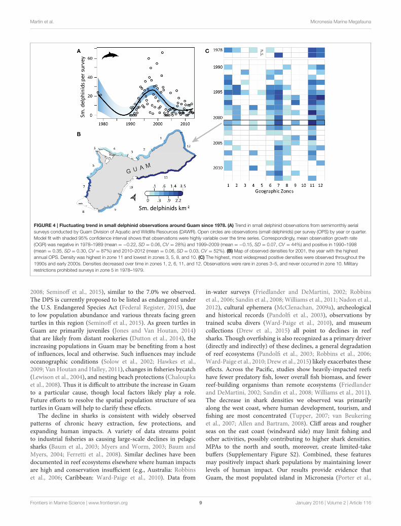
Small DelphinidsSmall delphinid observations fluctuated over time (Figure 4A)and space, with the highest densities and most consistentsightings along the southwest and northeast coasts, where reefsand sand dominated the benthic habitat and human densitieswere relatively low. OPS ranged from 0 to 38.2 across years(mean = 13.5, SD = 10.6, CV = 79%). OGR varied overtime; it was negative in 1978–1989 (mean = −0.22, SD =

0.06, CV = 28%; but note there are only 3 points in thisperiod, Figure 4A) and 1999–2009 (mean = −0.15, SD = 0.07,CV = 44%), and positive in 1990–1998 (mean = 0.35, SD =

0.30, CV = 87%) and 2010–2012 (mean = 0.06, SD = 0.03,CV = 52%). Due to these changes in the direction of OGR, itsvariability across all years was extremely high (mean = 0.05, SD= 0.30, CV = 611%). OPS was highest in 2001, when density

Frontiers in Marine Science | www.frontiersin.org 6 January 2016 | Volume 2 | Article 116

Martin et al. Micronesia Marine Megafauna

FIGURE 2 | Five-fold decline in reef shark observations around Guam in the last five decades. (A) Trend in shark observations from aerial surveys conducted

semimonthly by Guam Division of Aquatic and Wildlife Resources (DAWR). Observations (sharks) per survey (OPS) by year or quarter are indicated by open circles.

Smooth trend line and shaded 95% confidence interval are from a model fit. Since 1963, mean population growth rate (PGR) was −0.03 (SD = 0.04, CV = 138%). (B)

Map of observed densities for 1965, when annual OPS was highest; densities were particularly high for western zones 1–4, especially compared to densities there in

later years. (C) After 1976, west coast observations became sporadic and densities generally decreased. On the east coast (zones 9–11), densities were high through

the 1990s, then decreased slightly, but remained generally higher than west coast densities. No surveys occurred in zone 5 in 1975–1979 due to military restrictions.

reached 3.47 small delphinids km−2 along the northeast coast(zone 11) (Figure 4B). Intermediate densities (0.06–1.89 smalldelphinids km−2) occurred in most other areas in 2001, althoughno small delphinids were observed in zones 3 and 5 in thewest, 8 in the south, and 10 in the east (Figure 4B). Over time,historically high densities in the north (zone 12) and northeast(zone 11) decreased (Figure 4C). On the west coast, densitieswere consistently low in zones 3–5, while they were frequentlyintermediate in zones 1 and 7. Densities were high in many zonesduring the 1990s and early 2000s, after which they decreased andbecame more localized to fewer zones (7, 8, and 11). The highestmean densities for 2008–2012 occurred in zones 7 (0.57 smalldelphinids km−2; reef and sandy habitat; low human density), 11(0.18 small delphinids km−2; reef and sandy habitat; low/mediumhuman density; MPA along 23% of shoreline; military lands along24% of shoreline) and 4 (0.15 small delphinids km−2; reef habitat;low human density; MPA along 20% of shoreline; Table 1).

Large DelphinidsLarge delphinid observations were low, but increased slightlyover time (Figure 5A) and were most dense along the southwestand north coasts. OPS ranged from 0 to 1.43 across years (mean= 0.20, SD = 0.39, CV = 197%). OGR and its variability werehigh due to the low number of observations (mean = 0.16, SD= 0.83, CV = 508%); this OGR is particularly unreliable in a

population context, as it may reflect up to four species acrossonly six total encounters, and the survey area only captures asmall portion of the habitat range for those species. OPS washighest in 2010 (1.43 large delphinids per survey), when densitywas 0.55 large delphinids km−2 in the southwest (zone 7) and0 elsewhere (Figure 5B). Large delphinids were never observedin zones 1–5 on the west coast or zone 10 on the east coast(Figure 5C). Density was only positive in one zone per year, andonly in the south (zones 6–9) and northeast (zones 11–12). Since2007, observations have been slightly higher (mean density of0.014 vs. 0.001 prior to 2007) and more frequent (Figure 5C).Mean densities for 2008–2012 were highest in zones 7 (0.11 largedelphinids km−2; reef and sandy habitat; low human density),12 (0.07 large delphinids km−2; reef habitat; low/medium humandensity; MPA along 60% of shoreline; military lands along 65% ofshoreline), and 6 (0.02 large delphinids km−2; reef and seagrasshabitat; low/medium human density; military lands along 45% ofshoreline; Table 1).

DISCUSSION

Five decades of aerial surveys of Guam’s reefs provide importantinsights into changes in marine megafauna populations. Of thefive taxa we examined, turtles were the most widely distributedand consistently recorded, yet their dramatic increase was

Frontiers in Marine Science | www.frontiersin.org 7 January 2016 | Volume 2 | Article 116

Martin et al. Micronesia Marine Megafauna

FIGURE 3 | Infrequent, increasingly aggregated manta ray observations on Guam’s reefs since 1989. (A) Trend in manta ray observations from semimonthly

aerial surveys conducted by Guam Division of Aquatic and Wildlife Resources (DAWR). Observations (manta rays) per survey (OPS) by quarter are depicted with open

circles. Model fit with shaded 95% confidence interval suggests observations became slightly more common over time. Mean population growth rate (PGR) was 0.19

(SD = 0.61, CV = 321%), but should be viewed with caution due to the low number of observations. (B) Map of observed densities for 2010, the year with the highest

annual OPS; densities were high in the northwest (zones 1–2) and low elsewhere. (C) Since 2008, most observations were in the northwest, with a few sightings in the

southwest (zones 5, 6, and 8).

constrained to a single location. Shark numbers declined sharplyfrom early survey levels. Manta rays were infrequently seen,but observations increased slightly over time. Small delphinidnumbers fluctuated, with alternating regimes of decrease andincrease. Large delphinid observations were historically rare, butincreased slightly in the last decade. Each taxon had idiosyncraticspatial patterns, and was often clustered in specific zones of highdensities. For turtles, sharks, andmanta rays, the highest densities(2008–2012) were in zones that had coral reefs as dominanthabitat features and: (i) seagrass beds and sand flats as additionalhabitat features (turtles and sharks), (ii) low human densities(turtles and sharks), (iii) an MPA along >50% of the shoreline(turtles and manta rays), and (iv) an MPA along >50% of theadjacent zone’s shoreline (sharks and manta rays).

The observed increase in sea turtles in Guam is consistentwith the historical shift from extraction to conservationprotection. Previous studies have linked the low abundanceof sea turtle populations from 1950 to 1980 to historicalharvests (Groombridge et al., 1989; Van Houtan and Kittinger,2014) that occurred throughout the Pacific Islands. But seaturtle populations have been documented to rebound withconservation protections (e.g., Hawaii: Balazs and Chaloupka,2004); Costa Rica: Troëng and Rankin, 2005; and AscensionIsland: Broderick et al., 2006). The post-1999 increase weobserved occurred almost exclusively in zone 8, which contains

the Achang Reef Flat Preserve, a no-takeMPA established in 1997and fully enforced by 2001 (Tupper, 2007; Allen and Bartram,2008; Supplementary Figure S2). After 1999, observations werenearly 30 times higher in zone 8 but only 12% higher elsewhere(Supplementary Figure S3). Mangroves, seagrass beds, coralreefs, sand flats, and reef channels in this area provide qualityforaging and resting habitat for turtles (Tupper, 2007). Arecent global analysis showed satellite-tracked green turtlesdisproportionately aggregate in MPAs (Scott et al., 2012), whichis consistent with our results. However, our findings contrastwith those of Christianen et al. (2014), who found severelydegraded seagrass beds inside a 10-year old MPA where turtlesaggregated.

Our calculated rate of increase in Guam sea turtlescorroborates other regional time series, providing importantinformation for this data deficient region. Though thebiogeography and abundance of hawksbill populations ispoorly understood, the recent global green turtle status reviewplaced Guam within the Central West Pacific (CWP) distinctpopulation segment (DPS) (Seminoff et al., 2015). This DPSis spatially bounded by the Asian continent to the west andnorth, the Solomon Islands to the south, the Marshall Islands inthe east, and Palau in the west. The only long-term populationtime series from this DPS—from Chichijima in Ogasawara,Japan—had an annual growth rate of 6.8% (Chaloupka et al.,

Frontiers in Marine Science | www.frontiersin.org 8 January 2016 | Volume 2 | Article 116

Martin et al. Micronesia Marine Megafauna

FIGURE 4 | Fluctuating trend in small delphinid observations around Guam since 1978. (A) Trend in small delphinid observations from semimonthly aerial

surveys conducted by Guam Division of Aquatic and Wildlife Resources (DAWR). Open circles are observations (small delphinids) per survey (OPS) by year or quarter.

Model fit with shaded 95% confidence interval shows that observations were highly variable over the time series. Correspondingly, mean observation growth rate

(OGR) was negative in 1978–1989 (mean = −0.22, SD = 0.06, CV = 28%) and 1999–2009 (mean = −0.15, SD = 0.07, CV = 44%) and positive in 1990–1998

(mean = 0.35, SD = 0.30, CV = 87%) and 2010–2012 (mean = 0.06, SD = 0.03, CV = 52%). (B) Map of observed densities for 2001, the year with the highest

annual OPS. Density was highest in zone 11 and lowest in zones 3, 5, 8, and 10. (C) The highest, most widespread positive densities were observed throughout the

1990s and early 2000s. Densities decreased over time in zones 1, 2, 6, 11, and 12. Observations were rare in zones 3–5, and never occurred in zone 10. Military

restrictions prohibited surveys in zone 5 in 1978–1979.

2008; Seminoff et al., 2015), similar to the 7.0% we observed.The DPS is currently proposed to be listed as endangered underthe U.S. Endangered Species Act (Federal Register, 2015), dueto low population abundance and various threats facing greenturtles in this region (Seminoff et al., 2015). As green turtles inGuam are primarily juveniles (Jones and Van Houtan, 2014)that are likely from distant rookeries (Dutton et al., 2014), theincreasing populations in Guam may be benefiting from a hostof influences, local and otherwise. Such influences may includeoceanographic conditions (Solow et al., 2002; Hawkes et al.,2009; Van Houtan and Halley, 2011), changes in fisheries bycatch(Lewison et al., 2004), and nesting beach protections (Chaloupkaet al., 2008). Thus it is difficult to attribute the increase in Guamto a particular cause, though local factors likely play a role.Future efforts to resolve the spatial population structure of seaturtles in Guam will help to clarify these effects.

The decline in sharks is consistent with widely observedpatterns of chronic heavy extraction, few protections, andexpanding human impacts. A variety of data streams pointto industrial fisheries as causing large-scale declines in pelagicsharks (Baum et al., 2003; Myers and Worm, 2003; Baum andMyers, 2004; Ferretti et al., 2008). Similar declines have beendocumented in reef ecosystems elsewhere where human impactsare high and conservation insufficient (e.g., Australia: Robbinset al., 2006; Caribbean: Ward-Paige et al., 2010). Data from

in-water surveys (Friedlander and DeMartini, 2002; Robbinset al., 2006; Sandin et al., 2008; Williams et al., 2011; Nadon et al.,2012), cultural ephemera (McClenachan, 2009a), archeologicaland historical records (Pandolfi et al., 2003), observations bytrained scuba divers (Ward-Paige et al., 2010), and museumcollections (Drew et al., 2015) all point to declines in reefsharks. Though overfishing is also recognized as a primary driver(directly and indirectly) of these declines, a general degradationof reef ecosystems (Pandolfi et al., 2003; Robbins et al., 2006;Ward-Paige et al., 2010; Drew et al., 2015) likely exacerbates theseeffects. Across the Pacific, studies show heavily-impacted reefshave fewer predatory fish, lower overall fish biomass, and fewerreef-building organisms than remote ecosystems (Friedlanderand DeMartini, 2002; Sandin et al., 2008; Williams et al., 2011).The decrease in shark densities we observed was primarilyalong the west coast, where human development, tourism, andfishing are most concentrated (Tupper, 2007; van Beukeringet al., 2007; Allen and Bartram, 2008). Cliff areas and rougherseas on the east coast (windward side) may limit fishing andother activities, possibly contributing to higher shark densities.MPAs to the north and south, moreover, create limited-takebuffers (Supplementary Figure S2). Combined, these featuresmay positively impact shark populations by maintaining lowerlevels of human impact. Our results provide evidence thatGuam, the most populated island in Micronesia (Porter et al.,

Frontiers in Marine Science | www.frontiersin.org 9 January 2016 | Volume 2 | Article 116

Martin et al. Micronesia Marine Megafauna

FIGURE 5 | Rare, possibly increasing observations of large delphinids in coastal waters of Guam since 1989. (A) Trend in large delphinid observations from

aerial surveys conducted semimonthly by Guam Division of Aquatic and Wildlife Resources (DAWR). Open circles indicate quarterly observations (individuals) per

survey (OPS). Smoothed line and shading are from a model fit with 95% confidence interval. Observations were rare, with no large delphinids recorded in 75% of

survey years. (B) Map of observed densities for 2010, the year with the highest OPS. Density was positive in the southwest (zone 7), but zero elsewhere. (C) No large

delphinids were observed in zones 1–5 along the west coast or in zone 10 on the east coast. Large delphinids were recorded in a maximum of one zone per year

(zones 6–9 and 11–12). Sightings appear to be more frequent since 2007.

2005), follows the pattern of reef shark decline seen on otherreefs worldwide. Interestingly, the 84% decrease we observedfrom 1963 to 2012 (from our LOESS model) is not far fromthe 94% shark decline (from a pristine baseline) estimated forthe Mariana Islands from ecosystem models and towed-diversurvey data (Nadon et al., 2012). The aerial surveys began in1963, when conditions on Guam were already less than pristine,which may explain some of the difference in these estimates.Nonetheless, our results provide further support for the sharkdecline estimated by Nadon et al. (2012).

Trends for manta rays and cetaceans were less informative,but the spatial patterns provide insights into their distributionsaround Guam. The aggregation of manta rays in the northwestco-occurs with the Tumon Bay Marine Preserve (a limited-take MPA). At this site, manta rays were documented feedingon gamete clouds of spawning surgeonfish on the reef slope(Hartup et al., 2013). Unlike the other taxa, cetaceans do notdepend on the reefs to forage. The fluctuating temporal trendin small delphinid presence could be due to inter-annualvariability in the proximity of their prey to the coast. Andthough we believe most of the small delphinid sightings arespinner dolphins, observations of other species could obscurethe observed geographic or temporal signals. For both smalland large delphinids, the highest densities generally occur in thesouthwest and north/northeast, where reefs and sand flats aredominant habitat features and human density is relatively low;the Pati Point Preserve (a limited-take MPA adjacent to military

lands) is also located in the northeast (Supplementary Figure S2).This suggests that cetaceans may prefer areas with lower levelsof human activity. However, the mechanism driving theseobservations could be more related to oceanographic features,such as bathymetry and currents. These patterns deserve furtherattention.

Changes in survey techniques, detectability issues, and divingbehavior may affect our estimates of survey densities over thecourse of the study. We followed best practices recommendedfor addressing confounding factors when using historical ecologyapproaches (McClenachan et al., 2015), particularly in dealingwith species identification, variation in sampling effort, anddata gaps. For example, we aggregated species into broadtaxonomic groups, even though observers were fairly certainthey knew which species they observed. A disadvantage ofthis method is that trends for individual species are obscured.The shift from a helicopter in the 1960s to fixed-wing aircraftcould have influenced both observer visibility and airspeed,but these influences are uncertain. We assumed observersdetected all surface animals, but they may actually miss animals,biasing abundance estimates (Marsh and Sinclair, 1989; Seminoffet al., 2014; Fuentes et al., 2015). Bathymetric differences alsomay make detection easier in some geographic areas thanothers. Surface glare, cloud cover, and wave height may affectdetectability; we investigated the latter two and did not findrelationships with the number of animals observed. Further,observers may have become primed to expect animals in certain

Frontiers in Marine Science | www.frontiersin.org 10 January 2016 | Volume 2 | Article 116

Martin et al. Micronesia Marine Megafauna

areas and not others, based on previous experience or knowledgeof MPAs (Rocliffe et al., Unpublished data). They may missanimals when fishing activity is high, as monitoring fishing isthe primary objective. This risk may be minimized, however,through the use of highly experienced observers and voicerecorders. Our calculation of turtle abundances could be sensitiveto two conversion factors: (1) proportion of time spent at thesurface (availability), which may be impacted by the presence oftags (Jones et al., 2013), and (2) proportions of species in thepopulation.

Future studies could build on our analyses and strengthenour conclusions. First, digital video recorders or drones couldbe used to calibrate aerial observers and potentially conductsurveys. Calibration could provide useful data on observer-specific detection biases, and also validate the aerial surveysas effective means of collecting data on these taxa. Thesesurveys comprise a unique time series; confirming their use asa monitoring tool is important. Low-cost “conservation drones”have been successfully developed and used in tropical foreststo survey human activities and large animal species (Koh andWich, 2012) and could be an effective option for monitoring reefsystems. Second, standardized line-transect surveys (using aerialvehicles, manned or autonomous, or boats) could be conductedseparately for each taxon, with methods optimized for each. Suchsurveys would allow researchers to spend more time in each area.For cetaceans, the geographic scope could be expanded to includeareas beyond the reefs. For the reef-associated taxa (turtles,sharks, manta rays), studies could be designed at spatial scalesappropriate to compare densities inside and outside the MPAs;this would help determine whether they are having an impact.The 92-zone system could be used for spatial analyses. Third,future studies could examine protections, access (e.g., publicshoreline access locations), and extraction as potential driversof reef fauna densities in Guam by relating metrics of humanactivity (e.g., population, fishing, or land use) to those densities.Our study provided some context for this line of investigation,but did not attempt to identify cause-and-effect relationships.Finally, our continued efforts to capture and tag turtles willdecrease uncertainty in our abundance estimates by improvingdata on the two conversion factors. Efforts to tag reef sharks andmanta rays would provide information on the availability of thosetaxa at the surface, thus enabling estimates of abundance.

In this study, we analyzed five decades of aerial survey datafrom Guam to understand trends in abundance and distributionfor five marine megafauna, all of which are of conservationconcern and data deficient in this region. We showed that theobserved foraging population of turtles increased eight-fold,mostly in one geographic area with optimal habitat and MPA

status, while the observed reef shark population decreased 5-fold,mostly in areas proximate to human population centers. Trendsfor manta rays and cetaceans were less informative, but eachtaxon had geographic foci. Protections in the region may beworking to recover turtle populations, but failing (or have notyet had sufficient time) to recover overfished shark populations.Long-term analyses of vulnerable marine megafauna in this data-poor region are uncommon and should be used to guide morefocused studies. Furthermore, historical data and analyses suchas these should be considered in regional conservation andmanagement planning, as they provide important insights intopopulation and ecosystem changes, and baselines for calibratingrecovery goals (Van Houtan et al., 2012; Kittinger et al., 2013;McClenachan et al., 2015; Thurstan et al., 2015).

AUTHOR CONTRIBUTIONS

SM and KV designed the study. SW, JB, BT, JG, and CA collectedand maintained aerial data. TJ, SW, and JB collected turtle divedata. BT, KV, and SM digitized and quality-checked aerial data.TJ and KV quality-checked dive data. SM and KV analyzed data,prepared figures, and wrote the manuscript. All authors reviewedthe manuscript.

FUNDING

A portion of this research was funded by the Navy Commander,U.S. Pacific Fleet and the Naval Facilities Engineering Command(MIPR #N00070-13-MP-4C261).

ACKNOWLEDGMENTS

L. Mukai, C. Luecken, A. Soutar, and M. Suydam providedlogistical support to SM for the NRC RAP fellowship. J.Rivers, M. Kawai, S. Hakala, J. Whitaker, and E. Yago providedadministrative support for the Navy contract to KV. G. Balazs, E.Oleson, S. Kolinski, M. Hill, A. Bendlin, A. Bradford, R. Hensley,G. Davis, F. Parrish, and two reviewers provided constructivecomments on earlier versions of this manuscript. We thankall DAWR staff who contributed to the aerial surveys over theyears.

SUPPLEMENTARY MATERIAL

The Supplementary Material for this article can be foundonline at: http://journal.frontiersin.org/article/10.3389/fmars.2015.00116

REFERENCES

Allen, S., and Bartram, P. (2008). Guam as a Fishing Community. Administrative

Report H-08-01. Honolulu, HI: Pacific Islands Fisheries Science Center,National Marine Fisheries Service, NOAA.

Amesbury, J. R., and Hunter-Anderson, R. L. (2003). Review of Archaeological and

Historical Data Concerning Reef Fishing in the US Flag Islands of Micronesia:

Guam and the Northern Mariana Islands. Final Report. Honolulu, HI: WesternPacific Regional Fishery Management Council.

Balazs, G. H., and Chaloupka, M. (2004). Thirty-year recovery trend in the oncedepleted Hawaiian green sea turtle stock. Biol. Conserv. 117, 491–498. doi:10.1016/j.biocon.2003.08.008

Ban, N. C., Hansen, G. J. A., Jones, M., and Vincent, A. C. J. (2009).Systematic marine conservation planning in data-poor regions: Socioeconomic

Frontiers in Marine Science | www.frontiersin.org 11 January 2016 | Volume 2 | Article 116

Martin et al. Micronesia Marine Megafauna

data is essential. Marine Policy 33, 794–800. doi: 10.1016/j.marpol.2009.02.011

Baum, J. K., and Myers, R. A. (2004). Shifting baselines and the decline of pelagicsharks in the Gulf of Mexico. Ecol. Lett. 7, 135–145. doi: 10.1111/j.1461-0248.2003.00564.x

Baum, J. K., Myers, R. A., Kehler, D. G., Worm, B., Harley, S. J., andDoherty, P. A. (2003). Collapse and conservation of shark populationsin the Northwest Atlantic. Science 299, 389–392. doi: 10.1126/science.1079777

Broderick, A. C., Frauenstein, R., Glen, F., Hays, G. C., Jackson, A. L., Pelembe,T., et al. (2006). Are green turtles globally endangered? Glob. Ecol. Biogeogr. 15,21–26. doi: 10.1111/j.1466-822X.2006.00195.x

Brown, J. H., Whitham, T. G., Ernest, S. K., and Gehring, C. A. (2001).Complex species interactions and the dynamics of ecological systems:long-term experiments. Science 293, 643–650. doi: 10.1126/science.293.5530.643

Burdick, D. R. (2006). Guam Coastal Atlas Benthic Habitat Data (GIS

Layer). University of Guam Marine Laboratory & NOAA Pacific Islands

Fisheries Science Center. Available online at: http://www.guammarinelab.com/coastal.atlas/data/Guam_Coastal_Atlas_Benthic_Habitat_Data_Metadata.htm

Chaloupka, M., Bjorndal, K. A., Balazs, G. H., Bolten, A. B., Ehrhart, L. M.,Limpus, C. J., et al. (2008). Encouraging outlook for recovery of a onceseverely exploited marine megaherbivore. Glob. Ecol. Biogeogr. 17, 297–304.doi: 10.1111/j.1466-8238.2007.00367.x

Christianen, M. J., Herman, P. M., Bouma, T. J., Lamers, L. P., van Katwijk, M. M.,van der Heide, T., et al. (2014). Habitat collapse due to overgrazing threatensturtle conservation in marine protected areas. Proc. R. Soc. Lond. B Biol. Sci.

281:20132890. doi: 10.1098/rspb.2013.2890Cleveland,W. S., and Devlin, S. J. (1988). Locally weighted regression: an approach

to regression analysis by local fitting. J. Am. Statist. Assoc. 83, 596–610. doi:10.1080/01621459.1988.10478639

Drew, J. A., Amatangelo, K. L., andHufbauer, R. A. (2015). Quantifying theHumanImpacts on Papua New Guinea Reef Fish Communities across Space and Time.PLoS ONE 10:e0140682. doi: 10.1371/journal.pone.0140682

Dulvy, N. K., Baum, J. K., Clarke, S., Compagno, L. J. V., Cortés, E., Domingo,A., et al. (2008). You can swim but you can’t hide: the global status andconservation of oceanic pelagic sharks and rays. Aquat. Conserv. 18, 459–482.doi: 10.1002/aqc.975

Dutton, P. H., Jensen, M. P., Frutchey, K., Frey, A., LaCasella, E., Balazs, G.H., et al. (2014). Genetic stock structure of green turtle (Chelonia mydas)nesting populations across the Pacific islands. Pacific Sci. 68, 451–464. doi:10.2984/68.4.1

ESRI (2012). ArcMap 10.1 Desktop. Redlands, CA: Environmental SystemsResearch Institute Inc.

Federal Register (2015). Endangered and Threatened Species; Identification and

Proposed Listing of Eleven Distinct Population Segments of Green Sea Turtles

(Chelonia mydas) as Endangered or Threatened and Revision of Current Listings,

Vol. 80. Washington, DC: NOAA Fisheries and US Fish and Wildlife Service.Ferretti, F., Myers, R. A., Serena, F., and Lotze, H. K. (2008). Loss of large

predatory sharks from the Mediterranean Sea. Conserv. Biol. 22, 952–964. doi:10.1111/j.1523-1739.2008.00938.x

Forney, K. A., and Barlow, J. (1998). Seasonal patterns in the abundanceand distribution of California cetaceans, 1991–1992. Mar. Mammal Sci. 14,460–489. doi: 10.1111/j.1748-7692.1998.tb00737.x

Friedlander, A. M., and DeMartini, E. E. (2002). Contrasts in density, size, andbiomass of reef fishes between the northwestern and themainHawaiian islands:the effects of fishing down apex predators.Mar. Ecol. Progr. Ser. 230, e264. doi:10.3354/meps230253

Fuentes, M. M. P. B., Bell, I., Hagihara, R., Hamann, M., Hazel, J., Huth, A., et al.(2015). Improving in-water estimates of marine turtle abundance by adjustingaerial survey counts for perception and availability biases. J. Exp.Mar. Biol. Ecol.

471, 77–83. doi: 10.1016/j.jembe.2015.05.003Google (2013). Google Earth Pro 7.1.1.1580 (beta). Mountain View, CA: Google

Inc.Groombridge, B., and Luxmoore, R. A. (1989). The Green Turtle and Hawksbill

(Reptilia: Cheloniidae): World Status, Exploitation and Trade. Cambridge, UK:Secretariat of the Convention on International Trade in Engangererd Species ofWild Fauna and Flora.

Guidetti, P., and Micheli, F. (2011). Ancient art serving marine conservation.Front. Ecol. Environ. 9, 374–375. doi: 10.1890/11.WB.019

Hartup, J., Marshell, A., Stevens, G., Kottermair, M., and Carlson, P. (2013). Mantaalfredi target multispecies surgeonfish spawning aggregations. Coral Reefs 32,367–367. doi: 10.1007/s00338-013-1022-4

Hawkes, L. A., Broderick, A. C., Godfrey, M. H., and Godley, B. J. (2009).Climate change and marine turtles. Endang. Species Res. 7, 137–154. doi:10.3354/esr00198

Hensley, R. A., and Sherwood, T. S. (1993). An overview of Guam’s inshorefisheries.Mar. Fisher. Rev. 55, 129–138.

Hill, M. C., Ligon, A. D., Deakos, M. H., A. C. Ü., Milette-Winfree, A., Bendlin, A.R., and Oleson, E. M. (2014). Cetacean Surveys in the Waters of the Southern

Mariana Archipelago (February 2010 – April 2014). Prepared for the U.S.

Pacific Fleet Environmental Readiness Office.Honolulu, HI: PIFSC Data ReportDR-14-013, NOAA Fisheries.

IUCN (2015). The IUCN Red List of Threatened Species. Version 2015.2. Availableonline at: www.iucnredlist.org. Downloaded on 14 August 2015

Jones, T. T., and Van Houtan, K. S. (2014). Sea Turtle Tagging in the Mariana

Islands Range Complex (MIRC). Honolulu, HI: Annual Progress Report to theNavy, NOAA Fisheries.

Jones, T. T., Van Houtan, K. S., Bostrom, B. L., Ostafichuk, P., Mikkelsen, J.,Tezcan, E., et al. (2013). Calculating the ecological impacts of animal–borneinstruments on aquatic organisms. Methods Ecol. Evol. 4, 1178–1186. doi:10.1111/2041-210X.12109

Kessel, S., Gruber, S., Gledhill, K., Bond, M., and Perkins, R. (2013). Aerial surveyas a tool to estimate abundance and describe distribution of a carcharhinidspecies, the lemon shark, negaprion brevirostris. J. Mar. Biol. 2013:597383. doi:10.1155/2013/597383

Kittinger, J. N., Van Houtan, K. S., McClenachan, L. E., and Lawrence, A. L.(2013). Using historical data to assess the biogeography of population recovery.Ecography 36, 868–872. doi: 10.1111/j.1600-0587.2013.00245.x

Koh, L. P., and Wich, S. A. (2012). Dawn of drone ecology: low-cost autonomousaerial vehicles for conservation. Trop. Conserv. Sci. 5, 121–132. Available onlineat: http://tropicalconservationscience.mongabay.com/content/v5/index-jun-12.html

Lewison, R. L., Crowder, L. B., Read, A. J., and Freeman, S. A. (2004).Understanding impacts of fisheries bycatch on marine megafauna. Trends Ecol.Evol. 19, 598–604. doi: 10.1016/j.tree.2004.09.004

Lotze, H. K., Coll, M., Magera, A. M., Ward-Paige, C., and Airoldi, L. (2011).Recovery of marine animal populations and ecosystems. Trends Ecol. Evol. 26,595–605. doi: 10.1016/j.tree.2011.07.008

Magurran, A. E., Baillie, S. R., Buckland, S. T., Dick, J. M., Elston, D. A., Scott, E.M., et al. (2010). Long-term datasets in biodiversity research and monitoring:assessing change in ecological communities through time. Trends Ecol. Evol. 25,574–582. doi: 10.1016/j.tree.2010.06.016

Marsh, H., and Sinclair, D. F. (1989). Correcting for visibility bias in striptransect aerial surveys of aquatic fauna. J. Wildl. Manag. 53, 1017–1024. doi:10.2307/3809604

McClenachan, L., (2009a). Documenting loss of large trophy fish from theFlorida Keys with historical photographs. Conserv, Biol. 23, 636–643. doi:10.1111/j.1523-1739.2008.01152.x

McClenachan, L., (2009b). Historical declines of goliath grouper populations inSouth Florida, USA. Endang. Spec. Res. 7, 175–181. doi: 10.3354/esr00167

McClenachan, L., Cooper, A. B., McKenzie, M. G., and Drew, J. A. (2015).The importance of surprising results and best practices in historical ecology.BioScience 65, 932–939. doi: 10.1093/biosci/biv100

Myers, R. A., and Worm, B. (2003). Rapid worldwide depletion of predatory fishcommunities. Nature 423, 280–283. doi: 10.1038/nature01610

Nadon, M. O., Baum, J. K., Williams, I. D., McPherson, J. M.,Zgliczynski, B. J., Richards, B. L., et al. (2012). Re-Creating MissingPopulation Baselines for Pacific Reef Sharks Recreación de las Líneasde Base Poblacionales Faltantes para Tiburones de Arrecife en elPacífico. Conserv. Biol. 26, 493–503. doi: 10.1111/j.1523-1739.2012.01835.x

Nurse, L., McLean, R., Agard, J., Briguglio, L., Duvat-Magnan, V., Pelesikoti, N.,et al. (2014). “Small Islands,” in Climate Change 2014: Impacts, Adaptation, and

Vulnerability. Part B: Regional Aspects. Contribution of Working Group II to

the Fifth Assessment Report of the Intergovernmental Panel on Climate Change,

Frontiers in Marine Science | www.frontiersin.org 12 January 2016 | Volume 2 | Article 116

Martin et al. Micronesia Marine Megafauna

eds V. R. Barros, C. B. Field, D. J. Dokken, M. D. Mastrandrea, K. J. Mach,T. E. Bilir, et al. (Cambridge; New York, NY: Cambridge University Press),1613–1654.

Pandolfi, J. M., Bradbury, R. H., Sala, E., Hughes, T. P., Bjorndal, K. A., Cooke,R. G., et al. (2003). Global trajectories of the long-term decline of coral reefecosystems. Science 301, 955–958. doi: 10.1126/science.1085706

Pimm, S. L. (1991). The Balance of Nature?: Ecological Issues in the

Conservation of Species and Communities. Chicago, IL: University of ChicagoPress.

Porter, V., Leberer, T., Gawel, M., Gutierrez, J., Burdick, D., Torres, V., et al.(2005). “The state of the coral reef ecosystems of Guam,” in The State of

the Coral Reef Ecosystems of the United States and Pacific Freely Associated

States, ed J. Waddell (Silver Spring, MD: NOAA/NCCOS Center for CoastalMonitoring and Assessment’s Biogeography Team), 442–487. NOAATechnicalMemorandum NOS NCCOS 11.

Pritchard, P. C. H. (1995). “Marine turtles of micronesia,” in Biology and

Conservation of Sea Turtles, ed K. A. Bjorndal (Washington, DC: SmithsonianInstitution Press), 263–274.

R Core Team. (2014). R: A Language and Environment for Statistical Computing.Vienna: R Foundation for Statistical Computing.

Robbins, W. D., Hisano, M., Connolly, S. R., and Choat, J. H. (2006). Ongoingcollapse of coral-reef shark populations. Curr. Biol. 16, 2314–2319. doi:10.1016/j.cub.2006.09.044

Sáenz-Arroyo, A., Roberts, C. M., Torre, J., Cariño-Olvera, M., and Enríquez-Andrade, R. (2005). Rapidly shifting environmental baselines among fishersof the Gulf of California. Proc. R. Soc. Lond. B Biol. Sci. 272, 1957–1962. doi:10.1098/rspb.2005.3175

Sandin, S. A., Smith, J. E., Demartini, E. E., Dinsdale, E. A., Donner, S. D.,Friedlander, A. M., et al. (2008). Baselines and degradation of coral reefs in theNorthern Line Islands. PLoS ONE 3:e1548. doi: 10.1371/journal.pone.0001548

Scott, R., Hodgson, D. J., Witt, M. J., Coyne, M. S., Adnyana, W., Blumenthal,J. M., et al. (2012). Global analysis of satellite tracking data shows that adultgreen turtles are significantly aggregated in Marine Protected Areas. Glob. Ecol.Biogeogr. 21, 1053–1061. doi: 10.1111/j.1466-8238.2011.00757.x

Seminoff, J. A., Allen, C. D., Balazs, G. H., Dutton, P. H., Eguchi, T., Haas, H. L.,et al. (2015). Status Review of the Green Turtle (Chelonia mydas) Under the

U.S. Endangered Species Act. La Jolla, CA: NOAA Technical Memorandum,NOAA-NMFS-SWFSC-539.

Seminoff, J. A., Eguchi, T., Carretta, J., Allen, C. D., Prosperi, D., Rangel, R.,et al. (2014). Loggerhead sea turtle abundance at a foraging hotspot in theeastern Pacific Ocean: implications for at-sea conservation. Endang. Spec. Res.24, 207–220. doi: 10.3354/esr00601

Solow, A. R., Bjorndal, K. A., and Bolten, A. B. (2002). Annual variation innesting numbers of marine turtles: the effect of sea surface temperatureon re−migration intervals. Ecol. Lett. 5, 742–746. doi: 10.1046/j.1461-0248.2002.00374.x

Thurstan, R. H., McClenachan, L., Crowder, L. B., Drew, J. A., Kittinger,J. N., Levin, P. S., et al. (2015). Filling historical data gaps to fostersolutions in marine conservation. Ocean Coast. Manag. 115, 31–40. doi:10.1016/j.ocecoaman.2015.04.019

Troëng, S., and Rankin, E. (2005). Long-term conservation efforts contribute topositive green turtle Chelonia mydas nesting trend at Tortuguero, Costa Rica.Biol. Conserv. 121, 111–116. doi: 10.1016/j.biocon.2004.04.014

Tupper, M. H. (2007). Spillover of commercially valuable reef fishes from marineprotected areas in Guam, Micronesia. Fish. Bull. 105, 527–537. Available onlineat: http://fishbull.noaa.gov/1054/tupper.pdf

U.S. Census Bureau (2010). 2010 Census Island Areas: Guam. Availableonline at: https://www.census.gov/2010census/news/press-kits/island-areas/island-areas.html

van Beukering, P., Haider, W., Longland, M., Cesar, H., Sablan, J., Shjegstad, S.,et al. (2007). The Economic Value of Guam’s Coral Reefs. Mangilao: Universityof GuamMarine Laboratory.

Van Houtan, K. S., and Halley, J. M. (2011). Long-term climateforcing in loggerhead sea turtle nesting. PLoS ONE 6:e19043. doi:10.1371/journal.pone.0019043

Van Houtan, K. S., and Kittinger, J. N. (2014). Historical commercial exploitationand the current status of Hawaiian green turtles. Biol. Conserv. 170, 20–27. doi:10.1016/j.biocon.2013.11.011

Van Houtan, K. S., Kittinger, J. N., Lawrence, A. L., Yoshinaga, C., Born, V. R.,and Fox, A. (2012). Hawksbill sea turtles in the northwestern Hawaiian Islands.Chelonian Conserv. Biol. 11, 117–121. doi: 10.2744/CCB-0984.1

Van Houtan, K. S., McClenachan, L., and Kittinger, J. N. (2013). Seafood menusreflect long-term ocean changes. Front. Ecol. Environ. 11, 289–290. doi:10.1890/13.WB.015

Ward-Paige, C. A., Mora, C., Lotze, H. K., Pattengill-Semmens, C., McClenachan,L., Arias-Castro, E., et al. (2010). Large-scale absence of sharks on reefs in theGreater-Caribbean: a footprint of human pressures. PLoS ONE 5:e11968. doi:10.1371/journal.pone.0011968

Wiles, G. J., Aguon, C. F., Davis, G., and Grout, D. (1995). The status anddistribution of endangered animals and plants in northern Guam.Micronesica

28, 31–49.Williams, I. D., Richards, B. L., Sandin, S. A., Baum, J. K., Schroeder, R. E., Nadon,

M. O., et al. (2011). Differences in reef fish assemblages between populatedand remote reefs spanning multiple archipelagos across the central and westernPacific. J. Mar. Biol. 2011:826234. doi: 10.1155/2011/826234

Willis, K. J., and Birks, H. J. B. (2006). What is natural? The need for a long-term perspective in biodiversity conservation. Science 314, 1261–1265. doi:10.1126/science.1122667

Conflict of Interest Statement: The authors declare that the research wasconducted in the absence of any commercial or financial relationships that couldbe construed as a potential conflict of interest.

Copyright © 2016 Martin, Van Houtan, Jones, Aguon, Gutierrez, Tibbatts, Wusstig

and Bass. This is an open-access article distributed under the terms of the Creative

Commons Attribution License (CC BY). The use, distribution or reproduction in

other forums is permitted, provided the original author(s) or licensor are credited

and that the original publication in this journal is cited, in accordance with accepted

academic practice. No use, distribution or reproduction is permitted which does not

comply with these terms.

Frontiers in Marine Science | www.frontiersin.org 13 January 2016 | Volume 2 | Article 116