fitting and simulation of models for telecommunication ... · fitting and simulation of models for...

Fitting and Simulation of Models forTelecommunication Access Networks

Frank FleischerJoint work with C. Gloaguen, H. Schmidt, V. Schmidt

University of Ulm

Department of Applied Information Processing

Department of Stochastics

France Telecom R & D, Paris

Workshop Freudenstadt 2005, Frank Fleischer 1

Outline

Stochastic–geometric network modellingAims

The Stochastic Subscriber Line Model

Models for the road systemRandom tessellations

Nestings of tessellations

Model choice procedureModel choice based on distance measures

Results for real input data

Typical Cox-Voronoi cellsSimulation algorithm

Results


Stochastic–geometric network modellingAims

Aims of modellingCost analysis and risk evaluationAnalysis of performance indicatorsSimulation of present and future network designscenariosDescription of the network by a minimum number ofstructural parameters

Models are necessary both for the road system and forthe telecommunication equipment

The model choice has to be based on the statisticalanalysis of real network data as well as of simulatednetwork data


Stochastic–geometric network modellingInfrastructure system of Paris


Stochastic–geometric network modellingStochastic Subscriber Line Model (SSLM)

System of main roads



System of main roads and side streets



Placement of network nodes and their serving zones


Models for the road systemRandom tessellations

A sequence {Pn}n≥1 of convex polytopes Pn ∈ IR2 iscalled (deterministic) tessellation of IR2 if

int Pn 6= ∅ for all n ≥ 1

int Pn ∩ int Pm = ∅ for all n 6= m

S∞n=1

Pn = IR2

P

n≥1

1{Pn∩K 6=∅} < ∞ for all compact sets K ∈ IR2

The Pn’s are called cells of the tessellation

A sequence X0 = {Ξn}n≥1 of random convex polytopesis called random tessellation of IR2 if

IP(X0 ∈ T ) = 1 ,

where T denotes the family of all tessellations in IR2


Models for the road systemPoisson line tessellation (PLT)

Realization of PLT

Induced by Poissonline process

The intensity γPLT isthe mean total length oflines per unit area

Notice: 2γPLT is themean number of linesintersecting the unit ball


Models for the road systemPoisson–Voronoi tessellation (PVT)

Realization of PVT

Cells are formed withrespect to a set ofnuclei

The intensity γPV T isthe mean number of nu-clei per unit area


Models for the road systemPoisson–Delaunay tessellation (PDT)

Realization of PDT

Cells are triangles

Vertices are nuclei of aPVT

The intensity γPDT isthe mean number ofvertices per unit area


Models for the road systemSome characteristics of random tessellations

Realization of PLT

Global characteristicsλ1 mean number of vertices

λ2 mean number of edges

λ3 mean number of cells

λ4 mean total length of

edges

Local characteristicsmean perimeter

mean area


Models for the road systemSome characteristics of random tessellations

Tessellation λ1 λ2 λ3 λ4

PLT 1πγ2 2

πγ2 1

πγ2 γ

PVT 2γ 3γ γ 2√

γ

PDT γ 3γ 2γ 323π

√γ

Values of λ1, . . . , λ4 for a tessellation with intensity γ


Models for the road systemRandom nestings of tessellations

A (deterministic) iterated tessellations of IR2 is given by

{Pn ∩ Pnν : int Pn ∩ int Pnν 6= ∅ ; n, ν ∈ N}an initial tessellation {Pn}n≥1

a sequence ({Pnν}ν≥1)n≥1 of component tessellations

A (random) nesting of tessellations in IR2 is given by

{Ξn ∩ Ξnν : int Ξn ∩ int Ξnν 6= ∅ ; n, ν ∈ N}X0 = {Ξn}n≥1 is an arbitrary random tessellation in IR2

{Xn}n≥1 = ({Ξnν}ν≥1)n≥1 is an independent sequence of independent

and identically distributed random tessellations in IR2

Notation: X0/X1–nesting



PLT/PVT–nesting PDT/PLT–nesting



PVT/PVT–nesting PLT/PVT-nesting

Nestings with Bernoulli thinning (p = 0.75)


Models for the road systemSome characteristics of random nestings

PVT/PVT-nesting

Characteristics of X0

(λ(0)1 , λ

(0)2 , λ

(0)3 , λ

(0)4 )

Characteristics of X1

(λ(1)1 , λ

(1)2 , λ

(1)3 , λ

(1)4 )

Measured per unit area


Models for the road systemSome characteristics of random nestings

Joint characteristics of X0/pX1–nesting

λ1 = λ(0)1 + pλ

(1)1 +

4p

πλ

(0)4 λ

(1)4

λ2 = λ(0)2 + pλ

(1)2 +

6p

πλ

(0)4 λ

(1)4

λ3 = λ(0)3 + pλ

(1)3 +

2p

πλ

(0)4 λ

(1)4

λ4 = λ(0)4 + pλ

(1)4

⇒ Formulae for nestings involving PLT, PDT and PVT


Idea of the model choiceReal network data


Idea of the model choiceReal network data

Data possess certainhierarchical structure

Examples of datacharacteristics

Number of road intersections

(λ1)

Number of edges (λ2)

Number of cells (λ3)

Total length of roads (λ4)

Real network data and their characteristics


Idea of the model choiceSummary

Observe input data in sampling window W

Get vector of estimates

λinp = (λinp

1 , λinp2 , λinp

3 , λinp4 )

from input data by using unbiased estimators

For certain values of γ (or γ0 and γ1) compute theentries λ1, λ2, λ3, and λ4 of λ

Minimize distance d(λinp,λ) ⇒ dmin(λinp,λ)

Repeat for all competing models: λopt and γopt

Validation by Monte-Carlo tests


Model choice procedureRelative distance measures

Let x = (x1, . . . , xn) and y = (y1, . . . , yn) denote twovectors

Euclidean distance

de(x,y) =

√

√

√

√

n∑

i=1

(

xi − yi

xi

)2

Absolute value distance

da(x,y) =n

∑

i=1

∣

∣

∣

∣

xi − yi

xi

∣

∣

∣

∣

Maximum norm distance

dm(x,y) = maxi=1,...,n

∣

∣

∣

∣

xi − yi

xi

∣

∣

∣

∣


Model choice procedureOptimization of distances

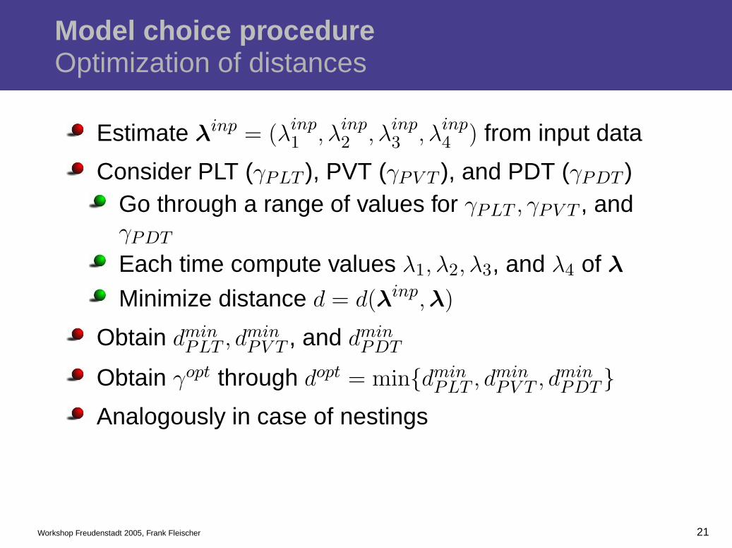
Estimate λinp = (λinp

1 , λinp2 , λinp

3 , λinp4 ) from input data

Consider PLT (γPLT ), PVT (γPV T ), and PDT (γPDT )Go through a range of values for γPLT , γPV T , andγPDT

Each time compute values λ1, λ2, λ3, and λ4 of λ

Minimize distance d = d(λinp,λ)

Obtain dminPLT , dmin

PV T , and dminPDT

Obtain γopt through dopt = min{dminPLT , dmin

PV T , dminPDT }

Analogously in case of nestings


Numerical examplesSimulated input data

Consider PLT with γ = 0.1

Quadratic sampling window (side length 10000)

Estimated Theoretical

λ1 0.00318 0.00318

λ2 0.00630 0.00637

λ3 0.00318 0.00318

λ4 0.09995 0.10000

Estimated and theoretical characteristics of the PLT



Let γ ∈ [0.0001, 0.5], step width 10−5

de,min γ da,min γ dm,min γ

PLT 0.0075 0.0998 0.0102 0.0999 0.0049 0.0997

PVT 0.4672 0.0020 0.7450 0.0021 0.3349 0.0021

PDT 0.6455 0.0017 1.0968 0.0016 0.4372 0.0018

Estimated and theoretical characteristics of the PLT



X0 = PLT (γ0 = 0.08), X1 = PDT (γ1 = 0.0008)

Quadratic sampling window (side length 10000)

Estimated Theoretical

λ1 0.01231 0.012619

λ2 0.02165 0.021147

λ3 0.00829 0.008528

λ4 0.17433 0.176034

Estimated and theoretical characteristics of thePLT/PDT–nesting



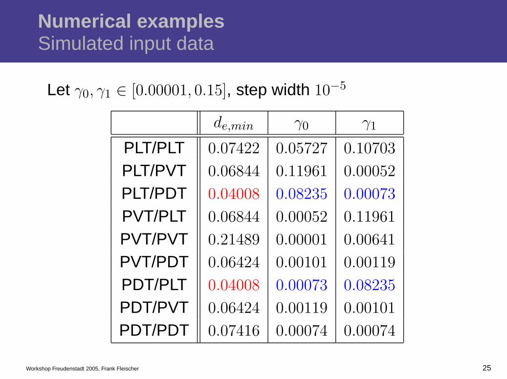
Let γ0, γ1 ∈ [0.00001, 0.15], step width 10−5

de,min γ0 γ1

PLT/PLT 0.07422 0.05727 0.10703

PLT/PVT 0.06844 0.11961 0.00052

PLT/PDT 0.04008 0.08235 0.00073

PVT/PLT 0.06844 0.00052 0.11961

PVT/PVT 0.21489 0.00001 0.00641

PVT/PDT 0.06424 0.00101 0.00119

PDT/PLT 0.04008 0.00073 0.08235

PDT/PVT 0.06424 0.00119 0.00101

PDT/PDT 0.07416 0.00074 0.00074



Solutions for problem of ambiguous decisions

If thinning factor p < 1 decisions uniqueIntroduce p as additional optimization parameterIncreases runtimeSometimes p known

Iterative fitting procedureFitting procedure for X0

Fitting of nesting with X0 givenHierarchical data structure needed


Numerical examplesReal input data

(a) Raw data (b) Preprocessed data

Data of a local region within Paris



Decide between PLT, PVT, and PDT

Let γ ∈ [10−6, 0.03], step width 10−8

Tessellation de,min γ

PLT 0.29555 0.016922

PVT 0.20147 0.000065

PDT 0.77293 0.000046

Decision in favor of PVT with γ = 0.000065



Decision for a PVT is obvious?

Idea: Consider main roads first

Tessellation de,min γ

PLT 0.21101 0.002384

PVT 0.29749 0.000001

PDT 0.73378 0.000001

Main roads would be modeled by PLT with γ = 0.002384



Decide between PLT/PLT, PLT/PVT, and PLT/PDT

X de,min γ0 γ1

PLT/PLT 0.15224 0.002384 0.013906

PLT/PVT 0.20455 0.002384 0.000044

PLT/PDT 0.36649 0.002384 0.000028

Road system would be modeled by PLT/PLT–nesting withγ0 = 0.002384 and γ1 = 0.013906


Typical Cox-Voronoi cells

For main roads decision mostly in favor of PLT

Higher-level telecommuncation equipment placed onmain roads only

Placement modeled by linear Poisson processesCox processes induced by Poisson line processesTypical serving zones of interestTypical cells of Cox-Voronoi tessellation (CVT)’Typical’ means drawing uniformly from all cells

Simulation algorithm based on Slyvniak’s theorem

Usage of properties of Poisson point processes andPoisson line processes



Realization of a PLTWorkshop Freudenstadt 2005, Frank Fleischer 32


Random placement of points on PLTWorkshop Freudenstadt 2005, Frank Fleischer 32


Cox-Voronoi cellsWorkshop Freudenstadt 2005, Frank Fleischer 32


Starting line with initial nucleusWorkshop Freudenstadt 2005, Frank Fleischer 33


Placement of neighboring nucleiWorkshop Freudenstadt 2005, Frank Fleischer 33


Second line with points on itWorkshop Freudenstadt 2005, Frank Fleischer 33


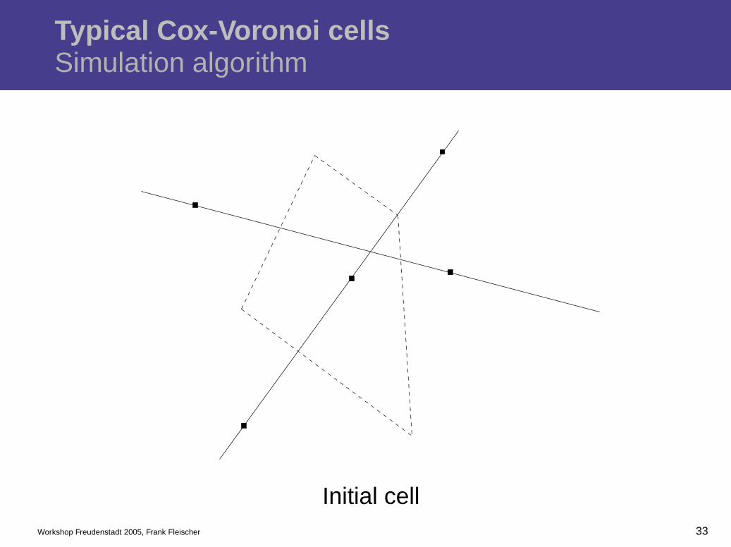
Initial cellWorkshop Freudenstadt 2005, Frank Fleischer 33


Stopping criterionWorkshop Freudenstadt 2005, Frank Fleischer 33


Cutting the initial cellWorkshop Freudenstadt 2005, Frank Fleischer 33


Typical Cox-Voronoi cellWorkshop Freudenstadt 2005, Frank Fleischer 33

Typical Cox-Voronoi cellsScaling property

Typical cell can be analyzed regarding geometriccharacteristics (e.g. area, perimeter, number ofvertices, shape,..)

Model parametersγ (intensity of line tessellation)λC (intensity of components on the lines)λ = γλC (intensity of the point process with respectto unit area)

Scaling propertySame structure but on a different scaleκ = γ/λC important parameter1/γ good measure for scale


Typical Cox-Voronoi cellsScaling property

Scaling property, different intensities but same κ


Typical Cox-Voronoi cellsResults

Estimations for first order and second order momentsof geometric characteristics for any given pair (γ∗, λ∗

C)

Information about distribution of geometriccharacteristics (=> risk analysis)

Similarities to typical cell of Poisson-Voronoitessellation, especially for large κ

Useful for simulation of network characteristicsMean shortest path lengthsMean subscriber line lengths


References

C. Gloaguen, F. Fleischer, H. Schmidt and V. SchmidtFitting of stochastic telecommunication network models viadistance measures and Monte-Carlo tests.Preprint (submitted to Telecommunication Systems),2004.

C. Gloaguen, F. Fleischer, H. Schmidt and V. SchmidtSimulation of typical Cox-Voronoi cells, with a special regard toimplementation tests.Preprint (submitted to Mathematical Methods ofOperations Research), 2005.

See also www.geostoch.de.


fitting and simulation of models for telecommunication ... · fitting and simulation of models for...

Documents