simulation, fitting, statistics and plotting. reference...
TRANSCRIPT

SIMFITSIMFITSIMFITSIMFITSIMFITSIMFITSIMFITSIMFITSIMFITSIMFITSIMFITSIMFITSIMFITSIMFITSIMFITSIMFITSIMFITSIMFITSIMFITSIMFITSIMFITSIMFITSIMFITSIMFITSIMFITSIMFITSIMFITSIMFITSIMFITSIMFITSIMFITSIMFITSIMFITSIMFITSIMFITSIMFITSIMFITSIMFITSIMFITSimulation, fitting, statistics and plotting.
REFERENCE MANUALhttp://www.simfit.man.ac.uk
-1
1
-1 1
Rhodoneae of Abbe Grandi, r = sin(4 )
x
y
100%
80%
60%
40%
20%
0%
PC1PC2
PC5PC8
PC6HC8
PC3PC4
PC7HC7
HC424A
33B76B
30B100A
34
53A
76
30A
61B60A
27A27B
52
37B
68
28A
97A26A
60B29
36A36B
31B31A
35B32A
32B35A
72A72B
99A99B
37A47
100B33A
53B73
24B26B
28B97B
91A91B
25A25B
61AHC5
HC6
Per
cent
age
Sim
ilarit
y
Bray-Curtis Similarity Dendrogram
0.00
0.25
0.50
0.75
1.00
0.00 0.50 1.00 1.50 2.00
Scatchard Plot for the 2 2 isoform
y
y/x
(µM
-1)
1 Site Model
2 Site Model
T = 21°C[Ca++] = 1.3×10⁻⁷M
0.000
0.100
0.200
0.300
0.400
0.500
-3.0 1.5 6.0 10.5 15.0
Deconvolution of 3 Gaussians
x
y
Values
Month 7Month 6
Month 5Month 4
Month 3Month 2
Month 1
Case 1Case 2
Case 3Case 4
Case 5
0
11
Simfit Cylinder Plot with Error Bars
0
20
40
60
80
100
0 20 40 60 80
ANOVA (k = no. groups, n = no. per group)
Sample Size (n)
Pow
er (
%)
k =
2k
= 4
k =
8k
= 16
k =
32
2 = 1 (variance) = 1 (difference)
Version 5.6.25


Contents
1 Overview 11.1 Installation . . . . . . . . . . . . . . . . . . . . . . . . . . . . . . . . . . . . . . . . . . . 21.2 Documentation. . . . . . . . . . . . . . . . . . . . . . . . . . . . . . . . . . . . . . . . . 21.3 Plotting . . . . . . . . . . . . . . . . . . . . . . . . . . . . . . . . . . . . . . . . . . . . . 3
2 First time user’s guide 72.1 The main menu. . . . . . . . . . . . . . . . . . . . . . . . . . . . . . . . . . . . . . . . . 72.2 The task bar. . . . . . . . . . . . . . . . . . . . . . . . . . . . . . . . . . . . . . . . . . . 92.3 The file selection control. . . . . . . . . . . . . . . . . . . . . . . . . . . . . . . . . . . . 10
2.3.1 Multiple file selection . . . . . . . . . . . . . . . . . . . . . . . . . . . . . . . . . 112.3.1.1 The project technique. . . . . . . . . . . . . . . . . . . . . . . . . . . . 122.3.1.2 Checking and archiving project files. . . . . . . . . . . . . . . . . . . . 12
2.4 First time user’s guide to data handling. . . . . . . . . . . . . . . . . . . . . . . . . . . . . 132.4.1 The format for input data files. . . . . . . . . . . . . . . . . . . . . . . . . . . . . 132.4.2 File extensions and folders. . . . . . . . . . . . . . . . . . . . . . . . . . . . . . . 132.4.3 Advice concerning data files. . . . . . . . . . . . . . . . . . . . . . . . . . . . . . 132.4.4 Advice concerning curve fitting files. . . . . . . . . . . . . . . . . . . . . . . . . . 132.4.5 Example 1: Making a curve fitting file. . . . . . . . . . . . . . . . . . . . . . . . . 142.4.6 Example 2: Editing a curve fitting file. . . . . . . . . . . . . . . . . . . . . . . . . 142.4.7 Example 3: Making a library file. . . . . . . . . . . . . . . . . . . . . . . . . . . . 142.4.8 Example 4: Making a vector/matrix file. . . . . . . . . . . . . . . . . . . . . . . . 152.4.9 Example 5: Editing a vector/matrix file. . . . . . . . . . . . . . . . . . . . . . . . 152.4.10 Example 6: Saving data-base/spread-sheet tables tofiles . . . . . . . . . . . . . . . 15
2.5 First time user’s guide to graph plotting. . . . . . . . . . . . . . . . . . . . . . . . . . . . 162.5.1 The SIMFIT simple graphical interface. . . . . . . . . . . . . . . . . . . . . . . . 162.5.2 The SIMFIT advanced graphical interface. . . . . . . . . . . . . . . . . . . . . . . 172.5.3 PostScript,GSview/Ghostscript and SIMFIT . . . . . . . . . . . . . . . . . . . . . 192.5.4 Example 1: Creating a simple graph. . . . . . . . . . . . . . . . . . . . . . . . . . 212.5.5 Example 2: Error bars. . . . . . . . . . . . . . . . . . . . . . . . . . . . . . . . . 212.5.6 Example 3: Histograms and cumulative distributions. . . . . . . . . . . . . . . . . 222.5.7 Example 4: Double graphs with two scales. . . . . . . . . . . . . . . . . . . . . . 222.5.8 Example 5: Bar charts. . . . . . . . . . . . . . . . . . . . . . . . . . . . . . . . . 232.5.9 Example 6: Pie charts. . . . . . . . . . . . . . . . . . . . . . . . . . . . . . . . . 242.5.10 Example 7: Surfaces, contours and 3D bar charts. . . . . . . . . . . . . . . . . . . 24
2.6 First time user’s guide to curve fitting. . . . . . . . . . . . . . . . . . . . . . . . . . . . . 252.6.1 User friendly curve fitting programs. . . . . . . . . . . . . . . . . . . . . . . . . . 262.6.2 IFAIL and IOSTAT error messages. . . . . . . . . . . . . . . . . . . . . . . . . . . 262.6.3 Example 1: Exponential functions. . . . . . . . . . . . . . . . . . . . . . . . . . . 272.6.4 Example 2: Nonlinear growth and survival curves. . . . . . . . . . . . . . . . . . . 282.6.5 Example 3: Enzyme kinetic and ligand binding data. . . . . . . . . . . . . . . . . 29
2.7 First time user’s guide to simulation. . . . . . . . . . . . . . . . . . . . . . . . . . . . . . 312.7.1 Why fit simulated data ?. . . . . . . . . . . . . . . . . . . . . . . . . . . . . . . . 31
i

ii Contents
2.7.2 Programsmakdat andadderr . . . . . . . . . . . . . . . . . . . . . . . . . . . . . 312.7.3 Example 1: Simulatingy = f (x) . . . . . . . . . . . . . . . . . . . . . . . . . . . . 312.7.4 Example 2: Simulatingz= f (x,y) . . . . . . . . . . . . . . . . . . . . . . . . . . . 322.7.5 Example 3: Simulating experimental error. . . . . . . . . . . . . . . . . . . . . . . 322.7.6 Example 4: Simulating differential equations. . . . . . . . . . . . . . . . . . . . . 332.7.7 Example 5: Simulating user-defined equations. . . . . . . . . . . . . . . . . . . . 34
3 Data analysis techniques 353.1 Types of data and measurement scales. . . . . . . . . . . . . . . . . . . . . . . . . . . . . 353.2 Principles involved when fitting models to data. . . . . . . . . . . . . . . . . . . . . . . . 35
3.2.1 Limitations when fitting models. . . . . . . . . . . . . . . . . . . . . . . . . . . . 363.2.2 Fitting linear models. . . . . . . . . . . . . . . . . . . . . . . . . . . . . . . . . . 373.2.3 Fitting generalized linear models. . . . . . . . . . . . . . . . . . . . . . . . . . . . 373.2.4 Fitting nonlinear models. . . . . . . . . . . . . . . . . . . . . . . . . . . . . . . . 383.2.5 Fitting survival models. . . . . . . . . . . . . . . . . . . . . . . . . . . . . . . . . 383.2.6 Distribution of statistics from regression. . . . . . . . . . . . . . . . . . . . . . . . 38
3.2.6.1 The chi-square test for goodness of fit. . . . . . . . . . . . . . . . . . . 393.2.6.2 Thet test for parameter redundancy. . . . . . . . . . . . . . . . . . . . . 393.2.6.3 TheF test for model discrimination. . . . . . . . . . . . . . . . . . . . . 393.2.6.4 Analysis of residuals. . . . . . . . . . . . . . . . . . . . . . . . . . . . . 393.2.6.5 How good is the fit ?. . . . . . . . . . . . . . . . . . . . . . . . . . . . . 403.2.6.6 Using graphical deconvolution to assess goodness of fit . . . . . . . . . . 403.2.6.7 Testing for differences between two parameter estimates. . . . . . . . . . 403.2.6.8 Testing for differences between several parameterestimates. . . . . . . . 40
3.3 Linear regression. . . . . . . . . . . . . . . . . . . . . . . . . . . . . . . . . . . . . . . . 423.4 Robust regression. . . . . . . . . . . . . . . . . . . . . . . . . . . . . . . . . . . . . . . . 453.5 Regression on ranks. . . . . . . . . . . . . . . . . . . . . . . . . . . . . . . . . . . . . . . 493.6 Generalized linear models (GLM). . . . . . . . . . . . . . . . . . . . . . . . . . . . . . . 50
3.6.1 GLM examples. . . . . . . . . . . . . . . . . . . . . . . . . . . . . . . . . . . . . 513.6.2 The SIMFIT simplified Generalized Linear Models interface. . . . . . . . . . . . . 563.6.3 Logistic regression. . . . . . . . . . . . . . . . . . . . . . . . . . . . . . . . . . . 563.6.4 Conditional binary logistic regression with stratified data. . . . . . . . . . . . . . . 58
3.7 Nonlinear regression. . . . . . . . . . . . . . . . . . . . . . . . . . . . . . . . . . . . . . 593.7.1 Exponentials. . . . . . . . . . . . . . . . . . . . . . . . . . . . . . . . . . . . . . 59
3.7.1.1 How to interpret parameter estimates. . . . . . . . . . . . . . . . . . . . 593.7.1.2 How to interpret goodness of fit. . . . . . . . . . . . . . . . . . . . . . . 603.7.1.3 How to interpret model discrimination results. . . . . . . . . . . . . . . 62
3.7.2 High/low affinity sites . . . . . . . . . . . . . . . . . . . . . . . . . . . . . . . . . 633.7.3 Cooperative ligand binding. . . . . . . . . . . . . . . . . . . . . . . . . . . . . . . 643.7.4 Michaelis-Menten kinetics. . . . . . . . . . . . . . . . . . . . . . . . . . . . . . . 643.7.5 Positive rational functions. . . . . . . . . . . . . . . . . . . . . . . . . . . . . . . 643.7.6 Isotope displacement kinetics. . . . . . . . . . . . . . . . . . . . . . . . . . . . . 653.7.7 Nonlinear growth curves. . . . . . . . . . . . . . . . . . . . . . . . . . . . . . . . 663.7.8 Nonlinear survival curves. . . . . . . . . . . . . . . . . . . . . . . . . . . . . . . 673.7.9 Advanced curve fitting. . . . . . . . . . . . . . . . . . . . . . . . . . . . . . . . . 69
3.7.9.1 Fitting multi-function models usingqnfit . . . . . . . . . . . . . . . . . . 693.7.10 Differential equations. . . . . . . . . . . . . . . . . . . . . . . . . . . . . . . . . . 69
3.8 Calibration and Bioassay. . . . . . . . . . . . . . . . . . . . . . . . . . . . . . . . . . . . 723.8.1 Calibration curves. . . . . . . . . . . . . . . . . . . . . . . . . . . . . . . . . . . 72
3.8.1.1 Turning points in calibration curves. . . . . . . . . . . . . . . . . . . . . 733.8.1.2 Calibration usinglinfit andpolnom . . . . . . . . . . . . . . . . . . . . . 733.8.1.3 Calibration usingcalcurve . . . . . . . . . . . . . . . . . . . . . . . . . 733.8.1.4 Calibration usingqnfit . . . . . . . . . . . . . . . . . . . . . . . . . . . . 73
3.8.2 Dose response curves, EC50, IC50, ED50, and LD50. . . . . . . . . . . . . . . . . 74

Contents iii
3.8.3 95% confidence regions in inverse prediction. . . . . . . . . . . . . . . . . . . . . 773.9 Statistics. . . . . . . . . . . . . . . . . . . . . . . . . . . . . . . . . . . . . . . . . . . . . 78
3.9.1 Tests . . . . . . . . . . . . . . . . . . . . . . . . . . . . . . . . . . . . . . . . . . 783.9.2 Multiple tests. . . . . . . . . . . . . . . . . . . . . . . . . . . . . . . . . . . . . . 783.9.3 Data exploration. . . . . . . . . . . . . . . . . . . . . . . . . . . . . . . . . . . . 79
3.9.3.1 Exhaustive analysis: arbitrary vector. . . . . . . . . . . . . . . . . . . . 793.9.3.2 Exhaustive analysis: arbitrary matrix. . . . . . . . . . . . . . . . . . . . 813.9.3.3 Exhaustive analysis: multivariate normal matrix. . . . . . . . . . . . . . 813.9.3.4 All possible pairwise tests (n vectors or a library file) . . . . . . . . . . . 86
3.9.4 Statistical tests. . . . . . . . . . . . . . . . . . . . . . . . . . . . . . . . . . . . . 873.9.4.1 1-samplet test . . . . . . . . . . . . . . . . . . . . . . . . . . . . . . . . 873.9.4.2 1-sample Kolmogorov-Smirnov test. . . . . . . . . . . . . . . . . . . . . 873.9.4.3 1-sample Shapiro-Wilks test for normality. . . . . . . . . . . . . . . . . 893.9.4.4 1-sample Dispersion and Fisher exact Poisson tests. . . . . . . . . . . . 903.9.4.5 2-sample unpairedt and variance ratio tests. . . . . . . . . . . . . . . . 903.9.4.6 2-sample pairedt test . . . . . . . . . . . . . . . . . . . . . . . . . . . . 923.9.4.7 2-sample Kolmogorov-Smirnov test. . . . . . . . . . . . . . . . . . . . . 933.9.4.8 2-sample Wilcoxon-Mann-Whitney U test. . . . . . . . . . . . . . . . . 953.9.4.9 2-sample Wilcoxon signed-ranks test. . . . . . . . . . . . . . . . . . . . 963.9.4.10 Chi-square and Fisher-exact contingency table tests . . . . . . . . . . . . 973.9.4.11 McNemar test. . . . . . . . . . . . . . . . . . . . . . . . . . . . . . . . 1003.9.4.12 Cochran Q repeated measures test on a matrix of 0,1 values . . . . . . . . 1013.9.4.13 The binomial test. . . . . . . . . . . . . . . . . . . . . . . . . . . . . . 1013.9.4.14 The sign test. . . . . . . . . . . . . . . . . . . . . . . . . . . . . . . . . 1023.9.4.15 The run test. . . . . . . . . . . . . . . . . . . . . . . . . . . . . . . . . 1033.9.4.16 TheF test for excess variance. . . . . . . . . . . . . . . . . . . . . . . . 105
3.9.5 Nonparametric tests usingrstest . . . . . . . . . . . . . . . . . . . . . . . . . . . . 1063.9.5.1 Runs up and down test for randomness. . . . . . . . . . . . . . . . . . . 1063.9.5.2 Median test . . . . . . . . . . . . . . . . . . . . . . . . . . . . . . . . . 1073.9.5.3 Mood’s test and David’s test for equal dispersion. . . . . . . . . . . . . . 1073.9.5.4 Kendall coefficient of concordance. . . . . . . . . . . . . . . . . . . . . 108
3.9.6 Analysis of variance. . . . . . . . . . . . . . . . . . . . . . . . . . . . . . . . . . 1103.9.6.1 ANOVA (1): 1-way and Kruskal-Wallis (n samples or library file). . . . . 1103.9.6.2 ANOVA (1): Tukey Q test (n samples or library file). . . . . . . . . . . . 1123.9.6.3 ANOVA (1): Plotting 1-way data. . . . . . . . . . . . . . . . . . . . . . 1133.9.6.4 ANOVA (2): 2-way and the Friedman test (one matrix). . . . . . . . . . 1133.9.6.5 ANOVA (3): 3-way and Latin Square design (one matrix) . . . . . . . . . 1153.9.6.6 ANOVA (4): Groups and subgroups (one matrix). . . . . . . . . . . . . . 1153.9.6.7 ANOVA (5): Factorial design (one matrix). . . . . . . . . . . . . . . . . 1163.9.6.8 ANOVA (6): Repeated measures (one matrix). . . . . . . . . . . . . . . 119
3.9.7 Analysis of proportions. . . . . . . . . . . . . . . . . . . . . . . . . . . . . . . . . 1233.9.7.1 Dichotomous data. . . . . . . . . . . . . . . . . . . . . . . . . . . . . . 1233.9.7.2 Confidence limits for analysis of two proportions. . . . . . . . . . . . . 1243.9.7.3 Meta analysis. . . . . . . . . . . . . . . . . . . . . . . . . . . . . . . . 1253.9.7.4 Bioassay, estimating percentiles. . . . . . . . . . . . . . . . . . . . . . . 1293.9.7.5 Trichotomous data. . . . . . . . . . . . . . . . . . . . . . . . . . . . . . 129
3.9.8 Multivariate statistics. . . . . . . . . . . . . . . . . . . . . . . . . . . . . . . . . . 1303.9.8.1 Correlation: parametric (Pearson product moment). . . . . . . . . . . . . 1303.9.8.2 Correlation: nonparametric (Kendall tau and Spearman rank) . . . . . . . 1333.9.8.3 Correlation: partial . . . . . . . . . . . . . . . . . . . . . . . . . . . . . 1343.9.8.4 Correlation: canonical. . . . . . . . . . . . . . . . . . . . . . . . . . . . 1363.9.8.5 Cluster analysis: multivariate dendrograms. . . . . . . . . . . . . . . . . 1383.9.8.6 Cluster analysis: classical metric scaling. . . . . . . . . . . . . . . . . . 1413.9.8.7 Cluster analysis: non-metric (ordinal) scaling. . . . . . . . . . . . . . . 141
iv Contents
3.9.8.8 Cluster analysis: K-means. . . . . . . . . . . . . . . . . . . . . . . . . . 1423.9.8.9 Principal components analysis. . . . . . . . . . . . . . . . . . . . . . . 1463.9.8.10 Procrustes analysis. . . . . . . . . . . . . . . . . . . . . . . . . . . . . . 1493.9.8.11 Varimax and Quartimax rotation. . . . . . . . . . . . . . . . . . . . . . 1493.9.8.12 Multivariate analysis of variance (MANOVA). . . . . . . . . . . . . . . 1503.9.8.13 Comparing groups: canonical variates (discriminant functions) . . . . . . 1563.9.8.14 Comparing groups: Mahalanobis distances (discriminant analysis) . . . . 1583.9.8.15 Comparing groups: Assigning new observations. . . . . . . . . . . . . . 1593.9.8.16 Factor analysis. . . . . . . . . . . . . . . . . . . . . . . . . . . . . . . . 1613.9.8.17 Biplots. . . . . . . . . . . . . . . . . . . . . . . . . . . . . . . . . . . . 163
3.9.9 Time series. . . . . . . . . . . . . . . . . . . . . . . . . . . . . . . . . . . . . . . 1663.9.9.1 Time series data smoothing. . . . . . . . . . . . . . . . . . . . . . . . . 1663.9.9.2 Time series lags and autocorrelations. . . . . . . . . . . . . . . . . . . . 1673.9.9.3 Autoregressive integrated moving average models (ARIMA) . . . . . . . 169
3.9.10 Survival analysis. . . . . . . . . . . . . . . . . . . . . . . . . . . . . . . . . . . . 1713.9.10.1 Fitting one set of survival times. . . . . . . . . . . . . . . . . . . . . . . 1713.9.10.2 Comparing two sets of survival times. . . . . . . . . . . . . . . . . . . . 1733.9.10.3 Survival analysis using generalized linear models . . . . . . . . . . . . . 1753.9.10.4 The exponential survival model. . . . . . . . . . . . . . . . . . . . . . . 1753.9.10.5 The Weibull survival model. . . . . . . . . . . . . . . . . . . . . . . . . 1753.9.10.6 The extreme value survival model. . . . . . . . . . . . . . . . . . . . . . 1763.9.10.7 The Cox proportional hazards model. . . . . . . . . . . . . . . . . . . . 1763.9.10.8 Comprehensive Cox regression. . . . . . . . . . . . . . . . . . . . . . . 177
3.9.11 Statistical calculations. . . . . . . . . . . . . . . . . . . . . . . . . . . . . . . . . 1783.9.11.1 Statistical power and sample size. . . . . . . . . . . . . . . . . . . . . . 1783.9.11.2 Power calculations for 1 binomial sample. . . . . . . . . . . . . . . . . . 1803.9.11.3 Power calculations for 2 binomial samples. . . . . . . . . . . . . . . . . 1803.9.11.4 Power calculations for 1 normal sample. . . . . . . . . . . . . . . . . . . 1813.9.11.5 Power calculations for 2 normal samples. . . . . . . . . . . . . . . . . . 1823.9.11.6 Power calculations for k normal samples. . . . . . . . . . . . . . . . . . 1823.9.11.7 Power calculations for 1 and 2 variances. . . . . . . . . . . . . . . . . . 1833.9.11.8 Power calculations for 1 and 2 correlations. . . . . . . . . . . . . . . . . 1833.9.11.9 Power calculations for a chi-square test. . . . . . . . . . . . . . . . . . . 1843.9.11.10 Parameter confidence limits. . . . . . . . . . . . . . . . . . . . . . . . . 1853.9.11.11 Confidence limits for a Poisson parameter. . . . . . . . . . . . . . . . . 1853.9.11.12 Confidence limits for a binomial parameter. . . . . . . . . . . . . . . . . 1853.9.11.13 Confidence limits for a normal mean and variance. . . . . . . . . . . . . 1863.9.11.14 Confidence limits for a correlation coefficient. . . . . . . . . . . . . . . 1863.9.11.15 Confidence limits for trinomial parameters. . . . . . . . . . . . . . . . . 1863.9.11.16 Robust analysis of one sample. . . . . . . . . . . . . . . . . . . . . . . . 1873.9.11.17 Robust analysis of two samples. . . . . . . . . . . . . . . . . . . . . . . 1883.9.11.18 Indices of diversity. . . . . . . . . . . . . . . . . . . . . . . . . . . . . 1893.9.11.19 Standard and non-central distributions. . . . . . . . . . . . . . . . . . . 1903.9.11.20 Cooperativity analysis. . . . . . . . . . . . . . . . . . . . . . . . . . . . 1903.9.11.21 Generating random numbers, permutations and Latin squares. . . . . . . 1923.9.11.22 Kernel density estimation. . . . . . . . . . . . . . . . . . . . . . . . . . 193
3.9.12 Numerical analysis. . . . . . . . . . . . . . . . . . . . . . . . . . . . . . . . . . . 1953.9.12.1 Zeros of a polynomial of degree n - 1. . . . . . . . . . . . . . . . . . . . 1953.9.12.2 Determinants, inverses, eigenvalues, and eigenvectors . . . . . . . . . . . 1953.9.12.3 Singular value decomposition. . . . . . . . . . . . . . . . . . . . . . . . 1953.9.12.4 LU factorization of a matrix, norms and condition numbers . . . . . . . . 1963.9.12.5 QR factorization of a matrix. . . . . . . . . . . . . . . . . . . . . . . . . 1983.9.12.6 Cholesky factorization of a positive-definite symmetric matrix. . . . . . . 1993.9.12.7 Matrix multiplication . . . . . . . . . . . . . . . . . . . . . . . . . . . . 200

Contents v
3.9.12.8 Evaluation of quadratic forms. . . . . . . . . . . . . . . . . . . . . . . . 2003.9.12.9 SolvingAx= b (full rank) . . . . . . . . . . . . . . . . . . . . . . . . . . 2003.9.12.10 SolvingAx= b (L1,L2,L∞norms) . . . . . . . . . . . . . . . . . . . . . . 2013.9.12.11 The symmetric eigenvalue problem. . . . . . . . . . . . . . . . . . . . . 202
3.10 Areas, slopes, lag times and asymptotes. . . . . . . . . . . . . . . . . . . . . . . . . . . . 2033.10.1 Models used by programinrate . . . . . . . . . . . . . . . . . . . . . . . . . . . . 2033.10.2 Estimating initial rates usinginrate . . . . . . . . . . . . . . . . . . . . . . . . . . 2043.10.3 Lag times and steady states usinginrate . . . . . . . . . . . . . . . . . . . . . . . . 2043.10.4 Model-free fitting usingcompare . . . . . . . . . . . . . . . . . . . . . . . . . . . 2063.10.5 Estimating averages and AUC using deterministic equations . . . . . . . . . . . . . 2073.10.6 Estimating AUC usingaverage . . . . . . . . . . . . . . . . . . . . . . . . . . . . 207
3.11 Spline smoothing. . . . . . . . . . . . . . . . . . . . . . . . . . . . . . . . . . . . . . . . 2093.11.1 Fixed knots. . . . . . . . . . . . . . . . . . . . . . . . . . . . . . . . . . . . . . . 2103.11.2 Automatic knots . . . . . . . . . . . . . . . . . . . . . . . . . . . . . . . . . . . . 2113.11.3 Cross validation . . . . . . . . . . . . . . . . . . . . . . . . . . . . . . . . . . . . 2113.11.4 Using splines. . . . . . . . . . . . . . . . . . . . . . . . . . . . . . . . . . . . . . 212
4 Graph plotting techniques 2154.1 Graphical objects. . . . . . . . . . . . . . . . . . . . . . . . . . . . . . . . . . . . . . . . 215
4.1.1 Symbols . . . . . . . . . . . . . . . . . . . . . . . . . . . . . . . . . . . . . . . . 2154.1.2 Lines: standard types. . . . . . . . . . . . . . . . . . . . . . . . . . . . . . . . . . 2164.1.3 Lines: extending to boundaries. . . . . . . . . . . . . . . . . . . . . . . . . . . . . 2174.1.4 Text . . . . . . . . . . . . . . . . . . . . . . . . . . . . . . . . . . . . . . . . . . . 2184.1.5 Fonts, character sizes and line thicknesses. . . . . . . . . . . . . . . . . . . . . . . 2194.1.6 Arrows . . . . . . . . . . . . . . . . . . . . . . . . . . . . . . . . . . . . . . . . . 2194.1.7 Polygons . . . . . . . . . . . . . . . . . . . . . . . . . . . . . . . . . . . . . . . . 220
4.2 Sizes and shapes. . . . . . . . . . . . . . . . . . . . . . . . . . . . . . . . . . . . . . . . 2214.2.1 Alternative axes and labels. . . . . . . . . . . . . . . . . . . . . . . . . . . . . . . 2214.2.2 Transformed data. . . . . . . . . . . . . . . . . . . . . . . . . . . . . . . . . . . . 2214.2.3 Alternative sizes, shapes and clipping. . . . . . . . . . . . . . . . . . . . . . . . . 2234.2.4 Rotated and re-scaled graphs. . . . . . . . . . . . . . . . . . . . . . . . . . . . . . 2234.2.5 Changed aspect ratios and shear transformations. . . . . . . . . . . . . . . . . . . 2244.2.6 Reduced or enlarged graphs. . . . . . . . . . . . . . . . . . . . . . . . . . . . . . 2254.2.7 Split axes. . . . . . . . . . . . . . . . . . . . . . . . . . . . . . . . . . . . . . . . 2264.2.8 Extrapolation. . . . . . . . . . . . . . . . . . . . . . . . . . . . . . . . . . . . . . 227
4.3 Equations. . . . . . . . . . . . . . . . . . . . . . . . . . . . . . . . . . . . . . . . . . . . 2284.3.1 Maths. . . . . . . . . . . . . . . . . . . . . . . . . . . . . . . . . . . . . . . . . . 2284.3.2 Chemical formulæ. . . . . . . . . . . . . . . . . . . . . . . . . . . . . . . . . . . 229
4.4 Bar charts and pie charts. . . . . . . . . . . . . . . . . . . . . . . . . . . . . . . . . . . . 2304.4.1 Perspective effects. . . . . . . . . . . . . . . . . . . . . . . . . . . . . . . . . . . 2304.4.2 Advanced barcharts. . . . . . . . . . . . . . . . . . . . . . . . . . . . . . . . . . . 2314.4.3 Three dimensional barcharts. . . . . . . . . . . . . . . . . . . . . . . . . . . . . . 232
4.5 Error bars . . . . . . . . . . . . . . . . . . . . . . . . . . . . . . . . . . . . . . . . . . . . 2334.5.1 Error bars with barcharts. . . . . . . . . . . . . . . . . . . . . . . . . . . . . . . . 2334.5.2 Error bars with skyscraper and cylinder plots. . . . . . . . . . . . . . . . . . . . . 2344.5.3 Slanting and multiple error bars. . . . . . . . . . . . . . . . . . . . . . . . . . . . 2354.5.4 Calculating error bars interactively. . . . . . . . . . . . . . . . . . . . . . . . . . . 2364.5.5 Binomial parameter error bars. . . . . . . . . . . . . . . . . . . . . . . . . . . . . 2374.5.6 Log-Odds error bars. . . . . . . . . . . . . . . . . . . . . . . . . . . . . . . . . . 2374.5.7 Log-Odds-Ratios error bars. . . . . . . . . . . . . . . . . . . . . . . . . . . . . . 238
4.6 Statistical graphs. . . . . . . . . . . . . . . . . . . . . . . . . . . . . . . . . . . . . . . . 2394.6.1 Clusters, connections, correlations, and scattergrams . . . . . . . . . . . . . . . . . 2394.6.2 Bivariate confidence ellipses. . . . . . . . . . . . . . . . . . . . . . . . . . . . . . 2404.6.3 Dendrograms 1: standard format. . . . . . . . . . . . . . . . . . . . . . . . . . . . 241

vi Contents
4.6.4 Dendrograms 2: stretched format. . . . . . . . . . . . . . . . . . . . . . . . . . . 2424.6.5 Dendrograms 3: plotting subgroups. . . . . . . . . . . . . . . . . . . . . . . . . . 2434.6.6 K-Means cluster centroids. . . . . . . . . . . . . . . . . . . . . . . . . . . . . . . 2444.6.7 Principal components. . . . . . . . . . . . . . . . . . . . . . . . . . . . . . . . . . 2454.6.8 Labelling statistical graphs. . . . . . . . . . . . . . . . . . . . . . . . . . . . . . . 2464.6.9 Probability distributions. . . . . . . . . . . . . . . . . . . . . . . . . . . . . . . . 2474.6.10 Survival analysis. . . . . . . . . . . . . . . . . . . . . . . . . . . . . . . . . . . . 2484.6.11 Goodness of fit to a Poisson distribution. . . . . . . . . . . . . . . . . . . . . . . . 2494.6.12 Trinomial parameter joint confidence regions. . . . . . . . . . . . . . . . . . . . . 2504.6.13 Random walks. . . . . . . . . . . . . . . . . . . . . . . . . . . . . . . . . . . . . 2514.6.14 Power as a function of sample size. . . . . . . . . . . . . . . . . . . . . . . . . . . 252
4.7 Three dimensional plotting. . . . . . . . . . . . . . . . . . . . . . . . . . . . . . . . . . . 2534.7.1 Surfaces and contours. . . . . . . . . . . . . . . . . . . . . . . . . . . . . . . . . 2534.7.2 The objective function at solution points. . . . . . . . . . . . . . . . . . . . . . . . 2544.7.3 Sequential sections across best fit surfaces. . . . . . . . . . . . . . . . . . . . . . . 2554.7.4 Plotting contours for Rosenbrock optimization trajectory . . . . . . . . . . . . . . . 2564.7.5 Three dimensional space curves. . . . . . . . . . . . . . . . . . . . . . . . . . . . 2574.7.6 Projecting space curves onto planes. . . . . . . . . . . . . . . . . . . . . . . . . . 2584.7.7 Three dimensional scatter diagrams. . . . . . . . . . . . . . . . . . . . . . . . . . 2594.7.8 Two dimensional families of curves. . . . . . . . . . . . . . . . . . . . . . . . . . 2604.7.9 Three dimensional families of curves. . . . . . . . . . . . . . . . . . . . . . . . . 261
4.8 Differential equations. . . . . . . . . . . . . . . . . . . . . . . . . . . . . . . . . . . . . . 2624.8.1 Phase portraits of plane autonomous systems. . . . . . . . . . . . . . . . . . . . . 2624.8.2 Orbits of differential equations. . . . . . . . . . . . . . . . . . . . . . . . . . . . . 263
4.9 Specialized techniques. . . . . . . . . . . . . . . . . . . . . . . . . . . . . . . . . . . . . 2644.9.1 Deconvolution 1: Graphical deconvolution of complexmodels . . . . . . . . . . . . 2644.9.2 Deconvolution 2: Fitting convolution integrals. . . . . . . . . . . . . . . . . . . . 2654.9.3 Segmented models with cross-over points. . . . . . . . . . . . . . . . . . . . . . . 2664.9.4 Plotting single impulse functions. . . . . . . . . . . . . . . . . . . . . . . . . . . . 2674.9.5 Plotting periodic impulse functions. . . . . . . . . . . . . . . . . . . . . . . . . . 2684.9.6 Flow cytometry. . . . . . . . . . . . . . . . . . . . . . . . . . . . . . . . . . . . . 2694.9.7 Subsidiary figures as insets. . . . . . . . . . . . . . . . . . . . . . . . . . . . . . . 2694.9.8 Nonlinear growth curves. . . . . . . . . . . . . . . . . . . . . . . . . . . . . . . . 2704.9.9 Ligand binding species fractions. . . . . . . . . . . . . . . . . . . . . . . . . . . . 2704.9.10 Immunoassay and dose-response dilution curves. . . . . . . . . . . . . . . . . . . 2714.9.11 r = r(θ) parametric plot 1: Eight leaved rose. . . . . . . . . . . . . . . . . . . . . 2724.9.12 r = r(θ) parametric plot 2: Logarithmic spiral with tangent. . . . . . . . . . . . . . 273
A Distributions and special functions 275A.1 Discrete distribution functions. . . . . . . . . . . . . . . . . . . . . . . . . . . . . . . . . 275
A.1.1 Bernoulli distribution. . . . . . . . . . . . . . . . . . . . . . . . . . . . . . . . . . 275A.1.2 Binomial distribution. . . . . . . . . . . . . . . . . . . . . . . . . . . . . . . . . . 275A.1.3 Multinomial distribution . . . . . . . . . . . . . . . . . . . . . . . . . . . . . . . . 276A.1.4 Geometric distribution. . . . . . . . . . . . . . . . . . . . . . . . . . . . . . . . . 276A.1.5 Negative binomial distribution. . . . . . . . . . . . . . . . . . . . . . . . . . . . . 276A.1.6 Hypergeometric distribution. . . . . . . . . . . . . . . . . . . . . . . . . . . . . . 276A.1.7 Poisson distribution. . . . . . . . . . . . . . . . . . . . . . . . . . . . . . . . . . . 277
A.2 Continuous distributions. . . . . . . . . . . . . . . . . . . . . . . . . . . . . . . . . . . . 277A.2.1 Uniform distribution . . . . . . . . . . . . . . . . . . . . . . . . . . . . . . . . . . 278A.2.2 Normal (or Gaussian) distribution. . . . . . . . . . . . . . . . . . . . . . . . . . . 278
A.2.2.1 Example 1. Sums of normal variables. . . . . . . . . . . . . . . . . . . . 278A.2.2.2 Example 2. Convergence of a binomial to a normal distribution . . . . . . 278A.2.2.3 Example 3. Distribution of a normal sample mean and variance . . . . . . 278A.2.2.4 Example 4. The central limit theorem. . . . . . . . . . . . . . . . . . . . 279

Contents vii
A.2.3 Lognormal distribution. . . . . . . . . . . . . . . . . . . . . . . . . . . . . . . . . 279A.2.4 Bivariate normal distribution. . . . . . . . . . . . . . . . . . . . . . . . . . . . . . 279A.2.5 Multivariate normal distribution. . . . . . . . . . . . . . . . . . . . . . . . . . . . 279A.2.6 t distribution . . . . . . . . . . . . . . . . . . . . . . . . . . . . . . . . . . . . . . 280A.2.7 Cauchy distribution. . . . . . . . . . . . . . . . . . . . . . . . . . . . . . . . . . . 280A.2.8 Chi-square distribution. . . . . . . . . . . . . . . . . . . . . . . . . . . . . . . . . 281A.2.9 F distribution . . . . . . . . . . . . . . . . . . . . . . . . . . . . . . . . . . . . . . 281A.2.10 Exponential distribution. . . . . . . . . . . . . . . . . . . . . . . . . . . . . . . . 281A.2.11 Beta distribution . . . . . . . . . . . . . . . . . . . . . . . . . . . . . . . . . . . . 282A.2.12 Gamma distribution . . . . . . . . . . . . . . . . . . . . . . . . . . . . . . . . . . 282A.2.13 Weibull distribution. . . . . . . . . . . . . . . . . . . . . . . . . . . . . . . . . . . 282A.2.14 Logistic distribution . . . . . . . . . . . . . . . . . . . . . . . . . . . . . . . . . . 283A.2.15 Log logistic distribution . . . . . . . . . . . . . . . . . . . . . . . . . . . . . . . . 283
A.3 Non-central distributions. . . . . . . . . . . . . . . . . . . . . . . . . . . . . . . . . . . . 283A.3.1 Non-central beta distribution. . . . . . . . . . . . . . . . . . . . . . . . . . . . . . 283A.3.2 Non-central chi-square distribution. . . . . . . . . . . . . . . . . . . . . . . . . . 283A.3.3 Non-centralF distribution . . . . . . . . . . . . . . . . . . . . . . . . . . . . . . . 284A.3.4 Non-centralt distribution. . . . . . . . . . . . . . . . . . . . . . . . . . . . . . . . 284
A.4 Variance stabilizing transformations. . . . . . . . . . . . . . . . . . . . . . . . . . . . . . 284A.4.1 Angular transformation. . . . . . . . . . . . . . . . . . . . . . . . . . . . . . . . . 284A.4.2 Square root transformation. . . . . . . . . . . . . . . . . . . . . . . . . . . . . . . 284A.4.3 Log transformation. . . . . . . . . . . . . . . . . . . . . . . . . . . . . . . . . . . 285
A.5 Special functions. . . . . . . . . . . . . . . . . . . . . . . . . . . . . . . . . . . . . . . . 285A.5.1 Binomial coefficient . . . . . . . . . . . . . . . . . . . . . . . . . . . . . . . . . . 285A.5.2 Gamma and incomplete gamma functions. . . . . . . . . . . . . . . . . . . . . . . 285A.5.3 Beta and incomplete beta functions. . . . . . . . . . . . . . . . . . . . . . . . . . 286A.5.4 Exponential integrals. . . . . . . . . . . . . . . . . . . . . . . . . . . . . . . . . . 286A.5.5 Sine and cosine integrals and Euler’s gamma. . . . . . . . . . . . . . . . . . . . . 286A.5.6 Fermi-Dirac integrals. . . . . . . . . . . . . . . . . . . . . . . . . . . . . . . . . . 286A.5.7 Debye functions . . . . . . . . . . . . . . . . . . . . . . . . . . . . . . . . . . . . 286A.5.8 Clausen integral . . . . . . . . . . . . . . . . . . . . . . . . . . . . . . . . . . . . 286A.5.9 Spence integral. . . . . . . . . . . . . . . . . . . . . . . . . . . . . . . . . . . . . 286A.5.10 Dawson integral . . . . . . . . . . . . . . . . . . . . . . . . . . . . . . . . . . . . 287A.5.11 Fresnel integrals. . . . . . . . . . . . . . . . . . . . . . . . . . . . . . . . . . . . 287A.5.12 Polygamma functions. . . . . . . . . . . . . . . . . . . . . . . . . . . . . . . . . . 287A.5.13 Struve functions . . . . . . . . . . . . . . . . . . . . . . . . . . . . . . . . . . . . 287A.5.14 Kummer confluent hypergeometric functions. . . . . . . . . . . . . . . . . . . . . 287A.5.15 Abramovitz functions. . . . . . . . . . . . . . . . . . . . . . . . . . . . . . . . . . 287A.5.16 Legendre polynomials. . . . . . . . . . . . . . . . . . . . . . . . . . . . . . . . . 288A.5.17 Bessel, Kelvin, and Airy functions. . . . . . . . . . . . . . . . . . . . . . . . . . . 288A.5.18 Elliptic integrals . . . . . . . . . . . . . . . . . . . . . . . . . . . . . . . . . . . . 288A.5.19 Single impulse functions. . . . . . . . . . . . . . . . . . . . . . . . . . . . . . . . 289
A.5.19.1 Heaviside unit function. . . . . . . . . . . . . . . . . . . . . . . . . . . 289A.5.19.2 Kronecker delta function. . . . . . . . . . . . . . . . . . . . . . . . . . 289A.5.19.3 Unit impulse function. . . . . . . . . . . . . . . . . . . . . . . . . . . . 289A.5.19.4 Unit spike function . . . . . . . . . . . . . . . . . . . . . . . . . . . . . 289A.5.19.5 Gauss pdf. . . . . . . . . . . . . . . . . . . . . . . . . . . . . . . . . . 289
A.5.20 Periodic impulse functions. . . . . . . . . . . . . . . . . . . . . . . . . . . . . . . 289A.5.20.1 Square wave function. . . . . . . . . . . . . . . . . . . . . . . . . . . . 290A.5.20.2 Rectified triangular wave. . . . . . . . . . . . . . . . . . . . . . . . . . 290A.5.20.3 Morse dot wave function. . . . . . . . . . . . . . . . . . . . . . . . . . 290A.5.20.4 Sawtooth wave function. . . . . . . . . . . . . . . . . . . . . . . . . . . 290A.5.20.5 Rectified sine wave function. . . . . . . . . . . . . . . . . . . . . . . . . 290A.5.20.6 Rectified sine half-wave function. . . . . . . . . . . . . . . . . . . . . . 290

viii Contents
A.5.20.7 Unit impulse wave function. . . . . . . . . . . . . . . . . . . . . . . . . 290
B User defined models 291B.1 Supplying models as a dynamic link library. . . . . . . . . . . . . . . . . . . . . . . . . . 291B.2 Supplying models as ASCII text files. . . . . . . . . . . . . . . . . . . . . . . . . . . . . . 291
B.2.1 Example 1: a straight line. . . . . . . . . . . . . . . . . . . . . . . . . . . . . . . 292B.2.2 Example 2: damped simple harmonic motion. . . . . . . . . . . . . . . . . . . . . 292B.2.3 Example 3: diffusion into a capillary. . . . . . . . . . . . . . . . . . . . . . . . . . 293B.2.4 Example 4: defining three models at the same time. . . . . . . . . . . . . . . . . . 294B.2.5 Example 5: Lotka-Volterra predator-prey differential equations. . . . . . . . . . . . 294B.2.6 Example 6: supplying initial conditions. . . . . . . . . . . . . . . . . . . . . . . . 296B.2.7 Example 7: transforming differential equations. . . . . . . . . . . . . . . . . . . . 296B.2.8 Formatting conventions for user defined models. . . . . . . . . . . . . . . . . . . . 297
B.2.8.1 Table of user-defined model commands. . . . . . . . . . . . . . . . . . . 298B.2.8.2 Table of synonyms for user-defined model commands. . . . . . . . . . . 299B.2.8.3 Error handling in user defined models. . . . . . . . . . . . . . . . . . . . 300B.2.8.4 Notation for functions of more than three variables. . . . . . . . . . . . . 300B.2.8.5 The commandsput(.) andget(.) . . . . . . . . . . . . . . . . . . . . 300B.2.8.6 The commandget3(.,.,.) . . . . . . . . . . . . . . . . . . . . . . . . 300B.2.8.7 The commandsepsabs andepsrel . . . . . . . . . . . . . . . . . . . . 301B.2.8.8 The commandsblim(.) andtlim(.) . . . . . . . . . . . . . . . . . . . 301
B.2.9 Plotting user defined models. . . . . . . . . . . . . . . . . . . . . . . . . . . . . . 301B.2.10 Finding zeros of user defined models. . . . . . . . . . . . . . . . . . . . . . . . . 302B.2.11 Finding zeros ofn functions inn variables. . . . . . . . . . . . . . . . . . . . . . . 302B.2.12 Integrating 1 function of 1 variable. . . . . . . . . . . . . . . . . . . . . . . . . . . 302B.2.13 Integratingn functions ofm variables . . . . . . . . . . . . . . . . . . . . . . . . . 302B.2.14 Calling sub-models from user-defined models. . . . . . . . . . . . . . . . . . . . . 302
B.2.14.1 The commandputpar . . . . . . . . . . . . . . . . . . . . . . . . . . . . 302B.2.14.2 The commandvalue(.) . . . . . . . . . . . . . . . . . . . . . . . . . . 303B.2.14.3 The commandquad(.) . . . . . . . . . . . . . . . . . . . . . . . . . . . 303B.2.14.4 The commandconvolute(.,.) . . . . . . . . . . . . . . . . . . . . . . 303B.2.14.5 The commandroot(.) . . . . . . . . . . . . . . . . . . . . . . . . . . . 305B.2.14.6 The commandvalue3(.,.,.) . . . . . . . . . . . . . . . . . . . . . . . 305B.2.14.7 The commandorder . . . . . . . . . . . . . . . . . . . . . . . . . . . . 305B.2.14.8 The commandmiddle . . . . . . . . . . . . . . . . . . . . . . . . . . . . 305B.2.14.9 The syntax for subsidiary models. . . . . . . . . . . . . . . . . . . . . . 306B.2.14.10 Rules for using sub-models. . . . . . . . . . . . . . . . . . . . . . . . . 306B.2.14.11 Nesting subsidiary models. . . . . . . . . . . . . . . . . . . . . . . . . . 306B.2.14.12 IFAIL values for D01AJF, D01AEF and C05AZF. . . . . . . . . . . . . 307B.2.14.13 Test files illustrating how to call sub-models. . . . . . . . . . . . . . . . 307
B.2.15 Calling special functions from user-defined models. . . . . . . . . . . . . . . . . . 307B.2.15.1 Table of special function commands. . . . . . . . . . . . . . . . . . . . 307B.2.15.2 Using the commandmiddle with special functions. . . . . . . . . . . . . 309B.2.15.3 Special functions with one argument. . . . . . . . . . . . . . . . . . . . 309B.2.15.4 Special functions with two arguments. . . . . . . . . . . . . . . . . . . . 309B.2.15.5 Special functions with three or more arguments. . . . . . . . . . . . . . 310B.2.15.6 Test files illustrating how to call special functions . . . . . . . . . . . . . 310
B.2.16 Operations with scalars and vectors. . . . . . . . . . . . . . . . . . . . . . . . . . 310B.2.16.1 The commandstore(j) . . . . . . . . . . . . . . . . . . . . . . . . . . 310B.2.16.2 The commandstoref(file) . . . . . . . . . . . . . . . . . . . . . . . . 311B.2.16.3 The commandpoly(x,m,n) . . . . . . . . . . . . . . . . . . . . . . . . 311B.2.16.4 The commandcheby(x,m,n) . . . . . . . . . . . . . . . . . . . . . . . . 312B.2.16.5 The commandsl1norm(m,n), l2norm(m,n) andlinorm(m,n) . . . . . 313B.2.16.6 The commandssum(m,n) andssq(m,n) . . . . . . . . . . . . . . . . . . 313

Contents ix
B.2.16.7 The commanddotprod(l,m,n) . . . . . . . . . . . . . . . . . . . . . . 314B.2.16.8 Commands to use mathematical constants. . . . . . . . . . . . . . . . . 314
B.2.17 Integer functions. . . . . . . . . . . . . . . . . . . . . . . . . . . . . . . . . . . . 314B.2.18 Logical functions. . . . . . . . . . . . . . . . . . . . . . . . . . . . . . . . . . . . 315B.2.19 Conditional execution. . . . . . . . . . . . . . . . . . . . . . . . . . . . . . . . . 315B.2.20 Arbitrary functions with arbitrary arguments. . . . . . . . . . . . . . . . . . . . . 316B.2.21 Usingusermod with user-defined models. . . . . . . . . . . . . . . . . . . . . . . 317B.2.22 Locating a zero of one function of one variable. . . . . . . . . . . . . . . . . . . . 317B.2.23 Locating zeros ofn functions ofn variables . . . . . . . . . . . . . . . . . . . . . . 318B.2.24 Integrating one function of one variable. . . . . . . . . . . . . . . . . . . . . . . . 318B.2.25 Integratingn functions ofm variables . . . . . . . . . . . . . . . . . . . . . . . . . 319B.2.26 Bound-constrained quasi-Newton optimization. . . . . . . . . . . . . . . . . . . . 320
C Library of models 322C.1 Mathematical models [Library: Version 2.0]. . . . . . . . . . . . . . . . . . . . . . . . . . 322C.2 Functions of one variable. . . . . . . . . . . . . . . . . . . . . . . . . . . . . . . . . . . . 322
C.2.1 Differential equations. . . . . . . . . . . . . . . . . . . . . . . . . . . . . . . . . . 322C.2.2 Systems of differential equations. . . . . . . . . . . . . . . . . . . . . . . . . . . . 322C.2.3 Special models. . . . . . . . . . . . . . . . . . . . . . . . . . . . . . . . . . . . . 323C.2.4 Biological models . . . . . . . . . . . . . . . . . . . . . . . . . . . . . . . . . . . 324C.2.5 Biochemical models. . . . . . . . . . . . . . . . . . . . . . . . . . . . . . . . . . 325C.2.6 Chemical models. . . . . . . . . . . . . . . . . . . . . . . . . . . . . . . . . . . . 325C.2.7 Physical models. . . . . . . . . . . . . . . . . . . . . . . . . . . . . . . . . . . . 326C.2.8 Statistical models. . . . . . . . . . . . . . . . . . . . . . . . . . . . . . . . . . . . 326C.2.9 Empirical models. . . . . . . . . . . . . . . . . . . . . . . . . . . . . . . . . . . . 327C.2.10 Mathematical models. . . . . . . . . . . . . . . . . . . . . . . . . . . . . . . . . . 327
C.3 Functions of two variables. . . . . . . . . . . . . . . . . . . . . . . . . . . . . . . . . . . 327C.3.1 Polynomials . . . . . . . . . . . . . . . . . . . . . . . . . . . . . . . . . . . . . . 327C.3.2 Rational functions:. . . . . . . . . . . . . . . . . . . . . . . . . . . . . . . . . . . 328C.3.3 Enzyme kinetics. . . . . . . . . . . . . . . . . . . . . . . . . . . . . . . . . . . . 328C.3.4 Biological. . . . . . . . . . . . . . . . . . . . . . . . . . . . . . . . . . . . . . . . 328C.3.5 Physical. . . . . . . . . . . . . . . . . . . . . . . . . . . . . . . . . . . . . . . . . 328C.3.6 Statistical. . . . . . . . . . . . . . . . . . . . . . . . . . . . . . . . . . . . . . . . 329
C.4 Functions of three variables. . . . . . . . . . . . . . . . . . . . . . . . . . . . . . . . . . . 329C.4.1 Polynomials . . . . . . . . . . . . . . . . . . . . . . . . . . . . . . . . . . . . . . 329C.4.2 Enzyme kinetics. . . . . . . . . . . . . . . . . . . . . . . . . . . . . . . . . . . . 329C.4.3 Biological. . . . . . . . . . . . . . . . . . . . . . . . . . . . . . . . . . . . . . . . 329C.4.4 Statistics . . . . . . . . . . . . . . . . . . . . . . . . . . . . . . . . . . . . . . . . 329
D Editing PostScript files 330D.1 The format of SIMFIT PostScript files . . . . . . . . . . . . . . . . . . . . . . . . . . . . . 330
D.1.1 Warning about editing PostScript files. . . . . . . . . . . . . . . . . . . . . . . . . 330D.1.2 The percent-hash escape sequence. . . . . . . . . . . . . . . . . . . . . . . . . . . 331D.1.3 Changing line thickness and plot size. . . . . . . . . . . . . . . . . . . . . . . . . 331D.1.4 Changing PostScript fonts. . . . . . . . . . . . . . . . . . . . . . . . . . . . . . . 331D.1.5 Changing title and legends. . . . . . . . . . . . . . . . . . . . . . . . . . . . . . . 332D.1.6 Deleting graphical objects. . . . . . . . . . . . . . . . . . . . . . . . . . . . . . . 333D.1.7 Changing line and symbol types. . . . . . . . . . . . . . . . . . . . . . . . . . . . 333D.1.8 Adding extra text. . . . . . . . . . . . . . . . . . . . . . . . . . . . . . . . . . . . 334D.1.9 Standard fonts. . . . . . . . . . . . . . . . . . . . . . . . . . . . . . . . . . . . . 335D.1.10 Decorative fonts. . . . . . . . . . . . . . . . . . . . . . . . . . . . . . . . . . . . 335D.1.11 Plotting characters outside the keyboard set. . . . . . . . . . . . . . . . . . . . . . 336D.1.12 The StandardEncoding Vector. . . . . . . . . . . . . . . . . . . . . . . . . . . . . 337D.1.13 The ISOLatin1Encoding Vector. . . . . . . . . . . . . . . . . . . . . . . . . . . . 338

x Contents
D.1.14 The SymbolEncoding Vector. . . . . . . . . . . . . . . . . . . . . . . . . . . . . . 339D.1.15 The ZapfDingbatsEncoding Vector. . . . . . . . . . . . . . . . . . . . . . . . . . . 340D.1.16 SIMFIT character display codes. . . . . . . . . . . . . . . . . . . . . . . . . . . . 341
D.2 editps text formatting commands. . . . . . . . . . . . . . . . . . . . . . . . . . . . . . . . 342D.2.1 Special text formatting commands, e.g. left. . . . . . . . . . . . . . . . . . . . . . 342D.2.2 Coordinate text formatting commands, e.g. raise. . . . . . . . . . . . . . . . . . . 342D.2.3 Currency text formatting commands, e.g. dollar. . . . . . . . . . . . . . . . . . . . 342D.2.4 Maths text formatting commands, e.g. divide. . . . . . . . . . . . . . . . . . . . . 342D.2.5 Scientific units text formatting commands, e.g. Angstrom . . . . . . . . . . . . . . 342D.2.6 Font text formatting commands, e.g. roman. . . . . . . . . . . . . . . . . . . . . . 343D.2.7 Poor man’s bold text formatting command, e.g. pmb?. . . . . . . . . . . . . . . . . 343D.2.8 Punctuation text formatting commands, e.g. dagger. . . . . . . . . . . . . . . . . . 343D.2.9 Letters and accents text formatting commands, e.g. Aacute . . . . . . . . . . . . . . 343D.2.10 Greek text formatting commands, e.g. alpha. . . . . . . . . . . . . . . . . . . . . . 343D.2.11 Line and Symbol text formatting commands, e.g. ce. . . . . . . . . . . . . . . . . 344D.2.12 Examples of text formatting commands. . . . . . . . . . . . . . . . . . . . . . . . 344
D.3 PostScript specials. . . . . . . . . . . . . . . . . . . . . . . . . . . . . . . . . . . . . . . 345D.3.1 What specials can do. . . . . . . . . . . . . . . . . . . . . . . . . . . . . . . . . . 345D.3.2 The technique for defining specials. . . . . . . . . . . . . . . . . . . . . . . . . . 345
E Auxiliary programs 346E.1 Recommended software. . . . . . . . . . . . . . . . . . . . . . . . . . . . . . . . . . . . . 346
E.1.1 The interface between SIMFIT and GSview/Ghostscript. . . . . . . . . . . . . . . 346E.1.2 The interface between SIMFIT, LATEX and Dvips . . . . . . . . . . . . . . . . . . . 346E.1.3 The interface between SIMFIT and clipboard data. . . . . . . . . . . . . . . . . . . 346E.1.4 The interface between SIMFIT and spreadsheet tables. . . . . . . . . . . . . . . . . 346
E.2 Microsoft Office. . . . . . . . . . . . . . . . . . . . . . . . . . . . . . . . . . . . . . . . . 347E.2.1 Transferring data from Excel into SIMFIT . . . . . . . . . . . . . . . . . . . . . . 347E.2.2 Using a SIMFIT macro . . . . . . . . . . . . . . . . . . . . . . . . . . . . . . . . . 347E.2.3 Including SIMFIT results tables in Word documents. . . . . . . . . . . . . . . . . . 348E.2.4 Importing SIMFIT graphics files into Word and PowerPoint. . . . . . . . . . . . . 349
E.2.4.1 Method 1. Enhanced metafiles (.emf). . . . . . . . . . . . . . . . . . . . 349E.2.4.2 Method 2. Portable Document (.pdf) and Portable Network (.png) graphics files349E.2.4.3 Method 3. Using Encapsulated PostScript (.eps) files directly . . . . . . . 349
F The SIM FIT package 350F.1 SIMFIT program files. . . . . . . . . . . . . . . . . . . . . . . . . . . . . . . . . . . . . . 350
F.1.1 Dynamic Link Libraries . . . . . . . . . . . . . . . . . . . . . . . . . . . . . . . . 350F.1.2 Executables. . . . . . . . . . . . . . . . . . . . . . . . . . . . . . . . . . . . . . . 351
F.2 SIMFIT auxiliary files . . . . . . . . . . . . . . . . . . . . . . . . . . . . . . . . . . . . . . 355F.2.1 Test files (Data). . . . . . . . . . . . . . . . . . . . . . . . . . . . . . . . . . . . . 355F.2.2 Library files (Data). . . . . . . . . . . . . . . . . . . . . . . . . . . . . . . . . . . 358F.2.3 Test files (Models). . . . . . . . . . . . . . . . . . . . . . . . . . . . . . . . . . . 359F.2.4 Miscellaneous data files. . . . . . . . . . . . . . . . . . . . . . . . . . . . . . . . 360F.2.5 Parameter limits files. . . . . . . . . . . . . . . . . . . . . . . . . . . . . . . . . . 360F.2.6 Error message files. . . . . . . . . . . . . . . . . . . . . . . . . . . . . . . . . . . 360F.2.7 PostScript example files. . . . . . . . . . . . . . . . . . . . . . . . . . . . . . . . 360F.2.8 SIMFIT configuration files. . . . . . . . . . . . . . . . . . . . . . . . . . . . . . . 361F.2.9 Graphics configuration files. . . . . . . . . . . . . . . . . . . . . . . . . . . . . . 361F.2.10 Default files. . . . . . . . . . . . . . . . . . . . . . . . . . . . . . . . . . . . . . . 361F.2.11 Temporary files. . . . . . . . . . . . . . . . . . . . . . . . . . . . . . . . . . . . . 362F.2.12 NAG library files (contents of list.nag). . . . . . . . . . . . . . . . . . . . . . . . . 362
F.3 Acknowledgements. . . . . . . . . . . . . . . . . . . . . . . . . . . . . . . . . . . . . . . 364

List of Tables
2.1 Data for a double graph. . . . . . . . . . . . . . . . . . . . . . . . . . . . . . . . . . . . . 22
3.1 Multilinear regression. . . . . . . . . . . . . . . . . . . . . . . . . . . . . . . . . . . . . . 433.2 Robust regression. . . . . . . . . . . . . . . . . . . . . . . . . . . . . . . . . . . . . . . . 483.3 Regression on ranks. . . . . . . . . . . . . . . . . . . . . . . . . . . . . . . . . . . . . . . 493.4 GLM example 1: normal errors. . . . . . . . . . . . . . . . . . . . . . . . . . . . . . . . . 523.5 GLM example 2: binomial errors. . . . . . . . . . . . . . . . . . . . . . . . . . . . . . . . 523.6 GLM example 3: Poisson errors. . . . . . . . . . . . . . . . . . . . . . . . . . . . . . . . 533.7 GLM contingency table analysis: 1. . . . . . . . . . . . . . . . . . . . . . . . . . . . . . 543.8 GLM contingency table analysis: 2. . . . . . . . . . . . . . . . . . . . . . . . . . . . . . . 553.9 GLM example 4: gamma errors. . . . . . . . . . . . . . . . . . . . . . . . . . . . . . . . 553.10 Dummy indicators for categorical variables. . . . . . . . . . . . . . . . . . . . . . . . . . 563.11 Binary logistic regression. . . . . . . . . . . . . . . . . . . . . . . . . . . . . . . . . . . . 573.12 Conditional binary logistic regression. . . . . . . . . . . . . . . . . . . . . . . . . . . . . 583.13 Fitting two exponentials: 1. parameter estimates. . . . . . . . . . . . . . . . . . . . . . . . 603.14 Fitting two exponentials: 2. correlation matrix. . . . . . . . . . . . . . . . . . . . . . . . . 603.15 Fitting two exponentials: 3. goodness of fit statistics. . . . . . . . . . . . . . . . . . . . . . 613.16 Fitting two exponentials: 4. model discrimination statistics . . . . . . . . . . . . . . . . . . 633.17 Fitting nonlinear growth models. . . . . . . . . . . . . . . . . . . . . . . . . . . . . . . . 673.18 Exhaustive analysis of an arbitrary vector. . . . . . . . . . . . . . . . . . . . . . . . . . . 793.19 Exhaustive analysis of an arbitrary matrix. . . . . . . . . . . . . . . . . . . . . . . . . . . 813.20 Statistics on paired columns of a matrix. . . . . . . . . . . . . . . . . . . . . . . . . . . . 823.21 HotellingT2 test forH0: means = reference. . . . . . . . . . . . . . . . . . . . . . . . . . 833.22 HotellingT2 test forH0: means are equal. . . . . . . . . . . . . . . . . . . . . . . . . . . 843.23 Covariance matrix symmetry and sphericity tests. . . . . . . . . . . . . . . . . . . . . . . 853.24 All possible comparisons. . . . . . . . . . . . . . . . . . . . . . . . . . . . . . . . . . . . 863.25 One samplet test . . . . . . . . . . . . . . . . . . . . . . . . . . . . . . . . . . . . . . . . 873.26 Kolomogorov-Smirnov 1-sample and Shapiro-Wilks tests . . . . . . . . . . . . . . . . . . . 893.27 Poisson distribution tests. . . . . . . . . . . . . . . . . . . . . . . . . . . . . . . . . . . . 913.28 Unpairedt test. . . . . . . . . . . . . . . . . . . . . . . . . . . . . . . . . . . . . . . . . . 933.29 Pairedt test . . . . . . . . . . . . . . . . . . . . . . . . . . . . . . . . . . . . . . . . . . . 943.30 Kolmogorov-Smirnov 2-sample test. . . . . . . . . . . . . . . . . . . . . . . . . . . . . . 943.31 Wilcoxon-Mann-Whitney U test. . . . . . . . . . . . . . . . . . . . . . . . . . . . . . . . 953.32 Wilcoxon signed-ranks test. . . . . . . . . . . . . . . . . . . . . . . . . . . . . . . . . . . 963.33 Fisher exact contingency table test. . . . . . . . . . . . . . . . . . . . . . . . . . . . . . . 983.34 Chi-square and likelihood ratio contingency table tests: 2 by 2 . . . . . . . . . . . . . . . . 983.35 Chi-square and likelihood ratio contingency table tests: 2 by 6 . . . . . . . . . . . . . . . . 993.36 Loglinear contingency table analysis. . . . . . . . . . . . . . . . . . . . . . . . . . . . . . 993.37 Observed and expected frequencies. . . . . . . . . . . . . . . . . . . . . . . . . . . . . . . 1003.38 McNemar test. . . . . . . . . . . . . . . . . . . . . . . . . . . . . . . . . . . . . . . . . . 1013.39 Cochran Q repeated measures test. . . . . . . . . . . . . . . . . . . . . . . . . . . . . . . 1023.40 Binomial test . . . . . . . . . . . . . . . . . . . . . . . . . . . . . . . . . . . . . . . . . . 103
xi

xii List of Tables
3.41 Sign test. . . . . . . . . . . . . . . . . . . . . . . . . . . . . . . . . . . . . . . . . . . . . 1033.42 Run test. . . . . . . . . . . . . . . . . . . . . . . . . . . . . . . . . . . . . . . . . . . . . 1043.43 F test for exess variance. . . . . . . . . . . . . . . . . . . . . . . . . . . . . . . . . . . . 1053.44 Runs up and down test for randomness. . . . . . . . . . . . . . . . . . . . . . . . . . . . . 1063.45 Median test . . . . . . . . . . . . . . . . . . . . . . . . . . . . . . . . . . . . . . . . . . . 1073.46 Mood-David equal dispersion tests. . . . . . . . . . . . . . . . . . . . . . . . . . . . . . . 1083.47 Kendall coefficient of concordance: results. . . . . . . . . . . . . . . . . . . . . . . . . . . 1083.48 Kendall coefficient of concordance: data. . . . . . . . . . . . . . . . . . . . . . . . . . . . 1093.49 ANOVA example 1(a): 1-way and the Kruskal-Wallis test. . . . . . . . . . . . . . . . . . . 1123.50 ANOVA example 1(b): 1-way and the Tukey Q test. . . . . . . . . . . . . . . . . . . . . . 1133.51 ANOVA example 2: 2-way and the Friedman test. . . . . . . . . . . . . . . . . . . . . . . 1143.52 ANOVA example 3: 3-way and Latin square design. . . . . . . . . . . . . . . . . . . . . . 1163.53 ANOVA example 4: arbitrary groups and subgroups. . . . . . . . . . . . . . . . . . . . . . 1173.54 ANOVA example 5: factorial design. . . . . . . . . . . . . . . . . . . . . . . . . . . . . . 1173.55 ANOVA example 6: repeated measures. . . . . . . . . . . . . . . . . . . . . . . . . . . . 1203.56 Analysis of proportions: dichotomous data. . . . . . . . . . . . . . . . . . . . . . . . . . . 1243.57 Analysis of proportions: meta analysis. . . . . . . . . . . . . . . . . . . . . . . . . . . . . 1263.58 Analysis of proportions: risk difference. . . . . . . . . . . . . . . . . . . . . . . . . . . . 1273.59 Analysis of proportion: meta analysis with zero frequencies. . . . . . . . . . . . . . . . . . 1283.60 Correlation: Pearson product moment analysis. . . . . . . . . . . . . . . . . . . . . . . . . 1313.61 Correlation: analysis of selected columns. . . . . . . . . . . . . . . . . . . . . . . . . . . 1323.62 Correlation: Kendall-tau and Spearman-rank. . . . . . . . . . . . . . . . . . . . . . . . . . 1343.63 Correlation: partial. . . . . . . . . . . . . . . . . . . . . . . . . . . . . . . . . . . . . . . 1343.64 Correlation: partial correlation matrix. . . . . . . . . . . . . . . . . . . . . . . . . . . . . 1353.65 Correlation: canonical. . . . . . . . . . . . . . . . . . . . . . . . . . . . . . . . . . . . . 1363.66 Cluster analysis: distance matrix. . . . . . . . . . . . . . . . . . . . . . . . . . . . . . . . 1383.67 Cluster analysis: partial clustering for Iris data. . . . . . . . . . . . . . . . . . . . . . . . . 1403.68 Cluster analysis: metric and non-metric scaling. . . . . . . . . . . . . . . . . . . . . . . . 1423.69 Cluster analysis: K-means clustering. . . . . . . . . . . . . . . . . . . . . . . . . . . . . . 1433.70 K-means clustering for Iris data. . . . . . . . . . . . . . . . . . . . . . . . . . . . . . . . 1443.71 Principal components analysis. . . . . . . . . . . . . . . . . . . . . . . . . . . . . . . . . 1473.72 Procrustes analysis. . . . . . . . . . . . . . . . . . . . . . . . . . . . . . . . . . . . . . . 1493.73 Varimax rotation . . . . . . . . . . . . . . . . . . . . . . . . . . . . . . . . . . . . . . . . 1503.74 MANOVA example 1a. Typical one way MANOVA layout. . . . . . . . . . . . . . . . . . 1523.75 MANOVA example 1b. Test for equality of all means. . . . . . . . . . . . . . . . . . . . . 1523.76 MANOVA example 1c. The distribution of Wilk’sΛ . . . . . . . . . . . . . . . . . . . . . 1523.77 MANOVA example 2. Test for equality of selected means. . . . . . . . . . . . . . . . . . . 1543.78 MANOVA example 3. Test for equality of all covariance matrices . . . . . . . . . . . . . . 1543.79 MANOVA example 4. Profile analysis. . . . . . . . . . . . . . . . . . . . . . . . . . . . . 1553.80 Comparing groups: canonical variates. . . . . . . . . . . . . . . . . . . . . . . . . . . . . 1563.81 Comparing groups: Mahalanobis distances. . . . . . . . . . . . . . . . . . . . . . . . . . . 1583.82 Comparing groups: Assigning new observations. . . . . . . . . . . . . . . . . . . . . . . . 1593.83 Factor analysis 1: calculating loadings. . . . . . . . . . . . . . . . . . . . . . . . . . . . . 1623.84 factor analysis 2: calculating factor scores. . . . . . . . . . . . . . . . . . . . . . . . . . . 1633.85 Autocorrelations and Partial Autocorrelations. . . . . . . . . . . . . . . . . . . . . . . . . 1673.86 Fitting an ARIMA model to time series data. . . . . . . . . . . . . . . . . . . . . . . . . . 1703.87 Survival analysis: one sample. . . . . . . . . . . . . . . . . . . . . . . . . . . . . . . . . . 1723.88 Survival analysis: two samples. . . . . . . . . . . . . . . . . . . . . . . . . . . . . . . . . 1733.89 GLM survival analysis . . . . . . . . . . . . . . . . . . . . . . . . . . . . . . . . . . . . . 1763.90 Robust analysis of one sample. . . . . . . . . . . . . . . . . . . . . . . . . . . . . . . . . 1883.91 Robust analysis of two samples. . . . . . . . . . . . . . . . . . . . . . . . . . . . . . . . . 1893.92 Indices of diversity . . . . . . . . . . . . . . . . . . . . . . . . . . . . . . . . . . . . . . . 1893.93 Latin squares: 4 by 4 random designs. . . . . . . . . . . . . . . . . . . . . . . . . . . . . 1933.94 Latin squares: higher order random designs. . . . . . . . . . . . . . . . . . . . . . . . . . 193

List of Tables xiii
3.95 Zeros of a polynomial. . . . . . . . . . . . . . . . . . . . . . . . . . . . . . . . . . . . . . 1953.96 Matrix example 1: Determinant, inverse, eigenvalues,eigenvectors. . . . . . . . . . . . . . 1963.97 Matrix example 2: Singular value decomposition. . . . . . . . . . . . . . . . . . . . . . . 1973.98 Matrix example 3: LU factorization and condition number . . . . . . . . . . . . . . . . . . 1973.99 Matrix example 4: QR factorization. . . . . . . . . . . . . . . . . . . . . . . . . . . . . . 1993.100Matrix example 5: Cholesky factorization. . . . . . . . . . . . . . . . . . . . . . . . . . . 1993.101Matrix example 6: Evaluation of quadratic forms. . . . . . . . . . . . . . . . . . . . . . . 2003.102SolvingAx= b: square whereA−1 exists. . . . . . . . . . . . . . . . . . . . . . . . . . . . 2013.103SolvingAx= b: overdetermined in 1, 2 and∞ norms . . . . . . . . . . . . . . . . . . . . . 2013.104The symmetric eigenvalue problem. . . . . . . . . . . . . . . . . . . . . . . . . . . . . . . 2023.105Comparing two data sets. . . . . . . . . . . . . . . . . . . . . . . . . . . . . . . . . . . . 2063.106Spline calculations. . . . . . . . . . . . . . . . . . . . . . . . . . . . . . . . . . . . . . . 213

List of Figures
1.1 Collage 1 . . . . . . . . . . . . . . . . . . . . . . . . . . . . . . . . . . . . . . . . . . . . 41.2 Collage 2 . . . . . . . . . . . . . . . . . . . . . . . . . . . . . . . . . . . . . . . . . . . . 51.3 Collage 3 . . . . . . . . . . . . . . . . . . . . . . . . . . . . . . . . . . . . . . . . . . . . 6
2.1 The main SIMFIT menu. . . . . . . . . . . . . . . . . . . . . . . . . . . . . . . . . . . . . 72.2 The SIMFIT file selection control. . . . . . . . . . . . . . . . . . . . . . . . . . . . . . . . 102.3 Five x,y values . . . . . . . . . . . . . . . . . . . . . . . . . . . . . . . . . . . . . . . . . 142.4 The SIMFIT simple graphical interface. . . . . . . . . . . . . . . . . . . . . . . . . . . . . 162.5 The SIMFIT advanced graphical interface. . . . . . . . . . . . . . . . . . . . . . . . . . . 172.6 The SIMFIT PostScript driver interface. . . . . . . . . . . . . . . . . . . . . . . . . . . . . 202.7 Thesimplot default graph . . . . . . . . . . . . . . . . . . . . . . . . . . . . . . . . . . . 212.8 The finished plot and Scatchard transform. . . . . . . . . . . . . . . . . . . . . . . . . . . 212.9 A histogram and cumulative distribution. . . . . . . . . . . . . . . . . . . . . . . . . . . . 222.10 Plotting a double graph with two scales. . . . . . . . . . . . . . . . . . . . . . . . . . . . 232.11 Typical bar chart features. . . . . . . . . . . . . . . . . . . . . . . . . . . . . . . . . . . . 232.12 Typical pie chart features. . . . . . . . . . . . . . . . . . . . . . . . . . . . . . . . . . . . 242.13 Plotting surfaces, contours and 3D-bar charts. . . . . . . . . . . . . . . . . . . . . . . . . 242.14 Alternative types of exponential functions. . . . . . . . . . . . . . . . . . . . . . . . . . . 272.15 Usingexfit to fit exponentials. . . . . . . . . . . . . . . . . . . . . . . . . . . . . . . . . . 272.16 Typical growth curve models. . . . . . . . . . . . . . . . . . . . . . . . . . . . . . . . . . 282.17 Usinggcfit to fit growth curves. . . . . . . . . . . . . . . . . . . . . . . . . . . . . . . . . 282.18 Original plot and Scatchard transform. . . . . . . . . . . . . . . . . . . . . . . . . . . . . 302.19 Substrate inhibition plot and semilog transform. . . . . . . . . . . . . . . . . . . . . . . . 302.20 The normal cdf . . . . . . . . . . . . . . . . . . . . . . . . . . . . . . . . . . . . . . . . . 312.21 Usingmakdat to calculate a range. . . . . . . . . . . . . . . . . . . . . . . . . . . . . . . 322.22 A 3D surface plot. . . . . . . . . . . . . . . . . . . . . . . . . . . . . . . . . . . . . . . . 322.23 Adding random error. . . . . . . . . . . . . . . . . . . . . . . . . . . . . . . . . . . . . . 332.24 The Lotka-Volterra equations and phase plane. . . . . . . . . . . . . . . . . . . . . . . . . 342.25 Plotting user supplied equations. . . . . . . . . . . . . . . . . . . . . . . . . . . . . . . . 34
3.1 Fitting exponential functions. . . . . . . . . . . . . . . . . . . . . . . . . . . . . . . . . . 593.2 Fitting high/low affinity sites. . . . . . . . . . . . . . . . . . . . . . . . . . . . . . . . . . 633.3 Fitting positive rational functions. . . . . . . . . . . . . . . . . . . . . . . . . . . . . . . . 643.4 Isotope displacement kinetics. . . . . . . . . . . . . . . . . . . . . . . . . . . . . . . . . . 653.5 Estimating growth curve parameters. . . . . . . . . . . . . . . . . . . . . . . . . . . . . . 683.6 Fitting three equations simultaneously. . . . . . . . . . . . . . . . . . . . . . . . . . . . . 703.7 Fitting the epidemic differential equations. . . . . . . . . . . . . . . . . . . . . . . . . . . 703.8 A linear calibration curve. . . . . . . . . . . . . . . . . . . . . . . . . . . . . . . . . . . . 733.9 A cubic spline calibration curve. . . . . . . . . . . . . . . . . . . . . . . . . . . . . . . . 733.10 Plotting LD50 data with error bars. . . . . . . . . . . . . . . . . . . . . . . . . . . . . . . 763.11 Plotting vectors. . . . . . . . . . . . . . . . . . . . . . . . . . . . . . . . . . . . . . . . . 803.12 Plot to diagnose multivariate normality. . . . . . . . . . . . . . . . . . . . . . . . . . . . . 82
xiv

List of Figures xv
3.13 Plotting interactions in Factorial ANOVA. . . . . . . . . . . . . . . . . . . . . . . . . . . 1183.14 Plotting analysis of proportions data. . . . . . . . . . . . . . . . . . . . . . . . . . . . . . 1243.15 Meta analysis and log odds ratios. . . . . . . . . . . . . . . . . . . . . . . . . . . . . . . . 1283.16 Bivariate density surfaces and contours. . . . . . . . . . . . . . . . . . . . . . . . . . . . . 1303.17 Canonical correlations for two groups. . . . . . . . . . . . . . . . . . . . . . . . . . . . . 1373.18 Dendrograms and multivariate cluster analysis. . . . . . . . . . . . . . . . . . . . . . . . . 1393.19 Classical metric and non-metric scaling. . . . . . . . . . . . . . . . . . . . . . . . . . . . 1433.20 K-means clustering: example 1. . . . . . . . . . . . . . . . . . . . . . . . . . . . . . . . . 1443.21 K-means clustering: example 2. . . . . . . . . . . . . . . . . . . . . . . . . . . . . . . . . 1453.22 Principal component scores and loadings. . . . . . . . . . . . . . . . . . . . . . . . . . . . 1473.23 Principal components scree diagram. . . . . . . . . . . . . . . . . . . . . . . . . . . . . . 1483.24 MANOVA profile analysis . . . . . . . . . . . . . . . . . . . . . . . . . . . . . . . . . . . 1553.25 Comparing groups: canonical variates and confidence regions. . . . . . . . . . . . . . . . . 1573.26 Comparing groups: principal components and canonicalvariates . . . . . . . . . . . . . . . 1583.27 Biplot for East Jerusalem Housholds. . . . . . . . . . . . . . . . . . . . . . . . . . . . . . 1643.28 The T4253H data smoother. . . . . . . . . . . . . . . . . . . . . . . . . . . . . . . . . . . 1663.29 Time series before and after differencing. . . . . . . . . . . . . . . . . . . . . . . . . . . . 1683.30 Times series autocorrelation and partial autocorrelations . . . . . . . . . . . . . . . . . . . 1693.31 Fitting an ARIMA model to time series data. . . . . . . . . . . . . . . . . . . . . . . . . . 1703.32 Analyzing one set of survival times. . . . . . . . . . . . . . . . . . . . . . . . . . . . . . . 1713.33 Analyzing two sets of survival times. . . . . . . . . . . . . . . . . . . . . . . . . . . . . . 1733.34 Cox regression survivor functions. . . . . . . . . . . . . . . . . . . . . . . . . . . . . . . 1773.35 Significance level and power. . . . . . . . . . . . . . . . . . . . . . . . . . . . . . . . . . 1803.36 Noncentral chi-square distribution. . . . . . . . . . . . . . . . . . . . . . . . . . . . . . . 1913.37 Kernel density estimation. . . . . . . . . . . . . . . . . . . . . . . . . . . . . . . . . . . . 1933.38 Fitting initial rates. . . . . . . . . . . . . . . . . . . . . . . . . . . . . . . . . . . . . . . . 2043.39 Fitting lag times. . . . . . . . . . . . . . . . . . . . . . . . . . . . . . . . . . . . . . . . . 2053.40 Fitting burst kinetics . . . . . . . . . . . . . . . . . . . . . . . . . . . . . . . . . . . . . . 2053.41 Model free curve fitting. . . . . . . . . . . . . . . . . . . . . . . . . . . . . . . . . . . . . 2063.42 Trapezoidal method for areas/thresholds. . . . . . . . . . . . . . . . . . . . . . . . . . . . 2083.43 Splines: equally spaced interior knots. . . . . . . . . . . . . . . . . . . . . . . . . . . . . 2103.44 Splines: user spaced interior knots. . . . . . . . . . . . . . . . . . . . . . . . . . . . . . . 2113.45 Splines: automatically spaced interior knots. . . . . . . . . . . . . . . . . . . . . . . . . . 212
4.1 Symbols, fill styles, sizes and widths.. . . . . . . . . . . . . . . . . . . . . . . . . . . . . . 2154.2 Lines: standard types. . . . . . . . . . . . . . . . . . . . . . . . . . . . . . . . . . . . . . 2164.3 Lines: extending to boundaries. . . . . . . . . . . . . . . . . . . . . . . . . . . . . . . . . 2174.4 Text, maths and accents.. . . . . . . . . . . . . . . . . . . . . . . . . . . . . . . . . . . . 2184.5 Arrows and boxes. . . . . . . . . . . . . . . . . . . . . . . . . . . . . . . . . . . . . . . . 2194.6 Polygons . . . . . . . . . . . . . . . . . . . . . . . . . . . . . . . . . . . . . . . . . . . . 2204.7 Axes and labels. . . . . . . . . . . . . . . . . . . . . . . . . . . . . . . . . . . . . . . . . 2214.8 Plotting transformed data. . . . . . . . . . . . . . . . . . . . . . . . . . . . . . . . . . . . 2224.9 Sizes, shapes and clipping.. . . . . . . . . . . . . . . . . . . . . . . . . . . . . . . . . . . 2234.10 Rotating and re-scaling. . . . . . . . . . . . . . . . . . . . . . . . . . . . . . . . . . . . . 2234.11 Aspect ratios and shearing effects. . . . . . . . . . . . . . . . . . . . . . . . . . . . . . . 2244.12 Resizing fonts. . . . . . . . . . . . . . . . . . . . . . . . . . . . . . . . . . . . . . . . . . 2254.13 Split axes . . . . . . . . . . . . . . . . . . . . . . . . . . . . . . . . . . . . . . . . . . . . 2264.14 Extrapolation . . . . . . . . . . . . . . . . . . . . . . . . . . . . . . . . . . . . . . . . . . 2274.15 Plotting mathematical equations. . . . . . . . . . . . . . . . . . . . . . . . . . . . . . . . 2284.16 Chemical formulas. . . . . . . . . . . . . . . . . . . . . . . . . . . . . . . . . . . . . . . 2294.17 Perspective in barcharts, box and whisker plots and piecharts . . . . . . . . . . . . . . . . . 2304.18 Advanced bar chart features. . . . . . . . . . . . . . . . . . . . . . . . . . . . . . . . . . 2314.19 Three dimensional barcharts. . . . . . . . . . . . . . . . . . . . . . . . . . . . . . . . . . 2324.20 Error bars 1: barcharts. . . . . . . . . . . . . . . . . . . . . . . . . . . . . . . . . . . . . 233

xvi List of Figures
4.21 Error bars 2: skyscraper and cylinder plots. . . . . . . . . . . . . . . . . . . . . . . . . . . 2344.22 Error bars 3: slanting and multiple. . . . . . . . . . . . . . . . . . . . . . . . . . . . . . . 2354.23 Error bars 4: calculated interactively. . . . . . . . . . . . . . . . . . . . . . . . . . . . . . 2364.24 Error bars 4: binomial parameters. . . . . . . . . . . . . . . . . . . . . . . . . . . . . . . 2374.25 Error bars 5: log odds. . . . . . . . . . . . . . . . . . . . . . . . . . . . . . . . . . . . . . 2374.26 Error bars 6: log odds ratios. . . . . . . . . . . . . . . . . . . . . . . . . . . . . . . . . . 2384.27 Clusters and connections. . . . . . . . . . . . . . . . . . . . . . . . . . . . . . . . . . . . 2394.28 Correlations and scattergrams. . . . . . . . . . . . . . . . . . . . . . . . . . . . . . . . . . 2394.29 Confidence ellipses for a bivariate normal distribution . . . . . . . . . . . . . . . . . . . . . 2404.30 Dendrograms 1: standard format. . . . . . . . . . . . . . . . . . . . . . . . . . . . . . . . 2414.31 Dendrograms 2: stretched format. . . . . . . . . . . . . . . . . . . . . . . . . . . . . . . . 2424.32 Dendrograms 3: plotting subgroups. . . . . . . . . . . . . . . . . . . . . . . . . . . . . . 2434.33 Dendrograms 3: plotting subgroups. . . . . . . . . . . . . . . . . . . . . . . . . . . . . . 2434.34 K-means cluster centroids. . . . . . . . . . . . . . . . . . . . . . . . . . . . . . . . . . . . 2444.35 Principal components. . . . . . . . . . . . . . . . . . . . . . . . . . . . . . . . . . . . . . 2454.36 Labelling statistical graphs. . . . . . . . . . . . . . . . . . . . . . . . . . . . . . . . . . . 2464.37 Probability distributions. . . . . . . . . . . . . . . . . . . . . . . . . . . . . . . . . . . . . 2474.38 Survival analysis . . . . . . . . . . . . . . . . . . . . . . . . . . . . . . . . . . . . . . . . 2484.39 Goodness of fit to a Poisson distribution. . . . . . . . . . . . . . . . . . . . . . . . . . . . 2494.40 Trinomial parameter joint confidence contours. . . . . . . . . . . . . . . . . . . . . . . . . 2504.41 Random walks . . . . . . . . . . . . . . . . . . . . . . . . . . . . . . . . . . . . . . . . . 2514.42 Power as a function of sample size. . . . . . . . . . . . . . . . . . . . . . . . . . . . . . . 2524.43 Three dimensional plotting. . . . . . . . . . . . . . . . . . . . . . . . . . . . . . . . . . . 2534.44 The objective function at solution points. . . . . . . . . . . . . . . . . . . . . . . . . . . . 2544.45 Sequential sections across best fit surfaces. . . . . . . . . . . . . . . . . . . . . . . . . . . 2554.46 Contour diagram for Rosenbrock optimization trajectory . . . . . . . . . . . . . . . . . . . 2564.47 Space curves and projections. . . . . . . . . . . . . . . . . . . . . . . . . . . . . . . . . . 2574.48 Projecting space curves onto planes. . . . . . . . . . . . . . . . . . . . . . . . . . . . . . 2584.49 Three dimensional scatter plot. . . . . . . . . . . . . . . . . . . . . . . . . . . . . . . . . 2594.50 Two dimensional families of curves. . . . . . . . . . . . . . . . . . . . . . . . . . . . . . 2604.51 Three dimensional families of curves. . . . . . . . . . . . . . . . . . . . . . . . . . . . . . 2614.52 Phase portraits of plane autonomous systems. . . . . . . . . . . . . . . . . . . . . . . . . 2624.53 Orbits of differential equations. . . . . . . . . . . . . . . . . . . . . . . . . . . . . . . . . 2634.54 Deconvolution 1: Graphical deconvolution of complex models . . . . . . . . . . . . . . . . 2644.55 Deconvolution 2: Fitting convolution integrals. . . . . . . . . . . . . . . . . . . . . . . . . 2654.56 Models with cross over points. . . . . . . . . . . . . . . . . . . . . . . . . . . . . . . . . 2664.57 Plotting single impulse functions. . . . . . . . . . . . . . . . . . . . . . . . . . . . . . . . 2674.58 Plotting periodic impulse functions. . . . . . . . . . . . . . . . . . . . . . . . . . . . . . . 2684.59 Flow cytometry. . . . . . . . . . . . . . . . . . . . . . . . . . . . . . . . . . . . . . . . . 2694.60 Subsidiary figures as insets. . . . . . . . . . . . . . . . . . . . . . . . . . . . . . . . . . . 2694.61 Growth curves. . . . . . . . . . . . . . . . . . . . . . . . . . . . . . . . . . . . . . . . . . 2704.62 Ligand binding species fractions. . . . . . . . . . . . . . . . . . . . . . . . . . . . . . . . 2704.63 Immunoassay and dose-response dilution curves. . . . . . . . . . . . . . . . . . . . . . . . 2714.64 r = r(θ) parametric plot 1. Eight leaved Rose. . . . . . . . . . . . . . . . . . . . . . . . . 2724.65 r = r(θ) parametric plot 2. Logarithmic Spiral with Tangent. . . . . . . . . . . . . . . . . 273

Part 1
Overview
SIMFIT is a package for simulation, curve fitting, plotting, statistics, and numerical analysis, supplied incompiled form for end-users, and source form for programmers who want to develop the code. The academicversion is free for student use, but the professional version has more features, and uses the NAG library DLLs.
Applications
analysis inverses, eigenvalues, determinants, SVD, zeros, quadrature, optimization,biology allometry, growth curves, bioassay, flow cytometry,
biochemistry ligand binding studies, cooperativity analysis, metabolic control modelling,biophysicsenzyme kinetics, initial rates, lag times, asymptotes,chemistry chemical kinetics, complex equilibria,
ecology Bray-Curtis similarity dendrograms, K-means clusters, principal components,epidemiologypopulation dynamics, parametric and nonparametric survival analysis,immunology nonlinear calibration with 95% x-prediction confidence limits,mathematicsplotting phase portraits, orbits, 3D curves or surfaces,
medicine power and sample size calculations for clinical trials,pharmacologydose response curves, estimating LD50 with 95% confidence limits,
pharmacypharmacokinetics, estimating AUC with 95% confidence limits,physics simulating and fitting systems of differential equations,
physiology solute transport, estimating diffusion constants, orstatisticsdata exploration, tests, fitting generalized linear models.
Summary
SIMFIT consists of some forty programs, each dedicated to a special set of functions such as fitting specializedmodels, plotting, or performing statistical analysis, butthe package is driven from a program manager whichalso provides options for viewing results, editing files, using the calculator, printing files, etc.
SIMFIT has on-line tutorials describing available functions, and test data files are provided so all that firsttime users need to do to demonstrate a program is to click on a [Demo] button, select an appropriate dataset, then observe the analysis. Results are automatically written to log files, which can be saved to disk, orbrowsed interactively so that selected results can be printed or copied to the clipboard.
SIMFIT data sets can be stored as ASCII text files, or transferred bythe clipboard into SIMFIT from spread-sheets. Macros are provided (e.g.,simfit4.xls ) to create files from data in MS Excel, and documents aresupplied to explain how to incorporate SIMFIT graphics into word processors such as MS Word, or how touse PostScript fonts for special graphical effects.
1

2 SIMFIT reference manual: Part 1
SIMFIT has many features such as: wide coverage, great versatility, fast execution speed, maximum like-lihood estimation, automatic fitting by user-friendly programs, constrained weighted nonlinear regressionusing systems of equations in several variables, or the ability to handle large data sets.
Students doing statistics for the first time will find it very easy to get started with data analysis, such as doingt or chi-square tests, and advanced users can supply user defined mathematical models, such as systemsof differential equations and Jacobians, or sets of nonlinear equations in several independent variables forsimulation and fitting.
SIMFIT also supports statistical power calculations and many numerical analysis techniques, such as nonlin-ear optimization, finding zeros ofn functions inn variables, integratingn functions ofmvariables, calculatingdeterminants, eigenvalues, singular values, matrix arithmetic, etc.
1.1 Installation
The latest details for installation and configuration will be found in the filesinstall.txt andconfigure.txtwhich are distributed with the package. A summary follows.
➀ The SIMFIT installation programsimfit_setup.exeThis can be obtained fromhttp://www.simfit.man.ac.uk . and it contains the whole SIMFIT pack-age together with documentation and test files. If this is packaged as a*.zip file then it may beconvenient to unzip this into a folder of your choice and saveany text files enclosed along with theinstallation program for future reference. You can uninstall any existing SIMFIT installations beforeinstalling if you want, but the installation program will simply overwrite any existing SIMFIT files, aslong as they do not have the read-only attribute. You should install the package in the default SIMFITfolder, sayC:\Program Files\simfit , by double clicking on the installation program and acceptingall the default options, unless you have very good reasons not to.
➁ The SIMFIT driverw_simfit.exeYou can make a desktop shortcut to the SIMFIT driver (w_simfit.exe ) in the SIMFIT folder if youwant to drive the package from a desk-top icon.
➂ The SIMFIT folderThere should be no files other than SIMFIT files in the SIMFIT folder.
➃ the SIMFIT auxiliary programsYou can specify your own editor, clipboard viewer, and calculator or use the Windows defaults. Toread the manual you must install the Adobe Acrobat Reader, and for professional PostScript graphicshardcopy you should also install the GSview/Ghostscript package.
➄ The SIMFIT configuration optionsRun the driver then use the [Configure], [Check] and [Apply] buttons until all paths to auxiliary files arecorrect. The [Check] option will tell you if any files cannot be located and will search your computerfor the correct paths and filenames if necessary.
The Spanish language version of SIMFIT can be obtained fromhttp://simfit.usal.es.
1.2 Documentation
There are several sources of documentation and help. Each individual program has a tutorial describing thefunctions provided by that program, and many of the dedicated controls to the more complex procedureshave a menu option to provide help. Also there is a help program which provides immediate access to furtherinformation about SIMFIT procedures, test files, and the readme files (which have technical information formore advanced users). However, the main source of information is the reference manual which is provided inPostScript(w_manual.ps) , and portable document format(w_manual.pdf) . Advice about how to use thismanual follows.

Overview 3
The SIMFIT manual is in five parts.
Part 1This summarizes the functions available, but does not explain how to use SIMFIT. A very briefoverview of the package is given, with collages to illustrate the graphical possibilities, and adviceto help with installation.
Part 2This guides the first time user through some frequently used SIMFIT procedures, such as creating datafiles, performing curve fitting, plotting graphs, or simulating model systems. Anybody interested inexploiting the functionality provided by the SIMFIT package would be well advised to work throughthe examples given, which touch upon many of the standard procedures, but with minimal theoreticaldetails.
Part 3This takes each SIMFIT procedure and explains the theory behind the technique, giving worked exam-ples of how to use the test files provided with the package to observe the analysis of correctly formatteddata. Before users attempt to analyze their own data, they should read the description of how that par-ticular technique performs with the test data provided. It should be obvious that, if SIMFIT fails toread or analyze a user-supplied data set but succeeds with the test data supplied, then the user-supplieddata file is not formatted correctly, so the test files provided should be consulted to understand theformatting required. Suggestions as to how users might employ SIMFIT to analyze their own data aregiven.
Part 4This explains how to use the more advanced SIMFIT plotting functions. This is where users must turnin order to find out how to get SIMFIT to create specialized graphs, and anybody interested in thisaspect should browse the example plots displayed in part 4.
Part 5This contains several appendices dealing with advanced features and listing all the programs and filesthat make up the SIMFIT package. There are sections which outline the library of mathematicaland statistical models and display the necessary equations, describe the syntax required to developuser-defined models giving numerous examples, explain how to edit PostScript files to create specialgraphical effects, list all SIMFIT programs and test files, and discuss interfaces to other software, likeGSview/Ghostscript and Microsoft Office.
1.3 Plotting
SIMFIT has a simple interface that enables users to create defaultplots interactively, but it also has an ad-vanced users interface for the leisurely sculpturing of masterpieces. To get the most out of SIMFIT graphics,users should learn how to save ASCII text coordinate files forselected plots, bundle them up into library filesor project archives to facilitate plotting many graphs simultaneously, and create configuration files to act astemplates for frequently used plotting styles.
SIMFIT can drive any printer and is able to create graphics files in all formats. PostScript users shouldsave the SIMFIT industry standard encapsulated PostScript files(*.eps) , while others should save Windowsenhanced metafiles(*.emf) . In order to give some idea of the type of plots supported by SIMFIT, figures1.1,1.2, and1.3 should be consulted. These demonstrate typical plots as collages created by SIMFIT programeditps from SIMFIT PostScript files.

4 SIMFIT reference manual: Part 1
0.00
0.50
1.00
1.50
2.00
0 10 20 30 40 50
Binding Curve for the 2 2 isoform at 21 C
Concentration of Free Ligand(µM)
Liga
nd B
ound
per
Mol
e of
Pro
tein
1 Site Model
2 Site Model
0.00
0.25
0.50
0.75
1.00
0.00 0.50 1.00 1.50 2.00
Scatchard Plot for the 2 2 isoform
y
y/x
(µM
-1)
1 Site Model
2 Site Model
T = 21°C[Ca++] = 1.3×10⁻⁷M
0.00
0.25
0.50
0.75
1.00
0 1 2 3 4 5 6
Data Smoothing by Cubic Splines
X-values
Y-v
alue
s
0.00
0.25
0.50
0.75
1.00
-2.50 -1.25 0.00 1.25 2.50
GOODNESS OF FIT TO A NORMAL DISTRIBUTION
Sample Values (µm)
Sam
ple
Dis
trib
utio
n F
unct
ion
Sample
N(µ,σ2)µ = 0σ = 1
Inhibition Kinetics: v = f([S],[I])
[S]/mM
v([S
],[I])
/M
.min
-1
0
20
40
60
80
100
0 20 40 60 80
[I] = 0
[I] = 0.5mM
[I] = 1.0mM
[I] = 2.0mM
Absorbance, Enzyme Activity and pH
Fraction Number
Abs
orba
nce
at 2
80nm
Enzym
e Activity (units) and pH0.00
0.25
0.50
0.75
1.00
1 2 3 4 5 6 7 8 9 10 11 12 13 14 15
0.00
2.00
4.00
6.00
8.00
Absorbance Enzyme Units pH of Eluting Buffer
Plotting a Surface and Contours for z = f(x,y)
XY
Z
1.000
0.000
1.000
0.000
0
1
Three Dimensional Bar Chart
January
June
1996
1992May
AprilMarch
February
19931994
1995
0%
100%
50%
0.00
0.50
1.00
0 5 10 15 20 25
Survival Analysis
TimeE
stim
ated
Sur
vivo
r F
unct
ion
Kaplan-Meier Estimate
MLE Weibull Curve
Best Fit Line and 95% Limits
x
y
0
5
10
15
0 2 4 6 8 10
SIMFIT 3D plot for z = x 2 - y2
XY
Z
1
-1
1
-1-1
1
0.25
0.50
0.75
1.00
-3 -2 -1 0 1 2
x
φ(x) = 1
σp
2π
Z x∞exp
(12
tµ
σ
2)
dt
0.000
0.020
0.040
0.060
0.080
0.100
0.120
0 10 20 30 40 50
Binomial Probability Plot for N = 50, p = 0.6
x
Pr(
X =
x)
0
100
200
300
400
500
0 50 100 150 200 250
Using CSAFIT for Flow Cytometry Data Smoothing
Channel Number
Num
ber
of C
ells
x(t), y(t), z(t) curve and projection onto y = - 1
XY
Z
1.000
-1.000
1.000
-1.0000.000
1.000
0
25
50
75
100
125
0 2 4 6 8 10
Time (weeks)
Per
cent
age
of A
vera
ge F
inal
Siz
e MALE
FEMALE
Using GCFIT to fit Growth Curves
1
2
3
4
5
-1.50 -1.00 -0.50 0.00 0.50 1.00 1.50
Log Odds Plot
log 10[p/(1 - p)]
t/Wee
ks
0
20
40
60
80
100
0 20 40 60 80
ANOVA (k = no. groups, n = no. per group)
Sample Size (n)
Pow
er (
%)
k =
2k
= 4
k =
8k
= 16
k =
32
2 = 1 (variance) = 1 (difference)
Figure 1.1: Collage 1

Overview 5
0.00
0.20
0.40
0.60
0.80
1.00
1.20
0.00 1.00 2.00 3.00 4.00 5.00
t (min)
x(t)
, y(t
), z
(t)
x(t)
y(t)
z(t)
A kinetic study of the oxidation of p-Dimethylaminomethylbenzylamine"" bbbb ""bb""CH2NH2
CH2N(Me)2
-[O] "" bbbb ""bb""CH=0
CH2N(Me)2
+ NH3-[O] "" bbbb ""bb""C02H
CH2N(Me)2
ddt
0@ xyz
1A=0@ k+1 k1 0k+1 (k1k+2) k2
0 k+2 k2
1A0@ xyz
1A ;0@ x0
y0
z0
1A=0@ 100
1A
-0.50
0.00
0.50
1.00
1.50
2.00
2.50
-1.25 0.00 1.25
Orbits for a System of Differential Equations
y(2)
y(1)
0.15
0.25
0.35
0.45
0.55
0.65
0.75
0.85
0.05 0.15 0.25 0.35 0.45 0.55 0.65 0.75
Trinomial Parameter 95% Confidence Regions
px
p y
7,11,2
70,110,20
210,330,60
9,9,290,90,20
270,270,60
Using SIMPLOT to plot a Contour Diagram
X
Y
1.000
0.000
1.0000.000
Key Contour 1 9.025×10⁻²
2 0.181 3 0.271 4 0.361 5 0.451 6 0.542 7 0.632 8 0.722 9 0.812 10 0.903
1
1
2
2
2
2
3
3
3
4
4
4
5
5
5
6
7
89
10
0.0
10.0
20.0
0.00 0.25 0.50 0.75 1.000.00
0.20
0.40
0.60
0.80
1.00
Using QNFIT to fit Beta Function pdfs and cdfs
Random Number Values
His
togr
am a
nd p
df fi
t Step C
urve and cdf fit
-1
0
1
2
-1 0 1 2
Phase Portrait for Lotka-Volterra Equations
y(2)
y(1)
0.000
0.100
0.200
0.300
0.400
0.500
-3.0 1.5 6.0 10.5 15.0
Deconvolution of 3 Gaussians
x
y
Illustrating Detached Segments in a Pie Chart
January
February
March
April
May
June
July
August
SeptemberOctober
November
December
Box and Whisker Plot
Month
Ran
ge, Q
uart
iles
and
Med
ians
-2.00
0.25
2.50
4.75
7.00
Janu
ary
Feb
ruar
y
Mar
ch
Apr
il
May
Bar Chart Features
Overlapping Group
Normal Group
Stack
Hanging Group
Box/Whisker
55%
0%
-35%-3
0
3
6
9
0 10 20 30 40 50
1-Dimensional Random Walk
Number of Steps
Pos
ition
3-Dimensional Random Walk
XY
Z
1
-11
11
-1-11
1
Figure 1.2: Collage 2

6 SIMFIT reference manual: Part 1
K-Means Clusters
100%
80%
60%
40%
20% 0%
PC1PC2PC5PC8PC6HC8PC3PC4PC7HC7HC424A33B76B30B
100A34
53A76
30A61B60A27A27B
5237B
6828A97A26A60B
2936A36B31B31A35B32A32B35A72A72B99A99B37A
47100B33A53B
7324B26B28B97B91A91B25A25B61AHC5HC6
Contours for Rosenbrock Optimization Trajectory
X
Y
-1.500
1.500
1.500-1.500
Key Contour 1 1.425 2 2.838 3 5.663 4 11.313 5 22.613 6 45.212 7 90.412 8 1.808×10²
9 3.616×10²
10 7.232×10²
1
2
2
3
3
4
4
5
56
6
7
7
8
8
9 9
10 10
Diffusion From a Plane Source
3
-3
1.25
0.00-2
-10
12
0.250.50
0.751.00
0.0
1.6
0.4
0.8
1.2
Z
XY
Values
Month 7Month 6
Month 5Month 4
Month 3Month 2
Month 1
Case 1Case 2
Case 3Case 4
Case 5
0
11
Simfit Cylinder Plot with Error Bars
0.0
2.0
4.0
6.0
0.0 2.0 4.0 6.0
Slanting and Multiple Error Bars
x
y
Figure 1.3: Collage 3

Part 2
First time user’s guide
2.1 The main menu
The menu displayed in figure2.1will be referred to as the main SIMFIT menu.
File Edit View Fit Calibrate Plot Statistics Area/Slope Simulate Modules Help A/Z Results
SIMFITSIMFITSIMFITSIMFITSIMFITSIMFITSIMFITSIMFITSIMFITSIMFITSIMFITSIMFITSIMFITA package for Simulation, Curve fitting,Graph plotting, and Statistical Analysis.
W. G. Bardsley,
University of Manchester, U.K.
http://www.simfit.man.ac.uk
Manual FAQ Recent Editor Explorer Calculator Configure
Figure 2.1: The main SIMFIT menu
From this you can select from pop-up menus according to the functions required, and then you can choosewhich of the forty or so SIMFIT programs to use. When you proceed to run a program you will bein anisolated environment, dedicated to the chosen program. On exit from the chosen program you return to themain SIMFIT menu. If you get lost in program sub-menus and do not know where you are, use the closurecross which is always activated when SIMFIT is in table display mode.
7

8 SIMFIT reference manual: Part 2
A brief description of the menus and task bar buttons will nowbe given.
File This option is selected when you want to create a data file by typing in your own data, ortransforming clipboard data or text files with data tables from a spreadsheet. You can also define a set of datafiles for a library file.
Edit This option is selected when you want to edit a data file, or create a graphics file from aPostScript file.
View This option is selected when you want to view any ASCII text files, such as test files, datafiles, results files, model files, etc. A particularly useful feature is to be able to view lists of files analyzed andfiles created in the current session. Also, ifGSview/Ghostscript or some other PostScript browser has beeninstalled, you can view PostScript files, such as the SIMFIT figures and manuals. Adobe Acrobat can also beused to view*.pdf files.
Fit From this option you can fit things like exponentials, binding models or growth curves,using dedicated user-friendly programs, or you can fit model-free equations, like polynomials or splines.Advanced users can do comprehensive curve fitting from libraries or user supplied equations.
Calibrate Choosing this option allows you to perform calibration using lines, polynomials (gentlecurves), logistic polynomials (sigmoid curves), cubic splines (complicated curves), or deterministic models(if a precise mathematical form is required). You can also analyze dose response curves for minimum values,half saturation points, half times, IC50, EC50, or LD50 estimates.
Plot Some explanation is required concerning this option. All the SIMFIT programs that cangenerate graphical display do so in such a way that a default graph is created, and there are limited optionsfor editing. At this stage you can drive a printer or plotter or make a graphics file, but the output will onlybe of draft quality. To sculpture a graph to your satisfaction then obtain publication quality hardcopy, here iswhat to do: either transfer directly to advanced graphics or, for each data set or best-fit curve plotted, save thecorresponding coordinates as ASCII text files. When you havesuch a set of files, you are ready to select thegraph plotting option. Read the ASCII coordinate files into programsimplot and edit until the graph meetsyour requirements. Then print it or save it as a graphics file.PostScript files are the best graphics files and, tore-size these, rotate, make collages, overlays, insets andso on, you input them into programeditps .
Statistics SIMFIT will do all the usual statistical tests, but the organization is very different fromany statistics package. That is because SIMFIT is designed as a teaching and research tool to investigatestatistical problems that arise in curve fitting and mathematical modelling; it is not designed as a tool forroutine statistical analysis. Nevertheless, the structure is very logical; there are programs designed aroundspecific distributions, and there is a program to help you findyour way around the statistics options and do allthe usual tests. So, if you want to know how to do a chi-square or t-test, analyze a contingency table, performanalysis of variance or carry out nonparametric testing, just select programsimstat . It tells you about testsby name or by properties, and it also does some very handy miscellaneous tasks, such as exhaustive analysisof a sample, multiple correlations and statistical arithmetic. For many users, the programsimstat is the onlystatistics program they will ever need.
Area/Slope Many experimental procedures call for the estimation of initial rates, lag times, finalasymptotes, minimum or maximum slopes or areas under curves(AUC). A selection of programs to dothese things, using alternative methods, is available fromthis option.
Simulate If you want to simulate data for a Monte Carlo study, or for graph plotting, programmakdat creates exact data from a library of models, or from a user-supplied model. Random error to simulatean experiment can then be added by programadderr . There is programdeqsol for simulating and fittingsystems of nonlinear differential equations, programmakcsa for simulating flow cytometry experiments,and programrannum for generating pseudo random numbers.

First time user’s guide 9
Modules From this menu you can use your own specified editor, explorer, SIMFIT modules or, infact, any chosen Windows program. There are specialized SIMFIT modules which can be accessed using thisoption.
Help From this menu you can run the SIMFIT help program and obtain technical data about thecurrent release.
A/Z This provides a shortcut to named programs in alphabetical order.
Results This option allows you to view, print or save the current and ten most recent results files.Note that the default isf$result.txt , but you can configure SIMFIT so that, each time you start a program,you can specify if the results should be stored on a named log file. All SIMFIT results files are formattedready to be printed out with all tables tabbed and justified correctly for a monospaced font, e.g., Courier.However, at all stages during the running of a SIMFIT program, a default log file is created so that you canalways copy selected results to the clipboard for pasting into a word processor. The main menu task bar alsohas buttons to let you view or print any ASCII text file, such asa data or results file.
2.2 The task bar
At the bottom of the main SIMFIT menu will be found a task bar, which is provided to facilitate the interfacebetween SIMFIT and other programs.
Manual This option allows you to open the pdf version of the SIMFIT manual in Adobe Acrobat.The pdf manual has book-marks, and extensive hyperlinks between the contents, list of figures, and index,to facilitate on-line use. You should open the SIMFIT manual at the start of a SIMFIT session, then keep themanual open/minimized on the main Windows task bar, so that it is always ready for reference. The manualcontains details of all the SIMFIT numerical procedures, statistical test theory, mathematical equations andanalytical and plotting facilities, and has more details than the SIMFIT help program.
FAQ This option allows you to run the frequently asked questionssection of the SIMFIT helpprogram which gives useful advice about the SIMFIT procedures but is not so comprehensive as the referencemanual, which should be consulted for details, and to see worked examples.
Recent This option allows you to view, save, print, or copy to the clipboard your recent filesanalyzed, files created, or SIMFIT results files.
Editor This option opens your chosen text editor program, which youcan specify using the[Configure] option. There are many excellent free text editors, such asemacs , which can be specified, andwhich are far more powerful than Windows Notepad. You shouldnever edit any SIMFIT test file or modelfile and, to protect against this, experienced users could decide to make all the SIMFIT test files read-only.
Explorer This option opens your chosen disk explorer program, which you can specify using the[Configure] option.
Calculator This option opens your chosen calculator program, which youcan specify using the[Configure] option.
Configure This option starts up the SIMFIT configuration procedure. Use this to configure SIMFITto your own requirements. Note that, if you select the[Check] option and SIMFIT reports missing files,you can specify files exactly or just provide a search path. The [Apply] option must be used to change theconfiguration by creating a new configuration filew_simfit.cfg .

10 SIMFIT reference manual: Part 2
Some things you can specify from this option are as follows.
Switching on or off the displaying of start-up messages, or saving of results files.
Suppressing or activating warning messages.
Changing the size of fonts in menus, or the percentage of screen area used for plotting.
Checking for consistent paths to auxiliary programs, and locating incorrectly specified files.
Altering the specification of auxiliary programs and modules.
Adjusting the variable colors on the SIMFIT color palette.
Setting the default symbols, line-types, colors, fill-styles and labels for plotting.
Defining mathematical constants that are used frequently for data transformation.
2.3 The file selection control
The SIMFIT file dialogue control is displayed in figure2.2.
File Edit View Help
OK Browse
Analyzed Created Paste Demo NAG
Back << Next >> Swap_Type Step from Analyzed file list item 1
Open ...
C:\Program Files\normal.tf1
Figure 2.2: The SIMFIT file selection control
This control helps you to create new files (i.e., in the Save As. . . mode) or analyze existing files (i.e., in theOpen . . . mode). The top level[File] , [Edit] , [View] , and[Help] menus allow you to select appropriatetest files to use for practise or browse to understand the formatting. Below this is an edit box and a set ofbuttons which will now be described.
File Name You can type the name of a file into the edit box but, if you do this, you must type in thefull path. If you just type in a file name you will get an error message, since SIMFIT will not let you createfiles in the SIMFIT folder, or in the root, to avoid confusion.
OK This option indicates that the name in the edit box is the file name required.
Browse This option simply transfers you to the Windows control but,when you know how to usethe SIMFIT file selection control properly, you will almost never use the Windows control.

First time user’s guide 11
Analyzed This history option allows you to choose from a list of the last files that SIMFIT hasanalyzed, but the list does not contain files recently saved.
Created This history option allows you to choose from a list of the last files that SIMFIT hascreated, but the list does not contain files recently analyzed. Of course, many files will first be created thensubsequently analyzed, when they would appear in both Analyzed and Created lists.
Paste This option is only activated when SIMFIT detects ASCII text data on the clipboard and,if you choose it, then SIMFIT will attempt to analyze the clipboard data. If the clipboard data are correctlyformatted, SIMFIT will create a temporary file, which you can subsequently save if required. If the dataare not properly formatted, however, an error message will be generated. When highlighting data in yourspreadsheet to copy to the clipboard, write to a comma delimited ASCII text file, or use a with a macro likesimfit4.xls , you must be very careful to select the columns for analysis so that they all contain exactly thesame number of rows.
Demo This option provides you with a set of test files that have beenprepared to allow you to seeSIMFIT in action with correctly formatted data. Obviously not allthe files displayed are consistent with allthe possible program functions. With programs likesimstat , where this can happen, you must use the [Help]option to decide which file to select. When you use a SIMFIT program for the first time, you should use thisoption before analyzing your own data.
NAG This option provides you with a set of test files that have beenprepared to allow you to useSIMFIT to see how to use NAG library routines.
Back This option allows you to scroll backwards through recent files and edit the filename, ifrequired, before selecting.
Next This option allows you to scroll forwards through recent files and edit the filename, ifrequired, before selecting.
Swap Type This option toggles between Created and Analyzed file types.
If you name files sensibly, like results.1, results.2, results.3, and so on, and always give your data shortmeaningful titles describing the data and including the date, you will find the [Back], [Next], [Created] and[Analyzed] buttons far quicker and more versatile than the [Browse] pipe to Windows.
2.3.1 Multiple file selection
It often happens that users need to select multiple files. Examples could be:
collecting a set of graphics files together in order to createa composite graph insimplot ;
selecting a family of vector files for analysis of variance orcorrelation analysis;
building a consistent package of PostScript files to generate a collage usingeditps , or
gathering together results files for fitting several model functions to experimental data inqnfit .
The problem with the Windows multiple file selection protocol is that it does not offer a convenient mech-anism for selecting subsets from a pool of related files, nor does it provide the opportunity to select files ofrestricted type, vector files only, for instance. The SIMFIT library file method is the best technique to submita selected set of files for repeated analysis, but it is not so versatile if users want to add or subtract files to abasic set interactively, which requires the project technique.

12 SIMFIT reference manual: Part 2
2.3.1.1 The project technique
The SIMFIT project technique has been developed to meet these needs. Where the multiple selection of filesis called for, a menu is presented offering users the opportunity to input a library file, or a set of individuallychosen files, or to initiate a project.
The project technique provides these opportunities:
choosing individual files by the normal procedure;
selecting files by multiple file selection using the shift andcontrol keys;
deleting and restoring/moving individual files;
suppressing multiple files from the project, or
harvesting files from a project list.
2.3.1.2 Checking and archiving project files
Before files are accepted into a project, a quick check is undertaken to ensure that files are consistent withthe type required. Further, users are able to add files to project lists interactively after files have been created,e.g., after saving ASCII text coordinate files to replot using simplot . The project archives for recent files areas follows:
a_recent.cfg : any type of filec_recent.cfg : covariance matrix filesf_recent.cfg : curve fitting filesg_recent.cfg : graphics ASCII coordinate filesm_recent.cfg : matrix files for statisticsp_recent.cfg : encapsulated PostScript filesv_recent.cfg : vector files for statistics.
Files added to a project archive are kept in the order of addition, which sometimes permits duplication butkeeps files grouped conveniently together for multiple selection. Search paths and file types can be set fromthe normal file selection control and missing files are deleted from the archives.

First time user’s guide to data handling 13
2.4 First time user’s guide to data handling
Data must be as tables of numerical data (with no missing values) in ASCII text format, as will be clear byusing the[View] button on the main SIMFIT menu to browse the test files. Such files can be created using anytext editor but are best made by using the SIMFIT editors, or transferring data from a spreadsheet using theclipboard andmaksim , or a macro such assimfit4.xls . First observe the notation used by SIMFIT whencreating data tables. Scientific/computer notation is usedfor real numbers, where E+mn means 10 to thepower mn. Examples: 1.23E-02 = 0.0123, 4.56E+00 = 4.56 and 7.89E+04 = 78900.0. This notation confusesnon-scientists and inexperienced computer users, but it has the advantage that the numbers of significantfigures and orders of magnitude can be seen at a glance. However, correlation coefficients and probabilitiesare output in decimal notation to four decimal places, whichis about the limit for meaningful significancetests, while integers are usually displayed as such. Note that formatting of input data is not so strict: youcan use any formatting convention to represent numbers in your own data tables, as SIMFIT converts all datasupplied into double precision numbers for internal calculations. For instance: 1, 1.0, 1.0E+00, 10.0E-01,and 0.1E+01 are all equivalent. Either commas or spaces can be used to separate numbers in input lists, butcommas must not be used as decimal points in data files. For instance: 1 2 3 and 1,2,3 are equivalent.
2.4.1 The format for input data files
The SIMFIT data file format is as follows.
a) Line 1: Informative title for the data set (≤ 80 characters)b) Line 2: No. rows (m) No. columns (n) (dimensions of the data set)c) Lines 3 tom+2: Block of data elements (as am by n matrix)d) Linem+3: Number of further text lines (k)e) Linesm+4 tom+3+k: extra text controlling program operation or describing the data.
2.4.2 File extensions and folders
SIMFIT does not add file extensions to file names, nor is it sensitiveto the data file extensions. So youshould use the extension.txt if you want your text editor or word processor to create, or read SIMFITfiles. However, you will be prompted to use accepted file extensions (.eps , .jpg , .bmp ) for graphics files,and SIMFIT will refuse to open executable files (.exe , .dll , .bat , .obj , .com ), or create files in the rootdirectory (e.g.,C: ), or the SIMFIT folder (e.g.,C:\Program Files\Simfit ). Data files should be givenmeaningful names, e.g.,data.001 , data.002 , data.003 , data.004 , first.set , second.set , third.set ,fourth.set , etc., so that the names or extensions are convenient for copying/deleting.
2.4.3 Advice concerning data files
a) Use an informative title for your data and include the dateof the experiment.b) The first extra text line controls some programs, e.g.,calcurve in expert mode, but most programs ignore
the extra text. This is where you enter details of your experiment.c) If you enter a vector into programsmakmat/editmt , do not rearrange into increasing or decreasing order
if you wish to do run, pairedt or any test depending on natural order.d) With big data sets, make small files (makfil/makmat ), then join them together (editfl/editmt ).
2.4.4 Advice concerning curve fitting files
a) Usemakfil to make a main master file withx andy values and with alls= 1. Keep replicates in thenatural order in which they were made to avoid bias in the run test.
b) Enter all your data, not means of replicates, so the run andsign tests have maximum power and thecorrect numbers of degrees of freedom are used in statistics. If you do not have sample variances fromreplicates, try an appropriate multiple of the measured response (7% ?) as a standard deviation estimate.Nothing is saved by using means and standard errors of means but, if you do this, the parameter estimateswill be alright, but statistics will be biased.

14 SIMFIT reference manual: Part 2
c) To change values, units of measurement, delete points, add new data, change weights, etc., input themain master file intoeditfl .
d) If you have single measurements (or< 5 replicates ?), fit the main master file with alls= 1 and comparethe result withs= 7%|y| say, obtained usingeditfl .
e) If you have sufficient replicates (≥ 5 ?) at eachx, input the main master file intoeditfl and generate afile with s= sample standard deviations. Compare with results from, e.g., smoothed weighting.
f) For files with means and std. dev., or means± 95% confidence limits for error bars, useeditfl on thedata, or generate interactively from replicates using the graphics[Advanced] option.
2.4.5 Example 1: Making a curve fitting file
1.00
2.00
3.00
4.00
5.00
1.00 2.00 3.00 4.00 5.00
xy
Figure 2.3: Five x,y values
Selectmakfil and request to create a file, sayfivexy.1st , containingfive pairs ofx,y values and choosing to set alls= 1. When asked, givethe data an informative title such as...Five x,y values... , andthen proceed to type in the following fivex,y values (which contain adeliberate mistake).
x y1 12 23 34 55 4
When finished request a graph, which will clearly show the mistake asin the dotted line in figure2.3, namely, that they values are reversed atthe last twox values. Of course you could correct the mistake at thisstage but, to give you an excuse to use the curve fitting file editor, youshould now save the filefivexy.1st in its present form.
2.4.6 Example 2: Editing a curve fitting file
Read the file,fivexy.1st , that you have just created intoeditfl , and ask to create a new file, sayfivexy.2nd. Then change the values ofy at lines 4 and 5 so that they values are equal to thex values.Now you should see the perfectly straight continuous line asin figure2.3instead of the bent dotted line. Youare now finished, but before you exit please note some important features about programeditfl .
1) This editor takes in an old file which is never altered in anyway.2) After editing to change the data and title, a new file is created with the edited data.3) In this way your original data are never lost, and you can always delete the original file when you are
sure that the editing is correct.4) There are a vast number of powerful editing options, such as fusing files, changing baselines, scaling
into new units, weighting, creating means and standard errors or error bar files from groups of replicates.
2.4.7 Example 3: Making a library file
Selectmaklib and make a library file, saymylib.1st , with the title ...Two data sets... and containingthe two files you have just made. Browse this file in the SIMFIT file viewer and you will discover that it lookslike the following:
Two data setsfivexy.1stfivexy.2nd
You could have made this file yourself with theedit or notepad Windows tools, as it is just a title and twofilenames. Now, to appreciate the power of what you have just done, select programsimplot , choose astandardx,y plot and read in this library file,mylib.1st , to get a plot like figure2.3.

First time user’s guide to data handling 15
2.4.8 Example 4: Making a vector/matrix file
Select makmat and request to make a vector file called, for instance,vector.1st , with a title, say...Some numbers between 0 and 1... , then type in ten numbers between 0 and 1. For example:
0.025, 0.05, 0.075, 0.1, 0.15, 0.2, 0.25, 0.3, 0.4, 0.5
Save this file then make another one called, for example,vector.2nd with the numbers
0.975, 0.95, 0.925, 0.9, 0.85, 0.8, 0.75, 0.7, 0.6, 0.5
We shall use these two vector files later to practise statistical tests.
2.4.9 Example 5: Editing a vector/matrix file
Read in the file calledfivexy.1st which you made previously and do the same editing that you didwitheditfl to correct the mistakes. Now you will be able to appreciate the similarities and differences betweenmakfil/editfl andmakmat/editmt : makfil/editfl have dedicated functions to handle files with column 1 inincreasing order and column 3 positive, whilemakfil/editfl can handle arbitrary matrices and vectors.
2.4.10 Example 6: Saving data-base/spread-sheet tables to files
Since spread-sheet and data-base programs can write out tables in ASCII text format, it is easy to transformthem into SIMFIT style. For instance, readfivexy.2nd into maksim and, after discarding the two headerand trailer lines, you can create a data file in SIMFIT format. maksim is much more than just a utility forre-formatting, it can also do selections of sub-sets of datafor statistical analysis according to the followingrules.
a) Only hard returns on the input file can act as row separators.b) Non-printing characters, except hard returns, act as column separators.c) Spaces or commas are interpreted as column separators anddouble commas are interpreted as bracketing
an empty column.d) Each row of the input table is regarded as having as many columns as there are words separated by
commas or spaces.e) Commas must not be used as decimal points or as thousands separators in numbers. For example, use
0.5 (not 0,5 or 1/2) for a half, and 1000000 (not 1,000,000) for a million.f) Single column text strings must be joined and cannot contain spaces or commas. For example, use
strings like ”Male.over.40” (not ”Male over 40”) for a labelor cell entry.g) Simple tables of numbers can be entered directly, but titles, row and column counters, trailing text and
the like must be deleted until every row has the same number ofcolumns before selection of sub-matricescan commence.
h) Row and column entries can be selected for inclusion in an output file as long as both the row and columnBoolean selection criteria are satisfied. To achieve this itis often best to start by globally suppressing allrows and columns and then including as required, e.g., columns 3 and 4, all rows with Smith in column1, all rows with values between 40 and 60 in column 2.
In order to understand the functionality provided bymaksim you should create some tables using a text editorsuch as Windowsnotepad then copy to the clipboard and read intomaksim . There are also two special testfiles, maksim.tf1 andmaksim.tf2 , that are designed to exploit and illustrate some of the the proceduresavailable inmaksim .
Note that programmaksim does not allow editing, for that you use your text editor. It does have a usefulvisual interface for browsing smallish ASCII text tabular data, so that you can see at any stage what the sub-matrix of selected data looks like. Like all SIMFIT editors, it will never discard or overwrite your primarydata file.

16 SIMFIT reference manual: Part 2
2.5 First time user’s guide to graph plotting
There are three basic graphical operations as follows.
1) Obtaining a set of coordinates to be plotted.Every SIMFIT program that creates graphs lets you print a default graph,or save ASCII coordinatefiles, which are tables of coordinates. This phase is easy, but name files systematically.
2) Transferring the graph to a peripheral.If you have a PostScript printer, use the SIMFIT driver not the Windows driver. If not, drive your printerdirectly or, for more options, use PostScript output withGSview/Ghostscript .
3) Including graphics files in documents.Bitmap files (*.bmp ) are fine for photographs and histology slides, but are inappropriate for scientificgraphs, since they are large and give poor resolution when printed. Vector files (e.g., PostScript files)are better as they are compact, easily edited, and give publication quality hardcopy. Windows wordprocessing packages can import PostScript files but, to viewthem on screen, you may have to useGSview/Ghostscript to add a preview section. The best graphics files for Windows users with noPostScript facilities are enhanced metafiles (*.emf ) not the obsolete Windows metafiles (*.wmf ).
2.5.1 The S IMFIT simple graphical interface
The SIMFIT simple graphical interface, displayed in figure2.4for data ingcfit.tf2 , best fit logistic curve,
Help
Edit
Advanced
PS
Windows
Cancel
Data and best-fit curve
Time
Siz
e
0.0 2.5 5.0 7.5 10.0
0.00
0.30
0.60
0.90
1.20
Figure 2.4: The SIMFIT simple graphical interface
and asymptote obtained usinggcfit , provides the options now described.
Help This provides a short tutorial about SIMFIT graphics.
Edit This provides only very simple options for editing the graph.

First time user’s guide to graph plotting 17
Advanced This lets you create ASCII coordinate files, which can be added to your project archive forretrospective use, and is the most powerful option in the hands of experienced users. Alternatively, you cantransfer directly intosimplot for immediate editing.
PS This creates a temporary PostScript file which can be viewed,saved to file, printed usingGSview , or copied directly to a PostScript printer, for the highestpossible quality.
Windows This is provided for users who do not have PostScript printing facilities. Only three of theoptions should be contemplated; printing as a high resolution bitmap, or copying to the clipboard, or savingas an enhanced Windows metafile*.emf (not as*.wmf ).
Cancel This returns you to the executing program for further action.
2.5.2 The S IMFIT advanced graphical interface
The SIMFIT advanced graphical interface, displayed in figure2.5, results from transferring the data from
Text
T = 0
A/L/B
A = 0
Object
O = 0
Panel
X = 0
Y = 1
Menu Titles Legends Labels Style Data Colors Transform Configure
>Txt
>A/L/B^
>A/L/B_
>Obj
>Pnl
Help
PS
Win
Quit
0.00
0.20
0.40
0.60
0.80
1.00
1.20
0.0 2.0 4.0 6.0 8.0 10.0
Data and best-fit curve
Time
Siz
e
Figure 2.5: The SIMFIT advanced graphical interface
figure2.4directly intosimplot , providing further options, as now described.
The advanced graphics top level options
Menu This provides for editing from a menu without having to redraw the graph after each edit,and is designed to save time for advanced users plotting manylarge data sets.
Titles This allows you to edit the plot titles.
Legends This allows you to edit the plot legends.

18 SIMFIT reference manual: Part 2
Labels This allows you to change the range of data plotted, and alterthe number or type of tickmarks and associated labels.
Style This allows you to alter the aspect ratio of the plot and perform clipping. A graph papereffect can be added to aid the placement of graphical objects, and offsets or frames can be specified.
Data This allows you to change line or symbol types, add or suppress error bars, edit currentdata values, add new data sets, or save edited data sets.
Colors This allows you to specify colors.
Transform This allows you to specify changes of coordinates. Note thatthere is a specific title and setof plot legends for each transformation, so it makes sense tochoose a transformation before editing the titlesor legends.
Configure This allows you to create configuration files containing all the details from editing thecurrent plot, or you can read in existing configuration files from previous editing to act as templates.
The advanced graphics right hand options
Text This allows you to select a text string to label features on the graph.
T = # This indicates which text string is currently selected. Only one string can be selected atany time.
A/L/B This allows you to select an arrow, line, or box to label features on the graph.
A = # This indicates which arrow, line, or box is currently selected. Only one arrow, line, or boxcan be selected at any time.
Object This allows you to select a graphical object to label features of the graph.
0 = # This indicates which graphical object is currently selected. Only one graphical object canbe selected at any time.
Panel This allows you to specify an information panel linking labels to line types, symbols,fill-styles, etc., to identify the data plotted.
X = # This isX the coordinate for the current hot spot.
Y = # This is theY coordinate for the current hot spot.
The advanced graphics left hand options
The left hand buttons in figure2.5 allow you to move graphical objects about. The way this worksis thatthe red arrow can be dragged anywhere on the graph, and its tipdefines a hot spot with the coordinates justdiscussed. This hot spot is coupled to the current, text, arrow, line, box, graphical object that has been selectedand also to the left hand buttons. Help and hardcopy are also controlled by left hand buttons. Note that theappropriate right hand buttons must be used to make a specifictext string, arrow, line, box, or graphical objectthe selected one before it can be coupled to the hot spot. Also, observe that, to drag a horizontal outline boxin order to surround a text string, the head and tail moving buttons are coupled to opposite corners of thehorizontal rectangle.

First time user’s guide to graph plotting 19
>Txt Move the selected text (if any) to the hot spot.
>A/L/Bˆ Move the selected arrow, line or box head (if any) to the hot spot.
>A/L/B Move the selected arrow, line or box tail (if any) to the hot spot.
>Obj Move the selected graphical object (if any) to the hot spot.
>Pnl Move the information side panel (if any) to the hot spot.
Help This gives access to a menu of topics on specific subjects.
PS PostScript hardcopy, as for the PostScript option with simple graphics.
Win Windows hardcopy, as for the Windows option with simple graphics.
Quit This prompts you to save a configuration file, then closes downthe current graph.
2.5.3 PostScript, GSview/Ghostscript and S IMFIT
SIMFIT creates EPS standard PostScript files in a special format tofacilitate introducing maths, or symbolslike pointing hands or scissors (ZapfDingbats) retrospectively. Note the following advice.
a) The default display uses TrueType fonts which are not exactly the same dimensions as PostScript fonts,so text strings on the display and in the PostScript hardcopywill have identical starting coordinates, ori-entation, and color, but slightly differing sizes. Before making PostScript hardcopy, check the PostScriptdisplay to make sure that the text strings are not under- or over-sized.
b) To get the full benefit from PostScript install theGSview/Ghostscript package which drives all devicesfrom PostScript files.
c) Save ASCII coordinate files from the default plot or transfer directly intosimplot .d) Collect your selected ASCII coordinate files into a set andinput them individually or collectively (as a
library file or project archive) into programsimplot .e) Edit the graph on screen until it is in the shape and form youwant, using the ordinary alphabet and
numbers at this stage where you want Greek, subscripts, superscripts, etc.f) Now edit to change characters into subscripts, Greek, maths, as required, or add accents like acute,
grave, tilde, and finally save or print.g) With the file, you can make slides, posters, incorporate into documents, create hardcopy of any size
or orientation (using programeditps ), transform into another format, view on screen, drive a non-PostScript printer, etc.
The SIM FIT PostScript driver interface
The SIMFIT PostScript driver interface, displayed in figure2.6, which can be used from either the simple oradvanced graphics controls, provides the options now described.
Terminal This allows you to select the terminal to be used for PostScript printing, usually LPT1. Ifa non-PostScript printer is attached to this terminal, the ASCII text for the PostScript file will be printed, notthe PostScript plot. To prevent this happening, Terminal 0 should be selected to lock out the printing option.
Shape This allows you to switch between portrait or landscape, butit also offers enhanced optionswhere you can stretch, slide or clip the PostScript output without changing the aspect ratio of the fonts orplotting symbols. This is very useful with crowded graphs such as dendrograms, as explained further on

20 SIMFIT reference manual: Part 2
Terminal
Shape
X,Y offset
Scale axes
Line width
Font
File
View
Quit
The SIMFIT PostScript driver
PS-printer portOrientationStretch/clip/slideNumber of colorsFont typeFont sizeX-axis offsetY-axis offset
LPT1PortraitSuppressed72Helvetica1.001.003.50
File/View/PrintFile means Save As *.eps then makebmp/jpg/pdf/tif if required.View means use GSview to view, print, addeps preview, etc., if required.Print drives a PostScript printer.
Figure 2.6: The SIMFIT PostScript driver interface
page242, or with map plotting, as discussed on page244where aspect ratios have to be altered so as to begeometrically correct.
X,Y-offset This allows you to set a fixed offset if the defaults are not satisfactory, but it is better toleave the defaults and edit retrospectively usingeditps .
Scale axes This allows you to set a fixed scaling factor if the defaults are not satisfactory, but it isbetter to leave the defaults and edit retrospectively usingeditps .
Line width This allows you to set a fixed line width for all hardcopy, i.e.both Windows and PostScript,if the default is not satisfactory. However, note that the relative line widths are not affected by this setting,and if extreme line widths are selected, SIMFIT will re-set line widths to the defaults on start up.
Font This allows you to set the default font type, which would normally be Helvetica for clarity,or Helvetica Bold for presentation purposes such as slides.
File This allows you to create a PostScript file, but it is up to you to add the extension.eps toindicate that the file will be in the encapsulated PostScriptformat with a BoundingBox.
View This allows you to visualize the PostScript file using your PostScript viewer, which wouldnormally beGSview/Ghostscript .
Print This allows you to copy the PostScript file directly to a PostScript printer.
Quit This returns you to the executing program for further action.
Note that all the parameters controlling PostScript outputare written to the filew_ps.cfg , and a detaileddiscussion of SIMFIT PostScript features will be found in the appendix (page330).

First time user’s guide to graph plotting 21
2.5.4 Example 1: Creating a simple graph
Original x,y Coordinates
x
y
0.18
0.61
1.05
1.48
1.92
0.2 11.7 23.1 34.5 46.0
Figure 2.7: Thesimplot default graph
From the main SIMFIT menu select[Plot] , thensimplot , and choose to create a graph with stan-dardx,y axes. Input the library filew_simfig1.tflwhich identifiessimplot.tf1 , simplot.tf2 , andsimplot.tf3 , which now display as figure2.7.Here, simplot has used defaults for the title, leg-ends, plotting symbols, line types and axes. This ishowsimplot works. Every graphical object such asa data set, a file with error bars, a best-fit curve, etc.must be contained in a correctly formatted ASCIIplotting coordinates text file. Normally these wouldbe created by the SIMFIT programs, and you wouldmake a library file with the objects you want to plot.Then you would choose the shape, style, axes, ti-tles, plotting symbols, line-types, colors, extra text,arrows, accents, math symbols, Greek, subscripts,superscripts and so on and, when the plot is ready, a printer would be driven or a graphics file created. Fi-nally, before quitting the graph, a configuration file would be written for re-use as a template. To see howthis works, read in the configuration filew_simfig1.cfg to get figure2.8, while with w_simfig2.cfg youwill get the corresponding Scatchard plot.
0.00
0.50
1.00
1.50
2.00
0 10 20 30 40 50
Binding Curve for the 2 2 isoform at 21 C
Concentration of Free Ligand(µM)
Liga
nd B
ound
per
Mol
e of
Pro
tein
1 Site Model
2 Site Model
0.00
0.25
0.50
0.75
1.00
0.00 0.50 1.00 1.50 2.00
Scatchard Plot for the 2 2 isoform
y
y/x
(µM
-1)
1 Site Model
2 Site Model
T = 21°C[Ca++] = 1.3×10⁻⁷M
Figure 2.8: The finished plot and Scatchard transform
2.5.5 Example 2: Error bars
Figure 2.8 has three objects; means and error bars insimplot.tf1 , with best fit curves for two possi-ble models insimplot.tf2 , andsimplot.tf3. Actually, you can make a file likesimplot.tf1 your-self. The filemmfit.tf4 contains curve fitting data, and you make a file with means and 95% confi-dence limits from this using programeditfl . The procedure used in SIMFIT is always to do curve fittingusing all replicates, not means. Then, when a plot is needed,a file with error bars is generated. To seehow this is done, choose the[Edit] option from the main menu, readmmfit.tf4 into programeditfl ,then select the option to create a file with means and error bars for plotting and create an error bar filelike simplot.tf1 from replicates inmmfit.tf4. This illustrates a very important principle in SIMFIT.You never input data consisting of means from replicates into SIMFIT programs. So, if you calculate meansfrom groups of replicates yourself, you are doing somethingwrong, as SIMFIT always performs analysisusing complete data sets. For instance, means with error bars for plotting can always be are calculated ondemand from replicates (arranged in nondecreasing order),e.g., using the [Data] option in programsimplot .

22 SIMFIT reference manual: Part 2
2.5.6 Example 3: Histograms and cumulative distributions
To illustrate histograms we will usenormal.tf1 , with fifty random numbers from a normal distribution(µ = 0,σ = 1), generated by programrannum . Choose[Statistics] from the main menu, thensimstatand pick the option to test if a sample is from a normal distribution. Read innormal.tf1 , create a histogramwith twelve bins between−3.0 and 3.0, then display the plots as in figure2.9.
FITTING A NORMAL DISTRIBUTION TO A HISTOGRAM
Sample Values (µM)
Fre
quen
cy
0
5
10
15
-3.00 -1.50 0.00 1.50 3.00 0.00
0.25
0.50
0.75
1.00
-2.50 -1.25 0.00 1.25 2.50
GOODNESS OF FIT TO A NORMAL DISTRIBUTION
Sample Values (µm)S
ampl
e D
istr
ibut
ion
Fun
ctio
n
Sample
N(µ,σ2)µ = 0σ = 1
Figure 2.9: A histogram and cumulative distribution
A best fit pdf curve can also be created usingqnfit and apdf file, e.g., with error bars calculated usinga binomial distribution as in figure2.9 Note that, whereas the histogram is easy to interpret but hasanambiguous shape, the cumulative distribution has a fixed shape but is featureless. There is much to be saidfor showing best fitpdfsandcdfsside by side as in figure2.9since, in general, statistical tests for goodnessof fit of a pdf to a distribution should be done on the cumulative distribution, which does not suffer from theambiguity associated with histograms. However trends in data are more easily recognized in histograms fromlarge samples than in cumulative distributions, i.e., stair step plots.
2.5.7 Example 4: Double graphs with two scales
Frequently different scales are required, e.g., in column chromatography, with absorbance at 280nm repre-senting protein concentration, at the same time as enzyme activity eluted, and the pH gradient. Table2.1 istypical where absorbance could require a scale of zero to unity, while enzyme activity uses a scale of zero to
Fraction Number Absorbance Enzyme Activity Buffer pH1 0.0 0.1 6.02 0.1 0.3 6.03 1.0 0.2 6.04 0.9 0.6 6.05 0.5 0.1 6.26 0.3 0.8 6.77 0.1 1.5 7.08 0.3 6.3 7.09 0.4 8.0 7.010 0.2 5.5 7.011 0.1 2.0 7.212 0.1 1.5 7.513 0.3 0.5 7.514 0.6 1.0 7.515 0.9 0.5 7.5
Table 2.1: Data for a double graph
eight, and pH could be on a scale of six to eight. If absorbanceand activity were plotted on the same scale

First time user’s guide to graph plotting 23
Original x,y Coordinates
x
y
E-xtra axis
0.00
0.25
0.50
0.75
1.00
1.0 4.5 8.0 11.5 15.00.10
2.08
4.05
6.03
8.00
Absorbance, Enzyme Activity and pH
Fraction Number
Abs
orba
nce
at 2
80nm
Enzym
e Activity (units) and pH0.00
0.25
0.50
0.75
1.00
1 2 3 4 5 6 7 8 9 10 11 12 13 14 15
0.00
2.00
4.00
6.00
8.00
Absorbance Enzyme Units pH of Eluting Buffer
Figure 2.10: Plotting a double graph with two scales
the plot would be dominated by activity, so you could change the units of enzyme activity to be compatiblewith the absorbance scale. However, to illustrate how to create a double graph, a plot with absorbance onthe left hand axis and enzyme activity and pH together on the right hand axis will be constructed. Obviouslythis requires three separate objects, i.e., files for program simplot . You could create the following files usingprogrammakmat , and the data in table2.1.File 1: The first column together with the second column (as inplot2.tf1 )File 2: The first column together with the third column (as inplot2.tf2 )File 3: The first column together with the fourth column (as inplot2.tf3 )
Select programsimplot and choose to make a double graph. Input the first file (absorbance against fraction)scaled to the left hand axis with the other two scaled to the right hand axis to get the left panel of figure2.10.To transform the left plot into the finished product on the right panel in figure2.10proceed as follows:
a) Edit the overall plot title and both plot legends.b) Edit the data ranges, notation and offset on the axes.c) Edit the three symbol and line types corresponding to the three files.d) Include an information panel and edit the corresponding keys.e) Choose HelveticaBold when creating the final PostScript file.
2.5.8 Example 5: Bar charts
Binomial Samples (p=0.5, size=20)
Successive Samples
Num
ber
of S
ucce
sses
in 2
0 T
rials
0
4
8
12
16
A B C D E F G H I J K L M N O P Q R S T
Box and Whisker Plot
Month
Ran
ge, Q
uart
iles
and
Med
ians
-2.00
0.25
2.50
4.75
7.00
January
February
March
April
May
Figure 2.11: Typical bar chart features
Figure 2.11 was created bysimplot using theAdvanced Bar Chartoption with barchart.tf1 andbarchart.tf5. The first plot illustrates groupings, while the second is a box and whisker plot with ranges,

24 SIMFIT reference manual: Part 2
quartiles, and median. To see the possibilities, plot and browse thebarchart.tf? test files. An easy way toprepare advanced bar chart files is to read in a matrix then save an advanced bar chart file. You can supplylabels on the file, and change the position of the horizontal axis (thex-axis) to create hanging bar effects.
2.5.9 Example 6: Pie charts
Pie Chart Fill Styles
Style 1
Style 2
Style 3
Style 4
Style 5
Style 6
Style 7
Style 8
Style 9
Style 10
Pie key 1
Pie key 2
Pie key 3
Pie key 4
Pie key 5
Pie key 6
Pie key 7
Pie key 8
Pie key 9
Pie key 10
Illustrating Detached Segments in a Pie Chart
January
February
March
April
May
June
July
August
SeptemberOctober
November
December
Figure 2.12: Typical pie chart features
Figure2.12was produced using theAdvanced Pie Chartplotting option insimplot andpiechart.tf1 andpiechart.tf2. By consulting thew_readme.* files or browsing these test files the convention for fill styles,labels, colors, segment offsets, etc. will be obvious. An easy way to create advanced pie chart files is to readin a vector with positive segment sizes then save an advancedpie chart.
2.5.10 Example 7: Surfaces, contours and 3D bar charts
Plotting a Surface and Contours for z = f(x,y)
XY
Z
1.000
0.000
1.000
0.000
0
1
Three Dimensional Bar Chart
JuneMay
AprilMarch
FebruaryJanuary
Year 1Year 2
Year 3Year 4
Year 5
0%
100%
50%
Figure 2.13: Plotting surfaces, contours and 3D-bar charts
Figure2.13illustrates a surface plot made usingsurface.tf1 with theSurface/Contouroption in programsimplot , together with a three dimensional bar chart resulting frombarcht3d.tf1 (after editing legends).Surface plotting requires a mathematical expression forz= f (x,y) and the programmakdat should be used,since it is too tedious to type in sufficient data to generate asmooth surface. Three dimensional bar chart filesdo not usually require so much data, so they can easily be typed in, using programmakmat . The format forsurface plotting files will be found in thew_readme.* files. You will find that, once a surface file has beeninput intosimplot , it is possible to plot just the surface, contours only, surface with contours, or a skyscraperplot. There are also many features to rotate the plot, changethe axes, edit the legends, choose colors, addspecial effects, etc. Run all thesurface.tf? files to appreciate the possibilities.

First time user’s guide to curve fitting 25
2.6 First time user’s guide to curve fitting
Linear regression is trivial and gives unique solutions, but constrained nonlinear regression is extremely com-plicated and does not give unique solutions. So you might ask: Why bother with nonlinear regression ?Theanswer is that nature is nonlinear, so nonlinear regressionis the only approach open to honest investigators.Sometimes it is possible to transform data and use linear techniques, as in generalized linear interactive mod-elling (GLM), but this just bypasses the central issue; finding a mathematical model derived using establishedphysical laws, and involving constants that have a well defined physical meaning. Logistic regression, for in-stance, involving fitting a polynomial to transformed data,may seem to work; but the polynomial coefficientshave no meaning. Estimating rate constants, on the other hand, allows comparisons to be made of kinetic,transport or growth processes under different treatments,and helps to explain experimental results in termsof processes such as diffusion or chemical reaction theory.
Nonlinear regression involves the following steps.
1. Obtaining data for responsesyi , i = 1,2, . . . ,n at exactly known values of fixed variablesxi .
2. Estimating weighting factorswi = 1/s2i , where thesi are standard deviations, or smoothed estimates,
obtained by analyzing the behaviour of replicates at the fixed xi values if possible, orsi = 1 otherwise.
3. Selecting a sensible deterministic model from a set of plausible mathematical models for
yi = f (xi ,ΘΘΘ)+ εi ,
whereΘΘΘ = θ1,θ2, . . . ,θk are parameters, andεi are uncorrelated errors with zero mean.
4. Choosing meaningful starting parameter estimates for the unknown parameter vectorΘΘΘ.
5. Normalizing the data so that internal parameters, objective function and condition number of the Hes-sian matrix are of order unity (in internal coordinates) at the solution point.
6. Assessing goodness of fit by examining the weighted residuals
r i = (yi − f (xi ,ΘΘΘ))/si
whereΘΘΘ is the best fit parameter vector.
7. Investigating parameter redundancy by examining the weighted sum of squared residualsWSSQ
WSSQ=n
∑i=1
r2i ,
and the estimated parameter variance-covariance matrix.
Curve fitting is controversial, so the SIMFIT philosophy will be stated at this point.
Weighting should only be attempted by users who have at leastfour replicates per design point and areprepared to investigate the relative effects of alternative weighting schemes.Caution is needed when interpreting goodness of fit statistics, and users should demand convincing evidencebefore concluding that models with more than say four parameters are justified.If there are no parameter constraints, a modified Gauss-Newton or Levenburg-Marquardt method can beused, but if constraints are required a sequential quadratic programming or quasi-Newton method should beused.You must have good data over a wide range to define asymptotes etc., fit all replicates, not means, and usesensible models and starting estimates.

26 SIMFIT reference manual: Part 2
2.6.1 User friendly curve fitting programs
Unfortunately,xi cannot be fixed exactly,wi have to be estimated, we are never certain thatf (.) is the correctmodel, experimental errors are not uncorrelated and normally distributed, andWSSQminimization is is notguaranteed to give a unique or sensible solution with nonlinear models. Nevertheless SIMFIT has these linearand nonlinear regression programs that greatly simplify model fitting and parameter estimation.
linfit linear/multi-linear regression and generalized linear modelling (GLM)exfit sum of exponentials, choosing from 6 possible types (unconstrained)gcfit growth models (exponential, monomolecular, Richards, VonBertalanffy, Gompertz, Logistic,
Preece-Baines) with or without constant terms (unconstrained)hlfit sum of high/low affinity ligand binding sites with a constantterm (constrained)mmfit sum of Michaelis-Menten functions (constrained)polnom polynomials (Chebyshev) in sequence of increasing degree (unconstrained)rffit positiven : n rational functions (constrained)sffit saturation function for positive or negative binding cooperativity (constrained)csafit flow cytometry histograms with stretch and shift (constrained)inrate Hill- n/Michaelis-Menten/line/quadratic/lag-phase/monomolecular (unconstrained)
The user-friendly nonlinear regression programs calculate starting estimates, scale data into internal coordi-nates, then attempt to minimize the objective functionWSSQ/NDOF, which has expectation 1 with correctmodel and weights. However, if incorrect models or weights are used, orWSSQ/NDOF ≪ 1.0E-6, or≫1.0E6, the programs may not converge. If you have insufficient replicates to estimate weights and have sets= 1, the programs do unweighted regression, replacing the chi-square test by calculation of the averagecv%
cv% = 100
√
WSSQ/NDOF
(1/n)∑ni=1 |yi |
, andNDOF = n−no. of parameters.
These programs must be supplied with all observations, not means of replicates or else biased statisticswill be output and, after fitting, options are available to plot residuals, identify outliers, calculate error barsinteractively from groups of replicates (arranged in nondecreasing order), etc.
2.6.2 IFAIL and IOSTAT error messages
As curve fitting is iterative you are likely to encounter error messages when curve fitting as follows. IFAILerrors flag computational failure, and will occur if the datalead to a singularity in evaluating some expression.For instance, the formulay = 1/x will lead to overflow whenx becomes so small thaty would exceed thelargest number allowed on your computer. IFAIL messages look like this:
FATAL : IFAIL = 1 from C05AZF/ZSOLVE.
which means that a fault leading toIFAIL = 1 on exit fromC05AZF has occurred in subroutineZSOLVE. Theorder of severity of SIMFIT error messages is
ADVICE < CAUTION < WARNING << FATAL
then self-explanatory text. If a nonzero IFAIL value is returned and you want to know what it means, youcan look it up in the NAG library handbook by simply searchingfor the routine on the web. For instance,searching for C05AZF should lead you to an appropriate web document, e.g.,http://www.nag.co.uk/numeric/fl/manual/C05/C05azf.p df ,where you can find out what C05AZF does and what the IFAIL message indicates. To exit from executingprograms use the closure control, which is always activatedwhen SIMFIT is in table displaying mode.
IOSTAT errors flag input or output failure, and will occur if aprogram is unable to read data correctly fromfiles, e.g., because the file is formatted incorrectly, end-of-file has been encountered leading to negativeIOSTAT, or data has become corrupted, e.g., with letters instead of numbers.

First time user’s guide to curve fitting 27
2.6.3 Example 1: Exponential functions
Graphs for the exponential function (page59)
f (t) = A1exp(−k1t)+A2exp(−k2t)+ · · ·+Anexp(−knt)+C (2.1)
are shown in figure2.14. Note that all these curves can be fitted byexfit using equation2.1, but with different
Type1: Exponential Decay
t
f(t)
0
1
0 1 2 3
Type 2: Exponential Decay to a Baseline
t
f(t)
0
1
2
0 1 2 3
Type 3: Exponential Growth
t
f(t)
0
1
0 1 2 3
Type 4: Exponential Growth from a Baseline
t
f(t)
0
1
2
0 1 2 3
Type 5: Up-Down Exponential
t
f(t)
0
1
0 1 2 3 4 5
Type 6: Down-Up Exponential
t
f(t)
0
1
2
0 1 2 3 4 5
Figure 2.14: Alternative types of exponential functions
strategies for initial parameter estimates and scaling, depending on curve type.
Fitting 1-Exponential and 2-Exponentials
t
Dat
a an
d B
est F
it C
urve
s
0.00
0.50
1.00
1.50
2.00
0.00 0.25 0.50 0.75 1.00 1.25 1.50 1.75
Figure 2.15: Usingexfit to fit exponentials
To practise, choose[Fit] from the main menu, thenselectexfit and read inexfit.tf4, which has datafor two exponentials of type 1. Choose type 1, low-est order 1, highest order 2, and a short randomsearch, then watch. You will seeexfit attempt to findstarting estimates by analyzing the data for potentialparameter values, then refining these by a randomsearch, before proceeding to normalize into inter-nal coordinates, optimize, estimate parameters andcompare the fit with one and two exponentials. Af-ter fitting, you will see a plot like figure2.15, withdata and best fit 1 and 2-exponential functions. Forfurther practise try fittingexfit.tf5 using type 5,and exfit.tf6 using type 6. There are six typesbecause type 1 is required for independent, unlinkedprocesses, e.g., time-dependent denaturation of twodifferent isoenzymes, type 3 represents the comple-ment, i.e., amount of inactivated enzymes, while theconstant in types 2 and 4 adds a baseline correction. In pharmacokinetics and many chemical schemes, thecoefficients and time constants are not independent. For instance in consecutive chemical reactions withmodels 5 and 6 which, of course, must have at least two exponential terms.

28 SIMFIT reference manual: Part 2
2.6.4 Example 2: Nonlinear growth and survival curves
Model 1: Unlimited Exponential Growth
t
f(t)
0
1
2
0 1 2 3
Model 2: Limited Exponential Growth
t
f(t)
0
1
0 1 2 3
Model 3: Sigmoidal Growth
t
f(t)
0
1
0 2 4 6 8
Figure 2.16: Typical growth curve models
Three growth curves (page66) are shown in figure2.16. Model 1 is exponential growth, which is onlyencountered in the early phase of development, Model 2 is limited exponential growth, concave down to anasymptote fitted by the monomolecular model (Type 3 of figure2.14), and several models can fit sigmoidalprofiles as for Model 3 in figure2.16, e.g., the logistic equation2.2
f (t) =A
1+Bexp(−kt). (2.2)
Fitting Alternative Growth Models
t
Dat
a an
d B
est F
it C
urve
s
0.00
0.25
0.50
0.75
1.00
1.25
0 2 4 6 8 10
Data PointsModel 1Model 2Model 3
Figure 2.17: Usinggcfit to fit growth curves
Select[Fit] from the main menu thengcfit to fitgrowth curves. Inputgcfit.tf2 then fit models1, 2 and 3 in sequence to obtain figure2.17, i.e.,the exponential model gives a very poor fit, themonomolecular model leads to an improved fit, butthe logistic is much better. This is the usual se-quence of fitting withgcfit but it does much more. Itcan fit up to ten models sequentially and gives manystatistics, such as maximum growth rate, to assistadvanced users. The reason why there are alterna-tive models, such as those of Gompertz, Richards,Von Bertalanffy, Preece and Baines, etc., is that thelogistic model is often too restrictive, being sym-metrical about the mid point, so generating biasedfit. The table of compared fits displayed bygcfithelps in model selection, however, none of thesemodels can accommodate turning points, and allbenefit from sufficient data to define the position ofthe horizontal asymptote.
Programgcfit also fits survival models using the Weibull distribution, orMaximum Likelihood to allow forcensoring where a sample of random survival times is available. Sometimes a differential equation, such asthe Von Bertalanffy allometric equation2.3
dxdt
= Axα −Bxβ (2.3)
or systems of differential equations have to be fitted, usingprogramdeqsol . No library of growth and survivalmodels could ever be complete, so you may have to write your own model, as described in the appendix andthew_readme.* files.

First time user’s guide to curve fitting 29
2.6.5 Example 3: Enzyme kinetic and ligand binding data
For simple kineticsmmfit is used to fit the Michaelis-Menten equation (page64)
v =Vmax[S]
Km+[S](2.4)
while sffit (page64) fits saturation as a function of ligand concentration according to
y =αK[x]
1+K[x]+C, (2.5)
which allowsα to have fixed value 1 (for fractional saturation), has association rather than dissociation con-stants, and permits a baseline correction term. To practisefitting equation2.4, usemmfit with themmfit.tf?files, while to practise fitting equation2.5, usesffit with thesffit.tf? files.
With accurate data over a wide range, it is often important tosee if higher order models are justified, indicatingmultiple binding sites. Forn isoenzymes or independent sites (page64) the pseudo steady-state rate equationis
v =Vmax(1)[S]
Km(1) +[S]+
Vmax(2)[S]
Km(2) +[S]+ · · ·+
Vmax(n)[S]
Km(n) +[S], (2.6)
while n types of low and high affinity binding sites (page63) requires
y =α1K1[x]1+K1[x]
+α2K2[x]1+K2[x]
+ · · ·+ αnKn[x]1+Kn[x]
+C. (2.7)
Programmmfit fits equation2.6 while hlfit fits equation2.7 to hlfit.tf4 giving a plot like figure2.8. Bysimulation you will find that it is only with high quality datathat two sites(n = 2) can be differentiated from1 (n = 1), and that higher order cases(n > 2) can almost never be justified on statistical grounds.If you suspect two or more classes of sites with differing affinities, prepare data as accurately as possible overas a wide a range as is practicable, normalize so thatC = 0, and usemmfit to fit equation2.6with successiveordersn= 1, thenn= 2. Take the possibility of multiple sites seriously only if it is supported by the statisticaltests performed bymmfit .
Often a single macromolecule hasn sites which are not independent, but communicate with each other, givingrise to positive or negative cooperative binding as in this equation
y =Z(φ1[x]+2φ2[x]2 + · · ·+nφn[x]n)n(1+φ1[x]+φ2[x]2 + · · ·+φn[x]n)
+C. (2.8)
Programsffit (page64) should then be used to fit equation2.8, where it is preferable to normalize so thatC = 0. The scaling factorZ would be fixed atZ = 1 if y(∞) = 1, but otherwiseZ can be estimated. Note thatin equation2.6theKm(i) are dissociation constants, in equation2.7theKi are individual association constants,but in equation2.8 theφi are overall, not individual, association constants. Theseconventions are describedin the tutorial for programsffit .
Kinetic measurements have zero rate at zero substrate concentration, but this is not always possible with lig-and binding experiments. Displacement assays, for instance, always require a baseline to be estimated whichcan have serious consequences as figure2.18illustrates. If a baseline is substantial, then the correctproce-dure is to estimate it independently, and subtract it from all values, in order to fit usingC = 0. Alternatively,hlfit can be used to estimateC in order to normalize to zero baseline. Figure2.18is intended to serve as awarning as to possible misunderstanding that can arise witha small baseline correction that is overlooked ornot corrected properly. It shows plots of
y =(1− t)x1+x
+ t
for the cases witht = 0.05 (positive baseline),t = 0 (no baseline) andt = −0.05 (negative baseline). Theplots cannot be distinguished in the original space, but thedifferences near the origin are exaggerated in

30 SIMFIT reference manual: Part 2
Original x,y Coordinates
x
y
-0.050
0.900
0.0 10.0
t = 0.05 t = 0.0 t = -0.05
y = (1 - t)x/(1 + x) + t
Scatchard Plot
y
y/x
-0.05
2.00
-0.050 0.900
t = 0.05 t = 0.0 t = -0.05
y = (1 - t)x/(1 + x) + t
Figure 2.18: Original plot and Scatchard transform
Scatchard space, giving the false impression that two binding sites are present. Decisions as to whether oneor more binding sites are present should be based on the statistics calculated by SIMFIT programs, not on theplot shapes in transformed axes.
When initial rates are determined accurately over a wide range of substrate concentration, deviations fromMichaelis-Menten kinetics are usually observed; in the form of substrate activation or substrate inhibition.The appropriate equation for this situation is the rationalfunction
f (x) =α0 +α1x+α2x2 + · · ·+αnxn
β0 +β1x+β2x2 + · · ·+βnxn (2.9)
where normallyβ0 = 1, αi ≥ 0 andβ j ≥ 0. Such positive rational functions have many applications, rang-ing from fitting data from activator or inhibitor studies to data smoothing, and the program to use isrffit(page64). Users should note thatrffit is a very advanced program for fitting equation2.9, and it is imperativeto understand the order of equation requiredn, and special structure dictated by fixing the coefficients. Forinstance, steady state data hasv = 0 when[S] = 0, so it would be logical to setα0 = 0. Again, substrateinhibition would normally requireαn = 0. Making such constraints considerably facilitates the curve fitting.Practise fitting equation2.9 with the test filesrffit.tf? , reading the file titles to determine any parameterconstraints. Figure2.19illustrates a substrate inhibition curve and the semilogarithmic transform, which isthe best way to view such fits.
0.000
0.050
0.100
0.150
0.200
0.250
0.00 1.00 2.00 3.00
Data, Best-Fit Curve and Previous Fit
x
y
1:1 function
2:2 function
0.000
0.050
0.100
0.150
0.200
0.250
-2.00 -1.00 0.00 1.00
X-semilog Plot
log x
y
1:1 function
2:2 function
Figure 2.19: Substrate inhibition plot and semilog transform

First time user’s guide to simulation 31
2.7 First time user’s guide to simulation
Simulation in SIMFIT involves creating exact data then adding pseudo random error to simulate experimentalerror. Exact data can be generated from a library of models oruser-defined models.
2.7.1 Why fit simulated data ?
Statistical tests used in nonlinear regression are not exact, and optimization is not guaranteed to locate thebest-fit parameters. This depends on the information content of your data and parameter redundancy inthe model. To see how reliable your results are, you could perform a sensitivity analysis, to observe howresults change as the data set is altered, e.g., by small variations in parameter values. For instance, supposehlfit concludes that ligand binding data requires two binding sites by anF or run test, but only one bindingconstant is accurately determined as shown by at test. You can then usemakdat to make an exact data setwith the best-fit parameters found byhlfit , useadderr to simulate your experiment, then fit the data usinghlfit . If you do this repeatedly, you can collect weighted sums of squares, parameter estimates,t andF valuesand run test statistics, so judging the reliability of the result with your own data. This is a Monte Carlo methodfor sensitivity analysis.
2.7.2 Programs makdat and adderr
makdat makes exactf (x),g(x,y) or h(x,y,z) data. You choose from a library of models or supply yourown model, then input parameter values and calculate, e.g.,y = f (x) for a rangeXstart≤ x ≤ Xstop, eitherby fixing Xstart,Xstop, or by choosingYstart= f (Xstart), Ystop= f (Xstop), then allowingmakdat to findappropriate values forXstart andXstop. You must provide starting estimates forXstart, Xstop to use thesecond method, which means that you must understand the mathematics of the model. With complicatedmodels or differential equations, fixXstartandXstopand observe how the graph ofy = f (x) changes as youchange parameters and/or end points. When you have a good idea where your end points lie, try the optionto fix y and calculateXstartandXstop. This is needed whenf (x) is not monotonic in the range of interest.Output files from programmakdat contain exact data, which can then be input into programadderr to addrandom errors.
2.7.3 Example 1: Simulating y = f (x)
0.25
0.50
0.75
1.00
-3 -2 -1 0 1 2
x
φ(x) = 1
σp
2π
Z x∞exp
(12
tµ
σ
2)
dt
Figure 2.20: The normal cdf
The procedure is to select a model equation, setthe model parameters to fixed values, decide on therange ofx to explore, then plot the graph and savea file if appropriate. For example, run the programmakdat , select functions of one variable, pick sta-tistical distributions, choose the normalcdf, decideto have a zero constant term, set the meanp(1) = 0,fix the standard deviationp(2) = 1, input the scal-ing factor p(3) = 1 and then generate figure2.20.Observe that there are two distinct ways to choosethe range ofx values; you can simply input the firstand lastx values, or you can input the first and lastyvalues and letmakdat find the correspondingx val-ues numerically. This requires skill and an under-standing of the mathematical behavior of the func-tion chosen. Once you have simulated a model satis-factorily you can save a curve fitting type file whichcan be used by programadderr to add random error.

32 SIMFIT reference manual: Part 2
0.00
0.20
0.40
0.60
0.80
1.00
0.0 2.0 4.0 6.0 8.0 10.0
dy/dx = Ay m - Byn
x
y
Figure 2.21: Usingmakdat to calculate a range
To illustrate the process of finding a range ofx forsimulation when this depends on fixed values ofy,that is to findx = x(y) when there is no simple ex-plicit expression forx(y), consider figure2.21. Herethe problem is to findx= x(y) wheny is the solutionto the Von Bertalanffy growth differential equation
dydx
= Aym−Byn,
whereA > 0,B > 0 andn > m. After setting the pa-rametersA= B= m= 1,n= 2, and initial conditiony0 = 0.001, for instance, programmakdat estimatedthe following results:Xstart= 0,Xstop= 5,y1 = 0.1 : x1 = 2.3919,Xstart= 0,Xstop= 9,y2 = 0.9 : x2 = 6.7679,providing the roots required to simulate this equa-tion between the limitsy1 = 0.1 andy2 = 0.9.
Note that, when attempting such root-finding calculations,makdat will attempt to alter the starting estimatesif a root cannot be located by decreasingXstartand increasingXstop, but it will not change the sign of thesestarting estimates. In the event of problems locating roots, there is no substitute for plotting the function toget some idea of the position of the roots, as shown in figure2.21.
2.7.4 Example 2: Simulating z= f (x,y)
SIMFIT 3D plot for z = x 2 - y2
XY
Z
1
-1
1
-1-1
1
Figure 2.22: A 3D surface plot
Simulating a function of two variables is verystraightforward, and as a example we shall generatedata for the function
z= x2−y2
illustrated in figure2.22. Again usemakdat butthis time select a function of two variables and thenchoose a polynomial of degree two. Do not includethe constant term but choose the set of valuesp(1)=0, p(2) = 0, p(3) = 1, p(4) = 0 and p(5) = −1.Now choose the extreme values ofx = −1 to x = 1andy = −1 to y = 1 with 20 divisions, i.e., 400 co-ordinates in all. Note that you can show the datain figure2.22as a surface, a contour, a surface withcontours or a bar chart (skyscraper plot). You shouldplot the wire frame with a monochrome printer butthe facet or patch designs can be used with a color printer. After simulating a surface you can save thecoordinates for re-use by programsimplot .
2.7.5 Example 3: Simulating experimental error
The output files from programmakdat contain exact data fory = f (x), which is useful for graphs or datasimulation. You may, however, want to add random error to exact data to simulate experimental error. To dothis, the output file then becomes an input file for programadderr . After adding random error, the input fileis left unchanged and a new output file is produced.
Model −→ makdat −→ Exactdata
−→ adderr −→ Simulateddata

First time user’s guide to simulation 33
There are numerous ways to use programadderr , including generating replicates. If in doubt, pick 7%constant relative error with 3–5 replicates, as this mimicsmany situations. Note: constant relative errorcannot be used wherey = 0 (which invokes a default value). Read the test fileadderr.tf1 into programadderr and explore the various ways to add error. In most experiments a useful model for the variance ofobservations is
V(y) = σ20 +σ2
1y2,
so that the error resembles white noise at low response levels with a transition to constant relative error athigh response levels. Constant variance (σ1 = 0) fails to account for the way variance always increases as thesignal increases, while constant relative error (σ0 = 0) exaggerates the importance of small response values.However, a useful way to simulate error is to simulate four orfive replicates with five to ten percent constantrelative error as this is often fairly realistic. Using programadderr you can also simulate the effect of outliersor use a variety of error generating probability density functions, such as the Cauchy distribution (page280)which is a often a better model for experimental error.
Exact Data and Added Error
x
y
0.00
0.50
1.00
1.50
2.00
0 10 20 30 40 50
Figure 2.23: Adding random error
Points for plotting can be spaced by a SIMFIT al-gorithm to ensure continuity under transformationsof axes, but to simulate experiments a geometric,or uniform spacing should be chosen. Then exactdata simulated by programmakdat is perturbed byprogramadderr . This is the method used to cre-ate many SIMFIT test files, e.g.,mmfit.tf4 frommmfit.tf3 , as in figure2.23. There are many waysto use programadderr , and care is needed to simu-late realistically. If constant relative error is used, itis easy to preserve a mental picture of what is go-ing on, e.g., 10% error conveys a clear meaning.However this type of error generation exaggeratesthe importance of smally values, biasing the fit inthis direction. Constant variance is equally unreal-istic, and over-emphasizes the importance of largeyvalues. Outliers can also be simulated.
2.7.6 Example 4: Simulating differential equations
The best way to see how this is done is to rundeqsol with the library of models provided. These are suppliedwith default choices of parameters and ranges so you can quickly see how to proceed. Try, for instance theBriggs-Haldane scheme which has five differential equations for substrate, product and enzyme species. Theprogram can also be used for fitting data. So, to explore the fitting options, choose to simulate/fit a system oftwo differential equations and select the Lotka-Volterra predator-prey scheme
dy1/dx = p1y1− p2y1y2
dy2/dx = −p3y2 + p4y1y2.
After you have simulated the system of equations and seen howthe phase portrait option works you can try tofit the data sets in the library filedeqsol.tfl. More advanced users will appreciate that a valuable featureofdeqsol is that the program can simulate and fit linear combinations of the system of equations as defined bya transformation matrix. This is very valuable in areas likechemical kinetics where only linear combinationsof intermediates can be measured, e.g., by spectroscopy. This is described in thew_readme files and canbe explored using the test filedeqmat.tf1. Figure2.24illustrates the simulation of a typical system, theLotka-Volterra predator prey equations. After simulatingthe Lotka-Volterra equations you can select fittingand read in the library test filedeqsol.tfl with predator-prey data for fitting. Much pleasure and instructionwill result from using programdeqsol with the library models provided and then, eventually, withyour ownmodels and experimental data.

34 SIMFIT reference manual: Part 2
The Lotka Volterra Equations
t
Pre
dato
r an
d P
rey
0
100
200
0 2 4 6 8 10
Phase Portrait for Lotka Volterra Equations
Predator
Pre
y
0
100
200
0 100 200
Figure 2.24: The Lotka-Volterra equations and phase plane
2.7.7 Example 5: Simulating user-defined equations
Figure2.25illustrates how to useusermod simulate a simple system of models. First select to simulatea set
-1.00
-0.50
0.00
0.50
1.00
-5.00 -2.50 0.00 2.50 5.00
x
y =
f(x)
cos x sin x0.5 cos 2x 0.5 sin 2x
Figure 2.25: Plotting user supplied equations
of four equations, then read in the test fileusermodn.tf1 which defines the four trigonometric functionsf (1) = p1cosx, f (2) = p2sinx, f (3) = p3cos2x, f (4) = p4sin2x.

Part 3
Data analysis techniques
3.1 Types of data and measurement scales
Before attempting to analyze your own experimental resultsyou must be clear as to the nature of your data,as this will dictate the possible types of procedures that can be used. So we begin with the usual textbookclassification of data types.
The classification of a variableX with scoresxA andxB on two objects A and B will usually involve one ofthe following scales.
1. A nominal scalecan only havexA = xB or xA 6= xB, such as male or female.
2. An ordinal scalealso allowsxA > xB or xA < xB, for instance bright or dark.
3. An interval scaleassumes that a meaningful difference can be defined, so that Acan bexA−xB unitsdifferent from B, as with temperature in degrees Celsius.
4. A ratio scalehas a meaningful zero point so that we can say A isxA/xB superior to B ifxA > xB andxB 6= 0, as with temperature in degrees Kelvin.
To many, these distinctions are too restrictive, and variables on nominal and ordinal scales are just knownas categorical or qualitative variables, while variables on interval or ratio scales are known as quantitativevariables. Again, variables that can only take distinct values are known as discrete variables, while variablesthat can have any values are referred to as continuous variables. Binary variables, for instance, can have onlyone of two values, say 0 or 1, while a categorical variable with k levels will usually be represented as a set ofk (0,1) dummy variables where only one can be nonzero at each category level. Alternatively, taking a verybroad and simplistic view, we could also classify experiments into those that yield objective measurementsusing scientific instruments, like spectrophotometers, and those that generate numbers in categories, i.e.,counts. Measurements tend to require techniques such as analysis of variance or deterministic model fitting,while counts tend to require analysis of proportions or analysis of contingency tables. Of course, it is veryeasy to find exceptions to any such classifications; for instance modelling the size of a population using acontinuous growth model when the population is a discrete not a continuous variable, but some commonsenseis called for here.
3.2 Principles involved when fitting models to data
A frequently occurring situation is where an investigator has a vector ofn observationsy1,y2, . . . ,yn, witherrorsεi , at settings of some independent variablexi which are supposedly known exactly, and wishes to fit amodel f (x) to the data in order to estimatemparametersθ1,θ2, . . . ,θm by minimizing some appropriate func-tion of the residualsr i . If the true model isg(x) and a false modelf (x) has been fitted, then the relationship
35
36 SIMFIT reference manual: Part 3
between the observations, errors and residualsr i would be
yi = g(xi)+ εi
r i = yi − f (xi)
= g(xi)− f (xi)+ εi .
That is, the residuals would be sums of a model error term plusa random error term as follows
Model Error = g(xi)− f (xi)
Random Error= εi .
If the model error term is appreciable, then fitting is a wasteof time, and if the nature of the error term is nottaken into account, any parameters estimated are likely to be biased. An important variation on this theme iswhen the control variablesxi are not known with high precision, as they would be in a precisely controlledlaboratory experiment, but are themselves random variables as in biological experiments, and so best regardedas covariates rather than independent variables. The principle used most often in data fitting is to choose thoseparameters that make the observations as likely as possible, that is, to appeal to the principle of maximumlikelihood. This is seldom possible to do as the true model isgenerally unknown so that an approximatemodel has to be used, and the statistical nature of the error term is not usually known with certainty. Afurther complication is that iterative techniques must often be employed to estimate parameters by maximumlikelihood, and these depend heavily on starting estimatesand frequently locate false local minima rather thanthe desired global minimum. Again, the values of parametersto be estimated often have a physical meaning,and so are constrained to restricted regions of parameter space, which means that constrained regression hasto be used, and this is much more problematical than unconstrained regression.
3.2.1 Limitations when fitting models
It must be emphasized that, when fitting a function ofk variables such as
y = f (x1,x2, . . . ,xk,θ1,θ2, . . . ,θm)
to n data points in order to estimatem parameters, a realistic approach must be adopted to avoid over-interpretation as follows.
Independent variablesIf the datay are highly accurate measurements, i.e. with high signal to noise ratios (page178), and thevariablesx can be fixed with high precision, then it is reasonable to regard x as independent variablesand attempt to fit models based upon physical principles. This can only be the case in disciplines suchas physics and chemistry where they would be quantities such as absorption of light or concentrations,and thex could be things like temperatures or times. The model would then be formulated accordingto the appropriate physical laws, such as the law of mass action, and it would generally be based ondifferential equations.
CovariatesIn biological experiments, the the datay are usually much more noisy and there may even be randomvariation in thex variables. Then it would be more appropriate to regard thex as covariates and onlyfit simple models, like low order rational functions or exponentials. In some cases models such asnonlinear growth models could be fitted in order to estimate physically meaningful parameters, suchas the maximum growth rate, or final asymptotic size but, in extreme cases, it may only make sense tofit models like polynomials for data smoothing, where the best-fit parameters are purely empirical andcannot be interpreted in terms of established physical laws.
Categorical variablesWhere categorical variables are encountered then parallelshift models must be fitted. In this case eachvariable withl levels is taken to be equivalent tol dummy indicator variables which can be either 0 or1. However one of these is then suppressed arbitrarily to avoid aliasing and the levels of categorical

Fitting models to data 37
variables are simply interpreted as factors that contribute to the regression constant. Clearly this is avery primitive method of analysis which easily leads to over-interpretation where there are more thana couple of variables and more than two or three categories.
In all cases, the number of observations must greatly exceedthe number of parameters that are to be estimated,say for instance by a factor of ten.
3.2.2 Fitting linear models
If the assumed model is of the form
f (x) = θ1φ1(x)+θ2φ2(x)+ · · ·+θmφm(x)
it is linear in the parametersθ j , and so can be easily fitted by linear regression if the errorsare normallydistributed with zero mean and known varianceσ2
i , since maximum likelihood in this case is equivalent tominimizing the weighted sum of squares
WSSQ=n
∑i=1
(
yi − f (xi)
σi
)2
with respect to the parameters. SIMFIT provides model free fitting by cubic splines, simple linearregressionas in
f (x) = θ1 +θ2x,
multilinear regressionf (x) = θ1x1 +θ2x2 + · · ·+θmxm,
polynomial regressionf (x) = θ1 +θ2x+θ3x2 + · · ·+θmxm−1,
and also transformed polynomial regression, where new variables are defined by
X = X(x)
Y = Y(y)
and a polynomial is fitted toY(X). Models like these are used for data smoothing, preliminaryinvestigation,and fitting noisy data over a limited range of independent variable. That is, in situations where developingmeaningful scientific models may not be possible or profitable. With linear models, model discrimination isusually restricted to seeing if some reduced parameter set is sufficient to explain the data upon using theFtest,t tests are employed to check for parameter redundancy, and goodness of fit tends to be based on chi-square tests onWSSQand normality of studentized residuals. The great advantage of linear regression is theattractively simple conceptual scheme and ease of computation. The disadvantage is that the models are notbased on scientific laws, so that the parameter estimates do not have a physical interpretation. Another seriouslimitation is that prediction is not possible by extrapolation, e.g., if growth data are fitted using polynomialsand the asymptotic size is required.
3.2.3 Fitting generalized linear models
These models are mostly used when the errors do not follow a normal distribution, but the explanatoryvariables are assumed to occur linearly in a model sub-function. The best known example would be logisticregression, but the technique can also be used to fit survivalmodels. Because the distribution of errors mayfollow a non-normal distribution, various types of deviance residuals are used in the maximum likelihoodobjective function. Sometimes these techniques have special advantages, e.g., predicting probabilities ofsuccess or failure as a functions of covariates after binarylogistic regression is certain to yield probabilityestimates between zero and one because the model
−∞ < log
(
y1−y
)
< ∞
implies that 0< y < 1.

38 SIMFIT reference manual: Part 3
3.2.4 Fitting nonlinear models
Many models fitted to data are constructed using scientific laws, like the law of mass action, and so these willusually be nonlinear and may even be of rather complex form, like systems of nonlinear differential equations,or convolution integrals, and they may have to be expressed in terms of special functions which have toevaluated by numerical techniques, e.g., inverse probability distributions. Success in this area is heavilydependent on having accurate data over a wide range of the independent variable, and being in possession ofgood starting estimates. Often, with simple models like loworder exponentials
f (x) = A1exp(−k1x)+A2exp(−k2x)+ · · ·+Amexp(−kmx),
rational functions
f (x) =V1x
K1 +x+
V2xK2 +x
+ · · ·+ VmxKm+x
,
or growth models
f (x) =A
1+Bexp(−kx),
good starting estimates can be estimated from the data and, where this is possible, SIMFIT has a number ofdedicated user-friendly programs that will perform all thenecessary scaling. However, for experts requiringadvanced fitting techniques a special programqnfit is provided.
3.2.5 Fitting survival models
There are four main techniques used to analyze survival data.
1. Estimates of proportions of a population surviving as a function of time are available by some techniquewhich does not directly estimate the number surviving in a populations of known initial size, rather,proportions surviving are inferred by indirect techniquessuch as light scattering for bacterial densityor enzyme assay for viable organisms. In such instances the estimated proportions are not binomialvariables so fitting survival models directly by weighted least squares is justified, especially wheredestructive sampling has to be used so that autocorrelations are less problematical. Programgcfit isused in mode 2 for this type of fitting (see page67).
2. A population of individuals is observed and information on the times of censoring (i.e. leaving thegroup) or failure are recorded, but no covariates are measured. In this case, survival density functions,such as the Weibull model, can be fitted by maximum likelihood, and there are numerous statistical andgraphical techniques to test for goodness of fit. Programgcfit is used in mode 3 for this type of fitting(see page171).
3. When there are covariates as well as survival times and censored data, then survival models can befitted as generalized linear models. The SIMFIT GLM simplified interface module is used for this typeof analysis (see page175).
4. The Cox proportional hazards model does not attempt to fit acomplete model, but a partial modelcan be fitted by the method of partial likelihood as long as theproportional hazards assumption isjustified independently. Actually, after fitting by partiallikelihood, a piece-wise hazard function can beestimated and residuals can then be calculated. The SIMFIT GLM simplified interface module is usedfor this type of analysis (page176).
3.2.6 Distribution of statistics from regression
After a model has been fitted to data it is important to assess goodness of fit, which can only be done ifassumptions are made about the model and the distribution ofexperimental errors. If a correct linear modelis fitted to data, and the errors are independently normally distributed with mean zero and known standard

Fitting models to data 39
deviation which is used for weighting, then a number of exactstatistical results apply. If there aremparame-ters andn experimental measurements, the sum of weighted squared residualsWSSQis a chi-square variablewith n−mdegrees of freedom, them ratios
ti =θi − θi
si
involving the exact parametersθi , estimated parametersθi , and estimated standard errors ˆsi aret distributedwith n−m degrees of freedom and, if fitting a model withm1 parameters results inWSSQ1 but fitting thenext model in the hierarchy withm2 parameters gives the weighted sum of squaresWSSQ2, then
F =(WSSQ1−WSSQ2)/(m2−m1)
WSSQ2/(n−m2)
is F distributed withm2−m1 andn−m2 degrees of freedom. Whenn ≫ m the weighted residuals will beapproximately unit normal variables (µ= 0,σ = 1), their signs will be binomially distributed with parametersn and 0.5, the runs minus 1 givenn will be binomially distributed with parametersn−1 and 0.5, while theruns given the number of positive and negative signs will follow a more complicated distribution (page103).
With nonlinear models and weights estimated from replicates at distinctxi , i.e., not known exactly, statisticaltests are no longer exact. SIMFIT programs allow you to simulate results and see how close thestatistics areto the exact ones. There are program to evaluate the probability density (or mass) function and the cumulativedistribution function for a chosen distribution, as well ascalculating percentage points. In addition, you canuse programmakmat to make files containing your statistics, and these numbers can then be tested to see ifthey are consistent with the chosen distribution.
3.2.6.1 The chi-square test for goodness of fit
Let WSSQ= weighted sum of squares andNDOF = no. degrees of freedom (no. points - no. parameters).If all s= 1, WSSQ/NDOF estimates the (constant) varianceσ2. You can compare it with any independentestimate of the (constant) variance of responsey. If you had sets = exact std. dev.,WSSQwould be achi-square variable, and you could consider rejecting a fit if the probability of chi-square exceedingWSSQ(i.e.,P(χ2 ≥WSSQ)) is <.01(1% significance level) or<0.05(5% significance level). Where standard errorestimates are based on 3–5 replicates, you can reasonably decrease the value of WSSQ by 10–20% beforeconsidering rejecting a model by this chi-square test.
3.2.6.2 The t test for parameter redundancy
The numberT = (parameter estimate)/(standard error) can be referred to the t distribution to assess anyparameter redundancy, whereP(t ≤ −|T|) = P(t ≥ |T|) = α/2. Two tail p values are defined asp = α,and parameters are significantly different from 0 ifp <.01(1%) (<.05(5%)). Parameter correlations can beassessed from corresponding elements of the correlation matrix.
3.2.6.3 The F test for model discrimination
TheF test just described is very useful for discriminating between models with up to 3 or 4 parameters. Formodels with more than 4 parameters, calculatedF test statistics are no longer approximatelyF distributed,but they do estimate the extent to which model error is contributing to excess variance from fitting a deficientmodel. It is unlikely that you will ever have data that is goodenough to discriminate between nonlinearmodels with much more than 5 or 6 parameters in any case.
3.2.6.4 Analysis of residuals
The plot of residuals (or better weighted residuals) against dependent or independent variable or best-fitresponse is a traditional (arbitrary) approach that shouldalways be used, but many prefer the normal orhalf normal plots. The sign test is weak and should be taken rather seriously if rejection is recommended

40 SIMFIT reference manual: Part 3
(P(signs≤ observed) <.01 (or .05)). The run test conditional on the sum of positiveand negative residualsis similarly weak, but the run test conditional on observed positive and negative residuals is quite reliable,especially if the sample size is fairly large (> 20 ?). Reject ifP(runs≤ observed) is < .01 (1%) (or< .05(5%))
3.2.6.5 How good is the fit ?
If you sets= 1, WSSQ/NDOF should be about the same as the (constant) variance ofy. You can considerrejecting the fit if there is poor agreement in a variance ratio test. Ifs= sample standard deviation ofy (whichmay be the best choice ?), thenWSSQis approximately chi-square and should be aroundNDOF. Relativeresiduals do not depend ons. They should not be larger than 25%, there should not be too many symbols***, ****, or ***** in the residuals table and also, the average relative residual should not be much largerthan 10%. These, and the R-squared test, are all convenient tests for the magnitude of the difference betweenyour data and the best-fit curve.
A graph of the best-fit curve should show the data scattered randomly above and below the fitted curve, andthe number of positive and negative residuals should be about the same. The table of residuals should be freefrom long runs of the same signs, and the plot of weighted residuals against independent variable should belike a sample from a normal distribution withµ = 0 andσ = 1, as judged by the Shapiro-Wilks test, and thenormal or half normal plots. The sign, run and Durbin-Watsontests help you to detect any correlations inthe residuals.
3.2.6.6 Using graphical deconvolution to assess goodness o f fit
Many decisions depend on differentiating nested models, e.g., polynomials, or models in sequence of in-creasing order, e.g., sums of Michaelis-Mentens or exponentials, and you should always use the option inqnfit , exfit , mmfit andhlfit (see page264) to plot the terms in the sum as what can loosely be described as agraphical deconvolution before accepting the results of anF test to support a richer model.
The advantage of the graphical deconvolution technique is that you can visually assess the contribution ofindividual component functions to the overall sum. Many whohave concluded that three exponentials or threebinding constants were justified on statistical grounds would immediately revise their opinion after inspectinga graphical deconvolution.
3.2.6.7 Testing for differences between two parameter esti mates
This can sometimes be a useful simple procedure when you wishto compare two parameters resulting froma regression, e.g., the final size from fitting a growth curve model, or perhaps two parameters that have beenderived from regression parameters e.g., AUC from fitting anexponential model, or LD50 from bioassay. Youinput the two parameters, the standard error estimates, thetotal number of experimental observations, and thenumber of parameters estimated from the regression. At test (page90) for equality is then performed usingthe correction for unequal variances. Sucht tests depend on the asymptotic normality of maximum likelihoodparameters, and will only be meaningful if the data set is fairly large and the best fit model adequatelyrepresents the data. Furthermore,t tests on parameter estimates are especially unreliable because they ignorenon-zero covariances in the estimated parameter variance-covariance matrix.
3.2.6.8 Testing for differences between several parameter estimates
To take some account of the effect of significant off-diagonal terms in the estimated parameter variance-covariance matrix you will need to calculate a Mahalanobis distance between parameter estimates e.g., to testif two or more curve fits using the same model but with different data sets support the presence of significanttreatment effects. For instance, after fitting the logisticequation to growth data by nonlinear regression, youmay wish to see if the growth rates, final asymptotic size, half-time, etc. have been affected by the treatment.Note that, after every curve fit, you can select an option to add the current parameters and covariance matrixto your parameter covariance matrix project archive, and also you have the opportunity to select previous fits

Fitting models to data 41
to compare with the current fit. For instance, you may wish to compare two fits withm parameters,A in thefirst set with estimated covariance matrixCA andB in the second set with estimated covariance matrixCB.The parameter comparison procedure will then perform at test for each pair of parameters, and also calculatethe quadratic form
Q = (A−B)T(CA +CB)−1(A−B)
which has an approximate chi-square distribution withmdegrees of freedom. You should realize that the ruleof thumb test using non-overlapping confidence regions is more conservative than the abovet test; parameterscan still be significantly different despite a small overlapof confidence windows.
This technique must be used with care when the models are sumsof functions such as exponentials,Michaelis-Menten terms, High-Low affinity site isotherms,Gaussians, trigonometric terms, and so on. Thisis because the parameters are only unique up to a permutation. For instance, the termsAi andki are linked inthe exponential function
f (t) =m
∑i=1
Ai exp(−kit)
but the order implied by the indexi is arbitrary. So, when testing ifA1 from fitting a data set is the sameasA1 from fitting another data set it is imperative to compare the same terms. The user friendly programsexfit , mmfit , andhlfit attempt to assist this testing procedure by rearranging theresults into increasing orderof amplitudesAi but, to be sure, it is best to useqnfit , where starting estimates and parameter constraintscan be used from a parameter limits file. That way there is a better chance that parameters and covariancematrices saved to project archives for retrospective testing for equality of parameters will be consistent, i.e.the parameters will be compared in the correct order.

42 SIMFIT reference manual: Part 3
3.3 Linear regression
Programlinfit fits a multilinear model in the form
y = β0x0 +β1x1 +β2x2 + · · ·+βmxm,
wherex0 = 1, but you can choose interactively whether or not to includea constant termβ0, you can decidewhich variables are to be included, and you can use a weighting scheme if this is required. For each regressionsub-set, you can observe the parameter estimates and standard errors,R-squared, MallowsCp (page62), andANOVAtable, to help you decide which combinations of variables are the most significant. Unlike nonlinearregression, multilinear regression, which is based on the assumptions
Y = Xβ+ ε,E(ε) = 0,
Var(ε) = σ2I ,
allows us to introduce the hat matrixH = X(XTX)−1XT ,
then define the leverageshii , which can be used to asses influence, and the studentized residuals
Ri =r i
σ√
1−hii,
which may offer some advantages over ordinary residualsr i for goodness of fit assessment from residualsplots. In the event of weighting being required,Y, X andε above are simply replaced byW
12Y, W
12 X, and
W12 ε.
Model discrimination is particularly straightforward with multilinear regression, and it is often important toanswer questions like these.
• Is a particular parameter well-determined ?
• Should a particular parameter be included in the regression?
• Is a particular parameter estimate significantly differentbetween two data sets ?
• Does a set of parameter estimates differ significantly between two data sets ?
• Are two data sets with the same variables significantly different ?
To assess the reliability of any parameter estimate, SIMFIT lists the estimated standard error, the 95% con-fidence limits, and the two tailp value for at test (page90). If the p value for a parameter is appreciablygreater than 0.05, the parameter can be regarded as indistinguishable fromzero, so you should consider sup-pressing the the corresponding variable from the regression and fitting again. To select a minimum significantset of variables for regression you should perform theF test (page105) and, to simplify the systematic useof this procedure, SIMFIT allows you to save sets of parameters and objective functions after a regression sothat these can be recalled retrospectively for theF test. With large numbers of variables it is very tedious toperform all subsets regression and a simple expedient wouldbe to start by fitting all variables, then considerfor elimination any variables with ill-defined parameter estimates. It is often important to see if a particularparameter is significantly different between two data sets,and SIMFIT provides the facility to compare anytwo parameters in this way, as long as you know the values, standard errors, and numbers of experimen-tal points. This procedure (page40) is very over-simplified, as it ignores other parameters estimated in theregression, and their associated covariances. A more satisfactory procedure is to compare full sets of param-eters estimated from regression using the same model with different data sets, and also using the estimatedvariance-covariance matrices. SIMFIT provides the facility to store parameters and variance-covariance ma-trices in this way (page40), and this is a valuable technique to asses if two data sets are significantly different,

Linear regression 43
assuming that if two sets of parameter estimates are significantly different, then the data sets are significantlydifferent.
Two well documented and instructive data sets will be found in linfit.tf1 andlinfit.tf2 but be warned;real life phenomena are nonlinear, and the multilinear model is seldom the correct one. In fact the data inlinfit.tf1 have a singular design matrix, which deserves comment. It sometimes happens that data havebeen collected at settings of the variables that are not independent. This is particularly troublesome withwhat are known as (badly) designed experiments, e.g., 0 for female, 1 for male and so on. Another commonerror is where percentages or proportions in categories aretaken as variables in such a way that a column inthe design matrix is a linear combination of other columns, e.g., because all percentages add up to 100 orall proportions add up to 1. When the SIMFIT regression procedures detect singularity you will be warnedthat the covariance matrix is singular and that the parameter standard errors should be ignored. However,with multilinear regression, the fitting still takes place using the singular value decomposition (SVD) andparameters and standard errors are printed. However only some parameters will be estimable and you shouldredesign the experiment so that the covariance matrix is of full rank and all parameters are estimable. IfSIMFIT warns you that a covariance matrix cannot be inverted or that SVD has to be used then you shouldnot carry on regardless: the results are likely to be misleading so you should redesign the experiment so thatall parameters are estimable.
As an example, after fitting the test filelinfit.tf2 , table3.1results. From the table of parameter estimates
No. parameters = 5, Rank = 5, No. points = 13, No. deg. freedom = 8Residual-SSQ = 4.79E+01, Mallows’ Cp = 5.000E+00, R-square d = 0.9824Parameter Value 95% conf. limits Std.error p
Constant 6.241E+01 -9.918E+01 2.240E+02 7.007E+01 0.3991 ***B( 1) 1.551E+00 -1.663E-01 3.269E+00 7.448E-01 0.0708 *B( 2) 5.102E-01 -1.159E+00 2.179E+00 7.238E-01 0.5009 ***B( 3) 1.019E-01 -1.638E+00 1.842E+00 7.547E-01 0.8959 ***B( 4) -1.441E-01 -1.779E+00 1.491E+00 7.091E-01 0.8441 ***
Number Y-value Theory Residual Leverage Studentized1 7.850E+01 7.850E+01 4.760E-03 5.503E-01 2.902E-032 7.430E+01 7.279E+01 1.511E+00 3.332E-01 7.566E-013 1.043E+02 1.060E+02 -1.671E+00 5.769E-01 -1.050E+004 8.760E+01 8.933E+01 -1.727E+00 2.952E-01 -8.411E-015 9.590E+01 9.565E+01 2.508E-01 3.576E-01 1.279E-016 1.092E+02 1.053E+02 3.925E+00 1.242E-01 1.715E+007 1.027E+02 1.041E+02 -1.449E+00 3.671E-01 -7.445E-018 7.250E+01 7.567E+01 -3.175E+00 4.085E-01 -1.688E+009 9.310E+01 9.172E+01 1.378E+00 2.943E-01 6.708E-01
10 1.159E+02 1.156E+02 2.815E-01 7.004E-01 2.103E-0111 8.380E+01 8.181E+01 1.991E+00 4.255E-01 1.074E+0012 1.133E+02 1.123E+02 9.730E-01 2.630E-01 4.634E-0113 1.094E+02 1.117E+02 -2.294E+00 3.037E-01 -1.124E+00
ANOVASource NDOF SSQ Mean SSQ F-value pTotal 12 2.716E+03Regression 4 2.668E+03 6.670E+02 1.115E+02 0.0000Residual 8 4.786E+01 5.983E+00
Table 3.1: Multilinear regression
it is clear that the estimated parameter confidence limits all include zero, and that all the parameterp values

44 SIMFIT reference manual: Part 3
all exceed 0.05. So none of the parameters are particularly well-determined. However, from theCp value,half normal residuals plot and ANOVA table, with overallp value less than 0.05 for theF value, it appearsthat a multilinear model does fit the overall data set reasonably well. The fact that the leverages are all ofsimilar size and that none of the studentized residuals are of particularly large absolute magnitude (all lessthan 2) suggests that none of the data points are could be considered as outliers. Note that programlinfit alsolets you explore generalized linear modelling (GLM), reduced major axis regression (minimizing the sum ofareas of triangles formed between the best-fit line and data points), orthogonal regression (minimizing thesum of squared distances between the best-fit line and the data points), and robust regression in theL1 or L∞norms as, alternatives to the usualL2 norm.

Robust regression 45
3.4 Robust regression
Robust techniques are required when in the linear model
Y = Xβ+ ε
the errorsε are not normally distributed. There are several alternative techniques available, arising from aconsideration of the objective function to be minimized by the fitting technique. One approach seeks to sup-press the well known effect that outliers bias parameter estimates by down-weighting extreme observations,and yet another technique uses regression on ranks. First weconsider thep-norm of an-vectorx, which isdefined as
||x||p =
(
n
∑i=1
|xi |p)1/p
,
and the objective functions required for maximum likelihood estimation. There are three cases.
1. TheL1 norm.If the errors are bi-exponentially distributed (page281) then the correct objective function is the sumof the absolute values of all the residuals
n
∑i=1
|Y−Xβ|.
2. TheL2 norm.If the errors are normally distributed with known variancesσi (page278) then the correct objectivefunction, just as in weighted least squares, is
n
∑i=1
[(Y−Xβ)/σi ]2.
3. TheL∞ norm.If the errors are uniformly distributed (page278) then the correct objective function is the largestabsolute residual
maxn
|Y−Xβ|.
Although SIMFITprovides options forL1 and L∞ fitting by iterative techniques, parameter standard errorestimates and analysis of variance tables are not calculated. The techniques can be used to assess how seriousthe effects of outliers are in any given data set, but otherwise they should be reserved for situations whereeither a bi-exponential or uniform distribution of errors seems more appropriate than a normal distribution oferrors.
In actual experiments it is often the case that there are moreerrors in the tails of the distribution than are con-sistent with a normal distribution, so that the error distribution is more like a Cauchy distribution (page280)than a normal distribution. For such circumstances a variety of techniques exist for dampening down theeffect of such outliers. One such technique is bounded influence regression, which leads toM-estimates , butit should be obvious that
Garbage In = Garbage Out.
No automatic technique can extract meaningful results frombad data and, where possible, serious experi-mentalists should, of course, strive to identify outliers and remove them from the data set, rather than useautomatic techniques to suppress the influence of outliers by down-weighting. Robust regression is a tech-nique for when all else fails, outliers cannot be identified independently and deleted, so the experimentalistis forced to analyze noisy data sets where analysis of the error structure is not likely to be meaningful as

46 SIMFIT reference manual: Part 3
sufficient replicates cannot be obtained. An abstract of theNAG G02HAF documentation is now given toclarify the options, and this should be consulted for more details and references.
If r i are calculated residuals,wi are estimated weights,ψ(.) andχ(.) are specified functions,φ(.) is the unitnormal density andΦ(.) the corresponding distribution function,σ is a parameter to be estimated, andα1, α2
are constants, then there are three main possibilities.
1. Schweppe regression
n
∑i=1
ψ(r i/(σwi))wixi j = 0, j = 1,2, . . . ,m
Φ(α1) = 0.75
α2 =1n
n
∑i=1
w2i
Z ∞
−∞χ(z/wi)φ(z)dz
2. Huber regression
n
∑i=1
ψ(r i/σ)xi j = 0, j = 1,2, . . . ,m
Φ(α1) = 0.75
α2 =
Z ∞
−∞χ(z)φ(z)dz
3. Mallows regression
n
∑i=1
ψ(r i/σ)wixi j = 0, j = 1,2, . . . ,m
1n
n
∑i=1
Φ(α1/√
wi) = 0.75
α2 =1n
n
∑i=1
wi
Z ∞
−∞χ(z)φ(z)dz
The estimate forσ can be obtained at each iteration by the median absolute deviation of the residuals
σ = mediani
(|r i |)/α1
or as the solution ton
∑i=1
χ(r i/(σwi))w2i = (n−k)α2
wherek is the column rank ofX.
For the iterative weighted least squares regression used for the estimates there are several possibilities for thefunctionsψ andχ, some requiring additional parametersc, h1, h2, h3, andd.
(a) Unit weights, equivalent to least-squares.
ψ(t) = t, χ(t) = t2/2
(b) Huber’s function
ψ(t) = max(−c,min(c,t)), χ(t) =
t2/2, |t| ≤ d
d2/2, |t| > d

Robust regression 47
(c) Hampel’s piecewise linear function
ψh1,h2,h3(t) = −ψh1,h2,h3(−t) =
t, 0≤ t ≤ h1
h1, h1 ≤ t ≤ h2
h1(h3− t)/(h3−h2), h2 ≤ t ≤ h3
0, h3 < t
χ(t) =
t2/2, |t| ≤ d
d2/t, |t| > d
(d) Andrew’s sine wave function
ψ(t) =
sint, −π≤ t ≤ π0, |t| > π
χ(t) =
t2/2, |t| ≤ d
d2/2, |t| > d
(e) Tukey’s bi-weight
ψ(t) =
t(1− t2)2, |t| ≤ 1
0, |t| > 1χ(t) =
t2/2, |t| ≤ d
d2/2, |t| > d
Weightswi require the definition of functionsu(.) and f (.) as follows.
(i) Krasker-Welsch weights
u(t) = g1(c/t)
g1(t) = t2 +(1− t2)(2Φ(t)−1)−2tφ(t)
f (t) = 1/t
(ii) Maronna’s weights
u(t) =
c/t2, |t| > c
1, |t| ≤ c
f (t) =√
u(t)
Finally, in order to estimate the parameter covariance matrix, two diagonal matricesD andP are required asfollows.
1. Average over ther i
Schweppe Mallows
Di =
(
1n
n
∑j=1
ψ′(r j/(σwi)
)
wi Di =
(
1n
n
∑j=1
ψ′(r j/σ)
)
wi
Pi =
(
1n
n
∑j=1
ψ2(r j/(σwi)
)
w2i Pi =
(
1n
n
∑j=1
ψ2(r j/(σ)
)
w2i
2. Replace expected value by observed
Schweppe Mallows
Di = ψ′(r i/(σwi)wi Di = ψ′(r i/σ)wi
Pi = ψ2(r i/(σwi)w2i Pi = ψ2(r i/(σ)w2
i
Table3.2 illustrates the use of robust regression using the test fileg02haf.tf1 . Note that the output lists allthe settings used to configure NAG routine G02HAF and, in addition, it also presents the type of results usu-ally associated with standard multilinear regression. Of course these calculations should be interpreted with

48 SIMFIT reference manual: Part 3
G02HAF settings: INDW > 0, Schweppe with Krasker-Welsch wei ghtsIPSI = 2, Hampel piecewise linearISIG > 0, sigma using the chi functionINDC = 0, Replacing expected by observed
H1 = 1.5000E+00, H2 = 3.0000E+00, H3 = 4.5000E+00CUCV = 3.0000E+00, DCHI = 1.5000E+00, TOL = 5.0000E-05
No. parameters = 3, Rank = 3, No. points = 8, No. deg. freedom = 5Residual-SSQ = 4.64E-01, Mallows’ Cp = 3.000E+00, R-square d = 0.9844Final sigma value = 2.026E-01Parameter Value 95% conf. limits Std.error p
Constant 4.042E+00 3.944E+00 4.141E+00 3.840E-02 0.0000B( 1) 1.308E+00 1.238E+00 1.378E+00 2.720E-02 0.0000B( 2) 7.519E-01 6.719E-01 8.319E-01 3.112E-02 0.0000
Number Y-value Theory Residual Weighting1 2.100E+00 1.982E+00 1.179E-01 5.783E-012 3.600E+00 3.486E+00 1.141E-01 5.783E-013 4.500E+00 4.599E+00 -9.872E-02 5.783E-014 6.100E+00 6.103E+00 -2.564E-03 5.783E-015 1.300E+00 1.426E+00 -1.256E-01 4.603E-016 1.900E+00 2.538E+00 -6.385E-01 4.603E-017 6.700E+00 6.659E+00 4.103E-02 4.603E-018 5.500E+00 5.546E+00 -4.615E-02 4.603E-01
ANOVASource NDOF SSQ Mean SSQ F-value pTotal 7 2.966E+01Regression 2 2.919E+01 1.460E+01 1.573E+02 0.0000Residual 5 4.639E-01 9.278E-02
Table 3.2: Robust regression
great caution if the data sample has many outliers, or has errors that depart widely from a normal distribution.It should be noted that, in the SIMFITimplementation of this technique, the starting estimatesrequired forthe iterations used by the robust estimation are first calculated automatically by a standard multilinear regres-sion. Another point worth noting is that users of all SIMFITmultilinear regression analysis can either supplya matrix with a first column ofx1 = 1 and suppress the option to include a constant in the regression, or omitthe first column forx1 = 1 from the data file, whereupon SIMFITwill automatically add such a column, anddo all the necessary adjustments for degrees of freedom.

Regression on ranks 49
3.5 Regression on ranks
It is possible to perform regression where observations arereplaced by ranks, as illustrated for test datag08raf.tf1 , andg08rbf.tf1 in table3.3.
File: G08RAF.TF1 (1 sample, 20 observations)parameters = 2, distribution = logistic
CTS = 8.221E+00, NDOF = 2, P(chi-sq >= CTS) = 0.0164Score Estimate Std.Err. z-value p
-1.048E+00 -8.524E-01 1.249E+00 -6.824E-01 0.4950 ***6.433E+01 1.139E-01 4.437E-02 2.567E+00 0.0103
CV matrices: upper triangle for scores, lower for parameter s6.7326E-01 -4.1587E+001.5604E+00 5.3367E+021.2160E-02 1.9686E-03
File: G08RBF.TF1 (1 sample, 40 observations)parameters = 1, gamma = 1.0e-05
CTS = 2.746E+00, NDOF = 1, P(chi-sq >= CTS) = 0.0975Score Estimate Std.Err. z-value p
4.584E+00 5.990E-01 3.615E-01 1.657E+00 0.0975 *
CV matrices: upper triangle for scores, lower for parameter s7.6526E+001.3067E-01
Table 3.3: Regression on ranks
It is assumed that a monotone increasing differentiable transformationh exists such that
h(Yi) = xTi β+ εi
for observationsYi given explanatory variablesxi , parametersβ, and random errorsεi , when the followingcan be estimated, and used to testH0 : β = 0.
➀ XTa, the score statistic.
➁ XT(B−A)X, the estimated variance covariance matrix of the scores.
➂ β = MXTa, the estimated parameters.
➃ M = (XT(B−A)X)−1, the estimated variance covariance matrix ofβ.
➄ CTS= βTM−1β, theχ2 test statistic.
➅ βi/√
Mii , the approximatezstatistics.
HereM anda depend on the ranks of the observations, whileB depends on the the distribution ofε, whichcan be assumed to be normal, logistic, extreme value, or double-exponential, when there is no censoring.However, table3.3also displays the results from analyzingg08rbf.tf1 , which contains right censored data.That is, some of the measurements were capped, i.e., an upperlimit to measurement existed, and all that canbe said is that an observation was at least as large as this limit. In such circumstances a parameterγ must beset to model the distribution of errors as a generalized logistic distribution, where asγ tends to zero a skewextreme value is approached, whenγ equals one the distribution is symmetric logistic, and whenγ tends toinfinity the negative exponential distribution is assumed.

50 SIMFIT reference manual: Part 3
3.6 Generalized linear models (GLM)
This technique is intermediate between linear regression,which is trivial and gives uniquely determinedparameter estimates but is rarely appropriate, and nonlinear regression, which is very hard and does notusually give unique parameter estimates, but is justified with normal errors and a known model. The SIMFITgeneralized models interface can be used fromgcfit , linfit or simstat as it finds many applications, rangingfrom bioassay to survival analysis.
To understand the motivation for this technique, it is usualto refer to a typical doubling dilution experimentin which diluted solutions from a stock containing infectedorganisms are plated onto agar in order to countinfected plates, and hence estimate the number of organismsin the stock. Suppose that before dilution thestock hadN organisms per unit volume, then the number per unit volume after x = 0,1, . . . ,m dilutions willfollow a Poisson dilution withµx = N/2x. Now the chance of a plate receiving no organisms at dilutionxis the first term in the Poisson distribution , that is exp(−µx), so if px is the probability of a plate becominginfected at dilutionx, then
px = 1−exp(−µx), 0 = 1,2, . . . ,m.
Evidently, where thepx have been estimated as proportions fromyx infected plates out ofnx plated at dilutionx, thenN can be estimated using
log[− log(1− px)] = logN−xlog2
considered as a maximum likelihood fitting problem of the type
log[− log(1− px)] = β0 +β1x
where the errors in estimated proportionspx = yx/nx are binomially distributed. So, to fit a generalized linearmodel, you must have independent evidence to support your choice for an assumed error distribution for thedependent variableY from the following possibilities:
Normal
binomial
Poisson
gamma
in which it is supposed that the expectation ofY is to be estimated, i.e.,
E(Y) = µ.
The associatedpdfsare parameterized as follows.
normal :fY =1√2πσ
exp
(
− (y−µ)2
2σ2
)
binomial: fY =
(
Ny
)
πy(1−π)N−y
Poisson:fY =µyexp(−µ)
y!
gamma:fY =1
Γ(ν)
(
νyµ
)νexp
(
−νyµ
)
1y
It is a mistake to make the usual unwarranted assumption thatmeasurements imply a normal distribution,while proportions imply a binomial distribution, and counting processes imply a Poisson distribution, unlessthe error distribution assumed has been verified for your data. Another very questionable assumption that has

Generalized Linear Models (GLM) 51
to made is that a predictor functionη exists, which is a linear function of them covariates, i.e., independentexplanatory variables, as in
η =m
∑j=1
β jx j .
Finally, yet another dubious assumption must be made, that alink functiong(µ) exists between the expectedvalue ofY and the linear predictor. The choice for
g(µ) = η
depends on the assumed distribution as follows. For the binomial distribution, wherey successes have beenobserved inN trials, the link options are the logistic, probit or complementary log-log
logistic: η = log
(
µN−µ
)
probit: η = Φ−1( µ
N
)
complementary log-log:η = log(
− log(
1− µN
))
.
Where observed values can have only one of two values, as withbinary or quantal data, it may be wishedto perform binary logistic regression. This is just the binomial situation wherey takes values of 0 or 1,Nis always set equal to 1, and the logistic link is selected. However, for the normal, Poisson and gammadistributions the link options are
exponent:η = µa
identity: η = µ
log: η = log(µ)
square root:η =√
µ
reciprocal:η =1µ.
In addition to these possibilities, you can supply weights and install an offset vector along with the data set,the regression can include a constant term if requested, theconstant exponenta in the exponent link can bealtered, and variables can be selected for inclusion or suppression in an interactive manner. However, notethat the same strictures apply as for all regressions: you will be warned if the SVD has to be used due torank deficiency and you should redesign the experiment untilall parameters are estimable and the covariancematrix has full rank, rather than carry on with parameters and standard errors of limited value.
3.6.1 GLM examples
The test files to investigate the GLM functions are:glm.tf1 : normal error and reciprocal linkglm.tf2 : binomial error and logistic link (logistic regression)glm.tf3 : Poisson error and log linkglm.tf4 : gamma error and reciprocal linkwhere the data format fork variables, observationsy and weightingss is
x1,x2, . . . ,xk,y,s
except for the binomial error which hasx1,x2, . . . ,xk,y,N,s
for y successes inN independent Bernoulli trials. Note that the weightsw used are actuallyw = 1/s2 ifadvanced users wish to employ weighting, e.g., usings as the reciprocal of the square root of the number ofreplicates for replicate weighting, except that whens≤ 0 the corresponding data points are suppressed. Also,

52 SIMFIT reference manual: Part 3
observe the alternative measures of goodness of fit, such as residuals, leverages and deviances. The residualsr i , sums of squaresSSQand deviancesdi and overall devianceDEV depend on the error types as indicated inthe examples.
GLM example 1: G02GAF, normal errors
Table3.4 has the results from fitting a reciprocal link with mean but nooffsets toglm.tf1 . Note that the
No. parameters = 2, Rank = 2, No. points = 5, Deg. freedom = 3Parameter Value 95% conf. limits Std.error p
Constant -2.387E-02 -3.272E-02 -1.503E-02 2.779E-03 0.00 33B( 1) 6.381E-02 5.542E-02 7.221E-02 2.638E-03 0.0002
WSSQ = 3.872E-01, S = 1.291E-01, A = 1.000E+00
Number Y-value Theory Deviance Leverages1 2.500E+01 2.504E+01 -3.866E-02 9.954E-012 1.000E+01 9.639E+00 3.613E-01 4.577E-013 6.000E+00 5.968E+00 3.198E-02 2.681E-014 4.000E+00 4.322E+00 -3.221E-01 1.666E-015 3.000E+00 3.388E+00 -3.878E-01 1.121E-01
Table 3.4: GLM example 1: normal errors
scale factor (S =σ2) can be input or estimated using the residual sum of squaresSSQdefined as follows
normal error:r i = yi − µi
SSQ=n
∑i=1
r i .
GLM example 2: G02GBF, binomial errors
Table3.5shows the results from fitting a logistic link and mean but no offsets toglm.tf2 . The estimates are
No. parameters = 2, Rank = 2, No. points = 3, Deg. freedom = 1Parameter Value 95% conf. limits Std.error p
Constant -2.868E+00 -4.415E+00 -1.322E+00 1.217E-01 0.02 70B( 1) -4.264E-01 -2.457E+00 1.604E+00 1.598E-01 0.2283 ***
Deviance = 7.354E-02
Number Y-value Theory Deviance Leverages1 1.900E+01 1.845E+01 1.296E-01 7.687E-012 2.900E+01 3.010E+01 -2.070E-01 4.220E-013 2.400E+01 2.345E+01 1.178E-01 8.092E-01
Table 3.5: GLM example 2: binomial errors
defined as follows
binomial error:di = 2
yi log
(
yi
µi
)
+(ti −yi) log
(
ti −yi
ti − µi
)
r i = sign(yi − µi)√
di
DEV =n
∑i=1
di .

Generalized Linear Models (GLM) 53
GLM example 3: G02GCF, Poisson errors
Table3.6shows the results from fitting a log link and mean but no offsets toglm.tf3 . The definitions are
No. parameters = 9, Rank = 7, No. points = 15, Deg. freedom = 8Parameter Value 95% conf. limits Std.error p
Constant 2.598E+00 2.538E+00 2.657E+00 2.582E-02 0.0000B( 1) 1.262E+00 1.161E+00 1.363E+00 4.382E-02 0.0000B( 2) 1.278E+00 1.177E+00 1.378E+00 4.362E-02 0.0000B( 3) 5.798E-02 -9.595E-02 2.119E-01 6.675E-02 0.4104 ***B( 4) 1.031E+00 9.036E-01 1.158E+00 5.509E-02 0.0000B( 5) 2.910E-01 1.223E-01 4.598E-01 7.317E-02 0.0041B( 6) 9.876E-01 8.586E-01 1.117E+00 5.593E-02 0.0000B( 7) 4.880E-01 3.322E-01 6.437E-01 6.754E-02 0.0001B( 8) -1.996E-01 -4.080E-01 8.754E-03 9.035E-02 0.0582 *
Deviance = 9.038E+00, A = 1.000E+00
Number Y-value Theory Deviance Leverages1 1.410E+02 1.330E+02 6.875E-01 6.035E-012 6.700E+01 6.347E+01 4.386E-01 5.138E-013 1.140E+02 1.274E+02 -1.207E+00 5.963E-014 7.900E+01 7.729E+01 1.936E-01 5.316E-015 3.900E+01 3.886E+01 2.218E-02 4.820E-016 1.310E+02 1.351E+02 -3.553E-01 6.083E-017 6.600E+01 6.448E+01 1.881E-01 5.196E-018 1.430E+02 1.294E+02 1.175E+00 6.012E-019 7.200E+01 7.852E+01 -7.465E-01 5.373E-01
10 3.500E+01 3.948E+01 -7.271E-01 4.882E-0111 3.600E+01 3.990E+01 -6.276E-01 3.926E-0112 1.400E+01 1.904E+01 -1.213E+00 2.551E-0113 3.800E+01 3.821E+01 -3.464E-02 3.815E-0114 2.800E+01 2.319E+01 9.675E-01 2.825E-0115 1.600E+01 1.166E+01 1.203E+00 2.064E-01
Table 3.6: GLM example 3: Poisson errors
Poisson error:di = 2
yi log
(
yi
µi
)
− (yi − µi)
r i = sign(yi − µi)√
di
DEV =n
∑i=1
di ,
but note that an error message is output to warn you that the solution is overdetermined, i.e., the parametersand standard errors are not unique. To understand this, we point out that the data inglim.tf3 are the repre-sentation of a contingency table using dummy indicator variables (page56) as will be clear from table3.7.Thus, in order to obtain unique parameter estimates, it is necessary to impose constraints so that the result-ing constrained system is of full rank. Let the singular value decomposition (SVD)P∗ be represented, as inG02GKF, by
P∗ =
(
D−1PT1
PT0
)
,

54 SIMFIT reference manual: Part 3
Test file loglin.tf1 Test file glm.tf3141 67 114 79 39 1 0 0 1 0 0 0 0 141 1131 66 143 72 35 1 0 0 0 1 0 0 0 67 1
36 14 38 28 16 1 0 0 0 0 1 0 0 114 11 0 0 0 0 0 1 0 79 11 0 0 0 0 0 0 1 39 10 1 0 1 0 0 0 0 131 10 1 0 0 1 0 0 0 66 10 1 0 0 0 1 0 0 143 10 1 0 0 0 0 1 0 72 10 1 0 0 0 0 0 1 35 10 0 1 1 0 0 0 0 36 10 0 1 0 1 0 0 0 14 10 0 1 0 0 1 0 0 38 10 0 1 0 0 0 1 0 28 10 0 1 0 0 0 0 1 16 1
Table 3.7: GLM contingency table analysis: 1
and suppose that there arem parameters and the rank isr, so that there need to benc = m− r constraints, forexample, in amby nc matrixC where
CTβ = 0.
Then the constrained estimatesβc are given in terms of the SVD parametersβsvd by
βc = Aβsvd
= (I −P0(CTP0)
−1CT)βsvd,
while the variance-covariance matrixV is given by
V = AP1D−2PT1 AT ,
provided that(CTP−10 ) exists. This approach is commonly used in log-linear analysis of contingency tables,
but it can be tedious to first fit the overdetermined Poisson GLM model then apply a matrix of constraints asjust described. For this reason SIMFIT provides an automatic procedure (page99) to calculate the dummyindicator matrix from the contingency table then fit a log-linear model and apply the further constraints thatthe row sum and column sum are zero. Table3.8 illustrates how this is done withloglin.tf1 .
GLM example 4: G02GDF, gamma errors
Table3.9shows the results from fitting a reciprocal link and mean but no offsets toglm.tf4 . Note that withgamma errors, the scale factor (ν−1) can be input or estimated using the degrees of freedom,k, and
ν−1 =n
∑i=1
[(yi − µi]/µi]2
N−k.
gamma:di = 2
log(µi)+
(
yi
µi
)
r i =3(y
13i − µi
13 )
µi13
DEV =n
∑i=1
di

Generalized Linear Models (GLM) 55
no. rows = 3, no. columns = 5Deviance (D) = 9.038E+00, deg.free. = 8, P(chi-sq>=D) = 0.33 91Parameter Estimate Std.Err. ..95% con. lim.... pConstant 3.983E+00 3.96E-02 3.89E+00 4.07E+00 0.0000Row 1 3.961E-01 4.58E-02 2.90E-01 5.02E-01 0.0000Row 2 4.118E-01 4.57E-02 3.06E-01 5.17E-01 0.0000Row 3 -8.079E-01 6.22E-02 -9.51E-01 -6.64E-01 0.0000Col 1 5.112E-01 5.62E-02 3.82E-01 6.41E-01 0.0000Col 2 -2.285E-01 7.27E-02 -3.96E-01 -6.08E-02 0.0137 *Col 3 4.680E-01 5.69E-02 3.37E-01 5.99E-01 0.0000Col 4 -3.155E-02 6.75E-02 -1.87E-01 1.24E-01 0.6527 ***Col 5 -7.191E-01 8.87E-02 -9.24E-01 -5.15E-01 0.0000
Data Model Delta Residual Leverage141 132.99 8.01 0.6875 0.6035
67 63.47 3.53 0.4386 0.5138114 127.38 -13.38 -1.2072 0.5963
79 77.29 1.71 0.1936 0.531639 38.86 0.14 0.0222 0.4820
131 135.11 -4.11 -0.3553 0.608366 64.48 1.52 0.1881 0.5196
143 129.41 13.59 1.1749 0.601272 78.52 -6.52 -0.7465 0.537335 39.48 -4.48 -0.7271 0.488236 39.90 -3.90 -0.6276 0.392614 19.04 -5.04 -1.2131 0.255138 38.21 -0.21 -0.0346 0.381528 23.19 4.81 0.9675 0.282516 11.66 4.34 1.2028 0.2064
Table 3.8: GLM contingency table analysis: 2
No. parameters = 2, Rank = 2, No. points = 10, Deg. freedom = 8Parameter Value 95% conf. limits Std.error p
Constant 1.441E+00 -8.812E-02 2.970E+00 6.630E-01 0.0615 *B( 1) -1.287E+00 -2.824E+00 2.513E-01 6.669E-01 0.0898 *
Adjusted Deviance = 3.503E+01, S = 1.074E+00, A = 1.000E+00
Number Y-value Theory Deviance Leverages1 1.000E+00 6.480E+00 -1.391E+00 2.000E-012 3.000E-01 6.480E+00 -1.923E+00 2.000E-013 1.050E+01 6.480E+00 5.236E-01 2.000E-014 9.700E+00 6.480E+00 4.318E-01 2.000E-015 1.090E+01 6.480E+00 5.678E-01 2.000E-016 6.200E-01 6.940E-01 -1.107E-01 2.000E-017 1.200E-01 6.940E-01 -1.329E+00 2.000E-018 9.000E-02 6.940E-01 -1.482E+00 2.000E-019 5.000E-01 6.940E-01 -3.106E-01 2.000E-01
10 2.140E+00 6.940E-01 1.366E+00 2.000E-01
Table 3.9: GLM example 4: gamma errors

56 SIMFIT reference manual: Part 3
3.6.2 The S IMFIT simplified Generalized Linear Models interface
Although generalized linear models have widespread use, specialized knowledge is sometimes required toprepare the necessary data files, weights, offsets, etc. Forthis reason, there is a simplified SIMFIT interfaceto facilitate the use of GLM techniques in such fields as the following.
• Bioassay, assuming a binomial distribution and using logistic, probit, or log-log models to estimatepercentiles, such as the LD50 (page72).
• Logistic regression and binary logistic regression.
• Logistic polynomial regression, generating new variablesinteractively as powers of an original covari-ate.
• Contingency table analysis, assuming Poisson errors and using log-linear analysis to quantify row andcolumn effects (page97).
• Survival analysis, using the exponential, Weibull, extreme value, and Cox (i.e., proportional hazard)models (page171).
Of course, by choosing the advanced interface, users can always take complete control of the GLM analysis,but for many purposes the simplified interface will prove much easier to use for many routine applications.Some applications of the simplified interface will now be presented.
3.6.3 Logistic regression
Logistic regression is an application of the previously discussed GLM procedure assuming binomial errorsand a logistic link. It is widely used in situations where there are binary variables and estimates of odds ratiosor log odds ratios are required. A particularly useful application is in binary logistic regression where theyi
values are all either 0 or 1 and all theNi values are equal to 1, so that a probability ˆpi is to be estimated as afunction of some variables. Frequently the covariates are qualitative variables which can be included in themodel by defining appropriate dummy indicator variables. For instance, suppose a factor hasm levels, thenwe can definem dummy indicator variablesx1,x2, . . . ,xm as in Table3.10. The data file would be set up as if
Level x1 x2 x3 . . . xm
1 1 0 0 . . . 02 0 1 0 . . . 03 0 0 1 . . . 0. . . . . . . . . . . . . . . . . .m 0 0 0 . . . 1
Table 3.10: Dummy indicators for categorical variables
to estimate allm parameters for them factor levels but because onlym−1 of the dummy indicator variablesare independent, one of them would have to be suppressed if a constant were to be fitted, to avoid aliasing,i.e., the model would be overdetermined and the parameters could not be estimated uniquely. Suppose, forinstance, that the model to be fitted was for a factor with three levels, i.e.,
log
y1−y
= a0 +a1x1 +a2x2 +a3x3
but with x1 suppressed. Then the estimated parameters could be interpreted as log odds ratios for the factorlevels with respect to level 1, the suppressed reference level. This is because for probability estimates ˆp1, p2

Generalized Linear Models (GLM) 57
and p3 we would have the odds estimates
p1
1− p1= exp(a0)
p2
1− p2= exp(a0 +a2)
p3
1− p3= exp(a0 +a3)
and estimates for the corresponding log odds ratios involving only the corresponding estimated coefficients
log
p2/(1− p2)
p1/(1− p1)
= a2
log
p3/(1− p3)
p1/(1− p1)
= a3.
Even with quantitative, i.e., continuous data, the best-fitcoefficients can always be interpreted as estimatesfor the log odds ratios corresponding to unit changes in the related covariates.
As an example of simple binary logistic regression, fit the data in test filelogistic.tf1 to obtain the resultsshown in table3.11. The parameters are well determined and the further step wastaken to calculate an
No. parameters = 3, Rank = 3, No. points = 39, Deg. freedom = 36Parameter Value 95% conf. limits Std.error p
Constant -9.520E+00 -1.606E+01 -2.981E+00 3.224E+00 0.00 55B( 1) 3.877E+00 9.868E-01 6.768E+00 1.425E+00 0.0100B( 2) 2.647E+00 7.975E-01 4.496E+00 9.119E-01 0.0063
Deviance = 2.977E+01
x( 0) = 1.000E+00, coefficient = -9.520E+00 (the constant te rm)x( 1) = 1.000E+00, coefficient = 3.877E+00x( 2) = 1.000E+00, coefficient = 2.647E+00Binomial N = 1y(x) = 4.761E-02, Binomial probability p = 0.04761
Table 3.11: Binary logistic regression
expected frequency, given the parameter estimates. It frequently happens that, after fitting a data set, userswish to predict the binomial probability using the parameters estimated from the sample. That is, given themodel
log
(
y1−y
)
= β0 +β1x1 +β2x2 + . . .+βmxm
= η,
wherey is recorded as either 0 (failure) or 1 (success) in a single trial, then the binomial probabilityp wouldbe estimated as
p =exp(η)
1+exp(η),
whereη is evaluated using parameter estimates with user supplied covariates. In this case, with a constantterm andx1 = x2 = 1, thenp = 0.04761.

58 SIMFIT reference manual: Part 3
3.6.4 Conditional binary logistic regression with stratifi ed data
A special case of multivariate conditional binary logisticregression is in matched case control studies, wherethe data consist of strata with cases and controls, and it is wished to estimate the effect of covariates, afterallowing for differing baseline constants in each stratum.Consider, for example, the case ofs strata withnk cases andmk controls in thekth stratum. Then, for thejth person in thekth stratum withc-dimensionalcovariate vectorx jk, the probabilityPk(x jk) of being a case is
Pk(x jk) =exp(αk +βTx jk)
1+exp(αk +βTx jk)
whereαk is a stratum specific constant. Estimation of thec parametersβi can be accomplished by maximizingthe conditional likelihood, without explicitly estimating the constantsαk.
As an example, fit the test filestrata.tf1 to obtain the results shown in table3.12. Note that the input file
No. parameters = 2, No. points = 7, Deg. freedom = 5Parameter Value 95% conf. limits Std.error p
B( 1) -5.223E-01 -4.096E+00 3.051E+00 1.390E+00 0.7226 ***B( 2) -2.674E-01 -2.446E+00 1.911E+00 8.473E-01 0.7651 ***
Deviance = 5.475E+00
Strata Cases Controls1 2 22 1 2
Table 3.12: Conditional binary logistic regression
must use thes variable, i.e. the last column in the data file, to indicate the stratum to which the observationcorresponds, and since the model fitted is incomplete, goodness of fit analysis is not available.

Nonlinear regression 59
3.7 Nonlinear regression
All curve fitting problems in SIMFIT have similar features and the usual situation is as follows.
You have prepared a data file usingmakfil with x,y,s, including all replicates and alls= 1, or else somesensible choice for the weighting factorss.
You have some idea of a possible mathematical model, such as adouble exponential function, forinstance.
You are prepared to consider simpler models (e.g., 1 exponential), or even more complicated models(3 exponentials), but only if the choice of model is justifiedby statistical tests.
You want the program to take as much automatic control as is possible over starting parameters anddata scaling, but you do want options for comprehensive goodness of fit criteria, residuals analysis andgraph plotting.
The following sections take each of the user friendly programs in turn and suggest ways you can practise withthe test files. Finally we briefly turn to specialized models,and comprehensive curve fitting for experts.
3.7.1 Exponentials
0.00
1.00
2.00
0.00 0.25 0.50 0.75 1.00 1.25 1.50 1.75
t
f(t)
Figure 3.1: Fitting exponential functions
We now enlarge upon the preliminary discussion ofexponential fitting given on page27. The test fileexfit.tf4 has data for the function
f (t) = exp(−t)+exp(−5t)
obtained by usingadderr to add error to the exactdata inexfit.tf3 prepared bymakdat . So youread this data intoexfit , select models of type 1, andthen requestexfit to fit 1 exponential then 2 expo-nentials, using a short random search. The result isshown in figure3.1, namely, the fit with two expo-nentials is sufficiently better than the fit with 1 ex-ponential that we can assume an acceptable modelto be
f (t) = A1exp(−k1t)+A2exp(−k2t).
Now do it again, but this time pay more attention tothe goodness of fit criteria, residuals, parameter es-timates and statistical analysis. Get the hang of theway SIMFIT does goodness of fit, residuals display, graph plotting andstatistics, because all the curve fittingprograms adopt a similar approach. As for the other test files, exfit.tf1 andexfit.tf2 are for 1 expo-nential, whileexfit.tf5 andexfit.tf6 are double exponentials for models 5 and 6. Linked sequentialexponential models should be fitted by programqnfit not programexfit , since the time constants and ampli-tudes are not independent in such cases. Programexfit can also be used in pharmacokinetics to estimate timeto half maximum response andAUC.
3.7.1.1 How to interpret parameter estimates
The meaning of the results generated by programexfit after fitting two exponentials toexfit.tf4 will now beexplained, as a similar type of analysis is generated by all the user-friendly curve fitting programs. Consider,first of all Table3.13listing parameter estimates which result from fitting two exponentials. The first columngives the estimated values for the parameters, i.e., the amplitudesA(i) and decay constantsk(i), although itmust be appreciated that the pairwise order of these is arbitrary. Actually programexfit will always try to

60 SIMFIT reference manual: Part 3
Parameter Value Std. error .. 95% Con. Lim. .. pA(1) 8.526E-01 6.77E-02 7.13E-01 9.92E-01 0.000A(2) 1.176E+00 7.48E-02 1.02E+00 1.33E+00 0.000k(1) 6.793E+00 8.54E-01 5.04E+00 8.55E+00 0.000k(2) 1.112E+00 5.11E-02 1.01E+00 1.22E+00 0.000AUC 1.183E+00 1.47E-02 1.15E+00 1.21E+00 0.000
AUC is the area under the curve from t = 0 to t = infinityInitial time point (A) = 3.598E-02Final time point (B) = 1.611E+00Area from t = A to t = B = 9.383E-01Average over range (A,B) = 5.958E-01
Table 3.13: Fitting two exponentials: 1. parameter estimates
rearrange the output so that the amplitudes are in increasing order, and a similar rearrangement will also occurwith programsmmfit andhlfit . For situations whereA(i) > 0 andk(i) > 0, the area from zero to infinity, i.e.theAUC, can be estimated, as can the area under the data range and theaverage function value (page207)calculated from it. The parameterAUC is not estimated directly from the data, but is a secondary parameterestimated algebraically from the primary parameters. The standard errors of the primary parameters areobtained from the inverse of the estimated Hessian matrix atthe solution point, but the standard error of theAUC is estimated from the partial derivatives ofAUC with respect to the primary parameters, along with theestimated variance-covariancematrix (page77). The 95% confidence limits are calculated from the parameterestimates and thet distribution (page280), while thep values are the two-tail probabilities for the estimates,i.e., the probabilities that parameters as extreme or more extreme than the estimated ones could have resultedif the true parameter values were zero. The windows defined bythe confidence limits are useful for a quickrule of thumb comparison with windows from fitting the same model to another data set; if the windowsare disjoint then the corresponding parameters differ significantly, although there are more meaningful tests(page40). Clearly, parameters withp < 0.05 are well defined, while parameters withp > 0.05 must beregarded as ill-determined.
Expert users may sometimes need the estimated correlation matrix
Ci j =CVi, j
√
CViiCVj j,
where−1≤Ci j ≤ 1,Cii = 1, which is shown in Table3.14
Parameter correlation matrix1.000
-0.876 1.000-0.596 0.900 1.000-0.848 0.949 0.820 1.00
Table 3.14: Fitting two exponentials: 2. correlation matrix
3.7.1.2 How to interpret goodness of fit
Table3.15, displaying the results from analyzing the residuals afterfitting two exponentials toexfit.tf4 , istypical of many SIMFIT programs. Residuals tables should always be consulted when assessing goodness offit. Several points should be remembered when assessing suchresiduals tables, where there areN observa-tionsyi , with weighting factorssi , theoretical valuesf (xi), residualsr i = yi − f (xi), weighted residualsr i/si ,and wherek parameters have been estimated.

Nonlinear regression 61
Analysis of residuals: WSSQ = 2.440E+01P(chi-sq. >= WSSQ) = 0.553R-squared, cc(theory,data)ˆ2 = 0.993Largest Abs.rel.res. = 11.99 %Smallest Abs.rel.res. = 0.52 %Average Abs.rel.res. = 3.87 %Abs.rel.res. in range 10-20 % = 3.33 %Abs.rel.res. in range 20-40 % = 0.00 %Abs.rel.res. in range 40-80 % = 0.00 %Abs.rel.res. > 80 % = 0.00 %No. res. < 0 (m) = 15No. res. > 0 (n) = 15No. runs observed (r) = 16P(runs =< r : given m and n) = 0.5765% lower tail point = 111% lower tail point = 9P(runs =< r : given m plus n) = 0.644P(signs =<least no. observed) = 1.000Durbin-Watson test statistic = 1.806Shapiro-Wilks W (wtd. res.) = 0.939Significance level of W = 0.084Akaike AIC (Schwarz SC) stats = 1.798E+00 ( 7.403E+00)Verdict on goodness of fit: incredible
Table 3.15: Fitting two exponentials: 3. goodness of fit statistics
The chi-square test (page97) using
WSSQ=N
∑i=1
(
yi − f (xi)
si
)2
is only meaningful if the weights defined by thesi supplied for fitting are good estimates of the standarddeviations of the observations at that level of the independent variable; say means of at least fivereplicates. Inappropriate weighting factors will result in a biased chi-square test. Also, if all thesi
are set equal to 1, unweighted regression will be performed and an alternative analysis based on thecoefficient of variation will be performed.
TheR2 value is the square of the correlation coefficient (page130) between data and best fit points.It only represents a meaningful estimate of that proportionof the fit explained by the regression forsimple unweighted linear models, and should be interpretedwith restraint when nonlinear models havebeen fitted.
The results based on the absolute relative residualsai defined using machine precisionε as
ai =2|r i |
max(ε, |yi |+ | f (xi)|)
do not have statistical relevance, but they do have obvious empirical justification, and they must beinterpreted with commonsense, especially where the data and/or theoretical values are very small.
The probability of the number of runs observed givenm negative andn positive residuals is a veryuseful test for randomly distributed runs (page103), but the probability of runs givenN = m+n, andalso the overall sign test (page102) are weak, except for very large data sets.

62 SIMFIT reference manual: Part 3
The Durbin-Watson test statistic
DW =
N−1
∑i=1
(r i+1− r i)2
N
∑i=1
r2i
is useful for detecting serially correlated residuals, which could indicate correlated data or an inap-propriate model. The expected value is 2.0, and values less than 1.5 suggest positive correlation, whilevalues greater than 2.5 suggest negative serial correlation.
WhereN, the number of data points, significantly exceedsk, the number of parameters estimated, theweighted residuals are approximately normally distributed, and so the Shapiro-Wilks test (page89)should be taken seriously.
The AkaikeAIC statisticAIC = N log(WSSQ/N)+2k
and Schwarz Bayesian criterionSC
SC= N log(WSSQ/N)+k logN
are only meaningful ifN log(WSSQ/N) is equivalent to -2[Maximum Likelihood]. Note that onlydifferences betweenAIC with the same data, i.e. fixedN, are relevant, as in the evidence ratioER,defined asER= exp[(AIC(1)−AIC(2))/2].
The final verdict is calculated from an empirical look-up table, where the position in the table is aweighted mean of scores allocated for each of the tests listed above. It is qualitative and rather con-servative, and has no precise statistical relevance, but a good result will usually indicate a well-fittingmodel.
As an additional measure, plots of residuals against theory, and half-normal residuals plots (figure3.11)can be displayed after such residuals analysis, and they should always be inspected before concludingthat any model fits satisfactorily.
With linear models, SIMFIT also calculates studentized residuals and leverages, while with generalizedlinear models (page50), deviance residuals can be tabulated.
3.7.1.3 How to interpret model discrimination results
After a sequence of models have been fitted, tables like Table3.16are generated. First of all, note that theabove model discrimination analysis is only strictly applicable for nested linear models with known errorstructure, and should be interpreted with restraint otherwise. Now, if WSSQ1 with m1 parameters is theprevious (possibly deficient) model, whileWSSQ2 with m2 parameters is the current (possibly superior)model, so thatWSSQ1 > WSSQ2, andm1 < m2, then
F =(WSSQ1−WSSQ2)/(m2−m1)
WSSQ2/(N−m2)
should beF distributed (page281) with m2−m1 andN−m2 degrees of freedom, and theF test (page105)for excess variance can be used. Alternatively, ifWSSQ2/(N−m2) is equivalent to the true variance, i.e.,model 2 is equivalent to the true model, the MallowsCp statistic
Cp =WSSQ1
WSSQ2/(N−m2)− (N−2m1)
can be considered. This has expectationm1 if the previous model is sufficient, so values greater thanm1,that isCp/m1 > 1, indicate that the current model should be preferred over the previous one. However,graphical deconvolution, as illustrated on page264, should always be done wherever possible, as with sumsof exponentials, Michaelis-Mentens, High-Low affinity sites, sums of Gaussians or trigonometric functions,etc., before concluding that a higher order model is justified on statistical grounds.

Nonlinear regression 63
WSSQ-previous = 2.249E+02WSSQ-current = 2.440E+01No. parameters-previous = 2No. parameters-current = 4No. x-values = 30Akaike AIC-previous = 6.444E+01Akaike AIC-current = 1.798E+00, ER = 3.998E+13Schwarz SC-previous = 6.724E+01Schwarz SC-current = 7.403E+00Mallows Cp = 2.137E+02, Cp/M1 = 1.069E+02Num. deg. of freedom = 2Den. deg. of freedom = 26F test statistic (FS) = 1.069E+02P(F >= FS) = 0.0000P(F =< FS) = 1.00005% upper tail point = 3.369E+001% upper tail point = 5.526E+00
Conclusion based on F testReject previous model at 1% significance levelThere is strong support for the extra parametersTentatively accept the current best fit model
Table 3.16: Fitting two exponentials: 4. model discrimination statistics
3.7.2 High/low affinity sites
0
1
2
0 1 2 3 4 5
x
f(x)
Figure 3.2: Fitting high/low affinity sites
The general model for a mixture ofn high/low affin-ity sites is
f (x) =a1K1x
1+K1x+
a2K2x1+K2x
+ · · ·+ anKnx1+Knx
+C
but usually it is only possible to differentiate be-tween the casesn = 1 and n = 2. The test fileshlfit.tf1 and hlfit.tf2 are for 1 site, whilehlfit.tf3 has data for 2 sites andhlfit.tf4 hasthe same data with added error. When fitting thismodel you should normalize the data if possibleto zero baseline, that isf (0) = 0, or alternativelyC = 0, and explore whether two independent sitesgive a better fit than one site. So, readhlfit.tf4into programhlfit , ask for lowest order 1, highest or-der 2 and the case whereC is not varied but is fixedat C = 0. The outcome is illustrated in figure3.2and, from the statistics, you will learn that indepen-dent low and high affinity sites are justified in thiscase. To interpret the parameter estimates, you takethe values forK1 andK2 as estimates for the respective association constants, anda1 anda2 as the relativenumber of sites in the respective categories. The total number of sites is proportional toa1 +a2, and has gotnothing to do withn, which is the number of distinct binding types that can be deduced from the bindingdata. Concentration at half saturation is also estimated byhlfit , but cooperative binding should be fitted byprogramsffit .

64 SIMFIT reference manual: Part 3
3.7.3 Cooperative ligand binding
To usesffit you should really have some idea about the total number of binding sites on the macromoleculeor receptor, i.e.,n, and suspect cooperative interaction between the sites, i.e., if hlfit cannot fit the data. Theappropriate model for cooperative ligand binding to macromolecules is
f (x) =Z(φ1x+2φ2x2 + · · ·+nφnxn)
n(1+φ1x+φ2x2 + · · ·+φnxn)+C
whereZ is a scaling factor andC is a baseline correction. In this formulation, theφi are overall bindingconstants, but the alternative definitions for binding constants, and the convention for measuring deviationsfrom noncooperative binding in terms of the Hessian of the binding polynomial, are in the tutorial. Testfiles for programsffit aresffit.tf1 andsffit.tf2 for 1 site andsffit.tf3 andsffit.tf4 for 2 sites,and note that concentration at half saturation is also estimated. Always try to normalize your data so thatZ = 1 andC = 0. Such normalizing is done by a combination of you finding thenormalizing parametersindependently, and/or using a preliminary fit to estimate them, followed by scaling your data usingeditfl .
3.7.4 Michaelis-Menten kinetics
A mixture of independent isoenzymes, each separately obeying Michaelis-Menten kinetics is modelled by
v(S) =Vmax1SKm1 +S
+Vmax2SKm2 +S
+ · · ·+ VmaxnSKmn +S
and again only the casesn = 1 andn = 2 need to be considered. The appropriate test files aremmfit.tf1andmmfit.tf2 for one enzyme, butmmfit.tf3 andmmfit.tf4 for 2 isoenzymes. Readmmfit.tf4 intommfit and decide if 1 or 2 enzymes are needed to explain the data. There is a handy rule of thumb that canbe used to decide if any two parameters are really different (page40). If the 95% confidence limits given bySIMFIT do not overlap at all, it is very likely that the two parameters are different. Unfortunately, this testis very approximate and nothing can be said with any certainty if the confidence limits overlap. When youfit mmfit.tf4 try to decide ifVmax1 andVmax2 are different. What aboutKm1 andKm2 ? Programmmfit alsoestimates concentration at half maximum response, i.e.,EC50 andIC50 (page74), but it should not be usedif the data show any signs of substrate activation or substrate inhibition. For this situation you userffit .
3.7.5 Positive rational functions
0.000
0.100
0.200
0 2 4 6 8 10
x
f(x)
Figure 3.3: Fitting positive rational functions
Deviations from Michaelis-Menten kinetics can befitted by the positive rational function
f (x) =α0 +α1x+α2x2 + · · ·+αnxn
1+β1x+β2x2 + · · ·+βnxn
whereαi ≥ 0 andβi ≥ 0. In enzyme kinetics a num-ber of special cases arise in which some of thesecoefficients should be set to zero. For instance, withdead-end substrate inhibition we would haveα0 = 0andαn = 0. The test files forrffit are all exact data,and the idea is that you would add random error tosimulate experiments. For the time being we willjust fit one test file,rffit.tf2 , with substrate in-hibition data. Inputrffit.tf2 into programrffit ,then request lowest degreen = 2 and highest degreen = 2 with α0 = 0 andα2 = 0. Note that these arecalled A(0) and A(N) by the program. You will getthe fit shown in figure3.3. Now you could try whathappens if you fit all the test files with unrestricted

Nonlinear regression 65
rational functions of orders 1:1, 2:2 and 3:3. Also, you could pick any of these and see what happens ifrandom error is added. Observe that programrffit does all manner of complicated operations to find startingestimates and scale your data, but be warned; fitting positive rational functions is extremely difficult and de-mands specialized knowledge. Don’t be surprised if programrffit finds a good fit with coefficients that bearno resemblance to the actual ones.
3.7.6 Isotope displacement kinetics
The rational function models just discussed for binding andkinetics represent the saturation of binding sites,or flux through active sites, and special circumstances apply when there is no appreciable kinetic isotopeeffect. That is, the binding or kinetic transformation process is the same whether the substrate is labelled ornot. This allows experiments in which labelled ligand is displaced by unlabelled ligand, or where the flux oflabelled substrate is inhibited by unlabelled substrate. Since the ratios of labelled ligand to unlabelled ligandin the bound state, free state, and in the total flux are equal,a modified form of the previous equations can beused to model the binding or kinetic processes. For instance, suppose that total substrate,Ssay, consists oflabelled substrate,[Hot] say, and unlabelled substrate,[Cold] say. Then the flux of labelled substrate will begiven by
d[Hot]dt
=Vmax1[Hot]
Km1 +[Hot]+ [Cold]+
Vmax2[Hot]Km2 +[Hot]+ [Cold]
+ · · ·+ Vmaxn[Hot]Kmn +[Hot]+ [Cold]
So, if [Hot] is kept fixed and[Cold] is regarded as the independent variable, then programmmfit can be usedto fit the resulting data, as shown for the test filehotcold.tf1 in figure3.4.
0
8
16
-2 -1 0 1 2 3 4 5
Isotope Displacement Kinetics
log10[Cold]
d[H
ot]/d
t
DataBest FitComponent 1Component 2
Figure 3.4: Isotope displacement kinetics
Actually this figure was ob-tained by fitting the test fileusing programqnfit , whichallows users to specify theconcentration of fixed[Hot].It also allows users to appre-ciate the contribution of theindividual component speciesto the overall sum, by plot-ting the deconvolution, as il-lustrated. Graphical deconvo-lution (page264) should al-ways be done if it is neces-sary to decide on the activitiesof kinetically distinct isoen-zymes or proportions of in-dependent High/Low affinitybinding sites. Note that an im-portant difference between us-ing mmfit in this mode ratherthan in straightforward kineticmode is that the kinetic con-stants are modified in the following sense: the apparentVmax values estimated are actually the true valuesmultiplied by the concentration of labelled substrate, while the apparentKm values estimated are the trueones plus the concentration of labelled substrate. A similar analysis is possible for programhlfit as well asfor programssffit andrffit , except that here some further algebra is required, since the models are not linearsummations of 1:1 rational functions. Note that, in isotopedisplacement mode, concentration at half maxi-mum response can be used as an estimate forIC50, allowing for the ratio of labelled to unlabelled ligand,ifrequired (page74).

66 SIMFIT reference manual: Part 3
3.7.7 Nonlinear growth curves
We now continue the discussion of growth curves from page28. Most growth data are monotonically in-creasing observations of sizeS(t) as a function of timet, from a small value of sizeS0 at timet = 0 to afinal asymptoteS∞ at large time. The usual reason for fitting models is to compare growth rates betweendifferent populations, or to estimate parameters, e.g., the maximum growth rate, maximum size, time to reachhalf maximum size, etc. The models used are mostly variants of the Von Bertalanffy allometric differentialequation
dS/dt = ASα −BSβ,
which supposes that growth rate is the difference between anabolism and catabolism expressed as powerfunctions in size. This equation defines monotonically increasingS(t) profiles and can be fitted bydeqsol orqnfit , but a number of special cases leading to explicit integralsare frequently encountered. These have thebenefit that parameters estimated from the data have a physical meaning, unlike fitting polynomials wherethe parameters have no meaning and cannot be used to estimatefinal size, maximum growth rate and soon. Clearly, the following models should only be fitted when data cover a sufficient time range to allowmeaningful estimates forS0 andS∞.
1. Exponential modeldS/dt = kS
S(t) = Aexp(kt), whereA = S0
2. Monomolecular modeldS/dt = k(A−S)
S(t) = A[1−Bexp(−kt)], whereB = 1−S0/A
3. Logistic modeldS/dt = kS(A−S)/A
S(t) = A/[1+Bexp(−kt)], where B = S0/A−1
4. Gompertz modeldS/dt = kS[log(A)− log(S)]
S(t) = Aexp[−Bexp(−kt)], whereB = log(A/S0)
5. Von Bertalanffy 2/3 modeldS/dt = ηS2/3−κS
S(t) = [A1/3−Bexp(−kt)]3
whereA1/3 = η/κ,B = η/κ −S1/30 ,k = κ/3
6. Model 3 with constantf (t) = S(t)−C
d f/dt = dS/dt = k f(t)(A− f (t))/A
S(t) = A/[1+Bexp(−kt)]+C
7. Model 4 with constantf (t) = S(t)−C
d f/dt = dS/dt = k f(t)[log(A)− log( f (t))]
S(t) = Aexp[−Bexp(−kt)]+C
8. Model 5 with constantf (t) = S(t)−C
d f/dt = dS/dt = η f (t)2/3−κ f (t)
S(t) = [A1/3−Bexp(−kt)]3 +C
9. Richards modeldS/dt = ηSm−κS
S(t) = [A1−m−Bexp(−kt)][1/(1−m)]
whereA1−m = η/κ,B= η/κ −S1−m0 ,k = κ(1−m)
if m< 1 thenη,κ,A andB are > 0
if m> 1 thenA > 0 butη,κ andB are < 0
10. Preece and Baines modelf (t) = exp[k0(t −θ)]+exp[k1(t −θ)]
S(t) = h1−2(h1−hθ)/ f (t)
In mode 1,gcfit fits a selection of these classical growth models, estimatesthe maximum size, maximumand minimum growth rates, and times to half maximum response, then compares the fits. As an example,

Nonlinear regression 67
Results for model 1Parameter Value Std. err. ..95% conf. lim. .. p
A 1.963E-01 2.75E-02 1.40E-01 2.52E-01 0.000k 1.840E-01 1.84E-02 1.47E-01 2.22E-01 0.000
Results for model 2Parameter Value Std. err. ..95% conf. lim. .. p
A 1.328E+00 1.16E-01 1.09E+00 1.56E+00 0.000B 9.490E-01 9.52E-03 9.30E-01 9.68E-01 0.000k 1.700E-01 2.90E-02 1.11E-01 2.29E-01 0.000
t-half 3.768E+00 6.42E-01 2.46E+00 5.08E+00 0.000
Results for model 3Parameter Value Std. err. ..95% conf. lim. .. p
A 9.989E-01 7.86E-03 9.83E-01 1.01E+00 0.000B 9.890E+00 3.33E-01 9.21E+00 1.06E+01 0.000k 9.881E-01 2.68E-02 9.33E-01 1.04E+00 0.000
t-half 2.319E+00 4.51E-02 2.23E+00 2.41E+00 0.000Largest observed data size = 1.086E+00 Theoretical asympto te = 9.989E-01Largest observed/Th.asymptote = 1.087E+00Maximum observed growth rate = 2.407E-01 Theory max. (in ran ge) = 2.467E-01Time when max. rate observed = 2.000E+00 Theoretical (in ran ge) = 2.353E+00Minimum observed growth rate = 4.985E-04 Theory min. (in ran ge) = 4.985E-04Time when min. rate observed = 1.000E+01 Theoretical (in ran ge) = 1.000E+01
SummaryModel WSSQ NDOF WSSQ/NDOF P(C>=W) P(R=<r) N>10% N>40% Av.r% Verdict1 4.72E+03 31 1.52E+02 0.000 0.000 29 17 40.03 Very bad2 5.42E+02 30 1.81E+01 0.000 0.075 20 0 12.05 Very poor3 3.96E+01 30 1.32E+00 0.113 0.500 0 0 3.83 Incredible
Table 3.17: Fitting nonlinear growth models
consider table3.17, which is an abbreviated form of the results file from fittinggcfit.tf2 , as described onpage28. This establishes the satisfactory fit with the logistic model when compared to the exponential andmonomolecular models. Figure3.5shows typical plots, i.e. data with and best-fit curveSand asymptoteS∞,derivative of best-fit curvedS/dt, and relative rate(1/S)dS/dt.
3.7.8 Nonlinear survival curves
In mode 2,gcfit fits a sequence of survival curves, and it is assumed that the data are uncorrelated estimates offractions surviving 0≤ S(t)≤ 1 as a function of timet ≥ 0, e.g. such as would result from using independentsamples for each time point. It is important to realize that,if any censoring has taken place, the estimatedfraction should be corrected for this. In other words, you start with a population of known size and, as timeelapses, you estimate the fraction surviving by any sampling technique that gives estimates corrected to theoriginal population at time zero. The test filesweibull.tf1 andgompertz.tf1 contain some exact data,which you can fit to see how mode 2 works. Then you can add error to simulate reality using programadderr . Note that you prepare your own data files for mode 2 using the same format as for programmakfil ,making sure that the fractions are between zero and one, and that only nonnegative times are allowed. Itis probably best to do unweighted regression with this sort of data (i.e. alls = 1) unless the variance ofthe sampling technique has been investigated independently. In survival mode the time to half maximumresponse is estimated with 95% confidence limits and this canused to estimateLD50 (page74). The survivorfunction isS(t) = 1−F(t), the pdf is f (t), i.e. f (t) = −dS/dt, the hazard function ish(t) = f (t)/S(t),

68 SIMFIT reference manual: Part 3
Data and best-fit curve
Time
Siz
e
0.0 2.5 5.0 7.5 10.0
0.00
0.30
0.60
0.90
1.20
Max. at 2.353E+00, 2.467E-01
Time
Gro
wth
Rat
e (d
S/d
t)
0.0 2.5 5.0 7.5 10.0
0.000
0.080
0.160
0.240
0.320
Max. at 0.000E+00, 8.974E-01
Time
Rel
. Rat
e (1
/S)d
S/d
t
0.0 2.5 5.0 7.5 10.0
0.00
0.25
0.50
0.75
1.00
Figure 3.5: Estimating growth curve parameters
and the cumulative hazard isH(t) = − log(S(t)). Plots are provided forS(t), f (t),h(t), log[h(t)] and, as inmode 1, a summary is given to help choose the best fit model fromthe following list, all of which decreasemonotonically fromS(0) = 1 to S(∞) = 0 with increasing time.
1. Exponential modelS(t) = exp(−At)
f (t) = AS(t)
h(t) = A
2. Weibull modelS(t) = exp[−(At)B]
f (t) = AB[(At)B−1]S(t)
h(t) = AB(At)B−1
3. Gompertz modelS(t) = exp[−(B/A)exp(At)−1]f (t) = Bexp(At)S(t)
h(t) = Bexp(At)
4. Log-logistic modelS(t) = 1/[1+(At)B]
f (t) = AB(At)B−1/[1+(At)B]2
h(t) = AB(At)B−1/[1+(At)B]
Note that, in modes 3 and 4, simfitprogramgcfit provides options for using such survival models to analyzesurvival times, as described on page171.

Nonlinear regression 69
3.7.9 Advanced curve fitting
Eventually there always comes a time when users want extra features, like the following.
a) Interactive choice of model, data sub-set or weighting scheme.b) Choice of optimization technique.c) Fixing some parameters while others vary in windows of restricted parameter space.d) Supplying user-defined models with features such as special functions, functions of several variables,
root finding, numerical integration, Chebyshev expansions, etc.e) Simultaneously fitting a set of equations, possibly linked by common parameters.f) Fitting models defined parametrically, or as functions offunctions.g) Estimating the eigenvalues and condition number of the Hessian matrix at solution points.h) Visualizing the weighted sum of squares and its contours at solution points.i) Inverse prediction, i.e., nonlinear calibration.j) Estimating first and second derivatives or areas under best fit curves.k) Supplying starting estimates added to the end of data files.l) Selecting sets of starting estimates from parameter limits files.
m) Performing random searches of parameter space before commencing fitting.n) Estimating weights from the data and best fit model.o) Saving parameters for excess varianceF tests in model discrimination.
Programqnfit is provided for such advanced curve fitting. The basic version of programqnfit only supportsquasi-Newton optimization, but some versions allow the user to select modified Gauss-Newton or sequentialquadratic programming techniques. Users must be warned that this is a very advanced piece of software andit demands a lot from users. In particular, it scales parameters but doesn’t scale data. To ensure optimumoperation, users should appreciate how to scale data correctly, especially with models where parameters occurexponentially. They should also understand the mathematics of the model being fitted and have good startingestimates. In expert mode, starting estimates and limits are appended to data files to facilitate exploringparameter space. Test filesqnfit.tf1 (1 variable),qnfit.tf2 (2 variables) andqnfit.tf3 (3 variables)have such parameter windows. Alternatively, parameter limits files can be supplied, preferably as library fileslike qnfit.tfl. Fitting several equations simultaneously will now be described as an example of advancedcurve fitting .
3.7.9.1 Fitting multi-function models using qnfit
Open programqnfit and select to fitn functions of one variable. Specify that three equations arerequired,then read in the library fileline3.tfl containing three data sets and select the model fileline3.mod whichdefines three independent straight lines. Choose unconstrained fitting and, after fitting without a randomsearch, figure3.6will be obtained. In this instance three distinct lines havebeen fitted to three independentdata sets and, since the three component submodels are uncoupled, the off-diagonal covariance matrix ele-ments will be seen to be zero. This is because the example has been specially selected to be just about thesimplest conceivable example to illustrate how to prepare amodel and data sets for multi-function fitting.
3.7.10 Differential equations
Figure3.7illustrates how to usedeqsol to fit systems of differential equations for the simple threecomponentepidemic model
dy(1)
dt= −p1y(1)y(2)
dy(2)
dt= p1y(1)y(2)− p2y(2)
dy(3)
dt= p2y(2)

70 SIMFIT reference manual: Part 3
0
10
20
30
40
0 2 4 6 8 10
Using Qnfit to Fit Three Equations
x
y 1, y
2, y
3
Data Set 1Best Fit 1Data Set 2Best Fit 2Data Set 3Best Fit 3
Figure 3.6: Fitting three equations simultaneously
0
200
400
600
800
1000
1200
0 2 4 6 8 10
Overlay of Starting Estimates
t
y(1)
, y(2
), y
(3)
0
200
400
600
800
1000
1200
0 2 4 6 8 10
Best Fit Epidemic Differential Equations
t
y(1)
, y(2
), y
(3)
SusceptibleInfectedResistant
Figure 3.7: Fitting the epidemic differential equations
wherey(1) are susceptible individuals,y(2) are infected, andy(3) are resistant members of the population.Fitting differential equations is a very specialized procedure and should only be undertaken by those whounderstand the issues involved. For example, there is a veryimportant point to remember when usingdeqsol :if a system ofn equations involvesm parameterspi andn initial conditionsy0( j) for purposes of simulation,there will actually bem+ n parameters as far as curve fitting is concerned, as the lastn parameterspi fori = m+1,m+2, . . . ,m+n, will be used for the initial conditions, which can be variedor (preferably) fixed. Toshow you how to practise simulating and fitting differentialequations, the steps followed to create figure3.7,and also some hints, are now given.
Programdeqsol was opened, then the epidemic model was selected from the library of three compo-nent models and simulated for the default parametersp1, p2 and initial conditionsy0(1), y0(2), y0(3)(i.e. parametersp3, p4, andp5).
The data referenced in the library fileepidemic.tfl was generated using parameter values 0.004, 0.3,

Nonlinear regression 71
980, 10 and 10, by first writing the simulated (i.e. exact) data to filesy1.dat , y2.dat , andy3.dat ,then adding 10% relative error usingadderr to save perturbed data asy1.err , y2.err , andy3.err .Programmaklib was then used to create the library fileepidemic.tfl , which just has a title followedby the three file names.
Curve fitting was then selected indeqsol , the default equations were integrated, the library file wasinput and the current default differential equations were overlayed on the data to create the left handplot. You should always overlay the starting solution over the data before fitting to make sure that goodstarting estimates are being used.
By choosing direct curve fitting, the best fit parameters and initial conditions were estimated. It isalso possible to request random starts, when random starting estimates are selected in sequence andthe results are logged for comparison, but this facility is only provided for expert users, or for systemswhere small alterations in starting values can lead to largechanges in the solutions.
After curve fitting, the best fit curves shown in the right handplot were obtained. In this extremelysimple example the initial conditions were also estimated along with the two kinetic parameters. How-ever, if at all possible, the initial conditions should be input as fixed parameters (by setting the lowerlimit, starting value and upper limit to the same value), as solutions always advance from the startingestimates, so generating a type of autocorrelation error. Note that, in this example, the differentialequations add to zero, indicating the conservation equation
y(1)+y(2)+y(3) = k
for some constantk. This could have been used to eliminate one of they(i), leading to a reduced set ofequations. However, the fact that the differentials add to zero, guarantees conservation when the fullset is used, so the system is properly specified and not overdetermined, and it is immaterial whether thefull set or reduced set is used.
Note that, when the default graphs are transferred tosimplot for advanced editing, such as changingline and symbol types, the data and best fit curves are transferred alternately as data/best-fit pairs, notall data then all best-fit, or vice versa.
For situations where there is no experimental data set for one or more of the components, a percentagesign % can be used in the library file to indicate a missing component. The curve fitting procedure willthen just ignore this particular component when calculating the objective function.
Where components measured experimentally are linear combinations of components of the system ofdifferential equations, a transformation matrix can be supplied as described in the readme files.
As the covariance matrix has to be estimated iteratively, the default setting is to calculate parameterswithout parameter estimates. The extra, time-consuming, step of calculating the variance covariancematrix can be selected as an extra feature where this is required.
When requesting residuals and goodness of fit analysis for any given componenty(i) you must providethe number of parameters estimated for that particular component, to correct for degrees of freedomfor individual fit, as opposed to overall fit.

72 SIMFIT reference manual: Part 3
3.8 Calibration and Bioassay
Calibration and bioassay are defined in SIMFIT as follows.
• CalibrationThis requires fitting a curvey = f (x) to a(x,y) training data set withx known exactly andy measuredwith limited error, so that the best fit modelf (x) can then be used to predictxi given arbitraryyi .Usually the model is of no significance and steps are taken to use a data range over which the model isapproximately linear, or at worst a shallow smooth curve. Itis assumed that experimental errors arisingwhen constructing the best fit curve are uncorrelated and normally distributed with zero mean, so thatthe standard curve is a good approximation to the maximum likelihood estimate.
• BioassayThis is a special type of calibration, where the data are obtained over as wide a range as possible,nonlinearity is accepted (e.g. a sigmoid curve), and specific parameters of the underlying response,such as the time to half-maximum response, final size, maximum rate, areaAUC, EC50, LD50, orIC50 are to be estimated. With bioassay, a known deterministicmodel may be required, and assumingnormally distributed errors may sometimes be a reasonable assumption, but alternatively the data mayconsist of proportions in one of two categories (e.g. alive or dead) as a function of some treatment, sothat binomial error is more appropriate and probit analysis, or similar, is called for.
3.8.1 Calibration curves
Creating and using a standard calibration curve involves:
1. Measuring responsesyi at fixed values ofxi , and using replicates to estimatesi , the sample standarddeviation ofyi if possible.
2. Preparing a curve fitting type file withx, y, ands using programmakfil , and usingmakmat to preparea vector type data file withxi values to predictyi .
3. Finding a best fit curvey = f (x) to minimizeWSSQ, the sum of weighted squared residuals.
4. Supplyingyi values and predictingxi together with 95% confidence limits, i.e. inverse-prediction ofxi = f−1(yi). Sometimes you may also need to evaluateyi = f (xi).
It may be that thesi are known independently, but often they are supposed constant and unweighted regres-sion, i.e. allsi = 1, is unjustifiably used. Any deterministic model can be usedfor f (x), e.g., a sum of logisticsor Michaelis-Menten functions using programqnfit , but this could be unwise. Calibration curves arise fromthe operation of numerous effects and cannot usually be described by one simple equation. Use of suchequations can lead to biased predictions and is not always recommended. Polynomials are useful for gentlecurves as long as the degree is reasonably low (≤ 3 ?) but, for many purposes, a weighted least squares datasmoothing cubic spline is the best choice. Unfortunately polynomials and splines are too flexible and followoutliers, leading to oscillating curves, rather than the data smoothing that is really required. Also they cannotfit horizontal asymptotes. You can help in several ways.
a) Get good data with more distinctx-values rather than extra replicates.b) If the data approach horizontal asymptotes, either leavesome data out as they are no use for prediction
anyway, or try using log(x) rather thanx, which can be done automatically by programcalcurve .c) Experiment with the weighting schemes, polynomial degrees, spline knots or constraints to find the
optimum combinations for your problem.d) Remember that predicted confidence limits also depend on the s values you supply, so either get the
weighting scheme right, or set all allsi = 1.
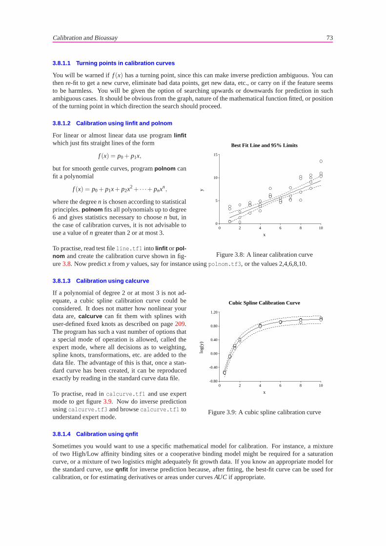
Calibration and Bioassay 73
3.8.1.1 Turning points in calibration curves
You will be warned if f (x) has a turning point, since this can make inverse prediction ambiguous. You canthen re-fit to get a new curve, eliminate bad data points, get new data, etc., or carry on if the feature seemsto be harmless. You will be given the option of searching upwards or downwards for prediction in suchambiguous cases. It should be obvious from the graph, natureof the mathematical function fitted, or positionof the turning point in which direction the search should proceed.
3.8.1.2 Calibration using linfit and polnom
Best Fit Line and 95% Limits
x
y
0
5
10
15
0 2 4 6 8 10
Figure 3.8: A linear calibration curve
For linear or almost linear data use programlinfitwhich just fits straight lines of the form
f (x) = p0 + p1x,
but for smooth gentle curves, programpolnom canfit a polynomial
f (x) = p0 + p1x+ p2x2 + · · ·+ pnxn,
where the degreen is chosen according to statisticalprinciples.polnom fits all polynomials up to degree6 and gives statistics necessary to choosen but, inthe case of calibration curves, it is not advisable touse a value ofn greater than 2 or at most 3.
To practise, read test fileline.tf1 into linfit or pol-nom and create the calibration curve shown in fig-ure3.8. Now predictx from y values, say for instance usingpolnom.tf3 , or the values 2,4,6,8,10.
3.8.1.3 Calibration using calcurve
Cubic Spline Calibration Curve
x
log(
y)
-0.80
-0.40
0.00
0.40
0.80
1.20
0 2 4 6 8 10
Figure 3.9: A cubic spline calibration curve
If a polynomial of degree 2 or at most 3 is not ad-equate, a cubic spline calibration curve could beconsidered. It does not matter how nonlinear yourdata are,calcurve can fit them with splines withuser-defined fixed knots as described on page209.The program has such a vast number of options thata special mode of operation is allowed, called theexpert mode, where all decisions as to weighting,spline knots, transformations, etc. are added to thedata file. The advantage of this is that, once a stan-dard curve has been created, it can be reproducedexactly by reading in the standard curve data file.
To practise, read incalcurve.tf1 and use expertmode to get figure3.9. Now do inverse predictionusingcalcurve.tf3 and browsecalcurve.tf1 tounderstand expert mode.
3.8.1.4 Calibration using qnfit
Sometimes you would want to use a specific mathematical modelfor calibration. For instance, a mixtureof two High/Low affinity binding sites or a cooperative binding model might be required for a saturationcurve, or a mixture of two logistics might adequately fit growth data. If you know an appropriate model forthe standard curve, useqnfit for inverse prediction because, after fitting, the best-fit curve can be used forcalibration, or for estimating derivatives or areas under curvesAUC if appropriate.

74 SIMFIT reference manual: Part 3
3.8.2 Dose response curves, EC50, IC50, ED50, and LD50
A special type of inverse prediction is required when equations are fitted to dose response data in order toestimate some characteristic parameter, such as the half time t1/2, the area under the curveAUC, or me-dian effective dose in bioassay (e.g.ED50, EC50, IC50, LD50, etc.), along with standard errors and 95%confidence limits. The model equations used in this sort of analysis are not supposed to be exact modelsconstructed according to scientific laws, rather they are empirical equations, selected to have a shape that isclose to the shape expected of such data sets. So, while it is is pedantic to insist on using a model based onscientific model building, it is important to select a model that fits closely over a wide variety of conditions.
Older techniques, such as using data subjected to a logarithmic transform in order to fit a linear model, are nolonger called for as they are very unreliable, leading to biased parameter estimates. Hence, in what follows,it is assumed that data are to be analyzed in standard, not logarithmically transformed coordinates, but thereis nothing to prevent data being plotted in transformed space after analysis, as is frequently done when theindependent variable is a concentration, i.e., it is desired to have an the independent variable proportional tochemical potential. The type of analysis called for dependsvery much on the nature of the data, the errordistribution involved, and the goodness of fit of the assumedmodel. It is essential that data are obtained over awide range, and that the best fit curves are plotted and seen tobe free from bias which could seriously degraderoutine estimates of percentiles, say. The only way to decide which of the following procedures should beselected for your data, is to analyze the data using those candidate models that are possibilities, and then toadopt the model that seems to perform best, i.e., gives the closest best fit curves and most sensible inversepredictions.
Exponential modelsIf the data are in the form of a simple or multiphasic exponential decline from a finite value att = 0 tozero ast → ∞, and half timest1/2, or areasAUC are required, useexfit (page59) to fit one or a sum oftwo exponentials with no constant term. Practise withexfit and test fileexfit.tf4 . With the simplemodel
f (t) = Aexp(−kt)
of order 1, then theAUC= A/k andt1/2 = − log(2)/k are given explicitly but, if this model does not fitand a higher model has to be used, then the corresponding parameters will be estimated numerically.
Trapezoidal estimationIf no deterministic model can be used for theAUC it is usual to prefer the trapezoidal method withno data smoothing, where replicates are simply replaced by means values that are then joined up se-quentially by sectional straight lines. The programaverage (page207) is well suited to this sort ofanalysis.
The Hill equationThis empirical equation is
f (x) =Axn
Bn +xn ,
which can be fitted using programinrate (page203), with eithern estimated orn fixed, and it is oftenused in sigmoidal form (i.e.n > 1) to estimate the maximum valueA and half saturation pointB, withsigmoidal data (not data that are only sigmoidal whenx-semilog transformed, as all binding isothermsare sigmoidal inx-semilog space).
Ligand binding and enzyme kinetic models.There are three cases:a) data are increasing as a function of an effector, i.e., ligand or substrate, and the median effectiveligand concentrationED50 or apparentKm = EC50= ED50 is required,b) data are a decreasing function of an inhibitor[I ] at fixed substrate concentration[S] andIC50, theconcentration of inhibitor giving half maximal inhibition, is required, orc) the flux of labelled substrate[Hot], say, is measured as a decreasing function of unlabelled isotope[Cold], say, with[Hot] held fixed.

Calibration and Bioassay 75
If the data are for an increasing saturation curve and ligandbinding models are required, thenhlfit(page63) or, if cooperative effects are present,sffit (page64) can be used to fit one or two binding sitemodels. Practise withsffit andsffit.tf4 .
More often, however, an enzyme kinetic model, such as the Michaelis-Menten equation will be usedas now described. To estimate the maximum rate and apparentKm, i.e., EC50 the equation fitted bymmfit in substrate mode would be
v([S]) =Vmax[S]
Km+[S]
while the interpretation ofIC50 for a reversible inhibitor at concentration[i] with substrate fixed atconcentrationSwould depend on the model assumed as follows.
Competitive inhibitionv([I ]) =Vmax[S]
Km(1+ I/Ki)+ [S]
IC50=Ki(Km+[S])
Km
Uncompetitive inhibitionv([I ]) =Vmax[S]
Km+[S](1+[I ]/Ki]
IC50=Ki(Km+[S])
[S]
Noncompetitive inhibitionv([I ]) =Vmax[S]
(1+[I ]/Ki)(Km+[S])
IC50= Ki
Mixed inhibitionv([I ]) =Vmax[S]
K(1+[I ]/Ki1)+ [S](1+[I ]/Ki2)
IC50=Ki1Ki2(Km+[S])
(KmKi2 +[S]Ki1)
Isotope displacementv([Cold]) =Vmax[Hot]
Km+[Hot]+ [Cold]
IC50= Km+[Hot]
Of course, only two independent parameters can be estimatedwith these models, and, if higher or-der models are required and justified by statistics and graphical deconvolution, the apparentVmax andapparentKm are then estimated numerically.
Growth curves.If the data are in the form of sigmoidal increase, and maximumsize, maximum growth rate, minimumgrowth rate,t1/2 time to half maximum size, etc. are required, then usegcfit in growth curve mode 1(page66). Practise with test filegcfit.tf2 to see how a best-fit model is selected. For instance, withthe logistic model
f (t) =A
1+Bexp(−kt)
t1/2 =log(B)
k
the maximum sizeA and time to reach half maximal sizet/2 are estimated.
Survival curves.If the data are independent estimates of fractions remaining as a function of time or some effector,i.e. sigmoidally decreasing profiles fitted bygcfit in mode 2, andt1/2 is required, then normalize the

76 SIMFIT reference manual: Part 3
data to proportions of time zero values and usegcfit in survival curve mode 2 (page67). Practise withWeibull.tf1 , which has the model equation
S(t) = 1−exp(−(At)B)
t1/2 =log(2)
AB.
Survival time models.If the data are in the form of times to failure, possibly censored, thengcfit should be used in survivaltime mode 3 (page171). Practise with test filesurvive.tf2 . With the previous survival curve andwith survival time models the median survival timet1/2 is estimated, whereZ t1/2
0fT(t)dt =
12,
and fT(t) is the survival probability density function.
Models for proportions.If the data are in the form of numbers of successes (or failures) in groups of known size as a functionof some control variable and you wish to estimate percentiles, e.g.,EC50, IC50, or maybeLD50 (themedian dose for survival in toxicity tests), usegcfit in GLM dose response mode. This is because theerror distribution is binomial, so generalized linear models, as discussed on page50, should be used.You should practise fitting the test fileld50.tf1 with the logistic, probit and log-log models, observingthe goodness of fit options and the ability to change the percentile level interactively. An example ofhow to use this technique follows.
0.00
0.50
1.00
0 2 4 6 8 10
Determination of LD50
Concentration
Pro
port
ion
Fai
ling
0.00
0.50
1.00
0 2 4 6 8 10
Determination of LD50
Concentration
Pro
port
ion
Sur
vivi
ng
Figure 3.10: Plotting LD50 data with error bars
Figure3.10illustrates the determination ofLD50 using GLM. The left hand figure shows the results fromusing the probit model to determineLD50 using test fileld50.tf2 . The right hand figure shows exactly thesame analysis but carried out using the proportion surviving, i.e., the complement of the numbers in test fileld50.tf2 , replacingy, the number failing (dying) in a sample of sizeN, by N− y, the number succeeding(surviving) in a sample of sizeN. Of course the value of theLD50 estimate and the associated standard errorare identical for both data sets. Note that, in GLM analysis,the percentile can be changed interactively, e.g.,if you need to estimateLD25 orLD75, etc.
The left hand figure was created as follows.a) After fitting, the data and best fit curve were transferred into simplot using the[Advanced] option.b) The horizontal line was added interactively by using the[Data] option to add data fory = 0.5 .

Calibration and Bioassay 77
The right hand figure was created as follows.1) After fitting, the best fit curve was added to the project archive using the[Advanced] option to save an
ASCII text coordinate file.2) The data was input into the analysis of proportions procedure described on page123, and the error bar
plot was created.3) The error bar data were transferred tosimplot using the[Advanced] option, then the saved ASCII
text coordinate data for the best fit curve and line aty = 0.5 were added interactively using the[Data]option.
The point about about using the analysis of proportions routines in this way for the error bars in the righthand figure is that exact, unsymmetrical 95% confidence limits can be generated from the sample sizes andnumbers of successes in this way.
3.8.3 95% confidence regions in inverse prediction
polnom estimates non-symmetrical confidence limits assuming thattheN values ofy for inverse predictionand weights supplied for weighting are exact, and that the model fitted hasn parameters that are justifiedstatistically. calcurve uses the weights supplied, or the estimated coefficient of variation, to fit confidenceenvelope splines either side of the best fit spline, by employing an empirical technique developed by sim-ulation studies. Root finding is employed to locate the intersection of theyi supplied with the envelopes.The AUC, LD50, half-saturation, asymptote and other inverse predictions in SIMFIT use at distribution withN−n degrees of freedom, and the variance-covariance matrix estimated from the regression. That is, assum-ing a prediction parameter defined byp = f (θ1,θ2, . . . ,θn), a central 95% confidence region is constructedusing the prediction parameter variance estimated by
V(p) =n
∑i=1
(
∂ f∂θi
)2
V(θi)+2n
∑i=2
i−1
∑j=1
∂ f∂θi
∂ f∂θ j
CV(θi ,θ j).

78 SIMFIT reference manual: Part 3
3.9 Statistics
The main part of the SIMFIT statistics functions are to be found in the programsimstat , which is in manyways like a small scale statistics package. This provides options for data exploration, statistical tests, analysisof variance, multivariate analysis, regression, time series, power calculations, etc., as well as a number ofcalculations, like finding zeros of polynomials, or values of determinants, inverses, eigenvalues or eigenvaluesof matrices. In addition tosimstat there are also several specialized programs that can be usedfor moredetailed work and to obtain information about dedicated statistical distributions and related tests but, beforedescribing thesimstat procedures with worked examples, a few comments about testsmay be helpful.
3.9.1 Tests
A test statistic is a function evaluated on a data set, and thesignificance level of a test is the probability ofobtaining a test statistic as extreme, or more extreme, froma random sample, given a null hypothesisH0,which usually specifies a distribution for that test statistic. If the error rate, i.e. significance levelp is lessthan some critical level, sayα = 0.05 orα = 0.01, it is reasonable to consider whether the null hypothesisshould be rejected. The correct procedure is to choose a test, decide whether to use the upper, lower, ortwo-tail test statistic as appropriate, select the critical significance level, do the test, then accept the outcome.What is not valid is to try several tests until you find one thatgives you the result you want. That is becausethe probability of a Type 1 error increases monotonically asthe number of tests increases, particularly if thetests are on the same data set, or some subsets of a larger dataset. This multiple testing should never bedone, but everybody seems to do it. Of course, all bets are offanyway if the sample does not conform to theassumptions implied byH0, for instance, doing at test with two samples that are known not to be normallydistributed with the same variance.
3.9.2 Multiple tests
Statistical packages are designed to be used in the rather pedantic but correct manner just described, whichmakes them rather inconvenient for data exploration. SIMFIT, on the other hand, is biased towards dataexploration, so that various types of multiple testing can be done. However, once the phase of data explorationis completed, there is nothing to stop you making the necessary decisions and only using the subset of resultscalculated by the SIMFIT statistical programs, as in the classical (correct) manner. Take, for example, thettest. SIMFIT does a test for normality and variance equality on the two samples supplied, it reports lower,upper and two tail test statistics andp values simultaneously, it performs a corrected test for thecase ofunequal variances at the same time, it allows you to follow the t test by a pairedt test if the sample sizes areequal and, after doing thet test, it saves the data for a Mann-Whitney U or Kolmogorov-Smirnov 2-sampletest on request. An even more extreme example is the all possible pairwise comparisons option, which doesall possiblet, Mann-Whitney U and Kolmogorov-Smirnov2-sample tests on alibrary file of column vectors.
In fact there are two ways to view this type of multiple testing. If you are just doing data exploration toidentify possible differences between samples, you can just regard thep values as a measure of the differencesbetween pairs of samples, in that smallp values indicate samples which seem to have different distributions.In this case you would attach no importance as to whether thep values are less than any supposed criticalαvalues. On the other hand, if you are trying to identify samples that differ significantly, then some technique isrequired to structure the multiple testing procedure and/or alter the significance level, as in the Tukey Q test.If the experimentwise error rate isαe while the comparisonwise error rate isαc and there arek comparisons
then, from equating the probability ofk tests with no Type 1 errors it follows that
1−αe = (1−αc)k.
This is known as the Dunn-Sidak correction, but, alternatively, the Bonferroni correction is based on therecommendation that, fork tests, the error rate should be decreased fromα to α/k, which gives a similarvalue to use forαc in the multiple test, givenαe.

Data exploration 79
3.9.3 Data exploration
SIMFIT has a number of techniques that are appropriate for exploration of data and data mining. Suchtechniques do not always lead to meaningful hypothesis tests, but are best used for preliminary investigationof data sets prior to more specific model building.
3.9.3.1 Exhaustive analysis: arbitrary vector
This procedure is used when you have a single sample (column vector) and wish to explore the overallstatistical properties of the data. For example, read in thevector test filenormal.tf1 and you will see that allthe usual summary statistics are calculated as in Table3.18, including the range, hinges (i.e. quartiles), mean
Data: 50 numbers from a normal distribution mu = 0 and sigma = 1Sample size 50Minimum, Maximum values -2.208E+00, 1.617E+00Lower and Upper Hinges -8.550E-01, 7.860E-01Coefficient of skewness -1.602E-02Coefficient of kurtosis -8.551E-01Median value -9.736E-02Sample mean -2.579E-02Sample standard deviation 1.006E+00: CV% = 3.899E+03%Standard error of the mean 1.422E-01Upper 2.5% t-value 2.010E+00Lower 95% con lim for mean -3.116E-01Upper 95% con lim for mean 2.600E-01Variance of the sample 1.011E+00Lower 95% con lim for var. 7.055E-01Upper 95% con lim for var. 1.570E+00Shapiro-Wilks W statistic 9.627E-01Significance level for W 0.1153 Tentatively accept normali ty
Table 3.18: Exhaustive analysis of an arbitrary vector
x, standard deviations, and the normalized sample momentss3 (coefficient of skewness), ands4 (coefficientof kurtosis), defined in a sample of sizen by
x =n
∑i=1
xi/n
s=
√
n
∑i=1
(xi − x)2/(n−1)
s3 =n
∑i=1
(xi − x)3/[(n−1)s3]
s4 =n
∑i=1
(xi − x)4/[(n−1)s4]−3.
You can then do a Shapiro-Wilks test for normality (which will, of course, not always be appropriate) or cre-ate a histogram, pie chart, cumulative distribution plot orappropriate curve-fitting files. This option is a veryvaluable way to explore any single sample before considering other tests. If you created filesvector.1standvector.2nd as recommended earlier you can now examine these. Note that once a sample has been readinto programsimstat it is saved as the current sample for editing, transforming or re-testing Since vectorshave only one coordinate, graphical display requires a further coordinate. In the case of histograms the extracoordinate is provided by the choice of bins, which dictatesthe shape, but in the case of cumulative distribu-tions it is automatically created as steps and therefore of unique shape. Pie chart segments are calculated in

80 SIMFIT reference manual: Part 3
proportion to the sample values, which means that this is only appropriate for positive samples, e.g., counts.The other techniques illustrated in figure3.11 require further explanation. If the sample values have been
-3.00
-2.00
-1.00
0.00
1.00
2.00
0 10 20 30 40 50
Vector Plotted as a Time Series
Position
Val
ues
-3.00
-2.00
-1.00
0.00
1.00
2.00
0 10 20 30 40 50
Vector Plotted as Zero Centred Rods
Position
Val
ues
0.00
1.00
2.00
3.00
0.00 1.00 2.00 3.00
Vector Plotted in Half Normal Format
Expected Half-Normal Order Statistic
Ord
ered
Abs
olut
e V
alue
s
-2.50
-1.25
0.00
1.25
2.50
-2.50 -1.25 0.00 1.25 2.50
Vector Plotted in Normal Format
Expected Normal Order Statistic
Ord
ered
Val
ues
Figure 3.11: Plotting vectors
measured in some sequence of time or space, then they values could be the sample values while thex valueswould be successive integers, as in the time series plot. Sometimes it is useful to see the variation in thesample with respect to some fixed reference value, as in the zero centered rods plot. The data can be centeredautomatically about zero by subtracting the sample mean if this is required. The half normal and normal plotsare particularly useful when testing for a normal distribution with residuals, which should be approximatelynormally distributed if the correct model is fitted. In the half normal plot, the absolute values of a sample ofsizen are first ordered then plotted asyi , i = 1, . . . ,n, while the half normal order statistics are approximatedby
xi = Φ−1
(
n+ i + 12
2n+ 98
)
, i = 1, . . . ,n
which is valuable for detecting outliers in regression. Thenormal scores plot simply uses the ordered sampleasy and the normal order statistics are approximated by
xi = Φ−1
(
i − 38
n+ 14
)
, i = 1, . . . ,n
which makes it easy to visualize departures from normality.Best fit lines, correlation coefficients, and signif-icance values are also calculated for half normal and normalplots. Note that a more accurate calculation forexpected values of normal order statistics is employed whenthe Shapiro-Wilks test for normality (page89)is used and a normal scores plot is required.

Data exploration 81
3.9.3.2 Exhaustive analysis: arbitrary matrix
This procedure is provided for when you have recorded several variables (columns) with multiple cases (rows)and therefore have data in the form of a rectangular matrix, as with Table3.19 resulting from analyzingmatrix.tf2 . The option is used when you want summary statistics for a numerical matrix with no missing
Data: Matrix of order 7 by 5Row Mean Variance St.Dev. Coeff.Var.
1 3.6800E+00 8.1970E+00 2.8630E+00 77.80%2 6.8040E+00 9.5905E+00 3.0969E+00 45.52%3 6.2460E+00 3.5253E+00 1.8776E+00 30.06%4 4.5460E+00 7.1105E+00 2.6666E+00 58.66%5 5.7840E+00 5.7305E+00 2.3939E+00 41.39%6 4.8220E+00 6.7613E+00 2.6003E+00 53.92%7 5.9400E+00 1.7436E+00 1.3205E+00 22.23%
Table 3.19: Exhaustive analysis of an arbitrary matrix
values. It analyzes every row and column in the matrix then, on request, exhaustive analysis of any chosenrow or column can be performed, as in exhaustive analysis of avector.
Often the rows or columns of a data matrix have pairwise meaning. For instance, two columns may be mea-surements from two populations where it is of interest if thepopulations have the same means. If the popula-tions are normally distributed with the same variance, thenan unpairedt test might be appropriate (page90),otherwise the corresponding nonparametric test (Mann-Whitney U, page95), or possibly a Kolmogorov-Smirnov 2-sample test (page93) might be better. Again, two columns might be paired, as withmeasurementsbefore and after treatment on the same subjects. Here, if normality of differences is reasonable, a pairedttest (page92) might be called for, otherwise the corresponding nonparametric procedure (Wilcoxon signedrank test, page96), or possibly a run test (page103), or a sign test (page102) might be useful for testing forabsence of treatment effect. Table3.20illustrates the option to do statistics on paired rows or columns, in thiscase columns 1 and 2 ofmatrix.tf2 . You identify two rows or columns from the matrix then simpleplots,linear regression, correlation, and chosen statistical tests can be done. Note that all thep values calculatedfor this procedure are for two-tail tests, while the run, Wilcoxon sign rank, and sign test ignore values whichare identical in the two columns. More detailed tests can be done on the selected column vectors by thecomprehensive statistical test options to be discussed subsequently (page87).
The comprehensive analysis of a matrix procedure also allows for the data matrix to be plotted as a 2-dimensional bar chart, assuming that the rows are cases and the columns are numbers in distinct categories,or as a 3-dimensional bar chart assuming that all cell entries are as in a contingency table, or similar. Alterna-tively, plots displaying the columns as scattergrams, box and whisker plots, or bar charts with error bars canbe constructed.
3.9.3.3 Exhaustive analysis: multivariate normal matrix
This provides options that are useful before proceeding to more specific techniques that depend on multivari-ate normality (page279), e.g., MANOVA and some types of ANOVA.
A graphical technique is provided for investigating if a data matrix with n rows andm columns, wheren >> m> 1, is consistent with a multivariate normal distribution. For example, figure3.12 shows plots fortwo random samples from a multivariate normal distribution. The plot uses the fact that, for a multivariatenormal distribution with sample mean ¯x and sample covariance matrixS,
(x− x)TS−1(x− x) ∼ m(n2−1)
n(n−m)Fm,n−m,

82 SIMFIT reference manual: Part 3
Unpaired t test:t = -3.094E+00p = 0.0093 *p =< 0.01Paired t test:t = -3.978E+00p = 0.0073 *p =< 0.01Kolmogorov-Smirnov 2-sample test:d = 7.143E-01z = 3.818E-01p = 0.0082 *p =< 0.01Mann-Whitney U test:u = 7.000E+00z = -2.172E+00p = 0.0262 *p =< 0.05Wilcoxon signed rank test:w = 1.000E+00z = -2.113E+00p = 0.0313 *p =< 0.05Run test:+ = 1 (number of x > y)- = 6 (number of x < y)p = 0.2857Sign test:N = 7 (non-tied pairs)- = 6 (number of x < y)p = 0.1250
Table 3.20: Statistics on paired columns of a matrix
0.00
0.20
0.40
0.60
0.80
1.00
0.00 2.00 4.00 6.00
Multivariate Plot: r = 0.754
F-quantiles
Ran
ked
Tra
nsfo
rms
n = 8, m = 4
0.00
1.00
2.00
3.00
0.00 1.00 2.00 3.00 4.00
Multivariate Plot: r = 0.980
F-quantiles
Ran
ked
Tra
nsfo
rms
n = 20, m = 4
Figure 3.12: Plot to diagnose multivariate normality
wherex is a further independent observation from this population,so that the transforms plotted againstthe quantiles of anF distribution withm andn−m degrees of freedom, i.e. according to the cumulativeprobabilities for(i −0.5)/n for i = 1,2, . . . ,n should be a straight line. It can be seen from figure3.12thatthis plot is of little value for small values ofn, sayn ≈ 2m but becomes progressively more useful as thesample size increases, sayn > 5m.
Again, there are procedures to calculate the column means ¯x j , andm by m sample covariance matrixS,

Data exploration 83
defined for an by m data matrixxi j with n≥ 2,m≥ 2 as
x j =1n
n
∑i=1
xi j
sjk =1
n−1
n
∑i=1
(xi j − x j)(xik − xk)
and then exploit several techniques which use these estimates for the population mean vector and covariancematrix. The eigenvalues and determinants of the sample covariance matrix and its inverse are required forseveral MANOVA techniques, so these can also be estimated. It is possible to perform two variants of theHotellingT2 test, namely
• testing for equality of the mean vector with a specified reference vector of means, or
• testing for equality of all means without specifying a reference mean.
Dealing first with testing that a vector of sample means is consistent with a reference vector, table3.21resulted when the test filehotel.tf1 was analyzed using the Hotelling one sample test procedure.This tests
Hotelling one sample T-square test
H0: Delta = (Mean - Expected) are all zero
No. rows = 10, No. columns = 4Hotelling T-square = 7.439E+00F Statistic (FTS) = 1.240E+00Deg. Free. (d1,d2) = 4, 6P(F(d1,d2) >= FTS) = 0.3869Column Mean Std.Err. Expected Delta t p
1 -5.300E-01 4.63E-01 0.00E+00 -5.30E-01 -1.15E+00 0.28152 -3.000E-02 3.86E-01 0.00E+00 -3.00E-02 -7.78E-02 0.93973 -5.900E-01 4.91E-01 0.00E+00 -5.90E-01 -1.20E+00 0.26014 3.100E+00 1.95E+00 0.00E+00 3.10E+00 1.59E+00 0.1457
Table 3.21: HotellingT2 test forH0: means = reference
the null hypothesisH0 : µ = µ0 against the alternativeH1 : µ 6= µ0, whereµ0 is a known mean vector and noassumptions are made about the covariance matrixΣ. Hotelling’sT2 is
T2 = n(x−µ0)TS−1(x−µ0)
and, if H0 is true, then anF test can be used since(n−m)T2/(m(n− 1)) is distributed asymptotically asFm,n−m. Users can input any reference mean vectorµ0 to test for equality of means but, when the data columnsare all differences between two observations for the same subjects and the aim is to test for no significantdifferences, so thatµ0 is the zero vector, as withhotel.tf1 , the test is a sort of higher dimensional analogueof the pairedt test. Table3.21also shows the results whent tests are applied to the individual columns ofdifferences between the sample means ¯x and the reference meansµ0, which is suspect because of multipletesting but, in this case, the conclusion is the same as the Hotelling T2 test: none of the column means aresignificantly different from zero.
Now, turning to a test that all means are equal, table3.22shows the results when the data inanova6.tf1 areanalyzed, and the theoretical background to this test will be presented subsequently (page119).
Options are provided for investigating the structure of thecovariance matrix. The sample covariance matrixand its inverse can be displayed along with eigenvalues and determinants, and there are also options to checkif the covariance matrix has a special form, namely

84 SIMFIT reference manual: Part 3
Hotelling one sample T-square test
H0: Column means are all equal
No. rows = 5, No. columns = 4Hotelling T-square = 1.705E+02F Statistic (FTS) = 2.841E+01Deg. Free. (d1,d2) = 3, 2P(F(d1,d2) >= FTS) = 0.0342 Reject H0 at 5% sig.level
Table 3.22: HotellingT2 test forH0: means are equal
• testing for compound symmetry,
• testing for spherical symmetry, and
• testing for spherical symmetry of the covariance matrix of orthonormal contrasts.
For instance, using the test filehotel.tf1 produces the results of table3.23 showing an application of a testfor compound symmetry and a test for sphericity. Compound symmetry is when a covariance matrixΣ has aspecial form with constant nonnegative diagonals and equalnonnegative off-diagonal elements as follows.
Σ = σ2
1 ρ . . . ρρ 1 . . . ρ. . . . . . . . . . . .ρ ρ . . . 1
This can be tested using estimates for the diagonal and off-diagonal elementsσ2 andσ2ρ as follows
s2 =1m
m
∑i=1
sii
s2r =2
m(m−1)
m
∑i=2
i−1
∑j=1
si j .
The Wilks generalized likelihood-ratio statistic is
L =|S|
(s2−s2r)m−1[s2 +(m−1)s2r],
where the numerator is the determinant of the covariance matrix estimated withν degrees of freedom, whilethe denominator is the determinant of the matrix with average variance on the diagonals and average covari-ance as off-diagonal elements, and this is used to constructthe test statistic
χ2 = −[
ν− m(m+1)2(2m−3)
6(m−1)(m2+m−4)
]
logL
which, for largeν, has an approximate chi-squared distribution withm(m+1)/2−2 degrees of freedom.
The sphericity test, designed to test the null hypothesisH0 : Σ = kI againstH1 : Σ 6= kI. In other words, thepopulation covariance matrixΣ is a simple multiple of the identity matrix, which is a central requirementfor some analytical procedures. If the sample covariance matrix Shas eigenvaluesαi for i = 1,2, . . . ,m then,defining the arithmetic meanA and geometric meanG of these eigenvalues as
A = (1/m)m
∑i=1
αi
G = (m
∏i=1
αi)1/m,

Data exploration 85
Variance-Covariance matrix2.1401E+00 -1.1878E-01 -8.9411E-01 3.5922E+00
-1.1878E-01 1.4868E+00 7.9144E-01 1.8811E+00-8.9411E-01 7.9144E-01 2.4099E+00 -4.6011E+00
3.5922E+00 1.8811E+00 -4.6011E+00 3.7878E+01Pearson product-moment correlations
1.0000 -0.0666 -0.3937 0.3990-0.0666 1.0000 0.4181 0.2507-0.3937 0.4181 1.0000 -0.4816
0.3990 0.2507 -0.4816 1.0000
Compound symmetry test
H0: Covariance matrix has compound symmetry
No. of groups = 1No. of variables (k) = 4Sample size (n) = 10Determinant of CV = 9.814E+01Determinant of S_0 = 1.452E+04LRTS (-2*log(lambda)) = 3.630E+01Degrees of Freedom = 8P(chi-square >= LRTS) = 0.0000 Reject H0 at 1% sig.level
Likelihood ratio sphericity test
H0: Covariance matrix = k*Identity (for some k > 0)
No. small eigenvalues = 0 (i.e. < 1.00E-07)No. of variables (k) = 4Sample size (n) = 10Determinant of CV = 9.814E+01Trace of CV = 4.391E+01Mauchly W statistic = 6.756E-03LRTS (-2*log(lambda)) = 4.997E+01Degrees of Freedom = 9P(chi-square >= LRTS) = 0.0000 Reject H0 at 1% sig.level
Table 3.23: Covariance matrix symmetry and sphericity tests
the likelihood ratio test statistic−2logλ = nmlog(A/G)
is distributed asymptotically asχ2 with (m−1)(m+2)/2 degrees of freedom. Using the fact that the deter-minant of a covariance matrix is the product of the eigenvalues while the trace is the sum, the Mauchly teststatisticW can also be calculated fromA andG since
W =|S|
Tr(S)/mm
=∏m
i=1αi
(∑mi=1αi)/mm
so that−2logλ = −nlogW.
Clearly, the test rejects the assumption that the covariance matrix is a multiple of the identity matrix in this

86 SIMFIT reference manual: Part 3
case, a conclusion which is obvious from inspecting the sample covariance and correlation matrices. Sincethe calculation of small eigenvalues is very inaccurate when the condition number of the covariance matrix isappreciable, any eigenvalues less than the minimal threshold indicated are treated as equal to that thresholdwhen calculating the test statistic.
3.9.3.4 All possible pairwise tests ( n vectors or a library file)
This option is used when you have several samples (column vectors) and wish to explore which samplesdiffer significantly. The procedure takes in a library file referencing sets of vector files and then performs anycombination of two-tailedt, Kolmogorov-Smirnov 2-sample, and/or Mann-Whitney U tests on all possiblepairs. It is usual to select either justt tests for data that you know to be normally distributed, or just Mann-WhitneyU tests otherwise. Because the number of tests is large, e.g.,3n(n−1)/2 for all tests withn samples,be careful not to use it with too many samples.
For example, try it by reading in the library filesanova1.tfl (or the smaller data setnpcorr.tfl with threevectors of length 9 where the results are shown in table3.24) and observing that significant differences are
Mann-Whitney-U/Kolmogorov-Smirnov-D/unpaired-t tests
No. tests = 9, p(1%) = 0.001111, p(5%) = 0.005556 [Bonferroni ]column2.tf1 (data set 1)column2.tf2 (data set 2)N1 = 9, N2 = 9, MWU = 8.000E+00, p = 0.00226 *
KSD = 7.778E-01, p = 0.00109 **T = -3.716E+00, p = 0.00188 *
column2.tf1 (data set 1)column2.tf3 (data set 3)N1 = 9, N2 = 9, MWU = 2.100E+01, p = 0.08889
KSD = 5.556E-01, p = 0.05545T = -2.042E+00, p = 0.05796
column2.tf2 (data set 2)column2.tf3 (data set 3)N1 = 9, N2 = 9, MWU = 5.550E+01, p = 0.19589
KSD = 4.444E-01, p = 0.20511T = 1.461E+00, p = 0.16350
Table 3.24: All possible comparisons
highlighted. This technique can be very useful in preliminary data analysis, for instance to identify potentiallyrogue columns in analysis of variance, i.e., pairs of columns associated with smallp values. However, it isup to you to appreciate when the results are meaningful and tomake the necessary adjustment to criticalsignificance levels where the Bonferroni principle is required (due to multiple tests on the same data).

Statistical tests 87
3.9.4 Statistical tests
3.9.4.1 1-sample t test
This procedure is used when you have a sample that is known to be normally distributed and wish to testH0: the mean isµ0, whereµ0 is a known quantity. Table3.25shows the results for such a 1-samplet test on
No. of x-values = 50No. of degrees of freedom = 49Theoretical mean (mu_0) = 0.000E+00Sample mean (x_bar) = -2.579E-02Std. err. of mean (SE) = 1.422E-01TS = (x_bar - mu_0)/SE = -1.814E-01P(t >= TS) (upper tail p) = 0.5716P(t =< TS) (lower tail p) = 0.4284p for two tailed t test = 0.8568Diffn. D = x_bar - x_mu = -2.579E-02Lower 95% con. lim. for D = -3.116E-01Upper 95% con. lim. for D = 2.600E-01Conclusion: Consider accepting equality of means
Table 3.25: One samplet test
the data in test filenormal.tf1 . The procedure can first do a Shapiro-Wilks test for normality (page89) ifrequested and then, forn values ofxi , it calculates the sample mean ¯x, sample variances2, standard error ofthe meansx and test statisticTSaccording to
x =1n
n
∑i=1
xi
s2 =1
n−1
n
∑i=1
(xi − x)2
sx =√
s2/n
TS=x−µ0
sx
whereµ0 is the supposed theoretical, user-supplied population mean. The significance levels for upper, lower,and two-tailed tests are calculated for at distribution withn−1 degrees of freedom. You can then changeµ0
or select a new data set.
3.9.4.2 1-sample Kolmogorov-Smirnov test
This nonparametric procedure is used when you have a single sample (column vector) of reasonable size (saygreater than 20) and wish to explore if it is consistent with some known distribution, e.g., normal, binomial,Poisson, gamma, etc. The test only works optimally with large samples where the null distribution is acontinuous distribution that can be specified exactly and not defined using parameters estimated from thesample. It calculates the maximum positive differenceD+
n , negative differenceD−n , and overall difference
Dn = maximum ofD+n andD−
n between the sample cumulative distribution functionS(xi) and the theoretical

88 SIMFIT reference manual: Part 3
cdf F(xi) underH0, i.e., if frequenciesf (xi) are observed for the variablexi in a sample of sizen, then
S(xi) =i
∑j=1
f (x j )/n
F(xi) = P(x≤ xi)
D+n = max(S(xi)−F(xi),0), i = 1,2, . . . ,n
D−n = max(F(xi)−S(xi−1),0), i = 2,3, . . . ,n
Dn = max(D+n ,D−
n ).
The standardized statisticsZ = D√
n are calculated for theD values appropriate for upper-tail, lower-tail,or two-tailed tests, then the exact significance levels are calculated by SIMFIT for small samples by solvingP(Dn ≤ a/n) using the difference equation
[2a]
∑j=0
(−1) j((2a− j) j/ j!)qr− j(a) = 0, r = 2[a]+1,2[a]+2, . . .
with initial conditions
qr(a) = 1, r = 0
= r r/r!, r = 1, . . . , [a]
= r r/r! −2a[r−a]
∑j=0
((a+ j) j−1/ j!)(r −a− j)r− j/(r − j)!, r = [a+1], . . . ,2[a],
where[a] is the largest integer≤ a regardless of the sign ofa, while the series
limn→∞
P
(
Dn ≤z√n
)
= 1−2∞
∑i=1
(−1)i−1exp(−2i2z2)
is used for large samples. For example, input the filenormal.tf1 and test to see if these numbers do comefrom a normal distribution. See if your own filesvector.1st andvector.2nd come from a uniform or abeta distribution. Note that there are two ways to perform this test; you can state the parameters, or they canbe estimated by the program from the sample, using the methodof moments, or else maximum likelihood.However, calculating parameters from samples compromisesthis test leading to a significant reduction in
power. If you want to see if a sample comes from a binomial, Poisson, uniform, beta, gamma, lognormalnormal, or Weibull distribution, etc., the data supplied must be of a type that is consistent with the supposeddistribution, otherwise you will get error messages. Before you do any parametric test with a sample, you canalways use this option to see if the sample is in fact consistent with the supposed distribution. An extremelyvaluable option provided is to view the best-fitcdf superimposed upon the sample cumulative distribution,which is a very convincing way to assess goodness of fit. Superposition of the best fitpdf on the samplehistogram can also be requested, which is useful for discrete distributions but less useful for continuousdistributions, since it requires large samples (say greater than 50) and the histogram shape depends on thenumber of bins selected. Table3.26 illustrates the results when the test filenormal.tf1 is analyzed tosee if the data are consistent with a normal distribution using the Kolmogorov-Smirnov test with parametersestimated from the sample, and the Shapiro-Wilks test to be described shortly (page89). Note that typicalplots of the best fit normal distribution with the sample cumulative distribution, and best-fit density functionoverlayed on the sample histogram obtained using this procedure can be seen on page22, while normal scoresplots were discussed and illustrated on page80. Note that significance levels are given in the table for upper-tail, lower-tail, and two-tail tests. In general you shouldonly use the two-tail probability levels, reservingthe one-tail tests for situations where the only possibility is either that the sample mean may be shifted to theright of the null distribution requiring an upper-tail test, or to the left requiring a lower-tail test

Statistical tests 89
Data: 50 numbers from a normal distribution mu = 0 and sigma = 1Parameters estimated from sample are:mu = -2.579E-02, se = 1.422E-01, 95%cl = ( -3.116E-01, 2.600E -01)sigma = 1.006E+00, sigmaˆ2 = 1.011E+00, 95%cl = (7.055E-01, 1.570E+00)Sample size = 50, i.e. no. of x-values
H0: F(x) equals G(y) (x & theory are comparable) againstH1: F(x) not equal to G(y) (x & theory not comparable)D = 9.206E-02z = 6.510E-01p = 0.7559H2: F(x) > G(y) (x tend to be smaller than theoretical)D = 9.206E-02z = 6.510E-01p = 0.3780H3: F(x) < G(y) (x tend to be larger than theoretical)D = 6.220E-02z = 4.398E-01p = 0.4919Shapiro-Wilks normality test:W statistic = 9.627E-01Sign. level = 0.1153 Tentatively accept normality
Table 3.26: Kolomogorov-Smirnov 1-sample and Shapiro-Wilks tests
3.9.4.3 1-sample Shapiro-Wilks test for normality
This procedure is used when you have data and wish to testH0: the sample is normally distributed. Itis a very useful general test which may perform better than the Kolmogorov-Smirnov 1-sample test justdescribed, but the power is low, so reasonably large sample sizes (say> 20) are required. The test statisticW,where 0≤W ≤ 1, is constructed by considering the regression of ordered sample values on the correspondingexpected normal order statistics, so a normal scores plot should always be examined when testing for a normaldistribution, and it should be approximately linear if a sample is from a normal distribution. For a sample ofsizen, this plot and the theory for the Shapiro-Wilks test, require the normal scores, i.e., the expected valuesof therth largest order statistics given by
E(r,n) =n!
(r −1)!(n− r)!
Z ∞
−∞x[1−Φ(x)]r−1[Φ(x)]n−rφ(x)dx,
whereφ(x) =1√2π
exp
(
−12
x2)
,
andΦ(x) =
Z x
−∞φ(u)du.
Then the test statisticW uses the vector of expected values of a standard normal samplex1,x2, . . . ,xn and thecorresponding covariance matrix, that is
mi = E(xi) (i = 1,2, . . . ,n),
andvi j = cov(xi ,x j) (i, j = 1,2, . . . ,n),

90 SIMFIT reference manual: Part 3
so that, for an ordered random sampley1,y2, . . . ,yn,
W =
(
n
∑i=1
aiyi
)2
n
∑i=1
(yi − y)2,
whereaT = mTV−1[(mTV−1)(V−1m)]−12 .
Finally, the significance level for the statisticW calculated from a sample is obtained by transformation to anapproximately standard normal deviate using
z=(1−W)λ −µ
σ,
whereλ is estimated from the sample andµ, andσ are the sample mean and standard deviation. Values ofWclose to 1 support normality, while values close to 0 suggestdeviation from normality.
3.9.4.4 1-sample Dispersion and Fisher exact Poisson tests
This procedure is used when you have data in the form of non-negative integers (e.g. counts) and wish totestH0: the sample is from a Poisson distribution. Given a sample ofn observationsxi with sample meanx = ∑n
i=1xi/n from a Poisson distribution (page277), the dispersionD given by
D =n
∑i=1
(xi − x)2/x
is approximately chi-square distributed withn−1 degrees of freedom. A test for consistency with a Poissondistribution can be based on thisD statistic but, with small samples, the more accurate Fisherexact test canbe performed. This estimates the probability of the sample observed based on all partitions consistent withthe sample mean, size and total. After performing these tests on a sample of nonnegative integers, this optionthen plots a histogram of the observed and expected frequencies (page249). Table3.27shows the resultsfrom analyzing data in the test filepoisson.tf1 and also the results from using the previously discussedKolmogorov 1-sample test with the same data. Clearly the data are consistent with a Poisson distribution.The mean and expectation of a Poisson distribution are identical and three cases can arise.
1. The sample variance exceeds the upper confidence limit forthe sample mean indicating over-dispersion, i.e. too much clustering/clumping.
2. The sample variance is within the confidence limits for thesample mean indicating consistency with aPoisson distribution.
3. The sample variance is less than the lower confidence limitfor the sample mean indicating under-dispersion, i.e. too much uniformity.
Output from the Kolmogorov-Smirnov 1-sample test for a Poisson distribution indicates if the variance issuspiciously small or large.
3.9.4.5 2-sample unpaired t and variance ratio tests
This procedure is used when you have two samplesx = (x1,x2, . . . ,xm) and y = (y1,y2, . . . ,yn) (i.e., twocolumn vectors of measurements, not counts) which are assumed to come from two normal distributions withthe same variance, and you wish to testH0: the means of the two samples are equal. It is equivalent to 1-way

Statistical tests 91
Dispersion and Fisher-exact Poisson testsSample size = 40Sample total = 44Sample ssq = 80Sample mean = 1.100E+00Lower 95% con.lim. = 7.993E-01Upper 95% con.lim. = 1.477E+00Sample variance = 8.103E-01Dispersion (D) = 2.873E+01P(Chi-sq >= D) = 0.88632No. deg. freedom = 39Fisher exact Prob. = 0.91999
Kolmogorov-Smirnov one sample testH0: F(x) equals G(y) (x & theory are comparable) againstH1: F(x) not equal to G(y) (x & theory not comparable)D = 1.079E-01z = 6.822E-01p = 0.7003H2: F(x) > G(y) (x tend to be smaller than theoretical)D = 7.597E-02z = 4.805E-01p = 0.4808H3: F(x) < G(y) (x tend to be larger than theoretical)D = 1.079E-01z = 6.822E-01p = 0.3501
Table 3.27: Poisson distribution tests
analysis of variance (page110) with just two columns. The test statisticU that is calculated is
U =x− y
√
s2p
(
1m
+1n
)
,
wherex =m
∑i=1
xi/m,
y =n
∑i=1
yi/n,
s2x =
m
∑i=1
(xi − x)2/(m−1),
s2y =
n
∑i=1
(yi − y)2/(n−1),
ands2p =
(m−1)s2x +(n−1)s2
y
m+n−2,
so thats2p is the pooled variance estimate andU has at distribution with m+ n− 2 degrees of freedom
underH0: the means are identical. The two sample means and sample variances are calculated, then thetest statistic is calculated and the significance levels fora lower, upper and two-tail test are calculated. Forexample, read in the test file pairsttest.tf2 and ttest.tf3 and then, after analyzing them, read in thetest file pairsttest.tf4 and ttest.tf5 . Note that before doing at or pairedt test, the program checks,
92 SIMFIT reference manual: Part 3
using a Shapiro-Wilks test, to see if the samples are consistent with normal distributions, and it also does avariance ratio test to see if the samples have common variances. However, note that the Shapiro-Wilks test,which examines the correlation between the sample cumulative distribution and the expected order statisticsfor normal distributions, and also theF test for common variances, which calculatesF given by
F = max
(
s2x
s2y,s2y
s2x
)
and compares this to critical values for the appropriateF distribution, are very weak with small samples, sayless than 25. So you should not do these tests with small samples but, if you have large samples which donot pass these tests, you should ask yourself if doing at test makes sense (since at test depends upon theassumption that both samples are normal and with the same variance).
Note that the Satterthwaite procedure, using atc statistic withν degrees of freedom calculated with the Welchcorrection for unequal variances is performed at the same time, using
tc =x− y
se(x− y)
se(x− y) =
√
s2x
m+
s2y
n
ν =se(x− y)4
(s2x/m)2/(m−1)+ (s2
y/n)2/(n−1)
and the results are displayed within square brackets adjacent to the uncorrected results. However, this shouldonly be trusted if the data sets seem approximately normallydistributed with fairly similar variances. Notethat, every time SIMFIT estimates parameters by regression, it estimates the parameter standard error anddoes at test for parameter redundancy. However, at any time subsequently, you can choose the option tocompare two parameters and estimated standard errors from the curve fitting menus, which does the abovetest corrected for unequal variances. Table3.28shows the results from analyzing data inttest.tf4 andttest.tf5 which are not paired. Clearly the correction for unequal variance is unimportant in this case andthe unpairedt test supports equality of the means. Note that, if data have been input from files,simstat savesthe last set of files for re-analysis, for instance to do the next test.
3.9.4.6 2-sample paired t test
This procedure is used when you have paired measurements, e.g., two successive measurements on the samesubjects before and after treatments, and wish to testH0: the mean of the differences between paired mea-surements is zero. Just as the unpairedt test is equivalent to analysis of variance with just two columns,the pairedt test is equivalent to repeated measurements analysis of variance. For convenience, data for allpaired tests also can be input as an by 2 matrix rather than two vectors of lengthn. The pairedt test is basedon the assumption that the differences between corresponding pairsxi andyi are normally distributed, notnecessarily the original data although this would normallyhave to be the case, and it requires the calculationof d, s2
d, andtd given by
di = xi −yi
d =n
∑i=1
di/n
s2d =
n
∑i=1
(di − d)2/(n−1)
td =d
√
s2d/n
.

Statistical tests 93
Normal distribution test 1, Data: X-data for t testShapiro-Wilks statistic W = 9.924E-01Significance level for W = 1.0000 Tentatively accept normal ity
Normal distribution test 2, Data: Y-data for t testShapiro-Wilks statistic W = 9.980E-01Significance level for W = 0.9999 Tentatively accept normal ity
F test for equality of variancesNo. of x-values = 12Mean x = 1.200E+02Sample variance of x = 4.575E+02Sample std. dev. of x = 2.139E+01No. of y-values = 7Mean y = 1.010E+02Sample variance of y = 4.253E+02Sample std. dev. of y = 2.062E+01Variance ratio = 1.076E+00Deg. of freedom (num) = 11Deg. of freedom (denom) = 6P(F >= Variance ratio) = 0.4894Conclusion: Consider accepting equality of variances
Unpaired t test ([ ] = corrected for unequal variances)No. of x-values = 12No. of y-values = 7No. of degrees of freedom = 17 [ 13]Unpaired t test statistic U = 1.891E+00 [ 1.911E+00]P(t >= U) (upper tail p) = 0.0379 [ 0.0391]P(t =< U) (lower tail p) = 0.9621 [ 0.9609]p for two tailed t test = 0.0757 [ 0.0782]Difference between means DM = 1.900E+01Lower 95% con. limit for DM = -2.194E+00 [ -1.980E+00]Upper 95% con. limit for DM = 4.019E+01 [ 3.998E+01]Conclusion: Consider accepting equality of means
Table 3.28: Unpairedt test
The test statistictd is again assumed to follow at distribution withn−1 degrees of freedom. For more detailsof thet distribution see page280.
Table3.29shows the results from a pairedt test with paired data from test filesttest.tf2 andttest.tf3 ,where the the test supports equality of means.
3.9.4.7 2-sample Kolmogorov-Smirnov test
This nonparametric procedure is used when you have two samples (column vectors)X of lengthm andYof lengthn and you wish to testH0: the samples are from the same, unspecified, distribution. It is a poortest unless both samples are fairly large (say> 20) and both come from a continuous and not a discretedistribution. TheDm,n+, Dm,n− andDm,n values are obtained from the differences between the two samplecumulative distribution functions, then the test statistic
z=
√
mnm+n
Dm,n

94 SIMFIT reference manual: Part 3
Paired t testNo. of degrees of freedom = 9Paired t test statistic S = -9.040E-01P(t >= S) = 0.8052P(t =< S) = 0.1948p for two tailed t test = 0.3895Mean of differences MD = -1.300E+00Lower 95% con. limit for MD = -4.553E+00Upper 95% con. limit for MD = 1.953E+00Conclusion: Consider accepting equality of means
Table 3.29: Pairedt test
is calculated. For small samples SIMFIT calculates significance levels using the formula
P(Dm,n ≤ d) = A(m,n)
/(
m+nn
)
whereA(m,n) is the number of paths joining integer nodes from(0,0) to (m,n) which lie entirely withinthe boundary lines defined byd in a plot with axes 0≤ X ≤ m and 0≤ Y ≤ n, and whereA(u,v) at anyintersection satisfies the recursion
A(u,v) = A(u−1,v)+A(u,v−1)
with boundary conditionsA(0,v) = A(u,0) = 1. However, for large samples, the asymptotic formula
limm,n→∞
P
(√
mnm+n
Dm,n ≤ z
)
= 1−2∞
∑i=1
(−1)i−1exp(−2i2z2)
is employed. For example, use the test filesttest.tf4 and ttest.tf5 to obtain the results shown intable3.30. The test again supports equality of means. You could also try your own filesvector.1st and
Size of X-data = 12Size of Y-data = 7H0: F(x) is equal to G(y) (x and y are comparable) againstH1: F(x) not equal to G(y) (x and y not comparable)D = 4.405E-01z = 2.095E-01p = 0.2653H2: F(x) > G(y) (x tend to be smaller than y)D = 0.000E+00z = 0.000E+00p = 0.5000H3: F(x) < G(y) (x tend to be larger than y)D = 4.405E-01z = 2.095E-01p = 0.1327
Table 3.30: Kolmogorov-Smirnov 2-sample test
vector.2nd (prepared previously) to illustrate a very important set ofprinciples. For instance, it is obviousto you what the values in the two samples suggest about the possibility of a common distribution. What dothe upper, lower and two tail tests indicate ? Do you agree ? What happens if you put your vector files in theother way round ? Once you have understood what happens to these data sets you will be a long way towardsbeing able to analyze your own pairs of data sets. Note that, if data have been input from files,simstat savesthe last set of files for re-analysis, for instance to do the next test.

Statistical tests 95
3.9.4.8 2-sample Wilcoxon-Mann-Whitney U test
The Mann-WhitneyU nonparametric procedure (which is equivalent to the Wilcoxon rank-sum test) is usedwhen you have two samples (column vectors) and wish to testH0: the samples have the same medians, againstHA: the distributions are not equivalent, e.g., one sample dominates the other in distribution. Although thetest only works optimally for continuous data, it can be useful for scored data, where the order is meaningfulbut not the numerical magnitude of differences. The two samples,x of sizem andy of sizen, are combined,then the sums of the ranks of the two samples in the combined sample are used to calculate exact significancelevels for small samples, or asymptotic values for large samples. The test statisticU is calculated from theranksrxi in the pooled sample, using average ranks for ties, as follows
Rx =m
∑i=1
rxi
U = Rx−m(m+1)
2.
The statisticU is also the number of times a score in sampley precedes a score in samplex, counting a halffor tied scores, so large values suggest thatx values tend to be larger thany values.
For example, do exactly as for thet test usingttest.tf4 and ttest.tf5 and compare the the results asdisplayed in table3.31 with table3.30 and table3.28. The null hypothesisH0 : F(x) = G(y) is that two
Size of X-data = 12Size of Y-data = 7U = 6.250E+01z = 1.691E+00H0: F(x) is equal to G(y) (x and y are comparable)
as null hypothesis against the alternatives:-H1: F(x) not equal to G(y) (x and y not comparable)p = 0.0873H2: F(x) > G(y) (x tend to be smaller than y)p = 0.9605H3: F(x) < G(y) (x tend to be larger than y)p = 0.0436 Reject H0 at 5% s-level
Table 3.31: Wilcoxon-Mann-Whitney U test
samples are identically distributed, and the appropriate rejection regions are
Ux ≤ uα for H1 : F(x) ≥ G(y)
Uy ≤ uα for H1 : F(x) ≤ G(y)
Ux ≤ uα/2 or Uy ≤ uα/2 for H1 : F(x) 6= G(y)
where the critical pointsuα can be calculated from the distribution ofU . Definingrm,n(u) as the number ofdistinguishable arrangements of them X andn Y variables such that in each sequenceY precedesX exactlyu times, the recursions
rm,n(u) = rm,n−1(u)+ rm−1,n(u−n)
P(U = u) = rm,n
/(
m+nm
)
= pm,n(u)
=
(
nm+n
)
pm,n−1(u)+
(
mm+n
)
pm−1,n(u−n)

96 SIMFIT reference manual: Part 3
are used by SIMFITto calculate exact tail probabilities forn,m≤ 40 orm+n≤ 50, but for larger samples anormal approximation is used. The parameterz in table3.31is the approximate normal test statistic given by
z=U −mn/2±0.5
√
V(U)
whereV(U) =mn(m+n+1)
12− mnT
(m+n)(m+n−1)
andT =τ
∑j=1
t j(t j −1)(t j +1)
12
with τ groups of ties containingt j ties per group. The equivalence of this test using test statisticU = Ux andthe Wilcoxon rank-sum test using test statisticR= Rx will be clear from the identities
Ux = Rx−m(m+1)/2
Uy = Ry−n(n+1)/2
Ux +Uy = mn
Rx +Ry = (m+n)(m+n+1)/2.
Many people recommend the consistent use of this test instead of thet or Kolmogorov-Smirnov tests, so youshould try to find out why we need two nonparametric tests. Forinstance; do they both give the same results?;should you always use both tests?; are there circumstances when the two tests would give different results?;is rejection ofH0 in the one-tail test of table3.31to be taken seriously with such small sample sizes, and soon. Note that the Kruskal-Wallis test (page111) is the extension of the Mann-Whitney U test to more thantwo independent samples.
3.9.4.9 2-sample Wilcoxon signed-ranks test
This procedure is used when you have two paired samples, e.g., two successive observations on the samesubjects, and wish to testH0: the median of the differences is zero. Just as the Mann-Whitney U test isthe nonparametric equivalent of the unpairedt test, the Wilcoxon paired-sample signed-ranks test is thenonparametric equivalent of the pairedt test. If the data are counts, scores, proportions, percentages, or anyother type of non-normal data, then these tests should be used instead of thet tests. Table3.32shows the
Size of data = 10No. values suppressed = 0W = 1.700E+01z = -1.027E+00H0: F(x) is equal to G(y) (x and y are comparable)
as null hypothesis against the alternatives:-H1: F(x) not equal to G(y) (x and y not comparable)p = 0.2480H2: F(x) > G(y) (x tend to be smaller than y)p = 0.1240H3: F(x) < G(y) (x tend to be larger than y)p = 0.8047
Table 3.32: Wilcoxon signed-ranks test
results from analyzing the data inttest.tf2 andttest.tf3 , which was previously done using the pairedttest (page94). The test examines the pairwise differences between two samples of sizen to see if there is anyevidence to support a difference in location between the twopopulations, i.e. a nonzero median for the vectorof differences between the two samples. It is usual to first suppress any values with zero differences and touse a zero test median value. The vector of differences is replaced by a vector of absolute differences which

Statistical tests 97
is then ranked, followed by restoring the signs and calculating the sum of the positive ranksT+, and the sumof negative ranksT−, where clearly
T+ +T− = n(n+1)/2.
The null hypothesisH0 : M = M0 is that the median differenceM equals a chosen medianM0, which is usuallyinput as zero, and the appropriate rejection regions are
T− ≤ tα for H1 : M > M0
T+ ≤ tα for H1 : M < M0
T+ ≤ tα/2 or T− ≤ tα/2 for H1 : M 6= M0
where the critical pointstα can be calculated from the distribution ofT, which is eitherT+ or T− such thatP(T ≤ tα) = α. If un(k) is the number of ways to assign plus and minus signs to the firstn integers, then
P(T+n = k) =
un(k)2n
=un−1(k−n)+un−1(k)
2n
which is used by SIMFITto calculate exact tail probabilities forn ≤ 80. The normal approximationz intable3.32is defined as
z=|A|−0.5√
V
whereA = [T − [n(n+1)−m(m+1)]/4]
andV = [n(n+1)(2n+1)−m(m+1)(2m+1)−R/2]/24.
Herem is the number of zero differences included in the analysis, if any, andR= Σr2i (r i + 1) is the sum of
tied ranks, excluding any due to zero differences and, forn > 80, tail areas are calculated using this normalapproximation.
3.9.4.10 Chi-square and Fisher-exact contingency table te sts
These procedures, which are based on the hypergeometric distribution (page276) and the chi-square dis-tribution (page281), are used when you have an rows bym columns contingency table, that is, a table ofnon-negative integer frequenciesfi j , wherei = 1,2, . . . ,n, and j = 1,2, . . . ,m, and wish to test for homogene-ity, i.e., independence or no association between the variables, using a chi-square test with(n− 1)(m− 1)degrees of freedom. The null hypothesis of no association assumes that the cell frequenciesfi j are consistentwith cell probabilitiespi j defined in terms of the marginal probabilitiespi andp j by
H0 : pi j = pi p j .
For example, try the test filechisqd.tf4 and observe that a Fisher Exact test is done routinely on smallcontingency tables, as in table3.33. Note that probabilities are calculated for all possible tables with the samemarginals as the sample, and these are tabulated with cell (1,1) in increasing order, but such that the row 1marginal is not greater than the the row 2 marginal, while thecolumn 1 marginal is not greater than the column2 marginal. With the data inchisqd.tf4 , the probability of the frequencies actually observed is above thecritical level, so there is no evidence to support rejectionof the null hypothesis of homogeneity. However, incases where the probability of the observed frequencies aresmall, it is usual to add up the probabilities fortables with even more extreme frequencies in both directions, i.e. of increasing and decreasing frequenciesfrom the observed configuration, in order to estimate the significance level for this test. Table3.34showsthe results for a chi-square test on the same data. Note that Yates’s continuity correction is used with 2 by 2tables, which replaces the expression
χ2 =N( f11 f22− f12 f21)
2
r1r2c1c2

98 SIMFIT reference manual: Part 3
Observed frequencies3 (0.50000) 3 (0.50000)7 (0.77778) 2 (0.22222)
p( r) = p(r in 1,1) (rearranged so R1 = smallest marginal and C2 >= C1)p( 0) = 0.04196p( 1) = 0.25175p( 2) = 0.41958p( 3) = 0.23976 p(*), observed frequenciesp( 4) = 0.04496p( 5) = 0.00200P Sums, 1-tail and 2-tail test statisticsPsum1 = 0.04196 sum of p(r) =< p(*) for r < 3Psum2 = 0.95305 sum of all p(r) for r =< 3Psum3 = 0.28671 sum of all p(r) for r >= 3Psum4 = 0.04695 sum of p(r) =< p(*) for r > 3Psum5 = 1.00000 Psum2 + Psum4Psum6 = 0.32867 Psum1 + Psum3
Table 3.33: Fisher exact contingency table test
No. of rows = 2No. of columns = 2Chi-sq. test stat. C = 3.125E-01No. deg. of freedom = 1P(chi-sq. >= C) = 0.5762Upper tail 5% point = 3.841E+00Upper tail 1% point = 6.635E+00L = -2*log(lambda) = 1.243E+00P(chi-sq. >= L) = 0.2649Yate’s correction used in chi-square
Table 3.34: Chi-square and likelihood ratio contingency table tests: 2 by 2
for frequenciesf11, f12, f21, f22, marginalsr1, r2,c1,c2, and sum of frequenciesN by
χ2 =N(| f11 f22− f12 f21|−N/2)2
r1r2c1c2,
although the value of this correction is disputed, and the Fisher exact test or likelihood ratio test should beused when analyzing 2 by 2 tables, especially where there aresmall expected frequencies. Also, contractionwill be used automatically for sparse contingency tables byadding together near-empty rows or columns,with concomitant reduction in degrees of freedom. Also, SIMFIT calculates the likelihood ratio test statisticL, i.e., L =−2logλ given by
L = 2n
∑i=1
m
∑j=1
fi j log( fi j /ei j )
where the expected frequenciesei j are defined in terms of the observed frequenciesfi j , and the marginalsfi., f. j by
ei j = fi. f. j/N,
but this will generally be very similar in value to the test statisticC.
Analysis of the data inchisqd.tf5 shown in table3.35and table3.36 illustrates another feature of con-

Statistical tests 99
Observed chi-square frequencies6 15 10 38 62 26
16 12 9 22 36 5No. of rows = 2No. of columns = 6Chi-sq. test stat. C = 1.859E+01No. deg. of freedom = 5P(chi-sq. >= C) = 0.0023 Reject H0 at 1% sig.levelUpper tail 5% point = 1.107E+01Upper tail 1% point = 1.509E+01L = -2*log(lambda) = 1.924E+01P(chi-sq. >= L) = 0.0017 Reject H0 at 1% sig.level
Table 3.35: Chi-square and likelihood ratio contingency table tests: 2 by 6
Deviance (D) = 1.924E+01, deg.free. = 5P(chi-sq>=D) = 0.0017 Reject H0 at 1% sig.levelParameter Estimate Std.Err. ..95% con. lim.... pConstant 2.856E+00 7.48E-02 2.66E+00 3.05E+00 0.0000Row 1 2.255E-01 6.40E-02 6.11E-02 3.90E-01 0.0168 *Row 2 -2.255E-01 6.40E-02 -3.90E-01 -6.11E-02 0.0168 *Col 1 -4.831E-01 1.89E-01 -9.69E-01 2.57E-03 0.0508 **Col 2 -2.783E-01 1.73E-01 -7.24E-01 1.68E-01 0.1696 ***Col 3 -6.297E-01 2.01E-01 -1.15E+00 -1.12E-01 0.0260 *Col 4 5.202E-01 1.28E-01 1.90E-01 8.51E-01 0.0098Col 5 1.011E+00 1.10E-01 7.27E-01 1.29E+00 0.0003Col 6 -1.401E-01 1.64E-01 -5.62E-01 2.81E-01 0.4320 ***
Data Model Delta Residual Leverage6 13.44 -7.44 -2.2808 0.6442
15 16.49 -1.49 -0.3737 0.651810 11.61 -1.61 -0.4833 0.639738 36.65 1.35 0.2210 0.701762 59.87 2.13 0.2740 0.759326 18.94 7.06 1.5350 0.657816 8.56 7.44 2.2661 0.441412 10.51 1.49 0.4507 0.4533
9 7.39 1.61 0.5713 0.434322 23.35 -1.35 -0.2814 0.531736 38.13 -2.13 -0.3486 0.6220
5 12.06 -7.06 -2.3061 0.4628
Table 3.36: Loglinear contingency table analysis
tingency table analysis. For 2 by 2 tables the Fisher exact, chi-square, and likelihood ratio tests are usuallyadequate but, for larger contingency tables with no very small cell frequencies it may be useful to fit alog-linear model. To do this, SIMFIT defines dummy indicator variables for the rows and columns (page56),then fits a generalized linear model (page50) assuming a Poisson error distribution and log link, but imposingthe constraints that the sum of row coefficients is zero and the sum of column coefficients is zero, to avoidfitting an overdetermined model (page53). The advantage of this approach is that the deviance, predictedfrequencies, deviance residuals, and leverages can be calculated for the model
log(µi j ) = θ+αi +β j ,

100 SIMFIT reference manual: Part 3
whereµi j are the expected cell frequencies expressed as functions ofan overall meanθ, row coefficientsαi , and column coefficientsβ j . The row and column coefficients reflect the main effects of the categories,according to the above model, where
n
∑i=1
αi =m
∑j=1
β j = 0
and the deviance, which is a likelihood ratio test statistic, can be used to test the justification for a mixed termγi j in the saturated model
log(µi j ) = θ+αi +β j +γi j ,
which fits exactly, i.e., with zero deviance. SIMFIT performs a chi-square test on the deviance to test the nullhypotheses of homogeneity, which is the same as testing thatall γi j are zero, the effect of individual cells canbe assessed from the leverages, and various deviance residuals plots can be done to estimate goodness of fitof the assumed log-linear model.
Yet another type of chi-square test situation arises when observed and expected frequencies are available, asin the analysis ofchisqd.tf2 andchisqd.tf3 shown in table3.37. Where there areK observed frequencies
Sum of obs. = 1.000E+02 , Sum of exp. = 1.000E+02No. of partitions (bins) = 6No. of deg. of freedom = 4Chi-square test stat. C = 1.531E+00P(chi-square >= C) = 0.8212 Consider accepting H0Upper tail 5% crit. point = 9.488E+00Upper tail 1% crit. point = 1.328E+01
Table 3.37: Observed and expected frequencies
Oi together with the corresponding expected frequenciesEi , a test statisticC can always be defined as
C =K
∑i=1
(Oi −Ei)2
Ei,
which has an approximate chi-square distribution withK − L degrees of freedom, whereL is the numberof parameters estimated from the data in order to define the expected values. Programchisqd can acceptarbitrary vectors of observed and expected frequencies in order to perform such a chi-square test as thatshown in table3.37, and this test is also available at several other appropriate places in the SIMFIT package asa nonparametric test for goodness of fit, i.e. consistency between data and an assumed distribution. However,it should be noted that the chi-square test is an asymptotic test which should only be used when all expectedfrequencies exceed 1, and preferably 5.
3.9.4.11 McNemar test
This procedure is used with paired samples of dichotomous data in the form of a 2×2 table of nonnegativefrequenciesfi j which can be analyzed by calculating theχ2 test statistic given by
χ2 =(| f12− f21|−1)2
f12+ f21.
This has an approximate chi-square distribution with 1 degree of freedom. More generally, for largerr by rtables with identical paired row and column categorical variables, the continuity correction is not used, andthe appropriate test statistic is
χ2 =r
∑i=1
∑j>i
( fi j − f ji )2
fi j + f ji
with r(r − 1)/2 degrees of freedom. Table3.38 illustrates this test by showing that the analysis of data

Statistical tests 101
Data for McNemar test173 20 7
15 51 25 3 24
H0: association between row and column data.Data: Data for McNemar test (details at end of file)No. of rows/columns = 3Chi-sq. test stat. C = 1.248E+00No. deg. of freedom = 3P(chi-sq. >= C) = 0.7416 Consider accepting H0Upper tail 5% point = 7.815E+00Upper tail 1% point = 1.134E+01
Table 3.38: McNemar test
in mcnemar.tf1 is consistent with association between the variables. Unlike the normal contingency tableanalysis where the null hypothesis is independence of rows and columns, with this test there is intentionalassociation between rows and columns. The test statistic does not use the diagonal frequenciesfi j and istesting whether the upper right corner of the table is symmetrical with the lower left corner.
3.9.4.12 Cochran Q repeated measures test on a matrix of 0,1 v alues
This procedure is used for a randomized block or repeated-measures design with a dichotomous variable.The blocks (e.g., subjects) are in rows from 1 ton of a matrix while the attributes, which can be either 0 or 1,are in groups, that is, columns 1 tom. So, withn blocks,m groups,Gi as the number of attributes equal to 1in groupi, andB j as the number of attributes equal to 1 in blockj, then the statisticQ is calculated, where
Q =
(m−1)
m
∑i=1
G2i −
1m
(
m
∑i=1
Gi
)2
n
∑j=1
B j −1m
n
∑j=1
B2j
andQ is distributed as approximately chi-square withm−1 degrees of freedom. It is recommended thatmshould be at least 4 andmnshould be at least 24 for the approximation to be satisfactory.
For example, try the test filecochranq.tf1 to obtain the results shown in table3.39, noting that rows withall 0 or all 1 are not counted, while you can, optionally have an extra column of successive integers in orderfrom 1 ton in the first column to help you identify the subjects in the results file. Clearly, the test provides noreason to reject the null hypothesis that the binary response of the subjects is the same for the variables calledA,B,C,D,E in table3.39.
3.9.4.13 The binomial test
This procedure, which is based on the binomial distribution(page275), is used with dichotomous data, i.e.,where an experiment has only two possible outcomes and it is wished to testH0: binomial p = p0 for some0≤ p0 ≤ 1. For instance, to test if success and failure are subject topre-determined probabilities, e.g., equallylikely. You input the number of successes,k, the number of Bernoulli trials,N, and the supposed probabilityof success,p, then the program calculates the probabilities associatedwith k,N, p, andl = N− k includingthe estimated probability parameter ˆp with 95% confidence limits, and the two-tail binomial test statistic. The

102 SIMFIT reference manual: Part 3
Data for Cochran Q testA B C D E
subject-1 0 0 0 1 0subject-2 1 1 1 1 1subject-3 0 0 0 1 1subject-4 1 1 0 1 0subject-5 0 1 1 1 1subject-6 0 1 0 0 1subject-7 0 0 1 1 1subject-8 0 0 1 1 0No. blocks (rows) = 7No. groups (cols) = 5Cochran Q value = 6.947E+00P(chi-sqd. >= Q) = 0.138795% chi-sq. point = 9.488E+0099% chi-sq. point = 1.328E+01
Table 3.39: Cochran Q repeated measures test
probabilities, which can be used for upper-tail, lower-tail, or two-tail testing are
p = k/N
P(X = k) =
(
Nk
)
pk(1− p)N−k
P(X > k) =N
∑i=k+1
(
Ni
)
pi(1− p)N−i
P(X < k) =k−1
∑i=0
(
Ni
)
pi(1− p)N−i
P(X = l) =
(
Nl
)
pl (1− p)N−l
P(X > l) =N
∑i=l+1
(
Ni
)
pi(1− p)N−i
P(X < l) =l−1
∑i=0
(
Ni
)
pi(1− p)N−i
P(two tail) = min(P(X ≥ k),P(X ≤ k))+min(P(X ≥ l),P(X ≤ l)).
Table3.40shows, for example, that the probability of obtaining five successes (or alternatively five failures) inan experiment with equiprobable outcome would not lead to rejection ofH0 : p = 0.5 in a two tail test. Note,for instance, that the exact confidence limit for the estimated probability includes 0.5. Many life scientistswhen asked what is the minimal sample size to be used in an experiment, e.g. the number of experimentalanimals in a trial, would use a minimum of six, since the null hypothesis of no effect would never be rejectedwith a sample size of five.
3.9.4.14 The sign test
This procedure, which is also based on the binomial distribution (page275) but assuming the special casep = 0.5, is used with dichotomous data, i.e., where an experiment has only two possible outcomes and itis wished to test if success and failure are equally likely. The test is rather weak and large samples, saygreater than 20, are usually recommended. For example, justenter the number of positives and negatives andobserve the probabilities calculated. Table3.41could be used, for instance, to find out how many consecutive

Statistical tests 103
Successes K = 5Trials N = 5L = (N - K) = 0p-theory = 0.50000p-estimate = 1.00000 (95% c.l. = 0.47818,1.00000)P( X > K ) = 0.00000P( X < K ) = 0.96875P( X = K ) = 0.03125P( X >= K ) = 0.03125P( X =< K ) = 1.00000P( X > L ) = 0.96875P( X < L ) = 0.00000P( X = L ) = 0.03125P( X >= L ) = 1.00000P( X =< L ) = 0.03125Two tail binomial test statistic = 0.06250
Table 3.40: Binomial test
Sign test analysis with m + n = 10P( +ve = m ) = 0.24609, m = 5P( +ve > m ) = 0.37695P( +ve < m ) = 0.37695P( +ve >= m ) = 0.62305P( +ve =< m ) = 0.62305P( -ve = n ) = 0.24609, n = 5P( -ve < n ) = 0.37695P( -ve > n ) = 0.37695P( -ve =< n ) = 0.62305P( -ve >= n ) = 0.62305Two tail sign test statistic = 1.00000
Table 3.41: Sign test
successes you would have to observe before the likelihood ofan equiprobable outcome would be questioned.Obviously five successes and five failures is perfectly consistent with the null hypothesisH0 : p = 0.5, butsee next what happens when the pattern of successes and failures is considered. Note that the Friedman test(page114) is the extension of the sign test to more than two matched samples.
3.9.4.15 The run test
This is also based on an application of the binomial distribution (page275) and is used when the sequence ofsuccesses and failures (presumed in the null hypothesis to be equally likely) is of interest, not just the overallproportions. For instance, the sequence
+++−−++−−−+−
or alternatively111001100010
has twelve items with six runs, as will be clear by adding brackets like this
(aaa)(bb)(aa)(bbb)(a)(b).

104 SIMFIT reference manual: Part 3
You can perform this test by providing the number of items, signs, then runs, and you will be warned if thenumber of runs is inconsistent with the number of positive and negative signs, otherwise the probability of thenumber of runs given the number of positives and negatives will be calculated. Again, rather large samplesare recommended. For instance, what is the probability of a sample of ten new born babies consisting of fiveboys and five girls? What if all the boys were born first, then all the girls, that is, two runs? We have seenin table3.41that the sign test alone does not help, but table3.42would confirm what most would believe
No. of -ve numbers = 5No. of +ve numbers = 5No. of runs = 2Probability(runs =< observed;given no. of +ve, -ve numbers) = 0.00794 Reject H0 at 1% s-leve lCritical no. for 1% sig. level = 2Critical no. for 5% sig. level = 3Probability(runs =< observed;given no. of non zero numbers) = 0.01953 Reject H0 at 5% s-leve lProbability(signs =< observed)(Two tail sign test statistic) = 1.00000
Table 3.42: Run test
intuitively: the event may not represent random sampling but could suggest the operation of other factors.In this way the run test, particularly when conditional uponthe number of successes and failures, is usinginformation from the sequence of outcomes and is therefore more powerful than the sign test alone.
The run test can be valuable in the analysis of residuals if there is a natural ordering, for instance, when theresiduals are arranged to correspond to the order of a singleindependent variable. This is not possible if thereare replicates, or several independent variables so, to usethe run test in such circumstances, the residuals mustbe arranged in some meaningful sequence, such as the order intime of the observation, otherwise arbitraryresults can be obtained by rearranging the order of residuals. Given the numbers of positive and negativeresiduals, the probability of any possible number of runs can be calculated by enumerating all possible ar-rangements. For instance, the random number of runsRgivenmpositive andn negative residuals (redefiningif necessary so thatm≤ n) depends on whether the number of runs is even or odd as follows
P(R= 2k) =
2
(
m−1k−1
)(
n−1k−1
)
(
m+nm
) ,
or P(R= 2k+1) =
(
m−1k−1
)(
n−1k
)
+
(
m−1k
)(
n−1k−1
)
(
m+nm
) .
Here the maximum number of runs is 2m+ 1 if m< n, or 2m if m= n, andk = 1,2, . . . ,m≤ n. However,in the special case thatm> 20 andn > 20, the probabilities ofr runs can be estimated by using a normaldistribution with
µ=2mnm+n
+1,
σ2 =2mn(2mn−m−n)
(m+n)2(m+n−1),
andz=r −µ+0.5
σ,

Statistical tests 105
where the usual continuity correction is employed.
The previous conditional probabilities depend on the values ofmandn, but it is sometimes useful to know theabsolute probability ofR runs givenN = n+ m nonzero residuals. There will always be at least one run, sothe probability ofr runs occurring depends on the number of ways of choosing break points where a sequenceof residuals changes sign. This will be the same as the numberof ways of choosingr −1 items fromN−1without respect to order, divided by the total number of possible configurations, i.e. the probability ofr −1successes inN−1 independent Bernoulli trials given by
P(R= r) =
(
N−1r −1
)(
12
)N−1
.
This is the value referred to as the probability of runs giventhe number of nonzero residuals in table3.42.
3.9.4.16 The F test for excess variance
This procedure, which is based on theF distribution (page281), is used when you have fitted two nestedmodels, e.g., polynomials of different degrees, to the samedata and wish to use parsimony to see if the extraparameters are justified. You input the weighted sums of squaresWSSQ1 for model 1 withm1 parameters andWSSQ2 for model 2 withm2 parameters, and the sample sizen, when the following test statistic is calculated
F(m2−m1,n−m2) =(WSSQ1−WSSQ2)/(m2−m1)
WSSQ2/(n−m2).
Table3.43illustrates how the test is performed. This test for parameter redundancy is also widely used with
Q1 ((W)SSQ for model 1) = 1.200E+01Q2 ((W)SSQ for model 2) = 1.000E+01M1 (no. params. model 1) = 2M2 (no. params. model 2) = 3NPTS (no. exper. points) = 12Numerator deg. freedom = 1Denominator deg. freedom = 9F test statistic TS = 1.800E+00P(F >= TS) = 0.2126P(F =< TS) = 0.78745% upper tail crit. pnt. = 5.117E+001% upper tail crit. pnt. = 1.056E+01Conclusion:Model 2 is not justified ... Tentatively accept model 1
Table 3.43:F test for exess variance
models that are not linear or nested and, in such circumstances, it must be interpreted with caution as nomore than a useful guide. However, as the use of this test is socommon, SIMFIT provides a way to storethe necessary parameters in an archive filew_ftests.cfg after any fitting, so that the results can be recalledretrospectively to assess model validity. Note that, when you select to recover stored values for this test youmust ensure that the data are retrieved in the correct order.The best way to ensure this is by using a systematictechnique for assigning meaningful titles as the data are stored.

106 SIMFIT reference manual: Part 3
The justification for theF test can be illustrated by successive fitting of polynomials
H0 : f (x) = α0
H1 : f (x) = α0 +α1x
H2 : f (x) = α0 +α1x+α2x2
. . .
Hk : f (x) = α0 +α1x+α2x2 + . . . ,αkxk
in a situation where experimental error is normal with zero mean and constant variance, and the true modelis a polynomial, a situation that will never be encountered in real life. The important distributional results,illustrated for the case of two modelsi and j, with j > i ≥ 0, so that the number of points and parameterssatisfyn > mj > mi while the sums of squares areQi > Q j , then
1. (Qi −Q j)/σ2 is χ2(mj −mi) under model i
2. Q j/σ2 is χ2(n−mj) under model j
3. Q j andQi −Q j are independent under model j.
So the likelihood ratio test statistic
F =(Qi −Q j)/(mj −mi)
Q j/(n−mj)
is distributed asF(mj −mi ,n−mj) if the true model is modeli, which is a special case of modelj in thenested hierarchy of the polynomial class of linear models.
3.9.5 Nonparametric tests using rstest
When it is not certain that your data are consistent with a known distribution for which special tests havebeen devised, it is advisable to use nonparametric tests. Many of these are available at appropriate pointsfrom simstat as follows. Kolmogorov-Smirnov 1-sample (page87) and 2-sample (page93), Mann-WhitneyU (page95), Wilcoxon signed ranks (page96), chi-square (page97), Cochran Q (page101), sign (page102),run (page103), Kruskall-Wallis (page111), Friedman (page114), and nonparametric correlation (page133)procedures. However, for convenience, programrstest should be used, and this also provides further tests asnow described.
3.9.5.1 Runs up and down test for randomness
The runs up test can be conducted on a vector of observationsx1,x2, . . . ,xn providedn is large and there areno ties in the data. The runs down test is done by multiplying the sample by−1 then repeating the runs uptest. Table3.44illustrates the results from analyzingnormal.tf1 , showing no evidence against randomness.
Title of data50 numbers from a normal distribution mu = 0 and sigma = 1
Size of sample = 50CU (chi-sq.stat. for runs up) = 1.210E+00Degrees of freedom = 6P(chi-sq. >= CU) (upper tail p) = 0.9764CD (chi-sq.stat. for runs down) = 6.011E-01Degrees of freedom = 6P(chi-sq. >= CD) (upper tail p) = 0.9964
Table 3.44: Runs up and down test for randomness

Statistical tests 107
The number of runs upci of lengthi are calculated for increasing values ofi up to a limit r −1, all runs oflength greater thanr −1 being counted as runs of lengthr. Then the chi-square statistic
χ2 = (c−µc)TΣ−1
c (c−µc)
with r degrees of freedom is calculated, where
c = c1,c2, . . . ,cr , vector of counts
µc = e1,e2, . . . ,er , vector of expected values
Σc = covariance matrix.
Note that the default maximum value allowed forr is set by SIMFIT at six, which should be sufficient formost purposes.
3.9.5.2 Median test
The median test examines the difference between the mediansof two samples in order to test the null hy-pothesisH0: the medians are the same, against the alternative hypothesis that they are different. Table3.45presents the results from analyzingg08acf.tf1 andg08acf.tf2 . The test procedure is first to calculate the
Current data sets X and Y are:Data for G08ACF: the median test
No. X-values = 16Data for G08ACF: the median test
No. Y-values = 23Results for median test:H0: medians are the sameNo. X-scores below pooled median = 13No. Y-scores below pooled median = 6Probability under H0 = 0.0009 Reject H0 at 1% sig.level
Table 3.45: Median test
median for the pooled sample, then form a two by two contingency table for scores above and below thispooled median. For small samples a Fisher exact test is use, otherwise a chi-square approximation is used.
3.9.5.3 Mood’s test and David’s test for equal dispersion
These are used to test the null hypothesis of equal dispersions, i.e. equal variances. Table3.46 presentsthe results from analyzingg08baf.tf1 andg08baf.tf2 . If the two samples are of sizen1 andn2, so thatn = n1+n2, then the ranksr i in the pooled sample are calculated. The two test statisticsW andV are definedas follows.
• Mood’s test assumes that the two samples have the same mean sothat
W =n1
∑i=1
(
r i −n+1
2
)2
,
which is the sum of squares of deviations from the average rank in the pooled sample, is approximatelynormal for largen.
• David’s test use the mean rank
r =n1
∑i=1
r i/n1

108 SIMFIT reference manual: Part 3
Current data sets X and Y are:Data for G08BAF: Mood-David tests for equal dispersions
No. X-values = 6Data for G08BAF: Mood-David tests for equal dispersions
No. Y-values = 6Results for the Mood testH0: dispersions are equalH1: X-dispersion > Y-dispersionH2: X-dispersion < Y-dispersionThe Mood test statistic = 7.550E+01Probability under H0 = 0.8339Probability under H1 = 0.4170Probability under H2 = 0.5830Results for the David testH0: dispersions are equalH1: X-dispersion > Y-dispersionH2: X-dispersion < Y-dispersionThe David test statistic = 9.467E+00Probability under H0 = 0.3972Probability under H1 = 0.8014Probability under H2 = 0.1986
Table 3.46: Mood-David equal dispersion tests
to reduce the effect of the assumption of equal means in the calculation
N =1
n1−1
n1
∑i=1
(r i − r)2
which is also approximately normally distributed for largen.
3.9.5.4 Kendall coefficient of concordance
This tests is used to measure the degree of agreement betweenk comparisons ofn objects. Table3.47presents
H0: no agreement between comparisonsData title
Data for G08DAFNo. of columns (objects) = 10No. of rows (comparisons) = 3Kendall coefficient W = 0.8277P(chi-sq >= W) = 0.0078 Reject H0 at 1% sig.level
Table 3.47: Kendall coefficient of concordance: results
the results from analyzingg08daf.tf1 , i.e. the data file shown in table3.48, which illustrates the formatfor supplying data for analysis. Ranksr i j for the the rank of objectj in comparisoni (with tied values beinggiven averages) are used to calculate then column rank sumsRj , which would be approximately equal to theaverage rank sumk(n+1)/2 underH0 : there is no agreement. For total agreement theRj would have valuesfrom some permutation ofk,2k, . . . ,nk, and the total squared deviation of these isk2(n3−n)/12. Then the

Statistical tests 109
Data for G08DAF3 10
1.0 4.5 2.0 4.5 3.0 7.5 6.0 9.0 7.5 10.02.5 1.0 2.5 4.5 4.5 8.0 9.0 6.5 10.0 6.52.0 1.0 4.5 4.5 4.5 4.5 8.0 8.0 8.0 10.0
5Rows are comparisons (i = 1,2,...,k)Columns are objects (j = 1,2,...,n)The A(i,j) are ranks of object j in comparison iThe A(i,j) must be > 0 and ties must be averages so thatsum of ranks A(i,j) for j = 1,2,...,n must be n(n + 1)/2
Table 3.48: Kendall coefficient of concordance: data
coefficientW is calculated according to
W =
n
∑j=1
(Rj −k(n+1)/2)2
k2(n3−n)/12
which lies between 0 for complete disagreement and 1 for complete agreement. For large samples (n > 7),k(n−1)W is approximatelyχ2
n−1 distributed, otherwise tables should be used for accurate significance levels.

110 SIMFIT reference manual: Part 3
3.9.6 Analysis of variance
In studying the distribution of the variance estimate from asample of sizen from a normal distribution withmeanµ and varianceσ2, you will have encountered the following decomposition of asum of squares
n
∑i=1
(
yi −µσ
)2
=n
∑i=1
(
yi − yσ
)2
+
(
y−µσ/
√n
)2
into independent chi-square variables withn−1 and 1 degree of freedom respectively. Analysis of varianceis an extension of this procedure based on linear models, assuming normality and constant variance, thenpartitioning of chi-square variables (page281) into two or more independent components, invoking Cochran’stheorem (page281) and comparing the ratios toF variables (page281) with the appropriate degrees offreedom for variance ratio tests. It can be used, for instance, when you have a set of samples (columns vectors)that come from normal distributions with the same variance and wish to test if all the samples have the samemean. Due to the widespread use of this technique, many people use it even though the original data arenot normally distributed with the same variance, by applying variance stabilizing transformations (page284),like the square root with counts, which can sometimes transform non-normal data into transformed data thatare approximately normally distributed. An outline of the theory necessary for several widely used designsfollows, but you should never make the common mistake of supposing that ANOVA is model free: ANOVAis always based upon data collected as replicates and organized into cells, where it is assumed that all the dataare normally distributed with the same variance but with mean values that differ from cell to cell accordingto an assumed general linear model.
3.9.6.1 ANOVA (1): 1-way and Kruskal-Wallis ( n samples or library file)
This procedure is used when you have columns (i.e. samples) of normally distributed measurements withthe same variance and wish to test if all the means are equal. With two columns it is equivalent to the two-sample unpairedt test (page90), so it can be regarded as an extension of this test to cases with more than twocolumns. Suppose a random variableY is measured for groupsi = 1,2, . . . ,k and subjectsj = 1,2, . . . ni , andit is assumed that the appropriate general linear model for then = ∑k
i=1ni observations is
yi j = µ+αi +ei j
k
∑i=1
αi = 0
where the errorsei j are independently normally distributed with zero mean and common varianceσ2.
Then the 1-way ANOVA null hypothesis is
H0 : αi = 0, for i = 1,2, . . . ,k,

Analysis of variance 111
that is, the means for allk groups are equal, and the basic equations are as follows.
yi =ni
∑j=1
yi j /ni
y =k
∑i=1
ni
∑j=1
yi j /n
k
∑i=1
ni
∑j=1
(yi j − y)2 =k
∑i=1
ni
∑j=1
(yi j − yi)2 +
k
∑i=1
ni(yi − y)2
Total SSQ=k
∑i=1
ni
∑j=1
(yi j − y)2, with DF = n−1
ResidualSSQ=k
∑i=1
ni
∑j=1
(yi j − yi)2, with DF = n−k
GroupSSQ=k
∑i=1
ni(yi − y)2, with DF = k−1.
Here TotalSSQis the overall sum of squares, GroupSSQis the between groups (i.e. among groups) sum ofsquares, and ResidualSSQis the residual (i.e. within groups, or error) sum of squares. The mean sums ofsquares andF value can be calculated from these using
TotalSSQ= ResidualSSQ+ GroupSSQ
Total DF = ResidualDF + GroupDF
GroupMS=GroupSSQGroupDF
Residual MS=ResidualSSQResidualDF
F =GroupMS
ResidualMS,
so that the degrees of freedom for theF variance ratio to test if the between groupsMS is significantly largerthan the residualMS arek− 1 andn− k. The SIMFIT 1-way ANOVA procedure allows you to include orexclude selected groups, i.e., data columns, and to employ variance stabilizing transformations if required, butit also provides a nonparametric test, and it allows you to explore which column or columns differ significantlyin the event of theF value leading to a rejection ofH0.
As the assumptions of the linear model will not often be justified, the nonparametric Kruskal-Wallis test canbe done at the same time, or as an alternative to the parametric 1-way ANOVA just described. This is inreality an extension of the Mann-Whitney U test (page95) to k independent samples, which is designed totestH0: the medians are all equal. The test statisticH is calculated as
H =12
n(n+1)
k
∑i=1
R2i
ni−3(n+1)
whereRi is the sum of the ranks of theni observations in groupi, andn = ∑ki=1ni. This test is actually a
1-way ANOVA carried out on the ranks of the data. Thep value are calculated exactly for small samples, butthe fact thatH approximately follows aχ2
k−1 distribution is used for large samples. If there are ties, thenH iscorrected by dividing byλ where
λ = 1−
m
∑i=1
(t3i − ti)
n3−nwhereti is the number of tied scores in theith group of ties, andm is the number of groups of tied ranks. Thetest is 3/π times as powerful as the 1-way ANOVA test when the parametrictest is justified, but it is more

112 SIMFIT reference manual: Part 3
powerful, and should always be used, if the assumptions of the linear normal model are not appropriate. Asit is unusual for the sample sizes to be large enough to verifythat all the samples are normally distributedand with the same variance, rejection ofH0 in the Kruskal-Wallis test (which is the higher order analogue ofthe Mann-Whitney U test, just as 1-way ANOVA is the higher analogue of thet test) should always be takenseriously.
To see how these tests work in practise, read in the matrix test file tukey.tf1 which refers to a data set wherethe column vectors are the groups, and you will get the results shown in Table3.49. The null hypothesis, that
One Way Analysis of Variance: (Grand Mean 4.316E+01)
Transformation:- x (untransformed data)Source SSQ NDOF MSQ F pBetween Groups 2.193E+03 4 5.484E+02 5.615E+01 0.0000Residual 2.441E+02 25 9.765E+00Total 2.438E+03 29
Kruskal-Wallis Nonparametric One Way Analysis of Variance
Test statistic NDOF p2.330E+01 4 0.0001
Table 3.49: ANOVA example 1(a): 1-way and the Kruskal-Wallis test
all the columns are normally distributed with the same mean and variance, would be rejected at the 5%significance level ifp < 0.05, or at the 1% significance level ifp < 0.01, which suggests, in this case, thatat least one pair of columns differ significantly. Note that each time you do an analysis, the Kruskal-Wallisnonparametric test based on ranks can be done at the same time, or instead of ANOVA. In this case thesame conclusion is reached but, of course, it is up to you which result to rely on. Also, you can interactivelysuppress or restore columns in the data set and you can selectvariance stabilizing transformations if necessary(page284). These can automatically divide sample values by 100 if your data are as percentages rather thanproportions and a square root, arc sine, logit or similar transformation is called for.
3.9.6.2 ANOVA (1): Tukey Q test ( n samples or library file)
This post-ANOVA procedure is used when you havek normal samples with the same variance and 1-way ANOVA suggests that at least one pair of columns differ significantly. For example, after analyzingtukeyq.tf1 as just described, then selecting the Tukey Q test, Table3.50will be displayed. Note that themeans are ranked and columns with means between those of extreme columns that differ significantly arenot tested, according to the protocol that is recommended for this test. This involves a systematic proce-dure where the largest mean is compared to the smallest, thenthe largest mean is compared with the secondlargest, and so on. If no difference is found between two means then it is concluded that no difference existsbetween any means enclosed by these two, and so no testing is done. Evidently, for these data, column 5differs significantly from columns 1, 2, 3, and 4, and column 3differs significantly from column 1. The teststatisticQ for comparing columnsA andB with sample sizesnA andnB is
Q =yB− yA
SE
whereSE=
√
s2
n, if nA = nB
SE=
√
s2
2
(
1nA
+1nB
)
, if nA 6= nB
s2 = errorMS

Analysis of variance 113
Tukey Q-test with 5 means and 10 comparisons5% point = 4.189E+00, 1% point = 5.125E+00Columns Q p 5% 1% NB NA
5 1 2.055E+01 0.0001 * * 6 65 2 1.416E+01 0.0001 * * 6 65 4 1.348E+01 0.0001 * * 6 65 3 1.114E+01 0.0001 * * 6 63 1 9.406E+00 0.0001 * * 6 63 2 3.018E+00 0.2377 NS NS 6 63 4 [[2.338E+00 0.4792]] No-Test No-Test 6 64 1 7.068E+00 0.0005 * * 6 64 2 [[6.793E-01 0.9885]] No-Test No-Test 6 62 1 6.388E+00 0.0013 * * 6 6
[ 5%] and/or [[ 1%]] No-Test results given for reference only
Table 3.50: ANOVA example 1(b): 1-way and the Tukey Q test
and the significance level forQ is calculated as a studentized range.
3.9.6.3 ANOVA (1): Plotting 1-way data
After analyzing a selected subset of data, possibly transformed, it is useful to be able to inspect the columns ofdata so as to identify obvious differences. This can be done by plotting the selected columns as a scattergram,or by displaying the selected columns as a box and whisker plot, with medians, quartiles and ranges. Alterna-tively, a bar chart can be constructed with the means of selected columns, and with error bars calculated for95% confidence limits, or as selected multiples of the samplestandard errors or sample standard deviations.
3.9.6.4 ANOVA (2): 2-way and the Friedman test (one matrix)
This procedure is used when you want to include row and columneffects in a completely randomized design,i.e., assuming no interaction and one replicate per cell so that the appropriate linear model is
yi j = µ+αi +β j +ei j
r
∑i=1
αi = 0
c
∑j=1
β j = 0
for a data matrix withr rows andc columns, i.e.n = rc. The mean sums of squares and degrees of freedomfor row and column effects are worked out, then the appropriateF andp values are calculated. UsingRi forthe row sums,Cj for the column sums, andT = ∑r
i=1Ri = ∑cj=1Cj for the sum of observations, these are
Row SSQ=r
∑i=1
R2i /c−T2/n, with DF = r −1
ColumnSSQ=c
∑j=1
C2j /r −T2/n, with DF = c−1
TotalSSQ=r
∑i=1
c
∑j=1
y2i j −T2/n, with DF = n−1
ResidualSSQ= TotalSSQ−RowSSQ−ColumnSSQ, with DF = (r −1)(c−1)
where RowSSQis the between rows sums of squares, ColumnSSQis the between columns sum of squares,Total SSQis the total sum of squares and ResidualSSQis the residual, or error sum of squares. Now twoF

114 SIMFIT reference manual: Part 3
statistics can be calculated from the mean sums of squares as
FR =RowsMS
ResidualMS
FC =ColumnMSResidualMS
.
The statisticFR is compared withF(r −1,(r −1)(c−1)) to test
HR : αi = 0, i = 1,2, . . . , r
i.e., absence of row effects, whileFC is compared withF(c−1,(r −1)(c−1)) to test
HC : β j = 0, j = 1,2, . . . ,c
i.e., absence of column effects.
If the data matrix represents scores etc., rather than normally distributed variables with identical variances,then the matrix can be analyzed as a two way table withk rows andl columns using the nonparametricFriedman 2-way ANOVA procedure, which is an analogue of the sign test (page102) for multiple matchedsamples designed to testH0 : all medians are equal, against the alternative,H1 : they come from differentpopulations. The procedure ranks column scores asr i j for row i and columnj, assigning average ranks forties, works out rank sums asti = ∑l
j=1 r i j , then calculatesFR given by
FR=12
kl(k+1)
k
∑i=1
(ti − l(k+1)/2)2 .
For small samples, exact significance levels are calculated, while for large samples it is assumed thatFRfollows aχ2
k−1 distribution. For practise you should try the test fileanova2.tf1 which is analyzed as shownin Table3.51. Note that there are now twop values for the two independent significance tests, and observe
2-Way Analysis of Variance: (Grand mean 2.000E+00)
Source SSQ NDOF MSSQ F pBetween rows 0.000E+00 17 0.000E+00 0.000E+00 1.0000Between columns 8.583E+00 2 4.292E+00 5.421E+00 0.0090Residual 2.692E+01 34 7.917E-01Total 3.550E+01 53
Friedman Nonparametric Two-Way Analysis of Variance
Test Statistic = 8.583E+00No. Deg. Free. = 2Significance = 0.0137
Table 3.51: ANOVA example 2: 2-way and the Friedman test
that, as in the previous 1-way ANOVA test, the correspondingnonparametric (Friedman) test can be done atthe same time, or instead of the parametric test if required.

Analysis of variance 115
3.9.6.5 ANOVA (3): 3-way and Latin Square design (one matrix )
The linear model for am by mLatin Square ANOVA is
yi jk = µ+αi +β j +γk +ei jk
m
∑i=1
αi = 0
m
∑j=1
β j = 0
m
∑k=1
γk = 0
whereαi , β j and γk represent the row, column and treatment effect, andei jk is assumed to be normallydistributed with zero mean and varianceσ2. The sum of squares partition is now
TotalSSQ= RowSSQ+ ColumnSSQ+ TreatmentSSQ+ ResidualSSQ
where them2 observations are arranged in the form of am by m matrix so that every treatment occurs oncein each row and column. This design, which is used for economical reasons to account for out row, column,and treatment effects, leads to the three variance ratios
FR =Row MS
ResidualMS
FC =ColumnMSResidualMS
FT =TreatmentMSResidualMS
to use inF tests withm−1,and(m−1)(m−2) degrees of freedom. Note that SIMFIT data files for Latinsquare designs withm treatment levels have 2m rows andm columns, where the firstm by m block identifiesthe treatments, and the nextmby mblock of data are the observations. When designing such experiments, theparticular Latin square used should be chosen randomly if possible as described on page192. For instance,try the test fileanova3.tf1 , which should be consulted for details, noting that integers (1, 2, 3, 4, 5) are usedinstead of the usual letters (A, B, C, D, E) in the data file header to indicate the position of the treatments.Note that, in Table3.52, there are now threep values for significance testing between rows, columns andtreatments.
3.9.6.6 ANOVA (4): Groups and subgroups (one matrix)
The linear models for ANOVA are easy to manipulate mathematically and trivial to implement in computerprograms, and this has lead to a vast number of possible designs for ANOVA procedures. This situation islikely to bewilder users, and may easily mislead the unwary,as it stretches credulity to the limit to believethat experiments, which almost invariably reflect nonlinear non-normal phenomena, can be analyzed in ameaningful way by such elementary models. Nevertheless, ANOVA remains valuable for preliminary dataexploration, or in situations like clinical or agricultural trials, where only gross effects are of interest andprecise modelling is out of the question, so a further versatile and flexible ANOVA technique is provided bySIMFIT for two-way hierarchical classification with subgroups ofpossibly unequal size, assuming a fixedeffects model. Suppose, for instance, that there arek ≥ 2 treatment groups, with groupi subdivided intol itreatment subgroups, where subgroupj containsni j observations. That is, observationymi j is observationmin subgroupj of groupi where
1≤ i ≤ k,1≤ j ≤ l i ,1≤ m≤ ni j .

116 SIMFIT reference manual: Part 3
Three Way Analysis of Variance: (Grand mean 7.186E+00)
Source NDOF SSQ MSQ F pRows 4 2.942E+01 7.356E+00 9.027E+00 0.0013Columns 4 2.299E+01 5.749E+00 7.055E+00 0.0037Treatments 4 5.423E-01 1.356E-01 1.664E-01 0.9514Error 12 9.779E+00 8.149E-01Total 24 6.274E+01 2.614E+00Row means:
8.136E+00 6.008E+00 8.804E+00 6.428E+00 6.552E+00Column means:
5.838E+00 6.322E+00 7.462E+00 7.942E+00 8.364E+00Treatment means:
7.318E+00 7.244E+00 7.206E+00 6.900E+00 7.260E+00
Table 3.52: ANOVA example 3: 3-way and Latin square design
The between groups, between subgroups within groups, and residual sums of squares are
GroupSSQ=k
∑i=1
ni.(y.i.− y...)2
SubgroupSSQ=k
∑i=1
l i
∑j=1
ni j (y.i j − y.i.)2
ResidualSSQ=i
∑i=1
l i
∑j=1
ni j
∑m=1
(ymi j − y.i j )2
which, usingl = ∑ki=1 l i andn = ∑k
i=1ni., and normalizing give the variance ratios
FG =GroupSSQ/(k−1)
ResidualSSQ/(n− l)
FS =SubgroupSSQ/(l −k)ResidualSSQ/(n− l)
to test for between groups and between subgroups effects. Topractise, an appropriate test file isanova4.tf1 ,which should be consulted for details, and the results are shown in table3.53. Of course, there are nowtwo p values for significance testing and, also note that, becausethis technique allows for many designs thatcannot be represented by rectangular matrices, the data files must have three columns andn rows: columnone contains the group numbers, column two contains the subgroup numbers, and column three containsthe observations as a vector in the order of groups and subgroups within groups. By defining groups andsubgroups correctly a large number of ANOVA techniques can be done using this procedure.
3.9.6.7 ANOVA (5): Factorial design (one matrix)
Factorial ANOVA is employed when two or more factors are usedtogether at more than one level, possiblywith blocking, and the technique is best illustrated by a simple example. For instance, table3.54shows theresults from analyzing data in the test fileanova5.tf1 . which has two factors,A andB say, but no blocking.The appropriate linear model is
yi jk = µ+αi +β j +(αβ)i j +ei jk
where there area levels of factorA, b levels of factorB andn replicates per cell, that is, n observations ateach fixed pair ofi and j values. As usual,µ is the mean,αi is the effect ofA at leveli, β j is the effect ofBat level j, (αβ)i j is the effect of the interaction betweenA andB at levelsi and j, andei jk is the random error

Analysis of variance 117
Groups/Subgroups 2-Way ANOVA
Transformation = x (untransformed data)Source SSQ NDOF F pBetween Groups 4.748E-01 1 1.615E+01 0.0007Subgroups 8.162E-01 6 4.626E+00 0.0047Residual 5.587E-01 19Total 1.850E+00 26
Group Subgroup Mean1 1 2.100E+001 2 2.233E+001 3 2.400E+001 4 2.433E+001 5 1.800E+002 1 1.867E+002 2 1.860E+002 3 2.133E+00
Group 1 mean = 2.206E+00 ( 16 Observations)Group 2 mean = 1.936E+00 ( 11 Observations)Grand mean = 2.096E+00 ( 27 Observations)
Table 3.53: ANOVA example 4: arbitrary groups and subgroups
Factorial ANOVA
Transformation = x (untransformed data)Source SSQ NDOF MS F pBlocks 0.000E+00 0 0.000E+00 0.000E+00 0.0000Effect 1 (A) 1.386E+03 1 1.386E+03 6.053E+01 0.0000Effect 2 (B) 7.031E+01 1 7.031E+01 3.071E+00 0.0989Effect 3 (A*B) 4.900E+00 1 4.900E+00 2.140E-01 0.6499Residual 3.664E+02 16 2.290E+01Total 1.828E+03 19
Overall mean2.182E+01
Treatment meansEffect 1
1.350E+01 3.015E+01Std.Err. of difference in means = 2.140E+00Effect 2
2.370E+01 1.995E+01Std.Err. of difference in means = 2.140E+00Effect 3
1.488E+01 1.212E+01 3.252E+01 2.778E+01Std.Err. of difference in means = 3.026E+00
Table 3.54: ANOVA example 5: factorial design
component at replicatek. Also there are the necessary constraints that∑ai=1αi = 0,∑b
j=1 = 0,∑ai=1(αβ)i j = 0,

118 SIMFIT reference manual: Part 3
and∑bj=1(αβ)i j = 0. The null hypotheses would be
H0 : αi = 0, for i = 1,2, . . . ,a
to test for the effects of factorA,H0 : β j = 0, for j = 1,2, . . . ,b
to test for the effects of factorB, and
H0 : (αβ)i j = 0, for all i, j
to test for possibleAB interactions. The analysis of variance table is based upon calculatingF statistics asratios of sums of squares that arise from the partitioning ofthe total corrected sum of squares as follows
a
∑i=1
b
∑j=1
n
∑k=1
(yi jk − y...)2 =
a
∑i=1
b
∑j=1
n
∑k=1
[(yi..− y...)+ (y. j .− y...)
+ (yi j .− yi..− y. j . + y...)+ (yi jk − yi j .)]2
= bna
∑i=1
(yi.. − y...)2 +an
b
∑j=1
(y. j . − y...)2
+na
∑i=1
b
∑j=1
(yi j . − yi..− y. j . + y...)2 +
a
∑i=1
b
∑j=1
n
∑k=1
(yi jk − yi j .)2
It is clear from theF statistics and significance levelsp in table3.54 that, with these data,A has a largeeffect,B has a small effect, and there is no significant interaction. Figure3.13illustrates a graphical tech-
5
15
25
35
1 2
Means for Two-Factor ANOVA
Levels of Factor A
Mea
n V
alue
s
Effectof B
Effectof A
A2B1
A2B2
A1B2
A1B1
Figure 3.13: Plotting interactions in Factorial ANOVA
nique for studying interactions in factorial ANOVA that canbe very useful with limited data sets, say withonly two factors. First of all, note that the factorial ANOVAtable outputs results in standard order, e.g.A1B1,A1B2,A2B1,A2B2 and so on, while the actual coefficientsαi ,β j ,(αβ)i j in the model can be estimatedby subtracting the grand mean from the corresponding treatment means. In the marginals plot, the line con-necting the circles is for observations withB at level 1 and the line connecting the triangles is for observations

Analysis of variance 119
with B at level 2. The squares are the overall means of observationswith factorA at level 1 (13.5) and level2 (30.15), while the diamonds are the overall means of observations with factorB (i.e. 23.7 and 19.95) fromtable3.54. Parallel lines indicate the lack of interaction between factorsA andB while the larger shift forvariation inA as opposed to the much smaller effect of changes in levels ofB merely reinforces the conclu-sions reached previously from thep values in table3.54. If the data set contains blocking, as with test filesanova5.tf2 andanova5.tf4 , then there will be extra information in the ANOVA table corresponding tothe blocks, e.g., to replace the values shown as zero in table3.54as there is no blocking with the data inanova5.tf1 .
3.9.6.8 ANOVA (6): Repeated measures (one matrix)
This procedure is used when you have paired measurements, and wish to test for absence of treatment effects.With two samples it is equivalent to the two-sample pairedt test (page92), so it can be regarded as anextension of this test to cases with more than two columns. Ifthe rows of a data matrix represent the effectsof different column-wise treatments on the same subjects, so that the values are serially correlated, and itis wished to test for significant treatment effects irrespective of differences between subjects, then repeated-measurements design is appropriate. The simplest, model-free, approach is to treat this as a special caseof 2-way ANOVA where only between-column effects are considered and between-row effects, i.e., betweensubject variances, are expected to be appreciable, but are not considered. Many further specialized techniquesare also possible, when it is reasonable to attempt to model the treatment effects, e.g., when the columnsrepresent observations in sequence of, say, time or drug concentration, but often such effects are best fittedby nonlinear rather than linear models. A useful way to visualize repeated-measurements ANOVA data withsmall samples (≤ 12 subjects) is to input the matrix into the exhaustive analysis of a matrix procedure andplot the matrix with rows identified by different symbols. Table3.55shows the results from analyzing data inthe test fileanova6.tf1 which consists of three sections, a Mauchly sphericity test, the ANOVA table, and aHotellingT2 test, all of which will now be discussed.
In order for the normal two-way univariate ANOVA to be appropriate, sphericity of the covariance matrix oforthonormal contrasts is required. The test is based on a orthonormal contrast matrix, for example a Helmertmatrix of the form
C =
1/√
2 −1/√
2 0 0 0 . . .
1/√
6 1/√
6 −2/√
6 0 0 . . .
1/√
12 1/√
12 1/√
12 −3/√
12 0 . . .. . . . . . . . . . . . . . . . . .
which, for m columns, has dimensionsm−1 by m, and where every row sum is zero, every row has lengthunity, and all the rows are orthogonal. Such Helmert conrasts compare each successive column mean withthe average of the preceding (or following) column means but, in the subsequent discussion, any orthonormalcontrast matrix leads to the same end result, namely, when the covariance matrix of orthonormal contrastssatisfies the sphericity condition, then the sums of squaresused to construct theF test statistics will beindependent chi-square variables and the two-way univariate ANOVA technique will be the most powerfultechnique to test for equality of column means. The sphericity test uses the sample covariance matrixS toconstruct the MauchlyW statistic given by
W =|CSCT |
[Tr(CSCT)/(m−1)]m−1 .
If S is estimated withν degrees of freedom then
χ2 = −[
ν− 2m2−3m+36(m−1)
]
logW
is approximately distributed as chi-square withm(m−1)/2−1 degrees of freedom. Clearly, the results intable3.55show that the hypothesis of sphericity cannot be rejected, and the results from two-way ANOVAcan be tentatively accepted. However, in some instances, itmay be necessary to alter the degrees of freedomfor theF statistics as discussed next.

120 SIMFIT reference manual: Part 3
Sphericity test on CV of Helmert orthonormal contrasts
H0: Covariance matrix = k*Identity (for some k > 0)
No. small eigenvalues = 0 (i.e. < 1.00E-07)No. of variables (k) = 4Sample size (n) = 5Determinant of CV = 1.549E+02Trace of CV = 2.820E+01Mauchly W statistic = 1.865E-01LRTS (-2*log(lambda)) = 4.572E+00Degrees of Freedom = 5P(chi-square >= LRTS) = 0.4704e (Geisser-Greenhouse)= 0.6049e (Huynh-Feldt) = 1.0000e (lower bound) = 0.3333
Repeat-measures ANOVA: (Grand mean 2.490E+01)
Source SSQ NDOF MSSQ F pSubjects 6.808E+02 4Treatments 6.982E+02 3 2.327E+02 2.476E+01 0.0000
0.0006 (Greenhouse-Geisser)0.0000 (Huyhn-Feldt)0.0076 (Lower-bound)
Remainder 1.128E+02 12 9.400E+00Total 1.492E+03 19
Friedman Nonparametric Two-Way Analysis of Variance
Test Statistic = 1.356E+01No. Deg. Free. = 3Significance = 0.0036
Hotelling one sample T-square test
H0: Column means are all equal
No. rows = 5, No. columns = 4Hotelling T-square = 1.705E+02F Statistic (FTS) = 2.841E+01Deg. Free. (d1,d2) = 3, 2P(F(d1,d2) >= FTS) = 0.0342 Reject H0 at 5% sig.level
Table 3.55: ANOVA example 6: repeated measures
The model for univariate repeated measures withm treatments used once on each ofn subjects is a mixedmodel of the form
yi j = µ+ τi +β j +ei j ,
whereτi is the fixed effect of treatmenti so that∑mi=1τi = 0, andβ j is the random effect of subjectj with

Analysis of variance 121
mean zero, and∑nj=1β j = 0. Hence the decomposition of the sum of squares is
m
∑i=1
n
∑j=1
(yi j − y. j)2 = n
m
∑i=1
(yi. − y..)2 +
m
∑i=1
n
∑j=1
(yi j − yi.− y. j + y..)2,
that isSSWithin subjects= SStreatments+SSError
with degrees of freedom
n(m−1) = (m−1)+ (m−1)(n−1).
To test the hypothesis of no treatment effect, that is
H0 : τi = 0 for i = 1,2, . . . ,m,
the appropriate test statistic would be
F =SStreatment/(m−1)
SSError/[(m−1)(n−1)]
but, to make this test more robust, it may be necessary to adjust the degrees of freedom when calculatingcritical levels. In fact the degrees of freedom should be taken as
Numerator degrees of freedom= ε(m−1)
Denominator degrees of freedom= ε(m−1)(n−1)
where there are four possibilities for the correction factor ε, all with 0≤ ε ≤ 1.
1. The default epsilon.This isε = 1, which is the correct choice if the sphericity criterion ismet.
2. The Greenhouse-Geisser epsilon.This is
ε =(∑m−1
i=1 λ i)2
(m−1)∑m−1i=1 λ2
i
whereλ i are the eigenvalues of the covariance matrix of orthonormalcontrasts, and it could be used ifthe sphericity criterion is not met, although some argue that it is an ultraconservative estimate.
3. The Huyhn-Feldt epsilon.This is can also be used when the sphericity criterion is not met, and it is constructed from the
Greenhouse-Geisser estimateε as follows
a = n(m−1)ε−2
b = (m−1)(n−G− (m−1)ε)ε = min(1,a/b),
whereG is the number of groups. It is generally recommended to use this estimate if the ANOVAprobabilities given by the various adjustments differ appreciably.
4. The lower bound epsilon.This is defined as
ε = 1/(m−1)
which is the smallest value and results in using theF statistic with 1 andn−1 degrees of freedom.

122 SIMFIT reference manual: Part 3
If the sphericity criterion is not met, then it is possible touse multivariate techniques such as MANOVA aslong asn > m, as these do not require sphericity, but these will always beless powerful than the univariateANOVA just discussed. One possibility is to use the Hotelling T2 test to see if the column means differ sig-nificantly, and the results displayed in table3.55were obtained in this way. Again a matrixC of orthonormalcontrasts is used together with the vector of column means
y = (y1, y2, . . . , ym)T
to construct the statisticT2 = n(Cy)T(CSCT)−1(Cy)
since(n−m+1)T2
(n−1)(m−1)∼ F(m−1,n−m+1)
if all column means are equal.

Analysis of proportions 123
3.9.7 Analysis of proportions
Suppose that a total ofN observations can be classified intok categories with frequencies consisting ofyi
observations in categoryi, so that 0≤ yi ≤ N and∑ki=1yi = N, then there arek proportions defined as
pi = yi/N,
of which onlyk−1 are independent due to the fact that
k
∑i=1
pi = 1.
If these proportions are then interpreted as estimates of the multinomial probabilities (page276) and it iswished to make inferences about these probabilities, then we are in a situation that loosely can be describedas analysis of proportions, or analysis of categorical data. Since the observations are integer counts andnot measurements, they are not normally distributed, so techniques like ANOVA should not be used andspecialized methods to analyze frequencies must be employed.
3.9.7.1 Dichotomous data
If there only two categories, such as success or failure, male or female, dead or alive, etc., the data are referredto as dichotomous, and there is only one parameter to consider. So the analysis of two-category data is basedon the binomial distribution (page275) which is required wheny successes have been recorded inN trialsand it is wished to explore possible variations in the binomial parameter estimate
p = y/N,
and and its unsymmetrical confidence limits (see page185), possibly as ordered by an indexing parameterx.The SIMFIT analysis of proportions procedure accepts a matrix of suchy,N data then calculates the binomialparameters and derived parameters such as the Odds
Odds = p/(1− p), where 0< p < 1,
and log(Odds), along with standard errors and confidence limits. It also does a chi-square contingency tabletest and a likelihood ratio test for common binomial parameters. Sometimes the proportions of successes insample groups are in arbitrary order, but sometimes an actual indexing parameter is required, as when propor-tions in the same groups are evolving in time. As an example, read inbinomial.tf2 , which has(y,N) data,to see how a parameterx is added equal to the order in the data file. It will be seen fromthe results in table3.56that confidence limits are calculated for the parameter estimates and for the differences between parameterestimates, giving some idea which parameters differ significantly when compared independently. Logs ofdifferences and odds with confidence limits can also be tabulated. You could then read inbinomial.tf3 asan example of(y,N,x) data, to see what to do if a parameter has to be set. Note that tests are done on thedata without referencing the indexing parameterx, but plotting the estimates of proportions with confidencelimits depends upon the parameterx, if only for spacing out. Experiment with the various ways ofplottingthe proportions to detect significant differences visually, as when confidence limits do not overlap, indicat-ing statistically significant differences. Figure3.14shows the data frombinomial.tf2 plotted as binomialparameter estimates with the overall 95% confidence limits,along with the same data in Log-Odds format,obtained by transferring the data asY = p/(1− p) andX = x directly from the Log-Odds plot into the ad-vanced graphics option then choosing the reverse semi-log transformation, i.e., wherex is mapped toy andlogy is mapped tox. Note that the error bars are exact in all plots and are therefore unsymmetrical. Observethat, in figure3.14, estimates are both above and below the overall mean (solid circle) and overall 95% con-fidence limits (dotted lines), indicating a significant partitioning into two groups, while the same conclusioncan be reached by observing the error bar overlaps in the Log-Odds plot. If it is suspected that the parameterestimate is varying as a function ofx or several independent variables, then logistic regression using the GLMoption can be used. For further details of the error bars and more advanced plotting see page237

124 SIMFIT reference manual: Part 3
To test H0: equal binomial p-valuesSample-size/no.pairs = 5Overall sum of Y = 202Overall sum of N = 458Overall estimate of p = 0.4410Lower 95% con. limit = 0.3950Upper 95% con. limit = 0.4879-2 log lambda (-2LL) = 1.183E+02, NDOF = 4P(chi-sq. >= -2LL) = 0.0000 Reject H0 at 1% s-levelChi-sq. test stat (C) = 1.129E+02, NDOF = 4P(chi-sq. >= C) = 0.0000 Reject H0 at 1% s-level
y N lower-95% p-hat upper-95%23 84 0.18214 0.27381 0.3820112 78 0.08210 0.15385 0.2533231 111 0.19829 0.27928 0.3724165 92 0.60242 0.70652 0.7968871 93 0.66404 0.76344 0.84542
Difference d(i,j) = p_hat(i) - p_hat(j)Row(i) Row(j) lower-95% d(i,j) upper-95% Var(d(i,j))
1 2 -0.00455 0.11996 0.24448, not significant 0.004041 3 -0.13219 -0.00547 0.12125, not significant 0.004181 4 -0.56595 -0.43271 -0.29948, p( 1) < p( 4) 0.004621 5 -0.61829 -0.48963 -0.36097, p( 1) < p( 5) 0.004312 3 -0.24109 -0.12543 -0.00977, p( 2) < p( 3) 0.003482 4 -0.67543 -0.55268 -0.42992, p( 2) < p( 4) 0.003922 5 -0.72737 -0.60959 -0.49182, p( 2) < p( 5) 0.003613 4 -0.55224 -0.42724 -0.30225, p( 3) < p( 4) 0.004073 5 -0.60427 -0.48416 -0.36405, p( 3) < p( 5) 0.003764 5 -0.18387 -0.05692 0.07004, not significant 0.00420
Table 3.56: Analysis of proportions: dichotomous data
0.00
0.50
1.00
0 1 2 3 4 5
p-estimated as a function of x
x (control variable)
p(x)
with
con
.lim
s.
0
1
2
3
4
5
-2 -1 0 1
Log Odds Plot
log10[p/(1 - p)]
Con
trol
Par
amet
er x
Figure 3.14: Plotting analysis of proportions data
3.9.7.2 Confidence limits for analysis of two proportions
Given two proportionspi andp j estimated as
pi = yi/Ni
p j = y j/Nj

Analysis of proportions 125
it is often wished to estimate confidence limits for the relative risk RRi j , the difference between proportionsDPi j , and the odds ratioORi j , defined as
RRi j = pi/p j
DPi j = pi − p j
ORi j = pi(1− p j)/[p j(1− pi)].
First of all note that, for small proportions, the odds ratios and relative risks are similar in magnitude. Thenit should be recognized that, unlike the case of single proportions, exact confidence limits can not easily beestimated. However, approximate central 100(1−α)% confidence limits can be calculated using
log(RRi j )±Zα/2
√
1− pi
Ni pi+
1− p j
Nj p j
DPi j ±Zα/2
√
pi(1− pi)
Ni+
p j(1− p j)
Nj
log(ORi j )±Zα/2
√
1yi
+1
Ni −yi+
1y j
+1
Nj −y j
providedpi and p j are not too close to 0 or 1. HereZα/2 is the upper 100(1−α/2) percentage point for thestandard normal distribution, and confidence limits forRRi j andORi j can be obtained using the exponentialfunction.
3.9.7.3 Meta analysis
A pair of success/failure classifications withy successes inN trials, i.e. with frequenciesn11 = y1, n12 =N1 − y1, n21 = y2, andn22 = N2 − y2, results in a 2 by 2 contingency table, and meta analysis is used forexploringk sets of such 2 by 2 contingency tables. That is, each row of each table is a pair of numbers ofsuccesses and number of failures, so that the Odds ratio in contingency tablek can be defined as
Odds ratiok =y1k/(N1k−y1k)
y2k/(N2k−y2k)
=n11kn22k
n12kn21k.
Typically, the individual contingency tables would be for partitioning of groups before and after treatment,and a common situation would be where the aim of the meta analysis would be to assess differences betweenthe results summarized in the individual contingency tables, or to construct a best possible Odds ratio takinginto account the sample sizes for appropriate weighting. Suppose, for instance, that contingency table numberk is
n11k n12k n1+k
n21k n22k n2+k
n+1k n+2k n++k
where the marginals are indicated by plus signs in the usual way. Then, assuming conditional independenceand a hypergeometric distribution (page276), the mean and variance ofn11k are given by
E(n11k) = n1+kn+1k/n++k
V(n11k) =n1+kn2+kn+1kn+2k
n2++k(n++k−1)
,
and, to test for significant differences betweenmcontingency tables, the Cochran-Mantel-Haenszel test statis-tic CMH, given by
CMH =
∣
∣
∣
∣
∣
m
∑k=1
(n11k−E(n11k))
∣
∣
∣
∣
∣
− 12
)2
m
∑k=1
V(n11k)

126 SIMFIT reference manual: Part 3
can be regarded as an approximately chi-square variable with one degree of freedom. Some authors omit thecontinuity correction and sometimes the variance estimateis taken to be
V(n11k) = n1+kn2+kn+1kn+2k/n3++k.
As an example, read inmeta.tf1 and observe the calculation of the test statistic as shown intable3.57. The
No. of 2 by 2 tables = 8To test H0: equal binomial p-valuesSample-size/no.pairs = 16Overall sum of Y = 4081Overall sum of N = 8419Overall estimate of p = 0.4847Lower 95% con. limit = 0.4740Upper 95% con. limit = 0.4955-2 log lambda (-2LL) = 3.109E+02, NDOF = 15P(chi-sq. >= -2LL) = 0.0000 Reject H0 at 1% s-levelChi-sq. test stat (C) = 3.069E+02, NDOF = 15P(chi-sq. >= C) = 0.0000 Reject H0 at 1% s-level
Cochran-Mantel-Haenszel 2 x 2 x k Meta Analysisy N Odds Ratio E[n(1,1)] Var[n(1,1)]
126 226 2.19600 113.00000 16.8972035 96
908 1596 2.14296 773.23448 179.30144497 1304913 1660 2.17526 799.28296 149.27849336 934235 407 2.85034 203.50000 31.13376
58 179402 710 2.31915 355.00000 57.07177121 336182 338 1.58796 169.00000 28.33333
72 17060 159 2.36915 53.00000 9.0000011 54
104 193 2.00321 96.50000 11.0451821 57
H0: conditional independence (all odds ratios = 1)CMH Test Statistic = 2.794E+02P(chi-sq. >= CMH) = 0.0000 Reject H0 at 1% s-levelCommon Odds Ratio = 2.174E+00, 95%cl = (1.914E+00, 2.471E+0 0)
Overall 2 by 2 tabley N - y
2930 23591151 1979
Overall Odds Ratio = 2.136E+00, 95%cl = (1.950E+00, 2.338E+ 00)
Table 3.57: Analysis of proportions: meta analysis

Analysis of proportions 127
estimated common odds ratioθMH presented in table3.57is calculated allowing for random effects using
θMH =
m
∑k=1
(n11kn22k/n++k)
m
∑k=1
(n12kn21k/n++k)
,
while the variance is used to construct the confidence limitsfrom
σ2[log(θMH)] =
m
∑k=1
(n11k +n22k)n11kn22k/n2++k
2
(
m
∑k=1
n11kn22k/n++k
)2
+
m
∑k=1
[(n11k +n22k)n12kn21k +(n12k +nn21k)n11kn22k]/n2++k
2
(
m
∑k=1
n11kn22k/n++k
)(
m
∑k=1
n12kn21k/n++k
)
+
m
∑k=1
(n12k +n21k)n12kn21k/n2++k
2
(
m
∑k=1
n12kn21k/n++k
)2 .
Also, in table3.57, the overall 2 by 2 contingency table using the pooled sampleassuming a fixed effectsmodel is listed for reference, along with the overall odds ratio and estimated confidence limits calculatedusing the expressions presented previously for an arbitrary log odds ratio (page125). Table3.58 illustrates
Difference d(i,j) = p_hat(i) - p_hat(j)Row(i) Row(j) d(i,j) lower-95% upper-95% Var(d) NNT=1/d
1 2 0.19294 0.07691 0.30897, p( 1) > p( 2) 0.00350 53 4 0.18779 0.15194 0.22364, p( 3) > p( 4) 0.00033 55 6 0.19026 0.15127 0.22924, p( 5) > p( 6) 0.00040 57 8 0.25337 0.16969 0.33706, p( 7) > p( 8) 0.00182 49 10 0.20608 0.14312 0.26903, p( 9) > p(10) 0.00103 5
11 12 0.11493 0.02360 0.20626, p(11) > p(12) 0.00217 913 14 0.17365 0.04245 0.30486, p(13) > p(14) 0.00448 615 16 0.17044 0.02682 0.31406, p(15) > p(16) 0.00537 6
Table 3.58: Analysis of proportions: risk difference
another technique to study sets of 2 by 2 contingency tables.SIMFIT can calculate all the standard probabilitystatistics for sets of paired experiments. In this case the pairwise differences are illustrated along with thenumber needed to treat i.e.NNT = 1/d, but it should be remembered that such estimates have to be inter-preted with care. For instance, the differences and log ratios change sign when the rows are interchanged.Figure3.15shows the Log-Odds-Ratio plot with confidence limits resulting from this analysis, after trans-ferring to advanced graphics as just described for ordinaryanalysis of proportions. The relative position ofthe data with respect to the line Log-Odds-Ratio= 0 clearly indicates a shift from 50:50 but non-disjointconfidence limits do not suggest statistically significant differences. For further details of the error bars andmore advanced plotting see page237
Contingency table analysis is compromised when cells have zero frequencies, as many of the usual summarystatistics become undefined. Structural zeros are handled by applying loglinear GLM analysis but sampling

128 SIMFIT reference manual: Part 3
0
2
4
6
8
0 1
Meta Analysis of 2 by 2 Contingency Tables
log10[Odds Ratios]
Con
trol
Par
amet
er x
Figure 3.15: Meta analysis and log odds ratios
zeros presumably arise from small samples with extreme probabilities. Such tables can be analyzed by exactmethods, but usually a positive constant is added to all the frequencies to avoid the problems. Table3.59illustrates how this problem is handled in SIMFIT when analyzing data in the test filemeta.tf4 ; the correc-
Cochran-Mantel-Haenszel 2 x 2 x k Meta Analysisy N Odds Ratio E[n(1,1)] Var[n(1,1)]
*** 0.01 added to all cells for next calculation0 6 0.83361 0.01091 0.005440 5
*** 0.01 added to all cells for next calculation3 6 601.00000 1.51000 0.616860 6
*** 0.01 added to all cells for next calculation6 6 1199.00995 4.01000 0.730082 6
*** 0.01 added to all cells for next calculation5 6 0.00825 5.51000 0.254546 6
*** 0.01 added to all cells for next calculation2 2 0.40120 2.01426 0.004765 5
H0: conditional independence (all odds ratios = 1)CMH Test Statistic = 3.862E+00P(chi-sq. >= CMH) = 0.0494 Reject H0 at 5% s-levelCommon Odds Ratio = 6.749E+00, 95%cl = ( 1.144E+00, 3.981E+0 1)
Table 3.59: Analysis of proportion: meta analysis with zerofrequencies
tion of adding 0.01 to all contingency tables frequencies being indicated. Values ranging from 0.00000001 to

Analysis of proportions 129
0.5 have been suggested elsewhere for this purpose, but all such choices are a compromise and, if possible,sampling should be continued until all frequencies are nonzero.
3.9.7.4 Bioassay, estimating percentiles
Where it is required to construct a dose response curve from sets of (y,N) data at different levels of anindependent variable,x, it is sometimes useful to apply probit analysis or logisticregression to estimatepercentiles, like LD50 (page74) using generalized linear models (page50). To observe how this works, readin the test fileld50.tf1 and try the various options for choosing models, plotting graphs and examiningresiduals.
3.9.7.5 Trichotomous data
This procedure is used when an experiment has three possibleoutcomes, e.g., an egg can fail to hatch, hatchmale, or hatch female, and you wish to compare the outcome from a set of experiments. For example, readin trinom.tf1 then trinom.tf2 to see how to detect significant differences graphically (i.e., where thereare non-overlapping confidence regions) in trinomial proportions, i.e., where groups can be split into threecategories. For details of the trinomial distribution see page276and for plotting contours see page250.

130 SIMFIT reference manual: Part 3
3.9.8 Multivariate statistics
3.9.8.1 Correlation: parametric (Pearson product moment)
Given any set of nonsingularn (xi ,yi) pairs, a correlation coefficientr can be calculated as
r =
n
∑i=1
(xi − x)(yi − y)
√
n
∑i=1
(xi − x)2n
∑i=1
(yi − y)2
where−1 ≤ r ≤ 1 and, usingbxy for the slope of the regression ofX on Y, andbyx for the slope of theregression ofY onX,
r2 = byxbxy.
However, only whenX is normally distributed givenY, andY is normally distributed givenX can simplestatistical tests be used for significant linear correlation. Figure3.16illustrates how the elliptical contours of
Bivariate Normal Distribution: ρ = 0
XY
Z
3
-3
3
-31.964×10⁻⁵
1.552×10⁻¹
Bivariate Normal: ρ = 0
X
Y
-3
3
3-3
Key Contour 1 1.440×10⁻²
2 2.878×10⁻²
3 4.316×10⁻²
4 5.755×10⁻²
5 7.193×10⁻²
6 8.631×10⁻²
7 0.101 8 0.115 9 0.129 10 0.144
12
3
4
56
7
8
910
Bivariate Normal Distribution: ρ = 0.9
XY
Z
3
-3
3
-32.992×10-40
3.604×10⁻¹
Bivariate Normal: ρ = 0.9
X
Y
-3
3
3-3
Key Contour 1 3.309×10⁻²
2 6.618×10⁻²
3 9.927×10⁻²
4 0.132 5 0.165 6 0.199 7 0.232 8 0.265 9 0.298 10 0.331
1
2
3
4
5
6
7
89
10
Figure 3.16: Bivariate density surfaces and contours
constant probability for a bivariate normal distribution discussed on page279are aligned with theX andYaxes whenX andY are uncorrelated, i.e.,ρ = 0 but are inclined otherwise. In this exampleµX = µY = 0 andσx = σY = 1, but in the upper figureρ = 0, while in the lower figureρ = 0.9. The Pearson product momentcorrelation coefficientr is an estimator ofρ, and it can can be used to test for independence ofX andY. Forinstance, when the(xi ,yi) pairs are from such a bivariate normal distribution, the statistic
t = r
√
n−21− r2

Multivariate statistics 131
has a Student’st-distribution withn−2 degrees of freedom.
The SIMFIT product moment correlation procedure can be used when you have a data matrixX consistingof m> 1 columns ofn > 1 measurements (not counts or categorical data) and wish to test for pairwise linearcorrelations, i.e., where pairs of columns can be regarded as consistent with a joint normal distribution. Inmatrix notation, the relationships between such an by mdata matrixX, the same matrixY after centering bysubtracting each column mean from the corresponding column, the sum of squares and products matrixC,the covariance matrixS, the correlation matrixR, and the diagonal matrixD of standard deviations are
C = YTY
S=1
n−1C
D = diag(√
s11,√
s22, . . . ,√
smm)
R= D−1SD−1
S= DRD.
So, for all pairs of columns, the sample correlation coefficientsr jk are given by
r jk =sjk√sj j skk
,
wheresjk =1
n−1
n
∑i=1
(xi j − x j)(xik − xk),
and the correspondingt jk values and significance levelsp jk are calculated then output in matrix format withthe correlations as a strict upper triangular matrix, and the significance levels as a strict lower triangularmatrix.
Table3.60shows the results from analyzing the test fileg02baf.tf1 , which refers to a set of 3 column vectorsof length 5. To be more precise, the valuesai j for matrix A in table3.60are interpreted as now described.
Matrix A, Pearson correlation resultsUpper triangle = r, Lower = corresponding two-tail p values
..... -0.5704 0.16700.3153 ..... -0.74860.7883 0.1455 .....
Test for absence of any significant correlationsH0: correlation matrix is the identity matrixDeterminant = 2.290E-01Test statistic (TS) = 3.194E+00Degrees of freedom = 3P(chi-sq >= TS) = 0.3627
Table 3.60: Correlation: Pearson product moment analysis
For j > i in the upper triangle, thenai j = r i j = r ji are the correlation coefficients, while fori > j in the lowertriangleai j = pi j = p ji are the corresponding two-tail probabilities. The self-correlations are all 1, of course,and so they are represented by dotted lines. Table3.60indicates that none of the correlations are significant inthis case, that is, the probability of obtaining such pairwise linearity in a random swarm of points is not low,but after the correlation matrix the results of a likelihoodratio test for the absence of significant correlationsare displayed. To test the hypothesis of no significant correlations, i.e.H0: the covariance matrix is diagonal,or equivalentlyH0: the correlation matrixR is the identity matrix, the statistic
−2logλ = −(n− (2m+11)/6) log|R|

132 SIMFIT reference manual: Part 3
is used, which has the asymptotic chi-square distribution with m(m−1)/2 degrees of freedom.
After the results have been calculated you can choose pairs of columns for further analysis, as shown forthe test filecluster.tf1 in table3.61, where there seem to be significant correlations. First the test for
Test for absence of any significant correlationsH0: correlation matrix is the identity matrixDeterminant = 2.476E-03Test statistic (TS) = 4.501E+01Degrees of freedom = 28P(chi-sq >= TS) = 0.0220 Reject H0 at 5% sig.level
For the next analysis: X is column 1, Y is column 2
Unweighted linear regression for y = A + B*x and x = C + D*y
mean of 12 x-values = 8.833E+00, std. dev. x = 5.781E+00mean of 12 y-values = 9.917E+00, std. dev. y = 7.597E+00
Parameter Estimate Std.Err. Est./Std.Err. pB (slope) 6.958E-01 3.525E-01 1.974E+00 0.0766A (const) 3.770E+00 3.675E+00 1.026E+00 0.3291r (Ppmcc) 5.295E-01 0.0766r-squared 2.804E-01, y-variation due to x = 28.04%z(Fisher) 5.895E-01, Note: z = (1/2)log[(1 + r)/(1 - r)],rˆ2 = B*D, and sqrt[(n-2)/(1-rˆ2)]r = Est./Std.Err. for B an d DThe Pearson product-moment corr. coeff. r estimates rho and95% conf. limits using z are -0.0771 =< rho =< 0.8500
Source Sum of squares ndof Mean square F-valuedue to regression 1.780E+02 1 1.780E+02 3.896E+00about regression 4.569E+02 10 4.569E+01total 6.349E+02 11Conclusion: m is not significantly different from zero (p > 0 .05)
c is not significantly different from zero (p > 0.05)
The two best-fit unweighted regression lines are:y = 3.770E+00 + 6.958E-01*x, x = 4.838E+00 + 4.029E-01*y
Table 3.61: Correlation: analysis of selected columns
significant correlation was done, then columns 1 and 2 were selected for further analysis, consisting of allthe statistics necessary to study the regression of column 1on column 2 and vice versa. Various graphicaltechniques are then possible to visualize correlation between the columns selected by superimposing best-fitlines or confidence region ellipses (page239). Highly significant linear correlation is indicated by best-fitlines with similar slopes as well asr values close to 1 and smallp values. Note that, after a correlationanalysis, a line can be added to the scattergram to indicate the extent of rotation of the axes of the ellipsesfrom coincidence with theX,Y axes. You can plot either both unweighted regression lines,the unweightedreduced major axis line, or the unweighted major axis line. Plotting both lines is the most useful and leastcontroversial; plotting the reduced major axis line, whichminimizes the sum of the areas of triangles betweendata and best fit line, is favored by some for allometry; whilethe major axis minimizes the sum of squareddifferences between the data and line and should only be usedwhen both variables have similar ranges andunits of measurement. If a single line must be plotted to summarize the overall correlation, it should be eitherthe reduced or major axis line, since these allow for uncertainty in both variables. It should not be either of

Multivariate statistics 133
the usual regression lines, since the line plotted should beindependent of which variable is regarded asx andwhich is regarded asy.
3.9.8.2 Correlation: nonparametric (Kendall tau and Spear man rank)
These nonparametric procedures can be used when the data matrix does not consist of columns of normallydistributed measurements, but may contain counts or categorical variables, etc. so that the conditions forPearson product moment correlation are not satisfied and ranks have to be used. Suppose, for instance, thatthe data matrix hasn rows (observations) andm columns (variables) withn > 1 andm> 1, then thexi j arereplaced by the corresponding column-wise ranksyi j , where groups of tied values are replaced by the averageof the ranks that would have been assigned in the absence of ties. Kendall’s tauτ jk for variablesj andk isthen defined as
τ jk =
n
∑h=1
n
∑i=1
f (yh j −yi j ) f (yhk−yik)
√
[n(n−1)−Tj][n(n−1)Tk],
where f (u) = 1 if u > 0,
= 0 if u = 0,
= −1 if u < 0,
andTj = ∑t j(t j −1).
Heret j is the number of ties at successive tied values of variablej, and the summation is over all tied values.For large samplesτ jk is approximately normally distributed with
µ= 0
σ2 =4n+10
9n(n−1)
which can be used as a test for the absence of correlation. Another alternative is to calculate Spearman’s rankcoefficientc jk, defined as
c jk =
n(n2−1)−6n
∑i=1
(yi j −yik)2− (Tj +Tk)/2
√
[n(n2−1)−Tj][n(n2−1)Tk]
where nowTj = ∑t j(t2j −1)
and a test can be based on the fact that, for large samples, thestatistic
t jk = c jk
√
n−2
1−c2jk
is approximatelyt-distributed withn−2 degrees of freedom.
For example, read in and analyze the test filenpcorr.tfl as previously to obtain Table3.62. To be moreprecise, matricesA andB in table3.62are to be interpreted as follows. In the first matrixA, for j > i in theupper triangle, thenai j = ci j = c ji are Spearman correlation coefficients, while fori > j in the lower triangleai j = τi j = τ ji are the corresponding Kendall coefficients. In the second matrix B, for j > i in the uppertriangle, thenbi j = pi j = p ji are two-tail probabilities for the correspondingci j coefficients, while fori > jin the lower trianglebi j = pi j = p ji are the corresponding two-tail probabilities for the correspondingτi j .Note that, from these matrices,τ jk,c jk andp jk values are given for all possible correlationsj,k. Also, notethat these nonparametric correlation tests are tests for monotonicity rather that linear correlation but, as withthe previous parametric test, the columns of data must be of the same length and the values must be orderedaccording to some correlating influence such as multiple responses on the same animals. If the number ofcategories is small or there are many ties, then Kendall’s Tau is to be preferred and conversely. Since you arenot testing for linear correlation you should not add regression lines when plotting such correlations.

134 SIMFIT reference manual: Part 3
Nonparametric correlation results
Matrix A: Upper triangle = Spearman’s, Lower = Kendall’s tau..... 0.2246 0.1186
0.0294 ..... 0.38140.1176 0.2353 .....
Matrix B: Two tail p-values..... 0.5613 0.7611
0.9121 ..... 0.31120.6588 0.3772 .....
Table 3.62: Correlation: Kendall-tau and Spearman-rank
3.9.8.3 Correlation: partial
Partial correlations are useful when it is believed that some subset of the variables in a multivariate data setcan realistically be regarded as normally distributed random variables, and correlation analysis is requiredfor this subset of variables, conditional upon the remaining variables being regarded as fixed at their currentvalues. This is most easily illustrated in the case of three variables, and table3.63illustrates the calculation ofpartial correlation coefficients, together with significance tests and confidence limits for the correlation matrixin pacorr.tf1 . Assuming a multivariate normal distribution and linear correlations, the partial correlations
Partial correlation data: 1=Intelligence, 2=Weight, 3=Ag e1.0000 0.6162 0.8267
1.0000 0.73211.0000
No. variables = 3, sample size = 30r(1,2) = 0.6162r(1,3) = 0.8267r(2,3) = 0.7321......r(1,2|3) = 0.0286 (95%c.l. = -0.3422, 0.3918)t = 1.488E-01, ndof = 27, p = 0.8828......r(1,3|2) = 0.7001 (95%c.l. = 0.4479, 0.8490)t = 5.094E+00, ndof = 27, p = 0.0000 Reject H0 at 1% sig.level......r(2,3|1) = 0.5025 (95%c.l. = 0.1659, 0.7343)t = 3.020E+00, ndof = 27, p = 0.0055 Reject H0 at 1% sig.level
Table 3.63: Correlation: partial
between any two variables from the seti, j,k conditional upon the third can be calculated using the usualcorrelation coefficients as
r i, j |k =r i j − r ikr jk
√
(1− r2ik)(1− r2
jk).
If there arep variables in all butp−q are fixed then the sample sizen can be replaced byn− (p−q) in theusual significance tests and estimation of confidence limits, e.g.n− (p−q)−2 for at test. From table3.63itis clear that when variable 3 is regarded as fixed, the correlation between variables 1 and 2 is not significant

Multivariate statistics 135
but, when either variable 1 or variable 2 are regarded as fixed, there is evidence for significant correlationbetween the other variables.
The situation is more involved when there are more than threevariables, saynx X variables which can beregarded as fixed, and the remainingny Y variables for which partial correlations are required conditional onthe fixed variables. Then the variance-covariance matrixΣ can be partitioned as in
Σ =
[
Σxx Σxy
Σyx Σyy
]
when the variance-covariance ofY conditional uponX is given by
Σy|x = Σyy−ΣyxΣ−1xx Σxy,
while the partial correlation matrixR is calculated by normalizing as
R= diag(Σy|x)− 1
2 Σy|x diag(Σy|x)− 1
2 .
This analysis requires a technique for indicating that a full correlation matrix is required for all the variables,but then in a subsequent step some variables are to be regarded asX variables, and others asY variables. Allthis can be done interactively but SIMFIT provides a convenient method for doing this directly from the datafile. For instance, at the end of the test fileg02byf.tf1 , which is a full data set, not a correlation matrix, willbe found the additional lines
beginindicators-1 -1 1endindicators
and the indicator variables have the following significance. A value of−1 indicates that the correspondingvariable is to be used in the calculation of the full correlation matrix, but then this variable is to be regardedas aY variable when the partial correlation matrix is calculated. A value of 1 indicates that the variable is tobe included in the calculation of the full correlation matrix, then regarded as anX variable when the partialcorrelation matrix is to be calculated. Any values of 0 indicate that the corresponding variables are to besuppressed. Table3.64illustrates the successive results for test fileg02byf.tf1 when Pearson correlation isperformed, followed by partial correlation with variables1 and 2 regarded asY and variable 3 regarded asX.Exactly as for the full correlation matrix, the strict uppertriangle of the output from the partial correlation
Matrix A, Pearson product moment correlation results:Upper triangle = r, Lower = corresponding two-tail p values
..... 0.7560 0.83090.0011 ..... 0.98760.0001 0.0000 .....
Test for absence of any significant correlationsH0: correlation matrix is the identity matrixDeterminant = 3.484E-03Test statistic (TS) = 6.886E+01Degrees of freedom = 3P(chi-sq >= TS) = 0.0000 Reject H0 at 1% sig.level
Matrix B, partial correlation results for variables: yyxUpper triangle: partial r, Lower: corresponding 2-tail p va lues
...-0.73810.0026 ...
Table 3.64: Correlation: partial correlation matrix

136 SIMFIT reference manual: Part 3
analysis contains the partial correlation coefficientsr i j , while the strict lower triangle holds the correspondingtwo tail probabilitiespi j where
pi j = P
(
tn−nx−2 ≤−|r i j |√
n−nx−2
1− r2i j
)
+P
(
tn−nx−2 ≥ |r i j |√
n−nx−2
1− r2i j
)
.
To be more precise, the valuesai j and bi j in the matricesA and B of table 3.64 are interpreted as nowdescribed. In the first matrixA, for j > i in the upper triangle, thenai j = r i j = r ji are full correlationcoefficients, while fori > j in the lower triangleai j = pi j = p ji are the corresponding two-tail probabilities.In the second matrixB, for j > i in the upper triangle, thenbi j = r i j = r ji are partial correlation coefficients,while for i > j in the lower trianglebi j = pi j = p ji are the corresponding two-tail probabilities.
3.9.8.4 Correlation: canonical
This technique is employed when an by m data matrix includes at least two groups of variables, saynx
variables of typeX, andny variables of typeY, measured on the samen subjects, so thatm≥ nx + ny. Theidea is to find two transformations, one for theX variables to generate new variablesU , and one for theYvariables to generate new variablesV, with l components each forl ≤ min(nx,ny), such that the canonicalvariatesu1,v1 calculated from the data using these transformations have maximum correlation, thenu2,v2,and so on. Now the variance-covariance matrix of theX andY data can be partitioned as
(
Sxx Sxy
Syx Syy
)
and it is required to find transformations that maximize the correlations between theX andY data sets.Actually, the equations
(SxyS−1yy Syx−R2Sxx)a = 0
(SyxS−1xx Sxy−R2Syy)b = 0
have the same nonzero eigenvalues as the matricesS−1xx SxyS−1
yy Syx andS−1yy SyxS−1
xx Sxy, and the square roots ofthese eigenvalues are the canonical correlations, while the eigenvectors of the two above equations define thecanonical coefficients. Table3.65shows the results from analyzing data in the test fileg03adf.tf1 , whichhas 9 rows and 4 columns. Users of this technique should note that the columns of the data matrix must be
Variables: yxxyNo. x = 2, No. y = 2, No. unused = 0Rank of x = 2, Rank of y = 2Correlations Eigenvalues Proportions Chi-sq. NDOF p
0.9570 9.1591E-01 0.8746 1.4391E+01 4 0.00610.3624 1.3133E-01 0.1254 7.7438E-01 1 0.3789
CVX: Canonical coefficients for X-4.261E-01 1.034E+00-3.444E-01 -1.114E+00
CVY: Canonical coefficients for Y-1.415E-01 1.504E-01-2.384E-01 -3.424E-01
Table 3.65: Correlation: canonical
indicated by setting an by 1 integer vector with values of 1 forX, 0 for variable suppressed, or -1 forY.Such variable indicators can be initialized from the trailing section of the data file, by using the special tokenbeginindicators , as will be seen at the end ofg03adf.tf1 , where the following indicator variables areappended

Multivariate statistics 137
beginindicators-1 1 1 -1
endindicators
indicating that variables 1 and 4 are to considered asY variables, while variables 2 and 3 are to be regardedasX variables. However, the assignment of data columns to groups of typeX, suppressed, orY can also beadjusted interactively if required. Note that the eigenvalues are proportional to the correlation explained bythe corresponding canonical variates, so a scree diagram can be plotted to determine the minimum number ofcanonical variates needed to adequately represent the data. This diagram plots the eigenvalues together withthe average eigenvalue, and the canonical variates with eigenvalues above the average should be retained.Alternatively, assuming multivariate normality, the likelihood ratio test statistics
−2logλ = −(n− (kx+ky +3)/2)l
∑j=i+1
log(1−R2j )
can be calculated fori = 0,1, . . . , l −1, wherekx ≤ nx andky ≤ ny are the ranks of theX andY data sets andl = min(kx,ky). These are asymptotically chi-square distributed with(kx− i)(ky− i) degrees of freedom, sothat the casei = 0 tests that none of thel correlations are significant, the casei = 1 tests that none of theremainingl −1 correlations are significant, and so on. If any of these tests in sequence are not significant,then the remaining tests should, of course, be ignored.
Figure3.17illustrates two possible graphical display for the canonical variates defined by table3.65, where
-18
-17
-16
-15
-14
-32 -30 -28 -26
Canonical Variable u1
Can
onic
al V
aria
ble
v 1
2
3
4
5
43 44 45 46 47 48
Canonical Variable u2
Can
onic
al V
aria
ble
v 2
Figure 3.17: Canonical correlations for two groups
columns 1 and 4 are designated theY sub-matrix, while columns 2 and 3 hold theX matrix. The canonicalvariates forX are constructed from thenx by ncv loading or coefficient matrixCVX, whereCVX(i, j) containsthe loading coefficient for theith x variable on thejth canonical variateu j . Similarly CVY(i, j) is theny byncv loading coefficient matrix for theith y variable on thejth canonical variatev j . More precisely, ifcvxj iscolumn j of CVX, andcvyj is column j of CVY, while x(k) is the vector ofX observations for casek andy(k) is the vector ofY observations for casek, then the componentsu(k) j andv(k) j of then vector canonicalvariatesu j andv j are
u(k) j = cvxTj x(k), k = 1,2, . . . ,n
v(k) j = cvyTj y(k), k = 1,2, . . . ,n.
It is important to realize that the canonical variates forU andV do not represent any sort of regression ofYonX, orX onY, they are just new coordinates chosen to present the existing correlations between the originalX andY in a new space where the correlations are then ordered for convenience as
R2(u1,v1) ≥ R2(u2,v2) ≥ . . . ≥ R2(ul ,vl ).

138 SIMFIT reference manual: Part 3
Clearly, the left hand plot shows the highest correlation, that is, betweenu1 andv1, whereas the right hand plotillustrates weaker correlation betweenu2 andv2. Note that further linear regression and correlation analysiscan also be performed on the canonical variates if required,and also the loading matrices can be savedto construct canonical variates using the SIMFIT matrix multiplication routines, and vectors of canonicalvariates can be saved directly from plots like those in figure3.17.
3.9.8.5 Cluster analysis: multivariate dendrograms
The idea is, as in data mining, where you have an by m matrix ai j of m variables (columns) for each ofncases (rows) and wish to explore clustering, that is groupings together of like entities. To do this, you choosean appropriate pre-analysis transformation of the data, a suitable distance measure, a meaningful scalingprocedure and a sensible linkage function. SIMFIT will then calculate a distance matrix, or a similaritymatrix, and plot the clusters as a dendrogram. The shape of the dendrogram depends on the choice ofanalytical techniques and the order of objects plotted is arbitrary: groups at a given fixed distance can berotated and displayed in either orientation. As an example,analyze the test filecluster.tf1 giving theresults displayed in table3.66. The test filecluster.tf1 should be examined to see how to provide labels,
Variables included:-1 2 3 4 5 6 7 8
Transformation = UntransformedDistance = Euclidean distanceScaling = UnscaledLinkage = Group averageWeighting [weights r not used]Distance matrix (strict lower triangle) is:-
2) 2.20E+013) 3.62E+01 2.88E+014) 2.29E+01 2.97E+01 3.66E+015) 1.95E+01 1.66E+01 3.11E+01 2.45E+016) 3.98E+01 3.27E+01 4.06E+01 3.18E+01 2.61E+017) 2.17E+01 2.83E+01 3.82E+01 2.13E+01 1.93E+01 3.62E+018) 1.41E+01 2.41E+01 4.26E+01 1.88E+01 1.89E+01 3.42E+01 1 .85E+019) 3.27E+01 2.30E+01 4.54E+01 4.49E+01 2.36E+01 3.87E+01 3 .66E+01 3.34E+01
10) 3.16E+01 2.39E+01 3.72E+01 4.10E+01 2.22E+01 4.39E+01 3.35E+01 3.39E+01 (+)10) 2.47E+0111) 3.22E+01 2.44E+01 3.91E+01 4.18E+01 2.02E+01 4.14E+01 3.13E+01 3.34E+01 (+)11) 1.99E+01 8.25E+0012) 2.99E+01 2.27E+01 3.77E+01 3.90E+01 1.72E+01 3.84E+01 2.92E+01 3.14E+01 (+)12) 1.81E+01 1.14E+01 6.24E+00
Table 3.66: Cluster analysis: distance matrix
as in figure3.18, and further details about plotting dendrograms will be found on pages241, 242and243.
The distanced jk between objectsj andk is just a chosen variant of the weightedLp norm
d jk = m
∑i=1
D(a ji/si ,aki/si)p, for someD, e.g.,
(a) The Euclidean distanceD(α,β) = (α−β)2 with p = 1/2
(b) The Euclidean squared differenceD(α,β) = (α−β)2 with p = 1
(c) The absolute distanceD = |α−β| with p = 1, otherwise known as the city block metric.

Multivariate statistics 139
0.0
10.0
20.0
30.0
40.0
A-1
H-8
G-7
D-4
B-2
E-5 I-9
J-10
K-1
1
L-12 F-6
C-3
Cluster Analysis DendrogramD
ista
nce
Figure 3.18: Dendrograms and multivariate cluster analysis
However, as the values of the variables may differ greatly insize, so that large values would dominate theanalysis, it is usual to subject the data to a preliminary transformation or to apply a suitable weighting. Oftenit is best to transform the data to standardized(0,1) form before constructing the dendrogram, or at least touse some sort of scaling procedure such as:
(i) use the sample standard deviation assi for variablei,
(ii) use the sample range assi for variablei, or
(iii) supply precalculated values ofsi for variablei.
Bray-Curtis dissimilarity uses the absolute distance except that the weighting factor is given by
si =m
∑l=1
(a jl +akl)
which is independent of the variablesi and only depends on the casesj andk, and distances are multipliedby 100 to represent percentage differences. Bray-Curtis similarity is the complement, i.e., 100 minus thedissimilarity. Another choice which will affect the dendrogram shape is the method used to recalculatedistances after each merge has occurred. Suppose there are three clustersi, j,k with ni,n j ,nk objects in eachcluster and let clustersj andk be merged to give clusterjk. Then the distance from clusteri to clusterjk canbe calculated in several ways.
[1] Single link:di, jk = min(di j ,dik)
[2] Complete link:di, jk = max(di j ,dik)
[3] Group average:di, jk = (n jdi j +nkdik)/(n j +nk)
[4] Centroid:di, jk = (n jdi j +nkdik −n jnkd jk/(n j +nk))/(n j +nk)
[5] Median:di, jk = (di j +dik −d jk/2)/2
[6] Minimum variance:di, jk = (ni +n j)di j +(ni +nk)dik −nid jk/(ni +n j +nk)

140 SIMFIT reference manual: Part 3
An important application of distance matrices and dendrograms is in partial clustering. Unlike the situationwith full clustering where we start withn groups, each containing a single case, and finish with just one groupcontaining all the cases, in partial clustering the clustering process is not allowed to be completed. There aretwo distinct ways to arrest the clustering procedure.
1. A number,K, between 1 andn is chosen, and clustering is allowed to proceed until justK subgroupshave been formed. It may not always be possible to satisfy this requirement, e.g. if there are ties in thedata.
2. A threshold,D, is set somewhere between the first clustering distance and the last clustering distance,and clustering terminates when this threshold is reached. The position of such clustering thresholdswill be plotted on the dendrogram, unlessD is set equal to zero.
As an example of this technique consider the results in table3.67. This resulted from analysis of the famous
Title: Fisher’s Iris data, 3 groups, 4 variables, Variables included: 1 2 3 4Transformation = Untransformed, Distance = Euclidean dist ance, Scaling = Unscaled,Linkage = Group average, [weights r not used], Dendrogram su b-clusters for K = 3Odd rows: data ... Even rows: corresponding group number
1 2 3 4 5 6 7 8 9 10 11 121 1 1 1 1 1 1 1 1 1 1 1
13 14 15 16 17 18 19 20 21 22 23 241 1 1 1 1 1 1 1 1 1 1 1
25 26 27 28 29 30 31 32 33 34 35 361 1 1 1 1 1 1 1 1 1 1 1
37 38 39 40 41 42 43 44 45 46 47 481 1 1 1 1 1 1 1 1 1 1 1
49 50 51 52 53 54 55 56 57 58 59 601 1 2 2 2 2 2 2 2 2 2 2
61 62 63 64 65 66 67 68 69 70 71 722 2 2 2 2 2 2 2 2 2 2 2
73 74 75 76 77 78 79 80 81 82 83 842 2 2 2 2 2 2 2 2 2 2 2
85 86 87 88 89 90 91 92 93 94 95 962 2 2 2 2 2 2 2 2 2 2 2
97 98 99 100 101 102 103 104 105 106 107 1082 2 2 2 2* 2* 3 2* 2* 3 2* 3
109 110 111 112 113 114 115 116 117 118 119 1202* 3 2* 2* 2* 2* 2* 2* 2* 3 3 2*
121 122 123 124 125 126 127 128 129 130 131 1322* 2* 3 2* 2* 3 2* 2* 2* 3 3 3
133 134 135 136 137 138 139 140 141 142 143 1442* 2* 2* 3 2* 2* 2* 2* 2* 2* 2* 2*
145 146 147 148 149 1502* 2* 2* 2* 2* 2*
Table 3.67: Cluster analysis: partial clustering for Iris data
Fisher iris data set iniris.tf1 whenK = 3 subgroups were requested. We note that groups 1 (setosa)and 2 (versicolor) contained the all the cases from the knownclassification, but most of the known group 3(virginica) cases (those identified by asterisks) were alsoassigned to subgroup 2. This table should also becompared to table3.70resulting fromK-means clustering analysis of the same data set. From the SIMFITdendrogram partial clustering procedure it is also possible to create a SIMFIT MANOVA type file for anytype of subsequent MANOVA analysis and, to aid in the use of dendrogram clusters as training sets for allo-cating new observations to groups, the subgroup centroids are also appended to such files. Finally, attention

Multivariate statistics 141
should be drawn to the advanced techniques for plotting dendrogram thresholds and subgroups illustrated onpage243.
3.9.8.6 Cluster analysis: classical metric scaling
Scaling techniques provide various alternatives to dendrograms for visualizing distances between cases, sofacilitating the recognition of potential groupings in a space of lower dimension than the number of variables.For instance, once a distance matrixD = (di j ) has been calculated form > 2 variables, as described fordendrograms (page138), it may be possible to calculate principal coordinates. This involves constructing amatrixE defined by
ei j = −1/2(d2i j −d2
i.−d2. j −d2
..),
whered2i. is the average ofd2
i j over the suffix j, etc., in the usual way. The idea is to choose an integerk,where 1< k < m−1, so that the data can be represented approximately in a space of dimension less than thenumber of variables, but in such a way that the distance between the points in that space correspond to thedistances represented by thedi j of the distance matrix as far as possible. IfE is positive definite, then theordered eigenvaluesλ i > 0 of E will be nonnegative and the proportionality expression
P =k
∑i=1
λ i/
m−1
∑i=1
λ i
will show how well the data of dimensionmare represented in this subspace of dimensionk. The most usefulcase is whenk = 2, ork = 3, and thedi j satisfy
di j ≤ dik +d jk,
so that a two or three dimensional plot will display distances corresponding to thedi j . If this analysis iscarried out but some relatively large negative eigenvaluesresult, then the proportionP may not adequatelyrepresent the success in capturing the values in distance matrix in a subspace of lower dimension that can beplotted meaningfully. It should be pointed out that the principal coordinates will actually be the same as theprincipal components scores when the distance matrix is based on Euclidean norms. Further, where metricalscaling succeeds, the distances between points plotted in say two or three dimensions will obey the triangleinequality and so correspond reasonably closely to the distances in the dissimilarity matrix, but if it fails itcould be useful to proceed to non-metrical scaling, which isdiscussed next.
3.9.8.7 Cluster analysis: non-metric (ordinal) scaling
Often a distance matrix is calculated where some or all of thevariables are ordinal, so that only the relativeorder is important, not the actual distance measure. Non-metric (i.e. ordinal) scaling is similar to the metricscaling previously discussed, except that the representation in a space of dimension 1< k < m−1 is soughtin such a way as to attempt to preserve the relative orders, but not the actual distances. The closeness of afitted distance matrix to the observed distance matrix can beestimated as eitherSTRESS, orSSTRESS, givenby
STRESS=
√
√
√
√
∑mi=1∑i−1
j=1(di j − di j )2
∑mi=1∑i−1
j=1 d2i j
SSTRESS=
√
√
√
√
∑mi=1∑i−1
j=1(d2i j − d2
i j )2
∑mi=1∑i−1
j=1 d4i j
,
wheredi j is the Euclidean squared distance between pointsi and j, anddi j is the fitted distance when thedi j are monotonically regressed on thedi j . This means thatdi j is monotonic relative todi j and is obtainedfrom di j with the smallest number of changes. This is a nonlinear optimization problem which may dependcritically on starting estimates, and so can only be relied upon to locate a local, not a global solution. For

142 SIMFIT reference manual: Part 3
this reason, starting estimates can be obtained in SIMFIT by a preliminary metric scaling, or alternatively thevalues from such a scaling can be randomly perturbed before the optimization, in order to explore possiblealternative solution points. Note that SIMFIT can save distance matrices to files, so that dendrogram creation,classical metric, and non-metric scaling can be carried outretrospectively, without the need to generate dis-tance matrices repeatedly from multivariate data matrices. Such distance matrices will be stored as vectors,corresponding to the strict lower triangle of the distance matrix packed by rows, (i.e. the strict upper trianglepacked by columns). Table3.68tabulates the results from analyzing the distance matrix, stored in the test
Eigenvalues from classical metric scaling0.78710.28080.15960.07480.03160.02070.0000
-0.0122-0.0137-0.0305-0.0455-0.0562-0.0792-0.1174
[Sum 1 to 2]/[sum 1 to 13] = 1.0680 (106.80%)
STRESS = 1.2557E-01 (start = Metric 0%)
S-STRESS = 1.4962E-01 (start = Metric 0%)
Table 3.68: Cluster analysis: metric and non-metric scaling
file g03faf.tf1 , by the metric, and also both non-metric techniques. This table first lists the eigenvaluesfrom classical metric scaling, where each eigenvalue has been normalized by dividing by the sum of all theeigenvalues, then theSTRESSandSSTRESSvalues are listed. Note that the type of starting estimates used,together with the percentages of the metric values used in any random starts, are output by SIMFIT and itwill be seen that, with this distance matrix, there are smallbut negative eigenvalues, and hence the proportionactually exceeds unity, and in addition two-dimensional plotting could be misleading. However it is usual toconsider such small negative eigenvalues as being effectively zero, so that metric scaling in two dimensionsis probably justified in this case. Figure3.19confirms this by showing considerable agreement between thetwo dimensional plots from metric scaling, and also non-metric scaling involving theSTRESScalculation.Note that the default labels in such plots may be integers corresponding to the case numbers, and not caselabels, but such plot labels can be edited interactively, oroverwritten from a labels file if required.
3.9.8.8 Cluster analysis: K-means
Once an by m matrix of valuesai j for n cases andm variables has been provided, the cases can be sub-divided intoK non-empty clusters whereK < n, provided that aK by m matrix of starting estimatesbi j hasbeen specified. The procedure is iterative, and proceeds by moving objects between clusters to minimize theobjective function
K
∑k=1
∑i∈Sk
m
∑j=1
wi(ai j − ak j)2
whereSk is the set of objects in clusterk andak j is the weighted sample mean for variablej in clusterk. Theweighting factorswi can allow for situations where the objects may not be of equalvalue, e.g., if replicates

Multivariate statistics 143
-0.40
-0.20
0.00
0.20
0.40
-0.60 -0.40 -0.20 0.00 0.20 0.40
Classical Metric Scaling
Component 1
Com
pone
nt 2
1
234
56
7
8
9 1011
12
13
14
-0.40
-0.20
0.00
0.20
0.40
-0.60 -0.40 -0.20 0.00 0.20 0.40
Non-Metric Scaling
Component 1
Com
pone
nt 2
1
23
4
56
7
8
910
11
1213
14
Figure 3.19: Classical metric and non-metric scaling
have been used to determine theai j .
As an example, analyze the data in test fileg03eff.tf1 using the starting coordinates appended to this file,which are identical to the starting clusters in test fileg03eff.tf2 , to see the results displayed in table3.69.Note that the final cluster centroids minimizing the objective function, given the starting estimates supplied,
Variables included:-1 2 3 4 5
No. clusters = 3Transformation = UntransformedWeighting = Unweighted for replicatesCases (odd rows) and Clusters (even rows)
1 2 3 4 5 6 7 8 9 10 11 121 1 3 2 3 1 1 2 2 3 3 3
13 14 15 16 17 18 19 203 3 3 3 3 1 1 3
Final cluster centroids8.1183E+01 1.1667E+01 7.1500E+00 2.0500E+00 6.6000E+004.7867E+01 3.5800E+01 1.6333E+01 2.4000E+00 6.7333E+006.4045E+01 2.5209E+01 1.0745E+01 2.8364E+00 6.6545E+00
Table 3.69: Cluster analysis: K-means clustering
are calculated, and the cases are assigned to these final clusters. Plots of the clusters and final cluster centroidscan be created as in figure3.20for variablesx1 andx2, with optional labels if these are supplied on the datafile (as for dendrograms). With two dimensional data representing actual distances, outline maps can beadded and other special effects can be created, as shown on page244.
Table 3.70 illustrates analysis of the Fisher Iris data set in the fileiris.tf1 , using starting clusters iniris.tf2 . It should be compared with table3.67. The data were maintained in the known group order(as inmanova1.tf5 ), and the clusters assigned are seen to be identical to the known classification for group1 (setosa), while limited misclassification has occurred for groups 2 (versicolor, 2 assigned to group 3), and 3(viginica, 14 assigned to group 2), as shown by the starred values. Clearly group 1 is distinct from groups 2

144 SIMFIT reference manual: Part 3
10.0
20.0
30.0
40.0
40 60 80 100
K-means clusters
Variable 1
Var
iabl
e 2
12
3
4
5
67
89
1011
12
13
14
15
16
17
1819
20
Figure 3.20: K-means clustering: example 1
1 1 1 1 1 1 1 1 1 1 1 11 1 1 1 1 1 1 1 1 1 1 11 1 1 1 1 1 1 1 1 1 1 11 1 1 1 1 1 1 1 1 1 1 11 1 2 2 3* 2 2 2 2 2 2 22 2 2 2 2 2 2 2 2 2 2 22 2 2 2 2 3* 2 2 2 2 2 22 2 2 2 2 2 2 2 2 2 2 22 2 2 2 3 2* 3 3 3 3 2* 33 3 3 3 3 2* 2* 3 3 3 3 2*3 2* 3 2* 3 3 2* 2* 3 3 3 33 2 3 3 3 3 2* 3 3 3 2* 33 3 2* 3 3 2*Cluster Size WSSQ Sum of weights
1 50 1.515E+01 5.000E+012 62 3.982E+01 6.200E+013 38 2.388E+01 3.800E+01
Final cluster centroids5.0060E+00 3.4280E+00 1.4620E+00 2.4600E-015.9016E+00 2.7484E+00 4.3935E+00 1.4339E+006.8500E+00 3.0737E+00 5.7421E+00 2.0711E+00
Table 3.70: K-means clustering for Iris data
and 3 which show some similarities to each other, a conclusion also illustrated in figure3.21, which should becompared with figure3.26using principal components (page146) and canonical variates (page156). It mustbe emphasized that in figure3.21the groups were generated by K-means clustering, while figure 3.26wascreated using pre-assigned groups. Another difference is that the graph from clusters generated by K-meansclustering is in the actual coordinates (or a transformation of the original coordinates) while the graphs inprincipal components or canonical variates are not in the original variables, but special linear combinationsof the physical variables, chosen to emphasize features of the total data set. Also note that in figure3.21

Multivariate statistics 145
2.00
3.00
4.00
5.00
4.00 5.00 6.00 7.00 8.00
Sepal Length
Sep
al W
idth
Technique: K-means ClusteringData: Fisher Iris Measurements
Figure 3.21: K-means clustering: example 2
there are data assigned to groups with centroids that are notnearest neighbors in the space plotted. This isbecause the clusters are assigned using the distances from cluster centroids when all dimensions are takeninto account, not just the two plotted, which explains this apparent anomaly. Certain other aspects of theSIMFIT implementation of K-means clustering should be made clear.
1. If variables differ greatly in magnitude, data should be transformed before cluster analysis but notethat, if this is done interactively, the same transformation will be applied to the starting clusters. If atransformation cannot be applied to data, clustering will not be allowed at all, but if a starting estimatecannot be transformed (e.g., square root of a negative number), then that particular value will remainuntransformed.
2. If, after initial assignment of data to the starting clusters some are empty, clustering will not start, anda warning will be issued to decrease the number of clusters requested, or edit the starting clusters.
3. Clustering is an iterative procedure, and different starting clusters may lead to different final clusterassignments. So, to explore the stability of a cluster assignment, you can perturb the starting clustersby adding or multiplying by a random factor, or you can even generate a completely random startingset. For instance, if the data have been normalized to zero mean and unit variance, then choosinguniform random starting clusters fromU(−1,1), or normally distributed values fromN(0,1) might beconsidered.
4. After clusters have been assigned you may wish to pursue further analysis, say using the groups forcanonical variate analysis, or as training sets for allocation of new observations to groups. To do this,you can create a SIMFIT MANOVA type file with group indicator in column 1. Such files also have thecentroids appended, and these can be overwritten by new observations (not forgetting to edit the extraline counter following the last line of data) for allocatingto the groups as training sets.
5. If weighting, variable suppression, or interactive transformation is used when assigning K-means clus-ters, all results tables, plots and MANOVA type files will be expressed in coordinates of the transformedspace.

146 SIMFIT reference manual: Part 3
3.9.8.9 Principal components analysis
In the principal components analysis of an by m data matrix, new coordinatesy are selected by rotation ofthe original coordinatesx so that the proportion of the variance projected onto the newaxes decreases in theordery1,y2, . . . ,ym. The hope is that most of the variance can be accounted for by asubset of the data inycoordinates, so reducing the number of dimensions requiredfor data analysis. It is usual to scale the originaldata so that the variables are all of comparable dimensions and have similar variances, otherwise the analysiswill be dominated by variables with large values. Basing principal components analysis on the correlationmatrix rather than the covariance or sum of squares and crossproduct matrices is often recommended asit also prevents the analysis being unduly dominated by variables with large values. The data format forprincipal components analysis is exactly the same as for cluster analysis; namely a data matrix withn rows(cases) andm columns (variables).
If the data matrix isX with covariance, correlation or scaled sum of squares and cross products matrixS, thenthe quadratic form
aT1 Sa1
is maximized subject to the normalizationaT1 a1 = 1 to give the first principal component
c1 =m
∑i=1
a1ixi .
Similarly, the quadratic formaT
2 Sa2
is maximized, subject to the normalization and orthogonality conditionsaT2 a2 = 1 andaT
2 a1 = 0, to give thesecond principal component
c2 =m
∑i=1
a2ixi
and so on. The vectorsai are the eigenvectors ofSwith eigenvaluesλ2i , where the proportion of the variation
accounted for by theith principal component can be estimated as
λ2i /
m
∑j=1
λ2j .
Actually SIMFIT uses a singular value decomposition (SVD) of a centered andscaled data matrix, sayXs =(X− X)/
√
(n−1) as inXs = VΛPT
to obtain the diagonal matrixΛ of singular values, the matrix of left singular vectorsV as then by m matrixof scores, and the matrix of right singular vectorsP as them by m matrix of loadings.
Table3.71shows analysis of the data ing03aaf.tf1 , where columnj of the loading matrix contains thecoefficients required to expressy j as linear function of the variablesx1,x2, . . . ,xm, and rowi of the scoresmatrix contains the values for rowi of the original data expressed in variablesy1,y2, . . . ,ym. In this instancethe data were untransformed and the variance covariance matrix was used to illustrate the statistical testfor relevant eigenvalues but, where different types of variables are used with widely differing means andvariances it is more usual to analyze the correlation matrix, instead of the covariance matrix, and manyother scaling options and weighting options are available for more experienced users. Figure3.22showsthe scores and loadings for the data in test filecluster.tf2 plotted as a scattergram after analyzing thecorrelation matrix. The score plot displays the score components for all subjects using the selected principalcomponents, so some may prefer to label the legends as principal components instead of scores, and thisplot is used to search for possible groupings among the subjects. The loading plot displays the coefficientsthat express the selected principal componentsy j as linear functions of the original variablesx1,x2, . . . ,xm,so this plot is used to observe the contributions of the original variablesx to the new onesy. Note that a95% confidence HotellingT2 ellipse is also plotted, which assumes a multivariate normal distribution for the

Multivariate statistics 147
Variables included:-1 2 3
Transformation: UntransformedMatrix type: Variance-covariance matrixScore type: Score variance = eigenvalueReplicates: Unweighted for replicatesEigenvalues Proportion Cumulative chi-sq DOF p
8.274E+00 0.6515 0.6515 8.613E+00 5 0.12553.676E+00 0.2895 0.9410 4.118E+00 2 0.12767.499E-01 0.0590 1.0000 0.000E+00 0 0.0000
Principal Component loadings (by column)-1.38E-01 6.99E-01 7.02E-01-2.50E-01 6.61E-01 -7.07E-01
9.58E-01 2.73E-01 -8.42E-02Principal Component scores (by column)
-2.15E+00 -1.73E-01 -1.07E-013.80E+00 -2.89E+00 -5.10E-011.53E-01 -9.87E-01 -2.69E-01
-4.71E+00 1.30E+00 -6.52E-011.29E+00 2.28E+00 -4.49E-014.10E+00 1.44E-01 8.03E-01
-1.63E+00 -2.23E+00 -8.03E-012.11E+00 3.25E+00 1.68E-01
-2.35E-01 3.73E-01 -2.75E-01-2.75E+00 -1.07E+00 2.09E+00
Table 3.71: Principal components analysis
-0.50
-0.25
0.00
0.25
0.50
0.75
-0.50 -0.25 0.00 0.25 0.50 0.75
Principal Component Scores
PC 1
PC
2
PC1PC2
PC3PC4
PC5
PC6
PC7
PC8
HC4HC5HC6
HC7HC8
24A24B25A25B
26A
26B27A27B28A28B29 30A30B
31A31B32A
32B33A33B34
35A
35B36A36B
37A37B
47
52
53A
53B
60A
60B
61A
61B
68 72A72B73
76
76B91A91B97A
97B
99A99B
100A
100B
-0.50
-0.25
0.00
0.25
0.50
0.75
-0.20 0.00 0.20 0.40 0.60
Principal Component Loadings
Loading 1
Load
ing
2
1 2
3
45
6
7
8
9
10
11
12
13
14
15
16
Figure 3.22: Principal component scores and loadings
original data and uses theF distribution. The confidence ellipse is based on the fact that, if y andS are theestimated mean vector and covariance matrix from a sample ofsizen and, ifx is a further independent samplefrom an assumedp−variate normal distribution, then
(x− y)TS−1(x− y) ∼ p(n2−1)
n(n− p)Fp,n−p,
where the significance level for the confidence region can be altered interactively. The components can belabelled using any labels supplied at the end of the data, butthis can cause confusion where, as in the present

148 SIMFIT reference manual: Part 3
case, the labels overlap leading to crowding. A method for moving labels to avoid such confusion is provided,as illustrated on page245. Note that figure3.22also illustrates an application of the SIMFIT technique foradding extra data interactively to create the cross-hairs intersecting at(0,0), and it also shows how numbersare added to identify the variables in a loadings plot. It should be noted that, as the eigenvectors are ofindeterminate sign and only the relative magnitudes of coefficients are important, the scattergrams can beplotted with either the scores calculated from the SVD, or else with the scores multiplied by minus one,which is equivalent to reversing the direction of the corresponding axis in a scores or loadings plot.
An important topic in this type of analysis is deciding how tochoose a sufficient number of principal com-ponents to represent the data adequately. As the eigenvalues are proportional to the fractions of variancealong the principal component axes, a table of the cumulative proportions is calculated, and some users mayfind it useful to include sufficient principal components to account for a given amount of the variance, say70%. Figure3.23shows how scree plots can be displayed to illustrate the number of components needed
0
1
2
3
1 4 7 10 13 16
Principal Components Scree Diagram
Number
Eig
enva
lues
and
Ave
rage
Figure 3.23: Principal components scree diagram
to represent the data adequately. For instance, in this case, it seems that approximately half of the princi-pal components are required. A useful rule of thumb for selecting the minimum number of components isto observe where the scree diagram crosses the average eigenvalue or becomes flattened indicating that allsubsequent eigenvalues contribute to a comparable extent.In cases where the correlation matrix is not used,a chi-square test statistic is also provided along with appropriate probability estimates to make the decisionmore objective. In this case, ifk principal components are selected, the chi-square statistic
(n−1− (2m+5)/6)
−m
∑i=k+1
log(λ2i )+ (m−k) log
(
m
∑i=k+1
λ2i /(m−k)
)
with (m−k−1)(m−k+2)/2 degrees of freedom can be used to test for the equality of theremainingm−keigenvalues. If one of these test statistics, say thek+ 1th, is not significant then it is usual to assumekprincipal components should be retained and the rest regarded as of little importance. So, if it is concludedthat the remaining eigenvalues are of comparable importance, then a decision has to be made whether toeliminate all or preserve all. For instance, from the last column of p values referring to the above chi-squaretest in table3.71, it might be concluded that a minimum of four components are required to represent the datain cluster.tf1 adequately. The common practise of always using two or threecomponents just becausethese can be visualized is to be deplored.

Multivariate statistics 149
3.9.8.10 Procrustes analysis
This technique is useful when there are two matricesX andY with the same dimensions, and it wished to seehow closely theX matrix can be made to fit the target matrixY using only distance preserving transformations,like translation and rotation. For instance,X could be a matrix of loadings, and the target matrixY could bea reference matrix of loadings from another data set. Table3.72illustrates the outcome from analyzing data
X-data for rotation: g03bcf.tf1Y-data for target: g03bcf.tf2No. of rows 3, No. of columns 2Type: To origin then Y-centroidScaling: ScalingAlpha = 1.5563E+00Residual sum of squares = 1.9098E-02Residuals from Procrustes rotation
9.6444E-028.4554E-025.1449E-02
Rotation matrix from Procrustes rotation9.6732E-01 2.5357E-01
-2.5357E-01 9.6732E-01Y-hat matrix from Procrustes rotation
-9.3442E-02 2.3872E-021.0805E+00 2.5918E-021.2959E-02 1.9502E+00
Table 3.72: Procrustes analysis
in the test filesg03bcf.tf1 with X data to be rotated, andg03bcf.tf2 containing the target matrix. Firstthe centroids ofX andY are translated to the origin to giveXc andYc. Then the matrix of rotationsR thatminimize the sum of squared residuals is found from the singular value decomposition as
XTc Yc = UDVT
R= UVT ,
and after rotation a dilation factorα can be estimated by least squares, if required, to give the estimate
Yc = αXcR.
Additional options include normalizing both matrices to have unit sums of squares, normalizing theX matrixto have the same sum of squares as theY matrix, and translating to the originalY centroid after rotation. Also,as well as displaying the residuals, the sum of squares, the rotation and best fit matrices, options are providedto plot arbitrary rows or columns of these matrices.
3.9.8.11 Varimax and Quartimax rotation
Generalized orthomax rotation techniques can be used to simplify the interpretation of loading matrices, e.g.from canonical variates or factor analysis. These are only unique up to rotation so, by applying rotationsaccording to stated criteria, different contributions of the original variables can be assessed. Table3.73illustrates how this analysis is performed using the test file g03baf.tf1 . The input loading matrixΛ hasmrows andk columns and results from the analysis of an original data matrix with n rows (i.e. cases) andmcolumns (i.e. variables), wherek factors have been calculated fork ≤ m. If the input loading matrix is notstandardized to unit length rows, this can be done interactively. The rotated matrixΛ∗ is calculated so that theelementsλ∗
i j are either relatively large or small. This involves minimizing the generalized orthomax objective

150 SIMFIT reference manual: Part 3
No. of rows 10, No. of columns 3Type: Unstandardised, Scaling: Varimax, Gamma = 1Data for G03BAF
7.8800E-01 -1.5200E-01 -3.5200E-018.7400E-01 3.8100E-01 4.1000E-028.1400E-01 -4.3000E-02 -2.1300E-017.9800E-01 -1.7000E-01 -2.0400E-016.4100E-01 7.0000E-02 -4.2000E-027.5500E-01 -2.9800E-01 6.7000E-027.8200E-01 -2.2100E-01 2.8000E-027.6700E-01 -9.1000E-02 3.5800E-017.3300E-01 -3.8400E-01 2.2900E-017.7100E-01 -1.0100E-01 7.1000E-02
Rotation matrix ... Varimax6.3347E-01 -5.3367E-01 -5.6029E-017.5803E-01 5.7333E-01 3.1095E-011.5529E-01 -6.2169E-01 7.6772E-01
Rotated matrix ... Varimax3.2929E-01 -2.8884E-01 -7.5901E-018.4882E-01 -2.7348E-01 -3.3974E-014.4997E-01 -3.2664E-01 -6.3297E-013.4496E-01 -3.9651E-01 -6.5659E-014.5259E-01 -2.7584E-01 -3.6962E-012.6278E-01 -6.1542E-01 -4.6424E-013.3219E-01 -5.6144E-01 -4.8537E-014.7248E-01 -6.8406E-01 -1.8319E-012.0881E-01 -7.5370E-01 -3.5429E-014.2287E-01 -5.1350E-01 -4.0888E-01
Table 3.73: Varimax rotation
function
V =k
∑j=1
m
∑i=1
(λ∗i j )
4− γm
k
∑j=1
[
m
∑i=1
(λ∗i j )
2
]2
for one of two cases as follows
• Varimax rotation:γ= 1
• Quartimax rotation:γ= 0.
The resulting rotation matrixR satisfiesΛ∗ = ΛR and, when the matrices have been calculated they can beviewed, written to the results log file, saved to a text file, orplotted.
3.9.8.12 Multivariate analysis of variance (MANOVA)
Sometimes a designed experiment is conducted in which more than one response is measured at each treat-ment, so that there are two possible courses of action.
1. Do a separate ANOVA analysis for each variable.The disadvantages of this approach are that it is tedious, and also it relies upon the questionable as-sumption that each variable is statistically independent of every other variable, with a fixed variancefor each variable. The advantages are that the variance ratio tests are intuitive and unambiguous, andalso there is no requirement that sample size per group should be greater than the number of variables.

Multivariate statistics 151
2. Do an overall MANOVA analysis for all variables simultaneously.The disadvantages of this technique are that it relies on theassumption of a multivariate normal distri-bution with identical covariance matrices across groups, it requires a sample size per group greater thanthe number of variables, and also there is no unique and intuitive best test statistic. Further, the powerwill tend to be lower than the power of the corresponding ANOVA. The advantages are that analysis iscompact, and several useful options are available which simplify situations like the analysis of repeatedmeasurements.
Central to a MANOVA analysis are the assumptions that there aren observations of a randommdimensionalvector divided intog groups, each withni observations, so thatn = ∑g
i=1ni whereni ≥ m for i = 1,2, . . . ,g. Ifyi j is themvector for individualj of groupi, then the sample mean ¯yi , corrected sum of squares and productsmatrixCi , and covariance matrixSi for groupi are
yi =1ni
ni
∑j=1
yi j
Ci =ni
∑j=1
(yi j − yi)(yi j − yi)T
Si =1
ni −1Ci .
For each ANOVA design there will be a corresponding MANOVA design in which corrected sums of squaresand product matrices replace the ANOVA sums of squares, but where other test statistics are required inplace of the ANOVAF distributed variance ratios. This will be clarified by dealing with typical MANOVAprocedures, such as testing for equality of means and equality of covariance matrices across groups.
MANOVA example 1. Testing for equality of all means
If all groups have the same multivariate normal distribution, then estimates for the meanµ and covariancematrixΣ can be obtained from the overall sample statistics ˆµ= y andΣ
µ=1n
g
∑i=1
ni
∑j=1
yi j
Σ =1
n−1
g
∑i=1
ni
∑j=1
(yi j − µ)(yi j − µ)T
obtained by ignoring group means ¯yi and summing across all groups. Alternatively, the pooled between-groupsB, within-groupsW, and total sum of squares and products matricesT can be obtained along with thewithin-groups covariance matrixSusing the group mean estimates ¯yi as
B =g
∑i=1
ni(yi − y)(yi − y)T
W =g
∑i=1
ni
∑j=1
(yi j − yi)(yi j − yi)T
=g
∑i=1
(ni −1)Si
= (n−g)S
T = B+W
= (n−1)Σ.
Table3.74is typical, and clearly strong differences between groups will be indicated ifB is much larger thanW. The usual likelihood ratio test statistic is Wilk’s lambdadefined as
Λ =|W|
|B|+ |W|

152 SIMFIT reference manual: Part 3
Source of variation d.f. ssp matrixBetween groups g−1 BWithin groups n−g WTotal n−1 T
Table 3.74: MANOVA example 1a. Typical one way MANOVA layout
but other statistics can also be defined as functions of the eigenvalues ofBW−1. Unlike B andW separately,the matrixBW−1 is not symmetric and positive definite but, if themeigenvalues ofBW−1 areθi , then Wilk’slambda, Roy’s largest rootR, the Lawley-Hotelling traceT, and the Pillai traceP can be defined as
Λ =m
∏i=1
11+θi
R= max(θi)
T =m
∑i=1
θi
P =m
∑i=1
θi
1+θi.
Table3.75 resulted whenmanova1.tf3 was analyzed and the methods used to calculate the significance
MANOVA H0: all mean vectors are equalNo. groups = 3No. variables = 2No. observations = 15
Statistic Value Transform deg.free. pWilks lambda 1.917E-01 7.062E+00 4 22 0.0008 Reject H0 at 1%Roys largest root 2.801E+00Lawley-Hotelling T 3.173E+00 8.727E+00 4 11 0.0017 Reject H 0 at 1%Pillais trace 1.008E+00
Table 3.75: MANOVA example 1b. Test for equality of all means
levels will be outlined. Table3.76 indicates conditions on the number of groupsg, variablesm, and total
Parameters F statistic Degrees of freedom
g = 2, anym(2g−m−1)(1−Λ)
mΛm,2g−m−1
g = 3, anym(3g−m−2)(1−
√Λ)
m√
Λ2m,2(n−m−2)
m= 1, anyg(n−g)(1−Λ)
(g−1)Λg−1,n−g
m= 2, anyg(n−g−1)(1−
√Λ)
(g−1)√
Λ2(g−1),2(n−g−1)
Table 3.76: MANOVA example 1c. The distribution of Wilk’sΛ
number of observationsn that lead to exactF variables for appropriate transforms of Wilk’sΛ. For other

Multivariate statistics 153
conditions the asymptotic expression
−(
2n−2−m−g2
)
logΛ ∼ Fm,g−1
is generally used. The Lawley-Hotelling trace is a generalized Hotelling’sT20 statistic, and so the null dis-
tribution of this can be approximated as follows. Defining the degrees of freedom and multiplying factorsαandβ by
ν1 = g−1
ν2 = n−g
ν =mν1(ν2−m)
ν1 +ν2−mν1−1
α =(ν2−1)(ν1 +ν2−m−1)
(ν2−m)(ν2−m−1)(ν2−m−3)
β =mν1
ν2−m+1,
then the caseν > 0 leads to the approximation
T ∼ βFν,ν2−m+1,
otherwise the alternative approximationT ∼ αχ2
f
is employed, wheref = mν1/α(ν2−m−1). The null distributions for Roy’s largest root and Pillai’straceare more complicated to approximate, which is one reason whyWilk’s Λ is the most widely used test statistic.
MANOVA example 2. Testing for equality of selected means
Table3.77resulted when groups 2 and 3 were tested for equality, another example of a Hotelling’sT2 test.The first result uses the difference vectord2,3 between the means estimated from groups 2 and 3 with thematrixW = (n−g)Sestimated using the pooled sum of squares and products matrix to calculate and testT2
according to
T2 =
(
(n−g)n2n3
n2 +n3
)
dT2,3W
−1d2,3
n−g−m+1m(n−g)
T2 ∼ Fm,n−g−m+1,
while the second result uses the data from samples 2 and 3 as ifthey were the only groups as follows
S2,3 =(n2−1)S2+(n3−1)S3
n2 +n3−2
T2 =
(
n2n3
n2 +n3
)
dT2,3S−1
2,3d2,3
n2 +n3−m−1m(n2 +n3−2)
T2 ∼ Fm,n2+n3−m−1.
The first method could be used if all covariance matrices are equal (see next) but the second might be preferredif it was only likely that the selected covariance matrices were identical.
MANOVA example 3. Testing for equality of all covariance matrices
Table3.78shows the results from using Box’s test to analyzemanova1.tf2 for equality of covariance matri-

154 SIMFIT reference manual: Part 3
MANOVA H0: selected group means are equalFirst group = 2 ( 5 cases)Second group = 3 ( 5 cases)No. observations = 15 (to estimate CV)No. variables = 2Hotelling Tˆ2 = 1.200E+01Test statistic S = 5.498E+00Numerator DOF = 2Denominator DOF = 11P(F >= S) = 0.0221 Reject H0 at 5% sig.level
MANOVA H0: selected group means are equalFirst group = 2 ( 5 cases)Second group = 3 ( 5 cases)No. observations = 10 (to estimate CV)No. variables = 2Hotelling Tˆ2 = 1.518E+01Test statistic S = 6.640E+00Numerator DOF = 2Denominator DOF = 7P(F >= S) = 0.0242 Reject H0 at 5% sig.level
Table 3.77: MANOVA example 2. Test for equality of selected means
MANOVA H0: all covariance matrices are equal
No. groups = 3No. observations = 21No. variables = 2Test statistic C = 1.924E+01No. Deg. freedom = 6P(chi-sqd. >= C) = 0.0038 Reject H0 at 1% sig.level
Table 3.78: MANOVA example 3. Test for equality of all covariance matrices
ces. This depends on the likelihood ratio test statisticC defined by
C = M
(n−g) log|S|−g
∑i=1
(ni −1) log|Si |
,
where the multiplying factorM is
M = 1− 2m2 +3m−16(m+1)(g−1)
(
g
∑i=1
1ni −1
− 1n−g
)
and, for largen, C is approximately distributed asχ2 with m(m+ 1)(g− 1)/2 degrees of freedom. Just astests for equality of variances are not very robust, this test should be used with caution, and then only withlarge samples, i.e.ni >> m.
MANOVA example 4. Profile analysis
Figure3.24illustrates the results from plotting the group means frommanova1.tf1 using the profile analysis

Multivariate statistics 155
10.0
20.0
30.0
1 2 3 4 5
MANOVA Profile Analysis
Variables
Gro
up M
eans
Group 1Group 2
Figure 3.24: MANOVA profile analysis
option, noting that error bars are not added as a multivariate distribution is assumed, while table3.79showsthe results of the statistical analysis. Profile analysis attempts to explore a common question that often arises
MANOVA H0: selected group profiles are equal
First group = 1 ( 5 cases)Second group = 2 ( 5 cases)No. observations = 10 (to estimate CV)No. variables = 5Hotelling Tˆ2 = 3.565E+01Test statistic S = 5.570E+00Numerator DOF = 4Denominator DOF = 5P(F >= S) = 0.0438 Reject H0 at 5% sig.level
Table 3.79: MANOVA example 4. Profile analysis
in repeated measurements ANOVA namely, can two profiles be regarded as parallel. This amounts to testingif the sequential differences between adjacent means for groupsi and j are equal, that is, if the slopes betweenadjacent treatments are constant across the two groups, so that the two profiles represent a common shape.To do this, we first define them−1 bym transformation matrixK by
K =
1 −1 0 0 0 . . .0 1 −1 0 0 . . .0 0 1 −1 . . .
. . . . . . . . . . . . . . . . . .
.

156 SIMFIT reference manual: Part 3
Then a Hotelling’sT2 test is conducted using the pooled estimate for the covariance matrixSi j = [(ni −1)Si +(n j −1)Sj ]/(ni +n j −2) and mean difference vectordi j = yi − y j according to
T2 =
(
nin j
ni +n j
)
(Kdi j )T(KSi j K
T)−1(Kdi j )
and comparing the transformed statistic
ni +n j −m
(ni +n j −2)(m−1)T2 ∼ Fm−1,n1+n2−m
to the correspondingF distribution. Clearly, from table3.79, the profiles are not parallel for the data in testfile manova1.tf3 .
3.9.8.13 Comparing groups: canonical variates (discrimin ant functions)
If MANOVA investigation suggests that at least one group mean vector differs from the the rest, it is usual toproceed to canonical variates analysis, although this technique can be also be used for data exploration whenthe assumption of multivariate normality with equal covariance matrices is not justified. Transforming mul-tivariate data using canonical variates is a technique for highlighting differences between groups. Table3.80shows the results from analyzing data in the test filemanova1.tf4 which has three groups, each of size three.
Rank = 3Correlations Eigenvalues Proportions Chi-sq. NDOF p
0.8826 3.5238 0.9795 7.9032 6 0.24530.2623 0.0739 0.0205 0.3564 2 0.8368
Canonical variate means9.841E-01 2.797E-011.181E+00 -2.632E-01
-2.165E+00 -1.642E-02Canonical coefficients
-1.707E+00 7.277E-01-1.348E+00 3.138E-01
9.327E-01 1.220E+00
Table 3.80: Comparing groups: canonical variates
The most useful application of this technique is to plot the group means together with the data and 95%confidence regions in canonical variate space in order to visualize how close or how far apart the groups are.This is done for the first two canonical variates in figure3.25, which requires some explanation. First of all,note that canonical variates, unlike principal components, are not simply obtained by a distance preservingrotation: the transformation is non-orthogonal and best represents the Mahalanobis distance between groups.In figure3.25we see the group means identified by the filled symbols labelled as 1, 2 and 3, each surroundedby a 95% confidence region, which in this case is circular as equally scaled physical distances are plottedalong the axes. The canonical variates are uncorrelated andhave unit variance so, assuming normality, the100(1−α)% confidence region for the population mean is a circle radius
r =√
χ2α,2/ni,
where groupi hasni observations andχ2α,2 is the value exceeded by 100α% of a chi-square distribution with
2 degrees of freedom. Note that a circle radius√
χ2α,2 defines a tolerance region, i.e. the region within which
100(1− α)% of the whole population is expected to lie. Also, the test file manova1.tf4 has three otherobservations appended which are to be compared with the maingroups in order to assign group membership,that is, to see to which of the main groups 1, 2 and 3 the extra observations should be assigned. The half-filled

Multivariate statistics 157
-4
-3
-2
-1
0
1
2
3
-5 -4 -3 -2 -1 0 1 2 3 4
Canonical Variate Means
CV 1
CV
2
1
23
A
B
C
Figure 3.25: Comparing groups: canonical variates and confidence regions
diamonds representing these are identified by the labels A, Band C which, like the identifying numbers 1,2, and 3, are plotted automatically by SIMFIT to identify group means and extra data. In this case, as thedata sets are small, the transformed observations from groups 1, 2 and 3 are also shown as circles, trianglesand squares respectively, which is easily done by saving thecoordinates from the plotted transforms of theobservations in ASCII text files which are then added interactively as extra data files to the means plot.
The aim of canonical variate analysis is to find the transformationsai that maximizeFi , the ratios ofB (thebetween group sum of squares and products matrices) toW (the within-group sum of squares and productsmatrix), i.e.
Fi =aT
i Bai/(g−1)
aTi Wai/(n−g)
where there areg groups andn observations withmcovariates each, so thati = 1,2, . . . , l wherel is the lesserof the number of groups minus one and the rank of the data matrix. The canonical variates are obtained bysolving the symmetric eigenvalue problem
(B−λ2W)x = 0,
where the eigenvaluesλ2i define the ratiosFi, and the eigenvectorsai corresponding to theλ2
i define thetransformations. So, just as with principal components, a scree diagram of the eigenvalues in decreasing orderindicates the proportion of the ratio of between-group to within-group variance captured by the canonicalvariates. Note that table3.80lists the rankk of the data matrix, the number of canonical variatesl = min(k,g−1), the eigenvaluesλ2
i , the canonical correlationsλ2i /(1+λ2
i ), the proportionsλ2i /∑l
j=1λ2j , the group means,
the loadings, and the results of a chi-square test. If the data are assumed to be from a common multivariatedistribution, then to test for a significant dimensionalitygreater than some level i, the statistic
χ2 = (n−1−g− (k−g)/2)l
∑j=i+1
log(1+λ2j )
has an asymptotic chi-square distribution with(k− i)(g−1− i) degrees of freedom. If the test is not signifi-cant for some levelh, then the remaining tests fori > h should be ignored. It should be noted that the group

158 SIMFIT reference manual: Part 3
means and loadings are calculated for data after column centering and the canonical variates have withingroup variance equal to unity. Also, if the covariance matricesβ = B/(g−1) andω= W/(n−g) are used,thenω−1β = (n−g)W−1B/(g−1), so eigenvectors ofW−1B are the same as those ofω−1β, but eigenvaluesof W−1B are(g−1)/(n−g) times the corresponding eigenvalues ofω−1β.
Figure3.26 illustrates the famous Fisher Iris data set contained inmanova1.tf5 and shown in table3.70,
-3
-2
-1
0
1
2
3
-2 -1 0 1 2
Principal Components for Iris Data
PC 1
PC
2
-3
-2
-1
0
1
2
3
-10 -5 0 5 10
Canonical Variates for Iris Data
CV 1
CV
2 1
2
3
Figure 3.26: Comparing groups: principal components and canonical variates
using the first two principal components and also the first twocanonical variates. In this instance there areonly two canonical variates, so the canonical variates diagram is fully representative of the data set, and bothtechniques illustrate the distinct separation of group 1 (circles = setosa) from groups 2 (triangles = versicolor)and 3 (squares = virginica), and the lesser separation between groups 2 and 3. Users of these techniquesshould always remember that, as eigenvectors are only defined up to an arbitrary scalar multiple and differentmatrices may be used in the principal component calculation, principal components and canonical variatesmay have to be reversed in sign and re-scaled to be consistentwith calculations reported using softwareother than SIMFIT. To see how to compare extra data to groups involved in the calculations, the test filemanova1.tf4 should be examined.
3.9.8.14 Comparing groups: Mahalanobis distances (discri minant analysis)
Discriminant analysis can be performed for grouped multivariate data as in table3.81for test fileg03daf.tf1 ,
Dˆ2 for all groups assuming unequal CV0.0000E+00 9.5570E+00 5.1974E+018.5140E+00 0.0000E+00 2.5297E+012.5121E+01 4.7114E+00 0.0000E+00
Dˆ2 for samples/groups assuming unequal CV3.3393E+00 7.5213E-01 5.0928E+012.0777E+01 5.6559E+00 5.9653E-022.1363E+01 4.8411E+00 1.9498E+017.1841E-01 6.2803E+00 1.2473E+025.5000E+01 8.8860E+01 7.1785E+013.6170E+01 1.5785E+01 1.5749E+01
Table 3.81: Comparing groups: Mahalanobis distances
by calculating Mahalanobis distances between group means,or between group means and samples. The

Multivariate statistics 159
squared Mahalanobis distanceD2i j between two group means ¯xi andx j can be defined as either
D2i j = (xi − x j)
TS−1(xi − x j)
or D2i j = (xi − x j)
TS−1j (xi − x j)
depending on whether the covariance matrices are assumed tobe equal, when the pooled estimateS is used,or unequal when the group estimateSj is used. This distance is a useful quantitative measure of similaritybetween groups, but often there will be extra measurements which can then be appended to the data file, aswith manova1.tf2 , so that the distance between measurementk and groupj can be calculated as either
D2k j = (xk− x j)
TS−1(xk− x j)
or D2k j = (xk− x j)
TS−1j (xk− x j).
From table3.78on page154 we see that, for these data, the covariances must be regardedas unequal, sofrom table3.81we conclude that the groups are similarly spaced but, whereas extra data points 1 to 4 seemto belong to group 2, extra data points 5 and 6 can not be allocated so easily.
3.9.8.15 Comparing groups: Assigning new observations
Assigning new observations to groups defined by training sets can be made more objective by employingBayesian techniques than by simply using distance measures, but only if a multivariate normal distributioncan be assumed. For instance, table3.82displays the results from assigning the six observations appended to
Size of training set = 21Number of groups = 3Method: PredictiveCV-mat: UnequalPriors: EqualObservation Group-allocated
1 22 33 24 15 36 3
Posterior probabilities0.0939 0.9046 0.00150.0047 0.1682 0.82700.0186 0.9196 0.06180.6969 0.3026 0.00050.3174 0.0130 0.66960.0323 0.3664 0.6013
Atypicality indices0.5956 0.2539 0.97470.9519 0.8360 0.01840.9540 0.7966 0.91220.2073 0.8599 0.99290.9908 0.9999 0.98430.9807 0.9779 0.8871
Table 3.82: Comparing groups: Assigning new observations
g03dcf.tf1 to groups defined by using the data as a training set, under theassumption of unequal variance-covariance matrices and equal priors. The calculation is for g groups, each withn j observations onm vari-ables, and it is necessary to make assumptions about the identity or otherwise of the variance-covariance

160 SIMFIT reference manual: Part 3
matrices, as well as assigning prior probabilities. Then Bayesian arguments lead to expressions for posteriorprobabilitiesq j , under a variety of assumptions, given prior probabilitiesπj as follows.
• Estimative with equal variance-covariance matrices (Linear discrimination)
logq j ∝ − 12D2
k j + logπj
• Estimative with unequal variance-covariance matrices (Quadratic discrimination)
logq j ∝ − 12D2
k j + logπj − 12 log|Sj |
• Predictive with equal variance-covariance matrices
q j ∝πj
((n j +1)/n j)m/21+[n j/((n−g)(n j +1))]D2k j(n−g+1)/2
• Predictive with unequal variance-covariance matrices
q j ∝πjΓ(n j/2)
Γ((n j −m)/2)((n2j −1)/n j)m/2|Sj |1/21+(n j/(n2
j −1))D2k jn j/2
Subsequently the posterior probabilities are normalized so that∑gj=1q j = 1 and the new observations are
assigned to the groups with the greatest posterior probabilities. In this analysis the priors can be assumed tobe all equal, proportional to sample size, or user defined. Also, atypicality indicesI j are computed to estimatehow well an observation fits into an assigned group. These are
• Estimative with equal or unequal variance-covariance matrices
I j = P(D2k j/2,m/2)
• Predictive with equal variance-covariance matrices
I j = R(D2k j/(D2
k j +(n−g)(n j −1)/n j),m/2,(n−g−m+1)/2)
• Predictive with unequal variance-covariance matrices
I j = R(D2k j/(D2
k j +(n2j −1)/n j),m/2,(n j −m)/2),
whereP(x,α) is the incomplete gamma function (page285), andR(x,α,β) is the incomplete beta function(page282). Values of atypicality indices close to one for all groups suggest that the corresponding newobservation does not fit well into any of the training sets, since one minus the atypicality index can beinterpreted as the probability of encountering an observation as or more extreme than the one in questiongiven the training set. As before, observations 5 and 6 do notseem to fit into any of the groups.
Note that extra observations can be edited interactively orsupplied independently in addition to the techniqueof appending to the data file as withmanova.tf2 . However, the assignment of extra observations to thetraining sets depends on the data transformation selected and variables suppressed or included in the analysis,and this must be considered when supplying extra observations interactively. Finally, once extra observationshave been assigned, you can generate an enhanced training set, by creating a SIMFIT MANOVA type file inwhich the new observations have been appended to the groups to which they have been assigned.

Multivariate statistics 161
3.9.8.16 Factor analysis
This technique is used when it is wished to express a multivariate data set inmmanifest, or observed variables,in terms ofk latent variables, wherek < m. Latent variables are variables that by definition are unobservable,such as social class or intelligence, and thus cannot be measured but must be inferred by estimating therelationship between the observed variables and the supposed latent variables. The statistical treatment isbased upon a very restrictive mathematical model that, at best, will only be a very crude approximationand, most of the time, will be quite inappropriate. For instance, Krzanowski (in Principles of MultivariateAnalysis, Oxford, revised edition, 2000) explains how the technique is used in the psychological and socialsciences, but then goes on to state
At the extremes of, say, Physics or Chemistry, the models become totally unbelievable. p477It should only be used if a positive answer is provided to the question, “Is the model valid?” p503
However, despite such warnings, the technique is now widelyused, either to attempt to explain observablesin terms of hypothetical unobservables, or as just another technique for expressing multivariate data sets in aspace of reduced dimension. In this respect it is similar to principal components analysis (page146), exceptthat the technique attempts to capture the covariances between the variables, not the variances. If the observedvariablesx can be represented as a linear combination of the unobservable variables or factorsf , so that thepartial correlationr i j .l betweenxi andx j with fl fixed is effectively zero, then the correlation betweenxi andx j can be said to be explained byfl . The idea is to estimate the coefficients expressing the dependence ofxon f in such a way that the the residual correlation between thex variables is a small as possible, given thevalue ofk.
The assumed relationship between the mean-centered observable variablesxi and the factors is
xi =k
∑j=1
λ i j f j +ei for i = 1,2, . . . ,m, and j = 1,2, . . . ,k
whereλ i j are the loadings,fi are independent normal random variables with unit variance, andei are inde-pendent normal random variables with variancesψi . If the variance covariance matrix forx is Σ, definedas
Σ = ΛΛT +Ψ,
whereΛ is the matrix of factor loadingsλ i j , andΨ is the diagonal matrix of variancesψi , while the samplecovariance matrix isS, then maximum likelihood estimation requires the minimization of
F(Ψ) =m
∑j=k+1
(θ j − logθ j)− (m−k),
whereθ j are eigenvalues ofS∗ = Ψ−1/2SΨ−1/2. Finally, the estimated loading matrixΛ is given by
Λ = Ψ1/2V(Θ− I)1/2,
whereV are the eigenvectors ofS∗, Θ is the diagonal matrix ofθi , andI is the identity matrix.
Table3.83 illustrates the analysis of data ing03caf.tf , which contains a correlation matrix forn = 211andm= 9. The proportion of variation for each variablexi accounted for by thek factors is the communal-ity ∑k
j=1λ2i j , the Psi-estimates are the variance estimates, and the residual correlations are the off-diagonal
elements ofC− (ΛΛT +Ψ)
whereC is the sample correlation matrix. If a good fit has resulted and sufficient factors have been included,then the off-diagonal elements of the residual correlationmatrix should be small with respect to the diagonals(listed with arbitrary values of unity to avoid confusion).Subject to the normality assumptions of the model,

162 SIMFIT reference manual: Part 3
No. variables = 9, Transformation = UntransformedMatrix type = Input correlation/covariance matrix directl yNo. of factors = 3, Replicates = Unweighted for replicatesF(Psi-hat) = 3.5017E-02Test stat C = 7.1494E+00DegFreedom = 12 (No. of cases = 211)P(chisq >= C) = 0.8476
Eigenvalues Communalities Psi-estimates1.5968E+01 5.4954E-01 4.5046E-014.3577E+00 5.7293E-01 4.2707E-011.8475E+00 3.8345E-01 6.1655E-011.1560E+00 7.8767E-01 2.1233E-011.1190E+00 6.1947E-01 3.8053E-011.0271E+00 8.2308E-01 1.7692E-019.2574E-01 6.0046E-01 3.9954E-018.9508E-01 5.3846E-01 4.6154E-018.7710E-01 7.6908E-01 2.3092E-01
Residual correlations0.0004
-0.0128 0.02200.0114 -0.0053 0.0231
-0.0100 -0.0194 -0.0162 0.0033-0.0046 0.0113 -0.0122 -0.0009 -0.0008
0.0153 -0.0216 -0.0108 0.0023 0.0294 -0.0123-0.0011 -0.0105 0.0134 0.0054 -0.0057 -0.0009 0.0032-0.0059 0.0097 -0.0049 -0.0114 0.0020 0.0074 0.0033 -0.001 2
Factor loadings by columns6.6421E-01 -3.2087E-01 7.3519E-026.8883E-01 -2.4714E-01 -1.9328E-014.9262E-01 -3.0216E-01 -2.2243E-018.3720E-01 2.9243E-01 -3.5395E-027.0500E-01 3.1479E-01 -1.5278E-018.1870E-01 3.7667E-01 1.0452E-016.6150E-01 -3.9603E-01 -7.7747E-024.5793E-01 -2.9553E-01 4.9135E-017.6567E-01 -4.2743E-01 -1.1701E-02
Table 3.83: Factor analysis 1: calculating loadings
the minimum dimensionk can be estimated by fitting sequentially withk = 1, k = 2, k = 3, and so on, untilthe likelihood ratio test statistic
χ2 = [n−1− (2m+5)/6−2k/3]F(Ψ)
is not significant as a chi-square variable with[(m− k)2 − (m+ k)]/2 degrees of freedom. Note that datafor factor analysis can be input as a generaln by m multivariate matrix, or as either am by m covariance orcorrelation matrix. However, if a square covariance or correlation matrix is input then there are two furtherconsiderations: the sample size must be supplied independently, and it will not be possible to estimate or plotthe sample scores in factor space, as the original sample matrix will not be available.
It remains to explain the estimation of scores, which requires the original data of course, and not just thecovariance or correlation matrix. This involves the calculation of am by k factor score coefficients matrixΦ,

Multivariate statistics 163
so that the estimated vector of factor scoresf , given thex vector for an individual can be calculated from
f = xTΦ.
However, when calculating factor scores from the factor score coefficient matrix in this way, the observablevariablesxi must be mean centered, and also scaled by the standard deviations if a correlation matrix has beenanalyzed. The regression method uses
Φ = Ψ−1Λ(I +ΛTΨ−1Λ)−1,
while the Bartlett method usesΦ = Ψ−1Λ(ΛTΨ−1Λ)−1.
Table3.84shows the analysis ofg03ccf.tf1 , a correlation matrix for 220 cases, 6 variables and 2 factors,
C = 2.3346, P(chisq >= C) = 0.6745, DOF = 4 (n = 220, m = 6, k = 2)Eigenvalues Communalities Psi-estimates
5.6142E+00 4.8983E-01 5.1017E-012.1428E+00 4.0593E-01 5.9407E-011.0923E+00 3.5627E-01 6.4373E-011.0264E+00 6.2264E-01 3.7736E-019.9082E-01 5.6864E-01 4.3136E-018.9051E-01 3.7179E-01 6.2821E-01
Factor loadings by columns5.5332E-01 -4.2856E-015.6816E-01 -2.8832E-013.9218E-01 -4.4996E-017.4042E-01 2.7280E-017.2387E-01 2.1131E-015.9536E-01 1.3169E-01
Factor score coefficients, Method: Regression, Rotation: None1.9318E-01 -3.9203E-011.7035E-01 -2.2649E-011.0852E-01 -3.2621E-013.4950E-01 3.3738E-012.9891E-01 2.2861E-011.6881E-01 9.7831E-02
Table 3.84: factor analysis 2: calculating factor scores
but a further possibility should be mentioned. As the factors are only unique up to rotation, it is possibleto perform a Varimax or Quartimax rotation (page149) to calculate a rotation matrixR before workingout the score coefficients, which may simplify the interpretation of the observed variables in terms of theunobservable variables.
3.9.8.17 Biplots
The biplot is used to explore relationships between the rowsand columns of any arbitrary matrix by projectingthe matrix onto a space of smaller dimensions using the singular value decomposition (SVD Page195).Figure3.27illustrates a biplot for the data in test filehouses.tf1 . The technique is based upon creating oneof several possible a rank-2 representations of of an by mmatrixX with rankk of at least two as follows. Letthe SVD ofX be
X = UΣVT
=k
∑i=1
σiuivTi

164 SIMFIT reference manual: Part 3
-60 -20 20 60
-80
-40
0
40
ToiletKitchen
Bath
Electricity
Water
Radio
TV set
Refrigerator
ChristianArmenian
Jewish
MoslemAm.Colony Sh.Jarah
Shaafat Bet-Hanina
A-Tur Isawiye Silwan Abu-Tor
Sur-Bahar Bet-Safafa
Figure 3.27: Biplot for East Jerusalem Housholds
so that the best fit rank-2 matrixY to the original matrixX will be
Y =
u11 u21
u12 u22...
...u1n u2n
(
σ1 00 σ2
)(
v11 v12 . . . v1m
v21 v22 . . . v2m
)
.
ThenY can be written in several ways asGHT , whereG is a n by 2 matrix andH is a m by 2 matrix asfollows.
1. General representation
Y =
u11√
σ1 u21√
σ2
u12√
σ1 u22√
σ2...
...u1n
√σ1 u2n
√σ2
(
v11√
σ1 v12√
σ1 . . . v1m√
σ1
v21√
σ2 v22√
σ2 . . . v2m√
σ2
)
2. Representation with row emphasis
Y =
u11σ1 u21σ2
u12σ1 u22σ2...
...u1nσ1 u2nσ2
(
v11 v12 . . . v1m
v21 v22 . . . v2m
)

Multivariate statistics 165
3. Representation with column emphasis
Y =
u11 u21
u12 u22...
...u1n u2n
(
v11σ1 v12σ1 . . . v1mσ1
v21σ2 v22σ2 . . . v2mσ2
)
To construct a biplot we take then row effect vectorsgi andmcolumn effect vectorsh j as vectors with originat (0,0) and defined in the general representation as
gTi = (u1i
√σ1 u2i
√σ2)
hTj = (v1 j
√σ1 v2 j
√σ2)
with obvious identities for the alternative row emphasis and column emphasis factorizations. The biplotconsists ofn vectors with end points at(u1i
√σ1,u2i
√σ2) andmvectors with end points at(v1 j
√σ1,v2 j
√σ2)
so that interpretation of the biplot is then in terms of the inner products of vector pairs. That is, vectorswith the same direction correspond to proportional rows or columns, while vectors approaching right anglesindicate near orthogonality, or small contributions. Another possibility is to display a difference biplot inwhich a residual matrixR is first created by subtracting the best fit rank-1 matrix so that
R= X−σ1u1vT1
=k
∑i=2
σiuivTi
and this is analyzed, using appropriate vectors calculatedwith σ2 andσ3 of course. Again, the row vectorsmay dominate the column vectors or vice versa whatever representation is used and, to improve readability,additional scaling factors may need to be introduced. For instance, figure3.27used the residual matrix andscaling factors of -100 for rows and -1 for columns to reflect and stretch the vectors until comparable sizewas attained.
Biplots are most useful when the number of rows and columns isnot too large, and when the rank-2 approx-imation is satisfactory as an approximation to the data or residual matrix. You should look at the table andscree plot of singular values to make sure that this is the case, in other words to check that most of the cumu-lative sum of the singular values is accounted for by the firsttwo or three components. Note that labels shouldbe short, and they can be appended to the data file as withhouses.tf1 , or pasted into the plot as a table oflabel values. Fine tuning to re-position labels was necessary with figure3.27, and this can be done by editingthe PostScript file in a text editor (page330), or by using the same techniques described for scattergrams withlabels (page245).

166 SIMFIT reference manual: Part 3
3.9.9 Time series
A time series is a vectorx(t) of n> 1 observationsxi obtained at a sequence of pointsti , e.g., times, distances,etc., at fixed intervals∆, i.e.
∆ = ti+1− ti, for i = 1,2, . . . ,n−1,
and it is assumed that there is some seasonal variation, or other type of autocorrelation to be estimated. Alinear trend can be removed by first order differencing
∇ xt = xt −xt−1,
while seasonal patterns of seasonalitys can be eliminated by first order seasonal differencing
∇ sxt = xt −xt−s.
3.9.9.1 Time series data smoothing
Sometimes it is useful to be able to smooth a time series in order to suppress outliers and reveal trends moreclearly. In extreme cases it may even be better to create a smoothed data set for further correlation analysisor model fitting. The obvious way to do this is to apply a movingaverage of spann, which replaces thedata values by the average ofn adjacent values to create a smooth set. Whenn is odd, it is customary toset the new smooth point equal to the mean of the original value and the(n−1)/2 values on either side but,whenn is even, the Hanning filter is used that is, double averaging or alternatively using an appropriatelyweighted mean of span(n+ 1). Because such moving averages could be unduly influenced by outliers,running medians can also be used, however a very popular smoothing method is the 4253H twice smoother.This starts by applying a span 4 running median centered by 2,followed by span 5 then span 3 runningmedians, and finally a Hanning filter. The rough (i.e., residuals) are then treated in the same way and thefirst-pass smooth are re-roughed by adding back the smoothedrough, then finally the rough are re-calculated.Figure3.28illustrates the effect of thisT4253H smoothing.
200
400
600
800
0 10 20 30 40 50
T4253H Data smoothing
Time
Dat
a an
d S
moo
th
Figure 3.28: The T4253H data smoother

Time series 167
3.9.9.2 Time series lags and autocorrelations
This procedure should be used to explore a time series beforefitting an ARIMA model (page169). Thegeneral idea is to observe the autocorrelations and partialautocorrelations in order to identify a suitable dif-ferencing scheme. You input a vector of lengthNX, which is assumed to represent a time series sequencewith fixed differences, e.g., every day, at intervals of 10 centimeters, etc. Then you choose the orders of non-seasonal differencingND, and seasonal differencingNDS, along with seasonalityNS, the maximum numberof lags requiredNK, and the maximum number of partial autocorrelations of interestL. All autocorrelationsand partial autocorrelations requested are then worked out, and a statisticS to test for the presence of sig-nificant autocorrelations in the data is calculated. Table3.85shows the results from analysis oftimes.tf1 .
Original dimension (NX) = 100After differencing (NXD) = 99Non-seasonal order (ND) = 1Seasonal order (NDS) = 0Seasonality (NS) = 0No. of lags (NK) = 10No. of PACF (NVL) = 10X-mean (differenced) = 4.283E-01X-variance (differenced) = 3.152E-01Statistic (S) = 8.313E+01P(chi-sq >= S) = 0.0000
Lag R PACF VR ARP1 0.5917 5.917E-01 6.498E-01 3.916E-012 0.5258 2.703E-01 6.024E-01 3.988E-013 0.3087 -1.299E-01 5.922E-01 1.601E-034 0.1536 -1.440E-01 5.799E-01 -1.440E-015 0.0345 -5.431E-02 5.782E-01 -1.365E-016 -0.0297 1.105E-02 5.782E-01 -4.528E-027 -0.0284 7.109E-02 5.752E-01 1.474E-018 -0.0642 -4.492E-02 5.741E-01 1.306E-019 -0.1366 -1.759E-01 5.563E-01 -6.707E-02
10 -0.2619 -2.498E-01 5.216E-01 -2.498E-01
Table 3.85: Autocorrelations and Partial Autocorrelations
Note that differencing of ordersd = ND, D = NDS, and seasonalitys= NSmay be applied repeatedly to aseries so that
wt = ∇ d∇ Ds xt
will be shorter, of lengthNXD= n−d−D×s, and will extend fort = 1+d+D×s, . . . ,NX.
Non-seasonal differencing up to orderd is calculated sequentially using
∇ 1xi = xi+1−xi for i = 1,2, . . . ,n−1∇ 2xi = ∇ 1xi+1− ∇ 1xi for i = 1,2, . . . ,n−2. . .∇ dxi = ∇ d−1xi+1− ∇ d−1xi for i = 1,2, . . . ,n−d
while seasonal differencing up to orderD is calculated by the sequence
∇ d∇ 1sxi = ∇ dxi+s− ∇ dxi for i = 1,2, . . . ,n−d−s
∇ d∇ 2sxi = ∇ d∇ 1
sxi+s− ∇ d∇ 1sxi for i = 1,2, . . . n−d−2s
. . .∇ d∇ D
s xi = ∇ d∇ D+1s xi+s− ∇ d∇ D+1
s xi for i = 1,2, . . . ,n−d−D×s.

168 SIMFIT reference manual: Part 3
Note that, as indicated in table3.85, either the original sampleX of lengthNX, or a differenced seriesXD oflengthNXD, can be analyzed interactively, by simply adjustingND, NDS, orNS. Also the maximum numberof autocorrelationsNK < NXDand maximum number of partial autocorrelationsL ≤ NK, can be controlled,although the maximum number of valid partial autocorrelationsNVL may turn out to be less thanL. Now,defining eitherx= X, andn= NX, or elsex= XD andn= NXDas appropriate, and usingK = NK, the meanand variance are recorded, plus the autocorrelation functionR, comprising the autocorrelation coefficients oflagk according to
rk =n−k
∑i=1
(xi − x)(xi+k− x)/ n
∑i=1
(xi − x)2.
If n is large and much larger thanK, then theSstatistic
S= nK
∑k=1
r2k
has a chi-square distribution withK degrees of freedom under the hypothesis of zero autocorrelation, and soit can be used to test that all correlations are zero. The partial autocorrelation functionPACFhas coefficientsat lagk corresponding topk,k in the autoregression
xt = ck + pk,1xt−1 + pk,2xt−2 + · · ·+ pk,lxt−k +ek,t
whereek,t is the predictor error, and thepk,k estimate the correlation betweenxt andxt+k conditional uponthe intermediate valuesxt+1,xt+2, . . . ,xt+k−1. Note that the parameters change ask increases, and sok = 1is used forp1,1, k = 2 is used forp2,2, and so on. These parameters are determined from the Yule-Walkerequations
r i = pk,1r i−1 + pk,2r i−2 + · · ·+ pk,kr i−k, i = 1,2, . . . ,k
wherer j = r| j | when j < 0, andr0 = 1. An iterative technique is used and it may not always be possible tosolve for all the partial autocorrelations requested. Thisis because the predictor error variance ratiosVRaredefined as
vk = Var(ek,t)/Var(xt)
= 1− pk,1r1− pk,2r2−·· ·− pk,krk,
unless|pk,k| ≥ 1 is encountered at somek = L0, when the iteration terminates, withNVL = L0 − 1. TheAutoregressive parameters of maximum orderARPare the final parameterspL, j for j = 1,2, . . . ,NVL whereNVL is the number of valid partial autocorrelation values, andL is the maximum number of partial auto-correlation coefficients requested, or elseL = L0−1 as before in the event of premature termination of thealgorithm.
Figure3.29shows the data in test filetimes.tf1 before differencing and after first order non-seasonal dif-ferencing has been applied to remove the linear trend. Note that, to obtain hardcopy of any differenced series,
0
10
20
30
40
50
0 20 40 60 80 100
Undifferenced Time Series
Time
Und
iffer
ence
d V
alue
s
-1.00
-0.50
0.00
0.50
1.00
1.50
2.00
2.50
0 20 40 60 80 100
Time Series ( Non-Seasonal Differencing Order = 1)
Time
Diff
eren
ced
Val
ues
Figure 3.29: Time series before and after differencing

Time series 169
a file containing thet values and corresponding differenced values can be saved from the graph as an ASCIIcoordinate file, then column 1 can be discarded usingeditfl . A valuable way to detect significant autocorre-lations is to plot the autocorrelation coefficients, or the partial autocorrelation coefficients, as in figure3.30.The statistical significance of autocorrelations at specified lags can be judged by plotting the approximate95% confidence limits or, as in this case, by plotting 2/
√n, wheren is the sample size (after differencing,
if any). Note that in plotting time series data you can alwayschoose the starting value and the incrementbetween observations, otherwise defaults starting at 1 with an increment of 1 will be assumed.
-0.50
0.00
0.50
1.00
0 2 4 6 8 10
Autocorrelation Function
Lags
AC
F v
alue
s
-0.50
0.00
0.50
1.00
0 2 4 6 8 10
Partial Autocorrelation Function
LagsP
AC
F v
alue
s
Figure 3.30: Times series autocorrelation and partial autocorrelations
3.9.9.3 Autoregressive integrated moving average models ( ARIMA)
It must be stressed that fitting an ARIMA model is a very specialized iterative technique that does not yieldunique solutions. So, before using this procedure, you musthave a definite idea, by using the autocorrelationand partial autocorrelation options (page167), or by knowing the special features of the data, exactly whatdifferencing scheme to adopt and which parameters to fit. Users can select the way that starting estimates areestimated, they can monitor the optimization, and they can alter the tolerances controlling the convergence,but only expert users should alter the default settings.
It is assumed that the time series datax1,x2, . . . ,xn follow an ARIMA model so that a differenced series givenby
wt = ∇ d∇ Ds xi −c
can be fitted, wherec is a constant,d is the order of non-seasonal differencing,D is the order of seasonaldifferencing ands is the seasonality. The method estimates the expected valuec of the differenced series interms of an uncorrelated seriesat and an intermediate serieset using parametersφ,θ,Φ,Θ as follows. Theseasonal structure is described by
wt = Φ1wt−s+Φ2wt−2×s+ · · ·+ΦPwt−P×s+et −Θ1et−s−Θ2et−2×s−·· ·−ΘQet−Q×s
while the non-seasonal structure is assumed to be
et = φ1et−1 +φ2et−2 + · · ·+φpet−p +at −θ1at−1−θ2at−2−·· ·−θqat−q.
The model parametersφ1,φ2, . . . ,φp,θ1,θ2, . . . ,θq andΦ1,Φ2, . . . ,ΦP,Θ1Θ2, . . . ,ΘQ are estimated by nonlin-ear optimization, the success of which is heavily dependenton choosing an appropriate differencing scheme,starting estimates and convergence criteria. After fittingan ARIMA model, forecasts can be estimated alongwith 95% confidence limits.
For example, table3.86shows the results from fitting the data intimes.tf1 with a non-seasonal order ofone and no seasonality, along with forecasts and associatedstandard errors, while figure3.31illustrates thefit. On the first graph the original time series data are plotted along with forecasts and 95% confidence limitsfor the predictions. However it should be realized that onlythe differenced time series has been fitted, thatis, after first order differencing to remove the linear trend. So in the second plot the best fit ARIMA model isshown as a continuous line, while the differenced data are plotted as symbols.

170 SIMFIT reference manual: Part 3
Original dimension (NX) = 100After differencing (NXD) = 99Non-seasonal order (ND) = 1Seasonal order (NDS) = 0Seasonality (NS) = 0No. of forecasts (NF) = 3No. of parameters (NP) = 1No. of iterations (ITC) = 2Sum of squares (SSQ) = 0.199E+02
Parameter Value Std. err. Typephi( 1) 6.0081E-01 8.215E-02 Autoregressive
C( 0) 4.2959E-01 1.124E-01 Constant termpred( 1) 4.3935E+01 4.530E-01 Forecastpred( 2) 4.4208E+01 8.551E-01 Forecastpred( 3) 4.4544E+01 1.233E+00 Forecast
Table 3.86: Fitting an ARIMA model to time series data
0.0
20.0
40.0
60.0
0 20 40 60 80 100 120
ARIMA forecasts with 95% Confidence Limits
Time
Obs
erva
tions
Forecasts
-2.00
0.00
2.00
4.00
0 20 40 60 80 100
Differenced Series and ARIMA Fit
Time
Dat
a an
d B
est F
it Differenced SeriesBest ARIMA Fit
Figure 3.31: Fitting an ARIMA model to time series data

Survival analysis 171
3.9.10 Survival analysis
3.9.10.1 Fitting one set of survival times
0.00
0.50
1.00
0 5 10 15 20 25
Survival Analysis
Time
Est
imat
ed S
urvi
vor
Fun
ctio
n
Kaplan-Meier Estimate
MLE Weibull Curve
Figure 3.32: Analyzing one set of survival times
The idea is that you have one or more samples of survival times(page277) with possible censoring, butno covariates, that you wish to analyze and compare for differences, usinggcfit in mode 3, orsimstat . Inother words, you observe one or more groups and, at known times, you record the frequency of failure orcensoring. You would want to calculate a nonparametric Kaplan-Meier estimate for the survivor function, aswell as a maximum likelihood estimate for some supposed probability density function, such as the Weibulldistribution. Finally, you would want to compare survivor functions in groups by comparing parameterestimates, or using the Mantel-Haenszel log rank test, or byresorting to some model such as the proportionalhazards model, i.e. Cox regression by generalized linear modelling, particularly if covariates have to be takeninto account.
For example, figure3.32shows the result from analyzing the test filesurvive.tf4 , which contains times forboth failure and right censoring. Note that more advanced versions of such plots are described on page248.Also, the parameter estimates from fitting the Weibull model(page282) by maximum likelihood can be seenin table3.87. To understand these results, note that if the timesti are distinct and ordered failure times, i.e.ti−1 < ti , and the number in the sample that have not failed by timeti is ni, while the number that do fail isdi,then the estimated probabilities of failure and survival attime ti are given by
p(failure) = di/ni
p(survival) = (ni −di)/ni .
The Kaplan-Meier product limit nonparametric estimate of the survivor function (page277) is defined as astep function which is given in the intervalti to ti+1 by the product of survival probabilities up to timeti , that

172 SIMFIT reference manual: Part 3
Alternative MLE Weibull parameterizations
S(t) = exp[-exp(beta)tˆB]= exp[-lambdatˆB]= exp[-A*tˆB]
Parameter Value Std. err. ..95% conf. lim. .. pB 1.371E+00 2.38E-01 8.40E-01 1.90E+00 0.000
beta -3.083E+00 6.46E-01 -4.52E+00 -1.64E+00 0.001lambda 4.583E-02 2.96E-02 -2.01E-02 1.12E-01 0.153 *
A 1.055E-01 1.77E-02 6.60E-02 1.45E-01 0.000t-half 7.257E+00 1.36E+00 4.22E+00 1.03E+01 0.000
Correlation coefficient(beta,B) = -0.9412
Table 3.87: Survival analysis: one sample
is
S(t) =i
∏j=1
(
n j −d j
n j
)
with variance estimated by Greenwood’s formula as
V(S(t)) = S(t)2i
∑j=1
d j
n j(n j −d j).
It is understood in this calculation that, if failure and censoring occur at the same time, the failure is regardedas having taken place just before that time and the censoringjust after it. To understand fitting the Weibulldistribution, note that maximum likelihood parameter and standard error estimates are reported for threealternative parameterizations, namely
S(t) = exp(−exp(β)tB)
= exp(−λtB)
= exp(−(At)B).
Since the density and survivor function are
f (t) = BλtB−1exp(−λtB)
S(t) = exp(−λtB),
and there ared failures andn−d right censored observations, the likelihood functionl(B,λ) is proportionalto the product of thed densities for the failures in the overall set ofn observations and the survivor functions,that is
l(B,λ) ∝ (Bλ)d
(
∏i∈D
tB−1i
)
exp
(
−λn
∑i=1
tBi
)
whereD is the set of failure times. Actually, the log-likelihood function objective function
L(B,β) = d log(B)+dβ+(B−1)∑i∈D
log(ti)−exp(β)n
∑i=1
tBi

Survival analysis 173
with λ = exp(β) is better conditioned, so it is maximized and the partial derivatives
L1 = ∂L/∂βL2 = ∂L/∂B
L11 = ∂2L/∂β2
L12 = ∂2L/∂B∂β
L22 = ∂2L/∂B2
are used to form the standard errors and correlation coefficient according to
se(B) =√
−L11/(L11L22−L212)
se(β) =√
−L22/(L11L22−L212)
corr(B, β) = L12/√
L11L22.
3.9.10.2 Comparing two sets of survival times
Graphical Check for Proportional Hazards
log[Time]
log[
-log[
KM
S(t
)]]
0.00 0.80 1.60 2.40 3.20
-3.00
-2.00
-1.00
0.00
1.00
2.00
Figure 3.33: Analyzing two sets of survival times
As an example of how to compare two data sets,consider the pairwise comparison of the survivaltimes in survive.tf3 and survive.tf4 , leadingto the results of figure3.33. Note that you can plotthe hazards and the other usual transforms, and dographical tests for the proportional hazards model.For instance, the transformed Kaplan-Meier non-parametric survivor functions in figure3.33shouldbe approximately linear and parallel if the propor-tional hazards assumption and also the Weibull sur-vival model are justified. To prepare your own datayou must first browse the test filessurvive.tf?and understand the format (column 1 is time, col-umn 2 is 0 for failure and 1 for right censoring, col-umn 3 is frequency), then use programmakmat . Tounderstand the graphical and statistical tests used tocompare two samples, and to appreciate the resultsdisplayed in table3.88, consider the relationship be-
Results for the Mantzel-Haenszel (log-rank) test
H0: h_A(t) = h_B(t) (equal hazards)H1: h_A(t) = theta*h_B(t) (proportional hazards)QMH test statistic = 1.679E+01P(chi-sq. >= QMH) = 0.0000 Reject H0 at 1% s-levelEstimate for theta = 1.915E-0195% conf. range = 8.280E-02, 4.429E-01
Table 3.88: Survival analysis: two samples

174 SIMFIT reference manual: Part 3
tween the cumulative hazard functionH(t) and the hazard functionh(t) defined as follows
h(t) = f (t)/S(t)
H(t) =
Z t
0h(u)du
= − log(S(t)).
So various graphs can be plotted to explore the form of the cumulative survivor functions for the commonlyused models based on the identities
Exponential :H(t) = At
Weibull : log(H(t)) = logAB +Blogt
Gompertz : log(h(t)) = logB+At
Extreme value : log(H(t)) = α(t −β).
For instance, for the Weibull distribution, a plot of log(− log(S(t)) against logt, i.e. of the type plotted infigure3.33, should be linear, and the proportional hazards assumptionwould merely alter the constant termsince, forh(t) = θAB(At)B−1,
log(− log(S(t)) = logθ+ logAB +Blogt.
Testing for the presence of a constant of proportionality inthe proportional hazards assumption amounts totesting the value ofθ with respect to unity. If the confidence limits in table3.88enclose 1, this can be takenas suggesting equality of the two hazard functions, and hence equality of the two distributions, since equalhazards implies equal distributions. TheQMH statistic given in table3.88can be used in a chi-square testwith one degree of freedom for equality of distributions, and it arises by considering the 2 by 2 contingencytables at each distinct time pointt j of the following type.
Died Survived TotalGroup A d jA n jA−d jA n jA
Group B d jB n jB−d jB n jB
Total d j n j −d j n j
Here the total number at riskn j at timet j also includes subjects subsequently censored, while the numbersd jA andd jB actually dying can be used to estimate expectations and variances such as
E(d jA) = n jAd j/n j
V(d jA) =d j(n j −d j)n jAn jB
n2j (n j −1)
.
Now, using the sums
OA = ∑d jA
EA = ∑E(d jA)
VA = ∑V(d jA)
as in the Mantel-Haenszel test, the log rank statistic can becalculated as
QMH =(OA−EA)2
VA.
Clearly, the graphical test, the value ofθ, the 95% confidence range, and the chi-square test with one degreeof freedom support the assumption of a Weibull distributionwith proportional hazards in this case. Theadvanced technique for plotting survival analysis data is described on page248.

Survival analysis 175
3.9.10.3 Survival analysis using generalized linear model s
Many survival models can be fitted ton uncensored andm right censored survival times with associatedexplanatory variables using the GLM technique fromlinfit , gcfit in mode 4, orsimstat . For instance, thesimplified interface allows you to read in data for the covariates,x, the variabley which can be either 1for right-censoring or 0 for failure, together with the times t in order to fit survival models. With a densityf (t), survivor functionS(t) = 1−F(t) and hazard functionh(t) = f (t)/S(t) a proportional hazards model isassumed fort ≥ 0 with
h(ti) = λ(ti)exp(∑j
β jxi j )
= λ(ti)exp(βTxi)
Λ(t) =
Z t
0λ(u)du
f (t) = λ(t)exp(βTx−Λ(t)exp(βTx))
S(t) = exp(−Λ(t)exp(βTx)).
3.9.10.4 The exponential survival model
The exponential model has constant hazard and is particularly easy to fit, since
η = βTx
f (t) = exp(η− t exp(η))
F(t) = 1−exp(−t exp(η))
λ(t) = 1
Λ(t) = t
h(t) = exp(η)
andE(t) = exp(−η),
so this simply involves fitting a GLM model with Poisson errortype, a log link, and a calculated offsetof log(t). The selection of a Poisson error type, the log link and the calculation of offsets are all doneautomatically by the simplified interface from the data provided, as will be appreciated on fitting the test filecox.tf1. It should be emphasized that the values fory in the simplified GLM procedure for survival analysismust be eithery = 0 for failure ory = 1 for right censoring, and the actual time for failuret must be suppliedpaired with they values. Internally, the SIMFIT simplified GLM interface reverses they values to define thePoisson variables and uses thet values to calculate offsets automatically. Users who wish to use the advancedGLM interface for survival analysis must be careful to declare the Poisson variables correctly and provide theappropriate offsets as offset vectors. Results from the analysis of cox.tf1 are shown in table3.89.
3.9.10.5 The Weibull survival model
Weibull survival is similarly easy to fit, but is much more versatile than the exponential model on account ofthe extra shape parameterα as in the following equations.
f (t) = αtα−1exp(η− tα exp(η))
F(t) = 1−exp(−t exp(η))
λ(t) = αtα−1
Λ(t) = tα
h(t) = αtα−1exp(η)
E(t) = Γ(1+1/α)exp(−η/α).
However, this time, the offset isα log(t), whereα has to be estimated iteratively and the covariance matrixsubsequently adjusted to allow for the extra parameterα that has been estimated. The iteration to estimateα

176 SIMFIT reference manual: Part 3
Model: exponential survivalNo. parameters = 4, Rank = 4, No. points = 33, Deg. freedom = 29Parameter Value 95% conf. limits Std.error p
Constant -5.150E+00 -6.201E+00 -4.098E+00 5.142E-01 0.00 00B( 1) 4.818E-01 1.146E-01 8.490E-01 1.795E-01 0.0119B( 2) 1.870E+00 3.740E-01 3.367E+00 7.317E-01 0.0161B( 3) -3.278E-01 -8.310E-01 1.754E-01 2.460E-01 0.1931 **
Deviance = 3.855E+01, A = 1.000E+00
Model: Weibull survivalNo. parameters = 4, Rank = 4, No. points = 33, Deg. freedom = 29Parameter Value 95% conf. limits Std.error p
Constant -5.041E+00 -6.182E+00 -3.899E+00 5.580E-01 0.00 00B( 1) 4.761E-01 1.079E-01 8.443E-01 1.800E-01 0.0131B( 2) 1.841E+00 3.382E-01 3.344E+00 7.349E-01 0.0181B( 3) -3.244E-01 -8.286E-01 1.798E-01 2.465E-01 0.1985 **
Alpha 9.777E-01 8.890E-01 1.066E+00 4.336E-02 0.0000Deviance = 3.706E+01Deviance - 2n*log[alpha] = 3.855E+01
Model: Cox proportional hazardsNo. parameters = 3, No. points = 33, Deg. freedom = 30Parameter Value 95% conf. limits Std.error p
B( 1) 7.325E-01 2.483E-01 1.217E+00 2.371E-01 0.0043B( 2) 2.756E+00 7.313E-01 4.780E+00 9.913E-01 0.0093B( 3) -5.792E-01 -1.188E+00 2.962E-02 2.981E-01 0.0615 *
Deviance = 1.315E+02
Table 3.89: GLM survival analysis
and covariance matrix adjustments are done automatically by the SIMFIT simplified GLM interface, and thedeviance is also adjusted by a term−2nlogα.
3.9.10.6 The extreme value survival model
Extreme value survival is defined by
f (t) = α exp(αt)exp(η−exp(αt +η))
which is easily fitted, as it is transformed byu = exp(t) into Weibull form, and so can be fitted as a Weibullmodel usingt instead of log(t) as offset. However it is not so useful as a model since the hazard increasesexponentially and the density is skewed to the left.
3.9.10.7 The Cox proportional hazards model
This model assumes an arbitrary baseline hazard functionλ0(t) so that the hazard function is
h(t) = λ0(t)exp(η).
It should first be noted that Cox regression techniques will often yield slightly different parameter estimates,as these will often depend on the starting estimates, and also since there are alternative procedures for allowingfor ties in the data. In order to allow for Cox’s exact treatment of ties in the data, i.e., more than one failureor censoring at each time point, this model is fitted by the SIMFIT GLM techniques after first calculating therisk sets at failure timesti , that is, the sets of subjects that fail or are censored at timeti plus those who survive

Survival analysis 177
beyond timeti . Then the model is fitted using the technique for conditionallogistic analysis of stratifieddata (page3.6.4). The model does not involve calculating an explicit constant as that is subsumed into thearbitrary baseline function. However, the model can accommodate strata in two ways. With just a few strata,dummy indicator variables can be defined as in test filescox.tf2 andcox.tf3 but, with large numbers ofstrata, data should be prepared as forcox.tf4.
As an example, consider the results shown in table3.89from fitting an exponential, Weibull, then Cox modelto data in the test filecox.tf1 . In this case there is little improvement from fitting a Weibull model afteran exponential model, as shown by the deviances and half normal residuals plots. The deviances from thefull models (exponential, Weibull, extreme value) can be compared for goodness of fit, but they can not becompared directly to the Cox deviance.
3.9.10.8 Comprehensive Cox regression
0.00
0.20
0.40
0.60
0.80
1.00
0.00 0.25 0.50 0.75 1.00 1.25
Time
S(t
) =
1 -
F(t
)
Survivor Functions for Strata 1, 2, 3
Figure 3.34: Cox regression survivor functions
Note that the Cox model can be completed by as-suming a baseline hazard function, such as a piece-wise exponential function, and the advantage in do-ing this is so that the survivor functions for the stratacan be computed and the residuals can be used forgoodness of fit analysis. Figure3.34illustrates theanalysis ofcox.tf4 using the comprehensive Coxregression procedure to calculate parameter scores,residuals, and survivor functions, in addition to pa-rameter estimates. This data set has three covariatesand three strata, hence there are three survivor func-tions, one for each stratum. It is frequently benefi-cial to plot the survivor functions in order to visual-ize the differences in survival between different sub-groups, i.e., strata, and in this case, the differencesare clear. It should be pointed out that parameter es-timates using the comprehensive procedure will beslightly different from parameter estimates obtained
by the GLM procedure if there are ties in the data, as the Breslow approximation for ties is used by thecomprehensive procedure, unlike the Cox exact method whichis employed by the GLM procedures.
Another advantage of the comprehensive procedure is that experienced users can input a vector of offsets, asthe assumed model is actually
λ(t,z) = λ0(t)exp(βTx+ω)
for parametersβ, covariatesx and offsetω. Then the maximum likelihood estimates forβ are obtained bymaximizing the Kalbfleisch and Prentice approximate marginal likelihood
L =nd
∏i=1
exp(βTsi +ωi)
[∑l∈R(t(i)) exp(βTxl +ωl)]di
where,nd is the number of distinct failure times,si is the sum of the covariates of individuals observed to failat t(i), andR(t(i)) is the set of individuals at risk just prior tot(i). In the case of multiple strata, the objectivefunction is taken to be the sum of such expression, one for each stratum. The survivor function exp(−H(t(i))and residualsr(tl ) are calculated using
H(t(i)) = ∑t j≤ti
(
di
∑l∈R(t(i))exp(βTxl +ωl)
)
r(tl ) =H(tl )exp(−βTxl +ωl ),
where there aredi failures att(i)

178 SIMFIT reference manual: Part 3
3.9.11 Statistical calculations
In data analysis it is frequently necessary to perform calculations rather than tests, e.g., examining confidencelimits for parameters estimated from data, or plotting power as a function of sample size when designing anexperiment. A brief description of such procedures follows.
3.9.11.1 Statistical power and sample size
Experiments often generate random samples from a population so that parameters estimated from the samplescan be use to test hypotheses about the population parameters. So it is natural to investigate the relationshipbetween sample size and the absolute precision of the estimates, given the expectationE(X) and varianceσ2(X) of the random variable. For a single observation, i.e.,n = 1, the Chebyshev inequality
P(|X−E(X)|< ε) ≥ 1− σ2(X)
ε2
with ε > 0, indicates that, for an unspecified distribution,
P(|X−E(X)|< 4.5σ(X)) ≥ 0.95,
andP(|X−E(X)|< 10σ(X)) ≥ 0.99,
but, for an assumed normal distribution,
P(|X−E(X)| < 1.96σ(X))≥ 0.95,
andP(|X−E(X)| < 2.58σ(X))≥ 0.99.
However, provided thatE(X) 6= 0, it is more useful to formulate the Chebyshev inequality interms of therelative precision, that is, forδ > 0
P
(∣
∣
∣
∣
X−E(X)
E(X)
∣
∣
∣
∣
< δ)
≥ 1− 1δ2
σ2(X)
E2(X).
Now, for an unspecified distribution,
P
(∣
∣
∣
∣
X−E(X)
E(X)
∣
∣
∣
∣
< 4.5σ(X)
|E(X)|
)
≥ 0.95,
andP
(∣
∣
∣
∣
X−E(X)
E(X)
∣
∣
∣
∣
< 10σ(X)
|E(X)|
)
≥ 0.99,
but, for an assumed normal distribution,
P
(∣
∣
∣
∣
X−E(X)
E(X)
∣
∣
∣
∣
< 1.96σ(X)
|E(X)|
)
≥ 0.95,
andP
(∣
∣
∣
∣
X−E(X)
E(X)
∣
∣
∣
∣
< 2.58σ(X)
|E(X)|
)
≥ 0.99.
So, for high precision, the coefficient of variationcv%
cv% = 100σ(X)
|E(X)|

Statistical calculations 179
must be as small as possible, while the signal-to-noise ratio SN(X)
SN(X) =|E(X)|σ(X)
must be as large as possible. For instance, for the single measurement to be within 10% of the mean 95% ofthe time requiresSN≥ 45 for an arbitrary distribution, orSN≥ 20 for a normal distribution. A particularlyvaluable application of these results concerns the way thatthe signal-to-noise ratio of sample means dependson the sample sizen. From
X =1n
n
∑i=1
xi ,
Var(X) =1n2
n
∑i=1
Var(X)
=1n
σ2(X),
it follows that, for arbitrary distributions, the signal-to-noise ratio of the sample meanSN(X) is given bySN(X) =
√nSN(X), that is
SN(X) =√
nE(X)
σ(X).
This result, known as the law of√
n, implies that the signal-to-noise ratio of the sample mean as an estimateof the population mean increases as
√n, so that the the relative error in estimating the mean decreases like
1/√
n.
If f (x) is the density function for a random variableX, then the null and alternative hypotheses can sometimesbe expressed as
H0 : f (x) = f0(x)
H1 : f (x) = f1(x)
while the error sizes, given a critical regionC, are
α = PH0(rejectH0) (i.e., the Type I error)
=
ZC
f0(x)dx
β = PH1(acceptH0) (i.e., the Type II error)
= 1−Z
Cf1(x)dx.
Usuallyα is referred to as the significance level,β is the operating characteristic, while 1−β is the power,frequently expressed as a percentage, i.e., 100(1− β)%, and these will both alter as the critical region ischanged. Figure3.35 illustrates the concepts of signal-to-noise ratio, significance level, and power. Thefamily of curves on the left are the probability density functions for the distribution of the sample meanx from a normal distribution with meanµ = 0 and varianceσ2 = 1. The curves on the right illustrate thesignificance levelα, and operating characteristicβ for the null and alternative hypotheses
H0 : µ= 0,σ2 = 4
H1 : µ= 1,σ2 = 4
for a test using the sample mean from a sample of sizen = 25 from a normal distribution, with a critical pointC = 0.4. The significance level is the area under the curve forH0 to the right of the critical point, while theoperating characteristic is the area under the curve forH1 to the left of the critical point. Clearly, increasingthe critical valueC will decreaseα and increaseβ, while increasing the sample sizen will decrease bothαandβ.

180 SIMFIT reference manual: Part 3
0.00
0.75
1.50
2.25
-2.00 -1.00 0.00 1.00 2.00
Distribution of the mean as a function of sample size
x
n = 2
n = 4
n = 8
n = 16
n = 32
0.00
0.20
0.40
0.60
0.80
1.00
-1.00 0.00 1.00 2.00
Significance Level and Power
x
αβ
H0 H1
C = 0.4
Figure 3.35: Significance level and power
Often it is wished to predict power as a function of sample size, which can sometimes be done if distributionsf0(x) and f1(x) are assumed, necessary parameters are provided, the critical level is specified, and the testprocedure is defined. Essentially, given an implicit expression ink unknowns, this option solves for one giventhe otherk−1, using iterative techniques. For instance, you might setα andβ, then calculate the sample sizen required, or you could inputα andn and estimate the power. Note that 1-tail tests can sometimesbe selectedinstead of 2-tail tests (e.g., by replacingZα/2 by Zα in the appropriate formula) and also be very careful tomake the correct choice for supplying proportions, half-widths, absolute differences, theoretical parametersor sample estimates, etc. A word of warning is required on thesubject of calculatingn required for a givenpower. The values ofn will usually prove to be very large, probably much larger than can be used. So, forpilot studies and typical probing investigations, the sample sizes should be chosen according to cost, time,availability of materials, past experience, and so on. Sample size calculations are only called for when TypeII errors may have serious consequences, as in clinical trials, so that large samples are justified. Of course,the temptation to choose 1-tail instead of 2-tail tests, or use variance estimates that are too small, in order todecrease then values should be avoided.
3.9.11.2 Power calculations for 1 binomial sample
The calculations are based on the binomial test (page101), the binomial distribution (page275), and the nor-mal approximation to it for large samples andp not close to 0 or 1, using the normal distribution (page278).If the theoretical binomial parametersp0 andq0 = 1− p0 are not too close to 0 or 1 and it is wished toestimate this with an error of at mostδ, then the sample size required is
n =Z2
α/2p0q0
δ2 ,
whereP(Z > Zα/2) = α/2,
or Φ(Zα/2) = 1−α/2,
which, for many purposes, can be approximated byn≈ 1/δ2. The power in a binomial or sign test can beapproximated, again if the sample estimatesp1 andq1 = 1− p1 are not too close to 0 or 1, by
1−β = P
(
Z <p1− p0√
p0q0/n−Zα/2
√
p1q1
p0q0
)
+P
(
Z >p1− p0√
p0q0/n+Zα/2
√
p1q1
p0q0
)
.
3.9.11.3 Power calculations for 2 binomial samples
For two sample proportionsp1 andp2 that are similar and not too close to 0 or 1, the sample sizen and power1− β associated with a binomial test forH0 : p01 = p02 can be estimated using one of numerous methods

Statistical calculations 181
based upon normal approximations. For example
n =(p1q1 + p2q2)(Zα/2 +Zβ)
2
(p1− p2)2 ,
Zβ =
√
n(p1− p2)2
p1q1 + p2q2−Zα/2,
β = P(Z ≥ Zβ),
1−β = Φ(Zβ).
Power for the Fisher exact test (page97) with sample sizen used to estimate bothp1 and p2, as for thebinomial test, can be calculated using
1−β = 1−2n
∑r=0
∑Cr
(
nx
)(
nr −x
)
,
wherer = total successes,
x = number of successes in the group,
andCr = the critical region.
This can be inverted by SIMFIT to estimaten, but unfortunately the sample sizes required may be too largeto implement by the normal procedure of enumerating probabilities for all 2 by 2 contingency tables withconsistent marginals.
3.9.11.4 Power calculations for 1 normal sample
The calculations are based upon the confidence limit formulafor the population meanµ from a sample of sizen, using the sample mean ¯x, sample variances2 and thet distribution (page280), as follows
P
(
x− tα/2,n−1s√n≤ µ≤ x+ tα/2,n−1
s√n
)
= 1−α,
wherex =n
∑i=1
xi/n,
s2 =n
∑i=1
(xi − x)2/(n−1),
P(t ≤ tα/2,ν) = 1−α/2,
andν = n−1.
You input the sample variance, which should be calculated using a sample size comparable to those predictedabove. Power calculations can be done using the half widthh = tα/2,n−1s/
√n, or using the absolute differ-
enceδ between the population mean and the null hypothesis mean as argument. The following options areavailable:
To calculate the sample size necessary to estimate the true mean within a half widthh
n =s2t2
α/2,n−1
h2 ;
To calculate the sample size necessary for an absolute differenceδ
n =s2
δ2 (tα/2,n−1 + tβ,n−1)2; or

182 SIMFIT reference manual: Part 3
To estimate the power
tβ,n−1 =δ
√
s2/n− tα/2,n−1.
It should be noted that the sample size occurs in the degrees of freedom for thet distribution, necessitatingan iterative solution to estimaten.
3.9.11.5 Power calculations for 2 normal samples
These calculations are based upon the same type oft test approach (page90) as just described for 1 normalsample, except that the pooled variances2
p should be input as the estimate for the common varianceσ2, i.e.,
s2p =
nx
∑i=1
(xi − x)2 +ny
∑j=1
(y j − y)2
nx +ny−2
whereX has sample sizenx andY has sample sizeny. The following options are available:
To calculate the sample size necessary to estimate the difference between the two population meanswithin a half widthh
n =2s2
pt2α/2,2n−2
h2 ;
To calculate the sample size necessary to detect an absolutedifferenceδ between population means
n =2s2
p
δ2 (tα/2,2n−2+ tβ,2n−2)2; or
To estimate the power
tβ,2n−2 =δ
√
2s2p/n
− tα/2,2n−2.
Thet test has maximum power whennx = ny but, if the two sample sizes are unequal, calculations basedonthe the harmonic meannh should be used, i.e.,
nh =2nxny
nx +ny,
so thatny =nhnx
2nx−nh.
3.9.11.6 Power calculations for k normal samples
The calculations are based on the 1-way analysis of variancetechnique (page110). Note that the SIMFITpower as a function of sample size procedure also allows you to plot power as a function of sample size(page252), which is particularly useful with ANOVA designs where thenumber of columnsk can be ofinterest, in addition to the number per samplen. The power calculation involves theF and non-centralF distributions (page281) and you calculate the requiredn values by using graphical estimation to obtainstarting estimates for the iteration. If you choose an value that is sufficient to make the power as a functionon n plot cross the critical power, the program then calculates the power for sample sizes adjacent to theintersection, which is of use when studyingk andn for ANOVA.

Statistical calculations 183
3.9.11.7 Power calculations for 1 and 2 variances
The calculations depend on the fact that, for a sample of sizen from a normal distribution with true varianceσ2
0, the functionχ2 defined as
χ2 =(n−1)s2
σ20
is distributed as a chi-square variable (page281) with n−1 degrees of freedom. Also, given variance estimatess2x and s2
y obtained with sample sizesnx and ny from the same normal distribution, the variance ratioF(page90) defined as
F = max
(
s2x
s2y,s2y
s2x
)
is distributed as anF variable (page281) with eithernx,ny or ny,nx degrees of freedom. If possiblenx shouldequalny, of course. The 1-tailed options available are:
H0 : σ2 ≤ σ20 againstH1 : σ2 > σ2
0
1−β = P(χ2 ≥ χ2α,n−1σ2
0/s2);
H0 : σ2 ≥ σ20 againstH1 : σ2 < σ2
0
1−β = P(χ2 ≤ χ21−α,n−1σ
20/s2); or
Rearranging the samples, if necessary, so thats2x > s2
y thenH0 : σ2
x = σ2y againstH1 : σ2
x 6= σ2y
Zβ =
√
2m(ny−2)
m+1log
(
s2x
s2y
)
−Zα
wherem=nx−1ny−1
.
3.9.11.8 Power calculations for 1 and 2 correlations
The correlation coefficientr (page130) calculated from a normally distributed sample of sizen has a standarderror
sr =
√
1− r2
n−2
and is an estimator of the population correlationρ. A test for zero correlation, i.e.,H0 : ρ = 0, can be basedon the statistics
t =rsr
,
or F =1+ |r|1−|r| ,
wheret has at distribution withn−2 degrees of freedom, andF has anF distribution withn−2 andn−2degrees of freedom. The Fisherz transform and standard errorsz, defined as
z= tanh−1 r,
=12
log
(
1+ r1− r
)
,
sz =
√
1n−3
,

184 SIMFIT reference manual: Part 3
are also used to testH0 : ρ = ρ0, by calculating the unit normal deviate
Z =z− ζ0
sz
whereζ0 = tanh−1ρ0. The power is calculated using the critical value
rc =
√
√
√
√
t2α/2,n−2
t2α/2,n−2+n−2
which leads to the transformzc = tanh−1 rc and
Zβ = (z−zc)√
n−3
then the sample size required to rejectH0 : ρ = 0, when actuallyρ is nonzero, can be calculated using
n =
(
Zβ +Zα/2
ζ0
)2
+3.
For two samples,X of sizenx andY of sizeny, where it is desired to testH0 : ρx = ρy, the appropriateZstatistic is
Z =zx−zy
sxy
wheresxy =
√
1nx−3
+1
ny−3
and the power and sample size are calculated from
Zβ =|zx−zy|
sxy−Zα/2,
andn = 2
(
Zα/2 +Zβ
zx−zy
)2
+3.
3.9.11.9 Power calculations for a chi-square test
The calculations are based on the chi-square test (page97) for either a contingency table, or sets of observedand expected frequencies. However, irrespective of whether the test is to be performed on a contingencytable or on samples of observed and expected frequencies, the null hypotheses can be stated in terms ofkprobabilities asH0 : the probabilities arep0(i) , for i = 1,2, . . . ,k,H1 : the probabilities arep1(i) , for i = 1,2, . . . ,k.The power can then be estimated using the non-central chi-square distribution with non-centrality parameterλ andν degrees of freedom given by
λ = nQ,
whereQ =k
∑i=1
(p0(i)− p1(i))2
p0(i),
n = total sample size,
andν = k−1− no. of parameters estimated.
You can either input theQ values directly, or read in vectors of observed and expectedfrequencies. If you doinput frequenciesfi ≥ 0 they will be transformed internally into probabilities, i.e., the frequencies only haveto be positive integers as they are normalized to sum unity using
pi = fi/
k
∑i=1
fi .

Statistical calculations 185
In the case of contingency table data withr rows andc columns, the probabilities are calculated from themarginalspi j = p(i)p( j) in the usual way, so you must inputk = rc, and the number of parameters estimatedasr +c−2, so thatν = (r −1)(c−1).
3.9.11.10 Parameter confidence limits
You choose the distribution required and the significance level of interest, then input the estimates and sam-ple sizes required. Note that the confidence intervals may beasymmetric for those distributions (Poisson,binomial) where exact methods are used, not calculations based on the normal approximation.
3.9.11.11 Confidence limits for a Poisson parameter
Given a samplex1,x2, . . . ,xn of n non-negative integers from a Poisson distribution with parameterλ(page277), the parameter estimateλ, i.e., the sample mean, and confidence limitsλ1,λ2 are calculated asfollows
K =n
∑i=1
xi ,
λ = K/n,
λ1 =12n
χ22K,α/2,
λ2 =12n
χ22K+2,1−α/2,
so that exp(−nλ1)∞
∑x=K
(nλ1)x
x!=
α2
,
exp(−nλ2)K
∑x=0
(nλ2)x
x!=
α2
,
andP(λ1 ≤ λ ≤ λ2) = 1−α,
using the lower tail critical points of the chi-square distribution (page281). The following very approximaterule-of-thumb can be used to get a quick idea of the range of a Poisson meanλ given a single countx andexploiting the fact that the Poisson variance equals the mean
P(x−2√
x≤ λ ≤ x+2√
x) ≈ 0.95.
3.9.11.12 Confidence limits for a binomial parameter
For k successes inn trials, the binomial parameter estimate (page275) p is k/n and three methods are usedto calculate confidence limitsp1 andp2 so that
n
∑x=k
(
nx
)
px1(1− p1)
n−x = α/2,
andk
∑x=0
(
nx
)
px2(1− p2)
n−x = α/2.
If max(k,n−k) < 106, the lower tail probabilities of the beta distribution are used (page282) as follows
p1 = βk,n−k+1,α/2,
andp2 = βk+1,n−k,1−α/2.

186 SIMFIT reference manual: Part 3
If max(k,n− k) ≥ 106 and min(k,n− k) ≤ 1000, the Poisson approximation (page277) with λ = npand the chi-square distribution (page281) are used, leading to
p1 =12n
χ22k,α/2,
andp2 =12n
χ22k+2,1−α/2.
If max(k,n−k) > 106 and min(k,n−k) > 1000, the normal approximation (page278) with meannpand variancenp(1− p) is used, along with the lower tail normal deviatesZ1−α/2 andZα/2, to obtainapproximate confidence limits by solving
k−np1√
np1(1− p1)= Z1−α/2,
andk−np2
√
np2(1− p2)= Zα/2.
The following very approximate rule-of-thumb can be used toget a quick idea of the range of a binomialmeannpgivenx and exploiting the fact that the binomial variance varianceequalsnp(1− p)
P(x−2√
x≤ np≤ x+2√
x) ≈ 0.95.
3.9.11.13 Confidence limits for a normal mean and variance
If the sample mean is ¯x, and the sample variance iss2, with a sample of sizen from a normal distribution(page278) having meanµ and varianceσ2, the confidence limits are defined by
P(x− tα/2,n−1s/√
n≤ µ≤ x+ tα/2,n−1s/√
n) = 1−α,
andP((n−1)s2/χ2α/2,n−1 ≤ σ2 ≤ (n−1)s2/χ1−α/2,n−1) = 1−α
where the upper tail probabilities of thet (page280) and chi-square (page281) distribution are used.
3.9.11.14 Confidence limits for a correlation coefficient
If a Pearson product-moment correlation coefficientr (page130) is calculated from two samples of sizen thatare jointly distributed as a bivariate normal distribution(page279), the confidence limits for the populationparameterρ are given by
P
(
r − rc
1− rrc≤ ρ ≤ r + rc
1+ rrc
)
= 1−α,
whererc =
√
√
√
√
t2α/2,n−2
t2α/2,n−2+n−2
.
3.9.11.15 Confidence limits for trinomial parameters
If, in a trinomial distribution (page276), the probability of categoryi is pi for i = 1,2,3, then the probabilityP of observingni in categoryi in a sample of sizeN = n1 +n2+n3 from a homogeneous population is givenby
P =N!
n1!n2!n3!pn1
1 pn22 pn3
3

Statistical calculations 187
and the maximum likelihood estimates, of which only two are independent, are
p1 = n1/N,
p2 = n2/N,
and ˆp3 = 1− p1− p2.
The bivariate estimator is approximately normally distributed, whenN is large, so that
[
p1
p2
]
∼ MN2
([
p1
p2
]
,
[
p1(1− p1)/N −p1p2/N−p1p2/N p2(1− p2)/N
])
whereMN2 signifies the bivariate normal distribution (page279). Consequently
((p1− p1),(p2− p2))
[
p1(1− p1)/N −p1p2/N−p1p2/N p2(1− p2)/N
]−1(p1− p1
p2− p2
)
∼ χ22
and hence, with probability 95%,
(p1− p1)2
p1(1− p1)+
(p2− p2)2
p2(1− p2)+
2(p1− p1)(p2− p2)
(1− p1)(1− p2)≤ (1− p1− p2)
N(1− p1)(1− p2)χ2
2;0.05.
Such inequalities define regions in the(p1, p2) parameter space which can be examined for statistically sig-nificant differences betweenpi( j) in samples from populations subjected to treatmentj. Where regions areclearly disjoint, parameters have been significantly affected by the treatments. This plotting technique isillustrated on page250.
3.9.11.16 Robust analysis of one sample
Robust techniques are required when samples are contaminated by the presence of outliers, that is, observa-tions that are not typical of the underlying distribution. Such observations can be caused by experimentalaccidents, such as pipetting enzyme aliquots twice into an assay instead of once, or by data recording mis-takes, such as entering a value with a misplaced decimal point into a data table, but they can also occurbecause of additional stochastic components such as contaminated petri dishes or sample tubes. Proponentsof robust techniques argue that extreme observations should always be down-weighted, as observations in thetails of distributions can seriously bias parameter estimates; detractors argue that it is scientifically dishonestto discard experimental observations, unless the experimentalists have independent grounds for suspectingparticular observations. Table3.90illustrates the analysis ofrobust.tf1 . These data are fornormal.tf1but with five outliers, analyzed first by the exhaustive analysis of a vector procedure (page79), then by therobust parameter estimates procedure. It should be noted that the Shapiro-Wilks test rejects normality andthe robust estimators give much better parameter estimatesin this case. If the sample vector isx1,x2, . . . ,xn
the following calculations are done.
Using the whole sample and the inverse normal functionΦ−1(.), the medianM, median absolute devi-ationD and a robust estimate of the standard deviationSare calculated as
M = median(xi)
D = median(|xi −M|)S= D/Φ−1(0.75).
The percentage of the sample chosen by users to be eliminatedfrom each of the tails is 100α%, thenthe trimmed meanTM, and Winsorized meanWM, together with variance estimatesVT andVW, are

188 SIMFIT reference manual: Part 3
Procedure 1: Exhaustive analysis of vectorData: 50 N(0,1) random numbers with 5 outliersSample mean = 5.124E-01Sample standard deviation = 1.853E+00: CV% = 361.736%Shapiro-Wilks W statistic = 8.506E-01Significance level for W = 0.0000 Reject normality at 1% sig. level
Procedure 2: Robust 1-sample analysisTotal sample size = 50Median value = 2.0189E-01Median absolute deviation = 1.0311E+00Robust standard deviation = 1.5288E+00Trimmed mean (TM) = 2.2267E-01Variance estimate for TM = 1.9178E-02Winsorized mean (WM) = 2.3260E-01Variance estimate for WM = 1.9176E-02Number of discarded values = 10Number of included values = 40Percentage of sample used = 80.00% (for TM and WM)Hodges-Lehmann estimate (HL) = 2.5856E-01
Table 3.90: Robust analysis of one sample
calculated as follows, usingk = [αn] as the integer part ofαn.
TM =1
n−2k
n−k
∑i=k+1
xi
WM=1n
n−k
∑i=k+1
xi +kxk+1 +kxn−k
VT =1n2
n−k
∑i=k+1
(xi −TM)2 +k(xk+1−TM)2 +k(xn−k−TM)2
VW =1n2
n−k
∑i=k+1
(xi −WM)2 +k(xk+1−WM)2 +k(xn−k−WM)2
.
If the assumed sample density is symmetrical, the Hodges-Lehman location estimatorHL can be usedto estimate the center of symmetry. This is
HL = median
xi +x j
2,1≤ i ≤ j ≤ n
,
and it is calculated along with 95% confidence limit. This would be useful if the sample was a vector ofdifferences between two samplesX andY for a Wilcoxon signed rank test (page96) thatX is distributedF(x) andY is distributedF(x−θ).
3.9.11.17 Robust analysis of two samples
Table3.91 illustrates the analysis ofttest.tf4 and ttest.tf5 used earlier for a Mann-Whitney U test(page95). The procedure is based on the assumption thatX of sizenx is distributed asF(x) andY of sizeny
asF(x−θ), so an estimateθ for the difference in location is calculated as
θ = median(y j −xi, i = 1,2, . . . ,nx, j = 1,2, . . . ,ny).

Statistical calculations 189
X-sample size = 12Y-sample size = 7Difference in location = -1.8501E+01Lower confidence limit = -4.0009E+01Upper confidence limit = 2.9970E+00Percentage confidence limit = 95.30%Lower Mann-whitney U-value = 1.9000E+01Upper Mann-Whitney U-value = 6.6000E+01
Table 3.91: Robust analysis of two samples
100α% confidence limitsUL andUH are then estimated by inverting the Mann-Whitney U statistic so that
P(U ≤UL) ≤ α/2
P(U ≤UL +1) > α/2
P(U ≥UH) ≤ α/2
P(U ≥UH −1) > α/2.
3.9.11.18 Indices of diversity
It is often required to estimate the entropy or degree of randomness in the distribution of observations intocategories. For instance, in ecology several indices of diversity are used, as illustrated in table3.92for two
Data: 5,5,5,5,5Number of groups = 4Total sample size = 20Pielou J-prime evenness = 1.0000 [complement = 0.0000]Brillouin J evenness = 1.0000 [complement = 0.0000]Shannon H-prime = 6.021E-01(log10) 1.386E+00(ln) 2.000E+ 00(log2)Brillouin H = 5.035E-01(log10) 1.159E+00(ln) 1.672E+00(l og2)Simpson lambda = 0.2500 [complement = 0.7500]Simpson lambda-prime = 0.2105 [complement = 0.7895]
Data: 1,1,1,17Number of groups = 4Total sample size = 20Pielou J-prime evenness = 0.4238 [complement = 0.5762]Brillouin J evenness = 0.3809 [complement = 0.6191]Shannon H-prime = 2.551E-01(log10) 5.875E-01(ln) 8.476E- 01(log2)Brillouin H = 1.918E-01(log10) 4.415E-01(ln) 6.370E-01(l og2)Simpson lambda = 0.7300 [complement = 0.2700]Simpson lambda-prime = 0.7158 [complement = 0.2842]
Table 3.92: Indices of diversity
extreme cases. Given positive integer frequenciesfi > 0 in k > 1 groups withn observations in total, thenproportionspi = fi/n can be defined, leading to the ShannonH ′, Brillouin H, and Simpsonλ andλ′ indices,

190 SIMFIT reference manual: Part 3
and the evennness parametersJ andJ′ defined as follows.
Shannon diversityH ′ = −k
∑i=1
pi logpi
= [nlogn−k
∑i=1
fi log fi ]/n
Pielou evennessJ′ = H ′/ logk
Brilloin diversity H = [logn! − logk
∏i=1
fi !]/n
Brilloin evennessJ = nH/[logn! − (k−d) logc! −d log(c+1)!]
Simpson lambdaλ =k
∑i=1
p2i
Simpson lambda primeλ′ =k
∑i=1
fi( fi −1)/[n(n−1)]
wherec = [n/k] andd = n− ck. Note thatH andH ′ are given using logarithms to bases ten, e, and two,while the formsJ andJ′ have been normalized by dividing by the corresponding maximum diversity and soare independent of the base. The complements 1− J, 1− J′, 1− λ, and 1− λ′ are also tabulated within thesquare brackets. In table3.92we see that evenness is maximized when all categories are equally occupied,so thatfi = 1/k andH ′ = logk, and is minimized when one category dominates.
3.9.11.19 Standard and non-central distributions
SIMFIT uses discrete (page275) and continuous (page277) distributions for modelling and hypothesis tests,and the idea behind this procedure is to provide the option toplot and obtain percentage points for the standardstatistical distributions to replace table look up. However, you can also obtain values for the distributionfunctions, given the arguments, for the non-centralt, beta, chi-square orF distributions (page283), or youcan plot graphs, which are very useful for advanced studies in the calculation of power as a function ofsample size. Figure3.36illustrates the chi-square distribution with 10 degrees offreedom for noncentralityparameterλ at values of 0, 5, 10, 15, and 20.
3.9.11.20 Cooperativity analysis
The binding of ligands to receptors can be defined in terms of abinding polynomialp(x) in the free ligandactivity x, as follows
p(x) = 1+K1x+K2x2 + · · ·+Knxn
= 1+A1x+A1A2x2 + · · ·+n
∏i=1
Aixn
= 1+
(
n1
)
B1x+
(
n2
)
B1B2x2 + · · ·+(
nn
) n
∏i=1
Bixn,
where the only difference between these alternative expressions concerns the meaning and interpretation ofthe binding constants. The fractional saturation is just the scaled derivative of the log of the polynomial withrespect to log(x). If the binding polynomial has all real factors, then the fractional saturationy as a function offree ligand is indistinguishable from independent high/low affinity sites or uniformly negative cooperativitywith Hill slope H everywhere less than or equal to unity. To see this, observe that for a set ofm groups of

Statistical calculations 191
0.00
0.50
1.00
0 10 20 30 40 50
Noncentral chi-square Distribution
χ2
Dis
trib
utio
n F
unct
ion
λ = 0
λ = 5
λ = 10λ = 15
λ = 20
Figure 3.36: Noncentral chi-square distribution
receptors, each withni independent binding sites and binding constantki then
p(x) =m
∏i=1
(1+kix)ni ,
andy =1
∑mi=1ni
m
∑i=1
nikix1+kix
,
so y is just the sum of simple binding curves, giving concave downdouble reciprocal plots, etc. However,if the binding polynomial has complex conjugate zeros, the Hill slope may exceed unity and there may beevidence of positive cooperativity. The way to quantify thesign of cooperativity is to fit the appropriate ordern saturation functionf (x) to the binding data, i.e.,
f (x) = Zy+C,
wherey =
(
1n
)
d log(p(x))d log(x)
to determine the binding constants, whereZ accounts for proportionality between site occupation and re-sponse, andC is a background constant. Note that the Hill slope cannot exceed the Hill slope of any of thefactors of the binding polynomial, so further calculationsare required to see if the binding data show evidenceof positive or negative cooperativity.
Programsffit outputs the binding constant estimates in all the conventions and, whenn > 2 it also outputs thezeros of the best fit binding polynomial and those of the Hessian of the binding polynomialh(x), defined as
h(x) = np(x)p′′(x)− (n−1)p′(x)2
since it is at positive zeros of the Hessian that cooperativity changes take place. This because the Hill slope

192 SIMFIT reference manual: Part 3
H is the derivative of the log odds with respect to chemical potential, i.e.,
H =d log[y/(1−y)]
d log(x)
= 1+xh(x)
p′(x)(np(x)+xp′(x))
and positive zeros ofh(x) indicate points where the theoretical one-site binding curve coinciding with theactual saturation curve at thatx value has the same slope as the higher order saturation curve, which aretherefore points of cooperativity change. The SIMFIT cooperativity procedure allows users to input bindingconstant estimates retrospectively to calculate zeros of the binding polynomial and Hessian, and also to plotspecies fractions (page270). The species fractionssi which are defined fori = 0,1, . . . ,n as
si =Kixi
K0 +K1x+K2x2 + · · ·+Knxn
with K0 = 1, are interpreted as the proportions of the receptor in the various states of ligation as a functionof ligand activity. The species fractions can be also used ina probability model to interpret ligand bindingin several interesting ways. For this purpose, consider a random variableU representing the probability of areceptor existing in a state withi ligands bound. Then the the probability mass function, expected values andvariance are
P(U = i) = si (i = 0,1,2, . . . ,n),
E(U) =n
∑i=0
isi ,
E(U2) =n
∑i=0
i2si ,
V(U) = E(U2)− [E(U)]2
= x
(
p(x)p′(x)+xp(x)p′′(x)p(x)2
)
−(
xp′(x)p(x)
)2
= ndy
d logx,
since the fractional saturationy is simply E(U)/n. In other words, the slope of a semi-logarithmic plot offractional saturation data indicates the variance of the number of occupied sites, namely; all unoccupied whenx = 0, distribution with variance increasing as a function ofx up to the maximum semi-log plot slope, thenfinally approaching all sites occupied asx tends to infinity. To practise with this procedure, input some bindingconstants, say 1, 2, 4, 16, and observe how the binding constants are mapped into all spaces, cooperativitycoefficients are calculated, zeros of the binding polynomial and Hessian are estimated where appropriate, Hillslope is reported, and species fractions and transformed binding isotherms are displayed. As mentioned, thisis done automatically after every high degree fit by programsffit .
3.9.11.21 Generating random numbers, permutations and Lat in squares
In the design of experiments it is frequently necessary to generate sequences of pseudo-random numbers, orrandom permutations. For instance, assigning patients randomly to groups requires that a consecutive list ofintegers, names or letters be scrambled, while any ANOVA based on Latin squares should employ randomlygenerated Latin squares. SIMFIT will generate sequences of random numbers and permutations for thesepurposes. For example, all possible 4×4 Latin squares can be generated by random permutation of therowsand columns of the four basic designs shown in Table3.93. Higher order designs that are sufficiently randomfor most purposes can be generated by random permutations ofthe rows and columns of a defaultn× nmatrix with sequentially shifted entries of the type shown in Table3.94, for a possible 7×7 starting matrix,although this will not generate all possible examples forn > 4. Note that programrannum provides manymore options for generating random numbers.

Statistical calculations 193
A B C D A B C D A B C D A B C DB A D C B C D A B D A C B A D CC D B A C D A B C A D B C D A BD C A B D A B C D C B A D C B A
Table 3.93: Latin squares: 4 by 4 random designs
A B C D E F GB C D E F G AC D E F G A BD E F G A B CE F G A B C DF G A B C D EG A B C D E F
Table 3.94: Latin squares: higher order random designs
3.9.11.22 Kernel density estimation
This technique is used to create a numerical approximation to the density function given a random sample ofobservations for which there is no known density. Figure3.37illustrates the result when this was done with
0.00
0.05
0.10
0.15
0.20
0.25
0.30
0.35
-4 -2 0 2 4
0.0
0.2
0.4
0.6
0.8
1.0
-4 -2 0 2 4
5 Bins
0.00
0.20
0.40
0.60
-4 -2 0 2 4
0.0
0.2
0.4
0.6
0.8
1.0
-4 -2 0 2 4
10 Bins
Figure 3.37: Kernel density estimation
data in the test filenormal.tf1 , using 5 bins for the histogram in the top row of figures, but using 10 binsfor the histogram in the bottom row. Changing the number of binsk alters the density estimate since, given asample ofn observationsx1,x2, . . . ,xn with A≤ xi ≤ B, the Gaussian kernel density estimatef (x) is defined

194 SIMFIT reference manual: Part 3
as
f (x) =1nh
n
∑i=1
K
(
x−xi
h
)
whereK(t) =1√2π
exp(−t2/2)
andh = (B−A)/(k−2).
Also, note the following details.
The calculation involves fast Fourier transform (FFT) using m equally spaced theoretical pointsA−3h≤ ti ≤ B+3h, andm can be increased interactively from the default value of 100, if necessary,for better representation of multi-modal profiles.
The histograms shown on the left usek bins to contain the sample, and the height of each bin is thenumber of sample values in the bin interval divided bynh. The value ofk can be changed interactively,and the dotted curves are the density estimates for them values oft. The program generates additionalempty bins outside the range set by the data to allow for tails. Hence the total area under the histogramis one, and the density estimates integrates to one between−∞ and∞.
The sample cumulative distributions shown on the right havea vertical step of 1/n at each samplevalue, and so they increase stepwise from zero to one. The density estimates are integrated numericallyto generate the theoretical cdf functions, which are shown as dashed curves. They will only attain anasymptote of one if the number of pointsm is sufficiently large to allow accurate integration, say≥ 100.
The density estimates are unique given the data,k andm, but they will only be meaningful if the samplesize is fairly large, say≥ 50, and the bins have a reasonable content, sayn/k≥ 10.
The histogram, sample distribution, pdf estimate and cdf estimate can be saved to file by selecting the[Advanced] option then creating ASCII text coordinate files.
Clearly, a sensible window widthh, as in the top row, generates a realistic density estimate, while using toomany bins, as in the second row, leads to obvious over-fitting.

Numerical analysis 195
3.9.12 Numerical analysis
In data analysis it is frequently necessary to perform calculations rather than tests, e.g., calculating the deter-minant, eigenvalues, or singular values of a matrix to checkfor singularity.
3.9.12.1 Zeros of a polynomial of degree n - 1
Every real polynomialf (x) of degreen−1 with n coefficientsAi can be represented in either coefficient orfactored form, that is
f (x) = A1xn−1 +A2xn−2 + · · ·+An−1x+An,
= A1(x−α1)(x−α2) . . . (x−αn−1),
whereαi for i = 1,2, . . . ,n−1 are then− 1 zeros, i.e., roots of the equationf (x) = 0, and these may benon-real and repeated. In data analysis it is frequently useful to calculate then−1 zerosαi of a polynomialgiven then coefficientsAi , and this SIMFIT polynomial solving procedure performs the necessary iterativecalculations. However, note that such calculations are notoriously difficult for repeated zeros and high degreepolynomials. Table3.95illustrates a calculation for the roots of the fourth degreepolynomial
Zeros of f(x) = A(1)xˆ(n-1) + A(2)xˆ(n-2) + ... + A(n)Real Part Imaginary Part
A( 1) = 1.0000E+00 0.0000E+00 -1.0000E+00iA( 2) = 0.0000E+00 0.0000E+00 1.0000E+00iA( 3) = 0.0000E+00 -1.0000E+00A( 4) = 0.0000E+00 1.0000E+00A( 5) = -1.0000E+00 (constant term)
Table 3.95: Zeros of a polynomial
f (x) = x4−1
= (x− i)(x+ i)(x−1)(x+1)
which arei, −i, 1, and−1. Be careful to note when using this procedure that the sequential elements of theinput vector must be the polynomial coefficients in order of decreasing degree. Zeros of nonlinear functionsof one or several variables are sometimes required, and these can be estimated usingusermod .
3.9.12.2 Determinants, inverses, eigenvalues, and eigenv ectors
Table3.96illustrates an analysis of data in the test filematrix.tf1 to calculate parameters such as the de-terminant, inverse, eigenvalues, and eigenvectors, that are frequently needed when studying design matrices.Note that the columns of eigenvectors correspond in sequence to the eigenvalues, but with non-real eigen-values the corresponding adjacent columns correspond to real and imaginary parts of the complex conjugateeigenvectors. Thus, in the case of eigenvalue 1, i.e. 38.861, column 1 is the eigenvector, while for eigenvalue2, i.e.−2.7508+7.2564i, eigenvector 2 has column 2 as real part and column 3 as imaginary part. Similarly,for eigenvalue 3, i.e.−2.7508− 7.2564i, eigenvector 3 has column 2 as real part and minus column 3 asimaginary part. Note that with SIMFIT matrix calculations the matrices will usually be written just once tothe results file for relatively small matrices if the option to display is selected, but options are also providedto save matrices to file.
3.9.12.3 Singular value decomposition
Table3.97 shows results from a singular value decomposition of data inf08kff.tf2 . Analysis of yourown design matrix should be carried out in this way if there are singularity problems due to badly designedexperiments, e.g., with independent variables equal to 0 or1 for binary variables such as female and male. If

196 SIMFIT reference manual: Part 3
Value of the determinant = 4.4834E+04Values for the current square matrix are as follows:
1.2000E+00 4.5000E+00 6.1000E+00 7.2000E+00 8.0000E+003.0000E+00 5.6000E+00 3.7000E+00 9.1000E+00 1.2500E+011.7100E+01 2.3400E+01 5.5000E+00 9.2000E+00 3.3000E+007.1500E+00 5.8700E+00 9.9400E+00 8.8200E+00 1.0800E+011.2400E+01 4.3000E+00 7.7000E+00 8.9500E+00 1.6000E+00
Values for the current inverse are as follows:-2.4110E-01 6.2912E-02 4.4392E-04 1.0123E-01 2.9774E-02
8.5853E-02 -4.4069E-02 5.2548E-02 -1.9963E-02 -5.8600E- 021.1818E-01 -1.7354E-01 -5.5370E-03 1.1957E-01 -3.0760E- 022.2291E-01 6.7828E-02 -1.9731E-02 -2.5804E-01 1.3802E-0 1
-1.7786E-01 8.6634E-02 -7.6447E-03 1.3711E-01 -7.2265E- 02Eigenvalues: Real Part Imaginary Part
3.8861E+01 0.0000E+00-8.3436E+00 0.0000E+00-2.7508E+00 7.2564E+00-2.7508E+00 -7.2564E+00-2.2960E+00 0.0000E+00
Eigenvector columns (real parts only)3.1942E-01 -3.4409E-01 -1.3613E-01 -1.3613E-01 -3.5398E -013.7703E-01 -7.1958E-02 -5.0496E-02 -5.0496E-02 6.2282E- 026.0200E-01 7.8212E-01 8.0288E-01 8.0288E-01 -1.3074E-014.8976E-01 -4.4619E-01 -2.6270E-01 -2.6270E-01 7.8507E- 013.9185E-01 2.5617E-01 -2.1156E-01 -2.1156E-01 -4.8722E- 01
Eigenvector columns (imaginary parts only)0.0000E+00 0.0000E+00 -7.5605E-02 7.5605E-02 0.0000E+000.0000E+00 0.0000E+00 3.9888E-01 -3.9888E-01 0.0000E+000.0000E+00 0.0000E+00 0.0000E+00 0.0000E+00 0.0000E+000.0000E+00 0.0000E+00 -1.9106E-01 1.9106E-01 0.0000E+000.0000E+00 0.0000E+00 -1.3856E-01 1.3856E-01 0.0000E+00
Table 3.96: Matrix example 1: Determinant, inverse, eigenvalues, eigenvectors
your design matrix hasm rows andn columns,m> n, there should ben nonzero singular values. Otherwiseonly linear combinations of parameters will be estimable. Actually, many statistical techniques, such asmultilinear regression, or principal components analysis, are applications of singular value decompositions.Now, given anymby n matrixA, the SVD procedure calculates a singular value decomposition in the form
A = UΣVT ,
whereU is anm by morthonormal matrix of left singular vectors,V is ann by n orthonormal matrix of rightsingular vectors, andΣ is anm by n diagonal matrix,Σ = diag(σ1, . . . ,σn) with σi ≥ 0. However, note thatSIMFIT can display the matricesU , Σ, or VT , or write them to file, but superfluous rows and columns ofzeros are suppressed in the output. Another point to note is that, whereas the singular values are uniquelydetermined, the left and right singular vectors are only pairwise determined up to sign, i.e., correspondingpairs can be multiplied by -1.
3.9.12.4 LU factorization of a matrix, norms and condition n umbers
Table3.98illustrates theLU factorization of the matrixA in matrix.tf1 , displayed previously in table3.96,along with the vector of row pivot indices corresponding to the pivot matrixP in the factorizationA = PLU.As theLU representation is of interest in the solution of linear equations, this procedure also calculates thematrix norms and condition numbers needed to assess the sensitivity of the solutions to perturbations when

Numerical analysis 197
Current matrix:-5.70000E-01 -1.28000E+00 -3.90000E-01 2.50000E-01-1.93000E+00 1.08000E+00 -3.10000E-01 -2.14000E+00
2.30000E+00 2.40000E-01 4.00000E-01 -3.50000E-01-1.93000E+00 6.40000E-01 -6.60000E-01 8.00000E-02
1.50000E-01 3.00000E-01 1.50000E-01 -2.13000E+00-2.00000E-02 1.03000E+00 -1.43000E+00 5.00000E-01
i Sigma(i) Fraction Cumulative: rank = 41 3.99872E+00 0.4000 0.40002 3.00052E+00 0.3002 0.70023 1.99671E+00 0.1998 0.90004 9.99941E-01 0.1000 1.0000
Right singular vectors by row (V-transpose)8.25146E-01 -2.79359E-01 2.04799E-01 4.46263E-01
-4.53045E-01 -2.12129E-01 -2.62209E-01 8.25226E-01-2.82853E-01 -7.96096E-01 4.95159E-01 -2.02593E-01
1.84064E-01 -4.93145E-01 -8.02572E-01 -2.80726E-01Left singular vectors by column (U)
-2.02714E-02 2.79395E-01 4.69005E-01 7.69176E-01-7.28415E-01 -3.46414E-01 -1.69416E-02 -3.82903E-02
4.39270E-01 -4.95457E-01 -2.86798E-01 8.22225E-02-4.67847E-01 3.25841E-01 -1.53556E-01 -1.63626E-01-2.20035E-01 -6.42775E-01 1.12455E-01 3.57248E-01-9.35234E-02 1.92680E-01 -8.13184E-01 4.95724E-01
Table 3.97: Matrix example 2: Singular value decomposition
Matrix 1-norm = 4.3670E+01, Condition no. = 3.6940E+01Matrix I-norm = 5.8500E+01, Condition no. = 2.6184E+01Lower triangular/trapezoidal L where A = PLU
1.0000E+007.2515E-01 1.0000E+007.0175E-02 -2.2559E-01 1.0000E+001.7544E-01 -1.1799E-01 4.8433E-01 1.0000E+004.1813E-01 3.0897E-01 9.9116E-01 -6.3186E-01 1.0000E+00
Upper triangular/trapezoidal U where A = PLU1.7100E+01 2.3400E+01 5.5000E+00 9.2000E+00 3.3000E+00
-1.2668E+01 3.7117E+00 2.2787E+00 -7.9298E-016.5514E+00 7.0684E+00 7.5895E+00
4.3314E+00 8.1516E+007.2934E+00
Row pivot indices equivalent to P where A = PLU35355
Table 3.98: Matrix example 3: LU factorization and condition number
the matrix is square. Given a vector norm‖.‖, a matrixA, and the set of vectorsx where‖x‖ = 1, the matrix

198 SIMFIT reference manual: Part 3
norm subordinate to the vector norm is‖A‖ = max
‖x‖=1‖Ax‖.
For am by n matrixA, the three most important norms are
‖A‖1 = max1≤ j≤n
(m
∑i=1
|ai j |)
‖A‖2 = (λmax|ATA|) 12
‖A‖∞ = max1≤i≤m
(n
∑j=1
|ai j |),
so that the 1-norm is the maximum absolute column sum, the 2-norm is the square root of the largest eigen-value ofATA, and the infinity norm is the maximum absolute row sum. The condition numbers estimatedare
κ1(A) = ‖A‖1‖A−1‖1
κ∞(A) = ‖A‖∞‖A−1‖∞
= κ1(AT)
which satisfyκ1 ≥ 1, andκ∞ ≥ 1 and they are included in the tabulated output unlessA is in singular, whenthey are infinite. For a perturbationδb to the right hand side of a linear system withm= n we have
Ax= b
A(x+δx) = b+δb
‖δx‖‖x‖ ≤ κ(A)
‖δb‖‖b‖ ,
while a perturbationδA to the matrixA leads to
(A+δA)(x+δx) = b
‖δx‖‖x+δx‖ ≤ κ(A)
‖δA‖‖A‖ ,
and, for complete generality,
(A+δA)(x+δx) = b+δb
‖δx‖‖x‖ ≤ κ(A)
1−κ(A)‖δA‖/‖A‖
(‖δA‖‖A‖ +
‖δb‖‖b‖
)
providedκ(A)‖δA‖/‖A‖< 1. These inequalities estimate bounds for the relative error in computed solutionsof linear equations, so that a small condition number indicates a well-conditioned problem, a large conditionnumber indicates an ill-conditioned problem, while an infinite condition number indicates a singular matrixand no solution. To a rough approximation; if the condition number is 10k and computation involvesn-digitprecision, then the computed solution will have about(n−k)-digit precision.
3.9.12.5 QR factorization of a matrix
Table3.99illustrates theQR factorization of data inmatrix.tf2 . This involves factorizing an by m matrixas in
A = QRwhenn = m
= Q1Q2
(
R0
)
whenn > m
= Q(R1R2) whenn < m
whereQ is an by n orthogonal matrix andR is either upper triangular or upper trapezoidal. You can displayor write to file the matricesQ, Q1, R, or R1.

Numerical analysis 199
The orthogonal matrix Q1-1.0195E-01 -2.5041E-01 7.4980E-02 7.3028E-01 5.5734E-0 1-3.9929E-01 -2.1649E-01 7.2954E-01 -2.9596E-01 2.7394E- 01-5.3861E-01 2.6380E-01 -3.2945E-01 -1.4892E-01 1.8269E- 01-3.1008E-01 -3.0018E-01 -1.5220E-01 -4.2044E-01 6.5038E -02-2.8205E-01 -5.2829E-01 7.5783E-02 2.7828E-01 -6.9913E- 01-3.0669E-01 -3.1512E-01 -5.5196E-01 3.2818E-02 1.4906E- 01-5.1992E-01 5.9358E-01 1.4157E-01 3.1879E-01 -2.5637E-0 1
The upper triangular/trapezoidal matrix R-1.1771E+01 -1.8440E+01 -1.3989E+01 -1.0803E+01 -1.5319 E+01
-6.8692E+00 -1.2917E-01 -4.5510E+00 -4.2543E+005.8895E+00 -3.4487E-01 -5.7542E-03
8.6062E+00 -1.1373E+002.5191E+00
Table 3.99: Matrix example 4: QR factorization
3.9.12.6 Cholesky factorization of a positive-definite sym metric matrix
Table3.100shows how factorization of data inmatrix.tf3 into a lower and upper triangular matrix can be
Current positive-definite symmetric matrix4.1600E+00 -3.1200E+00 5.6000E-01 -1.0000E-01
-3.1200E+00 5.0300E+00 -8.3000E-01 1.0900E+005.6000E-01 -8.3000E-01 7.6000E-01 3.4000E-01
-1.0000E-01 1.0900E+00 3.4000E-01 1.1800E+00Lower triangular R where A = R(RˆT)
2.0396E+00-1.5297E+00 1.6401E+00
2.7456E-01 -2.4998E-01 7.8875E-01-4.9029E-02 6.1886E-01 6.4427E-01 6.1606E-01Upper triangular RˆT where A = R(RˆT)
2.0396E+00 -1.5297E+00 2.7456E-01 -4.9029E-021.6401E+00 -2.4998E-01 6.1886E-01
7.8875E-01 6.4427E-016.1606E-01
Table 3.100: Matrix example 5: Cholesky factorization
achieved. Note that factorization as in
A = RRT
will only succeed when the matrixA supplied is symmetric and positive-definite, as whenA is a covariancematrix. In all other cases, error messages will be issued.

200 SIMFIT reference manual: Part 3
3.9.12.7 Matrix multiplication
Given two matricesA andB, it is frequently necessary to form the product, or the product of the transposes,as anm by n matrixC, wherem≥ 1 andn≥ 1. The options are
C = AB, whereA is m×k, andB is k×n,
C = ATB, whereA is k×m, andB is k×n,
C = ABT , whereA is m×k, andB is n×k,
C = ATBT , whereA is k×m, andB is n×k,
as long ask ≥ 1 and the dimensions ofA and B are appropriate to form the product, as indicated. Forinstance, using the singular value decomposition routine just described, followed by multiplying theU , Σ,andVT matrices for the simple 4 by 3 matrix indicated shows that
1 0 00 1 00 0 11 0 1
=
−1/√
6 0 1/√
20 1 0
−1/√
6 0 −1/√
2−2/
√6 0 0
√3 0 0
0 1 00 0 1
−1/√
2 0 −1/√
20 1 0
1/√
2 0 −1/√
2
.
3.9.12.8 Evaluation of quadratic forms
Table3.101illustrates a special type of matrix multiplication that isfrequently required, namely
Title of matrix A:4 by 4 positive-definite symmetric matrixTitle of vector x:Vector with 4 components 1, 2, 3, 4(xˆT)*A*x = 5.5720E+01
Title of matrix A:4 by 4 positive-definite symmetric matrixTitle of vector x:Vector with 4 components 1, 2, 3, 4(xˆT)*(Aˆ-1)*x = 2.0635E+01
Table 3.101: Matrix example 6: Evaluation of quadratic forms
Q1 = xTAx
Q2 = xTA−1x
for a squaren by n matrix A and a vectorx of lengthn. In this case the data analyzed are in the test filesmatrix.tf3 andvector.tf3 . The formQ1 can always be calculated but the formQ2 requires that the matrixA is positive-definite and symmetric, which is the case whenA is a covariance matrix and a Mahalanobisdistance is required.
3.9.12.9 Solving Ax= b (full rank)
Table3.102shows the computed solution for
Ax= b
x = A−1b

Numerical analysis 201
Solution to Ax = b where the square matrix A is:Matrix of dimension 5 by 5 (i.e. matrix.tf1and the vector b is:Vector with 5 components 1, 2, 3, 4, 5 (i.e. vector.tf1rhs vector (b) Solution (x)
1.0000E+00 4.3985E-012.0000E+00 -2.1750E-013.0000E+00 7.8960E-024.0000E+00 -4.2704E-025.0000E+00 1.5959E-01
Table 3.102: SolvingAx= b: square whereA−1 exists
whereA is the square matrix of table3.96andb is the vector 1,2,3,4. When then by mmatrixA is not squareor is singular, am by n pseudo inverseA+ can be defined in terms of theQR factorization or singular valuedecomposition as
A+ = R−1QT1 if A has full column rank
= VΩUT if A is rank deficient,
where diagonal elements ofΩ are reciprocals of the singular values.
3.9.12.10 Solving Ax= b (L1,L2,L∞norms )
Table3.103illustrates the solutions of the overdetermined linear systemAx= b whereA is the 7 by 5 matrix
L1-norm solution to Ax = b1.9514E+004.2111E-01
-5.6336E-014.3038E-02
-6.7286E-01L1-norm objective function = 4.9252E+00
L2-norm solution to Ax = b1.2955E+007.7603E-01
-3.3657E-018.2384E-02
-9.8542E-01The rank of A (from SVD) = 5L2-norm objective function = 1.0962E+01
L_infinity norm solution to Ax = b1.0530E+007.4896E-01
-2.7683E-012.6139E-01
-9.7905E-01L_infinity norm objective function = 1.5227E+00
Table 3.103: SolvingAx= b: overdetermined in 1, 2 and∞ norms

202 SIMFIT reference manual: Part 3
of table3.97b is the vector(1,2,3,4,5,6,7,), i.e. the test filesmatrix.tf2 andvector.tf2 . The solutionsillustrated list the parameters that minimize the residualvectorr = Ax−b corresponding to the three usualvector norms as follows.
• The 1-norm‖r‖1
This finds a possible solution such that the sum of the absolute values of the residuals is minimized. Thesolution is achieved by iteration from starting estimates provided, which can be all -1, all 0 (the usualfirst choice), all 1, all user-supplied, or chosen randomly from a uniform distribution on [-100,100].It may be necessary to scale the input data and experiment with starting estimates to locate a globalbest-fit minimum with difficult cases.
• The 2-norm‖r‖2
This finds the unique least squares solution that minimizes the Euclidean distance, i.e. the sum ofsquares of residuals.
• The∞-norm‖r‖∞This finds the solution that minimizes the largest absolute residual.
3.9.12.11 The symmetric eigenvalue problem
Table3.104illustrates the solution for a symmetric eigenvalue problem, that is, finding the eigenvectors and
Matrix A:2.400E-01 3.900E-01 4.200E-01 -1.600E-013.900E-01 -1.100E-01 7.900E-01 6.300E-014.200E-01 7.900E-01 -2.500E-01 4.800E-01
-1.600E-01 6.300E-01 4.800E-01 -3.000E-02Matrix B:
4.160E+00 -3.120E+00 5.600E-01 -1.000E-01-3.120E+00 5.030E+00 -8.300E-01 1.090E+00
5.600E-01 -8.300E-01 7.600E-01 3.400E-01-1.000E-01 1.090E+00 3.400E-01 1.180E+00
Eigenvalues...Case: Ax = lambda*Bx-2.2254E+00-4.5476E-01
1.0008E-011.1270E+00
Eigenvectors by column...Case Ax = lambda*Bx-6.9006E-02 3.0795E-01 -4.4694E-01 -5.5279E-01-5.7401E-01 5.3286E-01 -3.7084E-02 -6.7660E-01-1.5428E+00 -3.4964E-01 5.0477E-02 -9.2759E-01
1.4004E+00 -6.2111E-01 4.7425E-01 2.5095E-01
Table 3.104: The symmetric eigenvalue problem
eigenvalues for the systemAx= λBx,
whereA andB are symmetric matrices of the same dimensions and, in addition,B is positive definite. In thecase of table3.104, the data forA are contained in test filematrix.tf4 , whileB is the matrix inmatrix.tf3 .It should be noted that the alternative problemsABx= λx andBAx= λx can also be solved and, in each case,the eigenvectors are available as the columns of a matrixX that is normalized so that
XTBX = I , for Ax= λBx, andABx= λx,
XTB−1X = I , for BAx= λx.

Areas, slopes, lag times and asymptotes 203
3.10 Areas, slopes, lag times and asymptotes
It frequently happens that measurements of a responsey as a function of timet are made in order to measurean initial rate, a lag time, an asymptotic steady state rate,a horizontal asymptote or an area under the curve(AUC). Examples could be the initial rate of an enzyme catalyzed reaction or the transport of labelled soluteout of loaded erythrocytes. Stated in equations we have the responses
yi = f (ti)+ εi , i = 1,2, . . . ,n
given by a deterministic component plus a random error and itis wished to measure the following limitingvalues
the initial rate=d fdt
at t = 0
the asymptotic slope=d fdt
ast → ∞
the final asymptote= f ast → ∞
the AUC =
Z β
αf (t)dt.
There are numerous ways to make such estimates in SIMFIT and the method adopted depends critically onthe type of experiment. Choosing the wrong technique can lead to biased estimates, so you should be quiteclear which is the correct method for your particular requirements.
3.10.1 Models used by program inrate
The models used in this program are
f1 = Bt+C
f2 = At2 +Bt+C
f3 = α[1−exp(−βt)]+C
f4 =Vtn
Kn + tn +C
f5 = Pt+Q[1−exp(−Rt)]+C
and there are test files to illustrate each of these. It is usual to assume thatf (t) is an increasing function oft with f (0) = 0, which is easily arranged by suitably transforming any initial rate data. For instance, if youhave measured efflux of an isotope from vesicles you would analyze the rate of appearance in the externalsolute, that is, express your results as
f (t) = initial counts - counts at timet
so thatf (t) increase from zero at timet = 0. All you need to remember is that, for any constantK,
ddtK− f (t) = −d f
dt.
However it is sometimes difficult to know exactly whent = 0, e.g., if the experiment involves quenching, sothere exists an option to force the best fit curve to pass through the origin with some of the models if this isessential. The models available will now be summarized.
1. f1: This is used when the data are very close to a straight line and it can only measure initial rates.
2. f2: This adds a quadratic correction and is used when the data suggest only a slight curvature. Like theprevious it can only estimate initial rates.

204 SIMFIT reference manual: Part 3
3. f3: This model is used when the data rapidly bend to a horizontalasymptote in an exponential manner.It can be used to estimate initial rates and final horizontal asymptotes.
4. f4: This model can be used withn fixed (e.g.,n = 1) for the Michaelis-Menten equation or withnvaried (the Hill equation). It is not used for initial rates but is sometimes better for estimating finalhorizontal asymptotes than the previous model.
5. f5: This is the progress curve equation used in transient enzyme kinetics. It is used when the data havean initial lag phase followed by an asymptotic final steady state. It is not used to estimate initial rates,final horizontal asymptotes or AUC. However, it is very useful for experiments with cells or vesicleswhich require a certain time before attaining a steady state, and where it is wished to estimate both thelength of lag phase and the final steady state rate.
To understand these issues, see what happens the test files. These are, modelsf1 and f2 with inrate.tf1 ,model f3 with inrate.tf2 , model f4 with inrate.tf3 and modelf5 usinginrate.tf4 .
3.10.2 Estimating initial rates using inrate
A useful method to estimate initial rates when the true deterministic equation is unknown is to fit quadraticAt2 +Bt+C, in order to avoid the bias that would inevitably result fromfitting a line to nonlinear data. Useinrate to fit the test fileinrate.tf1 , and note that, when the model has been fitted, it also estimates the slopeat the origin. The reason for displaying the tangent in this way, as in figure3.38, is to give you some ideaof what is involved in extrapolating the best fit curve to the origin, so that you will not accept the estimatedinitial rate uncritically.
10
20
30
40
0 2 4 6 8 10 12
Using INRATE to Determine Initial Rates
x
y
DataBest Fit QuadraticTangent at x = 0
Figure 3.38: Fitting initial rates
3.10.3 Lag times and steady states using inrate
Useinrate to fit Pt+Q[1−exp(−Rt)]+C to inrate.tf4 and observe that the asymptotic line is displayedin addition to the tangent at the origin, as in figure3.39. However, sometimes a burst phase is appropriate,rather than lag phase, as figure3.40.

Areas, slopes, lag times and asymptotes 205
0
2
4
6
8
10
0 2 4 6 8 10
Using INRATE to Fit Lag Kinetics
x
yDataBest FitAsymptoteTangent at x = 0
Figure 3.39: Fitting lag times
2
4
6
8
10
12
14
-4 -2 0 2 4 6 8 10
Using INRATE to Fit Burst Kinetics
x
y
DataBest FitAsymptoteTangent
Figure 3.40: Fitting burst kinetics

206 SIMFIT reference manual: Part 3
3.10.4 Model-free fitting using compare
SIMFIT can fit arbitrary models, where the main interest is data smoothing by model-free or nonparametrictechniques, rather than fitting mathematical models. For instance,polnom fits polynomials whilecalcurvefits splines for calibration. For now we shall usecompare to fit the test filescompare.tf1 andcompare.tf2as in figure3.41, where the aim is to compare two data sets by model free curve fitting using the automatic
0.00
0.25
0.50
0.75
1.00
0 1 2 3 4 5 6
Data Smoothing by Cubic Splines
X-values
Y-v
alue
s
Figure 3.41: Model free curve fitting
spline knot placement technique described on page209. Table3.105then summarizes the differences reported
Area under curve 1 ( 2.50E-01 < x < 5.00E+00) (A1) = 2.69E+00Area under curve 2 ( 3.00E-01 < x < 5.50E+00) (A2) = 2.84E+00For window number 1: 3.00E-01 < x < 5.00E+00,y_min = 0.00E+00Area under curve 1 inside window 1 (B1) = 2.69E+00Area under curve 2 inside window 1 (B2) = 2.63E+00Integral of |curve1 - curve2| for the x_overlap (AA) = 2.62E- 01For window number 2: 3.00E-01 < x < 5.00E+00,y_min = 2.81E-02Area under curve 1 inside window 2 (C1) = 2.56E+00Area under curve 2 inside window 2 (C2) = 2.50E+00Estimated percentage differences between the curves:Over total range of x values: 100|A1 - A2|/(A1 + A2) = 2.63 %In window 1 (with a zero baseline): 100*AA/(B1 + B2) = 4.92 %In window 2 (with y_min baseline): 100*AA/(C1 + C2) = 5.18 %
Table 3.105: Comparing two data sets
for the two curves shown in figure3.41. Programcompare reads in one or two data sets, calculates meansand standard errors of means from replicates, fits constrained splines, and then compares the two fits. You canchange a smoothing factor until the fit is acceptable and you can use the spline coefficients for calculations,or store them for re-use by programspline . Using spline coefficients you can plot curve sections, estimate

Areas, slopes, lag times and asymptotes 207
derivatives and areas, calculate the arc length and total absolute curvature of a curve, or characterize andcompare data sets which do not conform to known mathematicalmodels. Comparing raw data sets withprofiles as in figure3.41is complicated by the fact that there may be different numbers of observations, andobservations may not have been made at the samex values. Programcompare replaces a comparison oftwo data sets by a comparison of two best-fit curves, chosen bydata smoothing. Two windows are definedby the data sets as well as a window of overlap, and these wouldbe identical if both data sets had the samex-range. Perhaps the absolute area between the two curves over the range where the data sets overlapAA isthe most useful parameter, which may be easier to interpret as a percentage. Note that, where data points orfitted curves have negativey values, areas are replaced by areas with respect to a baseline in order to removeambiguity and makes areas positive over any window within the range set by the data extremes. The programalso reports the areas calculated by the trapezoidal method, but the calculations reported in table3.105arebased on numerical integration of the best-fit spline curves.
3.10.5 Estimating averages and AUC using deterministic equ ations
Observationsyi are often made at settings of a variablexi as for a regression, but where the main aim is todetermine the area under a best fit theoretical curveAUC rather than any best fit parameters. Frequently alsoyi > 0, which is the case we now consider, so that there can be no ambiguity concerning the definition of thearea under the curve. One example would be to determine the average valuefaverageof a function f (x) forα ≤ x≤ β defined as
faverage=1
β−α
Z β
αf (u)du.
Another example is motivated by the practise of fitting an exponential curve in order to determine an elimi-nation constantk by extrapolation, since Z ∞
0exp(−kt)dt =
1k.
Yet again, given any arbitrary functiong(x), whereg(x) ≥ 0 for α ≤ x≤ β, a probability density functionfTcan always be constructed for a random variableT using
fT(t) =g(t)Z β
αg(u)du
which can then be used to model residence times, etc. If the data do have a known form, then fitting anappropriate equation is probably the best way to estimate slopes and areas. For instance, in pharmacokineticsyou can use programexfit to fit sums of exponentials and also estimate areas over the data range and AUCby extrapolation from zero to infinity sinceZ ∞
0
n
∑i=1
Ai exp(−kit)dt =n
∑i=1
Ai
ki
which is calculated as a derived parameter with associated standard error and confidence limits. Other deter-ministic equations can be fitted using programqnfit since, after this program has fitted the requested equationfrom the library or your own user-supplied model, you have the option to estimate slopes and areas using thecurrent best-fit curve.
3.10.6 Estimating AUC using average
The main objection to using a deterministic equation to estimate theAUC stems from the fact that, if a badlyfitting model is fitted, biased estimates for the areas will result. For this reason, it is frequently better toconsider the observationsyi , or the average value of the observations if there are replicates, as knots withcoordinatesxi ,yi defining a linear piecewise spline function. This can then beused to calculate the area forany sub rangea,b whereA≤ a≤ b≤ B.

208 SIMFIT reference manual: Part 3
0
2
4
6
8
10
0 5 10 15
Trapezoidal Area Estimation
x-values
y-va
lues
Threshold
Figure 3.42: Trapezoidal method for areas/thresholds
To practise, readaverage.tf1 into programaverage and create a plot like figure3.42. Another use for thetrapezoidal technique is to calculate areas above or below abaseline, or fractions of thex range above andbelow a threshold, for example, to record the fraction of a certain time interval that a patients blood pressurewas above a baseline value. Note that, in figure3.42, the base line was set aty = 3.5, and programaveragecalculates the points of intersection of the horizontal threshold with the linear spline in order to work outfractions of thex range above and below the baseline threshold. For further versatility, you can select the endpoints of interest, but of course it is not possible to extrapolate beyond the data range to estimateAUC fromzero to infinity.

Spline smoothing 209
3.11 Spline smoothing
It often happens that a mathematical model is not available for a given data set because of one of thesereasons.
The data are too sparse or noisy to justify deterministic model fitting.
The fundamental processes involved in generating the data set are unknown.
The mathematical description of the data is too complex to warrant model fitting.
The error structure of the data is unknown, so maximum likelihood cannot be invoked.
The users merely want a smooth representation of the data to display trends, calculate derivatives, orareas, or to use as a standard curve to predictx giveny.
The traditional method to model such situations was to fit a polynomial
f (x) = a0 +a1x+a2x2 + · · ·+anx
n,
by weighted least squares, where the degreen was adjusted to obtain optimum fit. However, such a procedureis seldom adopted nowadays because of the realization that polynomials are too flexible, allowing over-fit,and because polynomials cannot fit the horizontal asymptotes that are often encountered in experimentaldata, e.g. growth curves, or dose response curves. Because of these restrictions, polynomials are only usedin situations where data sets are monotonic and without horizontal asymptotes, and only local modelling isanticipated, with no expectation of meaningful extrapolation beyond the limits of the data.
Where such model free fitting is required, then simple deterministic models, such as the exponential orlogistic models, can often be useful. However, here the problem of systematic bias can be encountered,where the fixed curve shape of the simple model can lead to meaningless extrapolation or prediction. Tocircumvent this problem, piecewise cubic splines can be used, where a certain number of knot positions areprescribed and, between the knot positions, cubic polynomials are fitted, one between each knot, with thedesirable property of identical function and derivative value at the knots. Here again it is necessary to imposeadditional constraints on the splines and knot placements,otherwise under or over fitting can easily result,particularly when the splines attempt to fit outliers leading to undulating best fit curves.
SIMFIT allows users to fit one of three types of spline curve.
1. Splines with user-defined fixed knots.
2. Splines with automatically calculated knots.
3. Splines chosen using cross validation.
Givenn data valuesx,y,sand m knots, then each type of spline curve fitting technique minimizes an objectivefunction involving the weighted sum of squaresWSSQgiven by
WSSQ=n
∑i=1
yi − f (xi)
s
2
where f (t) is the spline curve defined piecewise between them knots, but each type of spline curve hasadvantages and limitations, which will be discussed after dealing with the subject of replicates. Allx,yvalues must be supplied, and thesvalues should either be all equal to 1 for unweighted fitting,or equal to thestandard deviation ofy otherwise.
It frequently happens that data sets contain replicates and, to avoid confusion, SIMFIT automatically com-presses data sets with replicates before fitting the splines, but then reports residuals and other goodness offit criteria in terms of the full data set. If there are groups of replicates, then the sample standard deviations

210 SIMFIT reference manual: Part 3
within groups of replicates are calculated interactively for weighting, and thes values supplied are used forsingle observations. Suppose that there areN distinctx valuesx j and at each of these there arek j replicates,where all of the replicates have the samesvaluesj at x = x j for weighting. Then we would have
n =N
∑j=1
k j
y j = (1/k j)kj +l−1
∑i=l
yi
WSSQ=N
∑j=1
y j − f (x j)
sj/√
k j
2
.
so, whether users input alln replicates withs= 1 or the standard deviation ofy, or justN mean values withsj equal to the standard errors of the means ¯y j , the same spline will result. However, incorrect goodness offit statistics, such as the runs and signs tests or half normalresiduals plots, will result if means are suppliedinstead of all replicates.
3.11.1 Fixed knots
Here the user must specify the number of interior knots and their spacing in such a way that genuine dips,spikes or asymptotes in the data can be modelled by clustering knots appropriately. Four knots are addedautomatically to correspond to the smallestx value, and four more are also added to equal the largestx value.If the data are monotonic and have no such spike features, then equal spacing can be resorted to, so users onlyneed to specify the actual number of interior knots. The programscalcurve andcsafit offer users both ofthese techniques, as knot values can be provided after the termination of the data values in the data file, whileprogramspline provides the best interface for interactive spline fitting.Fixed knot splines have the advantagethat the effect of the number of knots on the best fit curve is fully intuitive; too few knots lead to under-fit,while too many knots cause over-fit. Figure3.43 illustrates the effect of changing the number of equally
0
1
0 1 2 3 4 5
X
Y
One Interior Knot
0
1
0 1 2 3 4 5
X
Y
Four Interior Knots
Figure 3.43: Splines: equally spaced interior knots
spaced knots when fitting the data incompare.tf1 by this technique. The vertical bars at the knot positionswere generated by replacing the default symbols (dots) by narrow (size 0.05) solid bar-chart type bars. Itis clear that the the fit with one interior knot is quite sufficient to account for the shape of the data, whileusing four gives a better fit at the expense of excessive undulation. To overcome this limitation of fixed knotsSIMFIT provides the facility to provide knots that can be placed inspecified patterns and, to illustrate this,figure3.44illustrates several aspects of the fit toe02baf.tf1 . The left hand figure shows the result whenspline knots were input from the spline filee02baf.tf2 , while the right hand figure shows how program

Spline smoothing 211
0
2
4
6
8
10
0 2 4 6 8 10 12
X
Y
User Defined Interior Knots
0.0
2.5
5.0
7.5
10.0
0.00 1.00 2.00 3.00
X
Y
Calculating X Given Y
Knot 1
Knot 2
Figure 3.44: Splines: user spaced interior knots
spline can be used to predictX given values ofY. Users simply specify a range ofX within the range set bythe data, and a value ofY, whereupon the intersection of the dashed horizontal line at the the specified valueof Y is calculated numerically, and projected down to theX value predicted by the vertical dashed line. Notethat, after fittinge02baf.tf1 using knots defined ine02baf.tf2 , the best fit spline curve was saved to thefile spline.tf1 which can then always be input again into programspline to use as a deterministic equationbetween the limits set by the data ine02baf.tf1 .
3.11.2 Automatic knots
Here the knots are generated automatically and the spline iscalculated to minimize
η =m−5
∑i=5
δ2i ,
whereδi is the discontinuity jump in the third derivative of the spline at the interior knoti, subject to theconstraint
WSSQ≤ F ≥ 0
whereF is user-specified. IfF is too large there will be under-fit and best fit curve will be unsatisfactory,but if F is too small there will be over-fit. For example, settingF = 0 will lead to an interpolating splinepassing through every point, while choosing a largeF value will produce a best-fit cubic polynomial withη = 0 and no internal knots. In weighted least squares fittingWSSQwill often be approximately a chi-squarevariable with degrees of freedom equal to the number of experimental points minus the number of parametersfitted, so choosing a value forF ≈ n will often be a good place to start. The programscompare andsplineprovide extensive options for fitting splines of this type. Figure 3.45, for example, illustrates the effect offitting e02bef.tf1 using smoothing factors of 1.0, 0.5, and 0.1.
3.11.3 Cross validation
Here there is one knot for each distinctx value and the splinef (x) is calculated as that which minimizes
WSSQ+ρZ ∞
−∞( f ′′(x))2 dx.
As with the automatically generated knots, a large value of the smoothing parameterρ gives under-fit whileρ = 0 generates an interpolating spline, so assigningρ controls the overall fit and smoothness. As splines arelinear in parameters then a matrixH can be found such that
y = Hy

212 SIMFIT reference manual: Part 3
-2
0
2
4
6
8
0 2 4 6 8
X
Y
F = 1.0
-2
0
2
4
6
8
0 2 4 6 8
X
Y
F = 0.5
-2
0
2
4
6
8
0 2 4 6 8
X
Y
F = 0.1
Figure 3.45: Splines: automatically spaced interior knots
and the degrees of freedomν can be defined in terms of the leverageshii in the usual way as
ν = Trace(I −H)
=N
∑i=1
(1−hii).
This leads to three ways to specify the spline coefficients byfindingρ.
1. The degrees of freedom can be specified asν = ν0, andρ can be estimated such that
TraceH = ν0.
2. The cross validationCV can be minimized by varyingρ, where ther i are residuals, and
CV =1N
N
∑i=1
(
r i
1−hii
)2
.
3. The generalized cross validationGCV can be minimized by varyingρ, where
GCV = N
(
∑Ni=1 r2
i
(∑Ni=1(1−hii))2
)
.
3.11.4 Using splines
Splines are defined by knots and coefficients rather than equations, so special techniques are required to re-use best fit functions. Input a spline file such asspline.tf1 into programspline to appreciate how to re-usea best fit spline stored fromspline , calcurve , or compare , to estimate derivatives, areas, curvatures and arclengths.
SIMFIT spline files of lengthk≥ 12, such asspline.tf1 , have(k+4)/2 knots, then(k−4)/2 coefficientsas follows.
• There must be at least 8 nondecreasing knots
• The first 4 of these knots must all be equal to the lowestx value
• The next(k−12)/2 must be the non-decreasing interior knots
• The next 4 of these knots must all be equal to the highestx value

Spline smoothing 213
• Then there must be(k−4)/2 spline coefficientsci
With n spline intervals (i.e. one greater than the number of interior knots),λ1,λ2,λ3,λ4 are knots correspond-ing to the lowestx value,λ5,λ6, . . . ,λn+3 are interior knots, whileλn+4,λn+5,λn+6,λn+7 correspond to thelargestx value. Then the best-fit splinef (x) is
f (x) =n+3
∑i=1
ciNi(x).
where theci are the spline coefficients, and theNi(x) are normalized B-splines of degree 3 defined on theknotsλ i,λ i+1, . . . ,λ i+4. When the knots and coefficients are defined in this way, the functiony = f (x) canbe used as a model-free best fit curve to obtain point estimates for the derivativesy′,y′′,y′′′, as well as the areaA, arc lengthL, or total absolute curvatureK over a rangeα ≤ x≤ β, defined as
A =
Z β
αydx
L =
Z β
α
√
1+y′2dx
K =Z L
0
|y′′|(1+y′2)
32
dl
=
Z β
α
|y′′|1+y′2
dx
which are valuable parameters to use when comparing data sets. For instance, the arc lengths provides avaluable measure of the length of the fitted curve, while the total absolute curvature indicates the total angleturned by the tangent to the curve and indicates the amount ofoscillatory behaviour. Table3.106presents
From spline fit with 1 automatic knots, WSSQ = 1.000E+00From spline fit with 5 automatic knots, WSSQ = 5.001E-01From spline fit with 8 automatic knots, WSSQ = 1.000E-01
Spline knots and coefficients from fitting the file:C:\simfit5\temp\e02bef.tf1
X-value spline 1st.deriv. 2nd.deriv. 3rd.deriv.2.000E+00 2.125E+00 1.462E+00 2.896E+00 1.243E+014.000E+00 4.474E+00 5.562E-01 1.905E+00 5.211E+006.000E+00 5.224E+00 1.058E+00 2.932E-01 -1.912E+00
A B Area s=Arc-length Integral|K|ds (In degrees)0.000E+00 8.000E+00 3.092E+01 1.280E+01 4.569E+00 2.618E +022.000E+00 6.000E+00 1.687E+01 5.574E+00 3.715E+00 2.129E +023.000E+00 5.000E+00 8.970E+00 2.235E+00 2.316E+00 1.327E +02
Table 3.106: Spline calculations
typical results from the fitting illustrated in figure3.45.

214 SIMFIT reference manual: Part 3

Part 4
Graph plotting techniques
4.1 Graphical objects
4.1.1 Symbols
Plotting Symbols Size and Line Thickness
Bar Fill Styles Bar Width and Thickness
Figure 4.1: Symbols, fill styles, sizes and widths.
215

216 SIMFIT reference manual: Part 4
Figure4.1shows how individual sizes and line thicknesses of plottingsymbols can be varied independently.Also, bars can be used as plotting symbols, with the convention that the bars extend from a baseline up to thex,y coordinate of the current point. Such bars can have widths, fill-styles and line thicknesses varied.
4.1.2 Lines: standard types
There are four standard SIMFIT line types, normal, dashed, dotted and dot-dashed, and error bars can termi-nate with or without end caps if required, as shown in figure4.2. Special effects can be created using stair steplines, which can be used to plotcdfsfor statistical distributions, or survival curves from survivor functions,and vector type lines, which can be used to plot orbits of differential equations. Note that steps can be firstythenx, or firstx theny, while vector arrows can point in the direction of increasing or decreasingt, and linescan have variable thickness.
Line Types Error Bars
Steps and Vectors
Line Thickness
Figure 4.2: Lines: standard types
Programsimplot reads in default options for the sequence of line types, symbol types, colors, barchartstyles, piechart styles and labels which will then correspond to the sequence of data files. Changes can bemade interactively and stored as graphics configuration templates if required. However, to make permanentchanges to the defaults, you configure the defaults from the main SIMFIT configuration option, or fromprogramsimplot .
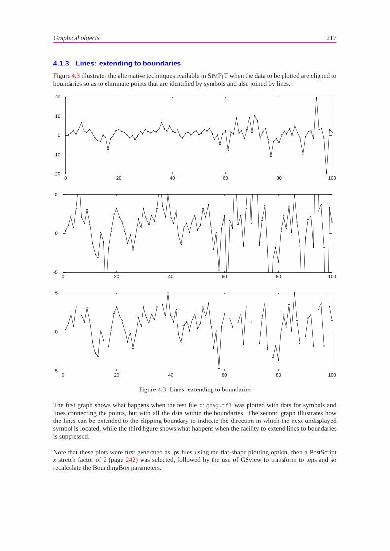
Graphical objects 217
4.1.3 Lines: extending to boundaries
Figure4.3illustrates the alternative techniques available in SIMFIT when the data to be plotted are clipped toboundaries so as to eliminate points that are identified by symbols and also joined by lines.
-20
-10
0
10
20
0 20 40 60 80 100
-5
0
5
0 20 40 60 80 100
-5
0
5
0 20 40 60 80 100
Figure 4.3: Lines: extending to boundaries
The first graph shows what happens when the test filezigzag.tf1 was plotted with dots for symbols andlines connecting the points, but with all the data within theboundaries. The second graph illustrates howthe lines can be extended to the clipping boundary to indicate the direction in which the next undisplayedsymbol is located, while the third figure shows what happens when the facility to extend lines to boundariesis suppressed.
Note that these plots were first generated as .ps files using the flat-shape plotting option, then a PostScriptx stretch factor of 2 (page242) was selected, followed by the use of GSview to transform to .eps and sorecalculate the BoundingBox parameters.

218 SIMFIT reference manual: Part 4
4.1.4 Text
Figure4.4shows how fonts can be used in any size or rotation and with many nonstandard accents, e.g.,θ.
FontsTimes-RomanTimes-ItalicTimes-BoldTimes-BoldItalicHelveticaHelvetica-ObliqueHelvetica-BoldHelvetica-BoldObliqueCourierCourier-ObliqueCourier-Bold
Courier-BoldObliqueSymbolαβχδεφγηιϕκλµνοπθρστυϖωξψζ
Size and Rotation Angle
size = 1, angle =
-90
size = 1.2, angle = -45
size = 1.4, angle = 0siz
e =
1.6,
ang
le =
45
size
= 1
.8, a
ngle
= 9
0si
ze =
2, a
ngle
= 1
10
Maths and Accents⊥ ℜ ∞ £ ℵ ⊕ ♠ ♥ ♣× ± ◊ ≈ • ÷√ ƒ ∂ ∇ ∫ ∏ ∑ → ← ↑↓ ↔ ≤ ≡ ≥ ≠ °ΑΒΓ∆ΕΖΗΘΙΚΛΜΝΞΟΠΡΣΤϒΦΧΨΩ∂∈αβγδεζηϑικλµνξοπρστυϕχψωθφ⊗ ^ ∪ ⊃ ⊂ ∃ ∋π = X = (1/n)∑X(i)T = 21°C[Ca++] = 1.2×10⁻⁹M∂φ/∂t = ∇ 2φΓ(α) = ∫tα-1e-tdt α1x + α2x
2
1 + β1x + β2x2
IsoLatin1Encoding Vector 0 1 2 3 4 5 6 7
220-227: ı ` ´ ˆ ˜ ¯ ˘ ˙230-237: ¨ ˚ ¸ ˝ ˛ ˇ240-247: ¡ ¢ £ ¤ ¥ ¦ §250-257: ¨ © ª « ¬ - ® ¯260-267: ° ± ² ³ ´ µ ¶ ·270-277: ¸ ¹ º » ¼ ½ ¾ ¿300-307: À Á Â Ã Ä Å Æ Ç
310-317: È É Ê Ë Ì Í Î Ï320-327: Ð Ñ Ò Ó Ô Õ Ö ×330-337: Ø Ù Ú Û Ü Ý Þ ß
340-347: à á â ã ä å æ ç350-357: è é ê ë ì í î ï
360-367: ð ñ ò ó ô õ ö ÷
370-377: ø ù ú û ü ý þ ÿ
Figure 4.4: Text, maths and accents.
Special effects can be created using graphics fonts such as ZapfDingbats, or user-supplied dedicated specialeffect functions, as described elsewhere (page330). Scientific symbols and simple mathematical equationscan be generated, but the best way to get complicated equations, chemical formulas, photographs or otherbitmaps into SIMFIT graphs is to use PSfrag oreditps .
Figure4.4demonstrates several possibilities for displaying mathematical formulae directly in SIMFIT graphs,and it also lists the octal codes for some commonly required characters from the IsoLatin1 encoding. Actually,octal codes can be typed in directly (e.g.,\361 instead of n), but note that text strings in SIMFIT plots canbe edited at two levels: at the simple level only standard characters can be typed in, but at the advancedlevel nonstandard symbols and maths characters can be selected from a font table. Note that, while accentscan be added individually to any standard character, they will not be placed so accurately as when using thecorresponding hard-wired characters e.g., from the IsoLatin1 encoding.

Graphical objects 219
4.1.5 Fonts, character sizes and line thicknesses
The fonts, letter sizes, and line thicknesses used in SIMFIT graphics are those chosen from the PostScriptmenu, so, whenever a font or line thickness is changed, the new details are written to the PostScript configu-ration filew_ps.cfg . If the size or thickness selected is not too extreme, it willthen be stored as the defaultto be used next time. However, it should be noted that, when the default sizes are changed, the titles, legends,labels, etc. may not be positioned correctly. You can, of course, always make a title, legend, or label fit cor-rectly by moving it about, but, if this is necessary, you may find that the defaults are restored next time youuse SIMFIT graphics. If you insist on using an extremely small or extremely large font size or line thicknessand SIMFIT keeps restoring the defaults, then you can overcome this byediting the PostScript configurationfile w_ps.cfg and making it read-only. Users who know PostScript will prefer to use the advanced PostScriptoption, whereby the users own header file can be automatically added to the PostScript file after the SIMFITdictionary has been defined, in order to re-define the fonts, line thicknesses or introduce new definitions,logos plotting symbols, etc.
4.1.6 Arrows
Figure4.5shows that arrows can be of three types: line, hollow or solidand these can be of any size. However
Arrow Types
Line Arrow
Outline Arrow
Solid Arrow
Transparent Box
Opaque Box
Arrows and Boxes
K = 1
Figure 4.5: Arrows and boxes
use can be made of headless arrows to create special effects.From this point of view a headless line arrow issimply a line which can be solid, dashed, dotted or dash-dotted. These are useful for adding arbitrary lines.A headless outline arrow is essentially a box which can be of two types: transparent or opaque. Note that theorder of priority in plotting is
Extra Text> Graphical Objects> Data plotted, titles and legends
and this allows boxes to be used to simply obliterate plotteddata or to surround extra text allowing thebackground to show through. Transparent boxes, are useful for surrounding information panels, opaqueboxes are required for chemical formulae or mathematical equations, while background colored solid boxescan be used to blank out features as shown in figure4.5. To surround a text string by a rectangular box foremphasis, position the string, generate a transparent rectangular box, then drag the opposing corners to therequired coordinates.

220 SIMFIT reference manual: Part 4
4.1.7 Polygons
Programsimplot allows filled polygons as an optional linetype. So this meansthat any set ofn coordinates(xi ,yi) can be joined up sequentially to form a polygon, which can be empty if a normal line is selected, orfilled with a chosen color if the filled polygon option is selected. If the last(xn,yn) coordinate pair is notthe same as the first(x1,y1), the polygon will be closed automatically. This technique allows the creation ofarbitrary plotting objects of any shape, as will be evident from the sawtooth plot and stars in figure4.6.
0
5
10
15
0 5 10 15 20
Plotting Polygons
x
y
Figure 4.6: Polygons
The sawtooth graph above was generated from a set of(x,y) points in the usual way, by suppressing theplotting symbol but then requesting a filled polygon linetype, colored light gray. The open star was generatedfrom coordinates that formed a closed set, but then suppressing the plotting symbol and requesting a normal,i.e. solid linetype. The filled star was created from a similar set, but selecting a filled polygon linetype,colored black.
If you create a set of ASCII text plotting coordinates files containing arbitrary polygons, such as logos orspecial plotting symbols, these can be added to any graph. However, since the files will simply be sets ofcoordinates, the position and aspect ratio of the resultingobjects plotted on your graph will be determinedby the ranges you have chosen for thex andy axes, and the aspect ratio chosen for the plot. Clearly, objectscreated in this way cannot be dragged and dropped or re-scaled interactively. The general rule is that theaxes, title, plot legends, and displayed data exist in a space that is determined by the range of data selectedfor the coordinate axes. However, extra text, symbols, arrows, information panels, etc. occupy a fixed spacethat does not depend on the magnitude of data plotted. So, selecting an interactive data transformation willalter the position of data dependent structures, but will not move any extra text, lines, or symbols.

Sizes and shapes 221
4.2 Sizes and shapes
4.2.1 Alternative axes and labels
It is useful to move axes to make plots more meaningful, and itis sometimes necessary to hide labels, as withthe plot ofy = x3 in figure4.7, where the secondx and thirdy label are suppressed. The figure also illustratesmoving an axis in barcharts with bars above and below a baseline.
-1.00
-0.50
0.50
1.00
-1.00 0.00 0.50 1.00
x
yy = x3
-5.00
-2.50
0.00
2.50
5.00
Day 0
Day 1
Day 2
Day 3
Day 4
Day 5
Day 6
Day 7
Day 8
Day 9
Time in Days
Val
ue R
ecor
ded
Figure 4.7: Axes and labels
4.2.2 Transformed data
Data should not be transformed before analysis as this distorts the error structure, but there is much to be saidfor viewing data with error bars and best fit curves in alternative spaces, and programsimplot transformsautomatically as in figure4.8.

222 SIMFIT reference manual: Part 4
0.00
1.00
2.00
0.0 10.0 20.0 30.0 40.0 50.0
Original x,y Coordinates
x
y
0.00
2.00
4.00
6.00
0.0 10.0 20.0 30.0 40.0 50.0
Dixon Plot
x
1/y
0.00
1.00
2.00
0.00 1.00 2.00 3.00 4.00 5.00
Single Reciprocal Plot
1/x
y
0.00
1.00
2.00
0.00 0.20 0.40 0.60 0.80 1.00
Eadie-Hofstee Plot
y/x
y
0.0
10.0
20.0
30.0
0.0 10.0 20.0 30.0 40.0 50.0
Hanes Plot
x
x/y
0.00
1.00
2.00
10-1 1 10 102
x-Semilog Plot
log x
y
10-2
10-1
1
10
10-1 1 10 102
Hill Plot
log x
log[
y/(A
-y)]
A = 1.8
10-1
1
10
10-1 1 10 102
Log-Log Plot
log x
log
y
2.00
4.00
6.00
-1.00 0.00 1.00 2.00 3.00 4.00 5.00
Lineweaver-Burk Plot
1/x
1/y
1:1 fit (extraploated)
2:2 fit
0.00
0.20
0.40
0.60
0.80
1.00
0.00 1.00 2.00
Scatchard Plot
y
y/x 1:1 fit (extraploated)
2:2 fit
Figure 4.8: Plotting transformed data
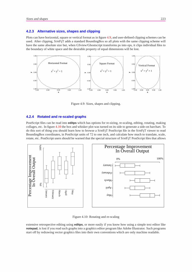
Sizes and shapes 223
4.2.3 Alternative sizes, shapes and clipping
Plots can have horizontal, square or vertical format as in figure4.9, and user-defined clipping schemes can beused. After clipping, SIMFIT adds a standard BoundingBox so all plots with the same clipping scheme willhave the same absolute size but, when GSview/Ghostscript transforms ps into eps, it clips individual files tothe boundary of white space and the desirable property of equal dimensions will be lost.
-1.00
-0.50
0.00
0.50
1.00
-1.00 -0.50 0.00 0.50 1.00
x
y
Horizontal Format
x2 + y2 = 1
-1.00
-0.50
0.00
0.50
1.00
-1.00 -0.50 0.00 0.50 1.00
x
y
Square Format
x2 + y2 = 1
-1.00
-0.50
0.00
0.50
1.00
-1.00 -0.50 0.00 0.50 1.00
x
y
Vertical Format
x2 + y2 = 1
Figure 4.9: Sizes, shapes and clipping.
4.2.4 Rotated and re-scaled graphs
PostScript files can be read intoeditps which has options for re-sizing, re-scaling, editing, rotating, makingcollages, etc. In figure4.10the box and whisker plot was turned on its side to generate a side-on barchart. Todo this sort of thing you should learn how to browse a SIMFIT PostScript file in the SIMFIT viewer to readBoundingBox coordinates, in PostScript units of 72 to one inch, and calculate how much to translate, scale,rotate, etc. PostScript users should be warned that the special structure of SIMFIT PostScript files that allows
January
February
March
April
May
Per
cent
age
Impr
ovem
ent
0%10
0%
In O
vera
ll O
utpu
t
January
February
March
April
May
Percentage Improvement
0% 100%
In Overall Output
Figure 4.10: Rotating and re-scaling
extensive retrospective editing usingeditps , or more easily if you know how using a simple text editor likenotepad , is lost if you read such graphs into a graphics editor program like Adobe Illustrator. Such programsstart off by redrawing vector graphics files into their own conventions which are only machine readable.

224 SIMFIT reference manual: Part 4
4.2.5 Changed aspect ratios and shear transformations
The barchart in figure4.11below was scaled to make the X-axis longer than the Y-axis andvice-versa, butnote how this type of differential scaling changes the aspect ratio as illustrated. Since rotation and scalingdo not commute, the effect created depends on the order of concatenation of the transformation matrices.For instance, scaling then rotation cause shearing which can be used to generate 3-dimensional perspectiveeffects as in the last sub-figure.
0.00
2.00
4.00
6.00
Bar Chart Overlaps, Groups and StacksV
alue
s
Overlap
Group
Stack
0.00
2.00
4.00
6.00
Bar Chart Overlaps, Groups and Stacks
Value
s
Overlap
GroupStack
0.00
2.00
4.00
6.00
Bar Chart Overlaps, Groups and Stacks
Va
lue
s
Overlap
Group
Stack
0.0
0
2.0
0
4.0
0
6.0
0
Bar Chart O
verlaps, G
roups and S
tack
s
Values
Overlap
Group
Stack
0.00
2.00
4.00
6.00
Bar Chart O
verla
ps, Groups a
nd Stacks
Values
Overlap
Group
Stack
Figure 4.11: Aspect ratios and shearing effects

Sizes and shapes 225
4.2.6 Reduced or enlarged graphs
Response Against Time
Res
pons
e
-5.00
-2.50
0.00
2.50
5.00
Day 0
Day 1
Day 2
Day 3
Day 4
Day 5
Day 6
Day 7
Day 8
Day 9
Response Against Time
Res
pons
e
-5.00
-2.50
0.00
2.50
5.00
Day 0
Day 1
Day 2
Day 3
Day 4
Day 5
Day 6
Day 7
Day 8
Day 9
Response Against Time
Res
pons
e
-5.00
-2.50
0.00
2.50
5.00
Day 0
Day 1
Day 2
Day 3
Day 4
Day 5
Day 6
Day 7
Day 8
Day 9
Response Against Time
Res
pons
e
-5.00
-2.50
0.00
2.50
5.00D
ay 0
Day 1
Day 2
Day 3
Day 4
Day 5
Day 6
Day 7
Day 8
Day 9
Response Against Time
Res
pons
e
-5.00
-2.50
0.00
2.50
5.00
Day 0
Day 1
Day 2
Day 3
Day 4
Day 5
Day 6
Day 7
Day 8
Day 9
Figure 4.12: Resizing fonts
It is always valuable to be able to edit a graph retrospectively, to change line or symbol types, eliminateunwanted data, suppress error bars, change the title, and soon. SIMFIT PostScript files are designed forjust this sort of thing, and a typical example would be altering line widths and font sizes as a figure isre-sized. In figure4.12 the upper sub-figures are derived from the large figure by reduction, so the textbecomes progressively more difficult to read as the figures scale down. In the lower sub-figures, however,line thicknesses and font sizes have been increased as the figure is reduced, maintaining legibility. Suchediting can be done interactively, but SIMFIT PostScript files are designed to make such retrospective editingeasy as described in thew_readme.* files and now summarized.
• Line thickness: Changing 11.00 setlinewidth to 22 setlinewidth doubles, while, e.g. 5.5 setlinewidthhalves all line thicknesses, etc. Relative thicknesses areset bysimplot .
• Fonts: Times-Roman, Times-Bold, Helvetica, Helvetica-Bold (set bysimplot ), or, in fact, any of thefonts installed on your printer.
• Texts: ti(title), xl(x legend), yl(y legend), tc(centered forx axis numbers), tl(left to right), tr(right toleft), td(rotated down), ty(centered fory axis numbers).
• Lines: pl(polyline), li(line), da(dashed line), do(dotted line), dd(dashed dotted).
• Symbols: ce(i.e. circle-empty), ch(circle-half- filled),cf(circle-filled), and similarly for triangles(te, th,tf), squares(se, sh, sf) and diamonds(de, dh, df). Coordinates and sizes are next to the abbreviations tomove, enlarge, etc.
If files do not print after editing you have probably added text to a string without padding out the key. Findthe fault using theGSview/Ghostscript package then try again.

226 SIMFIT reference manual: Part 4
4.2.7 Split axes
Sometimes split axes can show data in a more illuminating manner as in figure4.13. The options are todelete the zero time point and use a log scale to compress the sparse asymptotic section, or to cut out theuninformative part of the best fit curve between 10 and 30 days.
0.00
0.20
0.40
0.60
0.80
1.00
1.20
0 10 20 30Time (Days)
Fra
ctio
n of
Fin
al S
ize
0.00
0.20
0.40
0.60
0.80
1.00
1.20
0 2 4 6 8 10Time (Days)
Fra
ctio
n of
Fin
al S
ize
30
Figure 4.13: Split axes
Windows users can do such things with enhanced metafiles (*.emf ), but there is a particularly powerful wayfor PostScript users to split SIMFIT graphs in this way. When the SIMFIT PostScript file is being createdthere is a menu selectable shape option that allows users to chop out, re-scale, and clip arbitrary pieces ofgraphs, but in such a way that the absolute position, aspect ratio, and size of text strings does not change. Inthis way a master graph can be decomposed into any number of appropriately scaled slave sub-graphs. Theneditps can be used to compose a graph consisting of the sub-graphs rearranged, repositioned, and resized inany configuration. Figure4.13was created in this way after first adding the extra lines shown at the splittingpoint.

Sizes and shapes 227
4.2.8 Extrapolation
Best fit nonlinear curves fromqnfit can be extrapolated beyond data limits but, for purposes of illustration,extensive extrapolation of best fit models is sometimes required. For instance, fitting the mixed, or noncom-petitive inhibition model
v(S, I) =VS
K(1+ I/Kis)+ (1+ I/Kii)Sas a function of two variables is straightforward but, before the computer age, people used to fit this sort ofmodel using linear regression to the double reciprocal form
1v
=1V
(
1+I
Kii
)
+KV
(
1+I
Kis
)
which is still sometimes used to demonstrate the intersection point of the best-fit lines. Figure4.14 wasobtained by fitting the mixed model toinhibit.tf1 followed by plotting sections through the best-fit surface
-5
15
25
35
45
-5 5 10 15 20
Double Reciprocal Plot For Inhibition Data
1/S
1/v
I = 0
I = 1
I = 2
I = 3
I = 4
Figure 4.14: Extrapolation
at fixed inhibitor concentration and saving these as ASCII text files. These files (referenced by the libraryfile inhibit.tfl ) were plotted in double reciprocal space usingsimplot , and figure4.14was created byoverlaying extra lines over each best-fit line and extendingthese beyond the fixed point at
1S
= − 1K
(
Kis
Kii
)
,1v
=1V
(
1− Kis
Kii
)
.
The best-fit lines restricted to the data range were then suppressed, and the other cosmetic changes wereimplemented. It should be pointed out that, for obvious mathematical reasons, extrapolation of best fit curvesfor this model in transformed space cannot be generated by simply requesting an extended range for a best-fitcurves in the original space.

228 SIMFIT reference manual: Part 4
4.3 Equations
4.3.1 Maths
You can add equations to graphs directly but such labels willbe a compromise, since specialized type settingtechniques are required to display mathematical equationscorrectly. Now the LATEX system is pre-eminentin the field of maths type-setting and the PSfrag system, as revised by David Carlisle and others, provides asimple way to add equations to SIMFIT graphs. For figure4.15, makdat generated a Normal cdf withµ = 0andσ = 1, thensimplot createdcdf.eps with the keyphi(x) , which was then used by this stand-alone codeto generate the figure, where the equation substitutes for the key. LATEX PostScript users should be aware thatthe SIMFIT Postscript file format has been specially designed to be consistent with the PSfrag package.
\documentclass[dvips,12pt]article\usepackagegraphicx\usepackagepslatex\usepackagepsfrag\pagestyleempty
\begindocument\large\psfragphi(x)$\displaystyle
\frac1\sigma \sqrt2\pi\int_-\inftyˆx \exp\left\
-\frac12 \left( \fract-\mu\sigma \right)ˆ2 \rig ht\\,dt$\mbox\includegraphics[width=6.0in]cdf.eps\enddocument
0.50
1.00
-2.00 -1.00 0.00 1.00 2.00 3.00
x
Cumulative NormalDistribution Function
The
1
σp
2π
Z x∞exp
(12
tµ
σ
2)
dt
Figure 4.15: Plotting mathematical equations

Equations 229
4.3.2 Chemical formulæ
The technique used to combine sub-graphs into a composite graph is easy. First use your drawing or paintingprogram to save the figures of interest in the form of eps files.Then the SIMFIT graphs and any componenteps files are read intoeditps to move them and scale them until the desired effect is achieved. In figure4.16,data were generated usingdeqsol , error was added usingadderr , the simulated experimental data were fittedusingdeqsol , the plot was made usingsimplot , the chemical formulae and mathematical equations weregenerated using LATEX and the final graph was composed usingeditps .
0.00
0.20
0.40
0.60
0.80
1.00
1.20
0.00 1.00 2.00 3.00 4.00 5.00
t (min)
x(t)
, y(t
), z
(t)
x(t)
y(t)
z(t)
A kinetic study of the oxidation of p-Dimethylaminomethylbenzylamine"" bbbb ""bb""CH2NH2
CH2N(Me)2
-[O] "" bbbb ""bb""CH=0
CH2N(Me)2
+ NH3-[O] "" bbbb ""bb""C02H
CH2N(Me)2
ddt
0@ xyz
1A=0@ k+1 k1 0k+1 (k1k+2) k2
0 k+2 k2
1A0@ xyz
1A ;0@ x0
y0
z0
1A=0@ 100
1A
Figure 4.16: Chemical formulas

230 SIMFIT reference manual: Part 4
4.4 Bar charts and pie charts
4.4.1 Perspective effects
Perspective can be useful in presentation graphics but it must be realized that, when pie chart segments aremoved centrifugally, spaces adjacent to large segments open more than those adjacent to small sections. Thiscreates an impression of asymmetry to the casual observer, but it is geometrically correct. Again, diminishedcurvature compared to the perimeter as segments move out becomes more noticeable where adjacent seg-ments have greatly differing sizes so, to minimize this effect, displacements can be adjusted individually. APostScript special (page345) has been used to display the logo in figure4.17.
SIMFITSIMFITSIMFITSIMFITSIMFITSIMFITSIMFITSIMFITSIMFITSIMFITSIMFITSIMFITSIMFITSIMFITSIMFITSIMFITSIMFITSIMFITSIMFITSIMFIT
Style 1
Style 2
Style 3
Style 4
Style 5
Style 6
Style 7
Style 8
Style 9
Style 10
Pie Chart Fill Styles
Pie key 1
Pie key 2
Pie key 3
Pie key 4
Pie key 5
Pie key 6
Pie key 7
Pie key 8
Pie key 9
Pie key 10
SIMFITSIMFITSIMFITSIMFITSIMFITSIMFITSIMFITSIMFITSIMFITSIMFITSIMFITSIMFITSIMFITSIMFITSIMFITSIMFITSIMFITSIMFITSIMFITSIMFIT
-2.50
0.00
2.50
5.00
7.50
January
February
March
April
May
Perspective Effects In Bar Charts
Ran
ges,
Qua
rtile
s, M
edia
ns
Figure 4.17: Perspective in barcharts, box and whisker plots and piecharts

Pie charts and bar charts 231
4.4.2 Advanced barcharts
SIMFIT can plot barcharts directly from data matrices, using the exhaustive analysis of a matrix procedurein simstat , but there is also an advanced barchart file format which gives users complete control over everyindividual bar, etc. as now summarized and illustrated in figure4.18.
• Individual bars can have arbitrary position, width, fill style and color.
• Bars can be overlapped, grouped, formed into hanging groupsor stacked vertically.
• Error bars can be capped or straight, and above or below symbols.
• Extra features such as curves, arrows, panel identifiers or extra text can be added.
Bar Chart Features
Overlapping Group
Normal Group
Stack
Hanging Group
Box/Whisker
55%
0%
-35%
Figure 4.18: Advanced bar chart features
Of course the price that must be paid for such versatility is that the file format is rather complicated and thebest way to understand it is to consult thew_readme files for details, browse the test filesbarchart.tf? ,then read them intosimplot to observe the effect produced before trying to make your ownfiles. Labels canbe added automatically, appended to the data file, edited interactively, or input as simple text files.

232 SIMFIT reference manual: Part 4
4.4.3 Three dimensional barcharts
The SIMFIT surface plotting function can be used to plot three dimensional bars as, for example, using thetest filebarcht3d.tf1 to generate figure4.19. Blank rows and shading can also be added to enhance thethree dimensional effect.
Three Dimensional Bar Chart
JuneMay
AprilMarch
FebruaryJanuary
Year 1Year 2
Year 3Year 4
Year 5
0%
100%
50%
Three Dimensional Bar Chart
JuneMay
AprilMarch
FebruaryJanuary
Year 1
Year 2
0%
100%
50%
Figure 4.19: Three dimensional barcharts
Such plots can be created fromn by m matrix files, or special vector files, e.g. withn values forx andmvalues fory anm+6 vector is required withn, thenm, then the range ofx and range ofy, say(0,1) and(0,1)if arbitrary, followed by values off (x,y) in order of increasingx at consecutive increasing values ofy.

Error bars 233
4.5 Error bars
4.5.1 Error bars with barcharts
Barcharts can be created interactively from a table of values. For example, figure4.20was generated by theexhaustive analysis of a matrix procedure insimstat from matrix.tf1 .
0.
10.
20.
30.
Label 1
Label 2
Label 3
Label 4
Label 5
Original Axes
x
y
0
5
10
15
20
25
30
35
April May June July August
Num
ber
Infe
cted
Figure 4.20: Error bars 1: barcharts
If the elements are measurements, the bars would be means, while error bars should be calculated as 95%confidence limits, i.e. assuming a normal distribution. Often one standard error of the mean is used insteadof confidence limits to make the data look better, which is dishonest. If the elements are counts, approximateerror bars should be added to the matrix file insimplot from a separate file, using twice the square root of thecounts, i.e. assuming a Poisson distribution. After creating barcharts from matrices, the temporary advancedbarchart files can be saved.

234 SIMFIT reference manual: Part 4
4.5.2 Error bars with skyscraper and cylinder plots
Barcharts can be created for tables,z(i, j) say, where cells are values for plotting as a function ofx (rows) andy (columns). Thex,y values are not required, as such plots usually require labels not numbers. Figure4.21shows the plot generated bysimplot from the test filematrix.tf2 .
Values
Month 7Month 6
Month 5Month 4
Month 3Month 2
Month 1
Case 1Case 2
Case 3Case 4
Case 5
0
11
Simfit Skyscraper Plot with Error Bars
Values
Month 7Month 6
Month 5Month 4
Month 3Month 2
Month 1
Case 1Case 2
Case 3Case 4
Case 5
0
11
Simfit Cylinder Plot with Error Bars
Figure 4.21: Error bars 2: skyscraper and cylinder plots
Errors are added from a file, and are calculated according to the distribution assumed. They could be twicesquare roots for Poisson counts, binomial errors for proportions or percentages, or they could be calculatedfrom sample standard deviations using thet distribution for means. As skyscraper plots with errors aredominated by vertical lines, error bars are plotted with thickened lines, but a better solution is to plot cylindersinstead of skyscrapers, as illustrated.

Error bars 235
4.5.3 Slanting and multiple error bars
Error bar files can be created by programeditfl after editing curve fitting files with all replicates, and sucherror bars will be symmetrical, representing central confidence limits in the original(x,y) space. But, note thatthese error bars can become unsymmetrical or slanting as a result of a transformation, e.g. log(y) or Scatchard,using programsimplot . Programbinomial will, on the other hand, always generates noncentral confidencelimits, i.e. unsymmetrical error bars for binomial parameter confidence limits, and Log-Odds plots.
However, sometimes it is necessary to plot asymmetrical error bars, slanting error bars or even multiple errorbars. To understand this, note that the standard error bar test file errorbar.tf1 contains four columns withthex coordinate for the plotting symbol, then they-coordinates for the lower bar, middle bar and upper bar.However, the advanced error bar test fileerrorbar.tf2 has six columns, so that the(x1,y1),(x2,y2),(x3,y3)coordinates specified, can create any type of error bar, evenmultiple error bars, as will be seen in figure4.22.
0.0
2.0
4.0
6.0
0.0 2.0 4.0 6.0
Slanting and Multiple Error Bars
x
y
Figure 4.22: Error bars 3: slanting and multiple
Note that the normal error bar files created interactively from replicates byeditfl , qnfit , simplot , or comparewill only have four columns, likeerrorbar.tf1 , with x,y1,y2,y3, in that order. The six-column files likeerrorbar.tf2 required for multiple, slanting, or unsymmetrical error bars must be created as matrix fileswith the columns containingx1,x2,x3,y1,y2,y3, in that order.
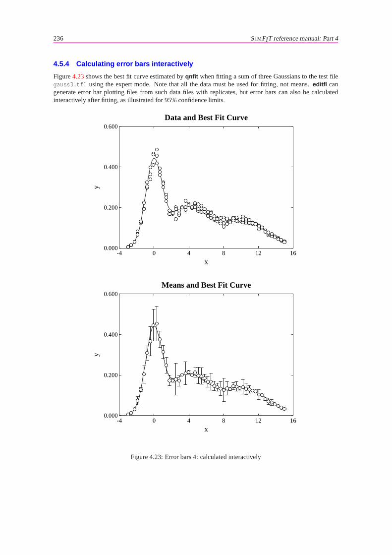
236 SIMFIT reference manual: Part 4
4.5.4 Calculating error bars interactively
Figure4.23shows the best fit curve estimated byqnfit when fitting a sum of three Gaussians to the test filegauss3.tf1 using the expert mode. Note that all the data must be used for fitting, not means.editfl cangenerate error bar plotting files from such data files with replicates, but error bars can also be calculatedinteractively after fitting, as illustrated for 95% confidence limits.
0.000
0.200
0.400
0.600
-4 0 4 8 12 16
Data and Best Fit Curve
x
y
0.000
0.200
0.400
0.600
-4 0 4 8 12 16
Means and Best Fit Curve
x
y
Figure 4.23: Error bars 4: calculated interactively

Error bars 237
4.5.5 Binomial parameter error bars
Figure4.24shows binomial parameter estimates fory successes inN trials. The error bars represent exact,unsymmetrical confidence limits (see page185), not those calculated using the normal approximation.
0.00
0.50
1.00
0 1 2 3 4 5
Binomial Parameter Estimates
Control Variable x
p =
y/N
Figure 4.24: Error bars 4: binomial parameters
4.5.6 Log-Odds error bars
Figure 4.24 can also be manipulated by transforming the estimates ˆp = y/N and confidence limits. Forinstance, the ratio of success to failure (i.e. Oddsy/(N−y)) or the logarithm (i.e. Log Odds) can be used, asin figure4.25, to emphasize deviation from a fixedp value, e.g.p = 0.5 with a log-odds of 0. Figure4.25was created from a simple log-odds plot by using the [Advanced] option to transfer thex, p/(1− p) data intosimplot , then selecting a reversey-semilog transform.
1
2
3
4
5
-1.50 -0.50 0.50 1.50
Log Odds Plot
log10[p/(1 - p)]y]
Con
trol
Var
iabl
e x
Figure 4.25: Error bars 5: log odds

238 SIMFIT reference manual: Part 4
4.5.7 Log-Odds-Ratios error bars
-1.00 -0.50 0.00 0.50 1.00 1.50
log10[Odds Ratios]
met
a.tf1
met
a.tf2
met
a.tf3
Figure 4.26: Error bars 6: log odds ratios
It is often useful to plot Log-Odds-Ratios, so thecreation of figure4.26will be outlined.
(1) The dataTest filesmeta.tf1 , meta.tf2 , andmeta.tf3 wereanalyzed in sequence using the SIMFIT Meta Anal-ysis procedure (page125). Note that, in these files,column 3 contains spacing coordinates so that datawill be plotted consecutively.
(2) The ASCII coordinate filesDuring Meta Analysis, 100(1− α)% confidencelimits on the Log-Odds-Ratio resulting from a 2 by2 contingency tables with cell frequenciesni j can beconstructed from the approximation ˆewhere
e= Zα/2
√
1n11
+1
n12+
1n21
+1
n22.
When Log-Odds-Ratios with error bars are dis-played, the overall values (shown as filled symbols)with error bars are also plotted with ax coordinateone less than smallestx value on the input file. Forthis figure, error bar coordinates were transferredinto the project archive using the [Advanced] optionto save ASCII coordinate files.
(3) Creating the composite plotProgram simplot was opened and the six errorbar coordinate files were retrieved from the projectarchive. Experienced users would do this moreeasily using a library file of course. Reversey-semilog transformation was selected, symbols werechosen, axes, title, and legends were edited, thenhalf bracket hooks identifying the data were addedas arrows and extra text.
(4) Creating the PostScript fileVertical format was chosen then, using the option tostretch PostScript files (page242), they coordinatewas stretched by a factor of two.
(5) Editing the PostScript fileTo create the final PostScript file for LATEX a tighterbounding box was calculated usinggsview then,using notepad , clipping coordinates at the top ofthe file were set equal to the BoundingBox coor-dinates, to suppress excess white space. This canalso be done using the [Style] option to omit paint-ing a white background, so that PostScript files arecreated with transparent backgrounds, i.e. no whitespace, and clipping is irrelevant.

Statistical graphs 239
4.6 Statistical graphs
4.6.1 Clusters, connections, correlations, and scattergr ams
Clusters are best plotted as sideways displaced and reducedsymbols, while connections need individual datafiles for distinct lines and symbols, as in figure4.27.
1
2
3
4
5
Plotting Clusters and ConnectionsS
core
s an
d A
vera
ges
ScoresSmithJonesBrownBell
January
February
March
AprilM
ayJune
Figure 4.27: Clusters and connections
Since the correlation coefficientr andm1,m2, the regression slopes fory(x) andx(y), are related by|r| =√m1m2, SIMFIT plots both regression lines, as in figure4.28. Other alternatives are plotting the major, or
7.00
7.50
8.00
8.50
10.0 10.5 11.0 11.5
Wing Length (cm)
Tai
l Len
gth
(cm
)
Figure 4.28: Correlations and scattergrams
reduced major axes single best fit lines, which allow for variation in bothx andy, or indicating the inclinationof the best fit bivariate normal distribution by confidence ellipses, as discussed next.

240 SIMFIT reference manual: Part 4
4.6.2 Bivariate confidence ellipses
For ap-variate normal sample of sizen with mean ¯x and variance matrix estimateS, the region
P
(x−µ)TS−1(x−µ) ≤ p(n−1)
n(n− p)Fα
p,n−p
≤ 1−α
can be regarded as a 100(1−α)% confidence region forµ. Figure4.29illustrates this for columns 1 and 2 ofcluster.tf1 discussed previously (page132). Alternatively, the region satisfying
P
(x− x)TS−1(x− x) ≤ p(n2−1)
n(n− p)Fα
p,n−p
≤ 1−α
can be interpreted as a region that with probability 1−α would contain another independent observationx,as shown for the swarm of points in figure4.29. Theµ confidence region contracts with increasingn, limitingapplication to small samples, but the new observation ellipse does not, making it useful for visualizing if datado represent a bivariate normal distribution, while inclination of the principal axes away from parallel withthe plot axes demonstrates linear correlation. This technique is only justified if the data are from a bivariatenormal distribution and are independent of the variables inthe other columns, as indicated by the correlationmatrix.
0
5
10
15
20
25
0 5 10 15 20
99% Confidence Region for the Mean
Column 1
Col
umn
2
-20
-10
0
10
20
-8 -4 0 4 8
95% Confidence Region for New Observation
x
y
Figure 4.29: Confidence ellipses for a bivariate normal distribution

Statistical graphs 241
4.6.3 Dendrograms 1: standard format
Dendrogram shape is arbitrary in two ways; thex axis order is arbitrary as clusters can be rotated around anyclustering distance leading to 2n−1 different orders, and the distance matrix depends on the settings used. Forinstance, a square root transformation, Bray-Curtis similarity, and a group average link generates the seconddendrogram in figure4.30from the first. They plotted are dissimilarities, while labels are 100− y, whichshould be remembered when changing they axis range. Users should not manipulate dendrogram parametersto create a dendrogram supporting some preconceived clustering scheme. You can set a label threshold andtranslation distance from the [X-axis] menu so that, if the number of labels exceeds the threshold, evennumbered labels are translated, and font size is decreased.
0
10
20
30
40
50
PC
1P
C6
HC
5H
C6
91A
91B
HC
7H
C8
HC
425
B61
A 5227
A10
0A 34 7630
B27
B37
B24
B26
B28
AP
C5
28B
97B
97A
PC
253
AP
C8
24A
33B 68
25A 29
32B
36B
60A
76B
61B
PC
4P
C7
PC
360
B 7331
B33
A53
B35
A37
A72
B31
A36
A32
A30
A35
B72
A99
A 4726
A99
B10
0B
Dis
tanc
e
Untransformed data
Euclidean distance
Unscaled
Single link
100%
80%
60%
40%
20%
0%
PC1PC2
PC5PC8
PC6HC8
PC3PC4
PC7HC7
HC424A
33B76B
30B100A
34
53A
76
30A
61B60A
27A27B
52
37B
68
28A
97A26A
60B29
36A36B
31B31A
35B32A
32B35A
72A72B
99A99B
37A47
100B33A
53B73
24B26B
28B97B
91A91B
25A25B
61AHC5
HC6
Per
cent
age
Sim
ilarit
y
Bray-Curtis Similarity Dendrogram
Figure 4.30: Dendrograms 1: standard format

242 SIMFIT reference manual: Part 4
4.6.4 Dendrograms 2: stretched format
100%
80%
60%
40%
20% 0%
PC1PC2PC5PC8PC6HC8PC3PC4PC7HC7HC424A33B76B30B
100A34
53A76
30A61B60A27A27B
5237B
6828A97A26A60B
2936A36B31B31A35B32A32B35A72A72B99A99B37A
47100B33A53B
7324B26B28B97B91A91B25A25B61AHC5HC6
Figure 4.31: Dendrograms 2: stretched format
SIMFIT PostScript graphs have a very useful fea-ture: you can stretch or compress the white spacebetween plotted lines and symbols without chang-ing the line thickness, symbol size, or font size andaspect ratio. For instance, stretching, clipping andsliding procedures are valuable in graphs which arecrowded due to overlapping symbols or labels, as infigure4.30. If such dendrograms are stretched ret-rospectively usingeditps , the labels will not sep-arate as the fonts will also be stretched so lettersbecome ugly due to altered aspect ratios. SIMFITcan increase white space between symbols and la-bels while maintaining correct aspect ratios for thefonts in PostScript hardcopy and, to explain this, thecreation of figure4.31will be described.
The title, legend and doublex labelling were sup-pressed, and landscape mode with stretching, clip-ping and sliding was selected from the PostScriptcontrol using the [Shape] then [Landscape +] op-tions, with anx stretching factor of two. Stretch-ing increases the space between each symbol, or thestart of each character string, arrow or other graph-ical object, but does not turn circles into ellipses ordistort letters. As graphs are often stretched to printon several sheets of paper, sub-sections of the graphcan be clipped out, then the clipped sub-sections canbe slid to the start of the original coordinate systemto facilitate printing.
If stretch factors greater than two are used, leg-ends tend to become detached from axes, and emptywhite space round the graph increases. To rem-edy the former complication, the default legendsshould be suppressed or replaced by more closelypositioned legends while, to cure the later effect,GSview can be used to calculate new BoundingBoxcoordinates (by transforming .ps to .eps). If you se-lect the option to plot an opaque background evenwhen white (by mistake), you may then find it nec-essary to edit the resulting .eps file in a text editor toadjust the clipping coordinates (identified by %#clipin the .eps file) and background polygon filling co-ordinates (identified by %#pf in the .ps file) to trimaway unwanted white background borders that areignored by GSview when calculating BoundingBoxcoordinates. Another example of this technique ison page238, where it is also pointed out that cre-ating transparent backgrounds by suppressing thepainting of a white background obviates the needto clip away extraneous white space.

Statistical graphs 243
4.6.5 Dendrograms 3: plotting subgroups
0.000.250.500.751.001.251.501.752.002.252.502.753.003.253.503.754.004.25
118
418
4050
2829
538
3611
4920
4722
2132
3712
2524
2744
246
1310
3526
3031
34
487
939
4314
236
1945
1517
3334
1642
5153
8777
7855
5966
7652
5786
6492
7974
7275
9869
8812
071
128
139
150
7384
134
124
127
147
102
143
114
122
115
101
116
137
149
104
117
138
111
148
112
105
129
133
113
140
142
146
121
144
141
145
125
109
135
5490
7081
8265
8060
5691
6268
8393
8996
9597
100
6785
6310
758
9499
6110
310
813
112
613
013
610
612
311
911
011
813
2
Dis
tanc
eFigure 4.32: Dendrograms 3: plotting subgroups
The procedure described on page242 can also beused to improve the readability of dendrogramswhere subgroups have been assigned by partial clus-tering (page140). Figure4.32shows a graph fromiris.tf1 when three subgroups are requested, or athreshold is set corresponding to the horizontal dot-ted line. Figure4.33was created by these steps.First the title was suppressed, they-axis range waschanged to(0,4.25) with 18 tick marks, the(x,y)offset was cancelled as this suppresses axis moving,the label font size was increased from 1 to 3, and thex-axis was translated to 0.8.Then the PostScript stretch/slide/clip procedure wasused with these parameters
xstretch= 1.5
ystretch= 2.0
xclip = 0.15,0.95
yclip = 0.10,0.60.
Windows users without PostScript printing facilities mustcreate a*.eps file using this technique, then usethe SIMFIT procedures to create a graphics file they can use, e.g.*.jpg . Use of a larger font and increasedx-stretching would be required to read the labels, of course.
118
418
4050
2829
538
3611
4920
4722
2132
3712
2524
2744
246
1310
3526
3031
34
487
939
4314
236
1945
1517
3334
1642
5153
8777
7855
5966
7652
5786
6492
7974
7275
9869
8812
071
128
139
150
7384
134
124
127
147
102
143
114
122
115
101
116
137
149
104
117
138
111
148
112
105
129
133
113
140
142
146
121
144
141
145
125
109
135
5490
7081
8265
8060
5691
6268
8393
8996
9597
100
6785
6310
758
9499
6110
310
813
112
613
013
610
612
311
911
011
813
2
Figure 4.33: Dendrograms 3: plotting subgroups

244 SIMFIT reference manual: Part 4
4.6.6 K-Means cluster centroids
Stretching and clipping are also valuable when graphs have to be re-sized to achieve geometrically correctaspect ratios, as in the map shown in figure4.34, which can be generated by the K-means clustering procedureusing programsimstat (see page142) as follows.
• Inputukmap.tf1 with coordinates for UK airports.
• Inputukmap.tf2 with coordinates for starting centroids.
• Calculate centroids then transfer the plot to advanced graphics.
• Read in the UK coastal outline coordinates as an extra file from ukmap.tf3 .
• Suppress axes, labels, and legends, then clip away extraneous white space.
• Stretch the PS output using the [Shape] then [Portrait +] options, and save the stretched eps file.
K-Means Clusters
Figure 4.34: K-means cluster centroids

Statistical graphs 245
4.6.7 Principal components
Principal components for multivariate data can be exploredby plotting scree diagrams and scattergramsafter using the calculations options in programsimstat . If labels are appended to the data file, as withcluster.tf2 , they can be plotted, as in figure4.35.
-0.750
-0.500
-0.250
0.000
0.250
0.500
-0.500 -0.250 0.000 0.250 0.500 0.750
PC 1
PC
2
A-1 B-2
C-3
D-4
E-5
F-6
G-7
H-8 I-9
J-10K-11
L-12
-0.750
-0.500
-0.250
0.000
0.250
0.500
-0.500 -0.250 0.000 0.250 0.500 0.750
PC 1
PC
2
A-1 B-2
C-3
D-4
F-6
G-7
H-8 I-9
K-11
E-5
J-10
L-12
Figure 4.35: Principal components
The labels that are usually plotted along thex axis are used to label the points, but moved to the side of theplotting symbol. Colors are controlled from the [Colour] options as these are linked to the color of the symbolplotted, even if the symbol is suppressed. The font is the onethat would be used to label thex axis if labelswere plotted instead of numbers. Clearly arbitrary labels cannot be plotted at the same time on thex axis.Often it is required to move the labels because of clashes, asabove. This is done by using thex axis editingfunction, setting labels that clash equal to blanks, then using the normal mechanism for adding arbitrary textand arrows to label the coordinates in the principal components scattergram. To facilitate this process, thedefault text font is the same as the axes numbering font.

246 SIMFIT reference manual: Part 4
4.6.8 Labelling statistical graphs
Labels are text strings (with associated template strings)that do not have arbitrary positions, but are plottedto identify the data. Some examples would be as follows.
• Labels adjacent to segments in a pie chart.
• Labels on theX axis to indicate groups in bar charts (page230).
• Labels on theX axis to identify clusters in dendrograms (page241).
• Labels plotted alongside symbols in 2D plots, such as principal components (page245).
Test files such ascluster.tf1 illustrate the usual way to supply labels appended to data files in order toover-ride the defaults set from the configuration options, but sometimes it is convenient to supply labelsinteractively from a file, or from the clipboard. Figure4.36 illustrates this. Test filecluster.tf1 was
0
5
10
15
20
25
0 10 20
Column 1
Col
umn
2
12
34
56
7
8
9
10
11
12
0
5
10
15
20
25
0 10 20
Column 1
Col
umn
2
Figure 4.36: Labelling statistical graphs
input into the procedure for exhaustive analysis of a matrixin simstat , and the option to plot columns asan advanced 2D plot was selected. This created the left hand figure, where default integer labels indicaterow coordinates. Then the option to add labels from a file was chosen, and test filelabels.txt was input.This is just lines of characters in alphabetical order to overwrite the default integers. Then the option to readin a template was selected, and test filetemplates.txt was input. This just contains a succession of linescontaining 6, indicating that alphabetical characters areto be plotted as bold maths symbols, resulting in theright hand figure. To summarize, the best way to manipulate labels in SIMFIT plots is as follows.
1. Write the column of case labels, or row of variable labels,from your data-base or spread-sheet programinto an ASCII text file.
2. This file should just consist of one label per line and nothing else (likelabels.txt )
3. Paste this file at the end of your SIMFIT data matrix file, editing the extra line counter (as incluster.tf1 ) as required.
4. If there aren lines of data, the extra line counter (after the data but before the labels) must be at leastn.
5. Archive the labels file if interactive use is anticipated as in figure4.36.
6. If Special symbols or accents are required, a corresponding templates file with character display codes(page341) can be prepared.

Statistical graphs 247
4.6.9 Probability distributions
Discrete probability distributions are best plotted usingvertical lines, as in figure4.37for the binomial dis-tribution but, when fitting continuous distributions, the cdf should be used since histogram shapes (and pa-rameter estimates) depend on the bins chosen. A good compromise to illustrate goodness of fit is to plot thescaledpdf along with the best fitcdf, as with the beta distribution illustrated.
0.000
0.020
0.040
0.060
0.080
0.100
0.120
0 10 20 30 40 50
Binomial Probability Plot for N = 50, p = 0.6
x
Pr(
X =
x)
0.0
10.0
20.0
0.00 0.25 0.50 0.75 1.000.00
0.20
0.40
0.60
0.80
1.00
Using QNFIT to fit Beta Function pdfs and cdfs
Random Number Values
His
togr
am a
nd p
df fi
t Step C
urve and cdf fit
Figure 4.37: Probability distributions

248 SIMFIT reference manual: Part 4
4.6.10 Survival analysis
It is often necessary to display survival data for two groupsin order to assess the relative hazards. For instance,usinggcfit in mode 3, or alternativelysimstat , to analyze the test filessurvive.tf5 andsurvive.tf6 ,which contain survival data for stage 3 (group A) and stage 4 (group B) tumors, yields the result that thesamples differ significantly according to the Mantel-Haenszel log rank test, and that the estimated value ofthe proportional hazard constant isθ = 0.3786, with confidence limits 0.1795,0.7982. Figure4.38illustratesthe Kaplan-Meier product limit survivor functions for these data using the advanced survival analysis plottingmode. In this plot, the survivor functions are extended to the end of the data range for both sets of data, even
0.00
0.25
0.50
0.75
1.00
0 50 100 150 200 250 300 350
Kaplan-Meier Product-Limit Survivor Estimates
Days from start of trial
S(t
)
Stage 3
Stage 4
+ indicates censored times
Figure 4.38: Survival analysis
though no deaths occurred at the extreme end of the time range. There are two other features of this graphthat should be indicated. The first is that the coordinates supplied for plotting were not in the form of a stairstep type of survival curve. They were just for the corners, and the step function was created by choosinga survival function step curve line type, not a cumulative probability type. Another point is that censoredobservations are also plotted, in this case using plus signsas plotting symbols, which results in the censoredobservations being identified as short vertical lines.

Statistical graphs 249
4.6.11 Goodness of fit to a Poisson distribution
After using a Kolmogorov-Smirnov 1-sample or Fisher exact test to estimate goodness of fit to a Poissondistribution, the samplecdf can be compared with the theoreticalcdf as in figure4.39. The theoreticalcdfis shown as a filled polygon for clarity. Also, sample and theoretical frequencies can be compared, as shownfor a normal graph with bars as plotting symbols, and sample values displaced to avoid overlapping. Observethat the labels atx = −1 andx = 8 were suppressed, and bars were added as graphical objects to identify thebar types.
0.0
0.2
0.4
0.6
0.8
1.0
0 1 2 3 4 5 6 7
Goodness Of Fit to a Poisson Distribution, = 3
Values
Cum
ulat
ive
Dis
trib
utio
ns
Sample (n = 25)
Theoretical cdf
0
2
4
6
8
0 1 2 3 4 5 6 7
Goodness Of Fit to a Poisson Distribution, = 3
Values
Fre
quen
cies
Theoretical
Sample (n = 25)
Figure 4.39: Goodness of fit to a Poisson distribution

250 SIMFIT reference manual: Part 4
4.6.12 Trinomial parameter joint confidence regions
A useful rule of thumb to see if parameter estimates differ significantly is to check their approximate central95% confidence regions. If the regions are disjoint it indicates that the parameters differ significantly and, infact, parameters can differ significantly even with limitedoverlap. If two or more parameters are estimated, itis valuable to inspect the joint confidence regions defined bythe estimated covariance matrix and appropriatechi-square critical value. Consider, for example, figure4.40generated by the contour plotting function ofbinomial . Data triplesx,y,z can be any partitions, such as number of male, female or dead hatchlings from abatch of eggs where it is hoped to determine a shift from equi-probable sexes. The contours are defined by
((px− px),(py− py))
[
px(1− px)/N −pxpy/N−pxpy/N py(1− py)/N
]−1(px− px
py− py
)
= χ22:0.05
whereN = x+ y+ z, px = x/N and py = y/N as discussed on page186. WhenN = 20 the triples 9,9,2and 7,11,2 cannot be distinguished, but whenN = 200 the orbits are becoming elliptical and convergingto asymptotic values. By the timeN = 600 the triples 210,330,60 and 270,270,60 can be seen to differsignificantly.
0.15
0.25
0.35
0.45
0.55
0.65
0.75
0.85
0.05 0.15 0.25 0.35 0.45 0.55 0.65 0.75
Trinomial Parameter 95% Confidence Regions
px
p y
7,11,2
70,110,20
210,330,60
9,9,290,90,20
270,270,60
Figure 4.40: Trinomial parameter joint confidence contours

Statistical graphs 251
4.6.13 Random walks
Many experimentalists record movements of bacteria or individual cells in an attempt to quantify the effectsof attractants, etc. so it is useful to compare experimentaldata with simulated data before conclusions aboutpersistence or altered motility are reached. Programrannum can generate such random walks starting fromarbitrary initial coordinates and using specified distributions. The probability density functions for the axescan be chosen independently and different techniques can beused to visualize the walk depending on thenumber of dimensions. Figure4.41shows a classical unrestricted walk on an integer grid, thatis, the stepscan be+1 with probabilityp and−1 with probabilityq = 1− p. It also shows 2- and 3-dimensional walksfor standard normal distributions.
-3
0
3
6
9
0 10 20 30 40 50
1-Dimensional Random Walk
Number of Steps
Pos
ition
-4
0
4
8
-7 -4 0 3
2-Dimensional Random Walk
x
y
3-Dimensional Random Walk
XY
Z
1
-11
11
-1-11
1
Figure 4.41: Random walks

252 SIMFIT reference manual: Part 4
4.6.14 Power as a function of sample size
It is important in the design of experiments to be able to estimate the sample size needed to detect a significanteffect. For such calculations you must specify all the parameters of interest except one, then calculate theunknown parameter using numerical techniques. For example, the problem of deciding whether one or moresamples differ significantly is a problem in the Analysis of Variance, as long as the samples are all normallydistributed and with the same variance. You specify the known variance,σ2, the minimum detectable differ-ence between means,∆, the number of groups,k, the significance level,α, and the sample size per group,n.Then, using nonlinear equations involving theF and noncentralF distributions, the power, 100(1−β) canbe calculated. It can be very confusing trying to understandthe relationship between all of these parametersso, in order to obtain an impression of how these factors alter the power, a graphical technique is very useful,as in figure4.42.
0
20
40
60
80
100
0 20 40 60 80
ANOVA (k = no. groups, n = no. per group)
Sample Size (n)
Pow
er (
%)
k =
2k
= 4
k =
8k
= 16
k =
32
2 = 1 (variance) = 1 (difference)
Figure 4.42: Power as a function of sample size
simstat was used to create this graph. The variance, significance level, minimum detectable difference andnumber of groups were fixed, then power was plotted as a function of sample size. The ASCII text coordinatefiles from several such plots were collected together into a library file to compose the joint plot usingsimplot .Note that, if a power plot reaches the current power level of interest, the critical power level is plotted (80%in the above plot) and then values either side of the intersection point are displayed.

Three dimensional plotting 253
4.7 Three dimensional plotting
4.7.1 Surfaces and contours
SIMFIT uses isometric projection, but surfaces can be viewed fromany corner, and data can be shown as asurface, contours, surface with contours, or 3-D bar chart as in figure4.43.
Using SIMPLOT to plot Probability Contours
XY
Z
1
0
1
0
0
1
Using SIMPLOT to plot a Wavy Surface
XY
Z
1
0
1
00
10
Using SIMPLOT to plot a Fluted Surface
XY
Z
1.000×10²
0.000
1.000×10²
0.0000
100
Using SIMPLOT to plot a Surface and Contours
XY
Z
1
-1
1
-1
-1
1f(x,y) = x 2 - y2
Using SIMPLOT to plot a Contour Diagram
X
Y
1.000
0.000
1.0000.000
Key Contour 1 9.025×10⁻²
2 0.181 3 0.271 4 0.361 5 0.451 6 0.542 7 0.632 8 0.722 9 0.812 10 0.903
1
1
2
2
2
2
3
3
3
4
4
4
5
5
5
6
7
89
10
Three Dimensional Bar Chart
JuneMay
AprilMarch
FebruaryJanuary
Year 1Year 2
Year 3Year 4
Year 5
0%
100%
50%
Figure 4.43: Three dimensional plotting

254 SIMFIT reference manual: Part 4
4.7.2 The objective function at solution points
SIMFIT tries to minimizeWSSQ/NDOF which has expectation unity at solution points, and it is useful toview this as a function of the parameters close to a minimum. Figure4.44shows the objective function forequation2.1after fitting 1 exponential to the test fileexfit.tf2 .
WSSQ/NDOF = f(k,A)
kA
WSSQ/NDOF
1.200
9.000×10⁻¹
1.200
9.000×10⁻¹
1
44
WSSQ/NDOF = f(Vmax,Km)
VmaxKm
WSSQ/NDOF
1.050
9.000×10⁻¹
1.150
8.500×10⁻¹
1
19
Contours for WSSQ/NDOF = f(Vmax(1),Km(1))
Vmax(1)
Km
(1)
9.800×10⁻¹
1.080
1.0609.800×10-1
Key Contour 1 1.336 2 1.581 3 1.827 4 2.073 5 2.318 6 2.564 7 2.810 8 3.055 9 3.301 10 3.546 11 3.792 12 4.038 13 4.283 14 4.529 15 4.775
1
2
2
3
3
4
4 5
5
6
6
7
7
8
8
9
9
10
10
11
11
12
12
13
131415
Figure 4.44: The objective function at solution points
The figure also shows details for equation2.4after fitting tommfit.tf2 , and for equation2.6 after fitting amodel of order 2 tommfit.tf4. Such plots are created byqnfit after fitting, by selecting any two parametersand ranges of variation. Information about the eccentricity is also available from the parameter covariancematrix, and the eigenvalues and condition number of the Hessian matrix in internal coordinates. Some contourdiagrams show long valleys at solution points, sometimes deformed considerably from ellipses, illustratingthe increased difficulty encountered with such ill-conditioned problems.

Three dimensional plotting 255
4.7.3 Sequential sections across best fit surfaces
Figure4.45shows the best fit surface after usingqnfit to fit an inhibition kinetics model. Such surfaces canalso be created for functions of two variables usingmakdat .
Inhibition Kinetics: v = f([S],[I])
[S][I]
v = f([S],[I])
8.000×101
0.000
2.000
0.000
0
89
Inhibition Kinetics: v = f([S],[I])
[S]/mM
v([S
],[I])
/M
.min
-1
0
20
40
60
80
100
0 20 40 60 80
[I] = 0
[I] = 0.5mM
[I] = 1.0mM
[I] = 2.0mM
Figure 4.45: Sequential sections across best fit surfaces
Also, qnfit allows slices to be cut through a best fit surface for fixed values of either variable. Such com-posite plots show successive sections through a best fit surface, and this is probably the best way to visualizegoodness of fit of a surface to functions of two variables.

256 SIMFIT reference manual: Part 4
4.7.4 Plotting contours for Rosenbrock optimization traje ctory
Care is sometimes needed to create satisfactory contour diagrams, and it helps both to understand the mathe-matical properties of the functionf (x,y) being plotted, and also to appreciate how SIMFIT creates a defaultcontour diagram from the function values supplied. The algorithm for creating contours first performs a scanof the function values for the minimum and maximum values, then it divides the interval into an arithmeticprogression, plots the contours, breaks the contours randomly to add keys, and prints a table of contour val-ues corresponding to the keys. As an example, consider figure4.46which plots contours for Rosenbrock’sfunction (page320)
f (x,y) = 100(y−x2)2 +(1−x)2
in the vicinity of the unique minimum at (1,1). For smooth contours, 100 divisions were used on each axis,
Contours for Rosenbrock Optimization Trajectory
X
Y
-1.500
1.500
1.500-1.500
Key Contour 1 1.425 2 2.838 3 5.663 4 11.313 5 22.613 6 45.212 7 90.412 8 1.808×10²
9 3.616×10²
10 7.232×10²
1
2
2
3
3
4
4
5
56
6
7
7
8
8
9 9
10 10
Figure 4.46: Contour diagram for Rosenbrock optimization trajectory
and user-defined proportionately increasing contour spacing was used to capture the shape of the functionaround the minimum. If the default arithmetic or geometric progressions are inadequate, as in this case, userscan select contour spacing by supplying a vector of proportions, which causes contours to be placed at thoseproportions of the interval between the minimum and maximumfunction values. The number of contourscan be varied, and the keys and table of contour values can be suppressed. The optimization trajectory andstarting and end points were supplied as extra data files, as described on page320.

Three dimensional plotting 257
4.7.5 Three dimensional space curves
Sets ofx,y,z coordinates can be plotted in three dimensional space to represent either an arbitrary scatter ofpoints, a surface, or a connected space curve. Arbitrary points are best plotted as symbols such as circles ortriangles, surfaces are usually represented as a mesh of orthogonal space curves, while single space curvescan be displayed as symbols or may be connected by lines. For instance, space curves of the form
x = x(t),y = y(t),z= z(t)
can be plotted by generatingx,y,z data for constant increments oft and joining the points together to createa smooth curve as in figure4.47.
x(t), y(t), z(t) curve and projection onto y = - 1
XY
Z
1.000
-1.000
1.000
-1.0000.000
1.000
Figure 4.47: Space curves and projections
Such space curves can be generated quite easily by preparingdata files with three columns ofx,y,z data val-ues, then displaying the data using the space curve option insimplot . However users can also generate spacecurves fromx(t),y(t),z(t) equations, using the option to plot parametric equations insimplot or usermod .The test filehelix.mod shows you how to do this for a three dimensional helixr = r(θ). Note how the rear(x,y) axes have been subdued and truncated just short of the origin, to improve the three dimensional effect.Also, projections onto planes are generated by setting the chosen variable to a constant, or by writing modelfiles to generatex,y,z data with chosen coordinates equal to the value for the plane.

258 SIMFIT reference manual: Part 4
4.7.6 Projecting space curves onto planes
Sometimes it is useful to project space curves onto planes for purposes of illustration. Figure4.48shows asimulation usingusermod with the model filetwister.mod . The parametric equations are
x = t cost,y = t sint,z= t
and projections are created by fixing one the variables to a constant value.
Twister Curve with Projections onto Planes
-20
20
-20
20
-10
0
10
-10
0
10
0
400
100
200
300
z(t)
x(t)y(t)
Figure 4.48: Projecting space curves onto planes
Note the following about the model filetwister.mod .
• There are 3 curves so there are 9 functions of 1 variable
• The value ofx supplied is used as the parametert
• Functionsf (1), f (4), f (7) are thex(t) profiles
• Functionsf (2), f (5), f (8) are they(t) profiles
• Functionsf (3), f (6), f (9) are thez(t) profiles
Also observe that the model parameters fix the values of the projection planes just outside the data range, at
p(1) = 20, p(2) = 20.

Three dimensional plotting 259
4.7.7 Three dimensional scatter diagrams
Often it is necessary to plot sets ofx,y,z coordinates in three dimensional space where the coordinates arearbitrary and are not functions of a parametert. This is the case when it is wished to illustrate scattering byusing different symbols for subsets of data that form clusters according to some distance criteria. For this typeof plotting, the sets ofx,y,z triples, say principal components, are collected togetheras sets of three columnmatrices, preferably referenced by a library file, and a default graph is first created. The usual aim would beto create a graph looking something like figure4.49.
Three Dimensional Scatter Plot
1
5
5
12
34 2
34
1
5
2
3
4
XY
Z
Type AType B
Figure 4.49: Three dimensional scatter plot
In this graph, the front axes have been removed for clarity, asubdued grid has been displayed on the verticalaxes, but not on the base and perpendiculars have been dropped from the plotting symbols to the base of theplot, in order to assist in the identification of clusters.
Note that plotting symbols, minus signs in this case, have been added to the foot of the perpendiculars toassist in visualizing the clustering. Also, note that distinct data sets, requiring individual plotting symbols,are identified by a simple rule; data values in each data file are regarded as representing the same cluster, i.e.each cluster must be in a separate file.

260 SIMFIT reference manual: Part 4
4.7.8 Two dimensional families of curves
Users may need to plot families of curves indexed by parameters. For instance, diffusion of a substance froman instantaneous plane source is described by the equation
f (x) =1
2√
πDtexp
(−x2
4Dt
)
which is, of course, a normal distribution withµ = 0 andσ2 = 2Dt, whereD is the diffusion constant andtis time, so that 2Dt is the mean square distance diffused by molecules in timet. Now it is easy to plot theconcentrationf (x) predicted by this equation as a function of distancex and timet given a diffusion constantD, by simulating the equation usingmakdat , saving the curves to a library file or project archive, then plottingthe collected curves. However, there is a much better way using programusermod which has the importantadvantage that families of curves indexed by parameters canbe plotted interactively. This is a more powerfultechnique which provides numerous advantages and convenient options when simulating systems to observethe behavior of the profiles as the indexing parameters vary.
Figure4.50shows the above equation plotted (in arbitrary units) usingthe model parameters
pi = 2Dti , for i = 1,2,3,4
to display the diffusion profiles as a function of time. The plot was created using the model filefamily2d.mod , which simply defines four identical equations corresponding to the diffusion equation butwith four different parameterspi . Programusermod was then used to read in the model, simulate it for theparameter values indicated, then plot the curves simultaneously.
0.00
0.20
0.40
0.60
0.80
1.00
1.20
1.40
1.60
-3 -2 -1 0 1 2 3
Diffusion From a Plane Source
Distance
Con
cent
ratio
n
0.25
0.5
0.75
1.0
Figure 4.50: Two dimensional families of curves

Three dimensional plotting 261
4.7.9 Three dimensional families of curves
Users may need to plot families of curves indexed by parameters in three dimensions. To show how this isdone, the diffusion equation dealt with previously (page260) is reformulated, usingy =
√2Dt, as
z(x,y) =1
y√
2πexp
−12
(
xy
)2
and is plotted in figure4.51 for the same parameter values used before, but now as sections through thesurface of a function of two variables.
Diffusion From a Plane Source
3
-3
1.25
0.00-2
-10
12
0.250.50
0.751.00
0.0
1.6
0.4
0.8
1.2
Z
XY
Figure 4.51: Three dimensional families of curves
This is, of course, a case of a family of parametric space curves projected onto the fixed values ofy. Now themodel filefamily3d.mod was used by programusermod to create this figure, using the option to plotn setsof parametric space curves, but you should observe a number of important facts about this model file beforeattempting to plot your own families of space curves.
• There are 4 curves so there are 12 functions of 1 variable
• Functionsf (1), f (4), f (7), f (10) are the parametert, i.e.x
• Functionsf (2), f (5), f (8), f (11) are they values, i.e.√
2Dt
• Functionsf (3), f (6), f (9), f (12) are thezvalues, i.e. the concentration profiles
Finally, it is clear thatn space curves require a model file that specifies 3n equations, but you should alsorealize that space curves cannot be plotted if there is insufficient variation in any of the independent variables,e.g. if ally = k, for some fixed parameterk.

262 SIMFIT reference manual: Part 4
4.8 Differential equations
4.8.1 Phase portraits of plane autonomous systems
When studying plane autonomous systems of differential equations it is useful to be able to generate phaseportraits. Consider, for instance a simplified version of the Lotka-Volterra predator prey equations given by
dy(1)
dx= y(1)(1−y(2))
dy(2)
dx= y(2)(y(1)−1)
which clearly has singular points at (0,0) and (1,1). Figure4.52was generated by simulating the systemusingdeqsol , then reading the vector field ASCII coordinate filevfield.tf1 into simplot and requestinga vector field type of plot. Usingdeqsol you can choose the equations, the range of independent variables,the number of grid points and the precision required to identify singularities. At each grid point the arrowdirection is defined by the right hand sides of the defining equations and the singular points are emphasizedby an automatic change of plotting symbol. Note that the arrows will not, in general, be on related orbits.
-1
0
1
2
-1 0 1 2
Phase Portrait for the Lotka-Volterra System
y(2)
y(1)
Figure 4.52: Phase portraits of plane autonomous systems

Differential equations 263
4.8.2 Orbits of differential equations
To obtain orbits where they(i) are parameterized by time, rather than in a time independentphase portrait asin figure4.53, trajectories have to be integrated and collected together. For instance the simple system
dy(1)
dx= y(2)
dy(2)
dx= −(y(1)(1+y(2))
was integrated bydeqsol for the initial conditions illustrated, then the orbits, collected together as ASCIIcoordinate files in the library fileorbits.tfl , were used to create the following orbit diagram using programsimplot . The way to create such orbit diagrams is to integrate the selected equations repeatedly for differentinitial conditions and then to store the required orbits, which is a facility available indeqsol . Clearly orbitsgenerated in this way can also be plotted as an overlay on a phase portrait in order to emphasize particulartrajectories. All that is required is to create a library filewith the portrait and orbits together and choose thevector field option in programsimplot . With this option, files with four columns are interpreted asarrowdiagrams while files with two columns are interpreted in the usual way as coordinates to be joined up to forma continuous curve.
-0.50
0.00
0.50
1.00
1.50
2.00
2.50
-1.25 0.00 1.25
Orbits for a System of Differential Equations
y(2)
y(1)
Figure 4.53: Orbits of differential equations

264 SIMFIT reference manual: Part 4
4.9 Specialized techniques
4.9.1 Deconvolution 1: Graphical deconvolution of complex models
Figure 4.54 shows the graphical deconvolution of the best fit curve fromqnfit into its three componentGaussianpdfsafter fitting the test filegauss3.tf1 .
0.000
0.100
0.200
0.300
0.400
0.500
-3.0 1.5 6.0 10.5 15.0
Deconvolution of 3 Gaussians
x
y
0.00
1.00
2.00
0.00 0.25 0.50 0.75 1.00 1.25 1.50 1.75
Deconvolution of Exponentials
x
y
Figure 4.54: Deconvolution 1: Graphical deconvolution of complex models
Graphical deconvolution, which displays graphs for the individual components making up a composite func-tions defined as the sum of these components, should always bedone after fitting sums of monomials,Michaelis-Mentens, High/Low affinity sites, exponentials, logistics or Gaussians, to assess the contribu-tion of the individual components to the overall fit, before accepting statistical evidence for improved fit.Many claims for three exponentials or Michaelis-Mentens would not have been made if this simple graphicaltechnique had been used.

Specialized techniques 265
4.9.2 Deconvolution 2: Fitting convolution integrals
Fitting convolution integrals (page303) involves parameter estimation inf (t), g(t), and( f ∗g)(t), where
( f ∗g)(t) =Z t
0f (u)g(t −u)du,
and such integrals occur as output functions from the response of a device to an input function. Sometimesthe input function can be controlled independently so that,from sampling the output function, parameters ofthe response function can be estimated, and frequently the functions may be normalized, e.g. the responsefunction may be modelled as a function integrating to unity as a result of a unit impulse at zero time. However,any one, two or even all three of the functions may have to be fitted. Figure4.55shows the graphical display
0.00
0.50
1.00
0 1 2 3 4 5
Fitting a Convolution Integral f*g
Time t
f(t)
, g(t
) an
d f*
g
f(t) = exp(-αt)
g(t) = β2 t exp(-βt)
f*g
Figure 4.55: Deconvolution 2: Fitting convolution integrals
following the fitting of a convolution integral usingqnfit where, to demonstrate the procedure to be followedfor maximum generality, replicates of the output function at unequally spaced time points have been assumed.The model isconvolv3.mod , and the data file isconvolv3.tfl , which just specifies replicates for the outputfunction resulting from
f (t) = exp(−αt)
g(t) = β2t exp(−βt).
Note how missing data forf (t) andg(t) are indicated by percentage symbols in the library file so, inthiscase, the modelconvolve.mod could have been fitted as a single function. However, by fitting as a functionof three variables but with data for only one function, a visual display of all components of the convolutionintegral evaluated at the best-fit parameters can be achieved.

266 SIMFIT reference manual: Part 4
4.9.3 Segmented models with cross-over points
Often segmented models are required with cross-over pointswhere the model equation swaps over at one ormore values of the independent variable. In figure4.56, for instance, data are simulated then fitted using themodelupdown.mod , showing how the three way get commandget3(.,.,.) can be used to swap over fromone model to another at a fixed critical point.
0.00
0.20
0.40
0.60
0.80
1.00
1.20
0.0 2.0 4.0 6.0 8.0 10.0 12.0
Up-Down Normal/Normal-Complement Model
x
f(x)
Cross-Over Point
0.00
0.20
0.40
0.60
0.80
1.00
1.20
0.0 2.0 4.0 6.0 8.0 10.0 12.0
Up-Down Normal/Normal-Complement Model
x
f(x)
Cross-Over Point
Figure 4.56: Models with cross over points
The model defined byupdown.mod is
f (x) = Φ((x− p1)/p2) for x≤ 6
= 1−Φ((x− p3)/p4) otherwise
whereΦ(.) is the cumulative normal distribution, and this is the relevant swap-over code.
x6subtractget3(1,1,2)f(1)
The get3(1,1,2) command pops thex− 6 off the stack and usesget(1) or get(2) depending on themagnitude ofx, since aget3(i,j,k) command simply pops the top value off the stack and then usesget(i)if this is negative,get(j) if this is zero (to machine precision), orget(k) otherwise. The cross-over pointcan also be fixed using an extra parameter that is then estimated, but this can easily lead to ill-determinedparameters and a rank deficient covariance matrix if the objective function is insensitive to small variationsin the extra parameter.

Specialized techniques 267
4.9.4 Plotting single impulse functions
Plotting single impulse functions, as in figure4.57, sometimes requires care due to the discontinuities.
0.0
10.0
20.0
-1.00 -0.50 0.00 0.50 1.00
x
f(x)
Impulse Functions
Heaviside
Kronecker
Impulse
Spike
Gauss
Figure 4.57: Plotting single impulse functions
These graphs were created using programusermod together with the model fileimpulse.mod , which definesthe five impulse functions of one variable described on page289, and usesa = p(1) > 0 to fix the location,andb = p(2) > 0 to set the pulse width where necessary.
• The Heaviside unit functionh(x−a). A pdf or survival curve stepped line type is required in order toplot the abrupt step atx = a.
• The Kronecker delta symbolδi j . Thex-coordinate data were edited interactively in programusermodin order to plot the vertical signal wheni = j as a distinct spike. After editing there was onex valueat preciselyx = a, where the function value is one, and one at a short distance either side, where thefunction values are zero.
• The square impulse function of unit area. Again a stepped line type is necessary to plot the abruptincrease and decrease of this discontinuous function, and it should be noted that, by decreasing thepulse width, the Dirac delta function can be simulated.
• The triangular spike function of unit area is straightforward to simulate and plot as long as the threex-coordinates for the corners of the triangles are present.
• The Gauss function of unit area is easy to plot.
Note that the model fileimpulse.mod uses scaling factors and additive constants so that all five functionscan be displayed in a convenient vertically stacked format.

268 SIMFIT reference manual: Part 4
4.9.5 Plotting periodic impulse functions
Plotting periodic impulse functions, as in figure4.58, sometimes requires care due to the discontinuities.
-5
0
5
10
15
20
-5 -3 0 3 5
x
f(x)
Square Wave
Rectified Triangle
Morse Dot
Saw Tooth
Rectified Sine
Half Sine
Unit Impulse
Periodic Impulse Functions
Figure 4.58: Plotting periodic impulse functions
These graphs were created using programusermod together with the model fileperiodic.mod , which de-fines the seven impulse functions of one variable described on page289, and usesa = p(1) > 0 to fix theperiod andb = p(2) > 0 to set the width where required.
• The square wave function oscillates between plus and minus one, so a pdf or survival curve steppedline type is required in order to plot the abrupt step atx = λa, for positive integerλ.
• The rectified triangular wave plots perfectly as long as thex-coordinate data are edited interactively inprogramusermod to include the integer multiples ofa.
• The Morse dot is just the positive part of the square wave, so it also requires a stepped line type.
• The sawtooth function is best plotted by editing thex-coordinate data to include a point immediatelyeither side of the multiples ofa.
• The rectified sine wave and half-wave merely require sufficient points to create a smooth curve.
• The unit impulse function requires a second parameter to define the widthb, and this is best plottedusing a stepped line type.
Note that the model fileperiodic.mod uses scaling factors and additive constants so that all seven functionscan be displayed in a convenient vertically stacked format.

Specialized techniques 269
4.9.6 Flow cytometry
csafit should be used with simulated data frommakcsa to become familiar with the concepts involved beforeanalyzing actual data, as this is a very specialized analytical procedure. Figure4.59demonstrates typical flowcytometry data fitting.
0
100
200
300
400
500
0 50 100 150 200 250
Using CSAFIT for Flow Cytometry Data Smoothing
Channel Number
Num
ber
of C
ells
Figure 4.59: Flow cytometry
4.9.7 Subsidiary figures as insets
This is easily achieved usingeditps with the individual PostScript files as shown in figure4.60.
0.00
1.00
2.00
0.00 1.00 2.00
t
f(t)
2 Exponentials
1 Exponential
-0.750
-0.250
0.250
0.00 1.00 2.00
t
log
10 f(
t)
log10f(t) against t
Figure 4.60: Subsidiary figures as insets

270 SIMFIT reference manual: Part 4
4.9.8 Nonlinear growth curves
Figure4.61illustrates the use of male and female plotting symbols to distinguish experimental data, whichare also very useful when plotting correlation data for males and females.
0
25
50
75
100
125
0 2 4 6 8 10
Time (weeks)
Per
cent
age
of A
vera
ge F
inal
Siz
e MALE
FEMALE
Using GCFIT to fit Growth Curves
Figure 4.61: Growth curves
4.9.9 Ligand binding species fractions
Species fractions (page190) are very useful when analyzing cooperative ligand bindingdata as in figure4.62.They can be generated from the best fit binding polynomial after fitting binding curves with programsffit , orby input of binding constants into programsimstat . At the same time other important analytical results likefactors of the Hessian and minimax indexHill slope Hill slope are also calculated.
0.00
0.20
0.40
0.60
0.80
1.00
0.00 1.00 2.00
Using SIMSTAT to Plot Species fractions for
x
Spe
cies
Fra
ctio
ns
Species 0Species 1Species 2Species 3Species 4
f(x) = 1 + x + 2x2 + 0.5x3 + 8x4
Figure 4.62: Ligand binding species fractions

Specialized techniques 271
4.9.10 Immunoassay and dose-response dilution curves
Antibodies are used in bioassays in concentrations known upto arbitrary multiplicative factors, and doseresponse curves are constructed by dilution technique, usually 1 in 2, 1 in 3, 1 in 10 or similar. By convention,plots are labelled in dilutions, or powers of the dilution factor and, with this technique, affinities can onlybe determined up to the unknown factor. Figure4.63was constructed usingmakfil in dilution mode withdilutions 1, 2, 4, 8, 16 and 32 to create a data file with concentrations 1/32, 1/16, 1/8, 1/4, 1/2, 1.hlfit fittedresponse as a function of concentration and a dilution curvewas plotted.
0%
50%
100%
0.00 0.20 0.40 0.60 0.80 1.00
Doubling Dilution Assay
Proportion of Maximum Concentration
Per
cent
age
of M
axim
um R
espo
nse
0%
50%
100%
1/1 1/2 1/4 1/8 1/16 1/32 1/64
Doubling Dilution Curve
Dilution FactorP
erce
ntag
e of
Max
imum
Res
pons
e
0%
50%
100%
1 2-1 2-2 2-3 2-4 2-5 2-6
Doubling Dilution Curve
Dilution Factor
Per
cent
age
of M
axim
um R
espo
nse
Figure 4.63: Immunoassay and dose-response dilution curves
The transformation is equivalent to plotting log of reciprocal concentration (in arbitrary units) but this is notusually appreciated. SIMPLOT can plot log(1/x) to bases 2, 3, 4, 5, 6, 7, 8 and 9 as well ase and ten,allowing users to plot trebling, quadrupling dilutions, etc. To emphasize this, intermediate gradations can beadded and labelling can be in powers of the base, as now shown.

272 SIMFIT reference manual: Part 4
4.9.11 r = r(θ) parametric plot 1: Eight leaved rose
Users can define their own models in parametric form for plotting or fitting. Figure4.64, for example, wasgenerated using the SIMFIT model filerose.mod from usermod to define an eight leaved rose inr = r(θ)form using the following code.
%Example: Eight leaved rose.............r = A*sin(4*theta): where theta = x, r = f(1) and A = p(1).............
%1 equation1 variable1 parameter%x4multiplysinp(1)multiplyf(1)%
-1
1
-1 1
Rhodoneae of Abbe Grandi, r = sin(4 )
x
y
Figure 4.64:r = r(θ) parametric plot 1. Eight leaved Rose

Specialized techniques 273
4.9.12 r = r(θ) parametric plot 2: Logarithmic spiral with tangent
Figure 4.65 illustrates the logarithmic spiralr(θ) = Aexp(θcotα), defined in SIMFIT model filecamalot.mod for A = 1, p(1) = α,x = θ, r = f (1) as follows.
1p(1)tandividexmultiplyexpf(1)
-5
0
5
-6 0 6
Logarithmic Spiral and Tangent
x
y
r(θ) Tangent
Figure 4.65:r = r(θ) parametric plot 2. Logarithmic Spiral with Tangent
This profile is used in camming devices such as Camalots and Friends to maintain a constant angleα betweenthe radius vector for the spiral and the tangent to the curve,defined intangent.mod as
r =Aexp(θ0cotα)[sinθ0− tan(θ0 +α)cosθ0]
sinθ− tan(θ0 +α)cosθ.
Figure4.65usedα = p(1) = 1.4,θ0 = P(2) = 6 andusermod to generate individual figures over the range0≤ θ = x≤ 10, thensimplot plotted the ASCII text coordinates simultaneously, a technique that can be usedto overlay any number of curves.

274 SIMFIT reference manual: Part 4

Appendix A
Distributions and special functions
Techniques for calling these functions from within user defined models are discussed starting on page291.
A.1 Discrete distribution functions
A discrete random variableX can have one ofn possible valuesx1,x2, . . . ,xn and has a mass functionfX ≥ 0and cumulative distribution function 0≤ FX ≤ 1 that define probability, expectation, and variance by
P(X = x j) = fX(x j), for j = 1,2, . . . ,n
= 0 otherwise
P(X ≤ x j) =j
∑i=1
fX(xi)
1 =n
∑i=1
fX(xi)
E(g(X)) =n
∑i=1
g(xi) fX(xi)
E(X) =n
∑i=1
xi f (xi)
V(X) =n
∑i=1
(xi −E(X))2 fX(xi)
= E(X2)−E(X)2.
A.1.1 Bernoulli distribution
A Bernoulli trial has only two possible outcomes,X = 1 orX = 0 with probabilitiesp andq = 1− p.
P(X = k) = pkq1−k for k = 0 ork = 1
E(X) = p
V(X) = pq
A.1.2 Binomial distribution
This models the case ofn independent Bernoulli trials with probability of success (i.e.Xi = 1) equal top andfailure (i.e.Xi = 0) equal toq = 1− p. The random binomial variableSn is defined as the sum of then values
275

276 SIMFIT reference manual: Part 5
of Xi without regard to order, i.e. the number of successes inn trials.
Sn =n
∑i=1
Xi
P(Sn = k) =
(
nk
)
pk(1− p)n−k, for k = 0,1,2, . . . ,n
E(Sn) = np
V(Sn) = np(1− p)
The run test, sign test, analysis of proportions, and many methods for analyzing experiments with only twopossible outcomes are based on the binomial distribution.
A.1.3 Multinomial distribution
Extending the binomial distribution tok possible outcomes of frequencyfi in a sample of sizen is describedby
P(X1 = f1,X2 = f2, . . . ,Xk = fk) =n!
f1! f2! · · · fk!pf1
1 pf22 · · · pfk
k
where f1 + f2 + · · ·+ fk = n
andp1 + p2+ · · ·+ pk = 1.
An example would be the trinomial distribution, which is used to analyse the outcome of incubating a clutchof eggs; they can hatch male, or female, or fail to hatch.
A.1.4 Geometric distribution
This is the distribution of the number of failures prior to the first success, where
P(X = k) = pqk
E(X) = q/p
V(X) = q/p2.
A.1.5 Negative binomial distribution
The probability ofk failures prior to therth success is the random variableSr , where
P(Sr = k) =
(
r +k−1k
)
prqk
E(Sr) = rq/p
V(Sr) = rq/p2.
A.1.6 Hypergeometric distribution
This models sampling without replacement, wheren objects are selected fromN objects, consisting ofM ≤ Nof one kind andN−M of another kind, and defines the random variableSn as
Sn = X1 +X2+ . . .Xn
whereXi = 1 for success withP(Xi = 1) = M/N, andXi = 0 for failure.
P(Sn = k) =
(
Mk
)(
N−Mn−k
)/(
Nn
)
, where
(
ab
)
= 0 whenb > a > 0
E(Sn) = nM/N
V(Sn) = npq(N−n)/(N−1)
Note that whenN ≫ n this reduces to the binomial distribution withp = M/N.

Statistical distributions supported by SIMFIT 277
A.1.7 Poisson distribution
This is the limiting form of the binomial distribution for largen and smallp but finitenp= λ > 0.
P(X = k) =λk
k!exp(−λ), for x = 0,1,2, . . . ,
E(X) = λV(X) = λ
The limiting result, for fixednp> 0, that
limn→∞
(
nk
)
pk(1− p)n−k =(np)k
k!exp(−np)
can be used to support the hypothesis that counting is a Poisson process, as in the distribution of bacteria inan sample, so that the error is of the order of the mean. The Poisson distribution also arises from Poissonprocesses, like radioactive decay, where the probability of k events which occur at a rateλ per unit time is
P(k events in(0,t)) =(λt)k
k!exp(−λt).
The Poisson distribution has the additive property that, givenn independent Poisson variablesXi with param-etersλ i , the sumY = ∑n
i=1Xi has a Poisson distribution with parameterλy = ∑ni=1λ i.
A.2 Continuous distributions
A continuous random variableX is defined over some range by a probability density functionfX ≥ 0 andcumulative distribution function 0≤ FX ≤ 1 that define probability, expectation, and variance by
FX(x) =
Z x
−∞fX(t)dt
P(A≤ x≤ B) = Fx(B)−FX(A)
=
Z B
AfX(t)dt
1 =
Z ∞
−∞fX(t)dt
E(g(X)) =
Z ∞
−∞g(t) fX(t)dt
E(X) =Z ∞
−∞t fX(t)dt
V(X) =
Z ∞
−∞(t −E(X))2 fX(t)dt.
In the context of survival analysis, the random survival timeX ≥ 0, with densityf (x), cumulative distributionfunctionF(x), survivor functionS(x), hazard functionh(x), and integrated hazard functionH(x) are definedby
S(x) = 1−F(x)
h(x) = f (x)/S(x)
H(x) =
Z x
0h(u)du
f (x) = h(x)exp−H(x).

278 SIMFIT reference manual: Part 5
A.2.1 Uniform distribution
This assumes that every value is equally likely forA≤ X ≤ B, so that
fX(x) = 1/(B−A)
E(X) = (A+B)/2
V(X) = (A+B)2/12.
A.2.2 Normal (or Gaussian) distribution
This has meanµ and varianceσ2 and, for convenience,X is often standardized toZ, so that ifX ∼ N(µ,σ2),thenZ = (x−µ)/σ∼ N(0,1).
fX(x) =1
σ√
2πexp
(
− (x−µ)2
2σ2
)
E(X) = µ
V(X) = σ2
Φ(z) = FX(z)
=1√2π
Z z
−∞exp(−t2/2)dt.
It is widely used in statistical modelling, e.g., the assumption of normally distributed dosage tolerance leadsto a probit regression model for the relationship between the probability of death and dose. There are severalimportant results concerning the normal distribution which are heavily used in hypothesis testing.
A.2.2.1 Example 1. Sums of normal variables
Givenn independent random variablesXi ∼ N(µi ,σ2i ), then the linear combinationY = ∑n
i=1aiXi is normallydistributed with parametersµy = ∑n
i=1aiµi andσ2y = ∑n
i=1a2i σ2
i .
A.2.2.2 Example 2. Convergence of a binomial to a normal dist ribution
If Sn is the sum ofn Bernoulli variables that can be 1 with probabilityp, and 0 with probability 1− p, thenSn is binomially distributed and, by the central limit theorem, it is asymptotically normal in the sense that
limn→∞
P
(
Sn−np√
np(1− p)≤ z
)
= Φ(z).
The argument that experimental error is the sum of many errors that are equally likely to be positive ornegative can be used, along with the above result, to supportthe view that experimental error is often approx-imately normally distributed.
A.2.2.3 Example 3. Distribution of a normal sample mean and v ariance
If X ∼ N(µ,σ2) and from a sample of sizen the sample mean
x =n
∑i=1
xi/n
and the sample variance
S2 =n
∑i=1
(xi − x)2/n
are calculated, then
(a) X ∼ N(µ,σ2/n);(b) nS2/σ2 ∼ χ2(n−1), E(S2) = (n−1)σ2/n, V(S2) = 2(n−1)σ4/n2; and(c) X andS2 are stochastically independent.

Statistical distributions supported by SIMFIT 279
A.2.2.4 Example 4. The central limit theorem
If independent random variablesXi have meanµ and varianceσ2 from some distribution, then the sumSn =
∑ni=1Xi , suitably normalized, is asymptotically normal, that is
limn→∞
P
(
Sn−nµσ√
n≤ z
)
= Φ(z), or
P(X1 +X2+ · · ·+Xn ≤ y) ≈ Φ(
y−nµσ√
n
)
.
Under appropriate restrictions, even the need for identical distributions can be relaxed.
A.2.3 Lognormal distribution
This is frequently used to model unimodal distributions that are skewed to the right, e.g., plasma concentra-tions which cannot be negative, that is, where the logarithmis presumed to be normally distributed so that,for X = exp(Y) whereY ∼ N(µ,σ2), then
fX(x) =1
σx√
2πexp
(
− (log(x)−µ)2
2σ2
)
E(X) = exp(µ+σ2/2)
V(X) = (exp(σ2)−1)exp(2µ+σ2).
A.2.4 Bivariate normal distribution
If variablesX andY are jointly distributed according to a bivariate normal distribution the density function is
fX,Y =1
2πσXσY
√
1−ρ2exp
(
−12
Q
)
whereQ =1
1−ρ2
(
(x−µX)2
σ2X
−2ρ(x−µX)(y−µY)
σXσY+
(y−µY)2
σ2Y
)
with σ2X > 0,σ2
Y > 0, and−1 < ρ < 1. Here the marginal density forX is normal with meanµX and varianceσ2
X , the marginal density forY is normal with meanµY and varianceσ2Y, and when the correlationρ is zero,X
andY are independent. At fixed probability levels, the quadraticform Q2 defines an ellipse in theX,Y planewhich will have axes parallel to theX,Y axes ifρ = 0, but with rotated axes otherwise.
A.2.5 Multivariate normal distribution
If a mdimensional random vectorX has aN(µ,Σ) distribution , the density is
fX(x) = (2π)−m/2|Σ|−1/2exp−12(x−µ)TΣ−1(x−µ).
Contours of equi-probability are defined byf (x) = k for somek > 0 as a hyper-ellipsoid inm dimensionalspace, and the density has the properties that any subsets ofX or linear transformations ofX are also multi-variate normal. Many techniques, e.g., MANOVA, assume thisdistribution.

280 SIMFIT reference manual: Part 5
A.2.6 t distribution
Thet distribution arises naturally as the distribution of the ratio of a normalized normal variateZ divided bythe square root of a chi-square variableχ2 divided by its degrees of freedomν.
t(ν) =Z
√
χ2(ν)/ν, or settingX = t(ν)
fX(x) =Γ((ν +1)/2)
Γ(ν/2)√
νπ
(
1+x2
ν
)−(ν+1)/2
E(X) = 0
V(X) = ν/(ν−2) for ν > 2.
The use of thet test for testing for equality of means with two normal samples X1, andX2 (page90), withsizesn1 andn2 and the same variance, uses the fact that the sample means arenormally distributed, while thesample variances are chi-square distributed, so that underH0,
Z =x1− x2
σ√
1/n1+1/n2
U =n1s2
1 +n2s22
σ2(n1 +n2−2)
T = Z/√
U
∼ t(n1 +n2−2)
T2 ∼ F(1,n1 +n2−2).
For the case of unequal variances the Welch approximation isused, where the above test statisticT anddegrees of freedomν calculated using a pooled variance estimate, are replaced by
T =x1− x2
√
s21/n1 +s2
2/n2
ν =(s2
1/n1 +s22/n2)
2
(s21/n1)2/(n1−1)+ (s2
2/n2)2/(n2−1).
The pairedt test (page92) uses the differencesdi = xi − yi between correlated variablesX andY and onlyassumes that the differences are normally distributed, so that the test statistic for the null hypothesis is
d =n
∑i=1
di/n
s2d =
n
∑i=1
(di − d)2/(n−1)
T = d/
√
s2d/n.
A.2.7 Cauchy distribution
This is the distribution of the ratio of two normal variables. For, instance, ifX1 ∼ N(0,1) andX2 ∼ N(0,1)then the ratioX = X1/X2 has a Cauchy distribution, whereE(X) andV(X) are not defined, with
fX =1
π(1+x2).
This is a better model for experimental error than the normaldistribution as the tails are larger than with anormal distribution. However, because of the large tails, the mean and variance are not defined, as with thetdistribution withν = 1 which reduces to a Cauchy distribution.

Statistical distributions supported by SIMFIT 281
A.2.8 Chi-square distribution
Theχ2 distribution withν degrees of freedom results from adding together the squaresof ν independentZvariables.
χ2(ν) =ν
∑i=1
z2i or, settingX = χ2(ν),
fX(x) =1
2ν/2Γ(ν/2)xν/2−1exp(−x/2)
E(X) = νV(X) = 2ν.
It is the distribution of the sample variance from a normal distribution, and is widely used in goodness of fittesting since, ifn frequenciesEi are expected andn frequenciesOi are observed, then
limn→∞
n
∑i=1
(Oi −Ei)2
Ei= χ2(ν).
Here the degrees of freedomν is justn−1 minus the number of extra parameters estimated from the data todefine the expected frequencies. Cochran’s theorem is another result of considerable importance in severalareas of data analysis, e.g., the analysis of variance, and this considers the situation whereZ1,Z2, . . . ,Zn areindependent standard normal variables that can be written in the form
n
∑i=1
Z2i = Q1 +Q2+ · · ·+Qk
where eachQi is a sum of squares of linear combinations of theZi . If the rank of eachQi is r i and
n = r1 + r2+ · · ·+ rk
then theQi have independent chi-square distributions, each withr i degrees of freedom.
A.2.9 F distribution
TheF distribution arises when a chi-square variable withν1 degrees of freedom (divided byν1) is divided byanother independent chi-square variable withν2 degrees of freedom (divided byν2).
F(ν1,ν2) =χ2(ν1)/ν1
χ2(ν2)/ν2or, settingX = F(ν1,ν2),
fX(x) =νν1/2
1 νν2/22 Γ((ν1 +ν2)/2)
Γ(ν1/2)Γ(ν2/2)x(ν1−2)/2(ν1x+ν2)
−(ν1+ν2)/2
E(X) = ν2/(ν2−2) for ν2 > 2.
The F distribution is used in the variance ratio tests and analysis of variance, where sums of squares arepartitioned into independent chi-square variables whose normalized ratios, as described above, are tested forequality, etc. as variance ratios.
A.2.10 Exponential distribution
This is the distribution of time to the next failure in a Poisson process. It is also known as the Laplace ornegative exponential distribution, and is defined forX ≥ 0 andλ > 0.
fX(x) = λ exp(−λx)
E(X) = 1/λ
V(X) = 1/λ2.

282 SIMFIT reference manual: Part 5
Note that, if 0≤ X ≤ 1 has a uniform distribution, thenY = (1/λ) log(X) has an exponential distribution.Also, when used as a model in survival analysis, this distribution does not allow for wear and tear, as thehazard function is just the constantλ, as follows:
S(x) = exp(−λx)
h(x) = λH(x) = λx.
A.2.11 Beta distribution
This is useful for modelling densities that are constrainedto the unit interval 0≤ x ≤ 1, as a great manyshapes can be generated by varying the parametersr > 0 ands> 0.
fX(x) =Γ(r +s)Γ(r)Γ(s)
xr−1(1−x)s−1
E(X) = r/(r +s)
V(X) = rs/((r +s+1)(r +s)2)
It is also used to model situations where a probability, e.g., the binomial parameter, is treated as a randomvariable, and it is also used in order statistics, e.g., the distribution of thekth largest ofn uniform (0,1)random numbers is beta distributed withr = k ands= n−k+1.
A.2.12 Gamma distribution
This distribution withx > 0, r > 0, andλ > 0 arises in modelling waiting times from Poisson processes.
fX(x) =λrxr−1
Γ(r)exp(−λx)
E(X) = r/λ
V(X) = r/λ2
Whenr is a positive integer it is also known as the Erlang density, i.e. the time to therth occurrence in aPoisson process with parameterλ.
A.2.13 Weibull distribution
This is used to model survival times where the survivor function S(x) and hazard rate or failure rate functionh(x) are defined as follows.
fX(x) = AB(Ax)B−1exp(−Ax)B
FX(x) = 1−exp(−Ax)B
S(x) = 1−FX(x)
h(x) = fX(x)/S(x)
= AB(Ax)B−1.
It reduces to the exponential distribution whenB = 1, but it is a much better model for survival times, dueto the flexibility in curve shapes whenB is allowed to vary, and the simple forms for the survivor and hazardfunctions. Various alternative parameterizations are used, for instance
fX(x) =
(
αβ
)(
x−γβ
)α−1
exp−(
x−γβ
)α
E(X) = γ+βΓ(
1α
+1
)
V(X) = β2
Γ(
2α
+1
)
−Γ2(
1α
+1
)
.

Statistical distributions supported by SIMFIT 283
A.2.14 Logistic distribution
This resembles the normal distribution and is widely used instatistical modelling, e.g., the assumption oflogistic dosage tolerances leads to a linear logistic regression model.
fX(x) =exp[(x−µ)/τ]
τ1−exp[(x−µ)/τ]2
FX(x) =exp[(x−µ)/τ]
1+exp[(x−µ)/τ]E(X) = µ
V(x) = π2τ2/3
A.2.15 Log logistic distribution
By analogy with the lognormal distribution, if logX has the logistic distribution, andµ = − logρ,κ = 1/τ,then the density, survivor function, and hazard functions are simpler than for the log normal distribution,namely
f (x) =κxκ−1ρκ
1+(ρx)κ2
S(x) =1
1+(ρx)κ
h(x) =κxκ−1ρκ
1+(ρx)κ .
A.3 Non-central distributions
These distributions are similar to the corresponding central distributions but they require an additional non-centrality parameter,λ. One of the main uses is in calculations of statistical poweras a function of samplesize. For instance, calculating the power for a chi-square test requires the cumulative probability function forthe non-central chi-square distribution.
A.3.1 Non-central beta distribution
The lower tail probability for parametersa andb is
P(X ≤ x) =∞
∑i=0
(λ/2) exp(−λ/2)
i!P(βa,b ≤ x),
where 0≤ x ≤ 1, a > 0, b > 0, λ ≥ 0, andP(βa,b ≤ x) is the lower tail probability for the central betadistribution.
A.3.2 Non-central chi-square distribution
The lower tail probability forν degrees of freedom is
P(X ≤ x) =∞
∑i=0
(λ/2)i exp(−λ/2)
i!P(χ2
ν+2i ≤ x),
wherex≥ 0, λ ≥ 0, andP(χ2k ≤ x) is the lower tail probability for the central chi-square distribution with k
degrees of freedom.

284 SIMFIT reference manual: Part 5
A.3.3 Non-central F distribution
The lower tail probabilityP(X ≤ x) for ν1 andν2 degrees of freedom isZ x
0
∞
∑i=0
(λ/2)i(ν1 +2i)(ν1+2i)/2νν2/22 exp(−λ/2)
i! B((ν1 +2i)/2,ν2/2)u(ν1+2i−2)/2[ν2 +(ν1 +2i)u]−(ν1+2i+ν2)/2du
wherex≥ 0, λ ≥ 0, andB(a,b) is the beta function for parametersa andb.
A.3.4 Non-central t distribution
The lower tail probability forν degrees of freedom is
P(X ≤ x) =1
Γ(ν/2)2(ν−2)/2
Z ∞
0Φ(
ux√ν−λ)
uν−1exp(−u2/2)du,
whereΦ(y) is the lower tail probability for the standard normal distribution and argumenty.
A.4 Variance stabilizing transformations
A number of transformations are in use that attempt to createnew data that is more approximately normallydistributed than the original data, or at least has more constant variance, as the two aims can not usuallyboth be achieved. If the distribution ofX is known, then the variance of any function ofX can of course becalculated. However, to a very crude first approximation, ifa random variableX is transformed byY = f (X),then the variances are related by the differential equation
V(Y) ≈(
dYdX
)2
V(X)
which yields f (.) on integration, e.g., ifV(Y) = constant is required, givenV(X).
A.4.1 Angular transformation
This arcsine transformation is sometimes used for binomialdata with parametersN and p, e.g., forX suc-cesses inN trials, when
X ∼ b(N, p)
Y = arcsin(√
X/N)
E(Y) ≃ arcsin(√
p)
V(Y) ≃ 1/(4N) (using radial measure).
However, note that the variance of the transformed data is only constant in situations where there are constantbinomial denominators.
A.4.2 Square root transformation
This is often used for counts, e.g., for Poisson variables with meanµ, when
X ∼ Poisson(µ)
Y =√
x
E(Y) ≃√µ
V(Y) ≃ 1/4.

Special functions supported by SIMFIT 285
A.4.3 Log transformation
When the variance ofX is proportional to a known powerα of E(X), then the power transformationY = Xβ
will stabilize variance forβ= 1−α/2. The angular and square root transformations are, of course, just specialcases of this, but a singular case of interest is the constantcoefficient of variation situationV(X) ∝ E(X)2
which justifies the log transform, as follows
E(X) = µ
V(X) ∝ µ2
Y = logX
V(Y) = k, a constant.
A.5 Special functions
A.5.1 Binomial coefficient
This is required in the treatment of discrete distributions. It is just the number of selections without regard toorder ofk objects out ofn.
(
nk
)
=n!
k!(n−k)!
=n(n−1)(n−2) · · ·(n−k+1)
k(k−1)(k−2) · · ·3.2.1
=
(
nn−k
)
A.5.2 Gamma and incomplete gamma functions
The gamma function is widely used in the treatment of continuous random variables and is defined as follows.
Γ(α) =
Z ∞
0tα−1exp(−t)dt
Γ(α +1) = αΓ(α).
So thatΓ(k) = (k−1)! for integerk≥ 0
andΓ(k+1/2) = (2k−1)(2k−3) · · ·5.3.1.√
π/2k.
The incomplete gamma functionP(x) and incomplete gamma function complementQ(x) given parameterαusually, as here, normalized by the complete gamma function, are also frequently required.
P(x,α) =1
Γ(α)
Z x
0tα−1exp(−t)dt
Q(x,α) =1
Γ(α)
Z ∞
xtα−1exp(−t)dt
As the gamma distribution function withG > 0, α > 0, andβ > 0 is
P(x,α,β) =1
βαΓ(α)
Z x
0Gα−1exp(−G/β)dG,
the incomplete gamma function is also the cumulative distribution function for a gamma distribution withsecond parameterβ equal to one.

286 SIMFIT reference manual: Part 5
A.5.3 Beta and incomplete beta functions
Using the gamma function, the beta function is then defined as
B(g,h) =Γ(g)Γ(h)
Γ(g+h)
and the incomplete beta function for 0≤ x≤ 1 as
R(x,g,h) =1
B(g,h)
Z x
0tg−1(1− t)h−1dt.
The incomplete beta function is also the cumulative distribution function for the beta distribution.
A.5.4 Exponential integrals
E1(x) =Z ∞
x
exp(−t)t
dt
Ei(x) = −Z ∞
−x
exp(−t)t
dt
wherex > 0, excluding the origin inEi(x).
A.5.5 Sine and cosine integrals and Euler’s gamma
Si(x) =
Z x
0
sintt
dt
Ci(x) = γ+ logx+
Z x
0
cost −1t
dt, x > 0
γ= limm→∞
1+12
+13
+14· · ·+ 1
m− logm
= .5772156649. . .
A.5.6 Fermi-Dirac integrals
f (x) =1
Γ(1+α)
Z ∞
0
tα
1+exp(t −x)dt
A.5.7 Debye functions
f (x) =nxn
Z x
0
tn
exp(t)−1dt, x > 0,n≥ 1
A.5.8 Clausen integral
f (x) = −Z x
0log(
2sint2
)
dt,0≤ x≤ π
A.5.9 Spence integral
f (x) =
Z x
0
− log|1− t|t
dt

Special functions supported by SIMFIT 287
A.5.10 Dawson integral
f (x) = exp(−x2)
Z x
0exp(t2)dt
A.5.11 Fresnel integrals
C(x) =
Z x
0cos(π
2t2)
dt
S(x) =Z x
0sin(π
2t2)
dt
A.5.12 Polygamma functions
The polygamma function is defined in terms of the gamma function Γ(x), or the Psi function (i.e. digammafunction)Ψ(x) = Γ′(x)/Γ(x)
ψ(n)(x) =dn+1
dxn+1 logΓ(x)
=dn
dxn ψ(x)
= (−1)n+1Z ∞
0
tnexp(−xt)1−exp(−t)
dt.
So the casen = 0 is the digamma function, the casen = 1 is the trigamma function, and so on.
A.5.13 Struve functions
Hν(z) =2(1
2z)ν√
πΓ(ν + 12)
Z π2
0sin(zcosθ)sin2ν θdθ
Lν(z) =2(1
2z)ν√
πΓ(ν + 12)
Z π2
0sinh(zcosθ)sin2ν θdθ
A.5.14 Kummer confluent hypergeometric functions
M(a,b,z) = 1+azb
+(a)2z2
(b)22!+ · · ·+ (a)nzn
(b)nn!+ · · ·
where(a)n = a(a+1)(a+2) . . .(a+n−1),(a)0 = 1
U(a,b,z) =π
sinπb
M(a,b,z)Γ(1+a−b)Γ(b)
−z1−bM(1+a−b,2−b,z)Γ(a)Γ(2−b)
U(a,n+1,z) =(−1)n+1
n!Γ(a−n)[M(a,n+1,z) logz
+∞
∑r=0
(a)rzr
(n+1)rr!ψ(a+ r)−ψ(1+ r)−ψ(1+n+ r) ]
+(n−1)!
Γ(a)z−nM(a−n,1−n,z)n
A.5.15 Abramovitz functions
The Abramovitz functions of ordern = 0,1,2 are defined forx≥ 0 as
f (x) =
Z ∞
0tnexp(−t2−x/t)dt

288 SIMFIT reference manual: Part 5
A.5.16 Legendre polynomials
The Legendre polynomialsPn(x) andPmn are defined in terms of the hypergeometric functionF or Rodrigue’s
formula for−1≤ x≤ 1 by
Pn(x) = F
(
−n,n+1,1,12(1−x)
)
=1
2nn!dn
dxn (x2−1)n
Pmn (x) = (−1)m(1−x2)m/2 dm
dxmPn(x).
A.5.17 Bessel, Kelvin, and Airy functions
Jν(z) = (12z)ν
∞
∑k=0
(− 14z2)k
k!Γ(ν +k+1)
Yν(z) =Jν(z)cos(νπ)−J−ν(z)
sin(νπ)
Iν(z) = (12z)ν
∞
∑k=0
(14z2)k
k!Γ(ν +k+1)
Kν(z) = 12π
I−ν(z)− Iν(z)sin(νπ)
berνx+ ibeiνx = exp(12νπi)Iν(x exp(1
4πi))
kerνx+ ikeiνx = exp(− 12νπi)Kν(x exp(1
4πi))
Ai(z) = 13
√z[I−1/3(ξ)− I1/3(ξ)], whereξ = 2
3z3/2
Ai′(z) = − 13z[I−2/3(ξ)− I2/3(ξ)]
Bi(z) =√
z/3[I−1/3(ξ)+ I1/3(ξ)]
Bi′(z) = (z/√
3)[I−2/3(ξ)+ I2/3(ξ)]
A.5.18 Elliptic integrals
RC(x,y) =12
Z ∞
0
dt√t +x(t +y)
RF(x,y,z) =12
Z ∞
0
dt√
(t +x)(t +y)(t +z)
RD(x,y,z) =32
Z ∞
0
dt√
(t +x)(t +y)(t +z)3
Rj(x,y,z,ρ) =32
Z ∞
0
dt
(t +ρ)√
(t +x)(t +y)(t +z)
u =Z φ
0
dθ√
1−msin2 θSN(u|m) = sinφCN(u|m) = cosφ
DN(u|m) =
√
1−msin2 φ

Special functions supported by SIMFIT 289
A.5.19 Single impulse functions
These discontinuous functions all generate a single impulse, but some of them require special techniques forplotting, which are described on page267.
A.5.19.1 Heaviside unit function
The Heaviside unit functionh(x−a) is defined as
h(x−a) = 0, for x < a
= 1, for x≥ a,
so it provides a useful way to construct models that switch definition at critical values of the independentvariable, in addition to acting in the usual way as a ramp function.
A.5.19.2 Kronecker delta function
The Kronecker delta functionδi j is defined as
δi j = 0, for i 6= j
= 1, for i = j,
which can be very useful when constructing models with simple logical switches.
A.5.19.3 Unit impulse function
The single square wave impulse functionf (x,a,b) of width 2b > 0 with unit area is defined as
f (x,a,b) = 0, for x < a−b, x > a+b
= 1/2b, for a−b≤ x≤ a+b,
so it can be used to model the Dirac delta function by using extremely small values forb.
A.5.19.4 Unit spike function
The triangular spike functionf (x,a,b) of width 2b > 0 with unit area is defined as
f (x,a,b) = 0, for x < a−b, x > a+b
= (x−a+b)/b2, for a−b≤ x≤ a
= (a+b−x)/b2, for a≤ x≤ a+b.
A.5.19.5 Gauss pdf
The probability density functionf (x,a,b) for the normal distribution with unit area is defined forb > 0 as
f (x,a,b) =1√2πb
exp
−12
(
x−ab
)2
,
which is very useful for modelling bell shaped impulse functions.
A.5.20 Periodic impulse functions
These generate pulses at regular intervals, and some of themrequire special techniques for plotting, as de-scribed on page268.

290 SIMFIT reference manual: Part 5
A.5.20.1 Square wave function
This has an amplitude of one and period of 2a > 0, and can be described fort ≥ 0,in terms of the Heavisideunit functionh(t) as
f1(t) = h(t)−2h(t−a)+2h(t−2a)−·· · ,so it oscillates between plus and minus one at eachx-increment of lengtha, with pulses of area plus andminusa.
A.5.20.2 Rectified triangular wave
This generates a triangular pulse of unit amplitude with period 2a > 0 and can be defined fort ≥ 0 as
f2 =1a
Z t
0f1(u)du
so it consists of a series of contiguous isosceles trianglesof areaa.
A.5.20.3 Morse dot wave function
This is essentially the upper half of the square wave. It has aperiod of 2a> 0 and can be defined fort ≥ 0 by
f3(t) =12[h(t)+ f1(t)] =
∞
∑i=0
(−1)ih(t − ia),
so it alternates between sections of zero and squares of areaa.
A.5.20.4 Sawtooth wave function
This consists of half triangles of unit amplitude and perioda > 0 and can be defined fort ≥ 0 by
f4(t) =ta−
∞
∑i=1
h(t − ia),
so it generates a sequence of right angled triangles with areaa/2
A.5.20.5 Rectified sine wave function
This is just the absolute value of the sine function with argumentat, that is
f5(t) = |sinat|,so it has unit amplitude and periodπ/a.
A.5.20.6 Rectified sine half-wave function
This is just the positive part of the sine wave
f6(t) =12[sinat+ |sinat|]
so it has period 2π/a.
A.5.20.7 Unit impulse wave function
This is a sequence of Dirac delta function pulses with unit area given by
f7(t) =∞
∑i=1
δ(i −at).
Of course, the width of the pulse has to be specified as a parameterb, so the function can be used to generatea spaced sequence of rectangular impulse with arbitrary width but unit area. Small values ofb simulate pulsesof the Dirac delta function at intervals of lengtha.

Appendix B
User defined models
B.1 Supplying models as a dynamic link library
This is still the best method to supply your own models, but itrequires programming skill. You can writein a language, such as Fortran or C, or even use assembler. Using this technique, you can specify your ownnumerical analysis library, or even reference other dynamic link libraries, as long as all the locations andaddresses are consistent with the other SIMFIT dynamic link libraries. Since the development of programusermod it is now only necessary to create new entries in the dynamic link library for convenience, or for verylarge sets of differential equations, or for models requiring special functions not supported byw models.dll .
B.2 Supplying models as ASCII text files
The method that has been developed for the SIMFIT package works extremely well, and can be used to createvery complex model equations, even though it requires no programming skill. You can use all the usualmathematical functions, including trigonometric and hyperbolic functions, as well as the gamma function, thelog-gamma function, the normal probability integral and the erfc function. The set of allowable functions willincrease asw models.dll is upgraded. The essence of the method is to supply an ASCII text file containinga set of instructions in reverse Polish, that is, postfix, or last in first out, which will be familiar to allprogrammers, since it is, after all, essentially the way that computers evaluate mathematical expressions.Using reverse Polish, any explicit model can be written as a series of sequential instructions without usingany brackets. Just think of a stack to which arguments are added and functions which operate on the top itemof the stack. Suppose the top item is the current value ofx and the operator log is added, then this will replacex by log(x) as the current item on the top of the stack. What happens is that the model file is read in, checked,and parsed just once to create a virtual instruction stack. This means that model execution is very rapid, sincethe file is only read once, but also it allows users to optimizethe stack operations by rolling, duplicating,storing, retrieving, and so on, which is very useful when developing code with repeated subexpressions, suchas occur frequently with systems of differential equation and Jacobians.
So, to supply a model this way, you must create an ASCII text file with the appropriate model or differentialequation. This is described in thew_readme.? files and can be best understood by browsing the test filessupplied, i.e.usermod1.tf? for functions of one variable,usermod2.tf? for functions of two variables,usermod3.tf? for functions of three variables andusermodd.tf? for single differential equations. Thespecial programusermod should be used to develop and test your models before trying them withmakdator qnfit . Note thatusermod checks your model file for syntax errors, but it also allows you to evaluate themodel, plot it, or even use it to find areas or zeros ofn functions inn unknowns.
Note that new syntax is being developed for this method, as described in thew_readme.* files. For instanceput andget commands considerably simplify the formulation of models with repeated sub-expressions.
291

292 SIMFIT reference manual: Part 5
Further details about the performance of this method for supplying mathematical models as ASCII text filescan be found in an article by Bardsley, W.G. and Prasad, N. in Computers and Chemistry (1997) 21, 71–82.
Examples will now be given in order to explain the format thatmust be adopted by users to define their ownmodels for simulation, fitting and plotting.
B.2.1 Example 1: a straight line
This example illustrates how the test fileusermod1.tf1 codes for a simple straight line.
%Example: user supplied function of 1 variable ... a straight line.............p(1) + p(2)*x.............
%1 equation1 variable2 parameters%p(1)p(2)xmultiplyaddf(1)%
Now exactly the same model but with comments added to explainwhat is going on. Note that in the modelfile, all text to the right of the instruction is treated as comment for the benefit of users and it is not referencedwhen the model is parsed.
% start of text defining model indicated by %Example: user supplied function of 1 variable ... a straight line.............p(1) + p(2)*x.............
% end of text, start of parameters indicated by %1 equation number of equations to define the model1 variable number of variables (or differential equation)2 parameters number of parameters in the model% end of parameters, start of model indicated by %p(1) put p(1) on the stack: stack = p(1)p(2) put p(2) on the stack: stack = p(1), p(2)x put an x on the stack: stack = p(1), p(2), xmultiply multiply top elements: stack = p(1), p(2)*xadd add the top elements: stack = p(1) + p(2)*xf(1) evaluate the model f(1) = p(1) + p(2)*x% end of the model definitions indicated by %
B.2.2 Example 2: damped simple harmonic motion
This time test fileusermod1.tf9 illustrates trigonometric and exponential functions.

User defined models 293
%Example: user supplied function of 1 variable ... damped SHM
Damped simple harmonic motion in the formf(x) = p(4)*exp[-p(3)*x]*cos[p(1)*x - p(2)]where p(i) >= 0
%1 equation1 variable4 parameters%p(1)xmultiplyp(2)subtractcosinep(3)xmultiplynegativeexponentialmultiplyp(4)multiplyf(1)%
B.2.3 Example 3: diffusion into a capillary
Test fileusermod1.tf8 codes for diffusion into a capillary and shows how to call special functions, in thiscase the error function complement with argument equal to distance divided by twice the square root of theproduct of the diffusion constant and time (i.e.p2).
%Example: user supplied function of 1 variable ... capillary diffusion
f(x) = p(1)*erfc[x/(2*sqrt(p(2))]
%1 equation1 variable2 parameters%xp(2)squareroot2multiplydivideerfcp(1)multiplyf(1)%

294 SIMFIT reference manual: Part 5
B.2.4 Example 4: defining three models at the same time
The test fileline3.mod illustrates the technique for defining several models for simultaneous fitting byprogramqnfit , in this case three straight lines unlinked for simplicity,although the models can be of arbitrarycomplexity and they can be linked by common parameters.
%f(1) = p(1) + p(2)x: (line 1)f(2) = p(3) + p(4)x: (line 2)f(3) = p(5) + p(6)x: (line 3)Example: user supplied function of 1 variable ... 3 straight lines
%3 equations1 variable6 parameters%p(1)p(2)xmultiplyaddf(1)p(3)p(4)xmultiplyaddf(2)p(5)p(6)xmultiplyaddf(3)%
B.2.5 Example 5: Lotka-Volterra predator-prey differenti al equations
A special extended version of this format is needed with systems of differential equations, where the associ-ated Jacobian can be supplied, as well as the differential equations if the equations are stiff and Gear’s methodis required. However, supplying the wrong Jacobian is a common source of error in differential equation solv-ing, so you should always compare results with the option to calculate the Jacobian numerically, especially ifslow convergence is suspected. A dummy Jacobian can be supplied if Gear’s method is not to be used or ifthe Jacobian is to be estimated numerically. You can even prepare a differential equation file with no Jacobianat all.
So, to develop a model file for a system of differential equations, you first of all write the model ending withtwo lines, each containing only a %. When this runs properly you can start to add code for the Jacobian byadding new lines between the two % lines. This will be clear from inspecting the large number of modelfiles provided and thereadme.* files. If at any stage the code with Jacobian runs more slowly than the codewithout the Jacobian, then the Jacobian must be coded incorrectly.
The next example is the text for test filedeqmod2.tf2 which codes for the Lotka-Volterra predator-preyequations. This time all the comments are left in and a Jacobian is coded. This can be left out entirelyby following the model by a percentage sign on two consecutive lines. SIMFIT can use the Adam’s method

User defined models 295
but can still use Gears method by estimating the Jacobian by finite differences. Note that the Jacobian isinitialized to the identity, so when supplying a Jacobian only the elements not equal to identity elements needbe set.
%Example of a user supplied pair of differential equationsfile: deqmod2.tf2 (typical parameter file deqpar2.tf2)model: Lotka-Volterra predator-prey equations
differential equations: f(1) = dy(1)/dx= p(1)*y(1) - p(2)*y(1)*y(2)
f(2) = dy(2)/dx= -p(3)*y(2) + p(4)*y(1)*y(2)
jacobian: j(1) = df(1)/dy(1)= p(1) - p(2)*y(2)
j(2) = df(2)/dy(1)= p(4)*y(2)
j(3) = df(1)/dy(2)= -p(2)*y(1)
j(4) = df(2)/dy(2)= -p(3) + p(4)*y(1)
initial condition: y0(1) = p(5), y0(2) = p(6)
Note: the last parameters must be y0(i) in differential equa tions%2 equations no. equationsdifferential equation no. variables (or differential equa tion)6 parameters no. of parameters in this model%y(1) stack = y(1)y(2) stack = y(1), y(2)multiply stack = y(1)*y(2)duplicate stack = y(1)*y(2), y(1)*y(2)p(2) stack = y(1)*y(2), y(1)*y(2), p(2)multiply stack = y(1)*y(2), p(2)*y(1)*y(2)negative stack = y(1)*y(2), -p(2)*y(1)*y(2)p(1) stack = y(1)*y(2), -p(2)*y(1)*y(2), p(1)y(1) stack = y(1)*y(2), -p(2)*y(1)*y(2), p(1), y(1)multiply stack = y(1)*y(2), -p(2)*y(1)*y(2), p(1)*y(1)add stack = y(1)*y(2), p(1)*y(1) - p(2)*y(1)*y(2)f(1) evaluate dy(1)/dxp(4) stack = y(1)*y(2), p(4)multiply stack = p(4)*y(1)*y(2)p(3) stack = p(4)*y(1)*y(2), p(3)y(2) stack = p(4)*y(1)*y(2), p(3), y(2)multiply stack = p(4)*y(1)*y(2), p(3)*y(2)subtract stack = -p(3)*y(2) + p(4)*y(1)*y(2)f(2) evaluate dy(2)/dx% end of model, start of Jacobianp(1) stack = p(1)p(2) stack = p(1), p(2)y(2) stack = p(1), p(2), y(2)

296 SIMFIT reference manual: Part 5
multiply stack = p(1), p(2)*y(2)subtract stack = p(1) - p(2)*y(2)j(1) evaluate J(1,1)p(4)y(2)multiplyj(2) evaluate J(2,1)p(2)y(1)multiplynegativej(3) evaluate J(1,2)p(4)y(1)multiplyp(3)subtractj(4) evaluate J(2,2)%
B.2.6 Example 6: supplying initial conditions
The test filedeqpar2.tf2 illustrates how initial conditions, starting estimates and limits are supplied.
Title line...(1) Parameter file for deqmod2.tf2 .. this lin e is ignored0 (2) IRELAB: mixed(0), decimal places(1), sig. digits(2)6 (3) M = number of parameters (include p(M-N+1)=y0(1), etc. )1 (4) METHOD: Gear(1), Runge_Kutta(2), Adams(3)1 (5) MPED: Jacobian estimated(0), calculated(1)2 (6) N = number of equations41 (7) NPTS = number of time points0.0,1.0,3.0 (7+1) pl(1),p(1),ph(1) parameter 10.0,1.0,3.0 (7+2) pl(2),p(2),ph(2) parameter 20.0,1.0,3.0 (7+3) pl(3),p(3),ph(3) parameter 30.0,1.0,3.0 (7+4) pl(4),p(4),ph(4) parameter 40.0,1.0,3.0 (7+5) pl(5),p(5),ph(5) y0(1)0.0,0.5,3.0 (7+M) pl(6),p(6),ph(6) y0(2)1.0e-4 (7+M+1) TOL: tolerance10.0 (7+M+2) XEND: end of integration0.0 (7+M+3) XSTART: start of integration
An initial conditions file supplies all the values required for a simulation or curve fitting problem with dif-ferential equations using programsdeqsol or qnfit . Note that the values must be supplied in exactly theabove order. The first line (title) and trailing lines after (7+M+3) are ignored. Field width for most values is12 columns, but is 36 for parameters. Comments can be added after the last significant column if required.Parameters are in the order ofpl(i) ≤ p(i) ≤ ph(i) wherepl(i) are the bottom limits,p(i) are the startingparameters andph(i) are the upper limits for curve fitting. To fix a parameter during curve fitting just setpl(i) = p(i) = ph(i). Note thatpl(i) andph(i) are used in curve fitting but not simulation. Parameters 1 toM−N are the parameters in the equations, but parametersM−N+1 to M are the initial conditions, namelyy0(1) to y0(N).
B.2.7 Example 7: transforming differential equations
If you just want information on a sub-set of the components,y(i), you can select any required components(interactively) indeqsol . If you only want to fit a sub-set of components, this is done byadding escape

User defined models 297
sequences to the input data library file as shown by the % characters in the example filesdeqsol.tf2 anddeqsol.tf3. A more complicated process is required if you are interestedonly in some linear combinationof they(i), and do not want to (or can not) re-write the differential equations into an appropriate form, evenusing conservation equations to eliminate variables. To solve this problem you can input a matrixA, thensimply choosey(new) = A∗ y(old), where after integrationy(new) replacesy(old).
Format for A-type files
The procedure is that when transformation is selected, deqsol sets A equal to the identity matrix then it readsin your file with the sub-matrix to overwriteA. TheA-file simply contains a column ofi-values,a column ofj-values and a column of correspondingA(i, j) values. To prepare such a file you can use makmat or a texteditor. Consult the test files (deqmat.tf? ) for examples.
ExamplesAn A matrix to interchangey(1) andy(2).
(
0 11 0
)
An A matrix to replacey(2) by y(1)+y(2).
1 0 00 1 10 0 1
An A matrix to replacey(2) by 0.5y(1)+2.0y(2)−y(3) then swapy(1) andy(3).
0.0 0.0 1.00.5 2.0 −1.01.0 0.0 0.0
Note the following facts.
1. You only need to supply elementsA(i, j) which differ from those of the corresponding identity matrix.
2. The program solves for the actualy(i) then makes new vectorsz(i) wherey(i) are to be transformed.Thez(i) are then copied onto the newy(i).
3. This is very important.To solve they(i) the program has to start with the actual initial conditionsy0(i).So, even if they(i) are transformed by anA which is not the identity, they0 are never transformed. Whensimulating you must remember thaty0(i) you set are truey0(i) and when curve-fitting, parametersestimated are the actualy0(i), not transformed ones.
B.2.8 Formatting conventions for user defined models
Please observe the use of the special symbol % in model files. The symbol % starting a line is an escape se-quence to indicate a change in the meaning of the input stream, e.g., from text to parameters, from parametersto model instructions, from model to Jacobian, etc. Characters occurring to the right of the first non-blankcharacter are interpreted as comments and text here is ignored when the model is parsed. The % symbolmustbe used to indicate:-
i) start of the fileii) start of the model parametersiii) start of the model equationsiv) end of model equations (start of Jacobian with diff. eqns.)
The file you supply must haveexactlythe format now described.

298 SIMFIT reference manual: Part 5
a) The file must start with a % symbol indicating where text starts The next lines must be the name/detailsyou choose for the model. This would normally be at least 4 andnot greater than 24 lines. This textis only to identify the model and is not used by SIMFIT. The end of this section is marked by a %symbol. The next three lines define the type of model.
b) The first of these lines must indicate the number of equationsin the model, e.g., 1 equation, 2 equations,3 equations, etc.
c) The next must indicate the number of independent variables as in:- 1 variable, 2 variables, 3 variables, etc.or else it could be differential equation to indicate that the model is one or a set of ordinary differentialequations with one independent variable.
d) The next line must define the number of parameters in the model.
e) With differential equations, the last parameters are reserved to set the values for the integration constantsy0(i), which can be either estimated or fixed as required. For example, if there aren equations andm parameters are declared in the file, onlym− n can be actually used in the model, sincey0(i) =p(m−n+ i) for i = 1,2, ...,n.
f) Lines are broken up into tokens by spaces.
g) Only the first token in each line matters after the model starts.
h) Comments begin with % and are added just to explain what’s going on.
i) Usually the comments beginning with a % can be omitted.
j) Critical lines starting with % must be present as explained above.
k) The model operations then follow, one per line until the nextline starting with a % character indicates theend of the model.
l) Numbers can be in any format, e.g., 2, 1.234, 1.234E-6, 1.234E6
m) The symbol f(i) indicates that model equation i is evaluatedat this point.
n) Differential equations can define the Jacobian after defining the model. If there aren differential equationsof the form
dydx
= f (i)(x,y(1),y(2), ...,y(n))
then the symboly(i) is used to puty(i) on the stack and there must be an by n matrix defined inthe following way. The elementJ(a,b) is indicated by puttingj(n(b− 1) + a) on the stack. Thatis the columns are filled up first. For instance with 3 equations you would have a JacobianJ(i, j) =d f(i)/dy( j) defined by the sequence:
J(1,1) = j(1), J(1,2) = j(4), J(3,1) = j(7)J(2,1) = j(2), J(2,2) = j(5), J(3,2) = j(8)J(3,1) = j(3), J(3,2) = j(6), J(3,3) = j(9)
B.2.8.1 Table of user-defined model commands
Command Effects produced
x stack -> stack, xy stack -> stack, yz stack -> stack, zadd stack, a, b -> stack, (a + b)subtract stack, a, b -> stack, (a - b)multiply stack, a, b -> stack, (a*b)

User defined models 299
divide stack, a, b -> stack, (a/b)p(i) stack -> stack, p(i) ... i can be 1, 2, 3, etcf(i) stack, a -> stack ...evaluate model since now f(i) = apower stack, a, b -> stack, (aˆb)squareroot stack, a -> stack, sqrt(a)exponential stack, a -> stack, exp(a)tentothepower stack, a -> stack, 10ˆaln (or log) stack, a -> stack, ln(a)log10 stack, a -> stack, log(a) (to base ten)pi stack -> stack, 3.1415927sine stack, a -> stack, sin(a) ... radians not degreescosine stack, a -> stack, cos(a) ... radians not degreestangent stack, a -> stack, tan(a) ... radians not degreesarcsine stack, a -> stack, arcsin(a) ... radians not degreesarccosine stack, a -> stack, arccos(a) ... radians not degre esarctangent stack, a -> stack, arctan(a) ... radians not degr eessinh stack, a -> stack, sinh(a)cosh stack, a -> stack, cosh(a)tanh stack, a -> stack, tanh(a)exchange stack, a, b -> stack, b, aduplicate stack, a -> stack, a, apop stack, a, b -> stack, aabsolutevalue stack, a -> stack, abs(a)negative stack, a -> stack , -aminimum stack, a, b -> stack, min(a,b)maximum stack, a, b -> stack, max(a,b)gammafunction stack, a -> stack, gamma(a)lgamma stack, a -> stack, ln(gamma(a))normalcdf stack, a -> stack, phi(a) integral from -infinity to aerfc stack, a -> stack, erfc(a)y(i) stack -> stack, y(i) Only diff. eqns.j(i) stack, a -> stack J(i-(i/n), (i/n)+1) Only diff. eqns.*** stack -> stack, *** ... *** can be any number
B.2.8.2 Table of synonyms for user-defined model commands
The following sets of commands are equivalent:-
sub, minus, subtractmul, multiplydiv, dividesqrt, squarero, squarerootexp, exponent, exponentialten, tentothe, tentothepowerln, logsin, sinecos, cosinetan, tangentasin, arcsin, arcsineacos, arccos, arccosineatan, arctan, arctangentdup, duplicateexch, exchange, swapdel, delete, popabs, absolute

300 SIMFIT reference manual: Part 5
neg, negativemin, minimummax, maximumphi, normal, normalcd, normalcdfabserr, epsabsrelerr, epsrelmiddle, mid
B.2.8.3 Error handling in user defined models
As the stack is evaluated, action is taken to avoid underflow,overflow and forbidden operations, like 1/x asx tends to zero or taking the log or square root of a negative number etc. This should never be necessary, asusers should be able to design the fitting or simulation procedures in such a way that such singularities arenot encountered, rather than relying on default actions which can lead to very misleading results.
B.2.8.4 Notation for functions of more than three variables
The model for nine equations in nine unknowns coded inusermodn.tf4 is provided to show you how to useusermod to find a zero vector for a system of nonlinear equations. It illustrates how to code for n functionsof m variables, and shows how to usey(1),y(2), . . . ,y(m) instead ofx,y,z, etc. The idea is that, when thereare more than three variables, you should not usex,y or z in the model file, you should usey(1),y(2) andy(3), etc.
B.2.8.5 The commands put(.) and get(.)
These facilitate writing complicated models that re-use previously calculated expressions (very common withdifferential equations).The commands are as follows
put(i) : move the top stack element into storage location iget(j) : transfer storage element j onto the top of the stack
and the following code gives an example.
xput(11)get(11)get(11)multiplyput(23)get(11)get(23)add : now (x + xˆ2) has been added to the top of the stack
It should be observed that these two commands reference a global store. This is particularly important when amain model calls sub-models for evaluation, root finding or quadrature, as it provides a way to communicateinformation between the models.
B.2.8.6 The command get3(.,.,.)
Often a three way branch is required where the next step in a calculation depends on whether a criticalexpression is negative, zero or positive, e.g., the nature of the roots of a quadratic equation depend on the valueof the discriminant. The way this is effected is to define the three possible actions and store the results usingthreeput commands. Then use aget3(i,j,k) command to pop the top stack element and invokeget(i)if the element is negative,get(j) if it is zero (to machine precision), orget(k) otherwise. For example, themodelupdown.mod , illustrated on page266, is a simple example of how to use aget3(.,.,.) command to

User defined models 301
define a model which swaps over from one equation to another ata critical value of the independent variable.This command can be used after the commandorder has been used to place a−1,0 or 1 on the stack, andthe modelupdownup.mod illustrates how to useorder with value3 to create a model with two swap-overpoints.
xnegativeput(5)1.0e-100put(6)xput(7)xget3(5,6,7) : now the top stack element is |x|, or 1.0e-100
B.2.8.7 The commands epsabs and epsrel
When the evaluation of a model requires iterative procedures, like root finding or quadrature, the absoluteand relative error tolerances must be specified. Default values (1.0e-6 and 1.0e-3) are initialized and theseshould suffice for most purposes. However you may need to specify alternative values by using theepasabsor epsrel commands with difficult problems, or to control the accuracyused in a calculation. For instance,when fitting a model that involves the evaluation of a multiple integral as a sub-model, you would normallyuse fairly large values for the error tolerances until a goodfit has been found, then decrease the tolerances fora final refinement. Values added to the stack to define the tolerances are popped.
1.0e-4epsabs1.0e-2epsrel : now epsabs = 0.0001 and epsrel = 0.01
B.2.8.8 The commands blim(.) and tlim(.)
When finding roots of equations it is necessary to specify starting limits and when integrating by quadratureit is necessary to supply lower and upper limits of integration. The commandblim(i) sets the lower limitfor variablei while the commandtlim(j) sets the upper limit for variablej. Values added to the stack todefine the limits are popped.
0blim(1)0blim(2)pitlim(1)pi2multiplytlim(2) :limits are now 0 < x < 3.14159 and 0 < y < 6.28318
B.2.9 Plotting user defined models
Once a model has been checked by programusermod it can be plotted directly if it is a function of one vari-able, a function of two variables, a parametric curve inr(θ) format (page272), x(t),y(t) format (page260), ora space curve inx(t),y(t),z(t) format (page261). This is also be a very convenient way to simulate familiesof curves described as separate functions of one variable, as will be readily appreciated by reading in the testfile usermodn.tf1 , which defines four trigonometric functions of one variable.

302 SIMFIT reference manual: Part 5
B.2.10 Finding zeros of user defined models
After a model function of one variable has been checked by programusermod it is possible to locate zerosof the equation
f (x)−k = 0
for fixed values ofk. It is no use expecting this root finding to work unless you know the approximate locationof a root and can supply two valuesA,B that bracket the root required, in the sense that
f (A) f (B) < 0.
For this reason, it is usual to simulate the model first and observe the plot until two sensible limitsA,B arelocated. Tryusermod.tf1 which is just a straight line to get the idea. Note that in difficult cases, whereIFAIL is not returned as zero, it will be necessary to adjust EPSABS and EPSREL, the absolute and relativeerror tolerances.
B.2.11 Finding zeros of n functions in n variables
When a model file definingn functions ofn unknowns has been checked by programusermod it is possibleto attempt to find an-vector solution givenn starting estimates, ifn > 1. As the location of such vectors usesiterative techniques, it is only likely to succeed if sensible starting estimates are provided. As an example,try the model fileusermodn.tf4 which defines nine equations in nine unknowns. Note that to obtain IFAILequal to zero, i.e. a satisfactory solution, you will have toexperiment with starting estimates. Observe thatthese are supplied using theusermod y vector, not the parameter vectorp. Try setting the nine elements ofthey vector to zero, which is easily done from a menu.
B.2.12 Integrating 1 function of 1 variable
After using programusermod to check a function of one variable, definite integration over fixed limits can bedone by two methods. Simpson’s rule is used, because users may wish to embed a straightforward Simpson’srule calculation in a model, but also adaptive quadrature isused, in case the integral is ill conditioned, e.g., hasspikes or poles. Again preliminary plotting is recommendedfor ill-conditioned functions. Tryusermod1.tf1to see how it all works.
B.2.13 Integrating n functions of m variables
When a model definingn functions ofm variables has been successfully parsed by programusermod , adap-tive integration can be attempted ifm> 1. For this to succeed, the user must set them lower limits (blim)and themupper limits (tlim) to sensible values, and it probably willbe necessary to alter the error tolerancesfor success (i.e. zero IFAIL). Where users wish to embed the calculation of an adaptive quadrature procedureinside a main model, it is essential to investigate the quadrature independently, especially if the quadrature ispart of a sub-model involving root finding. Tryusermod4.tf1 which is a single four dimensional integral(i.e. n = 1 andm= 4) that should be integrated between zero and one for all fourvariables. Observe, in thismodel, thaty(1),y(2),y(3),y(4) are the variables, becausem> 3.
B.2.14 Calling sub-models from user-defined models
B.2.14.1 The command putpar
This command is used to communicate parametersp(i) to a sub-model. It must be used to transfer the currentparameter values into global storage locations if it is wished to use them in a subsidiary model. Unless thecommandputpar is used in a main model, the sub-models have no access to parameter values to enablethe commandp(i) to add parameteri to the sub-model stack. The stack length is unchanged. Note that thestorage locations forputpar are initialized to zero so, if you do not useputpar at the start of the main model,calls top(i) in subsequent sub-models will not lead to a crash, they will simply usep(i) = 0. The commandputpar cannot be used in a subsidiary model, of course.

User defined models 303
B.2.14.2 The command value(.)
This command is used to evaluate a subsidiary model. It uses the current values for independent variables toevaluate subsidiary modeli. The stack length is increased by one, as the value returned by function evaluationis added to the top of the stack. The commandputpar must be used beforevalue(i) if it wished to use themain parameters in subsidiary model numberi.It is important to make sure that a subsidiary model is correct, by testing it as a main model, if possible, beforeusing it as a subsidiary model. You must be careful that the independent variables passed to the sub-modelfor evaluation are the ones intended. Of course, value can call sub-models which themselves can callroot ,and/orquad .
B.2.14.3 The command quad(.)
This command is used to estimate an integral by adaptive quadrature. It uses theepsabs , epsrel , blim andtlim values to integrate modeli and place the return value on the stack. The values assigned to theblim andtlim arrays are the limits for the integration. If the modeli requiresj independent variables thenj blim andtlim values must be set beforequad(i) is used. The length of the stack increases by one, the return valueplaced on the top of the stack. The commandputpar must be used beforequad(i) if it is wished to use themain parameters in the subsidiary model numberi.
Adaptive quadrature cannot be expected to work correctly ifthe range of integration includes sharp spikes orlong stretches of near-zero values, e.g., the extreme uppertail of a decaying exponential. The routines used(D01AJF and D01EAF) cannot really handle infinite ranges, but excellent results can be obtained using com-monsense extreme limits, e.g., several relaxation times for a decaying exponential. With difficult problems itwill be necessary to increaseepsrel andepsabs .
B.2.14.4 The command convolute(.,.)
When two or sub-models have been defined, saymodel(i) = f (x) andmodel( j) = g(x), a special type ofadaptive quadrature, which is actually a special case of thequad(.) command just explained, can be invokedto evaluate the convolution integral
f ∗g =
Z B
Af (u)g(B−u)du
= g∗ f
using the commandconvolute(i,j) . To illustrate this type of model, consider the convolutionof an expo-nential input function and gamma response function defined by the test fileconvolve.mod shown below.
%integral: from 0 to x of f(u)*g(x - u) du, wheref(t) = exp(-p(1)*t)g(t) = [p(2)ˆ2]*exp(-p(2)*t)
%1 equation1 variable2 parameters%putparp(2)p(2)multiplyput(1)0.0001epsabs0.001

304 SIMFIT reference manual: Part 5
epsrel0blim(1)xtlim(1)convolute(1,2)f(1)%
beginmodel(1)%
Example: exponential decay, exp(-p(1)*x)%1 equation1 variable1 parameter%p(1)xmultiplynegativeexponentialf(1)%
endmodel(1)beginmodel(2)
%Example: gamma density of order 2
%1 equation1 variable2 parameters%p(2)xmultiplynegativeexponentialxmultiplyget(1)multiplyf(1)%
endmodel(2)
The commandputpar communicates the parameters from the main model to the sub-models, the quadratureprecision is controlled byepsabs andepsrel and, irrespective of which models are used in the convolution,the limits of integration are always input using theblim(1) andtlim(1) commands just before using theconvolute(.,.) command. Often the response function has to be normalized, usually to integrate to 1 overthe overall range, and the prior squaring ofp(1) to use as a normalizing factor for the gamma density in thiscase is done to save multiplication each time model(2) is called by the quadrature routine. Such models areoften used for deconvolution by curve fitting in situations where the sub-models are known, but unknownparameters have to be estimated from output data with associated error, and this technique should not beconfuse with graphical deconvolution described on page264.

User defined models 305
B.2.14.5 The command root(.)
This command is used to estimate a zero of a sub-model iteratively. It uses theepsabs , epsrel , blim andtlim values to find a root for modeli and places the return value on the stack. The values assignedto blim(1)andtlim(1) are the limits for root location. The length of the stack increases by one, the root value placedon the top of the stack. The commandputpar must be used beforeroot(i) if it wished to use the mainparameters in the subsidiary modeli.The limits A = blim(1) and B = tlim(1) are used as starting estimates to bracket the root. Iff (A) ∗f (B) > 0 then the range(A,B) is expanded by up to ten orders of magnitude (without changing blim(1) ortlim(1) ) until f (A) ∗ f (B) < 0. If this or any other failure occurs, the root is returned aszero. Note thatA andB will not change sign, so you can search for, say, just positive roots. If this is too restrictive, makesureblim(1)*tlim(1) < 0 . C05AZF is used, and with difficult problems it will be necessary to increaseepsrel .
B.2.14.6 The command value3(.,.,.)
This is a very powerful command which is capable of many applications of the form: if ... elseif ... else. If thetop stack number is negativevalue(i) is called, if it is zero (to machine precision),value(j) is called, andif it is positive value(k) is called. It relies on the presence of correctly formatted sub-modelsi, j andk ofcourse, but the values returned by sub-modelsi, j andk are arbitrary, as almost any code can be employed inmodelsi, j andk. The top value of the stack is replaced by the value returned by the appropriate sub-model.This command is best used in conjunction with the commandorder , which places either−1,0 or 1 on thestack.
B.2.14.7 The command order
Given a lower limit, an initial value, and an upper limit, this command puts−1 on the stack for values belowthe lower limit, puts 0 on the stack for values between the limits, and puts 1 on the stack for values in excessof the upper limit.
0x4ordervalue3(1,2,3)f(1)
This code is used in the modelupdownup.mod to generate a model that changes definition at the criticalswap-over pointsx = 0 andx = 4.
To summarize, the effect of this command is to replace the topthree stack elements, saya,w,b wherea < bby either−1 if w≤ a, 0 if a < w≤ b, or 1 if w > b, so reducing the stack length by two.
B.2.14.8 The command middle
Given a lower limit, an initial value, and an upper limit, this command reflects values below the lower limitback up to the lower limit and decreases values in excess of the upper limit back down to the upper limit, butleaves intermediate values unchanged. For example, the code
0x1middle
will always place a valuew on the stack for 0≤ w≤ 1, andw = x only if 0 ≤ x≤ 1.
To summarize, the effect of this command is to replace the topthree stack elements, saya,w,b wherea < bby eithera if w≤ a, w if a < w≤ b or b if w > b, so reducing the stack length by two.

306 SIMFIT reference manual: Part 5
B.2.14.9 The syntax for subsidiary models
The format for defining sub-models is very strict and must be used exactly as now described. Suppose youwant to use n independent equations. Then n separate user files are developed and, when these are tested,they are placed in order directly after the end of the main model, each surrounded by abeginmodel(i)andendmodel(i) command. So, if you want to use a particular model as a sub-model, you first of alldevelop it using program usermod then, when it is satisfactory, just add it to the main model. However, notethat sub-models are subject to several restrictions.
B.2.14.10 Rules for using sub-models
• Sub-model files must be placed in numerically increasing order at the end of the main model file.Model parsing is abandoned if a sub-model occurs out of sequence.
• There must be no spaces or non-model lines between the main model and the subsidiary models, orbetween any subsequent sub-models.
• Sub-models cannot be differential equations.
• Sub-models of the type being described must define just one equation.
• Sub-models are not tested for consistent put and get commands, since puts might be defined in the mainmodel, etc.
• Sub-models cannot useputpar , sinceputpar only has meaning in a main model.
• Sub-models can use the commandsvalue(i) , root(j) andquad(k) , but it is up to users to make surethat all calls are consistent.
• When the commandvalue(i) is used, the arguments passed to the sub-model for evaluation are theindependent variables at the level at which the command is used. For instance if the main model usesvalue(i) thenvalue(i) will be evaluated at thex,y,z, etc. of the main model, but withmodel(i)being used for evaluation. Note thaty(k) must be used for functions with more than three independentvariables, i.e. whenx,y andzno longer suffice. It is clear that if a model usesvalue(i) then the num-ber of independent variables in that model must be equal to orgreater than the number of independentvariables in sub-model(i).
• When the commandsroot(i) and quad(j) are used, the independent variables in the sub-modelnumbersi and j are always dummy variables.
• When developing models and subsidiary models independently you may get error messages aboutxnot being used, or aget without a correspondingput . Often these can be suppressed by using apopuntil the model is developed. For instancex followed bypop will silence the message aboutx not beingused.
B.2.14.11 Nesting subsidiary models
The subsidiary models can be considered to be independent except when there is a clash that would lead torecursion. For instance,value(1) can callmodel(1) which usesroot(2) to find a root ofmodel(2) , whichcallsquad(3) to integratemodel(3) . However, at no stage can there be simultaneous use of the same modelasvalue(k) , and/orquad(k) , and/orroot(k) . The same subsidiary model cannot be used by more thanany one instance ofvalue , quad , root at the same time. Just commonsense really, virtual stackk for modelk can only be used for one function evaluation at a time. Obviously there can be at most one instance each ofvalue , root andquad simultaneously.

User defined models 307
B.2.14.12 IFAIL values for D01AJF, D01AEF and C05AZF
Since these iterative techniques may be used inside optimization or numerical integration procedures, the softfail option IFAIL = 1 is used. If the SIMFIT version of these routines is used, a silent exit will occur andfailure will not be communicated to users. So it is up to usersto be very careful that all calls to quadratureand root finding are consistent and certain to succeed. Default function values of zero are returned on failure.
B.2.14.13 Test files illustrating how to call sub-models
The test filesusermodx.tf? give numerous examples of how to use sub-models for functionevaluation, rootfinding, and adaptive quadrature.
B.2.15 Calling special functions from user-defined models
The special functions commonly used in numerical analysis,statistics, mathematical simulation and datafitting, can be called by one-line commands as in this table.
B.2.15.1 Table of special function commands
Command NAG Description
arctanh(x) S11AAF Inverse hyperbolic tangentarcsinh(x) S11AAF Inverse hyperbolic sinearccosh(x) S11AAF Inverse hyperbolic cosineai(x) S17AGF Airy function Ai(x)dai(x) S17AJF Derivative of Ai(x)bi(x) S17AHF Airy function Bi(x)dbi(x) S17AKF Derivative of Bi(x)besj0(x) S17AEF Bessel function J0besj1(x) S17AFF Bessel function J1besy0(x) S17ACF Bessel function Y0besy1(x) S17ADF Bessel function Y1besi0(x) S18ADF Bessel function I0besi1(x) S18AFF Bessel function I1besk0(x) S18ACF Bessel function K0besk1(x) S18ADF Bessel function K1phi(x) S15ABF Normal cdfphic(x) S15ACF Normal cdf complementerf(x) S15AEF Error functionerfc(x) S15ADF Error function complementdawson(x) S15AFF Dawson integralci(x) S13ACF Cosine integral Ci(x)si(x) S13ADF Sine integral Si(x)e1(x) S13AAF Exponential integral E1(x)ei(x) ...... Exponential integral Ei(x)rc(x,y) S21BAF Elliptic integral RCrf(x,y,z) S21BBF Elliptic integral RFrd(x,y,z) S21BCF Elliptic integral RDrj(x,y,z,r) S21BDF Elliptic integral RJsn(x,m) S21CAF Jacobi elliptic function SNcn(x,m) S21CAF Jacobi elliptic function CNdn(x,m) S21CAF Jacobi elliptic function DNln(1+x) S01BAF ln(1 + x) for x near zeromchoosen(m,n) ...... Binomial coefficientgamma(x) S13AAF Gamma function

308 SIMFIT reference manual: Part 5
lngamma(x) S14ABF log Gamma functionpsi(x) S14ADF Digamma function, (d/dx)log(Gamma(x))dpsi(x) S14ADF Trigamma function, (dˆ2/dxˆ2)log(Gamma(x ))igamma(x,a) S14BAF Incomplete Gamma functionigammac(x,a) S14BAF Complement of Incomplete Gamma functi onfresnelc(x) S20ADF Fresnel C functionfresnels(x) S20ACF Fresnel S functionbei(x) S19ABF Kelvin bei functionber(x) S19AAF Kelvin ber functionkei(x) S19ADF Kelvin kei functionker(x) S19ACF Kelvin ker functioncdft(x,m) G01EBF cdf for t distributioncdfc(x,m) G01ECF cdf for chi-square distributioncdff(x,m,n) G01EDF cdf for F distribution (m = num, n = denom)cdfb(x,a,b) G01EEF cdf for beta distributioncdfg(x,a,b) G01EFF cdf for gamma distributioninvn(x) G01FAF inverse normalinvt(x,m) G01FBF inverse tinvc(x,m) G01FCF inverse chi-squareinvb(x,a,b) G01FEF inverse betainvg(x,a,b) G01FFF inverse gammaspence(x) ...... Spence integral: 0 to x of -(1/y)log|(1-y) |clausen(x) ...... Clausen integral: 0 to x of -log(2*sin(t/ 2))struveh(x,m) ...... Struve H function order m (m = 0, 1)struvel(x,m) ...... Struve L function order m (m = 0, 1)kummerm(x,a,b)...... Confluent hypergeometric function M(a,b,x)kummeru(x,a,b)...... U(a,b,x), b = 1 + n, the logarithmic so lutionlpol(x,m,n) ...... Legendre polynomial of the 1st kind, P_n ˆm(x),
-1 =< x =< 1, 0 =< m =< nabram(x,m) ...... Abramovitz function order m (m = 0, 1, 2), x > 0,
integral: 0 to infinity of tˆm exp( - tˆ2 - x/t)debye(x,m) ...... Debye function of order m (m = 1, 2, 3, 4)
(m/xˆm)[integral: 0 to x of tˆm/(exp(t) - 1)]fermi(x,a) ...... Fermi-Dirac integral (1/Gamma(1 + a))[i ntegral:
0 to infinity tˆa/(1 + exp(t - x))]heaviside(x,a)...... Heaviside unit function h(x - a)delta(i,j) ...... Kronecker delta functionimpulse(x,a,b)...... Unit impulse function (small b for Di rac delta)spike(x,a,b) ...... Unit triangular spike functiongauss(x,a,b) ...... Gauss pdfsqwave(x,a) ...... Square wave amplitude 1, period 2artwave(x,a) ...... Rectified triangular wave amplitude 1, period 2amdwave(x,a) ...... Morse dot wave amplitude 1, period 2astwave(x,a) ...... Sawtooth wave amplitude 1, period arswave(x,a) ...... Rectified sine wave amplitude 1, period pi/ashwave(x,a) ...... Sine half-wave amplitude 1, period 2*pi /auiwave(x,a,b) ...... Unit impulse wave area 1, period a, wid th b
Also, to allow users to document their models, all lines starting with a !, a / or a * character within modelsare ignored and treated as comment lines.
Any of the above commands included as a line in a SIMFIT model or sub-model simply takes the top stackelement as argument and replaces it by the function value. The NAG routines indicated can be consultedfor details, as equivalent routines, agreeing very closelywith the NAG specifications, are used. The soft fail

User defined models 309
(IFAIL = 1) options have been used so the simulation will not terminate on error condition, a default valuewill be returned. Obviously it is up to users to make sure thatsensible arguments are supplied, for instancepositive degrees of freedom,F or chi-square arguments, etc. To help prevent this problem,and to provideadditional opportunities, the commandmiddle (synonym mid) is available.
B.2.15.2 Using the command middle with special functions
Given a lower limit, an initial value, and an upper limit, this command reflects values below the lower limitback up to the lower limit and decreases values in excess of the upper limit back down to the upper limit, butleaves intermediate values unchanged. For example, the code
50.001x0.999middleinvn(x,n)
will always return a zero IFAIL when calculating a percentage point for thet distribution with 5 degrees offreedom, because the argument will always be in the range(0.001,0.999) whatever the value ofx.
B.2.15.3 Special functions with one argument
The top stack element will be popped and used as an argument, so the routines can be used in several ways.For instance the following code
xphi(x)f(1)
would simulate model 1 as a normal cdf, while the code
get(4)phi(x)f(3)
would return model three as the normal cdf for whatever was stored in storage location 4.
B.2.15.4 Special functions with two arguments
The top stack element is popped and used asx, while the second is popped and used as variablea,n, or y, asthe case may be. For instance the code
10xcdft(x,n)
would place thet distribution cdf with 10 degrees of freedom on the stack, while the code
50.975invt(x,n)
would place the critical value for a two-tailedt test with 5 degrees of freedom at a confidence level of 95%on the stack.Another simple example would be

310 SIMFIT reference manual: Part 5
p(1)xheavi(x,a)f(1)
which would return the function value 0 forx < p(1) but 1 otherwise.
B.2.15.5 Special functions with three or more arguments
The procedure is a simple extension of that described for functions of two arguments. First the stack isprepared as. . .u,v,w,z,y,x but, after the function call, it would be. . .u,v,w, f (x,y,z). For example, the code
zyxrf(x,y,z)f(11)
would return model 11 as the elliptic function RF, sincef(11) would have been defined as a function of atleast three variables. However, the code
get(3)get(2)get(1)rd(x,y,z)1addf(7)
would definef(7) as one plus the elliptic function RD evaluated at whatever was stored in locations 3 (i.e.z), 2 (i.e.y) and 1 (i.e.x).
B.2.15.6 Test files illustrating how to call special functio ns
Three test files have been supplied to illustrate these commands:
• usermods.tf1 : special functions with one argument
• usermods.tf2 : special functions with two arguments
• usermods.tf3 : special functions with three arguments
These should be used in programusermod by repeatedly editing, reading in the edited files, simulating, etc. toexplore the options. Users can choose which of the options provided is to be used, by simply uncommentingthe desired option and leaving all the others commented. Note that these are all set up forf(1) as a functionof one variable and that, by commenting and removing comments so that only one command is active at anyone time, the models can be plotted as continuous functions.Alternatively singly calculated values can becompared to tabulated values, which should be indistinguishable if your editing is correct.
B.2.16 Operations with scalars and vectors
B.2.16.1 The command store(j)
This command is similar to theput(j) command, but there is an important difference; the commandput(j)is executed every time the model is evaluated, but the command store(j) is only executed when the modelfile is parsed for the first time. Sostore(j) is really equivalent to a data initialization statement at compiletime. For instance, the code

User defined models 311
3store(14)
would initialize storage location 14 to the value 3. If no further put(14) is used, then storage location14 would preserve the value 3 for all subsequent calculations in the main model or any sub-model, so thatstorage location 14 could be regarded as a global constant. Of course anyput(14) in the main model orany sub-model would overwrite storage location 14. The mainuse for the store command is to define specialvalues that are to be used repeatedly for model evaluation, e.g., coefficients for a Chebyshev expansion. Forthis reason there is another very important difference betweenput(j) andstore(j) ; store(j) must bepreceded by a literal constant, e.g., 3.2e-6, and cannot be assigned as the end result of a calculation, becausestorage initialization is done before calculations.
To summarize:store(j) must be preceded by a numerical value, when it pops this top stack element aftercopying it into storage locationj. So the stack length is decreased by one, to initialize storage locationj, butonly on the first pass through the model, i.e. when parsing.
B.2.16.2 The command storef(file)
Since it is tedious to define more than a few storage locationsusing the commandstore(j) , the commandstoref(*.*) , for some named file instead of *.*, provides a mechanism for initializing an arbitrary numberof storage locations at first pass using contiguous locations. The file specified by thestoref(*.*) commandis read and, if it is a SIMFIT vector file, all the successive components are copied into corresponding storagelocations. An example of this is the test model filecheby.mod (and the related data filecheby.dat ) whichshould be run using programusermod to see how a global vector is set up for a Chebshev approximation.Other uses could be when a model involves calculations with aset of fixed observations, such as a time series.
To summarize: the commandstoref(mydatya) will read the components of anyn-dimensional SIMFITvector file,mydata , into n successive storage locations starting at position 1, but only when the model fileis parsed at first pass. Subsequent use ofput(j) or store(j) for j in the range(1,n) will overwrite theprevious effect ofstoref(mydata) .
B.2.16.3 The command poly(x,m,n)
This evaluates m terms of a polynomial by Horner’s method of nested multiplication, with terms starting atstore(n) and proceeding as far asstore(n + m - 1) . The polynomial will be of degreem−1 and it willbe evaluated in ascending order. For example, the code
1store(10)0store(11)-1store(12)103xpoly(x,m,n)
will place the value off (x) = 1−x2 on the stack, wherex is the local argument. Of course, the contents of thestorage locations can also be set byput(j) commands which would then overwrite the previousstore(j)command. For instance, the following code
5put(12)10

312 SIMFIT reference manual: Part 5
32poly(x,m,n)
used after the previous code, would now place the value 21 on the stack, sincef (t) = 1+5t2 = 21, and theargument is nowt = 2.
To summarize:poly(x,m,n) evaluates a polynomial of degreem− 1, using successive storage locationsn,n+ 1,n+ 2, . . .,n+ m−1, i.e. the constant term is storage location n, and the coefficient of degreem−1is storage locationn+m−1. The argument is whatever value is on the top of the stack when poly(x,m,n)is invoked. This command takes three argumentsx,m,n off the stack and replaces them by one value, so thestack is decreased by two elements. If there is an error inm or n, e.g.,m or n negative, there is no errormessage, and the valuef (x) = 0 is returned.
B.2.16.4 The command cheby(x,m,n)
The Chebyshev coefficients are first stored in locationsn to n+ m− 1, then the commandcheby(x,m,n)will evaluate a Chebyshev expansion using the Broucke method with m terms. Note that the first term mustbe twice the constant term since, as usual, only half the constant is used in the expansion. This code, forinstance, will return the Chebyshev approximation to exp(x).
2.532132store(20)1.130318store(21)0.271495store(22)0.044337store(23)0.005474store(24)205xcheby(x,m,n)
Note that, if the numerical values are placed on the stack sequentially, then they obviously must be peeled offin reverse order, as follows.
2.5321321.1303180.2714950.0443370.005474store(24)store(23)store(22)store(21)store(20)205xcheby(x,m,n)

User defined models 313
To summarize:cheby(x,m,n) evaluates a Chebyshev approximation withm terms, using successive storagelocationsn,n+1,n+2, . . . ,n+m+1, i.e. twice the constant term is in storage locationn, and the coefficientof T(m−1) is in storage locationm+n−1. The argument is whatever value is on the top of the stack whencheby(x,m,n) is invoked. This command takes three argumentsx,m,n off the stack and replaces them by onevalue, so the stack is decreased by two elements. If there is an error inx,m or n, e.g.,x not in (−1,1), or mor n negative, there is no error message, and the valuef (x) = 0 is returned. Use the test filecheby.mod withprogramusermod to appreciate this command.
B.2.16.5 The commands l1norm(m,n), l2norm(m,n) and linorm(m,n)
TheLp norms are calculated for a vector with m terms, starting at storage locationn, i.e. l1norm calculatesthe sum of the absolute values,l2norm calculates the Euclidean norm, whilelinorm calculates the infinitynorm (that is, the largest absolute value in the vector).
It should be emphasized thatl2norm(m,n) puts the Euclidean norm on the stack, that is the length of thevector (the square root of the sum of squares of the elements)and not the square of the distance. For example,the code
2put(5)-4put(6)3put(7)4put(8)1put(9)l1norm(3,5)
would place 9 on the stack, while the commandl2norm(5,5) would put 6.78233 on the stack, and thecommandlinorm(5,5) would return 4.
To summarize: these commands take two arguments off the stack and calculate either the sum of the absolutevalues, the square root of the sum of squares, or the largest absolute value inm successive storage locationsstarting at locationn. The stack length is decreased by one sincem andn are popped and replaced by thenorm. There are no error messages and, if an error is encountered, a zero value is returned.
B.2.16.6 The commands sum(m,n) and ssq(m,n)
As there are occasions when it is useful to be able to add up thesigned values or the squares of values instorage, these commands are provided. For instance, the code
1234put(103)put(102)put(101)put(100)1004sum(m,n)f(1)

314 SIMFIT reference manual: Part 5
1013ssq(m,n)f(2)
would assign 10 to function 1 and 29 to function 2.
To summarize: these commands take two arguments off the stack and then replace them with either the sumof m storage locations starting at positionn, or the sum of squares ofm storage locations starting at positionn, so decreasing the stack length by 1.
B.2.16.7 The command dotprod(l,m,n)
This calculates the scalar product of two vectors of length lwhich are stored in successive locations startingat positionsm andn.
To summarize: The stack length is decreased by 2, as three arguments are consumed, and the top stackelement is then set equal to the dot product, unless an error is encountered when zero is returned.
B.2.16.8 Commands to use mathematical constants
The following commands are provided to facilitate model building.
Command Value Comment
pi 3.141592653589793e+00 pipiby2 1.570796326794897e+00 pi divided by twopiby3 1.047197551196598e+00 pi divided by threepiby4 7.853981633974483e-01 pi divided by threetwopi 6.283185307179586e+00 pi multiplied by two
root2pi 2.506628274631000e+00 square root of two pideg2rad 1.745329251994330e-02 degrees to radiansrad2deg 5.729577951308232e+01 radians to degrees
root2 1.414213562373095e+00 square root of tworoot3 1.732050807568877e+00 square root of three
eulerg 5.772156649015329e-01 Euler’s gammalneulerg -5.495393129816448e-01 log (Euler’s gamma)
To summarize: these constants are merely added passively tothe stack and do not affect any existing stackelements. To use the constants, the necessary further instructions would be required. So, for instance, totransform degrees into radial measure, the code
94.25deg2radmultiply
would replace the 94.25 degrees by the equivalent radians.
B.2.17 Integer functions
Sometimes integers are needed in models, for instance, as exponents, as summation indices, as logical flags,as limits in do loops, or as pointers in case constructs, etc.So there are special integer functions that take thetop argument off the stack whatever number it is (sayx) then replace it by an appropriate integer as follows.

User defined models 315
Command Description
int(x) replace x by the integer part of xnint(x) replace x by the nearest integer to xsign(x) replace x by -1 if x < 0, by 0 if x = 0, or by 1 if x > 0
When using integers with SIMFIT models it must be observed that only double precision floating point num-bers are stored, and all calculations are done with such numbers, so that 0 actually means 0.0 to machineprecision. So, for instance, when using these integer functions with real arguments to create logicals orindices for summation, etc. the numbers on the stack that areto be used as logicals or integers are actuallytransformed dynamically into integers when required at runtime, using the equivalent ofnint(x) to generatethe appropriate integers. Because of this, you should note that code such as
...11.319.71.2int(x)2.9nint(x)divide
would result in 1.0/3.0 being added to the stack (i.e. 0.3333. . .) and not 1/3 (i.e 0) as it would for true integerdivision, leading to the stack
..., 11.3, 19.7, 0.3333333
B.2.18 Logical functions
Logical variables are stored in the global storage vector aseither 1.0 (so thatnint(x) = 1 = true ) or as0.0 (so thatnint(x) = 0 = false ). The logical functions either generate logical variablesby testing themagnitude of the arbitrary stack value (sayx) with respect to zero (to machine precision) or they accept onlylogical arguments (saym or n) and return an error message if the stack values are not pre-set to 0.0 or 1.0.Note that logical variables (i.e. Booleans) can be stored using put(i) and retrieved usingget(i) , so thatlogical tests of any order of complexity can be constructed.
Command Description
lt0(x) replace x by 1 if x < 0, otherwise by 0le0(x) replace x by 1 if x =< 0, otherwise by 0eq0(x) replace x by 1 if x = 0, otherwise by 0ge0(x) replace x by 1 if x >= 0, otherwise by 0gt0(x) replace x by 1 if x > 0, otherwise by 0not(m) replace m by NOT(m), error if m not 0 or 1and(m,n) replace m and n by AND(m,n), error if m or n not 0 or 1or(m,n) replace m and n by OR(m,n), error if m or n not 0 or 1xor(m,n) replace m and n by XOR(m,n), error if m or n not 0 or 1
B.2.19 Conditional execution
Using these integer and logical functions in an appropriatesequence interspersed byput(.) andget(.)commands, any storage location (sayj) can be set up to test whether any logical condition is true orfalse. So,the commandsif(.) andifnot(.) are provided to select model features depending on logical variables. Theidea is to calculate the logical variables using the integerand logical functions, then load them into storage

316 SIMFIT reference manual: Part 5
usingput(.) commands. Theif(.) andifnot(.) commands inspect the designated storage locations andreturn 1 if the storage location has the value 1.0 (to machine precision), or 0 otherwise, even if the location isnot 0.0 (to machine precision). The logical values returned are not added to the stack but, if a 1 is returned,the next line of the model code is executed whereas, if a 0 is returned, the next line is missed out.
Command Description
if(j) execute the next line only if storage(j) = 1.0ifnot(j) execute the next line only if storage(j) = 0.0
Note that very extensive logical tests and blocks of code forconditional executions, do loops, while and caseconstructs can be generated by using these logical functions sequentially but, because not all the lines ofcode will be active, the parsing routines will indicate the number ofif(.) andifnot(.) commands and theresulting potentially unused lines of code. This information is not important for correctly formatted models,but it can be used to check or debug code if required.
Consult the test fileif.mod to see how to use logical functions.
B.2.20 Arbitrary functions with arbitrary arguments
The sub-models described so far for evaluation, integration, root finding, etc. are indexed at compile timeand take dummy arguments, i.e. the ones supplied by the SIMFIT calls to the model evaluation subroutines.However, sometimes it is useful to be able to evaluate a sub-model with arbitrary arguments added to thestack, or arguments that are functions of the main arguments. Again, it is useful to be able to evaluate anarbitrary function chosen dynamically from a set of sub-models indexed by an integer parameter calculatedat run time, rather than read in at compile time when the modelis first parsed. So, to extend the user-definedmodel syntax, the commanduser1(x,m) is provided. The way this works involves three steps:
1. an integer (m) is put on the stack to denote the required model,
2. calculations are performed to put the argument (x) on the stack, then
3. the user defined model is called and the result placed on thestack.
For instance the code
...14.7311.3user1(x,m)
would result in
..., 14.7, 12.5
if the value of sub-model number 3 is 12.5 at an argument of 11.3.
Similar syntax is used for functions of two and three variables, i.e.
user1(x,m)user2(x,y,m)user3(x,y,z,m)
Clearly the integermcan be literal, calculated or retrieved from storage, but itmust correspond to a sub-modelthat has been defined in the sequence of sub-models, and the calculated arbitrary argumentsx,y,z must besensible values. For instance the commands

User defined models 317
2xuser1(x,m)
and
value(2)
are equivalent. However the first form is more versatile, as the model number (m,2 in this case) and argument(x, the dummy value in this case) can be altered dynamically as the result of stack calculations, while thesecond form will always invoke the case withm= 2 andx = the subroutine argument to the model.
The model fileuser1.mod illustrates how to use theuser1(x,m) command.
B.2.21 Using usermod with user-defined models
In order to assist users to develop their own models a specialprogram,usermod , is distributed as part of theSIMFIT package. This provides the following procedures.
After a model has been selected it is checked for consistency. If all is well the appropriate parts of theprogram will now be able to use that particular model. If the model has an error it will be specified andyou can use your editor to attempt a repair. Note that, after any editing, the model file must be read inagain for checking.
After a model has been accepted you can check, that is, supplythe arguments and observe the stackoperations which are displayed in color-code as the model isevaluated.
For single functions of one variable you can plot, find zeros or integrate.
For single functions of two variables you can plot, or integrate.
For several functions of one variable you can plot selected functions.
For n functions ofm variables you can find simultaneous zeros ifn = m, integrate for anyn andm, oroptimize ifm= n−1.
Default settings are provided for parameters, limits, tolerances and starting estimates, and these can beedited interactively as required. Note that parametersp(i) used by the models will be those set from themain program, and the same is true for absolute error toleranceepsabs, relative error toleranceepsrel,and the integration limitsblim(i) andtlim(i).
A default template is provided which users can edit to createtheir own models.
B.2.22 Locating a zero of one function of one variable
Users must supply a relative error accuracy factorepsrel, two valuesA andB, and a constantC such that,for g(x) = f (x)−C, theng(A)g(B) < 0. If the values supplied are such thatg(A)g(B) > 0, the program willattempt to enlarge the interval in order to bracket a zero, but it will not change the sign ofA or B. Users mustdo this if necessary by editing the starting estimatesA andB. The program returns the root asX if successful,whereX andY have been located such that
|X−Y| ≤ 2.0×epsrel×|Z|
and|g(Z)| is the smallest known function value, as described for NAG routine C05AZF.

318 SIMFIT reference manual: Part 5
As an example, input the special function model fileusrmods.tf1 which defines one equation in one variable,namely the cumulative normal distribution function (Page278). Input f (x) = 0.975 so the routine is requiredto estimatex such that
0.975=1√2π
Z x
−∞exp
(
− t2
2
)
dt
and, after setting some reasonable starting estimates, e.g., the defaults (-1,1), the following message will beprinted
Success : Root = 1.96000E+00 (EPSREL = 1.00000E-03)
giving the root estimated by the SIMFIT equivalent of C05AZF.
B.2.23 Locating zeros of n functions of n variables
The model file must define a system ofn equations inn variables and the program will attempt to locatex1,x2, . . . ,xn such that
fi(x1,x2, . . . ,xn) = 0, for i = 1,2, . . . ,n.
Users must supply good starting estimates by editing the default y1,y2, . . . ,yn, or installing a newy vectorfrom a file, and the accuracy can be controlled by varyingepsrel, since the program attempts to ensure that
|x− x| ≤ epsrel×|x|,
wherex is the true solution, as described for NAG routine C05NBF. Failure to converge will lead to nonzeroIFAIL values, requiring new starting estimates.
As an example, input the test fileusermodn.tf4 which defines 9 equations in 9 variables, and after settingy(i) = 0 for i = 1,2, . . . ,9 select to locate zeros ofn equations inn variables. The following table will result
From C05NBF: IFAIL = 0, FNORM = 7.448E-10, XTOL = 1.000E-03x( 1) = -5.70653E-01 ... fvec( 1) = 2.52679E-06x( 2) = -6.81625E-01 ... fvec( 2) = 1.56881E-05x( 3) = -7.01732E-01 ... fvec( 3) = 2.83570E-07x( 4) = -7.04215E-01 ... fvec( 4) = -1.30839E-05x( 5) = -7.01367E-01 ... fvec( 5) = 9.87684E-06x( 6) = -6.91865E-01 ... fvec( 6) = 6.55571E-06x( 7) = -6.65794E-01 ... fvec( 7) = -1.30536E-05x( 8) = -5.96034E-01 ... fvec( 8) = 1.17770E-06x( 9) = -4.16411E-01 ... fvec( 9) = 2.95110E-06
showing the solution vector and vector of partial derivatives for the tridiagonal system
(3−2x1)x1−2x2 = −1
−xi−1 +(3−2xi)xi −2xi+1 = −1, i = 2,3, . . . ,8
−x8 +(3−2x9)x9 = −1
estimated by the SIMFIT equivalent of C05NBF.
B.2.24 Integrating one function of one variable
The program accepts a user defined model for a single functionof one variable and returns two estimatesI1andI2 for the integral
I =
Z B
Af (x)dx,
whereA and B are supplied interactively. The value ofI1 is calculated by Simpson’s rule and is ratherapproximate, while that ofI2 is calculated by adaptive quadrature. For smooth functionsover a limited range

User defined models 319
these should agree fairly closely, but large differences suggest a difficult integral, e.g., with spikes, requiringmore careful investigation. The values ofepsrelandepsabscontrol the accuracy of adaptive quadrature suchthat, usually
|I − I2| ≤ tol
tol = max(|epsabs|, |epsrel|× |I |)|I − I2| ≤ ABSERR
ABSERR≤ tol,
as described for NAG routine D01AJF.
As an example, input the fileusermod1.tf5 which defines the function
f (x) = p1exp(p2x)
and, after settingp1 = p2 = 1 and requesting integration, gives
Numerical quadrature over the range: 0.000E+00, 1.000E+00
Number of Simpson divisions = 200Area by the Simpson rule = 1.71828E+00
IFAIL (from D01AJF) = 0EPSABS = 1.00000E-06EPSREL = 1.00000E-03ABSERR = 3.81535E-15Area by adaptive integration = 1.71828E+00
for the areas by Simpson’s rule and the SIMFIT equivalent of D01AJF.
B.2.25 Integrating n functions of m variables
The program accepts a user defined model forn functions ofmvariables and estimates then integrals
Ii =
Z B1
A1
Z B2
A2
. . .
Z Bm
Am
fi(x1,x2, . . . ,xm)dxm . . . dx2dx1
for i = 1,2, . . . ,n, where the limits are taken from the arraysAi = blim(i) andBi = tlim(i). The procedureonly returns IFAIL = 0 when
maxi
(ABSEST(i)) ≤ max(|epsabs|, |epsrel|×maxi
|FINEST(i)|),
whereABSEST(i) is the estimated absolute error inFINEST(i), the final estimate for integrali, as describedfor NAG routine D01EAF.
As an example, input the test filed01fcf.mod which defines the function
f (x1,x2,x3,x4) =
Z 1
0
Z 1
0
Z 1
0
Z 1
0
4u1u23exp(2u1u3)
(1+u2+u4)2 du4du3du2du1
then,on requesting integration ofn functions ofm variables over the range(0,1), the table

320 SIMFIT reference manual: Part 5
IFAIL (from D01EAF) = 0EPSABS = 1.00000E-06EPSREL = 1.00000E-03
Number BLIM TLIM1 0.00000E+00 1.00000E+002 0.00000E+00 1.00000E+003 0.00000E+00 1.00000E+004 0.00000E+00 1.00000E+00
Number INTEGRAL ABSEST1 5.75333E-01 1.07821E-04
will be printed, showing the results from the SIMFIT equivalent of D01EAF and D01FCF.
B.2.26 Bound-constrained quasi-Newton optimization
The user supplied model must definen+1 functions ofn variables as follows
f (1) = F(x1,x2, . . . ,xn)
f (2) = ∂F/∂x1
f (3) = ∂F/∂x2
. . .
f (n+1) = ∂F/∂xn
as the partial derivatives are required in addition to the function value. The limited memory quasi-Newtonoptimization procedure also requires several other parameters, as now listed.
MHESSis the number of limited memory corrections to the Hessian that are stored. The value of 5 isrecommended but, for difficult problems, this can be varied in the range 4 to 17.
FACTRshould be about 1.0e+12 for low precision, 1.0e+07 for medium precision, and 1.0e+01 forhigh precision. Convergence is controlled byFACTRandPGTOLand will be accepted if
|Fk−Fk+1|/max(|Fk|, |Fk+1|,1) ≤ FACTR∗EPSMCH
at iterationk+1, whereEPSMCHis machine precision, or if
maxi
(Projected Gradient(i)) ≤ PGTOL.
Starting estimates and bounds on the variables can be set by editing the defaults or by installing from adata file.
The parameterIPRINT allows intermediate output everyIPRINT iterations, and the final gradientvector can also be printed if required.
The program opens two files at the start of each optimization session,w_usermod.err stores interme-diate output everyIPRINT iterations plus any error messages, whileiterate.dat stores all iterationdetails, as forqnfit anddeqsol , when they use the LBFGSB suite for optimization. Note that,whenIPRINT > 100 full output, including intermediate coordinates, is written to w_usermod.err at eachiteration.
As an example, input the model fileoptimum.mod , defining Rosenbruck’s two dimensional test function
f (x,y) = 100(y−x2)2 +(1−x)2
which has a unique minimum atx = 1,y = 1. The iteration, starting atx = −1.2,y = 1.0 with IPRINT = 5proceeds as follows

User defined models 321
Iterate F(x) |prj.grd.| Task1 6.9219E-01 5.0534E+00 NEW_X6 2.1146E-01 3.1782E+00 NEW_X
11 1.7938E-02 3.5920E-01 NEW_X16 1.7768E-04 4.4729E-02 NEW_X20 5.5951E-13 7.2120E-06 CONVERGENCE: NORM OF PROJECTED GRADIENT <= PGTOL
dF(x)/dx( 1) = 7.21198E-06dF(x)/dx( 2) = -2.87189E-06
and the coordinates for the optimization trajectory, shownplotted as a thick segmented line in the contourdiagram on page256, were taken from the filew_usermod.err , which was constructed from a separaterun with IPRINT = 101. The parameterTASKinforms users of the action required after each intermediateiteration, then finally it records the reason for termination of the optimization.

Appendix C
Library of models
C.1 Mathematical models [Library: Version 2.0]
The SIMFIT libraries are used to generate exact data using programmakdat , or to fit data using an advancedcurve fitting program, e.g.qnfit . Version 2.0 of the SIMFIT library only contains a limited selection of models,but there are other versions available, with extra featuresand model equations. The models are protected toprevent overflow during function evaluation, and they return zero when called with meaningless arguments,e.g. the beta pdf with negative parameters or independent variable outside[0,1]. After a model has beenselected, it is initialized, and the parameters are described in more meaningful form, e.g. as rate constants orinitial concentrations, etc. Also, any restrictions on theparameter values or range of independent variable arelisted, and equations for singular cases such as 1/(p2− p1) whenp2 = p1 are given.
C.2 Functions of one variable
C.2.1 Differential equations
These are integrated using Gear’s method with an explicitlycalculated Jacobian.
Irreversible MM S-depletion:dydx
=−p2yp1 +y
;y = S,S(0) = p3,P(0) = 0
Irreversible MM P-accumulation:dydx
=p2(p3−y)
p1 +(p3−y);y = P,S(0) = p3,P(0) = 0
General S-depletion:dydx
=−p2yp1 +y
− p3y− p4;y = S,S(0) = p5,P(0) = 0
General P-accumulation:dydx
=p2(p5−y)
p1 +(p5−y)+ p3(p5−y)+ p4;y = P,S(0) = p5,P(0) = 0
Membrane transport (variable volume etc.):dydx
=p3(y− p4)
y2 + p1y+ p2;y(∞) = p4,y(0) = p5
Von Bertalanffy growth:dydx
= p1yp2 − p3yp4;y(0) = p5
C.2.2 Systems of differential equations
The library has a selection of systems of 1, 2, 3, 4 and 5 differential equations which can be used for simulationand fitting by programdeqsol . Also ASCII coordinate files calleddeqmod?.tf? and deqpar?.tf? areprovided for the same models, to illustrate how to supply your own differential equations. Programdeqsolcan use the Adams methods and allows the use of Gear’s method with an explicit Jacobian or else an internallyapproximated one.
322

Library of mathematical models 323
C.2.3 Special models
Polynomial of degree n:pn+1 + p1x+ p2x2 + · · ·+ pnxn
Ordern : n rational function:p2n+1 + p1x+ p2x2 + · · ·+ pnxn
1+ pn+1x+ pn+2x2 + · · ·+ p2nxn
Multi Michaelis-Menten functions:p1x
pn+1 +x+
p2xpn+2 +x
+ · · ·+ pnxp2n+x
+ p2n+1
Multi M-M in isotope displacement mode, with y =[Hot]:
p1ypn+1+y+x
+p2y
pn+2 +y+x+ · · ·+ pny
p2n +y+x+ p2n+1
Multi M-M in isotope displacement mode, with [Hot] subsumed:
p1
pn+1+x+
p2
pn+2+x+ · · ·+ pn
p2n +x+ p2n+1
High/Low affinity sites:p1pn+1x
1+ pn+1x+
p2pn+2x1+ pn+2x
+ · · ·+ pnp2nx1+ p2nx
+ p2n+1
H/L affinity sites in isotope displacement mode, with y = [Hot]:
p1pn+1y1+ pn+1(x+y)
+p2pn+2y
1+ pn+2(x+y)+ · · ·+ pnp2ny
1+ p2n(x+y)+ p2n+1
H/L affinity sites in isotope displacement mode, with [Hot] subsumed:
p1pn+1
1+ pn+1x+
p2pn+2
1+ pn+2x+ · · ·+ pnp2n
1+ p2nx+ p2n+1
Binding constants saturation function:pn+1
n
p1x+2p2x2 + · · ·+npnxn
1+ p1x+ p2x2 + · · ·+ pnxn
+ pn+2
Binding constants in isotope displacement mode, with y = [Hot]:
pn+1yn
p1 +2p2(x+y)+ · · ·+npn(x+y)n−1
1+ p1(x+y)+ p2(x+y)2+ · · ·+ pn(x+y)n
+ pn+2
Adair constants saturation function:pn+1
n
p1x+2p1p2x2 + · · ·+np1p2 . . . pnxn
1+ p1x+ p1p2x2 + · · ·+ p1p2 . . . pnxn
+ pn+2
Adair constants in isotope displacement mode , with y = [Hot]:
pn+1yn
p1 +2p1p2(x+y)+ · · ·+np1p2 . . . pn(x+y)n−1
1+ p1(x+y)+ p1p2(x+y)2 + · · ·+ p1p2 . . . pn(x+y)n
+ pn+2
Sum ofn exponentials:p1exp(−pn+1x)+ p2exp(−pn+2x)+ · · ·+ pnexp(−p2nx)+ p2n+1
Sum ofn functions of the form 1−exp(−kx):
p11−exp(−pn+1x)+ p21−exp(−pn+2x)+ · · ·+ pn1−exp(−p2nx)+ p2n+1
Sum ofn sine functions:n
∑i=1
pi sin(pn+ix+ p2n+i)+ p3n+1
Sum ofn cosine functions:n
∑i=1
pi cos(pn+ix+ p2n+i)+ p3n+1

324 SIMFIT reference manual: Part 5
Sum ofn Gauss (Normal) pdf functions:p1
p2n+1√
2πexp
(
−12
x− pn+1
p2n+1
2)
+
p2
p2n+2√
2πexp
(
−12
x− pn+2
p2n+2
2)
+ · · ·+ pn
p3n√
2πexp
(
−12
x− p2n
p3n
2)
+ p3n+1
Sum ofn Gauss (Normal) cdf functions:p1
p2n+1√
2π
Z x
−∞exp
(
−12
u− pn+1
p2n+1
2)
du+
p2
p2n+2√
2π
Z x
−∞exp
(
−12
u− pn+2
p2n+2
2)
du+ · · ·+
pn
p3n√
2π
Z x
−∞exp
(
−12
u− p2n
p3n
2)
du+ p3n+1
C.2.4 Biological models
Exponential growth/decay in three parameterizations:
Parameterization 1:p1exp(−p2x)+ p3
Parameterization 2: exp(p1− p2x)+ p3
Parameterization 3:p1− p3exp(−p2x)+ p3
Monomolecular growth:p11−exp(−p2x)+ p3
Logistic growth in four parameterizations:
Parameterization1:p1
1+ p2exp(−p3x)+ p4
Parameterization 2:p1
1+exp(p2− p3x)+ p4
Parameterization 3:p1
1+exp(−[p3(x− p2)])+ p4
Parameterization 4:p1
1+exp(−[p2+ p3x])+ p4
Gompertz growth:p1exp−p2exp(−p3x)+ p4
Richards growth:
p(1−p4)1 − p2exp(−p3x)
(
11−p4
)
+ p5
Preece and Baines:p4−2(p4− p5)
exp[p1(x− p3)]+exp[p2(x− p3)]
Weibull survival in four parameterizations:
Parameterization 1:p1exp(−p2[xp3])+ p4
Parameterization 2:p1exp(−[xp3]/p2)+ p4
Parameterization 3:p1exp(−[p2x]p3)+ p4
Parameterization 4:p1exp(−exp(p2)[xp3])+ p4
Gompertz survival:p1exp
−(
p2
p3
)
[exp(p3x)−1]
+ p4

Library of mathematical models 325
C.2.5 Biochemical models
Monod-Wyman-Changeux allosterism:K = p1,c = p2 < 1,L = p3,V = p4
p1p4x
(1+ p1x)n−1 + p2p3(1+ p1p2x)n−1
(1+ p1x)n + p3(1+ p1p2x)n
Lag phase to steady state:p1x+ p21−exp(−p3x)+ p4
One-site binding:x = [Total ligand],Kd = p1, [Total sites]= p2,
A−√
A2−4p2x2p2
; whereA = x+ p1+ p2
Irreversible Michaelis Menten progress curve:Km = p1,Vmax= p2, [S(t = 0)] = p3
p1 ln
∣
∣
∣
∣
p3
p3− f (x)
∣
∣
∣
∣
+ f (x)− p2x = 0, where f (0) = 0
Michaelis-Menten plus diffusion in three modes withx = [S] or [Cold], andy = [Hot]:
Type 1:p1x
p2 +x+ p3x, [No hot], p1 = Vmax, p2 = Km, p3 = D
Type 2:p1y
p2 +y+x+ p3y, [Hot input], p1 = Vmax, p2 = Km, p3 = D
Type 3:p1
p2 +x+ p3, [Hot subsumed],p1 = Vmaxy, p2 = Km+y, p3 = Dy
Generalized inhibition:p1
p2 +x
C.2.6 Chemical models
Arrhenius rate constant law:p1exp(−p2/x)
Transition state rate constant law:p1xp3 exp(−p2/x)
B in A → B → C:
p1p3
p2− p1
exp(−p1x)+
p4−p1p3
p2− p1
exp(−p2x)
C in A → B → C: p3 + p4+ p5−
p2p3
p2− p1
exp(−p1x)−
p4−p1p3
p2− p1
exp(−p2x)
B in A B reversibly:p1(p3 + p4)+ (p2p4− p1p3)exp−(p1+ p2)x
p1 + p2
Michaelis pH functions with scaling and displacement factors:
p3[1+ p1/x+ p1p2/x2]+ p4
p3[1+x/p1+ p2/x]+ p4
p3[1+x/p2+x2/(p1p2)]+ p4
Freundlich isotherm:p1x1/p2 + p3

326 SIMFIT reference manual: Part 5
C.2.7 Physical models
Diffusion into a capillary:p1erfc
x2√
p2
, wherep2 = Dt
Full Mualen equation:
11+(p1x)p2
p3
Short Mualen equation:
11+(p1x)p2
(1−1/n)
C.2.8 Statistical models
Normal pdf:p3
p2√
2πexp
(
−12
x− p1
p2
2)
Beta pdf:p3Γ(p1 + p2)
Γ(p1)Γ(p2)xp1−1(1−x)p2−1
Exponential pdf:p1p2exp(−p1x)
Cauchy pdf:p3
πp21+[(x− p1)/p2)]2
Logistic pdf:p3exp[(x− p1)/p2]
p21+exp[(x− p1)/p2]2
Lognormal pdf:p3
p2x√
2πexp
(
−12
lnx− p1
p2
2)
Gamma pdf:p3pp2
1 xp2−1exp(−p1x)
Γ(p2)
Rayleigh pdf:
p2x
p21
exp
(
−12
xp1
2)
Maxwell pdf:
2p2x2
p31
√2π
exp
(
−12
xp1
2)
Weibull pdf:
p1p3xp1−1
p2
exp
(−xp1
p2
)
Normal cdf, i.e. integral from−∞ to x of normal pdf
Beta cdf, i.e. integral from 0 tox of beta pdf
Exponential cdf:p21−exp(−p1x)
Cauchy cdf:p3
12
+1π
arctan
(
x− p1
p2
)
Logistic cdf:p3exp(x− p1)/p2
1+exp(x− p1)/p2Lognormal cdf, i.e. integral from 0 tox of Lognormal pdf
Weibull cdf: p3
1−exp
(−xp1
p2
)
Logit in exponential format:1
1+exp[−p1+ p2x]Probit in Normal cdf format:Φ(p1 + p2x)

Library of mathematical models 327
C.2.9 Empirical models
Hill with n fixed:p1xn
pn2 +xn + p3
Hill with n varied:p1xp3
pp32 +xp3
+ p4
Power law:p1xp2 + p3
log10 law: p1 log10x+ p2
Up/Down exponential:p3exp(−p1x)−exp(−p2x)+ p4
Up/Down logistic:p1
1+exp(p2− p3x)+exp(p4 + p5x)+ p6
Double exponential plus quadratic:p1exp(−p2x)+ p3exp(−p4x)+ p5x2 + p6x+ p7
Double logistic:p1
1+exp(p2− p3x)+
p4
1+exp(p5− p6x)+ p7
Linear plus reciprocal:p1x+ p2/x+ p3
Gaussian plus exponential:p3
p2√
2πexp
(
−12
x− p1
p2
2)
+ p5exp(−p4x)+ p6
Gaussian times exponential:p3
p2√
2πexp
(
−12
x− p1
p2
2)
exp(−p4x)+ p5
C.2.10 Mathematical models
Upper or lower semicircle:p2±√
p23− (x− p1)2
Upper or lower semiellipse:p2± p4
√
1−(
x− p1
p3
)2
Sine/Cosine:p1sin(p3x)+ p2cos(p3x)+ p4
Damped SHM: exp(−p4x)[p1sin(p3x)+ p2cos(p3x)]+ p5
Arctangent:p1arctan(p2x)+ p3
Gamma type:p1xp2 exp(−p3x)+ p4
Sinh/Cosh:p1sinh(p3x)+ p2cosh(p3x)+ p4
Tanh:p1 tanh(p2x)+ p3
C.3 Functions of two variables
C.3.1 Polynomials
Degree 1:p1x+ p2y+ p3
Degree 2:p1x+ p2y+ p3x2 + p4xy+ p5y
2 + p6
Degree 3:p1x+ p2y+ p3x2 + p4xy+ p5y
2 + p6x3 + p7x
2y+ p8xy2 + p9y3 + p10

328 SIMFIT reference manual: Part 5
C.3.2 Rational functions:
2 : 2 with f (0,0) = 0:p1xy
1+ p2x+ p3y+ p4x2 + p5xy+ p6y2
3 : 3 with f (0,0) = 0:p1xy+ p2x2y+ p3xy2
1+ p4x+ p5y+ p6x2 + p7xy+ p8y2 + p9x3 + p10x2y+ p11xy2 + p12y3
1 : 1 rational function:p5 + p1x+ p2y1+ p3x+ p4y
2 : 2 rational function:p11+ p1x+ p2y+ p3x2 + p4xy+ p5y2
1+ p6x+ p7y+ p8x2 + p9xy+ p10y2
C.3.3 Enzyme kinetics
Reversible Michaelis Menten (product inhibition):p1x/p2− p3y/p4
1+x/p2+y/p4
Competitive inhibition:p1x
p2(1+y/p3)+x
Uncompetitive inhibition:p1x
p2 +x(1+y/p3)
Noncompetitive inhibition:p1x
(1+y/p3)(p2 +x)
Mixed inhibition:p1x
p2(1+y/p3)+x(1+y/p4)
Ping pong bi bi:p1xy
p3x+ p2y+xy
Ordered bi bi:p1xy
p3p4 + p3x+ p2y+xy
Time dependent inhibition:p1exp−
p2x1+ p3/y
Inhibition by competing substrate:p1x/p2
1+x/p2+y/p3
Michaelis-Menten pH dependence:f (y)x/[g(y)+x]
f (y) = p1/[1+y/p5+ p6y], g(y) = p2(1+y/p3+ p4y)/[1+y/p5+ p6y]
C.3.4 Biological
Logistic growth:p1
1+exp(−[p2 + p3x+ p4y+ p5xy])+ p6
C.3.5 Physical
Diffusion into a capillary:p1erfc
x2√
p2y

Library of mathematical models 329
C.3.6 Statistical
Bivariate normal pdf:p1 = µx, p2 = σx, p3 = µy, p4 = σy, p5 = ρ
p6
2πσxσy
√
1−ρ2exp
−12(1−ρ2)
[
(
x−µx
σx
)2
−2ρ(
x−µx
σx
)(
y−µy
σy
)
+
(
y−µy
σy
)2]
+ p7
Logit in exponential format:1
1+exp[−p1+ p2x+ p3y]
Probit in Normal cdf format:Φ(p1 + p2x+ p3y)
C.4 Functions of three variables
C.4.1 Polynomials
Linear: p1x+ p2y+ p3z+ p4
C.4.2 Enzyme kinetics
MWC activator/inhibitor:nVα(1+α)n−1
(1+α)n+L[(1+β)/(1+γ)]n
α = p1[x],β = p2[y],γ= p3[z],V = p4,L = p5
C.4.3 Biological
Logistic growth:p1
1+exp(−[p2 + p3x+ p4y+ p5z+ p6xy+ p7xz+ p8yz+ p9xyz])+ p10
C.4.4 Statistics
Logit in exponential format:1
1+exp[−p1+ p2x+ p3y+ p4z]
Probit in Normal cdf format:Φ(p1 + p2x+ p3y+ p4z)

Appendix D
Editing PostScript files
D.1 The format of S IMFIT PostScript files
One of the unique features of SIMFIT PostScript files is that the format is designed to make retrospectiveediting easy. A typical example of when this could be useful would be when a graph needs to be changedfor some reason. Typically an experimentalist might have many plots stored as .eps files and want to alterone for publication or presentation. SIMFIT users are strongly recommended to save all their plots as .ps or.eps files, so that they can be altered in the way to be described. Even if you do not have a PostScript printerit is still best to save as .ps, then use GSview/Ghostscript to print or transform into another graphics format.Consider these next two figures, showing how a graph can be transformed by simple editing in a text editor,e.g. NOTEPAD.
0.00
0.50
1.00
1.50
2.00
0 10 20 30 40 50
Binding Curve for the 2 2 isoform at 21 C
Concentration of Free Ligand(µM)
Liga
nd B
ound
per
Mol
e of
Pro
tein
1 Site Model
2 Site Model
0.00
1.00
2.00
0 10 20 30 40 50
Binding for the 4 4 isoform at 25 C
Concentration/ µM
Liga
nd/M
ole
Pro
tein
Model 1
Model 2
Experiment number 3
This type of editing should always be done if you want to use one figure as a reduced size inset figure insideanother, or when making a slide, otherwise the SIMFIT default line thickness will be too thin. Note that mostof the editing to be described below can actually be done at the stage of creating the file, or by using programEDITPS. In this hypothetical example, we shall suppose thatthe experimentalist had realized that the titlereferred to the wrong isoform and temperature, and also wanted to add extra detail, but simplify the graph inorder to make a slide using thicker lines and a bolder font. Inthe following sections the editing required totransform the SIMFIT example filesimfig1.ps will be discussed, following a preliminary warning.
D.1.1 Warning about editing PostScript files
In the first place the technique to be described can only be done with SIMFIT PostScript files, because theformat was developed to facilitate the sort of editing that scientists frequently need to perform. Secondly, itmust be realized that PostScript files must conform to a very strict set of rules. If you violate these rules, then
330

Editing SIMFIT PostScript files 331
GSview/Ghostscript will warn you and indicate the fault. Unfortunately, if you do not understand PostScript,the warning will be meaningless. So here are some rules that you must keep in mind when editing.
Always keep a backup copy at each successful stage of the editing.
All text after a single percentage sign%to the line end is ignored in PostScript.
Parentheses must always be balanced as in (figure 1(a)) not asin (figure 1(a).
Fonts must be spelled correctly, e.g. Helvetica-Bold and not helveticabold.
Character strings for displaying must have underneath thema vector index string of EXACTLY thesame length.
When introducing non-keyboard characters each octal code represents one byte.
The meaning of symbols and line types depends on the function, e.g.da means dashed line whiledomeans dotted line.
A review of the PostScript colours, fonts and conventions isalso in thew_readme files. In the next sectionsit will be assumed that are running SIMFIT and have a renamed copy ofsimfig1.ps in your text editor (e.g.notepad), and after each edit you will view the result using GSview/Ghostscript. Any errors reported whenyou try to view the edited file will be due to violation of a PostScript convention. The most usual one is toedit a text string without correctly altering the index below it to have exactly the same number of characters.
D.1.2 The percent-hash escape sequence
Later versions of SIMFIT create PostScript files that can be edited by a stretch, clip, slide procedure, whichrelies on each line containing coordinates being identifiedby a comment line starting with %#. All textextending to the right from the first character of this sequence can safely be ignored and is suppressed forclarity in the following examples.
D.1.3 Changing line thickness and plot size
The following text will be observed in the originalsimfig1.ps file.
72.00 252.00 translate 0.07 0.07 scale 0.00 rotate11.00 setlinewidth 0 setlinecap 0 setlinejoin [] 0 setdash
2.50 setmiterlimit
The postfix argument for setlinewidth alters the line width globally. In other words, altering this number bya factor will alter all the linewidths in the figure by this factor, irrespective on any changes in relative linethicknesses set when the file was created. The translate, scale and rotate are obvious, but perhaps best doneby program EDITPS. Here is the same text edited to increase the line thickness by a factor of two and a half.
72.00 252.00 translate 0.07 0.07 scale 0.00 rotate27.50 setlinewidth 0 setlinecap 0 setlinejoin [] 0 setdash
2.50 setmiterlimit
D.1.4 Changing PostScript fonts
In general the Times-Roman fonts may be preferred for readability in diagrams to be included in books,while Helvetica may look better in scientific publications.For making slides it is usually preferable to useHelvetica-Bold. Of course any PostScript fonts can be used,but in the next example we see how to changethe fonts insimfig1.ps to achieve the effect illustrated.

332 SIMFIT reference manual: Part 5
/ti-font /Times-Bold D%plot-title/xl-font /Times-Roman D%x-legend/yl-font /Times-Roman D%y-legend/zl-font /Times-Roman D%z-legend/tc-font /Times-Roman D%text centred/td-font /Times-Roman D%text down/tl-font /Times-Roman D%text left to right/tr-font /Times-Roman D%text right to left/ty-font /Times-Roman D%text right y-mid/tz-font /Times-Roman D%text left y-mid
The notation is obvious, the use indicated being clear from the comment text following the percentage sign%at each definition, denoted by a D. This is the editing needed to bring about the font substitution.
/ti-font /Helvetica-Bold D%plot-title/xl-font /Helvetica-Bold D%x-legend/yl-font /Helvetica-Bold D%y-legend/zl-font /Helvetica-Bold D%z-legend/tc-font /Helvetica-Bold D%text centred/td-font /Helvetica-Bold D%text down/tl-font /Helvetica-Bold D%text left to right/tr-font /Helvetica-Bold D%text right to left/ty-font /Helvetica-Bold D%text right y-mid/tz-font /Helvetica-Bold D%text left y-mid
Observing the scheme for colours (just before the fonts in the file) and text sizes (following the font defini-tions) will make it obvious how to change colours and text sizes.
D.1.5 Changing title and legends
Observe the declaration for the title and legends in the original file.
(Binding Curve for the a2b2 isoform at 21@C) 3514 4502 ti(000000000000000000000061610000000000000060) fx(Concentration of Free Ligand(lM)) 3514 191 xl(00000000000000000000000000000300) fx(Ligand Bound per Mole of Protein) 388 2491 yl(00000000000000000000000000000000) fx
Note that, for each of the text strings displayed, there is a corresponding index of font substitutions. Forexample a zero prints the letter in the original font, a one denotes a subscript, while a six denotes bold maths.Since the allowed number of index keys is open-ended, the number of potential font substitutions is enormous.You can have any accent on any letter, for instance. This is the editing required to change the text. However,note that the positions of the text do not need to be changed, the font display functions work out the correctposition to centre the text string.
(Binding for the a4c4 isoform at 25@C) 3514 4502 ti(000000000000000061610000000000000060) fx(Concentration/lM) 3514 191 xl(0000000000000030) fx(Ligand/Mole Protein) 388 2491 yl(0000000000000000000) fx
Note that the\ character is an escape character in PostScript so, if you want to have something like an unbal-anced parenthesis, as inFigure 1 a) you would have to writeFigure 1a\). When you create a PostScriptfile from SIMFIT it will prevent you from writing a text string that violatesPostScript conventions but, whenyou are editing, you must make sure yourself that the conventions are not violated, e.g. usec:\\simfitinstead ofc:\simfit.

Editing SIMFIT PostScript files 333
D.1.6 Deleting graphical objects
It is very easy to delete any text or graphical object by simply inserting a percentage sign%at the start of theline to be suppressed. In this way an experimental observation can be temporarily suppressed, but it is still inthe file to be restored later if required. Here is the PostScript code for the notation on the left hand vertical,i.e.y axis in the filesimfig1.ps .
910 1581 958 1581 li6118 1581 6070 1581 li(0.50) 862 1581 ty(0000) fx910 2491 958 2491 li6118 2491 6070 2491 li(1.00) 862 2491 ty(0000) fx910 3401 958 3401 li6118 3401 6070 3401 li(1.50) 862 3401 ty(0000) fx
This is the text, after suppressing the tick marks and notation fory= 0.5 andy= 1.5 by inserting a percentagesign. Note that the index must also be suppressed as well as the text string.
%910 1581 958 1581 li%6118 1581 6070 1581 li%(0.50) 862 1581 ty%(0000) fx
910 2491 958 2491 li6118 2491 6070 2491 li(1.00) 862 2491 ty(0000) fx
%910 3401 958 3401 li%6118 3401 6070 3401 li%(1.50) 862 3401 ty%(0000) fx
D.1.7 Changing line and symbol types
This is simply a matter of substituting the desired line or plotting symbol key.
Lines : li (normal) da (dashed) do (dotted) dd (dashed dotted ) pl (polyline)Circles : ce (empty) ch (half) cf(full)Triangles: te (empty) th (half) tf (full)Squares : se (empty) sh (half) sf (full)Diamonds : de (empty) dh (half) df (full)Signs : ad (add) mi (minus) cr (cross) as (asterisk)
Here is the original text for the dashed line and empty triangles.
5697 3788 120 da933 1032 72 te951 1261 72 te984 1566 73 te1045 1916 72 te1155 2346 72 te1353 2708 73 te

334 SIMFIT reference manual: Part 5
1714 3125 72 te2367 3597 72 te3551 3775 72 te5697 4033 72 te
Here is the text edited for a dotted line and empty circles.
5697 3788 120 do933 1032 72 ce951 1261 72 ce984 1566 73 ce1045 1916 72 ce1155 2346 72 ce1353 2708 73 ce1714 3125 72 ce2367 3597 72 ce3551 3775 72 ce5697 4033 72 ce
D.1.8 Adding extra text
Here is the original extra text section.
/font /Times-Roman D /size 216 DGS font F size S 4313 2874 M 0 rotate(1 Site Model)(000000000000) fx/font /Times-Roman D /size 216 DGS font F size S 1597 2035 M 0 rotate(2 Site Model)(000000000000) fx
Here is the above text after changing the font.
/font /Helvetica-BoldOblique D /size 216 DGS font F size S 4313 2874 M 0 rotate(Model 1)(0000000) fx/font /Helvetica-BoldOblique D /size 216 DGS font F size S 1597 2035 M 0 rotate(Model 2)(0000000) fx
Here is the additional code required to add another label to the plot.
/font /Helvetica-BoldOblique D /size 240 DGS font F size S 2250 1200 M 0 rotate(Experiment number 3)(0000000000000000000) fx

Editing SIMFIT PostScript files 335
D.1.9 Standard fonts
All PostScript printers have a basic set of 35 fonts and it canbe safely assumed that graphics using thesefonts will display in GSview/Ghostscript and print on all except the most primitive PostScript printers. Ofcourse there may be a wealth of other fonts available. The Times and Helvetica fonts are well known, and themonospaced Courier family of typewriter fonts are sometimes convenient for tables.
Times-Roman !"#$%&’()*+,-./0123456789:;<=>?@ABCDEFGHIJKLMNOPQRSTUVWXYZ[]^_‘abcdefghijklmnopqrstuvwxyz|~
Times-Bold !"#$%&’()*+,-./0123456789:;<=>?@ABCDEFGHIJKLMNOPQRSTUVWXYZ[]^_‘abcdefghijklmnopqrstuvwxyz|~
Times-BoldItalic !"#$%&’()*+,-./0123456789:;<=>?@ABCDEFGHIJKLMNOPQRSTUVWXYZ[]^_‘abcdefghijklmnopqrstuvwxyz|~
Helvetica !"#$%&’()*+,-./0123456789:;<=>?@ABCDEFGHIJKLMNOPQRSTUVWXYZ[]^_‘abcdefghijklmnopqrstuvwxyz|~
Helvetica-Bold !"#$%&’()*+,-./0123456789:;<=>?@ABCDEFGHIJKLMNOPQRSTUVWXYZ[]^_‘abcdefghijklmnopqrstuvwxyz|~
Helvetica-BoldOblique !"#$%&’()*+,-./0123456789:;<=>?@ABCDEFGHIJKLMNOPQRSTUVWXYZ[]^_‘abcdefghijklmnopqrstuvwxyz|~
D.1.10 Decorative fonts
Sometimes decorative or graphic fonts are required, such aspointing hands or scissors. It is easy to includesuch fonts using program Simplot, although the characters will be visible only if the plot is inspected usingGSview/Ghostscript.

336 SIMFIT reference manual: Part 5
Symbol !∀#∃%&∋()∗+,−./0123456789:;<=>?≅ΑΒΧ∆ΕΦΓΗΙϑΚΛΜΝΟΠΘΡΣΤΥςΩΞΨΖ[]⊥_αβχδεφγηιϕκλµνοπθρστυϖωξψζ|∼
ZapfDingbats
ZapfChancery-MediumItalic !"#$%&’()*+,-./0123456789:;<=>?@ABCDEFGHIJKLMNOPQRSTUVWXYZ[]^_‘abcdefghijklmnopqrstuvwxyz|~
Some extra characters in Times, Helvetica, etc.æ(361)•(267)†(262)‡(263)¡(241)ƒ(246)œ(372)¿(277)˚(312)§(247)£(243)
Some extra characters in Symbol∠(320)⟨(341)⟩(361)≈(273)↔(253)⇔(333)⇐(334)⇒(336)←(254)→(256)|(174)⊗(304)⊕(305)°(260)÷(270)∈(316)…(274)∅(306)≡(272)ƒ(246)∇(321)≥(263)∞(245)∫(362)≤(243)×(264)≠(271)∏(325)∂(266)±(261)√(326)∑(345)∪(310)
D.1.11 Plotting characters outside the keyboard set
To use characters outside the keyboard set you have to use thecorresponding octal codes. Note that thesecodes represent just one byte in PostScript so, in this special case, four string characters need only one keycharacter. For example, such codes as\277 for an upside down question mark in standard encoding, or\326 for a square root sign in Symbol, only need one index key. You might wonder why, if Simplot canput any accent on any character and there are maths and bold maths fonts, you would ever want alternativeencodings, like the ISOLatin1Encoding. This is because theISOLatin1Encoding allows you to use speciallyformed accented letters, which are more accurately proportioned than those generated by program Simplotby adding the accent as a second over-printing character, e.g. using\361 for n tilde is more professional thanoverprinting.All the characters present in the coding vectors to be shown next can be used by program Simplot, as wellas a special Maths/Greek font and a vast number of accented letters and graphical objects, but several pointsmust be remembered.
All letters can be displayed using GSview/Ghostscript and then Adobe Acrobat after distilling to pdf. Althoughsubstitutions can be made interactively from Simplot, you can also save a .eps file and edit it in a text editor.When using an octal code to introduce a non-keyboard character, only use one index key for the four charactercode. If you do not have a PostScript printer, save plots as .eps files and print from GSview/Ghostscript ortransform into graphics files to include in documents.
Some useful codes follow, then by examples to clarify the subject. You will find it instructive to viewsimfonts.ps in the SIMFIT viewer and display it in GSview/Ghostcsript.

Editing SIMFIT PostScript files 337
D.1.12 The StandardEncoding Vector
octal 0 1 2 3 4 5 6 7
\00x
\01x
\02x
\03x
\04x ! " # $ % & ’
\05x ( ) * + , - . /
\06x 0 1 2 3 4 5 6 7
\07x 8 9 : ; < = > ?
\10x @ A B C D E F G
\11x H I J K L M N O
\12x P Q R S T U V W
\13x X Y Z [ \ ] ^ _
\14x ‘ a b c d e f g
\15x h i j k l m n o
\16x p q r s t u v w
\17x x y z | ~
\20x
\21x
\22x
\23x
\24x ¡ ¢ £ ⁄ ¥ ƒ §
\25x ¤ ' “ « ‹ › fi fl
\26x – † ‡ · ¶ •
\27x ‚ „ ” » … ‰ ¿
\30x ` ´ ˆ ˜ ¯ ˘ ˙
\31x ¨ ˚ ¸ ˝ ˛ ˇ
\32x —
\33x
\34x Æ ª
\35x Ł Ø Œ º
\36x æ ı
\37x ł ø œ ß

338 SIMFIT reference manual: Part 5
D.1.13 The ISOLatin1Encoding Vector
octal 0 1 2 3 4 5 6 7
\00x
\01x
\02x
\03x
\04x ! " # $ % & ’
\05x ( ) * + , − . /
\06x 0 1 2 3 4 5 6 7
\07x 8 9 : ; < = > ?
\10x @ A B C D E F G
\11x H I J K L M N O
\12x P Q R S T U V W
\13x X Y Z [ \ ] ^ _
\14x ‘ a b c d e f g
\15x h i j k l m n o
\16x p q r s t u v w
\17x x y z | ~
\20x
\21x
\22x ı ` ´ ˆ ˜ ¯ ˘ ˙
\23x ¨ ˚ ¸ ˝ ˛ ˇ
\24x ¡ ¢ £ ¤ ¥ ¦ §
\25x ¨ © ª « ¬ - ® ¯
\26x ° ± ² ³ ´ µ ¶ ·
\27x ¸ ¹ º » ¼ ½ ¾ ¿
\30x À Á Â Ã Ä Å Æ Ç
\31x È É Ê Ë Ì Í Î Ï
\32x Ð Ñ Ò Ó Ô Õ Ö ×
\33x Ø Ù Ú Û Ü Ý Þ ß
\34x à á â ã ä å æ ç
\35x è é ê ë ì í î ï
\36x ð ñ ò ó ô õ ö ÷
\37x ø ù ú û ü ý þ ÿ

Editing SIMFIT PostScript files 339
D.1.14 The SymbolEncoding Vector
octal 0 1 2 3 4 5 6 7
\00x
\01x
\02x
\03x
\04x ! ∀ # ∃ % & ∋\05x ( ) ∗ + , − . /\06x 0 1 2 3 4 5 6 7\07x 8 9 : ; < = > ?\10x ≅ Α Β Χ ∆ Ε Φ Γ\11x Η Ι ϑ Κ Λ Μ Ν Ο\12x Π Θ Ρ Σ Τ Υ ς Ω\13x Ξ Ψ Ζ [ ∴ ] ⊥ _\14x α β χ δ ε φ γ\15x η ι ϕ κ λ µ ν ο\16x π θ ρ σ τ υ ϖ ω\17x ξ ψ ζ | ∼\20x
\21x
\22x
\23x
\24x ϒ ′ ≤ ⁄ ∞ ƒ ♣\25x ♦ ♥ ♠ ↔ ← ↑ → ↓\26x ° ± ″ ≥ × ∝ ∂ •\27x ÷ ≠ ≡ ≈ … ↵\30x ℵ ℑ ℜ ℘ ⊗ ⊕ ∅ ∩\31x ∪ ⊃ ⊇ ⊄ ⊂ ⊆ ∈ ∉\32x ∠ ∇ ∏ √ ⋅\33x ¬ ∧ ∨ ⇔ ⇐ ⇑ ⇒ ⇓\34x ◊ ⟨ ∑ \35x \36x ⟩ ∫ ⌠ ⌡ \37x

340 SIMFIT reference manual: Part 5
D.1.15 The ZapfDingbatsEncoding Vector
octal 0 1 2 3 4 5 6 7
\00x
\01x
\02x
\03x
\04x
\05x
\06x
\07x
\10x
\11x
\12x
\13x
\14x
\15x
\16x
\17x
\20x ❨ ❩ ❪ ❫ ❬ ❭ ❮ ❯
\21x ❰ ❱ ❲ ❳ ❴ ❵
\22x
\23x
\24x
\25x ♣ ♦ ♥ ♠ ① ② ③ ④
\26x ⑤ ⑥ ⑦ ⑧ ⑨ ⑩ ❶ ❷
\27x ❸ ❹ ❺ ❻ ❼ ❽ ❾ ❿
\30x ➀ ➁ ➂ ➃ ➄ ➅ ➆ ➇
\31x ➈ ➉ ➊ ➋ ➌ ➍ ➎ ➏
\32x ➐ ➑ ➒ ➓ → ↔
\33x
\34x
\35x
\36x
\37x ÿ

Editing SIMFIT PostScript files 341
D.1.16 SIMFIT character display codes
0 Standard font1 Standard font subscript2 Standard font superscript3 Maths/Greek4 Maths/Greek subscript5 Maths/Greek superscript6 Bold Maths/Greek7 ZapfDingbats (PostScript) Wingding (Windows)8 ISOLatin1Encoding (PostScript), Standard (Windows, almost)9 Special (PostScript) Wingding2 (Windows)A Grave accentB Acute accentC Circumflex/HatD TildeE Macron/Bar/OverlineF DieresisG Maths/Greek-hatH Maths/Greek-barI Bold maths/Greek-hatJ Bold Maths/Greek-bar
K Symbol fontL Bold Symbol font
You will need non-keyboard characters from the standard font for such characters as a double dagger (‡) orupside down question mark (¿), e.g. typing\277 in a text string would generate the upside down questionmark (¿) in the PostScript output. If you want to include a single backslash in a text string, use\\ , and alsocancel any unpaired parentheses using\( and \) . Try it in program SIMPLOT and it will then all makesense. The ISOLatin1Encoding vector is used for special characters, such as\305 for Angstrom (A), \361for n-tilde (n), or\367 for the division sign (÷), and, apart from a few omissions, the standard Windows fontis the same as the ISOLatin1Encoding. The Symbol and ZapfDingbats fonts are used for including specialgraphical characters like scissors or pointing hands in a text string.
A special font is reserved for PostScript experts who want toadd their own character function. Note that, in adocument with many graphs, the prologue can be cut out from all the graphs and sent to the printer just onceat the start of the job. This compresses the PostScript file, saves memory and speeds up the printing. Examinethe manuals source code for this technique.
If you type four character octal codes as character strings for plotting non-keyboard characters, you donot have to worry about adjusting the character display codes, program SIMPLOT will make the necessarycorrections. The only time you have to be careful about the length of character display code vectors is whenediting in a text editor. If in doubt, just pad the character display code vector with question marks until it isthe same length as the character string.

342 SIMFIT reference manual: Part 5
D.2 editps text formatting commands
Programeditps uses the SIMFIT convention for text formatting characters within included SIMFIT .epsfiles but, because this is rather cumbersome, a simplified setof formatting commands is available withineditps whenever you want to add text, or even create PostScript filescontaining text only. The idea of theseformatting commands is to allow you to introduce superscripts, subscripts, accented letters, maths, dashedlines or plotting symbols into PostScript text files, or intocollage titles, captions, or legends, using onlyASCII text controls. To use a formatting command you simply introduce the command into the text enclosedin curly brackets as in:raise, lower, newline, and so on. Ifanything is a recognized commandthen it will be executed when the .eps file is created. Otherwise the literal string argument, i.e. anything,will be printed with no inter-word space. Note that nocommands add interword spaces, so this provides amechanism to build up long character strings and also control spacing; useanything to print anything withno trailing inter-word space, or use to introduce an inter-word space character. To introduce spaces fortabbing, for instance, just usenewline start-of-tabbing, with the number of spaces required insidethe . Note that the commands are both spelling and case sensitive, so, for instance,21degreeCwillindicate the temperature intended, but21degreesC will print as 21degreesC while21DegreeCwill produce 21DegreeC.
D.2.1 Special text formatting commands, e.g. left
left . . . useleft to print aright . . . useright to print a%!command . . . use%!command to issue command as raw PostScript
The construction%!command should only be used if you understand PostScript. It provides PostScriptprogrammers with the power to create special effects. For example%!1 0 0 setrgbcolor, will change thefont colour to red, and%!0 0 1 setrgbcolor will make it blue, while%!2 setlinewidth will double linethickness. In fact, with this feature, it is possible to add almost any conceivable textual or graphical objectsto an existing .eps file.
D.2.2 Coordinate text formatting commands, e.g. raise
raise . . . useraise to create a superscript or restore afterlowerlower . . . uselower to create a subscript or restore afterraiseincrease . . . useincrease to increase font size by 1 pointdecrease. . . usedecrease to decrease font size by 1 pointexpand . . . useexpand to expand inter-line spacing by 1 pointcontract . . . usecontract to contract inter-line spacing by 1 point
D.2.3 Currency text formatting commands, e.g. dollar
dollar $ sterling £ yen Y
D.2.4 Maths text formatting commands, e.g. divide
divide ÷ multiply × plusminus ±
D.2.5 Scientific units text formatting commands, e.g. Angst rom
Angstrom A degree micron µ

editps PostScript formatting commands 343
D.2.6 Font text formatting commands, e.g. roman
roman bold italic helveticahelveticabold helveticaoblique symbol zapfchanceryzapfdingbats isolatin1
Note that you can use octal codes to get extra-keyboard characters, and the character selected will dependon whether the StandardEncoding or IOSLatin1Encoding is current. For instance,\ 361 will locate anaecharacter if the StandardEncoding Encoding Vector is current, but it will locate an character if the ISO-Latin1Encoding Encoding Vector is current, i.e. the command isolatin1 has been used previously. Thecommandisolatin1 will install the ISOLatin1Encoding Vector as the current Encoding Vector until it iscancelled by any font command, such asroman, or by any shortcut command such asntilde or alpha.For this reason,isolatin1 should only be used for characters where shortcuts likentilde are not available.
D.2.7 Poor man’s bold text formatting command, e.g. pmb?
The commandpmb? will use the same technique of overprinting as used by the Knuth TEX macro torender the argument, that is ? in this case, in bold face font,where ? can be a letter or an octal code.This is most useful when printing a boldface character from afont that only exists in standard typeface.For example,pmbb will print a boldface letter b in the current font then restore the current font, whilesymbolpmbbroman will print a boldface beta then restore roman font. Again,pmb\ 243 will printa boldface pound sign.
D.2.8 Punctuation text formatting commands, e.g. dagger
dagger † daggerdbl ‡ paragraph ¶ section §questiondown ¿
D.2.9 Letters and accents text formatting commands, e.g. Aa cute
Aacute A agrave a aacute a acircumflex aatilde a adieresis a aring a ae æccedilla c egrave e eacute e ecircumflex eedieresis e igrave i iacute i icircumflex iidieresis i ntilde n ograve o oacute oocircumflex o otilde o odieresis o ugrave uuacute u ucircumflex u udieresis u
All the other special letters can be printed usingisolatin1 (say just once at the start of the text) then usingthe octal codes, for instanceisolatin1\ 303 will print an upper case ntilde.
D.2.10 Greek text formatting commands, e.g. alpha
alpha α beta β chi χ delta δepsilon ε phi φ gamma γ eta ηkappa κ lambda λ mu µ nu νpi π theta θ rho ρ sigma σtau τ omega ω psi ψ
All the other characters in the Symbol font can be printed by installing Symbol font, supplying the octal code,then restoring the font, as insymbol\ 245roman which will print infinity, then restore Times Romanfont.

344 SIMFIT reference manual: Part 5
D.2.11 Line and Symbol text formatting commands, e.g. ce
li = lineda = dashed linedo = dotted linedd = dashed dotted linece, ch, cf = circle (empty, half filled, filled)te, th, tf = triangle (empty, half filled, filled)se, sh, sf = square (empty, half filled, filled)de, dh, df = diamond (empty, half filled, filled)
These line and symbol formatting commands can be used to add information panels to legends, titles, etc. toidentify plotting symbols.
D.2.12 Examples of text formatting commands
TGFbetalower1raise is involvedTGFβ1 is involved
y = xraise2lower+ 2y = x2 +2
The temperature was21degreeCThe temperature was 21C
pirraisedecrease2increaselower is the area of a circleπr2 is the area of a circle
Thealphalower2raisebetalower2raise isoformTheα2β2 isoform
[Caraisedecrease++increaselower] = 2muM[Ca++] = 2µM

PostScript specials 345
D.3 PostScript specials
SIMFIT PostScript files are designed to faciltate editing, and oneimportant type of editing is to be able tospecify text files, known as specials, that can modify the graph in an almost unlimited number of ways. Thistechnique will now be described but, if you want to do it and you are not a PostScript programmer, do noteven think about it; get somebody who has the necessary skillto do what you want. An example showinghow to display a logo will be seen on page230.
D.3.1 What specials can do
Here are some examples of things you may wish to do with SIMFIT PostScript files that would requirespecials.
Replace the 35 standard fonts by special user-defined fonts
Add a logo to plots, e.g. a departmental heading for slides.
Redefine the plotting symbols, line types, colours, fill styles, etc.
Add new features, e.g. outline or shadowed fonts, or clipping to non-rectangular shapes.
When SIMFIT PostScript files are created, a header section, called a prologue, is placed at the head of thefile which contains all the definitions required to create theSIMFIT dictionary. Specials can be added, asindependent text files, to the files after these headings in order to re-define any existing functions, or evenadd new PostScript plotting instructions. The idea is is very simple; you can just modify the existing SIMFITdictionary, or even be ambitious and add completely new and arbitrary graphical objects.
D.3.2 The technique for defining specials
Any SIMFIT PostScript file can be taken into a text editor in order to delete the existing header in order to savespace in a large document, as done with the SIMFIT manual, or else to paste in a special. However, this canalso be done interactively by using the font option, accessible from the SIMFIT PostScript interface. Sincethis mechanism is so powerful, and could easily lead to the PostScript graphics being permanently disabledby an incorrectly formatted special, SIMFIT always assumes that no specials are installed. If you want touse a special, then you simply install the special and it willbe active until it is de-selected or replaced byanother special. Further details will be found in the on-line documentation andw_readme files, and examplesof specials are distributed with the SIMFIT package to illustrate the technique. You should observe the effectof the example specials before creating your own. Note that any files created with specials can easily berestored to the default configuration by cutting out the special. So it makes sense to format your specials likethe SIMFIT example specialspspecial.1 , etc. to facilitate such retrospective editing. The use of specials iscontrolled by the filepspecial.cfg as now described. The first ten lines are Booleans indicatingwhich offiles 1 through 10 are to be included. The next ten lines are thefile names containing the special code. Thereare ten SIMFIT examples supplied, and it is suggested that line 1 of your specials should be in the style ofthese examples. You simply edit the file names inpspecial.cfg to install your own specials. The Booleanscan be edited interactively from the advanced graphics PS/Fonts option. Note that any specials currentlyinstalled are flagged by the SIMFIT program manager and specials only work in advanced graphics mode. Inthe event of problems with PostScript printing caused by specials, just deletepspecial.cfg .

Appendix E
Auxiliary programs
E.1 Recommended software
SIMFIT can be used as a self-contained free-standing package. However, it is assumed that users will want tointegrate SIMFIT with other software, and the driverw_simfit.exe has been constructed with the Windowscalculator, the Windows Notepad text editor, the GSview/Ghostscript PostScript interpreter, and the AdobeAcrobat pdf reader as defaults. Users can, of course, easilyreplace these by their own choices, by usingthe Configuration option on the main menu. The clipboard can be used to integrate SIMFIT with any otherWindows programs, and it is assumed that some users will wantto interface SIMFIT with LATEX while otherswould use the Microsoft Office suite.
E.1.1 The interface between S IMFIT and GSview/Ghostscript
You must install Ghostscript to get the most out of SIMFIT graphics, and the user-friendly GSview is stronglyrecommended to view PostScript files, or drive non-PostScript printers. Note that, although it is not essentialto have GSview installed, you must have Ghostscript installed and SIMFIT must be configured to use it inorder for SIMFIT to make graphics files such as .png from SIMFIT .eps files. Visit the home pages at
http://www.cs.wisc.edu /˜ghost/
E.1.2 The interface between S IMFIT, LATEX and Dvips
The .eps files generated by SIMFIT have correct BoundingBox dimensions, so that LATEX can use packagessuch as Dvips, Wrapfig, PSfrag and so on, as will be clear, for instance, from the LATEX code for this manual.
E.1.3 The interface between S IMFIT and clipboard data
Data from any spreadsheet program can be analyzed by copyingselected data tables to the clipboard. Whendata input from a file is requested from an executing SIMFIT program, the clipboard data can be automaticallypasted in, then subsequently written to a temporary file in SIMFIT format. Such temporary files can be savedif required.
E.1.4 The interface between S IMFIT and spreadsheet tables
You can read clipboard data or comma delimited ASCII text files prepared from your spreadsheet programinto the special editor programmaksim , which helps you to transform tabular data into files in SIMFITformat. It allows you to extract data items according to selection criteria, such as blood pressures for allmales aged between 50 and 70.
346

The interface between SIMFIT and Microsoft Office 347
E.2 Microsoft Office
Many people use SIMFIT in Windows and are familiar with the Office suite, i.e., Word, Excel, and Power-Point, and this document explains how to set about performing the following tasks.
Transferring data from Excel into SIMFIT
Including SIMFIT results tables in Word documents
Importing SIMFIT graphics files into Word and PowerPoint
E.2.1 Transferring data from Excel into S IMFIT
Data from Excel spreadsheets can be transferred into SIMFIT for analysis either by copying to the clipboard,writing to intermediate files or using macros. SIMFIT macros (e.g.simfit4.xls) must be selected as filesand installed as macros before opening your spreadsheet. Ifyou intend to transfer a data table from Excelinto SIMFIT, then first of all make a table in Excel by selecting columns of identical length, preferably withnumerical data in contiguous columns with no missing values, then use one of the following methods.
a) Copy to the clipboard then paste directly into any SIMFIT program (e.g.maksim when asked for data).
b) Create an ASCII comma delimited file then read this into SIMFIT programmaksim to make a file.
c) SelectTools then use a pre-installed SIMFIT Excel macro to make a file.
One advantage of using a macro is that columns in Excel do not have to be adjacent, and also the macro canperform a system check, to guarantee that the output file is correctly formatted.
E.2.2 Using a S IMFIT macro
To create files from Excel worksheets you can use a SIMFIT macro file, such assimfit4.xls, which will belocated in the SIMFIT folder, e.g.C:\Program Files\Simfit.So just follow the sequence below to create a SIMFIT file from your Excel data.
1. Load your Excel spreadsheet.
2. Load the required macro, e.g.simfit4.xls.
3. You may need to check the security level setting on Excel. You will find this on theToolsmenu underMacros. Set this to a level of medium.
WARNING You should only use macros found in the SIMFIT folder that have been installed by theSIMFIT set up program. These have been rigorously tested and cannot cause any problems. It is up toyou to make sure that you are using the correct macros, as no responsibility will be accepted by BillBardsley for any damage, whatsoever, to your equipment, data file, programs, etc., if you use any othertype of macro.
4. You should enable the macro, and use it in read-only mode, but do not write any data into thesimfit4.xls workspace sheet. It is recommended that you read the UserInfo sheet insimfit4.xls,as this gives more detailed information about the macro.
5. Change to the spreadsheet from which you wish to create SIMFIT files, via the Windows menu.
6. To create a vector file for statistical analysis, the data must be in a column, not a row.
a) Select the column by clicking on the top start data point (cell), then drag the cursor down whilekeeping the left mouse button pressed. Release the mouse button when the desired data point(cell) is reached. The column will now be highlighted.

348 The interface between SIMFIT and Microsoft Office
b) To run the macro, selectMacro from theTools menu, or press Alt+F8, when the macros dialogbox should appear. This contains a list of all the open macros. If you have more than one macrofile open, then you should select thesimfit4.xls macro. The macro will be activated by eitherselecting it and clicking the button labelledRun, or double clicking on the macro name in thedialog box.
c) The macro should execute, and you should now follow the instructions given by it. You are expectedto know the path where you want to place the SIMFIT data file, and if you are not sure then youshould use something like the following pathname:C:\My Documents\my_file_name.datYou can get more help from the Windows Help menu inWindows Explorer (run from Programsin the start menu). Use the search termpathsor path. If the macro does not run, repeat the aboveand try again, as you have done something wrong.
7. To create a SIMFIT matrix file for statistics, plotting or curve fitting.
a) The data must be in columns, but it is possible to select more than one column. These do not haveto be next to each other, but the positions of the top and bottom rows for all the columns selectedmust be the same (i.e. the columns must start at the same position and be of the same length). Thecolumns can be selected in any order,BUT they are written to the matrix in the order that theyoccupy in your spreadsheet. It is probably best if you have the columns in your spreadsheet setup in the same order that you want the SIMFIT matrix file to be in. The column sequence can ofcourse be changed by using Excel’s copy/cut and paste functions.
b) The first data column should be selected as in 6(a) above.
c) The next column of data can be selected as the first column, butthe Control key (labelled Ctrl) mustbe pressed first, i.e. press the control key and then follow step 6(a).
d) Repeat step 7(c) for each remaining column.
e) Run the macro as in 6(b) and follow the instructions given in the macro. If it does not run, check thatyou have selected the columns properly. The most common mistake is to select the first columnwhile keeping the control key pressed. The effect of this is to take into the macro whatever wasselected before the first column as well. This may result in columns of different lengths, whichthe macro will flag as an error. You should repeat the selection process as described above, if youget an error. For help on paths see 6(c).
E.2.3 Including S IMFIT results tables in Word documents
SIMFIT results are written to log files, and the ten most recent of these are preserved for retrospective use.If results are likely to be useful, then save the current log file with a distinctive name, but note that you canconfigure SIMFIT to request individual names for consecutive log files. The log files written by SIMFIT arein strict ASCII text format, so that tables and results formats will be preserved if you browse the results filein any text editor such as Notepad which has been set up to use amonospace font, like Courier New. Toprint a SIMFIT results file so formatting is preserved, use the option to print directly from SIMFIT, or elseyou can print from Notepad. You can import the whole of a log file into a Word document, or you can openit in Notepad then cut out the results required, copy to the clipboard, and paste into Word. Unfortunately,the tables will not then be formatted, as you will probably beusing a proportionally spaced font, like Arial,or Times New Roman. The easiest way to preserve the formatting is to get Word to swap to a monospacefont just for the section containing the material imported from the SIMFIT log file. The hard way is to deletethe ASCII text hard returns and add the formatting as required. To do this, note that the two non-printingcharacters (10 and 13) constituting the hard returns have tobe made visible then deleted individually, and tabcharacters inserted between columns, so you may find it more convenient to use a macro to strip off all hardreturns and insert tabs before importing the results into Word, if you want tables with proportionally spacedfonts.

Importing SIMFIT graphics files into Word and PowerPoint 349
E.2.4 Importing S IMFIT graphics files into Word and PowerPoint
Summary
The primary high level graphics format used in SIMFIT is the Encapsulated PostScript Format, i.e., .eps filesbut, as not all applications can use these directly, you may have to create graphic image files in other formats.Never import SIMFIT graphics files into documents in .bmp, .pcx, .jpg, or .tif formats; only .emf, or better.png (from .eps) should be used.
E.2.4.1 Method 1. Enhanced metafiles (.emf)
The easiest way to use SIMFIT graphs in Windows is to save Enhanced Metafiles, i.e., .emf files directlyfrom SIMFIT, but this will not give you the best quality hardcopy. The quality of .emf files can be improvedsomewhat by configuring SIMFIT to use slightly thicker lines and bolder fonts than the default settings, whichyou can investigate. If you do not have a PostScript printer,and do not have SIMFIT configured to use GSviewand Ghostscript, then this is the only course of action open to you, and you will miss out on a great manysophisticated SIMFIT plotting techniques. For this reason, you are strongly advised to install GSview andGhostscript, and not to use .emf files.
E.2.4.2 Method 2. Portable Document (.pdf) and Portable Net work (.png) graphics files
The superior format for using SIMFIT graphs is to create Encapsulated PostScript files (.eps). The advantageof storing .eps files is that they are very compact, can be printed at any resolution with any number of colors,and SIMFIT has facilities for editing, re-sizing, rotating, overlaying, or making collages from .eps files. Aunique feature is that SIMFIT .eps files have a structured format so they can easily be edited in a text editor,e.g. Notepad. SIMFIT can create .bmp, .jpg, .tif, or .pcx files from .eps files, butthese formats are notrecommended. If you use Adobe Acrobat, or can import Portable Document Format files into your Windowsapplication, then true .pdf files are an excellent choice. However, beware of the fact that many applicationssimply generate bitmaps from imported .pdf files, and all theadvantages are lost. Increasingly, the mostversatile format for importing graphic image files into Windows programs, such as Word and PowerPoint, isthe Portable Network Graphics format, as the compression used in .png files results in smaller files than .jpgand edge resolution is far superior. So store graphs in .eps format, then create .png files at 72dpi for smallapplications, like the web, where resolution is not important, but at 300dpi or 600dpi if you wish the graph tobe printed or displayed at high resolution.
The industry standard for scientific graphs is no longer .gif, it is .png, as these are free from patent problemsand are increasingly being accepted by all applications andall operating systems.
E.2.4.3 Method 3. Using Encapsulated PostScript (.eps) file s directly
If you have access to a true PostScript printer, you can import SIMFIT .eps files directly into Word, butWord will then add a low resolution preview, so that what you see in the display may not be exactly whatyou get on printing. A Word document containing .eps files will print SIMFIT graphs at high resolutiononly on a PostScript printer, on non-PostScript printers the resolution may be poor and the graph may notbe printed correctly. For this reason, the recommended way is to save .eps files then create .png files at asuitable resolution, either at the same time that the .eps file is created or retrospectively. To do this, SIMFITmust be configured to use Gsview and Ghostscript, and these free packages can be downloaded from theSIMFIT or GSview websites. Note that, for some applications, GSview can add a preview to .eps files inthe expectation that this preview will just be used for display and that the PostScript graph will be printed,but not all applications do this correctly. Another advantage of having SIMFIT configured to use the GSviewpackage is that .eps files can then be printed at high resolution on any printer.
Note that, if you create a Word document using imported .eps files, the graphs will only be printed correctlyand at full resolution on a PostScript printer. So, for maximum reliability, you should import .png files.

Appendix F
The S IMFIT package
F.1 SIMFIT program files
F.1.1 Dynamic Link Libraries
The dlls are related in the following sense: NUMBERS and MENUS are independent, MATHS depends onNUMBERS, GRAPHICS depends on MENUS, SIMFIT and MODELS depend upon all the other dlls. Sothese files must be consistent, that is they must all be compiled together. If they are upgraded you mustreplace the whole set, not just one or two of them. If they are not consistent (i.e. not all created at the sametime) bizarre effects can result from inconsistent export tables.
numbersThis contains the public domain code to replace some of the NAG library routines used by SIMFIT. Thesoftware included is a selection from: BLAS, Linpack, Lapack, Minpack, Quadpack, Curfit (splines), Dvodeand L-BFGS-B.
mathsThis contains replacement code for the NAG library. The methods described in the NAG library handbookare used for most of the routines, but some exploit alternative methods described in sources such as AS orACM TOMS.
menusThis is the GUI interface to the Windows Win32 API that is responsible for creating the SIMFIT menus and allinput/output. SIMFIT does not use resource scripts and all menus and tables are created on the fly. menus.dllconsists of a set of subroutines that transform data into a format that can be recognised by the arguments ofthe winio@() integer function of the Salford Software Clearwin Plus Windows Interface.
simfitThis consists of all the numerical analysis routines used bySIMFIT that are not in numbers.dll or maths.dll.It also contains numerous special routines to check data andadvise users of ill-conditioned calculations,unsatisfactory data and so on.
modelsThis contains the model subroutines used in simulation and curve fitting. The basic model (Version 2.0) israther limited in scope and there are many variations with models dedicated to specific uses. Most of theseare consistent with maths.dll and numbers.dll but some use special functions that need enhanced versions ofmaths.dll. It is possible to upgrade the library of equations and use an enlarged set of user defined functionsby upgrading this file alone.
350

Executables 351
salflibcThis contains the Salford Software library to interface with the Windows API.
F.1.2 Executables
adderrThis takes in exact data for functions of one, two or three independent variables and adds random error to
simulate experimental data. Replicates and outliers can begenerated and there is a wide range of choice inthe probability density functions used to add noise and the methods to create weighting factors.
averageThis takes inx,y data points, calculates means from replicates if required,and generates a trapezoidal model,i.e. a sectional model for straight lines joining adjacent means. This model can then be used to calculate areasor fractions of the data above a threshold level, using extrapolation/interpolation, for any sub-section of thedata range.
binomialThis is dedicated to the binomial, trinomial and Poisson distributions. It generates point mass functions,
cumulative distributions, critical points, binomial coefficients and their sums and tests if numbers suppliedare consistent with a binomial distribution. Estimates of binomial probability values with 95% confidencelevels can be calculated by the exactF method or approximate quadratic method, analysis of proportions iscarried out and confidence contours for the trinomial distribution parameters can be plotted.
calcurveThis reads in curve-fitting data and creates a cubic spline calibration curve. This can then be used to predictx giveny or y givenx with 95% confidence levels. There is a wide range of procedures and weighting optionsthat can be used for controlling the data smoothing.
chisqdThis is dedicated to the chi-square distribution. It calculates density and cumulative distribution functions aswell as critical points, tests if numbers are consistent with a chi-square distribution, does a chi-square test onpaired observed and expected values or on contingency tables and calculates the Fisher exact statistics andchi-square statistics with the Yates correction for 2 by 2 tables.
compareThis fits a weighted least squares spline with user-chosen smoothing factor to data sets. From these best-fitsplines the areas, derivatives, absolute curvature and arclength can be estimated and pairs of data sets can becompared for significant differences.
csafitThis is dedicated to estimating the changes in location and dispersion in flow cytometry data so as to expresschanges in ligand binding or gene expression in terms of estimated parameters.
deqsolThis simulates systems of differential equations. The usercan select the method used, range of integra-
tion, tolerance parameters, etc. and can plot profiles and phase portraits. The equations, or specified linearcombinations of the components can be fitted to data sets.
editflThis editor is dedicated to editing SIMFIT curve fitting files. It has numerous options for fusing and re-
arranging data sets, changing units of measurement and weighting factors, plotting data and checking forinconsistencies.

352 The SIMFIT package
editmtThis is a general purpose numerical editor designed to edit SIMFIT statistical and plotting data files. It has alarge number of functions for cutting and pasting, rearranging and performing arithmetical calculations withselected rows and columns. This program and EDITFL are linked into all executables for interactive editing.
editpsThis editor is specifically designed to edit PostScript files. It can change dimensions, rotation, titles, text,
etc. as well as overprinting files to form insets or overlays and can group PostScript files together to formcollages.
eoqsolThis item is for users who wish to study the effect of spacing and distribution of data points for optimal
design in model discrimination.
exfitThis fits sequences of exponential functions and calculatesbest fit parameters and areas under curves. It is
most useful in the field of pharmacokinetics.
ftestThis is dedicated to theF distribution. It calculates test statistics, performs tests for consistency with theFdistribution and does theF test for excess variance.
gcfitThis can be run in three modes. In mode 1 it fits sequences of growth curves and calculates best-fit parameterssuch as maximal growth rates. In mode 2 it fits survival modelsto survival data. In mode 3 it analyzescensored survival data by generating a Kaplan-Meier nonparametric survival estimate, finding maximumlikelihood Weibull models and performing Cox analysis.
helpThis item provides on-line help to SIMFIT users.
hlfitThis is dedicated to analyzing ligand binding data due to mixtures of high and low affinity binding sites
where the response is proportional to the percentage of sites occupied plus a background constant level. It ismost useful with dose response data.
inrateThis finds initial rates, lag times, horizontal or inclined asymptotes using a selection of models. It is most
useful in enzyme kinetics and transport studies.
linfitThis does multi-linear regression and a provides a variety of linear regression techniques such as overde-
termined L1 fitting, generalized linear interactive modelling, orthogonal fitting, robust regression, principalcomponents, etc.
makcsaThis simulates flow cytometry data for testing program CSAFIT.
makdatThis can generate exact data for functions of one, two or three independent variables, differential equationsor user-defined equations. It can also create two and three dimensional plots.
makfilThis is designed to facilitate the preparation of data sets for curve fitting. It has many features to make sure

Executables 353
that the user prepares a sensible well-scaled and consistent data file and is also a very useful simple plottingprogram.
maklibThis collects SIMFIT data files into sets, called library files, to facilitate supplying large data sets for fitting,statistical analysis or plotting.
makmatThis facilitates the preparation of data files for statistical analysis and plotting.
maksimThis takes in tables with columns of data from data base and spread sheet programs and allows the user to
create SIMFIT files with selected sub-sets of data, e.g. blood pressure for all males aged between forty andseventy.
mmfitThis fits sequences of Michaelis-Menten functions. It is most useful in enzyme kinetics, especially if two ormore isoenzymes are suspected.
normalThis is dedicated to the normal distribution. It calculatesall the usual normal statistics and tests if numbersare consistent with the normal distribution.
polnomThis fits all polynomials up to degree six and gives the user all the necessary statistics for choosing the
best-fit curve for use in predictingx giveny andy givenx with 95% confidence limits.
qnfitThis is a very advanced curve-fitting program where the models can be supplied by the user or taken from
a library, and the optimization procedures and parameter limits are under the user’s control. The best fitcurves can be used for calibration, or estimating derivatives and areas. Best-fit surfaces can be plotted assections through the surface and the objective function canbe visualized as a function of any two estimatedparameters.
rannumThis generates pseudo random numbers and random walks from chosen distributions.
rffitThis performs a random search, constrained overdeterminedL1 norm fit then a quasi-Newton optimizationto find the best-fit positive rational function. It is most useful in enzyme kinetics to explore deviations fromMichaelis-Menten kinetics.
rstestThis does runs and signs tests for randomness plus a number ofnonparametric tests.
run5This program-manager runs the SIMFIT package. The executable is called wsimfit.exe.
sffitThis is used for fitting saturation curves when cooperative ligand binding is encountered. It gives binding
constants according to all the alternative conventions andestimates Hill plot extremes and zeros of the bindingpolynomial and its Hessian.

354 The SIMFIT package
simplotThis takes in ASCII coordinate files and creates plots, bar charts, pie charts, surfaces and space curves. Theuser has a wealth of editing options to create publication quality hardcopy.
simstatThis describes the SIMFIT statistics options and does all the usual tests. In addition it does numerous sta-
tistical calculations such as zeros of polynomials, determinants, eigenvalues, singular value decompositions,time series, power function estimations, etc.
splineThis utility takes in spline coefficients from best-fit splines generated by CALCURVE and COMPARE anduses them for plotting and calculating areas, derivatives,arc lengths and curvatures.
ttestThis is dedicated to thet statistic. It calculates densities and critical values, tests if numbers are consistent
with thet distribution, and doest and pairedt tests after testing for normality and doing a variance ratiotest.
usermodThis utility is used to develop user defined models. It also plots functions, estimates areas by adaptive
quadrature and locates zeros of user defined functions and systems of simultaneous nonlinear equations.

Test files 355
F.2 SIMFIT auxiliary files
The test files consist of data sets that can be used to understand how SIMFIT works. You can use a testfile with a program, then view it to appreciate the format before running your own data. Library files arejust collections of names of test files so you can enter many files at the same time. This is very useful withstatistics (e.g., ANOVA, multiple comparisons withsimstat ) and plotting (e.g., supplying ASCII coordinatefiles tosimplot ). Configuration and default files are used by SIMFIT to store certain parameter values that arerelevant to some particular functions. Some files are created automatically and upgraded whenever you makesignificant changes, and some are created only on demand. Allsuch configuration and default files are ASCIItext files that can be browsed in the SIMFIT viewer. In general, the idea is that when a particular configurationproves satisfactory you make the file read-only to fix the current defaults and prevent SIMFIT from alteringthe settings. SIMFIT generates many temporary files and if you exit from a programin an abnormal fashion(e.g., by Ctrl+Alt+Del) these are left in an unfinished state. Usually these would be automatically deleted, butexpert users will sometimes want the facility to save temporary files on exit from SIMFIT, so this possibilityis provided. You should not attempt to edit such files in a texteditor but note that, if you suspect a fault maybe due to a faulty configuration or default files, just delete them and SIMFIT will create new versions.
F.2.1 Test files (Data)
adderr.tf1 Data for adding random numbers usingadderradderr.tf2 Data for adding random numbers usingadderranova1.tf1 Matrix for 1 way analysis of variance inftest or simstatanova2.tf1 Matrix for 2 way analysis of variance inftest or simstatanova2.tf2 Matrix for 2 way analysis of variance inftest or simstatanova3.tf1 Matrix for 3 way analysis of variance inftest or simstatanova4.tf1 Matrix for groups/subgroups analysis of variance in ftest or simstatanova5.tf1 Matrix for factorial ANOVA (2 factors, 1 block)anova5.tf2 Matrix for factorial ANOVA (2 factors, 3 blocks)anova5.tf3 Matrix for factorial ANOVA (3 factors, 1 blocks)anova5.tf4 Matrix for factorial ANOVA (3 factors, 3 blocks)anova6.tf1 Matrix for repeated measurtes ANOVA (5 subjects, 4 treatments)average.tf1 Data for programaveragebarchart.tf1 Creates a barchart insimplotbarchart.tf2 Creates a barchart insimplotbarchart.tf3 Creates a barchart insimplotbarchart.tf4 Creates a barchart insimplotbarchart.tf5 Creates a barchart insimplotbarchart.tf6 Creates a barchart insimplotbarchart.tf7 Adds a curve to barchart created from barchart.tf6barcht3d.tf1 Creates a 3 dimensional barchart insimplotbarcht3d.tf2 Creates a 3 dimensional barchart insimplotbarcht3d.tf3 Creates a 3 dimensional barchart insimplotbinomial.tf1 Fifty numbers from a binomial distribution with N = 50, p = 0.5binomial.tf2 Analysis of proportions with no effector values, i.e.X,Nbinomial.tf3 Analysis of proportions with effector values, i.e.X,N,tcalcurve.tf1 Prepares a calibration curve in EXPERT mode using calcurvecalcurve.tf2 Predictsx giveny with calcurve.tf1calcurve.tf3 Predictsy givenx with calcurve.tf1chisqd.tf1 Fifty numbers from a chi-square distribution with ν = 10chisqd.tf2 Vector of observed values to be used with chisqd.tf3chisqd.tf3 Vector of expected values to be used with chisqd.tf2chisqd.tf4 Matrix for Fisher exact test inchisqd or simstatchisqd.tf5 Contingency table for chi-square test inchisqd or simstatcluster.tf1 Data for multivariate cluster analysis insimstat

356 The SIMFIT package
cluster.tf2 Data for multivariate cluster analysis insimstatcochranq.tf1 Matrix for Cochran Q testcolumn1.tf1 Vector for 1 way ANOVA inftest or simstatcolumn1.tf2 Vector for 1 way ANOVA inftest or simstatcolumn1.tf3 Vector for 1 way ANOVA inftest or simstatcolumn1.tf4 Vector for 1 way ANOVA inftest or simstatcolumn1.tf5 Vector for 1 way ANOVA inftest or simstatcolumn2.tf1 Vector for nonparametric correlation inrstest or simstatcolumn2.tf2 Vector for nonparametric correlation inrstest or simstatcolumn2.tf3 Vector for nonparametric correlation inrstest or simstatcompare.tf1 Use withcompare to compare with compare.tf2compare.tf2 Use withcompare to compare with compare.tf1cox.tf1 Survival data for Cox proportional hazards modelcox.tf2 Survival data for Cox proportional hazards modelcox.tf3 Survival data for Cox proportional hazards modelcox.tf4 Survival data for Cox proportional hazards modelcsadat.tf1 Example of the preliminary flow cytometry formatfor csadatcsadat.tf2 Example of the preliminary flow cytometry formatfor csadatcsafit.tf1 Geometric type data with 15% stretch forcsafitcsafit.tf2 Arithmetic type data with 5% translation forcsafitcsafit.tf3 Mixed type data forcsafitdeqsol.tf1 Library data for fitting LV1.tf1 and LV2.tf1 bydeqsoldeqsol.tf2 Library data for fitting LV1.tf1 bydeqsoldeqsol.tf3 Library data for fitting LV2.tf1 bydeqsoleditfl.tf1 Data for editing byeditfleditfl.tf2 Data for editing byeditfleditfl.tf3 Data for editing byeditfleditfl.tf4 Data for editing byeditfleditmt.tf1 Data for editing byeditmteditmt.tf2 Data for editing byeditmteditmt.tf3 Data for editing byeditmterrorbar.tf1 Normal error bars (4 columns)errorbar.tf2 Advanced error bars (6 columns)exfit.tf1 Exact data for 1 exponential for fitting byexfitexfit.tf2 Random error added to exfit.tf1 byadderrexfit.tf3 Exact data for 2 exponentials for fitting byexfitexfit.tf4 Random error added to exfit.tf3 byadderrexfit.tf5 Data for Model 5 inexfitexfit.tf6 Data for Model 6 inexfitftest.tf1 Fifty numbers from theF distribution withm= 2,n = 5gauss3.tf1 Data for three Gaussians for fitting byqnfitgcfit.tf1 Exact data for model 3 ingcfitgcfit.tf2 Random error added togcfit .tf1 by adderrglm.tf1 Normal errors, reciprocal linkglm.tf2 Binomial errors, logistic linkglm.tf3 Poisson errors, log linkglm.tf4 Gamma errors, reciprocal linkgompertz.tf1 Data forgcfit in survival mode 2hlfit.tf1 Exact data for 1 site for fitting byhlfithlfit.tf2 Random error added to hlfit.tf1 byadderrhlfit.tf3 Exact data for 2 sites for fitting byhlfithlfit.tf4 Random error added to hlfit.tf3hotcold.tf1 Data formmfit /hlfit /qnfit in isotope displacement modehotel.tf1 Data for Hotelling 1-sample T-square test

Test files 357
houses.tf1 Data for constructing a biplotinhibit.tf1 Data for fitting mixed inhibition as v = f(S,I)inrate.tf1 Data for models 1 and 2 ininrateinrate.tf2 Data for model 3 ininrateinrate.tf3 Data for model 4 ininrateinrate.tf4 Data for model 5 ininratelatinsq.tf1 Latin square data for 3 way ANOVA inftest or simstatiris.tf1 Iris data for K-means clustering (see manova1.tf5)iris.tf2 Starting K-means clusters for iris.tf2kmeans.tf1 Data for K-means cluster analysiskmeans.tf2 Starting clusters for kmeans.tf1ld50.tf1 Dose-response data for LD50 by GLMline.tf1 Straight line datalinfit.tf1 Multilinear regression data forlinfitlinfit.tf2 Multilinear regression data forlinfitlogistic.tf1 Data for binary logistic regressionloglin.tf1 Data for log-linear contingency table analysislv1.tf1 Exact data fory(1) in the Lotka-Volterra differential equationlv2.tf1 Exact data fory(2) in the Lotka-Volterra differential equationsmaksim.tf1 Matrix for editing bymaksimmaksim.tf2 Matrix for editing bymaksimmanova1.tf1 MANOVA data: 3 groups, 2 variablesmanova1.tf2 MANOVA data: 3 groups, 2 variablesmanova1.tf3 MANOVA data: 2 groups, 5 variablesmatrix.tf1 5 by 5 matrix forsimstat in calculation modematrix.tf2 7 by 5 matrix forsimstat in calculation modematrix.tf3 Positive-definite symmetric 4 by 4 matrix forsimstat in calculation modematrix.tf4 Symmetric 4 by 4 matrix forsimstat in calculation modematrix.tf5 25 by 4 matrix forsimstat in correlation modemeta.tf1 Data for Cochran-Mantel-Haentzel Meta Analysis testmeta.tf2 Data for Cochran-Mantel-Haentzel Meta Analysis testmeta.tf3 Data for Cochran-Mantel-Haentzel Meta Analysis testmcnemar.tf1 data for McNemar testmmfit.tf1 Exact data for 1 Michaelis-Menten isoenzyme inmmfitmmfit.tf2 Random error added to mmfit.tf1 byadderrmmfit.tf3 Exact data for 2 Michaelis Menten isoenzymes inmmfitmmfit.tf4 Random error added to mmfit.tf3 byadderrnormal.tf1 Fifty numbers from a normal distribution withµ= 0,σ = 1npcorr.tf1 Matrix for nonparametric correlation inrstest or simstatpacorr.tf1 Correlation matrix for partial correlation insimstatpiechart.tf1 Creates a piechart insimplotpiechart.tf2 Creates a piechart insimplotpiechart.tf3 Creates a piechart insimplotplot2.tf1 LHS axis data for double plot insimplotplot2.tf2 LHS axis data for double plot insimplotplot2.tf3 RHS axis data for double plot insimplotpolnom.tf1 Data for a quadratic inpolnompolnom.tf2 Predictx giveny from polnom.tf1polnom.tf3 Predicty givenx from polnom.tf1polnom.tf4 Fit after transforming tox = log(x),y = log(y/(1−y))qnfit.tf1 Quadratic in EXPERT mode forqnfitqnfit.tf2 Reversible Michaelis-Menten data in EXPERT mode for qnfitqnfit.tf3 Linear function of 3 variables in EXPERT mode forqnfitrffit.tf1 2:2 Rational function data forrffit

358 The SIMFIT package
rffit.tf2 1:2 Rational function data forrffitrffit.tf3 2:2 Rational function data forrffitrffit.tf4 2:3 Rational function data forrffitrobust.tf1 Normal.tf1 with 5 outliersrstest.tf1 Residuals for runs test inrstestsffit.tf1 Exact data for 1 site insffitsffit.tf2 Random error added to sffit.tf1 byadderrsffit.tf3 Exact data for 2 sites insffitsffit.tf4 Random error added to sffit.tf3 byadderrsimplot.tf1 Error-bar data forsimplotsimplot.tf2 Best-fit 1:1 to simplot.tf1 forsimplotsimplot.tf3 Best-fit 2:2 to simplot.tf1 forsimplotspiral.tf1 Creates a 3 dimensional curve insimplotspiral.tf2 Creates a 3 dimensional curve insimplotspline.tf1 Spline coefficients forsplinestrata.tf1 Data for stratified binomial logistic regressionsurface.tf1 Creates a surface insimplotsurface.tf2 Creates a surface insimplotsurface.tf3 Creates a surface insimplotsurface.tf4 Creates a surface insimplotsurvive.tf1 Survival data forgcfit in mode 3survive.tf2 Survival data to pair with survive.tf1survive.tf3 Survival data forgcfit in mode 3survive.tf4 Survival data to pair with survive.tf3survive.tf5 Survival data forgcfit in mode 3survive.tf6 Survival data to pair with survive.tf5times.tf1 Data for time series analysis insimstattrinom.tf1 Trinomial contour plots inbinomialtrinom.tf2 Trinomial contour plots inbinomialtrinom.tf3 Trinomial contour plots inbinomialttest.tf1 Fifty numbers from at distribution withν = 10ttest.tf2 t test data forttest or simstatttest.tf3 Data paired with ttest.tf2ttest.tf4 t test data forttest or simstatttest.tf5 Data paired with ttest.tf4tukeyq.tf1 matrix for ANOVA then Tukey Q testukmap.tf1 coordinates for K-means clusteringukmap.tf2 starting centroids for ukmap.tf2ukmap.tf3 uk coastal outline coordinatesvector.tf1 Vector (5 by 1) consistent with matrix.tf1vector.tf2 Vector (7 by 1) consistent with matrix.tf2vector.tf3 Vector (4 by 1) consistent with matrix.tf3vfield.tf1 vector field file (4 columns)vfield.tf2 vector field file (9 columns, i.e. a biplot)weibull.tf1 Survival data forgcfit in mode 2zigzag.tf1 Zig-zag data to illustrate clipping to boundaries
F.2.2 Library files (Data)
anova1.tfl 1-way ANOVA inftest or simstatconvolv3.tfl Data for fitting byqnfit usingconvolv3.moddeqsol.tfl Curve fitting data fordeqsol (Identical to deqsol.tf1)editps.tfl PostScript files for EDITPSepidemic.tfl Data for fitting epidemic differential equations

Model files 359
inhibit.tfl Data for plotting mixed inhibition resultsnpcorr.tfl Nonparametric correlation data forrstest or simstatsimfig1.tfl Creates figure 1 insimplotsimfig2.tfl Creates figure 2 insimplotsimfig3.tfl Creates figure 3 insimplotsimfig4.tfl Creates figure 4 insimplotsimplot.tfl Identical to simfig1.tflspiral.tfl Creates a spiral insimplotqnfit.tfl Parameter limits library file forqnfitline3.tfl Data for fitting three lines simultaneously byqnfit
F.2.3 Test files (Models)
camalot.mod Model for Logarithmic Spiral as used in Camalotscheby.mod Model for Chebyshev expansionconvolve.mod Model for a convolution between an exponential and gamma functionconvolv3.mod Version ofconvolve.mod for all componentsd01fcf.mod Model with four variables for integrationellipse.mod Model for an ellipse inmakdat /simplot /usermodfamily2d.mod Two dimensional family of diffusion equationsfamily3d.mod Three dimensional family of diffusion equationshelix.mod Model for a helix inmakdat /simplot /usermodif.mod Model illustrating logical commandsimpulse.mod Model illustrating 5 single impulse functionsline3.mod Model for 3 lines inqnfitoptimum.mod Model for optimizing Rosenbrock’s 2-dimensional test function inusermodperiodic.mod Model illustrating 7 periodic impulse functionsrose.mod Model for a rose inmakdat /simplot /usermodtangent.mod Tangent to logarithmic spiral defined in camalot.modtwister.mod Projection of a space curve onto coordinate planesupdown.mod Model that swaps definition at a cross-over pointupdownup.mod Model that swaps definition at two cross-over pointsuser1.mod Model illustrating arbitrary modelsdeqmat.tf1 How to transform a system of differential equationsdeqmat.tf2 How to transform a system of differential equationsdeqmod1.tf1 Model for 1 differential equationdeqmod1.tf2 Model for 1 differential equationdeqmod1.tf3 Model for 1 differential equationdeqmod1.tf4 Model for 1 differential equationdeqmod1.tf5 Model for 1 differential equationdeqmod1.tf6 Model for 1 differential equationdeqmod2.tf1 Model for 2 differential equationsdeqmod2.tf2 Model for 2 differential equationsdeqmod2.tf3 Model for 2 differential equationsdeqmod4.tf1 Model for 4 differential equationsdeqpar1.tf1 Parameters for deqmod1.tf1deqpar1.tf2 Parameters for deqmod1.tf2deqpar1.tf3 Parameters for deqmod1.tf3deqpar1.tf4 Parameters for deqmod1.tf4deqpar1.tf5 Parameters for deqmod1.tf5deqpar1.tf6 Parameters for deqmod1.tf6deqpar2.tf1 Parameters for deqmod2.tf1deqpar2.tf2 Parameters for deqmod2.tf2deqpar2.tf3 Parameters for deqmod2.tf3

360 The SIMFIT package
deqpar4.tf1 Parameters for deqmod4.tf1usermod1.tf1 Function of 1 variable forusermodusermod1.tf2 Function of 1 variable forusermodusermod1.tf3 Function of 1 variable forusermodusermod1.tf4 Function of 1 variable forusermodusermod1.tf5 Function of 1 variable forusermodusermod1.tf6 Function of 1 variable forusermodusermod1.tf7 Function of 1 variable forusermodusermod1.tf8 Function of 1 variable forusermodusermod1.tf9 Function of 1 variable forusermodusermod2.tf1 Function of 2 variables forusermodusermod3.tf1 Function of 3 variables forusermodusermodd.tf1 Differential equation forusermodusermodn.tf1 Four functions for plotting byusermodusermodn.tf2 Two functions of 2 variables forusermodusermodn.tf3 Three functions of 3 variables forusermodusermodn.tf4 Nine functions of 9 variables forusermodusermods.tf1 Special functions with one argumentusermods.tf2 Special functions with two argumentsusermods.tf3 Special functions with three argumentsusermodx.tf1 Using a sub-model for function evaluationusermodx.tf2 Using a sub-model for quadratureusermodx.tf3 Using a sub-model for root-findingusermodx.tf4 Using three sub-models for root-finding of an integralusermodx.tf5 Using a sub-model to evaluate a multiple integral
F.2.4 Miscellaneous data files
cheby.dat Data required bycheby.modconvolv3.dat Data forconvolv3.modinhibit?.dat Data forinhibit.tflline?.dat line1.dat, line2.dat and line3.dat for line3.tflsimfig3?.dat Data forsimfig3.tflsimfig4?.dat Data forsimfig4.tfly?.dat y1.dat, y2.dat and y3.dat forepidemic.tfl
F.2.5 Parameter limits files
These files consist of lowest possible values, starting estimates and highest possible values for parametersused byqnfit anddeqsol for constraining parameters during curve fitting. They are usually referenced bylibrary files such as qnfit.tfl. See, for example, positive.plf, negative.plf and unconstrained.plf.
F.2.6 Error message files
When programs likedeqsol , makdat and qnfit start to execute they open special files like wdeqsol.errand wqnfit.err to receive all messages generated during the current curve fitting and solving of differentialequations. Advanced SIMFIT users can inspect these files and other files like iterate.dat to get more detailsabout any singularities encountered during iterations. Ifany serious problems are encountered usingdeqsolor qnfit , you can consult the appropriate *.err file for more information.
F.2.7 PostScript example files
pscodes.ps PostScript octal codespsgfragx.ps Illustrating psfragex.tex/psfragex.ps1

Configuration files 361
simfig1.ps Examplesimfig2.ps Examplesimfig3.ps Examplesimfig4.ps Examplesimfonts.ps Standard PostScript fontsms office.ps Using MS Excel and Wordpspecial.i Example PS specials (i = 1 to 10)
F.2.8 SIMFIT configuration files
These files are created automatically by SIMFIT and should not be edited manually unless you know exactlywhat you are doing, e.g., setting the PostScript color palette.
w simfit.cfg This stores all the important details needed to run SIMFITfrom the program manager wsimfit.exe
w ps.cfg This stores all the PostScript configuration detailsw filter.cfg This contains the current search patterns used toconfigure
the file selection and creation controlsw input.cfg This holds the last filenames used for data inputw output.cfg This holds the last filenames used for data outputw clpbrd.cfg This holds the last file number x as in clipboardx.txtw ftests.cfg This holds the last NPTS, NPAR, WSSQ values used for F testsw result.cfg This holds the filename of the latest results filea recent.cfg Recently selected project files (all types)c recent.cfg Recently selected project files (covariance matrices)f recent.cfg Recently selected project files (curve fitting)g recent.cfg Recently selected project files (graphics)m recent.cfg Recently selected project files (matrix))p recent.cfg Recently selected project files (PostScript)v recent.cfg Recently selected project files (vector)pspecial.cfg Configuration file for PostScript specials
F.2.9 Graphics configuration files
These files can be created on demand from programsimplot in order to save plotting parameters from thecurrent plot for subsequent re-use.
w simfig1.cfg Configuressimplot to use simfig1.tflw simfig2.cfg Configuressimplot to use simfig2.tflw simfig3.cfg Configuressimplot to use simfig3.tflw simfig4.cfg Configuressimplot to use simfig4.tfl
F.2.10 Default files
These files save details of changes made to the SIMFIT defaults from several programs.
w simfit.lab Stores default plotting labelsw simfit.par Stores default editing parametersw simfit.sym Stores default plotting symbolsw simfit.use Stores file names of executable modules

362 The SIMFIT package
F.2.11 Temporary files
These next two files are deleted then re-written during each SIMFIT session. You may wish to save them todisk after a session as a permanent record of files analyzed and created.
w in.tmp Stores the list of files accessed during the latest SIMFIT sessionw out.tmp Stores the list of files created during the latest SIMFIT session
The results log filef$result.tmp is created anew each time a program is started that performs calculations,so it overwrites any previous results. You can save results retrospectively either by renaming this file, or elseyou can configure SIMFIT to ask you for a file name instead of creating this particularresults file. SIMFITalso creates a number of temporary files with names likef$000008.tmp which should be deleted. If youhave an abnormal exit from SIMFIT, the current results file may be such a file and, in such circumstances,you may wish to save it to disk. SIMFIT sometimes makes other temporary files, such asf$simfit.tmp withthe name of the current program, but you can always presume that it is safe to delete any such files
F.2.12 NAG library files (contents of list.nag)
Modelsc05adf.mod 1 function of 1 variablec05nbf.mod 9 functions of 9 variablesd01ajf.mod 1 function of 1 variabled01eaf.mod 1 function of 4 variablesd01fcf.mod 1 function of 4 variablesDatac02agf.tf1 Zeros of a polynomiale02adf.tf1 Polynomial datae02baf.tf1 Data for fixed knot spline fittinge02baf.tf2 Spline knots and coefficientse02bef.tf1 Data for automatic knot spline fittingf01abf.tf1 Inverse: symposdef matrixf02fdf.tf1 A for Ax = (lambda)Bxf02fdf.tf2 B for Ax = (lambda)Bxf02wef.tf1 Singular value decompositionf02wef.tf2 Singular value decompositionf03aaf.tf1 Determinant by LUf03aef.tf1 Determinant by Choleskyf07fdf.tf1 Cholesky factorisationf08kff.tf1 Singular value decompositionf08kff.tf2 Singular value decompositiong02baf.tf1 Correlation: Pearsong02bnf.tf1 Correlation: Kendall/Spearmang02bny.tf1 Partial correlation matrixg02daf.tf1 Multiple linear regressiong02gaf.tf1 GLM normal errorsg02gbf.tf1 GLM binomial errorsg02gcf.tf1 GLM Poisson errorsg02gdf.tf1 GLM gamma errorsg02haf.tf1 Robust regression (M-estimates)g02wef.tf1 Singular value decompositiong02wef.tf2 Singular value decompositiong03aaf.tf1 Principal componentsg03acf.tf1 Canonical variatesg03adf.tf1 Canonical correlation

NAG library files 363
g03baf.tf1 Matrix for Orthomax/Varimax rotationg03bcf.tf1 X-matrix for procrustes analysisg03bcf.tf2 Y-matrix for procrustes analysisg03caf.tf1 Correlation matrix for factor analysisg03ccf.tf1 Correlation matrix for factor analysisg03daf.tf1 Discriminant analysisg03dbf.tf1 Discriminant analysisg03dcf.tf1 Discriminant analysisg03eaf.tf1 Data for distance matrix: calculationg03ecf.tf1 Data for distance matrix: clusteringg03eff.tf1 K-means clusteringg03eff.tf2 K-means clusteringg03faf.tf1 Distance matrix for classical metric scalingg03ehf.tf1 Data for distance matrix: dendrogram plotg03ejf.tf1 Data for distance matrix: cluster indicatorsg04adf.tf1 ANOVAg04aef.tfl ANOVA library fileg04caf.tf1 ANOVA (factorial)g07bef.tf1 Weibull fittingg08aef.tf1 ANOVA (Friedman)g08adf.tf1 Kendall coefficient of concordanceg08raf.tf1 Regression on ranksg08rbf.tf1 Regression on ranksg10abf.tf1 Data for cross validation spline fittingg11caf.tf1 Stratified logistic regressiong12aaf.tf1 Survival analysisg12aaf.tf2 Survival analysisg12baf.tf1 Cox regressionj06sbf.tf1 Time series

364 Acknowledgements
F.3 Acknowledgements
History of SIM FIT
Early on Julian Shindler used analogue computing to simulate enzyme kinetics but SIMFIT really startedwith mainframes, cards and paper tape; jobs were submitted to be picked up later, and visual display was stilla dream. James Crabbe and John Kavanagh became interested incomputing and several of my colleagues,notably Dennis Waight, used MINUITS for curve fitting. This was an excellent program allowing randomsearches, Simplex and quasi-Newton optimization; imposing constraints by mapping sections of the real lineto (−∞,∞). Bob Foster and Tom Sharpe helped us to make this program fit models like rational functionsand exponentials and Adrian Bowman gave valuable statistical advice. By this time we had a mainframeterminal and Richard Woolfson and Jean Pierre Mazat used theNAG library to find zeros of polynomialsas part of our collaboration on cooperativity algebra, while Francisco Solano, Paul Leff and Jean Wardellused the NAG library random number generators for simulation. Andrew Wright advanced matters a gooddeal when we started to use the NAG library differential equation solvers and optimization routines to fitdifferential equations to enzyme kinetic problems, and Mike Pettipher and Ian Gladwell provided helpfulhints on how to do this. Phil McGinlay took on the task of developing pharmacokinetic and diffusion models,Manuel Roig joined us to create the optimal design programs,while Naveed Buhkari spent time developingthe growth curve fitting models. When the PC came along, ElinaMelikhova worked on the flow cytometryanalysis programs, Jesus Cachaza helped with improving thegoodness of fit and plotting functions, RalphAckerman explained the need for a number of extra features, while Robert Burrows and Igor Plesner providedvaluable feedback on the development of the user supplied model routines, which were thoroughly tested byNaveed Prasad.
The Windows version of SIM FI T
SIMFIT has been subjected to many years of development on numerousplatforms, and the latest project hasbeen to write substitutes for NAG routines using the excellent public domain code that is now available forlinear algebra, optimization, and differential equation solving, so that there are now two versions of SIMFITas follows.
The academic versionThis is a completely free version, designed for student use.
The professional versionThis has more features than the academic version, but it requires a valid licensed copy of the NAG
library DLLs.
Geoff Morgan, Sven Hammarling, David Sayers, and John Holden from NAG have been very helpful here.Also, the move into the Windows environment guided by Steve Bagley and Abdul Sattar, was facilitated bythe Clearwin Plus interface provided by Salford Software, helped by their excellent support team, particularlyRichard Putman, Ivan Lucas, and Paul Laidler. I thank Mark Ferguson for his interest and support during thisphase of the project, and John Clegg for developing the Excelmacros.
Important collaborators
Although I am very grateful for the help that all these peoplehave given I wish to draw attention to a numberof people whose continued influence on the project has been ofexceptional value. Reg Wood has beenan unfailing source of help with technical mathematics, EosKyprianou has provided constant advice andcriticism on statistical matters, Len Freeman has patiently answered endless questions about optimizationsoftware, Keith Indge has been a great source of assistance with computational techniques, David Carlisleshowed me how to develop the SIMFIT PostScript interface and Francisco Burguillo has patiently tested andgiven valuable feedback on each revision. Above all, I thankRobert Childs who first persuaded me thatmathematics, statistics and computing make a valuable contribution to scientific research and who, in sodoing, rescued me from having to do any more laboratory experiments.

Acknowledgements 365
Public domain code
SIMFIT has a computational base of reliable numerical methods constructed in part from public domain codethat is contained inw_maths.dll andw_numbers.dll. The main source of information when developingthese libraries was the comprehensive NAG Fortran library documentation, and the incomparable Handbookof Mathematical Functions (Dover, by M.Abramowitz and I.A.Stegun). Numerical Recipes (Cambridge Uni-versity Press, by W.H.Press, B.P.Flannery, S.A.Teukolsky, and W.T.Vetterling) was also consulted, and somecodes were used from Numerical methods of Statistics (Cambridge University Press, by J.F.Monahan). Edit-ing was necessary for consistency with the rest of SIMFIT but I am extremely grateful for the work of thenumerical analysts mentioned below because, without theircontributions, the SIMFIT package could not havebeen created.
BLAS, LINPACK, LAPACK [Linear algebra]T.Chen, J.Dongarra, J. Du Croz, I.Duff, S.Hammarling, R.Hanson, R.J.Kincaid, F.T.Krogh, C.L.Lawson,C.Moler, G.W.Stewart, and others.
MINPACK [Unconstrained optimization]K.E.Hillstrom, B.S.Garbou, J.J.More.
LBFGSB [Constrained optimization]R.H.Byrd, P.Lu-Chen, J.Nocedal, C.Zhu.
DVODE [Differential equation solving]P.N.Brown, G.D.Byrne, A.C.Hindmarsh.
SLATEC [Special function evaluation]D.E.Amos, B.C.Carlson, S.L.Daniel, P.A.Fox, W.Fullerton, A.D.Hall, R.E.Jones, D.K.Kahaner, E.M.Notis,R.L.Pexton, N.L.Schryer, M.K.Weston.
CURFIT [Spline fitting]P.Dierckx
QUADPACK [Numerical integration]E.De Doncker-Kapenga, D.K.Kahaner, R.Piessens, C.W.Uberhuber
ACM [Collected algorithms]487 (J.Durbin), 493 (M.A.Jenkins), 495 (I.Barrodale, C.Philips), 516 (J.W.McKean, T.A.Ryan), 563(R.H.Bartels, A.R.Conn), 698 (J.Berntsen, A.Genz), 707 (A.Bhalla, W.F.Perger), 723 (W.V.Snyder), 745(M.Goano), 757 (A.J.McLeod).
AS [Applied statistics]6 and 7 (M.J.R.Healey), 63 (G.P.Bhattacharjee, K.L.Majumder), 66 (I.D.Hill ), 91 (D.J.Best, D.E.Roberts),94, 177 and 181 (J.P.Royston), 109 (G.W.Cran, K.J.Martin, G.E.Thomas), 111 (J.D.Beasley, S.G.Springer),136 (J.A.Hartigan, M.A.Wong), 171 (E.L.Frome), 190 (R.E.Lund), 196 (M.D.Krailko, M.C.Pike), 226 and243 (R.V.Lenth), 275 (C.G.Ding), 280 (M.Conlon, R.G.Thomas).

366 Acknowledgements

Index
LATEX, 228, 229, 346
Abramovitz functions,287, 307Adair constants,323Adam’s method,295Adaptive quadrature,302, 303Adderr (program),351
adding random error,32simulating experimental error,33
Affinity constants,323Airy functions and derivatives,288, 307Akaike AIC, 62Aliasing,36, 56Allosterism,325Analysis of categorical data,123Analysis of proportions,123Angular transformation,284ANOVA, 110
1-way and Kruskal-Wallis,1102-way and Friedman,1133-way and Latin squares,115factorial,116groups and subgroups,115introduction,110power and sample size,182, 252repeated-measurements,119, 155table,42
Arbitrary graphical objects,220Arc length,213Archives,11, 40Arcsine transformation,284Areas,59, 69, 203, 207, 207, 291ARIMA, 167, 169Aspect ratio,220, 224Assigning observations to groups,159Association constants,29, 63, 323Asymmetrical error bars,235Asymptotes,203Asymptotic steady states,204AUC, 59, 73, 77, 203, 207, 207Autocorrelation functions,167Autoregressive integrated moving average,169Average (program),351
AUC by the trapezoidal method,207
Bar charts,23, 81, 231
Bar charts with error bars,113Bayesian techniques,159Bernoulli distribution,275Bessel functions,288, 307Beta distribution,282, 286Binary data,51Binary logistic regression,51, 56Binding constants,29, 64, 190, 192, 270, 323Binding polynomial,190, 270Binomial (program),351
analysis of proportions,123Cochran-Mantel-Haenszel test,125error bars,237
Binomial coefficient,285Binomial distribution,185, 275Binomial test,101, 180Bioassay,56, 72, 129, 271Biplots,163Bivariate confidence ellipses,240Bivariate normal distribution,130, 279Bonferroni correction,78Bound-constrained quasi-Newton optimization,
320BoundingBox,223Box and whisker plots,81, 113, 230Bray-Curtis similarity,139, 241Brillouin diversity index,189Burst times,203
Calcurve (program),351constructing a calibration curve,73
Calibration,69, 72Canonical correlation,136Canonical variates,156Categorical variables,35, 36, 53Cauchy distribution,280Censoring,28, 175Central limit theorem,279Chebyshev approximation,312Chebyshev inequality,178Chi-square distribution,90, 281Chi-square test,39, 97, 148Chisqd (program),351Cholesky factorization of a matrix,199Classical metric scaling,141
367

368 Index
Clausen integral,286, 307Clipboard,11, 346Clipping graphs,223, 238, 242–244, 345Cluster analysis,138, 142, 241, 259Cochran Q test,101Cochran-Mantel-Haenszel test,125Cochrans’s theorem,281Coefficient of kurtosis,79Coefficient of skewness,79Coefficient of variation,178Communalities,161Compare (program),351
model-free fitting,206Composition of functions,258Concentration at half maximum response,63Condition number,25, 26, 69, 196, 254Confidence limits,14, 21, 77, 129, 235, 237, 250
binomial parameter,185correlation coefficient,186normal distribution,186Poisson parameter,185trinomial distribution,186
Confidence region,147Confluent hypergeometric functions,287Contingency tables,53, 56, 97Continuous distributions,277Contours,24, 69, 253, 254Contrasts,119Convolution integral,265, 303Cooperativity,29, 64, 190, 270Correlation,270
canonical,136coefficient,183coefficient confidence limits,186Kendall-tau and Spearman-rank (nonpara-
metric),133matrix,39, 131, 146partial,134Pearson product moment (parametric),130residuals,40scattergrams,239
Cosine integral,286, 307Covariance matrix,51, 60, 77, 82, 131, 199, 200
inverse, eigenvalues and determinant,83parameter,40principal components analysis,146singular,43symmetry and sphericity,84testing for equality,153zero off-diagonal elements,69
Covariates,36Cox regression,56, 171, 176Cross validation,211Cross-over points,266
Csafit (program),351analysing flow cytometry data,269
Cumulative distribution functions,307Curvature,213Curve fitting
advanced programs,69cooperative ligand binding,64differential equations,69exponentials,27, 59growth curves,28, 66high/low affinity binding sites,63Lotka-Volterra predator-prey equations,33model free,206multi Michaelis-Menten model,64multifunction mode,69positive rational functions,64summary,25, 59surfaces,255survival curves,67user friendly programs,26
Cylinder plots,234
Data base interface,15Data mining,79, 138, 142Data smoothing,166Dawson integral,287, 307Debye functions,286, 307Deconvolution,65
by curve fitting,303graphical,40, 264numerical,265
Degrees of freedom,39Dendrograms,138, 241–243Deqsol (program),351
orbits,263phase portraits,262simulating differential equations,33
Derivatives,69, 73, 213Design of experiments,43, 252Determinants,195Deviances,52Deviations from Michaelis-Menten kinetics,30Differences between parameter estimates,40Differencing,167Differential equations
compiled models,322fitting, 69orbits,263phase portraits,262transformation,296user defined models,294
Diffusion from a plane source,260, 261Diffusion into a capillary,326Digamma function,287, 307

Index 369
Dirac delta function,289, 307Discrete distribution functions,275Discriminant analysis,158Discriminant functions,156Dispersion,90, 107Dissimilarity matrix,138Dissociation constants,29Distance matrix,138Distribution
Bernoulli,275beta,88, 282, 286, 326binomial,50, 88, 123, 237, 247, 275, 351bivariate normal,279, 329Cauchy,33, 280, 326chi-square,38, 90, 97, 281, 351Erlang,282exponential,56, 281, 326extreme value,56F, 38, 252, 281, 352gamma,50, 88, 282, 285, 326Gaussian,278geometric,276hypergeometric,97, 276log logistic,283logistic,283, 326lognormal,88, 279, 326Maxwell, 326multinomial,276multivariate normal,279negative binomial,276non-central,190, 283noncentral F in power calculations,252normal,50, 88, 233, 278, 326, 353plotting pdfs and cdfs,247, 249Poisson,50, 88, 90, 233, 249, 277, 351Rayleigh,326t, 38, 280, 354trinomial,129, 250, 351uniform,88, 278Weibull, 28, 56, 88, 171, 282, 326
Diversity indices,189Dose response curves,74, 129, 271Dot product,314Doubling dilution,50, 271Dummy indicator variables,53, 56, 99Dummy variables,36Dunn-Sidak correction,78Durbin-Watson test,40, 62Dvips,346Dynamic link libraries,350
EC50,74ED50,74Editfl (program),351
editing a curve fitting file,14recommended ways to use,13
Editingcurve fitting files,14matrix/vector files,15PostScript files,330
Editmt (program),352editing a matrix/vector file,15
Editps (program),352aspect ratios and shearing,224composing graphs,229rotating and scaling graphs,223text formatting commands,342
Eigenvalues,69, 146, 195, 254Eigenvectors,195Elliptic integrals,288, 307Entropy,189Enzyme kinetics
burst phase,204competitive inhibition,328coupled assay,204, 325deviations from Michaelis-Menten,30, 64fitting inhibition data,227fitting rational functions,64fitting the Michaelis-Menten equation,29, 64inhibition, 255inhibition by competing substrate,328isoenzymes,29, 65isotope displacement,65lag phase,204Michaelis-Menten pH dependence,328Michaelis-Menten progress curve,325mixed inhibition,227, 328MWC activator/inhibitor,329MWC allosteric model,325noncompetitive inhibition,328ordered bi bi,328ping pong bi bi,328progress curves,204reversible Michaelis-Menten,328substrate activation,64substrate inhibition,64time dependent inhibition,328transients,204uncompetitive inhibition,328
Eoqsol (program),352Epidemic differential equations,69Erlang distribution,282Error bars,14, 81, 113
asymmetrical,235barcharts,233binomial parameter,237calculated interactively,21, 26, 236end caps,216

370 Index
log odds,237log odds ratios plots,238multiple,235plotting,21, 26skyscraper and cylinder plots,234slanting,235
Error message files,360Error messages,26Error tolerances,301Estimable parameters,43, 51, 195Estimating percentiles,56Euclidean norm,313Euler’s gamma,314Evidence ratio,62Excel,347Exfit (program),352
fitting exponentials,27, 59Experimental design,43Exponential distribution,281Exponential functions,27, 59, 323Exponential growth,324Exponential integral,286, 307Exponential survival,56, 175Extrapolation,227Extreme value survival,56, 176
F distribution,281F test,39, 62, 92, 105Factor analysis,161Factor levels,56Factorial ANOVA,116Families of curves,260, 261Fast Fourier transform (FFT),194Fermi-Dirac integrals,286, 307Files
analyzed,11archive,11ASCII plotting coordinates,12, 21, 220ASCII text,15, 346created,11curve fitting,14editing curve fitting files,14editing matrix/vector files,15enhanced metafiles,349error,360format,13, 15graphics configuration,21library,14, 358matrix/vector,15model,359multiple selection,11names,11, 13parameter limits,69, 360pdf, 8, 349
png,349polygon,220PostScript,349, 360project,11results,9, 13temporary,362test,10, 15, 355view, 10
Fisher exact Poisson test,90, 249Fisher exact test,97, 181Fitting models
basic principles,35generalized linear models,37limitations,36linear models,37nonlinear models,38survival analysis,38
Fitting several models simultaneously,69Flow cytometry,269, 351Fonts,219
Greek alphabet,19Helveticabold,23ZapfDingbats,19
Fresnel integrals,287, 307Freundlich isotherm,325Friedman test,114Ftest (program),352
Gamma distribution,282, 285Gamma function,285, 307Gauss pdf function,289, 307Gaussian distribution,278, 324Gcfit (program),352
fitting growth curves,28, 66, 270fitting survival curves,67survival analysis,248
Gear’s method,294, 295Generalized linear models,25, 50Geometric distribution,276GLM, 25, 50Gompertz growth,324Gompertz survival,324Goodness of fit,25, 38–40, 60Graphics
SIMFIT character display codes,3412D families of curves,2603D families of curves,261adding extra text,334adding logos,345advanced bar charts,231advanced interface,17arbitrary objects,220arrows,219aspect ratios and shearing,224

Index 371
bar charts,23, 81, 113, 231binomial parameter error bars,237biplots,163bitmaps and chemical equations,229box and whisker plots,81, 113, 230changing line and symbol types,333changing line thickness and plot size,331changing PS fonts,331changing title and legends,332characters outside the keyboard set,336clipping,238, 242–244contours,256correlations and scattergrams,239cpmpressed bitmaps,349cylinder plots,81deconvolution,40, 65, 264decorative fonts,335deleting graphical objects,333dendrograms,138, 241dilution curves,271double plots,22editing SIMFIT PS files,330emf files,349eps files,349error bars,81, 216, 235extending lines,217extrapolation,227filled polygons,220first time user’s guide,16flow cytometry,269font size,225fonts,218generating error bars,236growth curves,270half normal plot,80histograms, pdfs and cdfs,22, 88ISOLatin1Encoding vector,338K-means clustering,142, 244labelling,246letter size,219line thickness,219, 225line types,216Log-Odds plot,237mathematical equations,228models with cross-over points,266moving axes,221moving labels,221multivariate normal plot,81normal plot,80normal scores,89objects,219parameter confidence regions,250pdf files,349perspective effects,230
phase portraits,262pie charts,24plotting sections of 3D surfaces,255plotting the objective function,254plotting user defined models,301png files,349principal components,146, 245probability distributions,247, 249projecting onto planes,258random walks,251rotation and scaling,223saving configuration details,21scattergrams,81, 113, 148, 245scree plot,148, 245simple interface,16size, shape and clipping,223skyscraper plots,24, 81, 232special effects,345species fractions,270splitting axes,226standard fonts,335StandardEncoding vector,337stretch-clip-slide,331stretching,238, 242–244subsidiary figures as insets,269surfaces and contours,253surfaces, contours and 3D bar charts,24survival analysis,248symbol types,215SymbolEncoding vector,339text,218three dimensional bar charts,232three dimensional scatter diagrams,259three dimensional space curves,257time series plot,80transforming data,221warning about editing PS files,330ZapfDingbatEncoding vector,340zero centered rod plot,80
Greek alphabet,19Greenhouse-Geisser epsilon,121Growth curves,28, 270GSview/Ghostscript,19, 346
Half normal plot,80Half saturation points,74Hanning filter,166Hazard function,171, 277, 282Heaviside unit function,289, 307Helmert matrix,119Help (program),352Hessian,25, 26, 60, 69, 254
binding polynomial,190, 270Hill equation,74

372 Index
Hinges,79Histograms,22, 88, 90Hlfit (program),352
fitting a dilution curve,271fitting High/Low affinity sites,29, 63
Hodges-Lehhman location estimator,187Hotelling’sT2 test,83, 119, 122, 146, 153Hotelling’s generalizedT2
0 statistic,153Huyn-Feldt epsilon,121Hyperbolic and inverse hyperbolic functions,307Hypergeometric distribution,276Hypergeometric function,287, 288
IC50,65, 74IFAIL, 26Ill-conditioned problems,254Immunoassay,271Impulse functions
periodic,268, 289single,267, 289
Incomplete beta function,286, 307Incomplete gamma function,285, 307Independent variables,36Indicator variables,56, 135, 136Indices of diversity,189Initial conditions,296Initial rates,203Inrate (program),352
rates, lags and asymptotes,203Insets,269Integrated hazard function,277Integrating 1 function of 1 variable,302, 303, 318Integrating n functions of m variables,302, 319Inverse functions,307Inverse prediction,74IOSTAT, 26Isoenzymes,29, 65Isotope displacement curve,65, 323
Jacobi elliptic integrals,288Jacobian,291, 294, 295
K-means cluster analysis,142, 244Kaplan-Meier estimate,171, 248Kelvin functions,288, 307Kendall coefficient of concordance,108Kendall’s tau,133Kernel density estimation,193Kinetic isotope effect,65Kolmogorov-Smirnov 1-sample test,78, 87, 249Kolmogorov-Smirnov 2-sample test,78, 93Kronecker delta function,289, 307Kruskal-Wallis test,111Kummer functions,287, 307Kurtosis,79
Labelling statistical graphs,246Lag times,203, 204, 325Last in first out,291Latent variables,161Latin squares,115, 192LD50, 56, 67, 74, 129Legendre polynomials,288, 307Levenburg-Marquardt,25Leverages,42, 52, 62Library files,14, 358Likelihood ratio test statistic,98Limits of integration,301Line thickness,219Linear regression,25Linfit (program),352
constructing a calibration curve,73multilinear regression,42
Link functions for GLM,51Loadings,146Log logistic distribution,283Log rank test,248Log transform,285Log-linear model,54, 99Log-Odds plot,123, 235, 237Log-Odds-Ratios plot,56, 125, 128Logistic distribution,283Logistic equation,67Logistic growth,28, 324, 328, 329Logistic polynomial regression,56Logistic regression,51, 56, 123, 129Logit model,326, 329Lognormal distribution,279Lotka-Volterra,33, 294LU factorization of a matrix,196
M-estimates,45Mahalanobis distance,40, 156, 158, 159, 200Makcsa (program),352Makdat (program),352
simulating exact data,31Makfil (program),352
making a curve fitting file,14recommended ways to use,13
Maklib (program),353making a library file,14
Makmat (program),353making a matrix/vector file,15
Maksim (program),353transforming data into SIMFIT format, 15,
346Mallows Cp,42, 62Manifest variables,161Mann-Whitney U test,78, 95, 188MANOVA, 81, 122, 150, 279
Index 373
Mantel-Haenszel log rank test,171Matched case control studies,58Mathematical constants,314Matrix
Ax= b full rank case,200Ax= b in L1,L2 andL∞ norms,201Cholesky factorization,199determinant, inverse, eigenvalues, eigenvec-
tors,195evaluation of quadratic forms,200hat,42LU factorization,196multiplication,200norms and condition numbers,196pseudo inverse,200QR factorization,198singular value decomposition,195
Mauchly sphericity test,84, 119Maximum growth rate,66, 74Maximum likelihood,28, 36, 45, 88, 171Maximum size,66, 74McNemar test,100Means,14
an important principle,21warning about fitting means,25, 26
Median of a sample,187Median test,107Meta Analysis,125, 238Method of moments,88Michaelis pH functions,325Michaelis-Menten
equation,75, 323fitting, 29pH dependence,328
Microsoft Office,347Minimizing a function,320Minimum growth rate,66, 74Mmfit (program),353
fitting isotope displacement kinetics,65fitting the Michaelis-Menten equation,29fitting the multi Michaelis-Menten model,
29, 64Model discrimination,39, 62, 69Model free fitting,206Models
log10 law, 327Adair constants isotope displacement,323Adair constants saturation function,323arctangent,327Arrhenius rate constant,325beta cdf,326beta pdf,326binding constants isotope displacement,323binding constants saturation function,323
binding to one site,325bivariate normal,329Briggs-Haldane,33Cauchy cdf,326Cauchy pdf,326competitive inhibition,328convolution integral,265cooperative ligand binding,64cross-over points,266damped simple harmonic motion,292, 327differential equations,322diffusion into a capillary,293, 326, 328double exponential plus quadratic,327double logistic,327epidemic differential equations,69error tolerances,301exponential cdf,326exponential growth,324exponential pdf,326exponentials,27, 59Freundlich isotherm,325from a dynamic link library,291gamma pdf,326gamma type,327general P-accumulation DE,322general S-depletion DE,322generalized inhibition,325generalized linear,50GLM, 50Gompertz,28, 66Gompertz growth,324Gompertz survival,324growth curves,28, 66H/L sites isotope displacement,323high/low affinity sites,63, 323Hill, 204, 327inhibition by competing substrate,328irreversible MM P-accumulation DE,322irreversible MM progress curve,325irreversible MM S-depletion DE,322isotope displacement,65lag phase to steady state,203, 204, 325limits of integration,301logistic,28, 66, 67logistic cdf,326logistic growth (1 variable),324logistic growth (2 variables),328logistic growth (3 variables),329logit, 326, 329lognormal cdf,326lognormal pdf,326Lotka-Volterra,33, 262, 294Maxwell pdf,326membrane transport DE,322

374 Index
Michaelis pH functions,325Michaelis-Menten,29, 204Michaelis-Menten pH dependence,328Michaelis-Menten plus diffusion,325mixed inhibition,227, 328Monod-Wyman-Changeux allosterism,325monomolecular,28, 66, 324Mualen equation,326multi Michaelis-Menten,64, 323multi MM isotope displacement,323multilinear,42MWC activator/inhibitor,329noncompetitive inhibition,328nonparametric,206normal cdf,326normal pdf,326ordern : n rational function,323ordered bi bi,328overdetermined,99parametric,272, 273ping pong bi bi,328polynomial in one variable,73, 323polynomial in three variables,329polynomial in two variables,327power law,327Preece and Baines,324probit,76, 326, 329progress curve,204proportional hazards,173, 176quadratic binding,325rational function,30rational function in one variable,64rational function in two variables,328Rayleigh pdf,326Reversible Michaelis-Menten,328Richards,28, 66, 324saturated,100segmented,266sine/cosine,327sinh/cosh,327splines,206, 209sum of exponentials,323sum of Gaussians,264, 324sum of trigonometric functions,323survival,67, 171tanh,327three lines,294time dependent inhibition,328transition state rate constant,325uncompetitive inhibition,328up/down exponential,327up/down logistic,327upper or lower semicircle,327upper or lower semiellipse,327
user defined,34, 272, 273, 291Von Bertalanffy,28, 66Von Bertalanffy DE,28, 32, 322Weibull cdf,326Weibull pdf,326Weibull survival,67, 171, 324
modelsGaussian plus exponential,327Gaussian times exponential,327linear plus recprocal,327
Monod-Wyman-Changeux allosteric model,325Monomolecular growth,324Mood-David equal dispersion tests,107Morse dot wave function,290, 307Moving averages,166Mualen equation,326Multinomial distribution,276Multiple error bars,235Multiple file selection,11Multiple statistical tests,78Multivariate analysis of variance,150Multivariate normal distribution,81, 279Multivariate normal plot,81
NAG library,1, 11, 26, 362, 364Negative binomial distribution,276Non-central distributions,190, 283Non-metric scaling,141Non-seasonal differencing,167Nonlinear regression,59Nonparametric tests,106
chi-square,97Cochran Q,101correlation,133Friedman,114goodness of fit,100Kolmogorov-Smirnov 1-sample,87Kolmogorov-Smirnov 2-sample,93Kruskal-Wallis,111Mann-Whitney U,95sign,102Wilcoxon signed-ranks,96
Normal (program),353Normal distribution,186, 278Normal plot,80Normal scores,89Norms of a vector,45Number needed to treat,127
Objective function,25, 26, 254Odds,123, 237Odds ratios,56, 125, 238Offsets,175Operating characteristic,179

Index 375
Optimization,256, 320Orbits,263Order statistics,89Ordinal scaling,141Orthonormal contrasts,119Outliers,25, 26, 33, 187
in regression,45, 80Over-dispersion,90Overdetermined model,56, 99
Paired t test,92Parameters
confidence contours,129, 250confidence limits,60, 185, 237correlation matrix,39estimable,43, 51limits files,360redundancy,25, 105significant differences between,40, 250standard errors,43, 51, 250starting estimates,25, 26, 69, 296t test and p values,39
Parametric equations,272, 273Partial autocorrelation functions,167Partial clustering,140Partial correlation,134Paste,11, 346Pearson product moment correlation,130Percentiles,56, 129pH
Michaelis functions,325Michaelis-Menten kinetics,328
Pharmacokinetics,27, 59, 207Phase portraits,262Pie charts,24Pielou evenness,189Plotting transformed data,221Plotting user defined models,301Poisson distribution,90, 97, 185, 277Polnom (program),353
constructing a calibration curve,73Polygamma function,287Polynomial,73
Horner’s method,311Positive-definite symmetric matrix,199Postfix notation,291PostScript
SIMFIT character display codes,341adding extra text,334changing line and symbol types,333changing line thickness and plot size,331changing PS fonts,331changing title and legends,332characters outside the keyboard set,336
creating PostScript text files,342decorative fonts,335deleting graphical objects,333driver interface,19editing SIMFIT PS files,330editps text formatting commands,342example files,360GSview and Ghostscript,346ISOLatin1Encoding vector,338specials,230, 345standard fonts,335StandardEncoding vector,337summary,19SymbolEncoding vector,339user defined dictionary,219warning about editing PS files,330ZapfDingbatEncoding vector,340
Power and sample size,178, 2521 binomial sample,1801 correlation,1831 normal sample,1811 variance,1832 binomial samples,1802 correlations,1832 normal samples,1822 variances,183chi-square test,184Fisher exact test,181k normal samples (ANOVA),182
PowerPoint,349Predator-prey equations,294Preece and Baines,28, 324Presentation graphics,230Principal components analysis,146, 245, 259Principal coordinates,141Probit analysis,129Probit model,326, 329Procrustes analysis,149Profile analysis,154, 155Progress curve,204, 325Project archives,11, 40Projecting space curves onto planes,258Proportional hazards model,56, 173, 176Pseudo inverse,200PSfrag,218, 228, 346Psi function,287, 307
Qnfit (program),353advanced curve fitting,69calculating error bars,236calibration,73estimating AUC,73estimating derivatives,73graphical deconvolution,264

376 Index
numerical deconvolution,265QR factorization of a matrix,198Quadratic binding model,325Quadratic forms,200Quadrature,301–303, 318Qualitative variables,35, 36, 56Quantal data,51Quantitative variables,35Quartiles,79Quartimax rotation,149Quasi-Newton,25, 69, 320
R-squared test,40, 42Random walks,251Randomized block,101Rank deficiency,51Rannum (program),353
random permutations and Latin squares,192random walks,251
Rate constants,325Rational functions,30, 64Rectified sine half-wave function,307Rectified sine wave function,290, 307Rectified triangular wave function,290, 307Reduced major axis line,132Regression
L1 norm,45L2 norm,45L∞ norm,45binary logistic,56comparing parameter estimates,40Cox,171, 176generalized linear,25, 50, 123linear,25logistic,51, 56, 123logistic polynomial,56multilinear,42nonlinear,25, 26, 38on ranks,49orthogonal,44reduced major and major axis,44, 132robust,45
Relaxation times,204Repeated-measurements design,101, 119, 155Replicates,14, 21
warning about fitting means,21, 25, 26Residuals,25, 26, 39, 40, 52, 60, 104
deviance,62studentized,42, 62
Reverse Polish,291Rffit (program),353
fitting positive rational functions,30, 64Richards growth model,324Robust parameter estimates,187, 188
Robust regression,45Roots of a polynomial of degree n - 1,195Roots of equations,32, 301, 302, 305, 317Rosenbrock’s function,256Rotating graphs,223Rstest (program),353
nonparametric tests,106Run test,40, 103Run5 (program),353Running medians,166Runs up and down test for randomness,106
Sample size,252Saturated model,100Saturation function,29Sawtooth graph,220Sawtooth wave function,290, 307Scalar product,314Scaling
classical metric,141non-metric (ordinal),141
Scatchard plot,21warning about uncritical use,30
Scattergrams,81, 113, 148, 239, 245Schwarz Bayesian criterion,62Scores,146Scree plot,136, 148, 245Seasonal differencing,167Segmented models,266Sensitivity analysis,31Sffit (program),353
cooperativity analysis,190fitting a saturation function,29fitting cooperative ligand binding,29, 64
Shannon diversity index,189Shapiro-Wilks test,40, 79, 89, 92Sign test,39, 40, 102Signal-to-noise ratio,178Simfit
character display codes,341configuration files,361default files,361dynamic link libraries,350error message files,360error messages,26file format,13, 15goodness of fit statistics,38library files,358model files,359Open . . . ,10parameter limits files,360Save As . . . ,10saving results,9starting estimates,25, 26

Index 377
temporary files,362test files,10, 355the main menu,7
Similarity matrix,138Simplot (program),354
creating a simple graph,21Simpson’s rule,302, 303Simstat (program),354
1-sample t test,871-way ANOVA and Kruskal-Wallis,1102-way-ANOVA and Friedman,1133-way ANOVA and Latin squares,115all possible pairwise tests,86analysis of proportions,123binomial test,101chi-square and Fisher exact tests,97Cochran Q test,101Cochran-Mantel-Haenszel test,125constructing a calibration curve,73cooperativity analysis,190data exploration,79determinant, inverse, eigenvalues, eigenvec-
tors,195exhaustive analysis of a multivariate normal
matrix,81exhaustive analysis of an arbitrary matrix,81exhaustive analysis of an arbitrary vector,79F test,105factorial ANOVA, 116Fisher exact Poisson test,90groups and subgroups ANOVA,115Kolmogorov-Smirnov 1-sample test,87Kolmogorov-Smirnov 2-sample test,93lags and autocorrelations,167Mann-Whitney U test,95McNemar test,100non-central distributions,190nonparametric correlation,133paired t test,92parameter confidence limits,185Pearson correlation,130power and sample size,178, 252random permutations and Latin squares,192run test,103Shapiro-Wilks test,89sign test,102singular value decomposition,195solvingAx= b, 200statistical tests,87t and variance ratio tests,90trinomial confidence regions,129Tukey Q test,112Wilcoxon signed-ranks test,96zeros of a polynomial,195
Simulation2-dimensional families of curves,2603-dimensional families of curves,261adding error,33differential equations,33experimental error,33plotting parametric equations,272, 273plotting user defined models,301summary,31
Sine integral,286, 307Singular value decomposition,43, 195Skewness,79Skyscraper plots,24, 81, 234Slanting error bars,235Slopes,203Space curves,257Spearman’s rank,133Special functions,307special functions,285Species fractions,190, 270Spence integral,286, 307Sphericity test,84, 119Spline (program),354Splines,73, 206, 209Spreadsheet,15, 346Square root transformation,284Square wave function,290, 307Standard distributions,190Starting estimates,69, 296Statistics
analysis of proportions,123ANOVA 1-way, 110ANOVA 2-way, 113ANOVA 3-way, 115binomial test,101Bonferroni correction,78canonical variates,156chi-square test,39, 97, 148cluster analysis,138, 142Cochran Q test,101Cochran-Mantel-Haenszel test,125correlation (canonical),136correlation (nonparametric),133correlation (parametric),130correlation(partial),134distribution from nonlinear regression,38Dunn-Sidak correction,78Durbin-Watson test,40F test,39, 105Fisher exact Poisson test,90Fisher exact test,97Friedman test,114groups and subgroups ANOVA,115K-means cluster analysis,142

378 Index
Kolmogorov-Smirnov 1-sample test,78, 87,249
Kolmogorov-Smirnov 2-sample test,78, 93Kruskal-Wallis test,111Latin squares,115log rank test,248Mann-Whitney U test,78, 95MANOVA, 150Mantel-Haenszel log rank test,171Mantel-Haenszel test,248McNemar test,100Meta Analysis,125multiple tests,78multivariate cluster analysis,138non-central distributions,190, 283nonparametric tests,100performing tests,78plotting cdfs and pdfs,247, 249power and sample size,178, 252principal components analysis,146, 245R-squared test,40run test,40, 103Shapiro-Wilks test,40sign test,39, 40, 102standard distributions,190summary,78t test,39, 87, 90trinomial confidence regions,129Tukey Q test,78, 112variance ratio test,90, 183Wilcoxon rank-sum test,95Wilcoxon signed-ranks test,96Yates’s correction to chi-square,97
Steady states,29, 203, 325Strata,58Stretching graphs,238, 242–244Struve functions,287, 307Studentized residuals,42Substrate activation,30, 64Substrate inhibition,30, 64Sum of squares and products matrix,131Surfaces,24, 253Survival analysis,248
fitting survival curves,28general principles,38indexbf,171statistical theory,277using generalized linear models,56, 175
Survivor function,171, 277SVD, 43, 51, 146, 195Swap-over points,266Symmetric eigenvalue problem,202
t distribution,280
t test,39, 90, 181, 1821-sample,872-sample paired,922-sample unpaired,90
T4253H smoother,166Temporary files,362Test files,15, 355Text formatting commands,342The law ofn, 178Three dimensional bar charts,24, 232Three dimensional scatter diagrams,259Three dimensional space curves,257Time at half survival,171Time series,167, 169
plot, 80Time to half maximum response,59, 66, 67Training sets,159Trapezoidal method,207Trigamma function,287, 307Trigonometric functions,323Trimmed mean,187Trinomial confidence regions,129, 186Ttest (program),354Tukey Q test,78, 112Type 1 error,78
Under-dispersion,90Uniform distribution,278Unit impulse function,289, 307Unit impulse wave function,307Unit spike function,289, 307Unpaired t test,90Usermod (program),354
calling special functions,307calling sub-models,302checking user defined models,291developing models,317integrating a user defined model,302, 303,
318minimizing a function,320plotting user defined models,291, 301simulating 2D families of curves,260simulating 3D families of curves,261simulating parametric equations,272, 273simulating projections,258zeros of n functions of n variables,302, 305zeros of user defined models,302, 317
Variablescategorical,36, 53dummmy,36independent,36qualitative,36quantitative,36

Index 379
Variance,33, 39, 40, 252stabilizing transformations,284
Variance ratio test,90, 183Varimax rotation,149Vector norms,45, 313
Wave functions,268, 289Weibull distribution,282Weibull survival,56, 171, 175, 324Weighting,25, 42, 67Welch’s approximate t,280Wilcoxon rank-sum test,95Wilcoxon signed-ranks test,96, 187Winsorized mean,187Word,348WSSQ,25, 38–40, 254
Yates’s correction to chi-square,97
ZapfDingbats,19, 340Zero centered rods plot,80Zeros of a polynomial of degree n - 1,195Zeros of n functions of n variables,195, 291, 301,
302, 305, 318Zeros of nonlinear equations,32, 302, 305, 317