fiscal sustainability: a 21 century guide for the …fiscal sustainability: a 21st century guide for...
TRANSCRIPT

Fiscal Sustainability:
A 21st Century Guide for the Perplexed
Evan Tanner
WP/13/89
© 2013 International Monetary Fund WP/13/89
IMF Working Paper
Institute for Capacity Development
Fiscal Sustainability: A 21st Century Guide for the Perplexed
Prepared by Evan Tanner1
Authorized for distribution by Jorge Roldós
April 2013
This Working Paper should not be reported as representing the views of the IMF. The views expressed in this Working Paper are those of the author(s) and do not necessarily represent those of the IMF or IMF policy. Working Papers describe research in progress by the author(s) and are published to elicit comments and to further debate.
Abstract
This paper critically reviews recent work regarding the sustainability of public debt. It argues that Debt Sustainability Analyses (DSAs) should be more than mere mechanical simulation exercises. Instead, a DSA should be linked to some objective regarding the distribution of fiscal burdens and distortions over time (in the tradition of Barro’s 1979 tax smoothing objective). The paper discusses objective functions that yield simple and transparent fiscal policy rules. JEL Classification Numbers: E61,E62,H62,H63,H68 Keywords: Intertemporal solvency, tax smoothing, debt stabilization, fiscal rule, stochastic simulation. Author’s E-mail Address: [email protected]
1 The paper has an intentionally didactic flavor; it was derived from the author’s lectures on the topic at the Institute for Capacity Development. This paper has been improved by discussions with Mario Catalán, Julio Escolano, Carlos García, Leonardo Martínez, James McHugh, Alex Mourmouras, Jorge Restrepo, Jorge Roldós, José Torres, and participants in an Institute for Capacity Development Curriculum Development Seminar. The paper was patiently and expertly prepared and formatted by Ana Carolina Ginyovszky.
2
Contents Page
I. Introduction ............................................................................................................................4
II. The Building Blocks of a Debt Sustainability Analysis (DSA) ............................................6 A. The Public Sector Budget Constraint ........................................................................6 B. Ad-Hoc Targets For The Public Debt and/or The Primary Surplus ..........................8 C. Alternative Scenarios in a Debt Sustainability Analysis ...........................................9
III. The Government’s Present Value Constraint: A Restatement ...........................................11
IV. Maximum Sustainable Debt ..............................................................................................13
V. Distributing Surpluses Over Time: A Fiscal Objective Function .......................................14 A. Objective: How To Distribute The Fiscal Burden Over Time ................................15 B. Objective Functions and Structural Surpluses—Further Considerations ................18 C. Debt and Expenditure Smoothing—Evidence From the Recent Downturn ...........19
VI. Required Adjustment in an Uncertain Environment .........................................................20
VII. Sustainability Over The Business Cycle .........................................................................23
VIII. Prospective Liabilities .....................................................................................................25
IX. The Net Worth Approach ..................................................................................................28
X. Non-Renewable Resources .................................................................................................29
XI. Contingent Claims Analysis and Market Indicators of Default Risk ...............................35
XII. Summary and Conclusions ...............................................................................................39 Tables 1. Summary, Recent Research on Public Debt Sustainability, Stochastic Approach .............. 10 2. Target Primary Surplus, Probabilistic Approach ................................................................. 24 3. Example of Tax Smoothing with Uncertain Potential Output ............................................. 25 4. Long-run Fiscal Imbalances in the United States ................................................................ 27 5. Non-Renewable Resource Management: Permanent Income and “Bird-In-Hand”
Approaches.......................................................................................................................... 32 6. Approximate Sovereign Cumulative Default Probabilities: 5-year bonds .......................... 34 7. Assessment of Fiscal Sustainability for a Hypothetical Economy: A Contingent Claims
Approach ............................................................................................................................... 40

3
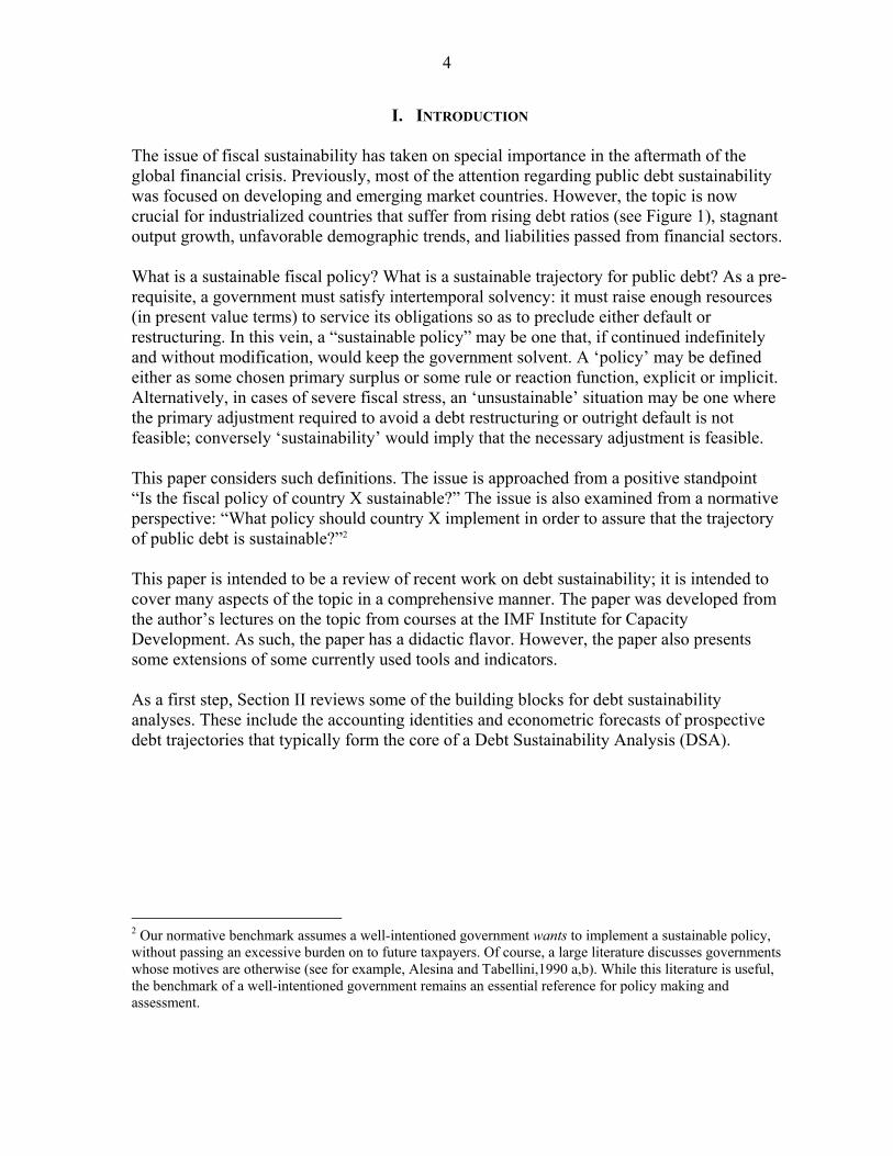
Figures 1. Government Debt/GDP, Selected Countries, Weighted Average ......................................... 5 2. Industrialized Countries: Change in Primary Government Spending (ratio to GDP) 2009
Minus 2008 (vertical axis), and Net Public Debt/GDP (horizontal axis). ........................... 20 3. Emerging Economies: Change in Primary Government Spending (ratio to GDP) 2009
minus 2008 (vertical axis), and Net Public Debt/GDP (horizontal axis) ............................ 21 4. Target Primary Surplus, “Low” Volatility Case ................................................................. 24 5. Target Primary Surplus, “High” Volatility Case ................................................................. 24 References ................................................................................................................................42
4
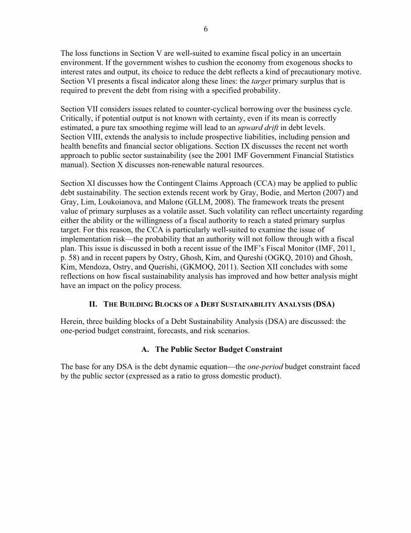
I. INTRODUCTION The issue of fiscal sustainability has taken on special importance in the aftermath of the global financial crisis. Previously, most of the attention regarding public debt sustainability was focused on developing and emerging market countries. However, the topic is now crucial for industrialized countries that suffer from rising debt ratios (see Figure 1), stagnant output growth, unfavorable demographic trends, and liabilities passed from financial sectors. What is a sustainable fiscal policy? What is a sustainable trajectory for public debt? As a pre-requisite, a government must satisfy intertemporal solvency: it must raise enough resources (in present value terms) to service its obligations so as to preclude either default or restructuring. In this vein, a “sustainable policy” may be one that, if continued indefinitely and without modification, would keep the government solvent. A ‘policy’ may be defined either as some chosen primary surplus or some rule or reaction function, explicit or implicit. Alternatively, in cases of severe fiscal stress, an ‘unsustainable’ situation may be one where the primary adjustment required to avoid a debt restructuring or outright default is not feasible; conversely ‘sustainability’ would imply that the necessary adjustment is feasible. This paper considers such definitions. The issue is approached from a positive standpoint “Is the fiscal policy of country X sustainable?” The issue is also examined from a normative perspective: “What policy should country X implement in order to assure that the trajectory of public debt is sustainable?”2 This paper is intended to be a review of recent work on debt sustainability; it is intended to cover many aspects of the topic in a comprehensive manner. The paper was developed from the author’s lectures on the topic from courses at the IMF Institute for Capacity Development. As such, the paper has a didactic flavor. However, the paper also presents some extensions of some currently used tools and indicators. As a first step, Section II reviews some of the building blocks for debt sustainability analyses. These include the accounting identities and econometric forecasts of prospective debt trajectories that typically form the core of a Debt Sustainability Analysis (DSA).
2 Our normative benchmark assumes a well-intentioned government wants to implement a sustainable policy, without passing an excessive burden on to future taxpayers. Of course, a large literature discusses governments whose motives are otherwise (see for example, Alesina and Tabellini,1990 a,b). While this literature is useful, the benchmark of a well-intentioned government remains an essential reference for policy making and assessment.
5
Figure 1. Government Debt/GDP, Selected Countries, Weighted Average
In any analysis of debt sustainability, the size of primary surpluses (revenues minus non- interest expenditures) is critical. As Section III shows, in order to satisfy its intertemporal budget constraint without default, the government must achieve primary surpluses whose present value will be sufficient to cover its debt. Of course, governments are not always able to achieve this goal. Section IV shows how limits on the governments’ ability to run primary surpluses will determine the maximum debt ratio that a country can sustain. In the design of fiscal policy, in addition to the size of primary surpluses, governments must have an objective as to how these primary surpluses would be distributed over time. For example, abrupt changes in the primary surplus from one period to another can introduce undue volatility into macroeconomic aggregates. Moreover, to minimize the overall losses stemming from primary surpluses (including those caused by distorting taxes), the authority should distribute primary surpluses over time in a way that equates marginal losses between periods. Section V discusses alternative specifications for objective functions (loss minimization) and their corresponding fiscal rules that will determine how quickly—if at all—the authority reduces the debt ratio.3
3 This echoes Woodford’s (2003) notion that a rule reflects an underlying optimization process). Consistent with Kydland and Prescott (1977), a fiscal authority that follows a rule which is easy to understand and communicate will gain credibility.
Country coverage/groupings: see the website for the World Economic Outlook, International Monetary Fund. Advanced economies, Euro Area, and United States: debt is reported on a net basis. Emerging / Developing countries: debt is reported on a gross basis.
0
10
20
30
40
50
60
70
80
90
100
19
91
19
92
19
93
19
94
19
95
19
96
19
97
19
98
19
99
20
00
20
01
20
02
20
03
20
04
20
05
20
06
20
07
20
08
20
09
20
10
20
11
20
12
20
13
20
14
20
15
20
16
20
17
Pe
rce
nt
of
GD
P
Public Debt/GDPSource: IMF/WEO
Major advanced economies (G7)
Euro area
Emerging market and developing economies
United States
6
The loss functions in Section V are well-suited to examine fiscal policy in an uncertain environment. If the government wishes to cushion the economy from exogenous shocks to interest rates and output, its choice to reduce the debt reflects a kind of precautionary motive. Section VI presents a fiscal indicator along these lines: the target primary surplus that is required to prevent the debt from rising with a specified probability. Section VII considers issues related to counter-cyclical borrowing over the business cycle. Critically, if potential output is not known with certainty, even if its mean is correctly estimated, a pure tax smoothing regime will lead to an upward drift in debt levels. Section VIII, extends the analysis to include prospective liabilities, including pension and health benefits and financial sector obligations. Section IX discusses the recent net worth approach to public sector sustainability (see the 2001 IMF Government Financial Statistics manual). Section X discusses non-renewable natural resources. Section XI discusses how the Contingent Claims Approach (CCA) may be applied to public debt sustainability. The section extends recent work by Gray, Bodie, and Merton (2007) and Gray, Lim, Loukoianova, and Malone (GLLM, 2008). The framework treats the present value of primary surpluses as a volatile asset. Such volatility can reflect uncertainty regarding either the ability or the willingness of a fiscal authority to reach a stated primary surplus target. For this reason, the CCA is particularly well-suited to examine the issue of implementation risk—the probability that an authority will not follow through with a fiscal plan. This issue is discussed in both a recent issue of the IMF’s Fiscal Monitor (IMF, 2011, p. 58) and in recent papers by Ostry, Ghosh, Kim, and Qureshi (OGKQ, 2010) and Ghosh, Kim, Mendoza, Ostry, and Querishi, (GKMOQ, 2011). Section XII concludes with some reflections on how fiscal sustainability analysis has improved and how better analysis might have an impact on the policy process.
II. THE BUILDING BLOCKS OF A DEBT SUSTAINABILITY ANALYSIS (DSA)
Herein, three building blocks of a Debt Sustainability Analysis (DSA) are discussed: the one-period budget constraint, forecasts, and risk scenarios.
A. The Public Sector Budget Constraint
The base for any DSA is the debt dynamic equation—the one-period budget constraint faced by the public sector (expressed as a ratio to gross domestic product).

7
In any period, the stock of public liabilities tb evolves according to:4
where,
tb = government debt as a ratio to GDP.
ˆ[(1 ) / (1 )]t t tr y
tr = the real rate of interest
ty = the rate of growth of real GDP
t = expenditures on goods and services as a fraction of GDP
t = revenues as a fraction of GDP
This equation says that today’s debt ratio tb equals yesterday’s debt ratio t -1b including both
principal and interest t(1+r ) , but adjusted for the rate of growth of GDPtt(1 + y )ˆ , plus
expenditures t , minus tax revenues t .5 We also assume that the mean interest rate r
exceeds the mean growth rate y ; this is the dynamic efficiency condition.6 The primary surplus is ps . The public sector is assumed to choose some target
primary surplus (ratio to GDP) TAR TAR TARps where TAR is the nominal marginal tax
rate and TAR is the agreed-upon expenditure ratio (as discussed below, this ratio may be viewed as an ex-ante commitment.)
4 Here we refer to the consolidated public sector—the non-financial elements (federal, state, municipal) plus the central bank.
5 We might also include revenues from money creation—the change in real money demand plus inflation tax revenue—in our analysis. While this element has historically been small (typically 1 percent of GDP or less), it became more important during the recent financial crisis—a consequence of quantitative easing. For example, the expansion of the US monetary base in 2008–09 was about 6 percent of GDP. A detailed treatment of revenues from money creation is found in materials developed by Bandiera, Budina, Klijn, and Van Wijnbergen (2007). 6 Long-run considerations of dynamic efficiency imply that the real rate of interest will equal or exceed the
growth rate of real GDP (θ 1). To see why this makes sense, recall that limt ∞ yt 1 r ‐t y0θ‐t yt . This limit term explodes if θ 1. That would imply a future of infinite income. Since income is finite in the present, this is an inefficient outcome. To bring some of this income forward, agents today would consume more and invest less. In so doing, real output growth would fall and the marginal product of capital (linked to the interest rate) would rise. An alternative point of view suggests that the case of θ 1for riskless debt need not be construed as one of dynamic inefficiency or violation of the No Ponzi Game (NPG) condition. A similar point was made by Abel, Mankiw, Summers, and Zeckhauser (1989); see also Blanchard and Weil (2001). More recently, Escolano and others (2011) find that growth plays a relatively small role in keeping θ low. Instead, they find that “The evidence strongly suggests that these low (often negative) real interest rates stem from domestic financial market distortions, captive savings markets, and financial repression.” (emphasis added).
1t t t t tb b (1)
8
In this equation, the error term ste reflects short-run randomness in either the effective tax
rate (changes in the efficiency of the tax system), or expenditures (unauthorized or unfulfilled
planned spending), or both. Note also that, if we substitute TARps into equation (1), we obtain a target value of debt: [ | ]TAR TAR
t t tb E b ps .
B. Ad-Hoc Targets For The Public Debt and/or The Primary Surplus
The algebra that links a chosen primary surplus target TARps and a debt target TARb is simple.
Consider a goal to either stabilize the public debt or reduce it to some target level over anNperiod horizon, written as:
TARt N tb b , where 0 1
A strict inequality implies a goal of debt ratio reduction (not mere stabilization). In this case, Croce and Juan-Ramón (2003) show that the primary surplus must satisfy: For the special case of debt stabilization (a constant debt ratio) ( 1, 1N ) we call the target primary surplus *(1,1)TAR
tps ps . In this case the above is reduced to:
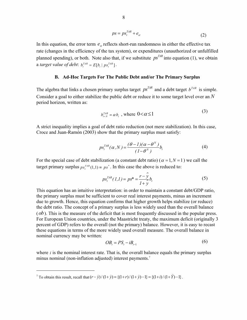
This equation has an intuitive interpretation: in order to maintain a constant debt/GDP ratio, the primary surplus must be sufficient to cover real interest payments, minus an increment due to growth. Hence, this equation confirms that higher growth helps stabilize (or reduce) the debt ratio. The concept of a primary surplus is less widely used than the overall balance ( ob ). This is the measure of the deficit that is most frequently discussed in the popular press. For European Union countries, under the Maastricht treaty, the maximum deficit (originally 3 percent of GDP) refers to the overall (not the primary) balance. However, it is easy to recast these equations in terms of the more widely used overall measure. The overall balance in nominal currency may be written: where i is the nominal interest rate. That is, the overall balance equals the primary surplus minus nominal (non-inflation adjusted) interest payments.7 7 To obtain this result, recall that ( ) / (1 ) {(1 ) / (1 ) 1} {(1 ) / (1 ) 1}r y y r y i Y
.
TARt stps ps e
NTARt tN
( 1)( )ps ( ,N ) b
(1 )
TARt t
r yps (1,1) ps* b
1 y
1t t tOB PS iB
(2)
(3)
(4)
(5)
(6)
9
If inflation rises, investors are compensated through higher nominal interest rates. As a fraction of GDP, the overall balance that is required to stabilize debt *ob is thus: Even if the primary surplus must be positive to stabilize the debt, the overall balance may be in deficit—so long as growth is positive.8 However, the primary surplus ps is a more
meaningful indicator of fiscal adjustment than the operational balanceob : two different
countries may have the same value for *ob but different values for *ps , owing to different
values of i , Y
, or 1tb .
C. Alternative Scenarios in a Debt Sustainability Analysis
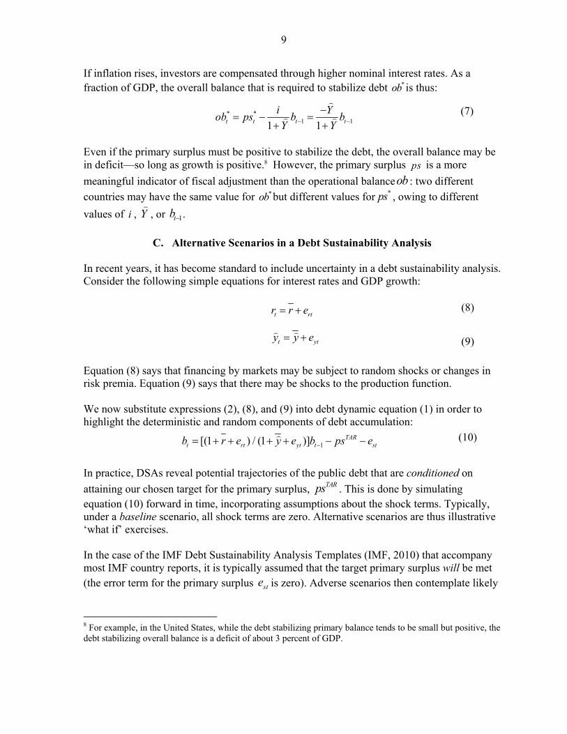
In recent years, it has become standard to include uncertainty in a debt sustainability analysis. Consider the following simple equations for interest rates and GDP growth: Equation (8) says that financing by markets may be subject to random shocks or changes in risk premia. Equation (9) says that there may be shocks to the production function. We now substitute expressions (2), (8), and (9) into debt dynamic equation (1) in order to highlight the deterministic and random components of debt accumulation: In practice, DSAs reveal potential trajectories of the public debt that are conditioned on
attaining our chosen target for the primary surplus, TARps . This is done by simulating equation (10) forward in time, incorporating assumptions about the shock terms. Typically, under a baseline scenario, all shock terms are zero. Alternative scenarios are thus illustrative ‘what if’ exercises. In the case of the IMF Debt Sustainability Analysis Templates (IMF, 2010) that accompany most IMF country reports, it is typically assumed that the target primary surplus will be met (the error term for the primary surplus ste is zero). Adverse scenarios then contemplate likely
8 For example, in the United States, while the debt stabilizing primary balance tends to be small but positive, the debt stabilizing overall balance is a deficit of about 3 percent of GDP.
t rtr r e
t yty y e
1[(1 ) / (1 )] TARt rt yt t stb r e y e b ps e
* *1 11 1t t t t
i Yob ps b b
Y Y
(7)
(8)
(9)
(10)

10
shocks to output, interest rates, or both. The adverse shocks ( rte >0, yte <0) are typically two
standard deviations from their (zero) mean. More recently, several authors have developed methods involving stochastic Monte Carlo simulations of equation (10). These simulations, which are summarized in Table 1, tell us the probability that our debt will equal or exceed some debt target TAR
t tb b .
Table 1. Summary, Recent Research on Public Debt Sustainability, Stochastic Approach
Author(s) Year Country(s) Remarks Hunt, Drew 1998 New Zealand Hoffmaister, others 2001 Costa Rica Garcia, Rigobon 2004 Brazil Penalver, Thwaites 2006 Emerging Markets Celasun, Debrun, Ostry 2007 Emerging Markets Fiscal Reaction Function Tanner,Samake 2008 Brazil, Mexico, Turkey Congressional Budget Office 2008 United States Budina, Van Wijnbergen 2009 Turkey Includes seignorage forecasts
Frank, Ley 2009 Argentina, Brazil, S. Africa Regime changes (Markov switching model)
Hadjenberg, Romeu 2010 Uruguay Includes parameter uncertainty Kawakami, Romeu 2011 Brazil Fiscal Reaction Function
Early efforts to simulate the future evolution of government debt were based on empirical estimates of interactions between fiscal and real variables (including vector autoregressions technique), which include Hunt and Drew (1998, New Zealand), Hoffmaister and others (2001, Costa Rica), and Garcia and Rigobón (2004, Brazil).9 The papers by Penalver and Thwiates (2006) and Celasun, Debrun, and Ostry (CDO, 2007) both develop a vector autoregression analysis of public debt in emerging markets. CDO includes a fiscal reaction function wherein primary surpluses respond to the debt level itself. Both CDO and Tanner and Samake (2008, Brazil, Mexico, Turkey) simulate the primary surplus that is required to stabilize or reduce the debt for specific probabilities. For the United States, a detailed ‘fan chart’ analysis is presented by the Congressional Budget Office (CBO, 2007). Budina and Van Wijnbergen present an analysis of Turkey’s fiscal sustainability that also includes assumptions regarding inflation and revenue from money creation. Frank and Ley (2009, Argentina, Brazil, and South Africa) depart from most of the literature by considering both regime changes (modeled by a Markov-switching routine) and abnormal distributions. More recently, Hadjenberg and Romeu (2010, Uruguay) examine the
9 As an alternative strategy, Hostland and Karam (2005–06) examine the issue of debt sustainability in a calibrated New-Keynesian model.
11
effects of parameter uncertainty (as well as shocks) on debt projections. Kawakami and Romeu (2011, Brazil) identify fiscal transmission and a fiscal policy reaction functions within a debt projection framework.
III. THE GOVERNMENT’S PRESENT VALUE CONSTRAINT: A RESTATEMENT
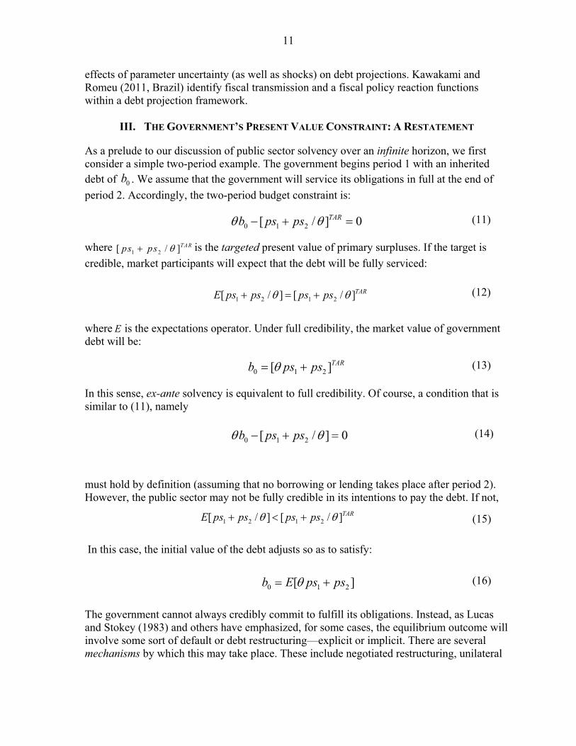
As a prelude to our discussion of public sector solvency over an infinite horizon, we first consider a simple two-period example. The government begins period 1 with an inherited debt of 0b . We assume that the government will service its obligations in full at the end of
period 2. Accordingly, the two-period budget constraint is: where
1 2[ / ]TARps ps is the targeted present value of primary surpluses. If the target is
credible, market participants will expect that the debt will be fully serviced: where E is the expectations operator. Under full credibility, the market value of government debt will be: In this sense, ex-ante solvency is equivalent to full credibility. Of course, a condition that is similar to (11), namely must hold by definition (assuming that no borrowing or lending takes place after period 2). However, the public sector may not be fully credible in its intentions to pay the debt. If not, In this case, the initial value of the debt adjusts so as to satisfy: The government cannot always credibly commit to fulfill its obligations. Instead, as Lucas and Stokey (1983) and others have emphasized, for some cases, the equilibrium outcome will involve some sort of default or debt restructuring—explicit or implicit. There are several mechanisms by which this may take place. These include negotiated restructuring, unilateral
0 1 2[ / ] 0TARb ps ps
0 1 2[ ]TARb ps ps
0 1 2[ / ] 0b ps ps
0 1 2[ ]b E ps ps
1 2 1 2[ / ] [ / ]TARE ps ps ps ps
1 2 1 2[ / ] [ / ]TARE ps ps ps ps
(11)
(12)
(13)
(14)
(15)
(16)

12
defaults, or inflation. Typically, none of these options are benign; governments make substantial efforts to avoid them.10 We next generalize to an infinite horizon. A government satisfies its intertemporal solvency or No Ponzi Game (NPG) condition if: Note that the debt ratio may be expressed as: where B
is the growth rate of nominal debt and Y
is the growth rate of nominal GDP. Thus,
NPG is satisfied so long as (1 ) / (1 ) (1 )B Y r
.11 As with the finite horizon case, condition (17) always holds ex-post. Ex-ante, the government is solvent so long as the present value of targeted primary surpluses credibly satisfies condition (17). It is possible for the debt ratio to rise ( B Y
) and still comply ex-ante with the NPG condition. However, for
this to happen, the primary surplus ps must also continually rise according to a continuous fiscal rule: 10 Regarding inflation, the ‘Fiscal Theory of the Price Level’ (FTPL), as discussed by Cochrane (1998), Woodford (2001), and others, is a recent idea in the economics literature. According to the FTPL, higher inflation reduces the real value of government debt (as if it were an equity share). However, as Kumhof and Tanner (2008) emphasize, most governments permit such a remedy only as a last resort, since a default (through inflation or otherwise) can have detrimental impacts on financial systems. 11 Thus, the growth rate of debt
1ˆ / 1t tB B B is determined both by the primary surplus (a policy choice) and
the interest rate. An alternative formulation of the NPG condition, in which the interest rate must exceed the growth rate, is:
1
1
/ tt t
t
b ps
Here, the NPG condition is lim / 0ttt
b
. This condition is more restrictive. It tells us that growth of debt
cannot exceed the interest rate. However, this condition is uninformative about cases where debt growth exceeds output growth. As McCallum (1983) suggested, there are cases where the debt ratio can grow but the NPG condition still holds. McCallum emphasized – and we agree – that such cases are typically only of theoretical interest since the government may not be able to credibly commit to the ever-increasing primary surpluses that such a policy would demand.
1lim / (1 ) 0tt
tb r
1, 0TAR TAR TARt tps b
0
0
(1 )
(1 )
t
tt t
t
B B Bb
Y Y Y
(17)
(18)
(19)
13
or desired response of the primary surplus to the debt. Sustainability requires TAR >0; this point was emphasized by Bohn (1998, 2008); more recently Escolano (2010) and Ostry and others (2010) noted that at high ratios of debt, at some point the required target primary
surplus TARps may be infeasible; we discuss this case in the next section. Importantly, a
policy for which TARps may remain constant and still satisfy the NPG condition is one of debt stabilization, namely B Y
. Of course, this policy implies that ( ) / (1 ) *TAR
t tps r y y b .
IV. MAXIMUM SUSTAINABLE DEBT
For the average citizen of a country, it may be difficult to link in a precise way the level of debt to their own well-being. By contrast, the primary surplus is more easily understood by citizens: they directly suffer when their taxes are raised and when important expenditures are cut.12 Even so, discussions of fiscal sustainability are often phrased in terms of debt levels: “What is the maximum sustainable (or ‘tolerable’) debt level that a country can support?”13 One way to answer this question was suggested by Mendoza and Oviedo (2006) and Escolano (2010). They begin with some maximum feasible primary surplus that citizens can
tolerate. We may call this level maxps . If so, the maximum debt ratio is easily obtained by inverting expression (5) and substituting in the maximum primary surplus, so as to obtain
maxb That is, the maximum debt is simply the annuity value of the maximum primary surplus
(adjusted for real GDP growth). If max
b b a restructuring of the public debt may be a
desirable outcome; the condition * maxps ps implies that adjustment is not politically feasible. Market participants often compare the maximum sustainable debt ratios of different countries. This framework yields a clear way to do so. Consider countries, I and II:
12 There is an analogy for monetary policy and inflation. For the average citizen, alternative measures of the money supply may be mysterious. However, inflation is tangible and understandable.
13 The idea of ‘debt intolerance’ was introduced by Reinhart, Rogoff, and Savastano (2003). The logic presented in this section is consistent with International Monetary Fund’s indicators for maximum sustainable debt (2004, p. 21).
( ) ( )max maxb I b II (21)
max maxˆ ˆ[(1 ) / ( )]b y r y ps (20)
14
This implies that,
Thus, a country that grows faster, with all else equal, can sustain a higher debt ratio. Likewise, fiscal institutions matter. Countries with broader tax bases, more efficient tax administration systems, less tax evasion, and more productive expenditures (list of factors not exhaustive) can generate a higher maximum primary surplus whose impact on growth is less detrimental. 14
Markets typically distinguish between countries on the basis of their institutions and their growth. Expression (22) shows that, to be credible, fiscal consolidations often must include reforms (i.e. of tax collection and administration, base broadening, and, more broadly, elimination of counterproductive regulations). Such measures can effectively raise the maximum (or ‘tolerable’) level of public debt.
V. DISTRIBUTING SURPLUSES OVER TIME: A FISCAL OBJECTIVE FUNCTION The previous two sections focused on the size of the primary surpluses that the government must run in order to satisfy its in—tertemporal constraint without default or restructuring. However, there is another key objective that governments must consider in designing a sustainable fiscal policy: how these primary surpluses are distributed over time. To develop an objective function, our starting point is the tax smoothing objectives of Barro (1979) and Sargent (1987)—how to spread the deadweight losses of taxation (or primary surpluses) over time.15 A related concern is that the volatility fiscal policy may introduce into the economy. For example, a delayed fiscal adjustment—low taxes today, higher taxes in the future—means additional volatility, even if taxes are lump sum.16 Here, we consider an objective function that is similar in spirit to Barro (1979) but is more general. That objective will yield policy rules that are simple and easily communicated to the public—as Kydland and Prescott (1977) suggested.
14 Simulations by Altig et. al. (2001) suggest that base broadening and other tax reforms can substantially boost growth.
15 The idea of tax smoothing continues to receive attention in the optimal fiscal policy literature; see, for example Kingston (1991), Lloyd-Ellis, Zhan, and Zhu (2005), and Fisher and Kingston (2005). While Lucas and Stokey (1983) broadened the discussion to include optimal sovereign defaults, that outcome is not emphasized in this paper.
16 Of course, governments may vary tax rates countercyclically. Doing so may reduce volatility—so long as the countercyclical policy is in fact symmetric (low taxes during recession must be offset by higher taxes in the future).
(22) max maxˆ ˆ ˆ ˆ[(1 ) / ( )] [(1 ) / ( )]I I I I II II II IIy r y ps y r y ps

15
A. Objective: How To Distribute The Fiscal Burden Over Time
A policy objective is to minimize the present value of expected deadweight losses associated with tax collection, subject to the intertemporal budget constraint. The loss function is:
where ' ''0, 0 . Regarding the third moment, we consider two cases: (i) ''' 0 and (ii): ''' 0 . For a minimum, the first order (Euler) condition must hold:
Case (i): Barro-Sargent Tax-Smoothing
If ''' 0 or if there is no volatility 21( ) 0t tE equation (24) reduces to:
Under certainty, we can drop expectations. This is Barro’s 1979 tax smoothing result.17 The expression has a simple, appealing intuition. A benevolent fiscal authority should aim to equate the marginal costs of tax collection across periods. When it distributes costs in this way, the authority favors neither the present nor future. However, expression (25) does not tell us what the optimal tax rate is—only that the optimal tax rate should be (on average) equal across periods. To obtain the optimal tax rate * t
, we
must take expression (25) and substitute it into budget constraint (17). Doing so yields: Since t t tps , equation (26) is simply a restatement of equation (5). This result has an
appealing implication. At first glance, a rule to stabilize the debt might have been considered either arbitrary or naïve. It is now seen to flow from a specific objective function. It is also an easily communicated rule: “Our objective is to stabilize the debt—and hence primary
17 In Sargent’s 1987 extension of Barro’s model, a quadratic loss function was assumed: 2( )t t . In this
case, the first order condition for the current and future periods (t, t+1) are respectively: 2 t and
12 / /t , where is a Lagrange multiplier. The tax smoothing result is obtained by combining these
two first order conditions.
1
1
[ ( ) ]tt
t
L E
' '1( ) ( ( ))t tE
1( )t tE
(23)
(24)
(25)
(26) *t t t 1
ˆr yb
ˆ1 y

16
surpluses. In so doing, we are neither favoring current nor future tax payers; we are safeguarding future tax payers against a higher tax burden”. However, this rule is unappealing in some ways. First policy is invariant to volatilities of , r and y
. No matter how uncertain the economic environment is, the policy rule will be the
same. There is no precautionary element that directs the fiscal authority to ‘save for a rainy day’ if volatility increases. Second, the policy rule has a symmetric property: a 5 percent increase of the debt ratio offsets a 5 percent decrease. But, this symmetry is inconsistent with typical DSA graphs that show adverse risk scenarios—but not favorable ones. For a policy-maker whose preferences are case (i) of equation (22) such adverse scenarios would be of no interest.
Case (ii): A prudent fiscal authority ( ''' 0 ). If adverse scenarios are shown, as is the case in most DSAs, it is because policymakers are interested in preventing such scenarios. In this sense, a loss function with a third moment—something absent from case (i) but present in case (ii)—would better characterize an authority’s preferences.18 To further examine case (ii), it would be helpful to write the fiscal burden in any period as the sum of primary expenditures and interest payments (adjusted for economic growth):
1t t tfb rb , where ( ) / (1 )r r y y is the growth-adjusted interest rate. In each period,
the prospective variability of the tax burden is 21( )t tE .
The budget constraint says that this term must be linked to the variance of the fiscal burden, which may be written as: The first term on the right hand side tells us that there is variability linked to primary spending but unrelated to the debt level. The second term tells us that, through changes in interest rates and growth rates, there is an element of fiscal variability that is linked to the stock of debt—higher debt means more variability. The third term is a covariance term; for this exposition, it is assumed to be zero. Substituting the variance of the fiscal burden into expression (24) and taking a second-order Taylor approximation yields:19 18 Our emphasis on the third moment is analogous to the analysis of precautionary saving found in authors like Blanchard and Fischer (1989, p.289), Caballero (1990), Kimball (1990), Carroll and Kimball (1996), and others. The second-order approximation used in this section is developed by Talmain (1998) and Gourinchas and Parker (2002). Hugget and Ospina (2001) note that, for precautionary saving to be observed in the aggregate, a third moment of the utility function is not required.
19 Analyses that are based on Taylor expansions of the Euler equation should be considered here as a useful heuristic, since they use approximations that are valid for small deviations from an initial steady state. Even so, as Talmain (1998) shows, the errors inherent in such approximations can be small.
2 2 21 1 1 1 1( ) ( ) ( ) 2 ( )( )t t t t t t t t t tE fb fb E E rb rb E rb rb (27)
17
Equation (28) confirms that stochastic simulation exercises (see Part II) are of interest under case (ii) but irrelevant for case (i). Equation (28) also shows that there are two elements to the prudential element of taxes. The first element 2
1( )t t may be thought of as budgetary
risks—unexpected or unauthorized spending. The second element 21( )t trb rb may be
thought of as financial risks. If 21( ) 0t tE , this second element would exclusively
reflect unexpected changes to financing costs (the interest rate). In this special case, the fiscal rule would take the form: where 0 is derived from the function . Under this rule, in the long-run, the debt tends to zero. A simple one-period example shows how tax-smoothing rule (26) is a special case of rule (29). Assume an initial debt ratio 0 50 percentb , average growth y
equal to 3 percent
and the real interest rate requal to 12 percent. Assume also that the standard deviation of ( ) / (1 )r y y
is 1 percent and the distribution is standard normal. Under rule (25), the
primary surplus chosen by the authority would be * 4.4 percentps . Implicitly, this means that the fiscal authority would be willing to take a 50 percent risk that debt rises—requiring another adjustment. Under a rule like (29), if the authority aims to limit that risk to 15
percent, it should target a primary surplus ** 4.9 percentps of GDP. In so doing, the authority has signaled a willingness to pay an extra 0.4 percent of GDP so as to reduce the risk of another adjustment from 50 percent to 15 percent. Like tax smoothing, this objective can also be easily communicated: “Our objective is to adjust now so as to avoid another fiscal adjustment for all but the worst w-percent of cases. As a byproduct, we also reduce debt to zero”. A modified rule emerges if we instead assume that budgetary risks are present and constant:
21( )t tE const . Through the debt dynamic equation, such risks will also affect the
second element 21( )t trb rb —even if there are no interest rate shocks.
In this case, our more general rule includes a constant structural surplus:
**t t
r yps [ ]b
1 y
'''2 2
1 1 1''
( )( ) {.5* *[ ( ) ( ) ] ...}
( )t
t t t t t tt
E E E rb rb
SSt t
r yps ps [ ]b
1 y
(28)
(29)
(30)

18
where 0ps is the structural primary surplus as a fixed percent of GDP and 0 .20 Since the structural surplus is positive, the country will be a net creditor in the long run. Substitution of (30) into budget constraint (1) in any period t yields: 1(1 )t tb b ps
Overtime, the government accumulates assets. Its bounded net credit position converges to: Such a bound is desirable. Otherwise, the government, as an owner of private assets, may have excessive influence in the private economy.21
B. Objective Functions and Structural Surpluses—Further Considerations
In recent years, economists have emphasized that policies should be conducted so as to maximize consumer welfare. This idea draws on Frank Ramsey’s (1927) concept of a benevolent planner.22 Under this approach, the planner acts to directly maximize consumer utility functions rather than some ad-hoc objective function.23 Even so, an ad-hoc objective function may reflect the underlying welfare of consumers. As one example, assume that the expected present value of the utility of the representative consumer is:
where we assume that ' '' '''0, 0, 0U U U . Consider a steady state for a ’hand-to-mouth’ (or credit-constrained) consumer with no assets, where income is fixed and known (
1,t t tY Y
) and the subjective rate of discount equals the (gross) rate of interest (1 )r ; for this
consumer, (1 ).t t t t tC Y T Y
20 Garcia, Restrepo, and Tanner (2011) discuss the case of Chile, where ps was initial 1 percent of GDP, but
was reduced to ½ of 1 percent in the early 2000s.
21 There are two reasons why we would not expect to have a rule with 0ps but 0 . First, as mentioned
above, budgetary risks will also be reflected in financial risks; the two risks are inherently connected through the debt dynamic equation. Second, such a policy implies boundless asset accumulation.
22A seminal paper in this literature (Chari, Christiano, and Kehoe, 1994) finds that policy which satisfies this optimality criteria may not always coincide with a tax-smoothing objective. 23 Some authors have examined fiscal objective functions in general equilibrium simulations. See Kumhof and Yakadina (2007), for example.
lim /ttb ps
1
1
[ ( ) ]tt
t
U E U C
(31)
(32)
(33)
19
As before, we assume that the variability of taxes is linked to the variability of the fiscal burden. In this case, the Euler equation ' '
1( ) ( )t tU C U C (for ) yields an expression
similar to (28): Since ''' ''/ 0U U , equation (34) says that as the variability of the fiscal burden rises, taxes need to be ‘front loaded’. This result is consistent with objective (23) and fiscal rules like (29) or (30), but it is measured in terms of units of consumption. It is also similar to Garcia, Restrepo, and Tanner (2011), who consider a case in which exogenous revenues come from a natural resource (copper). In this case, expenditures should be optimally tilted upwards. Using a Constant Relative Risk Aversion (CRRA) utility function, they derive an optimal fiscal rule similar to (30). Note also that, if taxes were lump-sum, only hand-to-mouth consumers would care about the time path of taxes. Consumers who do enjoy access to capital markets—Ricardian consumers—would be able to smooth consumption on their own. A structural surplus provides a way to implement the recommendation of Aiyagari, Marcet, Sargent, and Seppala (AMSS, 2002) for the government to accumulate a “war chest” of assets so as to avoid the need for distortionary tax financing of primary government surpluses.24 The importance of such a “war chest” to reduce macroeconomic volatility is discussed in the next section.
C. Debt and Expenditure Smoothing—Evidence From the Recent Downturn
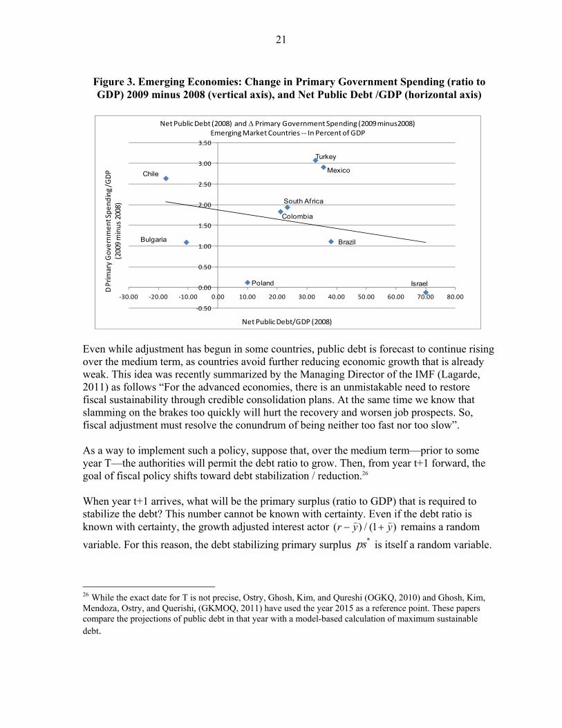
Prior to the recent financial crisis, one might have dismissed the ‘war chest’ idea as a mere debating point. In the aftermath of the recent crisis, such an idea has taken on greater importance. Evidence suggests that countries with lower debt ratios—and especially those few countries whose public sector were net creditors—were better positioned to respond to the economic downturn with countercyclical increases in their non-interest public expenditures. Figures 2 and 3 illustrate this point. For industrialized and emerging market countries respectively, these figures plot debt ratios in 2008 against the change in the primary surplus/ GDP ratio 2009 minus 2008 ( / (2009 – 2008)G GDP ). A more positive number indicates a higher spending ratio in 2009 relative to 2008—a more countercyclical policy.
24 Note that the link between AMSS (2002) and our rule is approximate. They recommend that the governments’ net credit position be equal to the perpetuity value of government purchases / r . Doing so
permits the government to set taxes to zero. Also, the rationale behind AMSS is to eliminate the deadweight losses of distortionary taxes. Because we consider hand-to-mouth consumers, we are concerned with volatility – which includes lump-sum taxes. Moreover, this approach provides an extra margin of security that countercyclical safety net expenditures will not be cut during a severe recession – “a safety net for the safety net”.
'''
1 1''( ) .5 ( )* var( ) ...t t
UT E T C fb
U (34)

20
Among these two groups, there are several examples of countries that had net credit position: Finland and Norway (industrialized countries) and Bulgaria and Chile (emerging market countries). Of these, all but Bulgaria also posted substantial increases in public spending ratios (a more countercyclical policy). The chart also displays several cases wherein higher debt was coupled with a less countercyclical fiscal policy (lower increases in the spending ratio). Amongst industrialized countries, this group includes Switzerland, Italy, Greece, and Japan; amongst emerging market countries, Israel with relatively high debt that posted a fall in its public spending ratio.25
VI. REQUIRED ADJUSTMENT IN AN UNCERTAIN ENVIRONMENT
The recent global economic crisis has put severe strains on fiscal balances in many countries. Cyclical factors, automatic stabilizers, countercyclical expansions, and support for financial sectors have contributed to rising public debt ratios over the medium-term.
Figure 2. Industrialized Countries: Change in Primary Government Spending (ratio to GDP) 2009 Minus 2008 (vertical axis), and Net Public Debt /GDP
(horizontal axis).
Source: IMF WEO
25 For both industrialized and emerging markets, the slope coefficient is estimated to be negative; for industrialized countries, the t-statistic is about 2.9. Since there are few data points, the empirical analysis is intentionally informal.
Austria
BelgiumCanada
Denmark
Finland
France
Germany Greece
Iceland
Italy
Japan
Luxembourg
Netherlands
Norway
Spain
Switzerland
United Kingdom
United States
0.75
1.75
2.75
3.75
4.75
5.75
6.75
7.75
-150 -100 -50 0 50 100 150
Net Public Debt (2008) and Primary Government Spending (2009 minus 2008)Industrialzed Countries -- In Percent of GDP
Net Public Debt/GDP (2008)
D P
rim
ary
Go
vern
me
nt S
pe
nd
ing
/GD
P
(200
9 m
inu
s 20
08)
Source: IMF/WEO
21
Source: IMF WEO
Even while adjustment has begun in some countries, public debt is forecast to continue rising over the medium term, as countries avoid further reducing economic growth that is already weak. This idea was recently summarized by the Managing Director of the IMF (Lagarde, 2011) as follows “For the advanced economies, there is an unmistakable need to restore fiscal sustainability through credible consolidation plans. At the same time we know that slamming on the brakes too quickly will hurt the recovery and worsen job prospects. So, fiscal adjustment must resolve the conundrum of being neither too fast nor too slow”. As a way to implement such a policy, suppose that, over the medium term—prior to some year T—the authorities will permit the debt ratio to grow. Then, from year t+1 forward, the goal of fiscal policy shifts toward debt stabilization / reduction.26 When year t+1 arrives, what will be the primary surplus (ratio to GDP) that is required to stabilize the debt? This number cannot be known with certainty. Even if the debt ratio is known with certainty, the growth adjusted interest actor ( ) / (1 )r y y
remains a random
variable. For this reason, the debt stabilizing primary surplus *ps is itself a random variable. 26 While the exact date for T is not precise, Ostry, Ghosh, Kim, and Qureshi (OGKQ, 2010) and Ghosh, Kim, Mendoza, Ostry, and Querishi, (GKMOQ, 2011) have used the year 2015 as a reference point. These papers compare the projections of public debt in that year with a model-based calculation of maximum sustainable debt.
BrazilBulgaria
Chile
Colombia
Israel
Mexico
Poland
South Africa
Turkey
-0.50
0.00
0.50
1.00
1.50
2.00
2.50
3.00
3.50
-30.00 -20.00 -10.00 0.00 10.00 20.00 30.00 40.00 50.00 60.00 70.00 80.00
Net Public Debt (2008) and Primary Government Spending (2009 minus2008)Emerging Market Countries -- In Percent of GDP
Net Public Debt/GDP (2008)
D P
rim
ary
Go
vern
me
nt S
pe
nd
ing
/GD
P
(200
9 m
inu
s 20
08)
Figure 3. Emerging Economies: Change in Primary Government Spending (ratio to GDP) 2009 minus 2008 (vertical axis), and Net Public Debt /GDP (horizontal axis)
22
If the growth adjusted discount factor is distributed normally, then the debt stabilizing primary surplus will also be so distributed; its mean will be [( ) / (1 )]*mean r y yb
and its standard deviation will be . [( ) / (1 )]*std dev r y yb
.
Under these assumptions, ( )TARps x the target values for primary surplus that would be required to prevent the debt from rising above its year (t) forecast with an x-percent
probability ( )TARps x would be defined as:
where *[ ]1
r y
yps mean b
.27
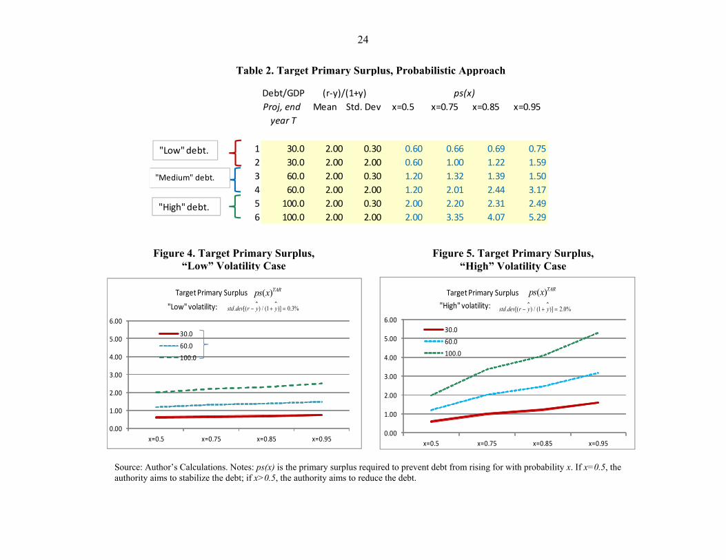
Table 2 and Figures 4a and 4b present such calculations for six hypothetical countries. Countries 1 and 2 have a “low” debt ratio (30 percent of GDP); countries 3 and 4 have a “medium” debt ratio (60 percent of GDP); countries 5 and 6 have a “high” debt ratio (100 percent of GDP). In all cases, the level of the growth adjusted interest factor is equal to 2 percent. Within each group, countries are distinguished by the volatility (standard deviation) of that factor. In the “low volatility” countries the standard deviation of that factor is 0.3 percent; in the “high” volatility countries, that standard deviation is 2.0 percent. In each case,
the target primary surplus ( )TARps x is calculated for values of x = 0.5, 0.75, 0.85, and 0.95. Results for the “low” volatility cases are shown in Figure 4a and for the “high” volatility cases in Figure 4b. As one example, if country 1 ran a primary surplus of 0.6 percent of GDP in year T+1, the probability that the debt would continue to rise would be 50 percent (x=0.5). In order to reduce that probability to 25 percent (x=0.75), the authorities would have to raise the primary surplus another 0.06 percent of GDP to 0.66 percent; to reduce that probability to 15 percent (x=0.85), the primary surplus would have to increase to 0.69 percent of GDP; to reduce that probability to 5 percent (x=0.95), the primary surplus would have to increase to 0.75 percent of GDP. The results confirm that higher primary surpluses are required if either the debt level or the growth adjusted discount factor increase. They also confirm that a more ‘prudent’ authority—one whose objective is to reduce the probability that the debt will rise (higher x)—will also run a higher primary surplus than a less prudent authority. However, Table 2 and Figures 4a-b convey two other important messages. First, an increase in volatility (higher standard deviation of growth adjusted interest factor) makes it even more
27 This formulation has a ‘value at risk’ (VaR) interpretation that is similar to Kopits and Barnhill (2003) and Tanner and Carey (2008). This expression can be directly linked to the theoretical formulation in the previous section. The implied prudence factor, as discussed ''' ''/ ( )implied is simply calculated as the ratio
[ ] [ ]1 1
[ ( ) ] / 0.5* varTAR r y r y
y yps x mean b b
.
*( ( ) )TARPR ps x ps x
(35)
23
difficult for a government to reduce the probability that its debt will grow. This is indicated by lines that are more steeply sloped in Figure 4b than in Figure 4a. Second, a combination of high debt ratios and high volatility can pose yet even more difficulties for the objective of debt stabilization. This is illustrated in Figure 4b: as debt levels rise, so do the slopes of their respective lines; the most steeply sloped line is the one that shows ps(x)TAR for the “high” debt country (b=100 percent of GDP). Hence, these calculations confirm that economic volatility is the enemy of fiscal sustainability. For countries that suffer from exogenous volatility, it is important to restrain debt. However, eliminating or reducing domestic sources of volatility—erratic monetary policies, poorly functioning financial markets, and undue variations in tax revenues and expenditures—will also support the objective of fiscal sustainability.
VII. SUSTAINABILITY OVER THE BUSINESS CYCLE 28
The primary surplus is sensitive to the business cycle. It contains both a structural element
( ) Pt P tps struc y where P
ty is trend (or potential) output and the cyclical component is
, ,( ) ( ) ( )( )P Pt c t t c TAX c SPEND t tps cyc y y y y , where ,c TAX ,c SPEND are cyclical
elasticitites for taxes and expenditures, respectively. The total primary surplus is:( ) ( )t t tps ps struc ps cyc .
Typically, , 1c TAX . Net tax revenues (including transfers) typically fall during a recession
and rise during an expansion. By contrast, ,c SPEND will be zero if governments smooth their
expenditures (much like a private household would do if it obeyed the permanent income hypothesis). In this analysis, the debt will be stabilized if two conditions hold. First, the structural surplus must correspond to its debt stabilizing value: *( ) tps struc ps . This is the tax smoothing
regime—equation (26). Under this regime, governments will borrow during downturns, and reduce debt during recoveries. So long as deficits and surpluses fully cancel out over time, government debt will be stabilized. A second critical assumption is that the government knows what P
ty is—with certainty. If
potential output is uncertain, even if *( ) tps struc ps if potential output is uncertain and the
government implements tax smoothing regime (26), the debt ratio will drift upward even if the mean of Py is correctly estimated. To see why, consider the example that is summarized
in Table 3. Suppose that initial potential output is equal to actual output equal to 100
28 This section is based on Tanner and Carey (2008). Discussions of how to compute the cyclically adjusted fiscal balance are found in Girouard and ndré (2005) and Fedelino, Ivanova, and Horton (2009).
24
Debt/GDP
Proj, end year T
Mean Std. Dev x=0.5 x=0.75 x=0.85 x=0.95
1 30.0 2.00 0.30 0.60 0.66 0.69 0.75
2 30.0 2.00 2.00 0.60 1.00 1.22 1.59
3 60.0 2.00 0.30 1.20 1.32 1.39 1.50
4 60.0 2.00 2.00 1.20 2.01 2.44 3.17
5 100.0 2.00 0.30 2.00 2.20 2.31 2.49
6 100.0 2.00 2.00 2.00 3.35 4.07 5.29
(r-y)/(1+y) ps(x)
"Low" debt.
"Medium" debt.
"High" debt.
0.00
1.00
2.00
3.00
4.00
5.00
6.00
x=0.5 x=0.75 x=0.85 x=0.95
30.0
60.0
100.0
0.00
1.00
2.00
3.00
4.00
5.00
6.00
x=0.5 x=0.75 x=0.85 x=0.95
30.0
60.0
100.0
"High" volatility:
Target Primary Surplus Target Primary Surplus
"Low" volatility: . [( ) / (1 )] 0.3%std dev r y y . [( ) / (1 )] 2.0%std dev r y y
( )TARps x ( )TARps x
Source: Author’s Calculations. Notes: ps(x) is the primary surplus required to prevent debt from rising for with probability x. If x=0.5, the authority aims to stabilize the debt; if x>0.5, the authority aims to reduce the debt.
Table 2. Target Primary Surplus, Probabilistic Approach
Figure 5. Target Primary Surplus, “High” Volatility Case
Figure 4. Target Primary Surplus, “Low” Volatility Case
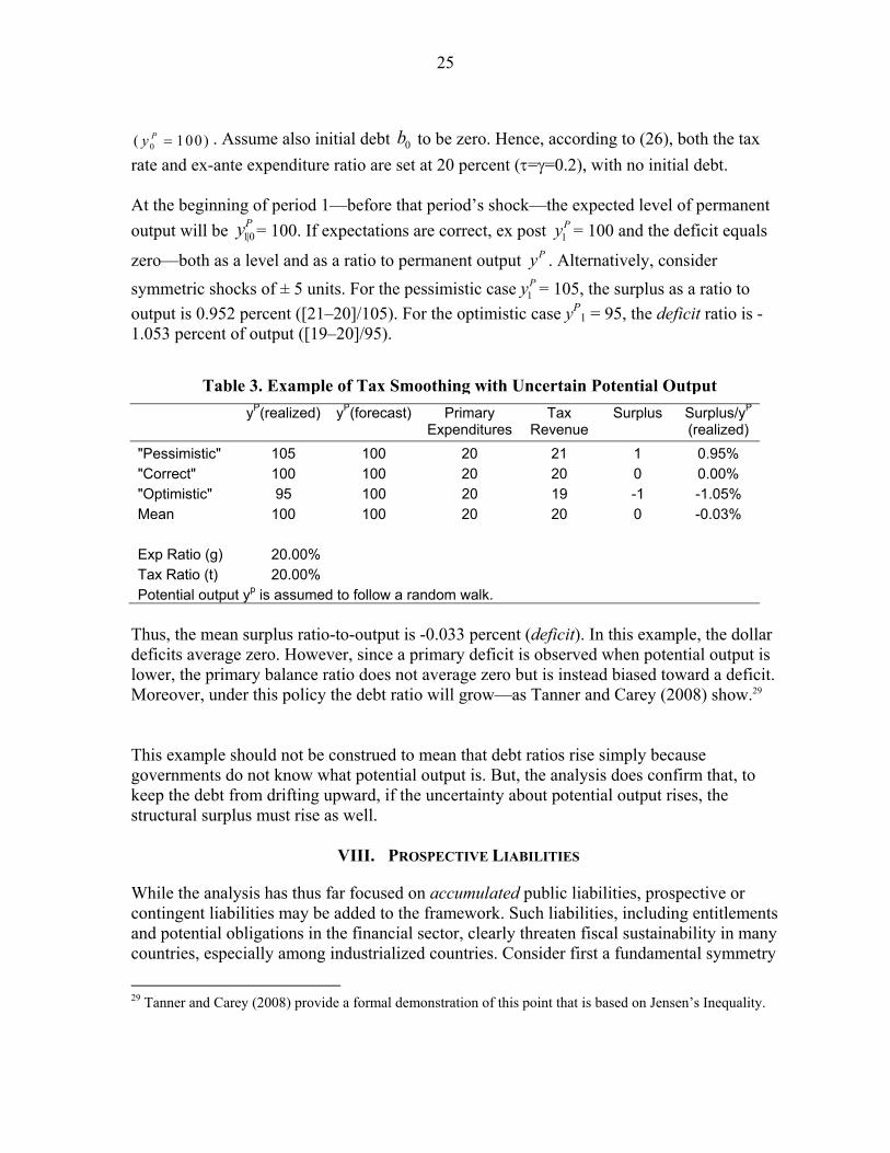
25
0( 100)Py . Assume also initial debt 0b to be zero. Hence, according to (26), both the tax
rate and ex-ante expenditure ratio are set at 20 percent (==0.2), with no initial debt. At the beginning of period 1—before that period’s shock—the expected level of permanent
output will be 1|0Py = 100. If expectations are correct, ex post 1
Py = 100 and the deficit equals
zero—both as a level and as a ratio to permanent output Py . Alternatively, consider
symmetric shocks of ± 5 units. For the pessimistic case 1Py = 105, the surplus as a ratio to
output is 0.952 percent ([21–20]/105). For the optimistic case yP1 = 95, the deficit ratio is -
1.053 percent of output ([19–20]/95).
yP(realized) yP(forecast) Primary
ExpendituresTax
Revenue Surplus Surplus/yP
(realized)
"Pessimistic" 105 100 20 21 1 0.95% "Correct" 100 100 20 20 0 0.00% "Optimistic" 95 100 20 19 -1 -1.05% Mean 100 100 20 20 0 -0.03%
Exp Ratio (g) 20.00% Tax Ratio (t) 20.00% Potential output yp is assumed to follow a random walk.
Thus, the mean surplus ratio-to-output is -0.033 percent (deficit). In this example, the dollar deficits average zero. However, since a primary deficit is observed when potential output is lower, the primary balance ratio does not average zero but is instead biased toward a deficit. Moreover, under this policy the debt ratio will grow—as Tanner and Carey (2008) show.29 This example should not be construed to mean that debt ratios rise simply because governments do not know what potential output is. But, the analysis does confirm that, to keep the debt from drifting upward, if the uncertainty about potential output rises, the structural surplus must rise as well.
VIII. PROSPECTIVE LIABILITIES
While the analysis has thus far focused on accumulated public liabilities, prospective or contingent liabilities may be added to the framework. Such liabilities, including entitlements and potential obligations in the financial sector, clearly threaten fiscal sustainability in many countries, especially among industrialized countries. Consider first a fundamental symmetry
29 Tanner and Carey (2008) provide a formal demonstration of this point that is based on Jensen’s Inequality.
Table 3. Example of Tax Smoothing with Uncertain Potential Output
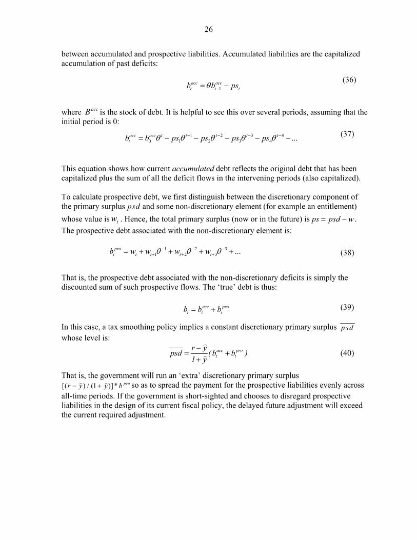
26
between accumulated and prospective liabilities. Accumulated liabilities are the capitalized accumulation of past deficits: where accB is the stock of debt. It is helpful to see this over several periods, assuming that the initial period is 0: This equation shows how current accumulated debt reflects the original debt that has been capitalized plus the sum of all the deficit flows in the intervening periods (also capitalized). To calculate prospective debt, we first distinguish between the discretionary component of the primary surplus psd and some non-discretionary element (for example an entitlement)
whose value is tw . Hence, the total primary surplus (now or in the future) is ps psd w .
The prospective debt associated with the non-discretionary element is: That is, the prospective debt associated with the non-discretionary deficits is simply the discounted sum of such prospective flows. The ‘true’ debt is thus: In this case, a tax smoothing policy implies a constant discretionary primary surplus p sd
whose level is: That is, the government will run an ‘extra’ discretionary primary surplus[( ) / (1 )]* pror y y b so as to spread the payment for the prospective liabilities evenly across all-time periods. If the government is short-sighted and chooses to disregard prospective liabilities in the design of its current fiscal policy, the delayed future adjustment will exceed the current required adjustment.
1 2 31 2 3 ...pro
t t t t tb w w w w (38)
1acc acct t tb b ps
1 2 3 40 1 2 3 4 ...acc acc t t t t t
tb b ps ps ps ps
(36)
(37)
acc prot t
r ypsd ( b b )
1 y
(39)
(40)
acc prot t tb b b
27
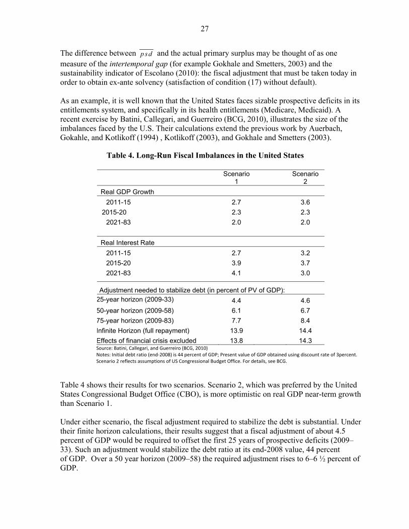
The difference between p sd and the actual primary surplus may be thought of as one measure of the intertemporal gap (for example Gokhale and Smetters, 2003) and the sustainability indicator of Escolano (2010): the fiscal adjustment that must be taken today in order to obtain ex-ante solvency (satisfaction of condition (17) without default). As an example, it is well known that the United States faces sizable prospective deficits in its entitlements system, and specifically in its health entitlements (Medicare, Medicaid). A recent exercise by Batini, Callegari, and Guerreiro (BCG, 2010), illustrates the size of the imbalances faced by the U.S. Their calculations extend the previous work by Auerbach, Gokahle, and Kotlikoff (1994) , Kotlikoff (2003), and Gokhale and Smetters (2003).
Scenario
1 Scenario
2
Real GDP Growth
2011-15 2.7 3.6
2015-20 2.3 2.3
2021-83 2.0 2.0
Real Interest Rate
2011-15 2.7 3.2
2015-20 3.9 3.7
2021-83 4.1 3.0
Adjustment needed to stabilize debt (in percent of PV of GDP):25-year horizon (2009-33) 4.4 4.6
50-year horizon (2009-58) 6.1 6.7
75-year horizon (2009-83) 7.7 8.4
Infinite Horizon (full repayment) 13.9 14.4
Effects of financial crisis excluded 13.8 14.3 Source: Batini, Callegari, and Guerreiro (BCG, 2010) Notes: Initial debt ratio (end-2008) is 44 percent of GDP; Present value of GDP obtained using discount rate of 3percent. Scenario 2 reflects assumptions of US Congressional Budget Office. For details, see BCG.
Table 4 shows their results for two scenarios. Scenario 2, which was preferred by the United States Congressional Budget Office (CBO), is more optimistic on real GDP near-term growth than Scenario 1. Under either scenario, the fiscal adjustment required to stabilize the debt is substantial. Under their finite horizon calculations, their results suggest that a fiscal adjustment of about 4.5 percent of GDP would be required to offset the first 25 years of prospective deficits (2009–33). Such an adjustment would stabilize the debt ratio at its end-2008 value, 44 percent of GDP. Over a 50 year horizon (2009–58) the required adjustment rises to 6–6 ½ percent of GDP.
Table 4. Long-Run Fiscal Imbalances in the United States
28
To offset the first 75 years (2009–83), the government would need to raise the primary surplus by about 8 percent. And, for an infinite horizon—to fully satisfy the no-Ponzi game condition—the required adjustment is around 14 percent of GDP. BCG also estimates that the effect of the financial crisis on prospective debt is small—about 0.1 percent of GDP.
IX. THE NET WORTH APPROACH
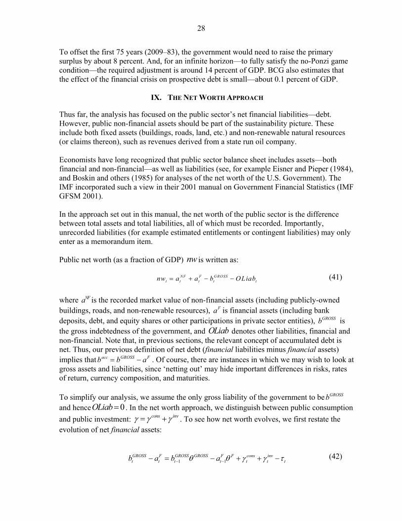
Thus far, the analysis has focused on the public sector’s net financial liabilities—debt. However, public non-financial assets should be part of the sustainability picture. These include both fixed assets (buildings, roads, land, etc.) and non-renewable natural resources (or claims thereon), such as revenues derived from a state run oil company. Economists have long recognized that public sector balance sheet includes assets—both financial and non-financial—as well as liabilities (see, for example Eisner and Pieper (1984), and Boskin and others (1985) for analyses of the net worth of the U.S. Government). The IMF incorporated such a view in their 2001 manual on Government Financial Statistics (IMF GFSM 2001). In the approach set out in this manual, the net worth of the public sector is the difference between total assets and total liabilities, all of which must be recorded. Importantly, unrecorded liabilities (for example estimated entitlements or contingent liabilities) may only enter as a memorandum item. Public net worth (as a fraction of GDP) nw is written as: NF F GROSS
t t t t tnw a a b OLiab
where NFa is the recorded market value of non-financial assets (including publicly-owned buildings, roads, and non-renewable resources), Fa is financial assets (including bank deposits, debt, and equity shares or other participations in private sector entities), GROSSb is the gross indebtedness of the government, and OLiab denotes other liabilities, financial and non-financial. Note that, in previous sections, the relevant concept of accumulated debt is net. Thus, our previous definition of net debt (financial liabilities minus financial assets) implies that acc GROSS Fb b a . Of course, there are instances in which we may wish to look at gross assets and liabilities, since ‘netting out’ may hide important differences in risks, rates of return, currency composition, and maturities. To simplify our analysis, we assume the only gross liability of the government to be GROSSb and hence 0OLiab . In the net worth approach, we distinguish between public consumption
and public investment: cons inv . To see how net worth evolves, we first restate the evolution of net financial assets:
1 1GROSS F GROSS GROSS F F cons invt t t t t t tb a b a
(41)
(42)
29
Next, note that non-financial assets earn a real rate of return net of depreciation equal to NF ; the gross return factor on non-financial assets, adjusted for real GDP growth is
(1 ) / (1 )NF NF y . Non financial assets hence evolve according to1
NF NF NF invt t ta a .
Thus, net worth (relative to GDP) evolves according to:
1 1 1NF NF F F GROSS GROSS cons
t t t t t tnw a a b
If the government seeks to service gross debt without a fiscal adjustment (raising tax rates or cutting spending), its gross financial assets may be liquidated. By contrast, non-financial assets that correspond to future (imputed) consumption do not provide such an option for debt service. To see this, consider a fully occupied public office building whose market value
tBUILD is equal to the present value of (imputed) rental payments for that building:
2 3
1 2 3/ (1 ) / (1 ) / (1 ) .... t t t t tBUILD RENT RENT r RENT r RENT r
The government may hypothetically sell that building and use its cash receipt tBUILD to
pay down the debt. But then the government must decide whether it will continue to use the office space provided by an equivalent building. If so, explicit rental flows will be reflected
in government consumption cons . Otherwise, a fiscal adjustment has effectively taken place.
X. NON-RENEWABLE RESOURCES
Some governments depend on funding from revenues derived from non-renewable natural resources (oil, mineral). Such governments must decide when these resources should be spent. Will future generations benefit from a country’s natural endowments? Or, will current governments prematurely deplete these resources? The ‘permanent income’ or ‘permanent consumption’ approach to this issue (see Barnett and Ossowski, 2003, Balassone, Takizawa, Zebregs, 2006, and others) can be easily integrated with other ideas presented in this paper. Under this approach the government treats a publicly-owned natural resource as if it were an asset that yields a flow of income that is available for public consumption – while also leaving the initial stock of assets intact. Under such an approach, the stock value of the natural resource must be estimated. As a simple example, assume that there is some exogenously determined optimal rate of extraction. Hence, in any period t, the oil company is expected to generate a surplus of tz .
This number is essentially the operational surplus of the oil company: it takes into account the market price of oil, the technical costs of extraction, and the wages paid to employees of the oil company. The oil wealth (ow) variable is at the end of period 0 (prior to any extraction) is defined as the present value of net oil revenues from period 1 until the depletion date N:
(43)
(44)
0
1
/
N
tt
t
ow z (45)
30
We also assume that there is a hypothetical financial asset called an oil fund (of). In this model, tof serves only as an accounting tool.30 The oil fund evolves according to:
1t tof of
Jointly, equations (45) and (46) have an intuitive interpretation. Prospective oil surpluses in any period zt are the incremental additions to the interest bearing oil fund. Oil in the ground is converted into an interest bearing financial that builds up over time. Our narrow measure of public net worth nnw is thus:31 t t t tnnw ow of b
This resource-based fund will generate interest payments. Note also that, since owt = owt-1 – zt, 1 t t tof of z and 1 t t tb b psno where psno is the non-oil primary surplus, we have
1 t t tnnw nnw psno
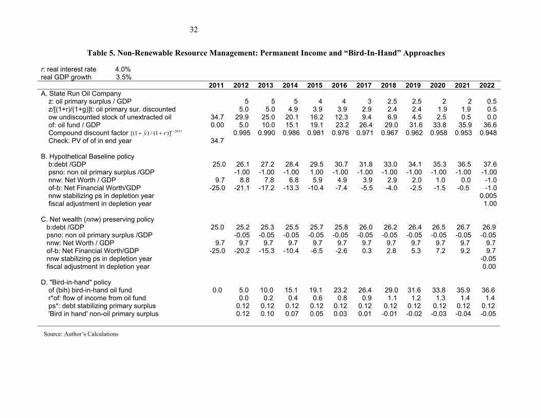
We may now obtain the non-oil primary surplus that stabilizes net worth *psno in a manner consistent with a permanent income approach If the government is a net creditor ( 0nnw ), it may run a non-oil primary deficit; if it is a net debtor ( 0nnw ), it must run a non-oil primary surplus. In this case, it is assumed that the government is able to borrow against future oil earnings and hence, smooth expenditures (taking advantage of credibility in capital markets). An example of the approach is presented in Table 5. A hypothetical country is assumed to grow by 3.5 percent and the interest rate (r) is 4 percent. In the initial period, t = 0, contributions to the oil fund have not yet begun. In this case, of0=0. In Part A of the table, the country’s public oil company is forecast to generate a series of net revenues (relative to GDP) from 2012 through 2022. The total value of oil wealth that is yet to be extracted ow0 is
30 A recent review of institutional arrangements designed to preserve natural resource wealth is Davis, Ossowski, and Fedelino eds., 2003. Also, Da Costa and Juan-Ramón (2006) highlight the distinction between an oil fund (that grows continually) and an oil stabilization fund (which might fluctuate about a constant mean). Here we do not address the question of who manages the oil fund. This can be critical: in some countries, the fund is managed by an agency that is independent from the day-to-day finances of the government. Such independence may be critical for achieving long-run fiscal sustainability.
31 For simplicity, this narrow measure of net worth does not include fixed capital (buildings, roads, etc).
(47)
(48)
(46)
t
r ypsno* nnw
1 y
(49)
31
estimated from 2011 to be 34.7 percent of GDP (based on prospective discounted revenues and costs). Oil revenues will be accumulated into an (accounting) oil fund whose initial value in 2011 is zero. Initial debt is 25 percent of GDP. Therefore, in 2011, this narrow measure of the country’s net worth 0 0 0( )nnw ow b is 9.7 percent of GDP.
The rate of return on the oil fund is identical to that paid on its debt—4 percent.32 Thus, the capitalized value of all oil proceeds in the year 2022—that is, the terminal value of the oil fund 2022of is 36.6 percent of GDP—a number whose present value equals oil wealth in the
initial period (34.7 percent of GDP). Part B of the table shows a baseline scenario in which the net worth measure nnw falls. The country runs a non-oil primary deficit of 1 percent of GDP ( 1%tpsno ). Under this
scenario, debt-GDP ratio rises from 25 percent to 37.6 percent of GDP in 2022. At the same time, the oil fund is increasing. Hence, by 2022, the net financial worth of the government, measured by t tof b has risen: in the initial period (2011), net financial worth is simply
minus unity times the debt— 2011 2011 25%of b . By the end period (2022), this number is
still negative, but less so, 2011 2011 1%.of b
It is easily seen how focusing exclusively on financial wealth can fundamentally distort the true picture of the public sector’s position. Beginning in 2022, if the government wishes to stabilize its net financial wealth position at -1 percent, it will have to make an adjustment to the non-oil primary surplus, since oil revenues will have ceased. From 2013 forward, the government will have to run a small non-oil primary surplus: 0.005%psno . This represents however an adjustment of just over 1 percent of GDP relative to the non-oil primary deficit that it had previously been running.
32 This critical assumption is relaxed below.
32
Table 5. Non-Renewable Resource Management: Permanent Income and “Bird-In-Hand” Approaches
r: real interest rate 4.0% real GDP growth 3.5%
2011 2012 2013 2014 2015 2016 2017 2018 2019 2020 2021 2022 A. State Run Oil Company z: oil primary surplus / GDP 5 5 5 4 4 3 2.5 2.5 2 2 0.5 z/[(1+r)/(1+g)]t: oil primary sur. discounted 5.0 5.0 4.9 3.9 3.9 2.9 2.4 2.4 1.9 1.9 0.5 ow undiscounted stock of unextracted oil 34.7 29.9 25.0 20.1 16.2 12.3 9.4 6.9 4.5 2.5 0.5 0.0 of: oil fund / GDP 0.00 5.0 10.0 15.1 19.1 23.2 26.4 29.0 31.6 33.8 35.9 36.6 Compound discount factor 0.995 0.990 0.986 0.981 0.976 0.971 0.967 0.962 0.958 0.953 0.948 Check: PV of of in end year 34.7
B. Hypothetical Baseline policy b:debt /GDP 25.0 26.1 27.2 28.4 29.5 30.7 31.8 33.0 34.1 35.3 36.5 37.6 psno: non oil primary surplus /GDP -1.00 -1.00 -1.00 1.00 -1.00 -1.00 -1.00 -1.00 -1.00 -1.00 -1.00 nnw: Net Worth / GDP 9.7 8.8 7.8 6.8 5.9 4.9 3.9 2.9 2.0 1.0 0.0 -1.0 of-b: Net Financial Worth/GDP -25.0 -21.1 -17.2 -13.3 -10.4 -7.4 -5.5 -4.0 -2.5 -1.5 -0.5 -1.0 nnw stabilizing ps in depletion year 0.005 fiscal adjustment in depletion year 1.00
C. Net wealth (nnw) preserving policy b:debt /GDP 25.0 25.2 25.3 25.5 25.7 25.8 26.0 26.2 26.4 26.5 26.7 26.9 psno: non oil primary surplus /GDP -0.05 -0.05 -0.05 -0.05 -0.05 -0.05 -0.05 -0.05 -0.05 -0.05 -0.05 nnw: Net Worth / GDP 9.7 9.7 9.7 9.7 9.7 9.7 9.7 9.7 9.7 9.7 9.7 9.7 of-b: Net Financial Worth/GDP -25.0 -20.2 -15.3 -10.4 -6.5 -2.6 0.3 2.8 5.3 7.2 9.2 9.7 nnw stabilizing ps in depletion year -0.05 fiscal adjustment in depletion year 0.00
D. "Bird-in-hand" policy of (bih) bird-in-hand oil fund 0.0 5.0 10.0 15.1 19.1 23.2 26.4 29.0 31.6 33.8 35.9 36.6 r*of: flow of income from oil fund 0.0 0.2 0.4 0.6 0.8 0.9 1.1 1.2 1.3 1.4 1.4 ps*: debt stabilizing primary surplus 0.12 0.12 0.12 0.12 0.12 0.12 0.12 0.12 0.12 0.12 0.12 'Bird in hand' non-oil primary surplus 0.12 0.10 0.07 0.05 0.03 0.01 -0.01 -0.02 -0.03 -0.04 -0.05 Source: Author’s Calculations
2011ˆ[(1 ) / (1 )]ty r

33
Part B shows that such an adjustment in 2013 can be avoided if the government instead aims to stabilize narrow net worth (nnw). Since narrow net worth is positive, the government can run a non-oil primary deficit, but that deficit must be smaller than the 1 percent it was running in the baseline scenario. Instead, we compute the net worth stabilizing value for the non-oil primary surplus to be: (.04 .035) / 1.035 * 9.7 0.05%psno -- about 1/20th of GDP. In choosing this smaller primary surplus, the government has effectively preserved a portion of the oil proceeds for consumption in the years 2013 and beyond. We can see that, under this policy, the government has ‘pre-stabilized’ its financial net worth for 2013 and afterwards. The adjustment of 1 percent in that year that was required to preserve net financial wealth is no longer necessary. Uncertainty presents challenges to the ‘permanent income’ approach. For example, it may be difficult to estimate the stock of commodity (oil) wealth, since commodity (oil) prices—in addition to economic growth and interest rates—are difficult to predict. An alternative proposed by some (see Barnett and Ossowski, 2002, Bjerkholdt, 2002, Balassone, Takizawa, Zebregs, 2006, and others) would count only the resources that have already been placed into the natural resource fund—not the present value of resources prior to extraction. The income that is considered to be a part of the ‘permanent income’ that is made available for consumption is thus only the interest proceeds from that accumulated fund. This more conservative ‘Bird-In-Hand’ (BIH) approach does not permit the government to borrow against resources that are not yet extracted. While there are a number of ways to implement a BIH rule, one way to do so would be to keep the debt constant. Under such a BIH approach, the non-oil primary surplus would evolve according to: The result of such a policy is shown in Part D of the table. Initially, when the oil fund is low, the government must run non-oil primary surpluses. As the oil fund accumulates, and more interest income from the oil fund becomes available, the primary surplus BIH
tpsno falls. In period N+1,
after the resource is depleted, the public sector can run a higher primary deficit than it would under the narrow net worth stabilizing policy, since it did not borrow from resources in the
ground under the former. That is, after resource depletion, *BIHpsno psno – but only slightly so. Uncertainty in world commodity prices suggests other modifications of the ‘permanent income’ approach to the management of natural resources. For resources whose depletion is projected to occur only in the distant future —a ‘large’ value of N—the authorities should make a ‘conservative’ estimate of the long-run commodity price (Barnett and Ossowski, 2003). The precautionary considerations discussed above in Section V would also carry over to natural resources: uncertainty in the long-run price of the export commodity is a reason for commodity exporters to run a structural surplus. For example, in an initial period, the authority might run a non-oil primary surplus that exceeds the stabilizing value *
0psno psno . If psno may also be
linked to asset accumulation, in a way that is similar to (30):
BIHt t t
r ypsno [ of b ]
1 y
(50)
SStt
r ypsno psno [ ]nnw
1 y
(51)
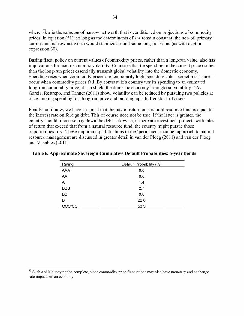
34
where nnw is the estimate of narrow net worth that is conditioned on projections of commodity prices. In equation (51), so long as the determinants of ow remain constant, the non-oil primary surplus and narrow net worth would stabilize around some long-run value (as with debt in expression 30). Basing fiscal policy on current values of commodity prices, rather than a long-run value, also has implications for macroeconomic volatility. Countries that tie spending to the current price (rather than the long-run price) essentially transmit global volatility into the domestic economy. Spending rises when commodity prices are temporarily high; spending cuts—sometimes sharp—occur when commodity prices fall. By contrast, if a country ties its spending to an estimated long-run commodity price, it can shield the domestic economy from global volatility.33 As Garcia, Restrepo, and Tanner (2011) show, volatility can be reduced by pursuing two policies at once: linking spending to a long-run price and building up a buffer stock of assets. Finally, until now, we have assumed that the rate of return on a natural resource fund is equal to the interest rate on foreign debt. This of course need not be true. If the latter is greater, the country should of course pay down the debt. Likewise, if there are investment projects with rates of return that exceed that from a natural resource fund, the country might pursue those opportunities first. These important qualifications to the ‘permanent income’ approach to natural resource management are discussed in greater detail in van der Ploeg (2011) and van der Ploeg and Venables (2011).
33 Such a shield may not be complete, since commodity price fluctuations may also have monetary and exchange rate impacts on an economy.
Rating Default Probability (%) AAA 0.0
AA 0.6
A 1.4
BBB 2.7
BB 9.0
B 22.0
CCC/CC 53.3
Table 6. Approximate Sovereign Cumulative Default Probabilities: 5-year bonds
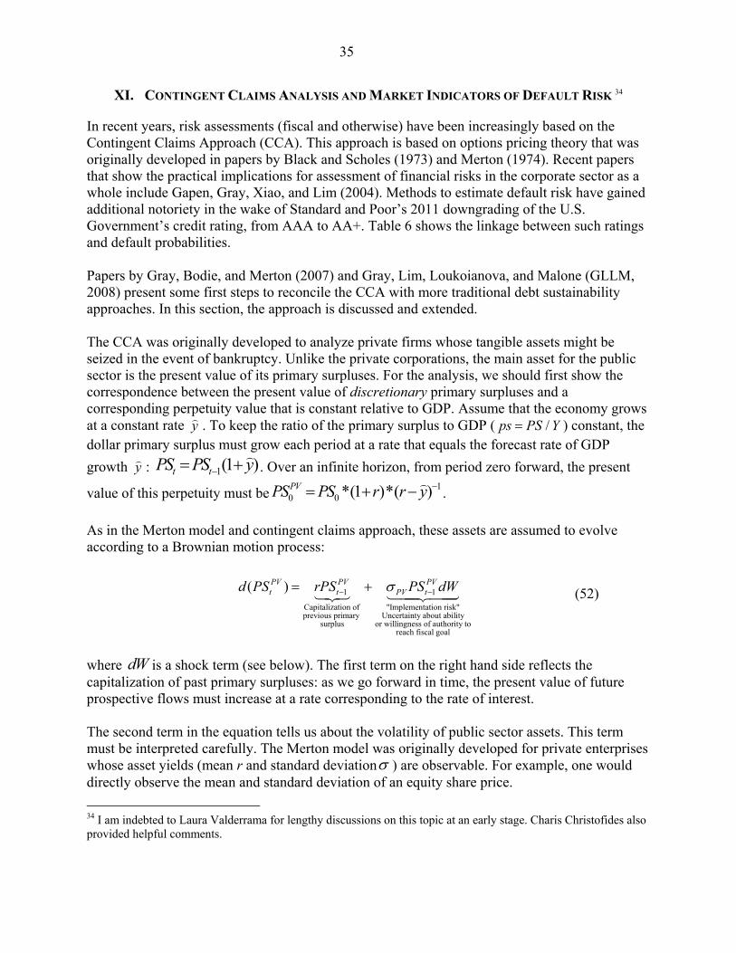
35
XI. CONTINGENT CLAIMS ANALYSIS AND MARKET INDICATORS OF DEFAULT RISK 34
In recent years, risk assessments (fiscal and otherwise) have been increasingly based on the Contingent Claims Approach (CCA). This approach is based on options pricing theory that was originally developed in papers by Black and Scholes (1973) and Merton (1974). Recent papers that show the practical implications for assessment of financial risks in the corporate sector as a whole include Gapen, Gray, Xiao, and Lim (2004). Methods to estimate default risk have gained additional notoriety in the wake of Standard and Poor’s 2011 downgrading of the U.S. Government’s credit rating, from AAA to AA+. Table 6 shows the linkage between such ratings and default probabilities. Papers by Gray, Bodie, and Merton (2007) and Gray, Lim, Loukoianova, and Malone (GLLM, 2008) present some first steps to reconcile the CCA with more traditional debt sustainability approaches. In this section, the approach is discussed and extended. The CCA was originally developed to analyze private firms whose tangible assets might be seized in the event of bankruptcy. Unlike the private corporations, the main asset for the public sector is the present value of its primary surpluses. For the analysis, we should first show the correspondence between the present value of discretionary primary surpluses and a corresponding perpetuity value that is constant relative to GDP. Assume that the economy grows at a constant rate y
. To keep the ratio of the primary surplus to GDP ( /ps PS Y ) constant, the
dollar primary surplus must grow each period at a rate that equals the forecast rate of GDP
growth y
: 1(1 )t tPS PS y . Over an infinite horizon, from period zero forward, the present
value of this perpetuity must be1
0 0 *(1 )*( )PVPS PS r r y .
As in the Merton model and contingent claims approach, these assets are assumed to evolve according to a Brownian motion process: where dW is a shock term (see below). The first term on the right hand side reflects the capitalization of past primary surpluses: as we go forward in time, the present value of future prospective flows must increase at a rate corresponding to the rate of interest. The second term in the equation tells us about the volatility of public sector assets. This term must be interpreted carefully. The Merton model was originally developed for private enterprises whose asset yields (mean r and standard deviation ) are observable. For example, one would directly observe the mean and standard deviation of an equity share price.
34 I am indebted to Laura Valderrama for lengthy discussions on this topic at an early stage. Charis Christofides also provided helpful comments.
1 1
Capitalization of "Implementation risk"previous primary Uncertainty about ability
surplus or willingness of authority toreach fiscal goal
( )PV PV PVt t PV td PS rPS PS dW
(52)
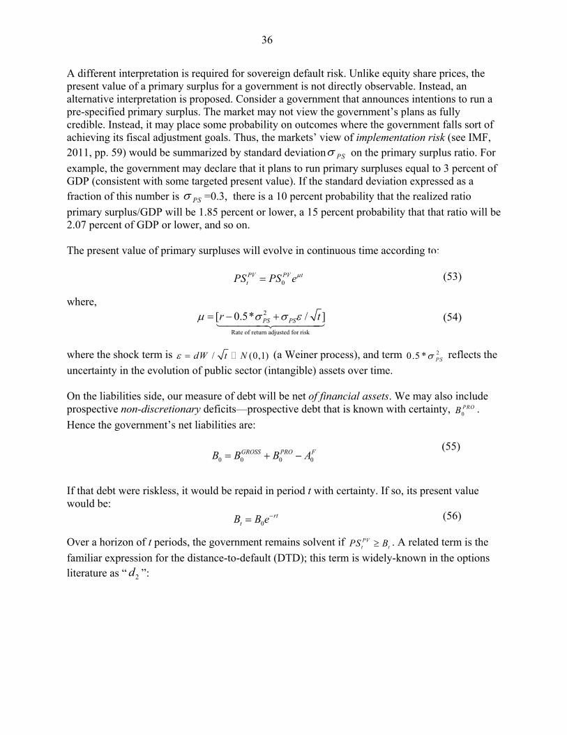
36
A different interpretation is required for sovereign default risk. Unlike equity share prices, the present value of a primary surplus for a government is not directly observable. Instead, an alternative interpretation is proposed. Consider a government that announces intentions to run a pre-specified primary surplus. The market may not view the government’s plans as fully credible. Instead, it may place some probability on outcomes where the government falls sort of achieving its fiscal adjustment goals. Thus, the markets’ view of implementation risk (see IMF, 2011, pp. 59) would be summarized by standard deviation PS on the primary surplus ratio. For
example, the government may declare that it plans to run primary surpluses equal to 3 percent of GDP (consistent with some targeted present value). If the standard deviation expressed as a fraction of this number is PS =0.3, there is a 10 percent probability that the realized ratio
primary surplus/GDP will be 1.85 percent or lower, a 15 percent probability that that ratio will be 2.07 percent of GDP or lower, and so on. The present value of primary surpluses will evolve in continuous time according to: where, where the shock term is / (0,1)dW t N (a Weiner process), and term 20.5 * PS reflects the
uncertainty in the evolution of public sector (intangible) assets over time. On the liabilities side, our measure of debt will be net of financial assets. We may also include prospective non-discretionary deficits—prospective debt that is known with certainty,
0PROB .
Hence the government’s net liabilities are:
If that debt were riskless, it would be repaid in period t with certainty. If so, its present value would be: Over a horizon of t periods, the government remains solvent if PV
t tPS B . A related term is the
familiar expression for the distance-to-default (DTD); this term is widely-known in the options literature as “ 2d ”:
0 0 0 0GROSS PRO FB B B A
0rt
tB B e
(55)
(56)
0PV PV ttPS PS e
2
Rate of return adjusted for risk
[ 0.5* / ]PS PSr t
(53)
(54)
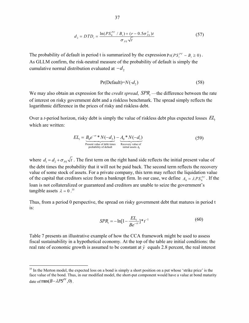
37
The probability of default in period t is summarized by the expression Pr( 0)PV
t tPS B .
As GLLM confirm, the risk-neutral measure of the probability of default is simply the cumulative normal distribution evaluated at 2d We may also obtain an expression for the credit spread, tSPR —the difference between the rate
of interest on risky government debt and a riskless benchmark. The spread simply reflects the logarithmic difference in the prices of risky and riskless debt. Over a t-period horizon, risky debt is simply the value of riskless debt plus expected losses tEL
which are written: where 1 2 PSd d t . The first term on the right hand side reflects the initial present value of
the debt times the probability that it will not be paid back. The second term reflects the recovery value of some stock of assets. For a private company, this term may reflect the liquidation value of the capital that creditors seize from a bankrupt firm. In our case, we define
0 0PVA PS . If the
loan is not collateralized or guaranteed and creditors are unable to seize the government’s tangible assets 0 .35 Thus, from a period 0 perspective, the spread on risky government debt that matures in period t is: Table 7 presents an illustrative example of how the CCA framework might be used to assess fiscal sustainability in a hypothetical economy. At the top of the table are initial conditions: the real rate of economic growth is assumed to be constant at y
equals 2.8 percent, the real interest
35 In the Merton model, the expected loss on a bond is simply a short position on a put whose ‘strike price’ is the face value of the bond. Thus, in our modified model, the short-put component would have a value at bond maturity
date of max( ,0)PVB PS .
20
2
ln( / ) ( 0.5 )PVt PS
t
PS
PS B r td DTD
t
0
0 2 0 1
Present value of debt times Recovery value of probability of default initial assets
* ( ) * ( )rtt
A
EL B e N d A N d
1ln[1 ]*tt rt
ELSPR t
Be
(57)
(59)
(60)
2Pr(Default)= (- )N d (58)
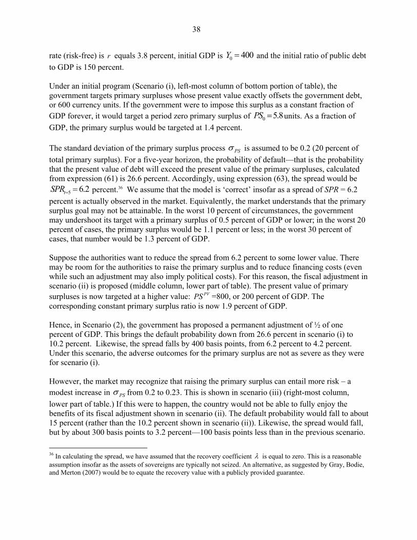
38
rate (risk-free) is r equals 3.8 percent, initial GDP is 0 400Y and the initial ratio of public debt
to GDP is 150 percent. Under an initial program (Scenario (i), left-most column of bottom portion of table), the government targets primary surpluses whose present value exactly offsets the government debt, or 600 currency units. If the government were to impose this surplus as a constant fraction of GDP forever, it would target a period zero primary surplus of 0 5.8PS units. As a fraction of
GDP, the primary surplus would be targeted at 1.4 percent. The standard deviation of the primary surplus process PS is assumed to be 0.2 (20 percent of
total primary surplus). For a five-year horizon, the probability of default—that is the probability that the present value of debt will exceed the present value of the primary surpluses, calculated from expression (61) is 26.6 percent. Accordingly, using expression (63), the spread would be
5 6.2tSPR percent.36 We assume that the model is ‘correct’ insofar as a spread of SPR = 6.2
percent is actually observed in the market. Equivalently, the market understands that the primary surplus goal may not be attainable. In the worst 10 percent of circumstances, the government may undershoot its target with a primary surplus of 0.5 percent of GDP or lower; in the worst 20 percent of cases, the primary surplus would be 1.1 percent or less; in the worst 30 percent of cases, that number would be 1.3 percent of GDP. Suppose the authorities want to reduce the spread from 6.2 percent to some lower value. There may be room for the authorities to raise the primary surplus and to reduce financing costs (even while such an adjustment may also imply political costs). For this reason, the fiscal adjustment in scenario (ii) is proposed (middle column, lower part of table). The present value of primary surpluses is now targeted at a higher value: PVPS =800, or 200 percent of GDP. The corresponding constant primary surplus ratio is now 1.9 percent of GDP. Hence, in Scenario (2), the government has proposed a permanent adjustment of ½ of one percent of GDP. This brings the default probability down from 26.6 percent in scenario (i) to 10.2 percent. Likewise, the spread falls by 400 basis points, from 6.2 percent to 4.2 percent. Under this scenario, the adverse outcomes for the primary surplus are not as severe as they were for scenario (i). However, the market may recognize that raising the primary surplus can entail more risk – a modest increase in PS from 0.2 to 0.23. This is shown in scenario (iii) (right-most column,
lower part of table.) If this were to happen, the country would not be able to fully enjoy the benefits of its fiscal adjustment shown in scenario (ii). The default probability would fall to about 15 percent (rather than the 10.2 percent shown in scenario (ii)). Likewise, the spread would fall, but by about 300 basis points to 3.2 percent—100 basis points less than in the previous scenario.
36 In calculating the spread, we have assumed that the recovery coefficient is equal to zero. This is a reasonable assumption insofar as the assets of sovereigns are typically not seized. An alternative, as suggested by Gray, Bodie, and Merton (2007) would be to equate the recovery value with a publicly provided guarantee.
39
This exercise has two main lessons. First, as is the case with any economic policy, the expectations surrounding a fiscal adjustment need to be well managed. If the authority proposes a fiscal adjustment, it should also take steps to make this adjustment credible. Otherwise, the government may not fully enjoy the gains to be had from lower financing costs (since PS has
risen). For this reason, fiscal adjustments should be clearly explained to the public. The second lesson regards the incentives for countries to adjust. An increase in the standard deviation PScan be seen as an implicit ‘tax’ on fiscal adjustment. This exercise thus suggests an alternative definition for maximum sustainable debt: the debt may be “too high” if a fiscal adjustment that also reduces the sovereign spread is not possible.
XII. SUMMARY AND CONCLUSIONS
This paper has attempted to integrate and comment on recent work in the area of fiscal sustainability. The issue was addressed from a positive point of view: What are the criteria for fiscal sustainability and are those criteria satisfied? This paper has attempted to integrate and comment on recent work in the area of fiscal sustainability. The issue was addressed from a positive point of view: What are the criteria for fiscal sustainability and are those criteria satisfied? In their assessment of fiscal policy in Fund programs, the Fund’s Independent Evaluation Office (IMF-IEO, 2003) noted that adjustment programs that included a fiscal component often failed to include an explicit forward-looking analysis of debt sustainability. Since that report was written, considerable progress has been made regarding positive sustainability assessments. The Fund’s DSA template was introduced at the time of the report; it continues to be presented in most country staff reports, with ongoing refinements. Beyond operational work, this paper has attempted to spotlight some of the recent efforts to develop and refine our methods for assessing fiscal sustainability under various forms of uncertainty. As a result of this work, our toolbox now contains more and better tools for positive assessments of debt sustainability than it did a decade ago. We also explored the issue from a normative point of view: what policy (or policies) should be implemented to bring about fiscal sustainability—and why such policies will benefit a country’s citizens. Here again, owing to considerable analytical work in recent years, our toolbox has more and better tools. The ultimate goal of policy assessments—using either explicit welfare calculations from a general equilibrium model or from a less formal criterion—is to make a case for disciplined and credible fiscal policies to policy makers in a clear and compelling manner.37
37Arguably, this has happened in the monetary arena: a robust debate about policy objectives and rules has supported polices that have helped reduce inflation rates.

40
GDP Growth 2.8%
Risk free intere r 3.8%
GDP Y0 400
Currency % of GDP
Debt B 600 150.0
Scenario
Variance of PS 2(A) 0.04 0.04 0.05
Std. Dev of PS (A) 0.2 0.2 0.23
Currency % of GDP Currency % of GDP Currency % of GDP
Constant primary surplus 5.8 1.4 7.7 1.9 7.7 1.9
Present value of Pri Sur PSPV
600.0 150.0 800.0 200.0 800.0 200.0
Horizon = 5 years
Distance to Default DTD 0.63 1.27 1.04
Probability of default N(-DTD) 26.6% 10.2% 14.9%
Spread SPR 6.2% 2.2% 3.2%
Implementation Risk Currency % of GDP Currency % of GDP Currency % of GDP
Primary suprlus , 10% level 3.6 0.9 4.8 1.2 4.2 1.1
Primary suprlus , 20% level 4.3 1.1 5.8 1.4 5.3 1.3
Primary suprlus , 30% level 5.0 1.3 6.7 1.7 6.2 1.6
Horizon = 10 years
Distance to Default DTD 0.9 0.9 1.1
Probability of default N(-DTD) 18.8% 18.8% 14.1%
Spread SPR 2.1% 2.1% 1.5%
Implementation Risk Currency % of GDP Currency % of GDP Currency % of GDP
Primary suprlus , 10% level 3.1 0.8 4.1 1.0 3.4 0.9
Primary suprlus , 20% level 4.1 1.0 5.4 1.4 4.7 1.2
Primary suprlus , 30% level 5.0 1.2 6.6 1.7 5.9 1.5
(i) Initial program (ii) Adjustment -no increase in
implementation risk
(iiI) Adjustment -increase in
implementation risk
PS
PSPSPS
PSPSPS
y
Table 7. Assessment of Fiscal Sustainability for a Hypothetical Economy: A Contingent Claims Approach
Source: Author’s Calculations

41
Also, while this paper has focused on how much fiscal adjustment is required for sustainability, other issues regarding the quality of fiscal policy must not be forgotten. These issues include reducing distortions and waste in a tax system and its administration, broadening the tax base, eliminating wasteful government expenditures, and providing public goods and services that achieve their goal in an efficient way. Such policies will support a broader policy goal: higher and more stable economic growth.
42
REFERENCES
Abel, Andrew B., N. Gregory Mankiw, Lawrence Summers, and Richard Zeckhauser, 1989, “Assessing Dynamic Efficiency: Theory and Evidence,” Review of Economic Studies, Vol. 56, No. 1 (January), pp 1–19.
Aiyagari, S. Rao, Albert Marcet, Thomas J. Sargent, and Juha Seppälä, 2002, “Optimal
Taxation without State-Contingent Debt,” Journal of Political Economy, Vol. 110, No. 6 (December), pp. 1220–54.
Alesina, Alberto and Guido Tabellini, 1990, “A Positive Theory of Fiscal Deficits and
Government Debt,” Review of Economic Studies, Vol. 57, No. 3 (July), pp. 403–14. Alesina, Alberto and Guido Tabellini, 1990, “Voting on the Budget Deficit,” American
Economic Review, Vol. 80, No. 1 (March), pp. 37–49. Altig, David, Alan J. Auerbach, Laurence J. Kotlikoff, Kent A. Smetters, and Jan Walliser,
2001, “Simulating Fundamental Tax Reform in the United States,” American Economic Review, Vol. 91, No. 3 (June), pp. 574–95.
Auerbach, Alan J., Jagddesh Gokhale, and Jagadeesh and Laurence Kotlikoff, 1994,
“Generational Accounting: A Meaningful Way to Evaluate Fiscal Policy,” Journal of Economic Perspectives, American Economic Association, Vol. 8, No. 1 (Winter), pp. 73–94.
Balassone, Fabrizio, Hajime Takizawa, and Harm Zebregs, 2006, “Russian Federation:
Selected Issues,” in IMF Staff Country Report No. 06/430, pp. 3–24 (Washington: International Monetary Fund). www.imf.org/external/pubs/ft/scr/2006/cr06430.pdf
Bandiera, Luca, Nina Budina, Michel Klijn, and Sweder Van Wijnbergen, 2007, “The 'How To' of Fiscal Sustainability: A Technical Manual for Using the Fiscal Sustainability Tool,” Policy Research Working Paper No. 4170 (Washington: World Bank).
Barnett, Steven and Rolando J. Ossowski, 2003, “Operational Aspects of Fiscal Policy in
Oil-Producing Countries,” in Fiscal Policy Formulation and Implementation in Oil- Producing Countries, edited by Jeffrey M. Davis, Rolando J. Ossowski, and Annalisa Fedelino (Washington: International Monetary Fund).
Barro, Robert J., 1979, “On the Determination of the Public Debt,” Journal of Political
Economy, Vol. 87, No. 5 (October), pp. 940–71. Batini, Nicoletta, Giovanni Callegari, and Julia Guerreiro, 2010, “The US Fiscal Gap: Who
Will Pay and How?” in United States: Selected Issues Paper, IMF Country Report 10/248, pp. 52–67, http://www.imf.org/external/pubs/cat/longres.aspx?sk=24106.0.
43
Black, Fischer and Myron Scholes, 1973, “The Pricing of Options and Corporate Liabilities, ” Journal of Political Economy, Vol. 81, No. 3, pp. 637–54.
Blanchard, Olivier Jean and Stanley Fischer, 1989, Lectures On Macroeconomics
(Cambridge: MIT Press). Blanchard, Olivier Jean and Philippe Weil, 2001, “Dynamic Efficiency, the Riskless Rate,
and Debt Ponzi Games under Uncertainty,” The B.E. Journal of Macroeconomics, Vol. 1, Issue 2.
Bohn, Henning, 1998, “The Behavior of U.S. Public Debt and Deficits,” Quarterly Journal of Economics, Vol. 113, No. 3, pp. 949–63.
Bohn, H., 2008, “The Sustainability of Fiscal Policy in the United States,” in Sustainability
of Public Debt, ed. by Reinhard Neck and Jan-Egbert Sturm, pp. 15–49 (Cambridge, Massachusetts: MIT Press).
Boskin, Michael J., Marc S. Robinson, Terrence O'Reilly, and Praveen Kumar, 1985, “New
Estimates of the Value of Federal Mineral Rights and Land, ” American Economic Review, Vol. 75, No. 5 (December), pp. 923–36.
Budina, Nina and Sweder Van Wijnbergen, 2009, “Quantitative Approaches to Fiscal
Sustainability Analysis: A Case Study of Turkey Since the Crisis of 2001,” World Bank Economic Review, Vol. 23, No. 1, pp. 119–40.
Carroll, Christopher D. and Miles S. Kimball, 1996, “On the Concavity of the Consumption
Function,” Econometrica, Vol. 64, No. 4, (July), pp. 981–92. Caballero, Ricardo, 1990, “Consumption Puzzles and Precautionary Savings,” Journal of
Monetary Economics, Vol. 25, pp. 113–16. Celasun, O. X. Debrun and J. Ostry, 2007, “Primary Surplus Behavior and Risks to Fiscal
Sustainability in Emerging Market Countries: A “Fan-Chart” Approach,” Staff Papers, International Monetary Fund, Vol. 53, No. 3.
Chari, V., Lawrence J. Christiano and Patrick J. Kehoe, 1994, “Optimal Fiscal Policy in a
Business Cycle Model,” Journal of Political Economy, Vol. 102, No. 4, pp. 617–52. Cochrane, John, 1998, “A Frictionless View of U.S. Inflation,” in NBER Macroeconomics
Annual 1998, eds. Ben S. Bernanke and Julio Rotemberg, Vol.13 (Cambridge: Massachusetts, National Bureau of Economic Research).
Da Costa, Mercedes and V. Hugo Juan-Ramon, 2006, “The Net Worth Approach to Fiscal
Analysis: Dynamics and Rules,” IMF Working Paper 06/17 (Washington: International Monetay Fund). www.imf.org/external/pubs/ft/wp/2006/wp0617.pdf
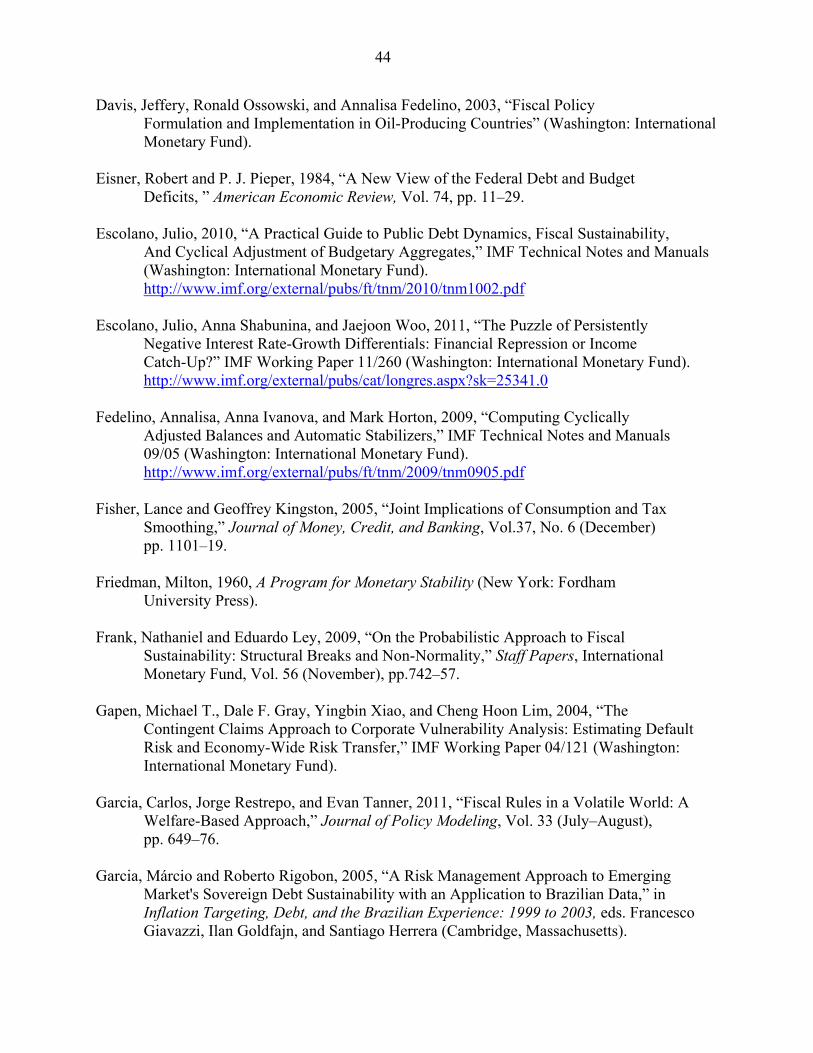
44
Davis, Jeffery, Ronald Ossowski, and Annalisa Fedelino, 2003, “Fiscal Policy Formulation and Implementation in Oil-Producing Countries” (Washington: International Monetary Fund).
Eisner, Robert and P. J. Pieper, 1984, “A New View of the Federal Debt and Budget
Deficits, ” American Economic Review, Vol. 74, pp. 11–29. Escolano, Julio, 2010, “A Practical Guide to Public Debt Dynamics, Fiscal Sustainability,
And Cyclical Adjustment of Budgetary Aggregates,” IMF Technical Notes and Manuals (Washington: International Monetary Fund). http://www.imf.org/external/pubs/ft/tnm/2010/tnm1002.pdf
Escolano, Julio, Anna Shabunina, and Jaejoon Woo, 2011, “The Puzzle of Persistently
Negative Interest Rate-Growth Differentials: Financial Repression or Income Catch-Up?” IMF Working Paper 11/260 (Washington: International Monetary Fund). http://www.imf.org/external/pubs/cat/longres.aspx?sk=25341.0
Fedelino, Annalisa, Anna Ivanova, and Mark Horton, 2009, “Computing Cyclically
Adjusted Balances and Automatic Stabilizers,” IMF Technical Notes and Manuals 09/05 (Washington: International Monetary Fund). http://www.imf.org/external/pubs/ft/tnm/2009/tnm0905.pdf
Fisher, Lance and Geoffrey Kingston, 2005, “Joint Implications of Consumption and Tax
Smoothing,” Journal of Money, Credit, and Banking, Vol.37, No. 6 (December) pp. 1101–19.
Friedman, Milton, 1960, A Program for Monetary Stability (New York: Fordham
University Press). Frank, Nathaniel and Eduardo Ley, 2009, “On the Probabilistic Approach to Fiscal
Sustainability: Structural Breaks and Non-Normality,” Staff Papers, International Monetary Fund, Vol. 56 (November), pp.742–57.
Gapen, Michael T., Dale F. Gray, Yingbin Xiao, and Cheng Hoon Lim, 2004, “The
Contingent Claims Approach to Corporate Vulnerability Analysis: Estimating Default Risk and Economy-Wide Risk Transfer,” IMF Working Paper 04/121 (Washington: International Monetary Fund).
Garcia, Carlos, Jorge Restrepo, and Evan Tanner, 2011, “Fiscal Rules in a Volatile World: A
Welfare-Based Approach,” Journal of Policy Modeling, Vol. 33 (July–August), pp. 649–76.
Garcia, Márcio and Roberto Rigobon, 2005, “A Risk Management Approach to Emerging
Market's Sovereign Debt Sustainability with an Application to Brazilian Data,” in Inflation Targeting, Debt, and the Brazilian Experience: 1999 to 2003, eds. Francesco Giavazzi, Ilan Goldfajn, and Santiago Herrera (Cambridge, Massachusetts).
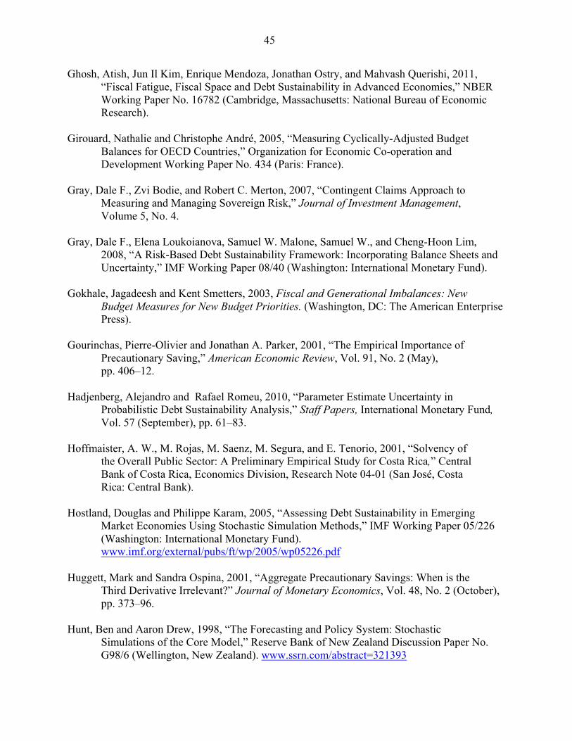
45
Ghosh, Atish, Jun Il Kim, Enrique Mendoza, Jonathan Ostry, and Mahvash Querishi, 2011, “Fiscal Fatigue, Fiscal Space and Debt Sustainability in Advanced Economies,” NBER Working Paper No. 16782 (Cambridge, Massachusetts: National Bureau of Economic Research).
Girouard, Nathalie and Christophe André, 2005, “Measuring Cyclically-Adjusted Budget
Balances for OECD Countries,” Organization for Economic Co-operation and Development Working Paper No. 434 (Paris: France).
Gray, Dale F., Zvi Bodie, and Robert C. Merton, 2007, “Contingent Claims Approach to
Measuring and Managing Sovereign Risk,” Journal of Investment Management, Volume 5, No. 4.
Gray, Dale F., Elena Loukoianova, Samuel W. Malone, Samuel W., and Cheng-Hoon Lim,
2008, “A Risk-Based Debt Sustainability Framework: Incorporating Balance Sheets and Uncertainty,” IMF Working Paper 08/40 (Washington: International Monetary Fund).
Gokhale, Jagadeesh and Kent Smetters, 2003, Fiscal and Generational Imbalances: New
Budget Measures for New Budget Priorities. (Washington, DC: The American Enterprise Press).
Gourinchas, Pierre-Olivier and Jonathan A. Parker, 2001, “The Empirical Importance of
Precautionary Saving,” American Economic Review, Vol. 91, No. 2 (May), pp. 406–12.
Hadjenberg, Alejandro and Rafael Romeu, 2010, “Parameter Estimate Uncertainty in
Probabilistic Debt Sustainability Analysis,” Staff Papers, International Monetary Fund, Vol. 57 (September), pp. 61–83.
Hoffmaister, A. W., M. Rojas, M. Saenz, M. Segura, and E. Tenorio, 2001, “Solvency of
the Overall Public Sector: A Preliminary Empirical Study for Costa Rica,” Central Bank of Costa Rica, Economics Division, Research Note 04-01 (San José, Costa Rica: Central Bank).
Hostland, Douglas and Philippe Karam, 2005, “Assessing Debt Sustainability in Emerging
Market Economies Using Stochastic Simulation Methods,” IMF Working Paper 05/226 (Washington: International Monetary Fund). www.imf.org/external/pubs/ft/wp/2005/wp05226.pdf
Huggett, Mark and Sandra Ospina, 2001, “Aggregate Precautionary Savings: When is the
Third Derivative Irrelevant?” Journal of Monetary Economics, Vol. 48, No. 2 (October), pp. 373–96.
Hunt, Ben and Aaron Drew, 1998, “The Forecasting and Policy System: Stochastic Simulations of the Core Model,” Reserve Bank of New Zealand Discussion Paper No. G98/6 (Wellington, New Zealand). www.ssrn.com/abstract=321393
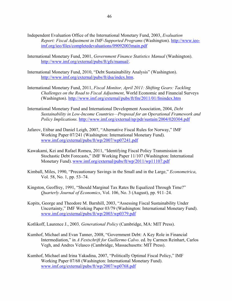
46
Independent Evaluation Office of the International Monetary Fund, 2003, Evaluation
Report: Fiscal Adjustment in IMF-Supported Programs (Washington). http://www.ieo-imf.org/ieo/files/completedevaluations/09092003main.pdf
International Monetary Fund, 2001, Government Finance Statistics Manual (Washington). http://www.imf.org/external/pubs/ft/gfs/manual/.
International Monetary Fund, 2010, “Debt Sustainability Analysis” (Washington). http://www.imf.org/external/pubs/ft/dsa/index.htm.
International Monetary Fund, 2011, Fiscal Monitor, April 2011: Shifting Gears: Tackling Challenges on the Road to Fiscal Adjustment, World Economic and Financial Surveys (Washington). http://www.imf.org/external/pubs/ft/fm/2011/01/fmindex.htm
International Monetary Fund and International Development Association, 2004, Debt Sustainability in Low-Income Countries—Proposal for an Operational Framework and Policy Implications. http://www.imf.org/external/np/pdr/sustain/2004/020304.pdf
Jafarov, Etibar and Daniel Leigh, 2007, “Alternative Fiscal Rules for Norway,” IMF
Working Paper 07/241 (Washington: International Monetary Fund).
www.imf.org/external/pubs/ft/wp/2007/wp07241.pdf Kawakami, Kei and Rafael Romeu, 2011, “Identifying Fiscal Policy Transmission in
Stochastic Debt Forecasts,” IMF Working Paper 11/107 (Washington: International Monetary Fund). www.imf.org/external/pubs/ft/wp/2011/wp11107.pdf
Kimball, Miles, 1990, “Precautionary Savings in the Small and in the Large,” Econometrica, Vol. 58, No. 1, pp. 53–74.
Kingston, Geoffrey, 1991, “Should Marginal Tax Rates Be Equalized Through Time?”
Quarterly Journal of Economics, Vol. 106, No. 3 (August), pp. 911–24. Kopits, George and Theodore M. Barnhill, 2003, “Assessing Fiscal Sustainability Under
Uncertainty,” IMF Working Paper 03/79 (Washington: International Monetary Fund). www.imf.org/external/pubs/ft/wp/2003/wp0379.pdf
Kotlikoff, Laurence J., 2003, Generational Policy (Cambridge, MA: MIT Press). Kumhof, Michael and Evan Tanner, 2008, “Government Debt: A Key Role in Financial
Intermediation,” in A Festschrift for Guillermo Calvo. ed. by Carmen Reinhart, Carlos Vegh, and Andres Velasco (Cambridge, Massachusetts: MIT Press).
Kumhof, Michael and Irina Yakadina, 2007, “Politically Optimal Fiscal Policy,” IMF
Working Paper 07/68 (Washington: International Monetary Fund).
www.imf.org/external/pubs/ft/wp/2007/wp0768.pdf
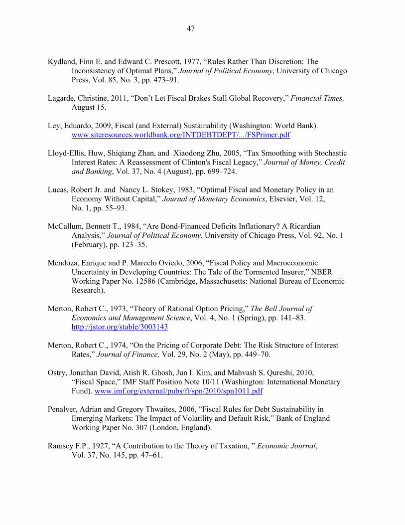
47
Kydland, Finn E. and Edward C. Prescott, 1977, “Rules Rather Than Discretion: The
Inconsistency of Optimal Plans,” Journal of Political Economy, University of Chicago Press, Vol. 85, No. 3, pp. 473–91.
Lagarde, Christine, 2011, “Don’t Let Fiscal Brakes Stall Global Recovery,” Financial Times,
August 15. Ley, Eduardo, 2009, Fiscal (and External) Sustainability (Washington: World Bank).
www.siteresources.worldbank.org/INTDEBTDEPT/.../FSPrimer.pdf Lloyd-Ellis, Huw, Shiqiang Zhan, and Xiaodong Zhu, 2005, “Tax Smoothing with Stochastic
Interest Rates: A Reassessment of Clinton's Fiscal Legacy,” Journal of Money, Credit and Banking, Vol. 37, No. 4 (August), pp. 699–724.
Lucas, Robert Jr. and Nancy L. Stokey, 1983, “Optimal Fiscal and Monetary Policy in an
Economy Without Capital,” Journal of Monetary Economics, Elsevier, Vol. 12, No. 1, pp. 55–93.
McCallum, Bennett T., 1984, “Are Bond-Financed Deficits Inflationary? A Ricardian
Analysis,” Journal of Political Economy, University of Chicago Press, Vol. 92, No. 1 (February), pp. 123–35.
Mendoza, Enrique and P. Marcelo Oviedo, 2006, “Fiscal Policy and Macroeconomic
Uncertainty in Developing Countries: The Tale of the Tormented Insurer,” NBER Working Paper No. 12586 (Cambridge, Massachusetts: National Bureau of Economic Research).
Merton, Robert C., 1973, “Theory of Rational Option Pricing,” The Bell Journal of
Economics and Management Science, Vol. 4, No. 1 (Spring), pp. 141–83. http://jstor.org/stable/3003143
Merton, Robert C., 1974, “On the Pricing of Corporate Debt: The Risk Structure of Interest
Rates,” Journal of Finance, Vol. 29, No. 2 (May), pp. 449–70. Ostry, Jonathan David, Atish R. Ghosh, Jun I. Kim, and Mahvash S. Qureshi, 2010,
“Fiscal Space,” IMF Staff Position Note 10/11 (Washington: International Monetary Fund). www.imf.org/external/pubs/ft/spn/2010/spn1011.pdf
Penalver, Adrian and Gregory Thwaites, 2006, “Fiscal Rules for Debt Sustainability in
Emerging Markets: The Impact of Volatility and Default Risk,” Bank of England Working Paper No. 307 (London, England).
Ramsey F.P., 1927, “A Contribution to the Theory of Taxation, ” Economic Journal,
Vol. 37, No. 145, pp. 47–61.
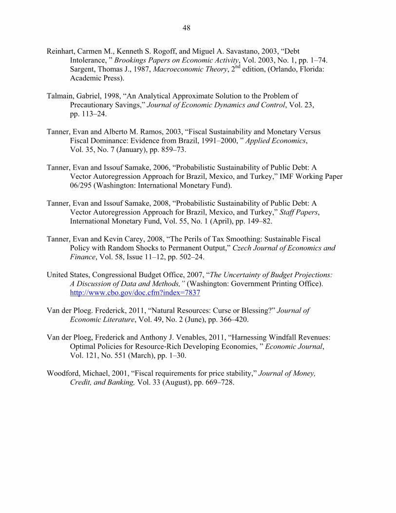
48
Reinhart, Carmen M., Kenneth S. Rogoff, and Miguel A. Savastano, 2003, “Debt Intolerance, ” Brookings Papers on Economic Activity, Vol. 2003, No. 1, pp. 1–74. Sargent, Thomas J., 1987, Macroeconomic Theory, 2nd edition, (Orlando, Florida: Academic Press).
Talmain, Gabriel, 1998, “An Analytical Approximate Solution to the Problem of
Precautionary Savings,” Journal of Economic Dynamics and Control, Vol. 23, pp. 113–24.
Tanner, Evan and Alberto M. Ramos, 2003, “Fiscal Sustainability and Monetary Versus
Fiscal Dominance: Evidence from Brazil, 1991–2000, ” Applied Economics, Vol. 35, No. 7 (January), pp. 859–73.
Tanner, Evan and Issouf Samake, 2006, “Probabilistic Sustainability of Public Debt: A
Vector Autoregression Approach for Brazil, Mexico, and Turkey,” IMF Working Paper 06/295 (Washington: International Monetary Fund).
Tanner, Evan and Issouf Samake, 2008, “Probabilistic Sustainability of Public Debt: A
Vector Autoregression Approach for Brazil, Mexico, and Turkey,” Staff Papers, International Monetary Fund, Vol. 55, No. 1 (April), pp. 149–82.
Tanner, Evan and Kevin Carey, 2008, “The Perils of Tax Smoothing: Sustainable Fiscal
Policy with Random Shocks to Permanent Output,” Czech Journal of Economics and Finance, Vol. 58, Issue 11–12, pp. 502–24.
United States, Congressional Budget Office, 2007, “The Uncertainty of Budget Projections:
A Discussion of Data and Methods,” (Washington: Government Printing Office). http://www.cbo.gov/doc.cfm?index=7837
Van der Ploeg. Frederick, 2011, “Natural Resources: Curse or Blessing?” Journal of
Economic Literature, Vol. 49, No. 2 (June), pp. 366–420. Van der Ploeg, Frederick and Anthony J. Venables, 2011, “Harnessing Windfall Revenues:
Optimal Policies for Resource‐Rich Developing Economies, ” Economic Journal, Vol. 121, No. 551 (March), pp. 1–30.
Woodford, Michael, 2001, “Fiscal requirements for price stability,” Journal of Money,
Credit, and Banking, Vol. 33 (August), pp. 669–728.