fiscal consolidations and heterogeneous expectations · fiscal consolidations and heterogeneous...
TRANSCRIPT
Fiscal Consolidations and Heterogeneous Expectations
Cars Hommes∗a,c, Joep Lustenhouwera,c and Kostas Mavromatisb
aCeNDEF, University of Amsterdam
bMInt, University of Amsterdam
cTinbergen Institute, Amsterdam
May 1, 2015
Abstract
We analyze fiscal consolidations using a New Keynesian model where agents have
heterogeneous expectations and are uncertain about the composition of consolidations.
Heterogeneity in expectations may amplify expansions, stabilizing thus the debt-to-GDP
ratio faster under tax based consolidations, in the short run. In the medium to long-run
though, the magnitude of the consolidation may favor spending cuts as long as agents
anticipate tax increases. Interestingly, wrong beliefs about the composition of fiscal con-
solidation may improve or harm the effectiveness of the latter, depending on the degree
of heterogeneity.
∗Email addresses: [email protected], [email protected], [email protected]
1 Introduction
The recent financial crisis gave rise to various types of government interventions. These inter-
ventions led to rising government debt levels in most advanced economies (see IMF (2011)).
Consequently, the majority of governments of those economies started the implementation of
consolidation policies. In the Eurozone, such policies are still pursued in an effort to over-
come a long lasting debt crisis in the countries of the Periphery. The debt crisis reshaped
the way governments within and outside the Monetary Union think in terms of fiscal policy.
In particular, the necessity for fiscal sustainability has arisen with the ultimate purpose of
enhancing growth.
In the literature, there is substantial evidence on the effects of fiscal consolidations. In
particular, there has been much research over the effects of different types of fiscal consol-
idations. That is, spending-based and tax-based consolidations. Moreover, the duration of
consolidations is of substantial importance. There is a number of empirical studies arguing
in favor of spending cuts as they tend to boost growth, contrary to tax increases (see Alesina
and Perotti (1995),Perotti (1996),Alesina and Ardagna (1998, 2010), Ardagna (2004)).
Following the recent empirical facts, on the theoretical side, the analysis of fiscal consoli-
dations has regained interest. Bi et al. (2013) construct a New Keynesian model and analyze
the effects of different types of fiscal consolidations. Moreover, they look at the effects of
persistence in those, as well as of uncertainty of economic agents over the type of the upcom-
ing fiscal consolidation. Accounting for the monetary policy stance as well, they find that
spending and tax-based consolidations can be equally successful in stabilizing government
debt at low debt levels. Nevertheless, at high debt levels, spending based consolidations are
expected to be expansionary and more successful in stabilizing debt, especially when agents
anticipate a tax-based consolidation.
The theoretical literature on consolidations, so far, has assumed that agents are fully
rational. The failure of traditional rational expectations models to capture some key facts in
the data, especially after the recent financial crisis, raised the need for a richer modeling of
economic behavior. In fact, there is very little evidence about the effects of fiscal consolidations
when agents are not behaving fully rational at all times. In this paper, we try to bridge this
gap by building a New Keynesian model with distortionary taxes where agents are boundedly
rational in the spirit of Brock and Hommes (1997). In particular, we assume that there are two
2
types of agents in the economy. Namely, the Fundamentalists and the Naive agents. The first
fraction uses policy (e.g. monetary and fiscal) announced rules when it forms its expectations
about inflation and output. In particular, Fundamentalists take into account the commitment
of the central bank to price stability. Moreover, when forming their expectations, they take
into account the commitment of fiscal authority to stabilize debt-to-GDP when the latter
exceeds a certain limit. On the contrary, Naive agents ignore the commitments of the two
authorities when forming their expectations. Hence, they naively use past information, only,
in order to predict inflation and output. Agents can switch between those two types according
a endogenous fitness measure. Agents choose the type with the higher fitness measure (i.e.
lower past forecast error).
Following Bi et al. (2013), we introduce uncertainty about the nature of fiscal consolida-
tions. In particular, agents are uncertain about whether consolidation will be tax-based or
spending-based once debt exceeds a known debt limit. As a result, they assign a probability
to the occurrence of each type of consolidation. Given that the fiscal authority implements
consolidations with a certain lag, this type of uncertainty affects expectations of fundamen-
talists. This is due to the assumption that those agents are forward looking and take into
account the future monetary/fiscal policy stance.
We find that tax-based consolidations lead to a quick drop in debt-to-GDP ratio in the
short-run, as opposed to spending based consolidations when fundamentalists anticipate the
latter. Interestingly, in the period before consolidation, output expands due to the expected
spending cuts. We show that, in this case, once the tax-based consolidation is implemented
fundamentalists realize that they were wrong when forming their expectations. This leads to
a rise in the fraction of naive agents the next period, which in turn leads to longer expansions
following the consolidation. On the contrary, when consolidation is spending-based, output
contracts abruptly upon consolidation and continues to contract throughout the consolidation.
Tax-based consolidations continue to be more successful in stabilizing debt in the short-
run, when fundamentalists believe that they are more likely to happen. We show that, in
this case, output contracts in the period before implementation. Once implemented, the
rise in distortionary taxes increases marginal costs and, hence, inflation. Since monetary
policy satisfies the Taylor principle, the rise in inflation leads to an increase in real interest
rates which intensifies the initial contraction in output. However, given that the debt ratio
3
falls faster below the debt limit under tax-based consolidations, the duration of consolidation
lasts less which stops output from contracting. In the medium to long-run, spending-based
consolidations might outperform tax-based, when the latter is anticipated, leading to lower a
debt ratio, as long as they have a high enough magnitude. This is achieved, though, at the
expense of a longer contraction in output. This is because it takes longer for the debt-to-GDP
to fall below the debt limit which raises the duration of consolidation.
Our findings contribute to the existing literature in many ways. To the best of our
knowledge, this is the first paper to analyze fiscal consolidations when agents are boundedly
rational. We distinguish between the short and long-run effects of fiscal consolidations in terms
of their performance in stabilizing debt. In line with the existing literature, we show that
the magnitude, the duration, the composition and the likelihood of consolidation matter in
determining the extend to which a specific type of consolidation is successful in stabilizing debt
and/or expansionary. Our major contribution, though, is that the assumption of boundedly
rational agents leads to much richer dynamics and policy implications that may differ to those
under rational expectations, substantially.
The next section outlines the model and the fiscal consolidations that may occur. Section 3
describes introduces heterogeneity in the way agents form expectations. Section 4 illustrates
the complete model after aggregation. Section 5 describes how effective the two types of
consolidations are under different private sector expectations. Section 6 concludes.
2 Model
2.1 Households
There is a continuum of households that differ in the way they form expectations. In par-
ticular, a household can be either naive or fundamentalist. Households of the same type
have the same preferences and make identical decisions. The intratemporal problem of each
household i, consists of choosing consumption over different goods to minimize expenditure.
This implies
Cit(j) =
(pt(j)
Pt
)−θCit , (1)
4
with Cit and Pt total consumption of the household and the aggregate price level, defined by
Cit =
(∫ 1
0Cit(j)
θ−1θ dj
) θθ−1
, (2)
Pt =
(∫ 1
0Pt(j)
1−θdj
) 11−θ
, (3)
where θ is the elasticity of substitution between the different goods.
Even though the horizon of the model is infinite, the households are short-sighted. That is,
they form expectations about one period ahead, only. The household i chooses consumption
(Cit), labor (H it), and nominal bond holdings (Bi
t). Hence, the maximization problem of the
household is summarized as
maxC,H,B
u(Cit , Hit) + βEitu(Cit+1, H
it+1), (4)
subject to its budget constraint
PtCit +Bi
t ≤ (1− τt)WtHit + (1− it−1)Bi
t−1 + Ξt, (5)
where Wt is the nominal wage, τt is the labor tax rate, and it is the nominal interest rate
and. Ξt represents profits received by firms, and Eit is the type specific expectation operator
of household i (which can either be naive or fundamentalist).
The first order conditions with respect to Cit , Hit and bit give
(Cit)−σ = λit,
(H it)η = λt(1− τH)wt,
λit = βEit(1 + it)λ
it+1
Πt+1,
where Πt is the gross inflation rate, and λ the Lagrange multiplier. Solving for this multiplier,
we can rewrite these conditions to the Euler equation and an expression for the real wage,
which, together with the budget constraint (5), must hold in equilibrium
(Cit)−σ = βEit
[(1 + it)(C
it+1)−σ
Πt+1
], (6)
5
wt =(H i
t)η(Cit)
σ
(1− τt). (7)
2.2 Firms
There is a continuum of firms producing the final differentiated goods. There is monopolistic
competition and each firm is run by a household and follows the same heuristic for prediction
of future variables as that household in each period. We assume Rotemberg pricing. Each
monopolistic firm j faces a quadratic cost of adjusting nominal prices, which can be measured
in terms of the final good and given by
φ
2
(Pt(j)
Pt−1(j)− 1
)2
Yt, (8)
where φ measures the degree of nominal price rigidity. The adjustment cost, accounting for
the negative effects of price changes on the customer-firm relationship, is increasing in the
size of the price change and in the overall scale of economic activity. Each firm has a linear
technology with labor as its only input
Yt(j) = AtHt(j), (9)
where At is an aggregate productivity shock following a stationary AR(1) process. Since firms
are owned by households, they will be short sighted. That is, they will form expectations
about their marginal costs and the demand for their product for one period ahead only. The
problem of firm j is then to maximize the value of its profits discounted one period ahead
only,
max{Pt(j)}1t=0
1∑s=0
Qit,t+sΞt+s, (10)
where
Qjt,t+s = βs
(Cjt+s
Cjt
)−σPtPt+s
. (11)
is the stochastic discount factor of the household (j) that runs firm j. Aggregate nominal
profits are defined as
Ξt = Pt(j)Yt(j)−mctYt(j)Pt −φ
2
(Pt(j)
Pt−1(j)− 1
)2
YtPt (12)
6

= Pt(j)1−θP θt Yt −mctPt(j)−θP 1+θ
t Yt −φ
2
(Pt(j)
Pt−1(j)− 1
)2
YtPt (13)
Each firm resets the price of its good at each period, subject to the payment of the adjustment
cost. The first order condition is
(1−θ)Yt(j)+θmctPtPt(j)
Yt(j)−φ(
PtPt−1(j)
)(Πt(j)−1)Yt+φE
jt
[Qjt,t+1Yt+1
Pt+1
Pt(j)Πt+1(j)(Πt+1(j)− 1)
]= 0,
(14)
where Πt(j) is the (gross) price inflation of the good produced by firm j. From firm’s cost
minimization problem we can write the marginal cost as
mct =wtAt. (15)
Multiplying (14) by Pt(j)PtYt
and rearranging gives
(θ−1)Pt(j)Yt(j)
PtYt+φΠt(j)(Πt(j)−1) = θmct
Yt(j)
Yt+φEjt
[Qjt,t+1
Yt+1
YtΠt+1Πt+1(j)(Πt+1(j)− 1)
].
(16)
Finally, plugging in the stochastic discount factor gives
(θ−1)Pt(j)Yt(j)
PtYt+φΠt(j)(Πt(j)−1) = θmct
Yt(j)
Yt+φβEjt
[(Cjt+1
Cjt
)−σYt+1
YtΠt+1(j)(Πt+1(j)− 1)
].
(17)
2.3 Government
The government issues bonds and levies labor taxes (τ) to finance its spending (Gt). Its
budget constraint is given by
Bt = PtGt − τtwtHt + (1 + it−1)Bt−1, (18)
with Ht =∫H itdi and Bt =
∫Bitdi aggregate labor and aggregate bond holdings respectively.
Dividing by YtPt gives
bt = gt − τtwtHt
Yt+
(1 + it−1)bt−1
Πt
Yt−1
Yt= gt − τtmct +
(1 + it−1)bt−1
Πt
Yt−1
Yt, (19)
7
where bt = BtPtYt
and gt = GtYt
are the ratios of debt to GDP and government expenditure to
GDP, respectively.
We assume constant taxes τ1 and constant government spending g1. We assume that these
variables will only change when the debt level rises above a certain threshold, in which case
fiscal consolidation is implemented. This consolidation can not immediately be implemented.
If the government sees in period t− 1 that the last debt level (bt−2) was above the threshold
(DLt−2), it will decide to implement a consolidation. Their is however an implementation lag
so that the consolidation will only take place in period t. Fiscal policy is defined by
gt = g1 − ζγ1 max(0, bt−2 −DLt−2), (20)
and
τt = τ1 + (1− ζ)γ2 max(0, bt−2 −DLt−2) (21)
Here ζ is the fraction of the consolidation that is spending based. Below we will only consider
the two extreme cases of fully spending based consolidation (ζ = 1) and fully tax based
consolidation (ζ = 0).
2.4 Market Clearing
The aggregate resource constraint of the economy is summarized as
Yt = Ct +Gt +φ
2
(PtPt−1
− 1
)2
Yt, (22)
Since the budget constraint of the government is expressed in per output terms and since its
instruments to stabilize debt can be either tax revenues and/or government expenditure as a
fraction of output we may write the above market clearing condition in the following form
Yt = Ct + gtYt +φ
2
(PtPt−1
− 1
)2
Yt. (23)
8

2.5 Zero inflation, low debt steady state
In this section we derive the steady state of the non-linear model, where gross inflation equals
1, and government spending and taxes do not respond to debt. We furthermore assume
constant technology at A = 1
Evaluating (17) at the zero inflation steady state gives
mc =θ − 1
θ(24)
From (6) it follows that in this steady state we must have
1 + i =1
β(25)
Furthermore, from (9) it follows that
H = Y (26)
Next, we solve the steady state aggregate resource constraint, (23), for consumption, and
write
C = Y (1− g) (27)
Plugging in these steady state labor and consumption levels in the steady state version of (7)
gives
w =Y η(Y (1− g))σ
1− τ=Y η+σ(1− g)σ
1− τ=θ − 1
θ(28)
Where the last equality follows from (15) and (24). We can thus write
Y = (θ − 1
θ
1− τ(1− g)σ
)1
η+σ (29)
Then we turn to the government budget constraint. In steady state (19) reduces to
b = g − τ θ − 1
θ+ (1 + i)b, (30)
which gives
b = β(τ θ−1
θ − g)
1− β, (31)
9
where we used (25) to substitute for the interest rate.
Steady state government spending and taxes are given by
g = g1 − ζγ1 max(0, b− DL), (32)
and
τ = τ1 + (1− ζ)γ2 max(0, b− DL), (33)
Assuming that the steady state debt limit equals steady state debt this reduces to
g = g1 (34)
and
τ = τ1 (35)
2.6 Log linearized equilibrium
The Euler equation, (6), can be log linearized around the zero inflation steady state to get
C(i)t = Eit [C(i)t+1]− 1
σ(it − Eit [πt+1]), (36)
where Ct = Ct−CC
, with C the steady state value of consumption, and πt is net inflation.
Assumption 1. Agents realize they may switch to another heuristic in the future, and that
other agents may do so as well. They furthermore assume that the probability to follow a
particular heuristic next period is the same across agents.
Agents with the same expectations will make the same consumption decision. It therefore
follows from Assumption 1 that, from the perspective of any agent, its own expected future
consumption is the same as expected aggregate future consumption, that is, Eit [C(i)t+1] =
Eit [Ct+1], with Ct+1 =∫ 1
0 C(i)t+1di. Agents therefore realize they should base their cur-
rent period consumption decision on expectations about aggregate consumption. The Euler
equation can then be written as
10
C(i)t = Eit [Ct+1]− 1
σ(it − Eit [πt+1]), (37)
Log linearizing the market clearing condition, (23), around the zero inflation steady state
gives
Yt = Ct +gt
1− g(38)
where Yt is the defined in the same way as Ct, and g = gt−g (since gt is already a rate). Agents
know about market clearing and their forecasts satisfy Eit [Ct+1] = Eit [Yt+1] − 11−g E
it [gt+1].
Therefore, (37) can be written as
C(i)t = Eit [Yt+1]− 1
σ(it − Eit [πt+1])− 1
1− gEit [gt+1], (39)
Aggregating this equation over all agents, and using the period t market clearing condition
then gives
Yt = Et[Yt+1]− 1
σ(it − Et[πt+1])− 1
1− g(Et[gt+1]− gt) (40)
Here Et is the aggregate expectation operator defined by Et[Xt+1] = nNt ENt [Xt+1] + (1−
nNt )EFt [Xt+1], with nNt the fraction of naive agents.
Next, turning the optimal pricing equation, (17), can be log linearized to
φ
θ − 1πt(j) = Pt − Pt(j) + mct +
βφ
θmcEjt πt+1(j), (41)
or
πt(j) =θ − 1
φ(Pt − Pt(j)) +
θ − 1
φmct + βEjt πt+1(j), (42)
where we used (24) to substitute for steady state marginal cost. Just as in the case of
consumption, it follows from Assumption 1 that Ejt [πt+1(j)] = Ejt [πt+1]. Using this, and
using the definition of the aggregate price level (Pt =∫ 1
0 Pt(j)dj), we can now integrate the
above firms specific inflation equation over all firms to get
πt =
∫ 1
0πt(j)dj =
θ − 1
φmct + βEtπt+1, (43)
11

Log linearizing (15), (7) and (9), and combining with (38) gives
mct = wt − At = ηHt + σCt +τt
1− τ− At = (σ + η)Yt − σ
gt1− g
+τt
1− τ− (1 + η)At (44)
Inserting this in (43) gives
πt = βEt[πt+1] + κ(σ + η)Yt − κσgt
1− g+ κ
τt1− τ
− κ(1 + η)At, (45)
where κ = (θ−1)φ .
Finally, the government budget constraint, (19), can be log linearized to get an equation
for the evolution of the government debt to GDP ratio
bt = gt −θ − 1
θ(τt + τ mct) +
1
βbt−1 +
b
β(it−1 − πt − Yt + Yt−1), (46)
with mc given by (44).
We assume the central bank targets only inflation and that the inflation target is zero
(which is consistent with the assumption of a zero inflation steady state that was assumed in
the log linearizion in the previous section). The log-linearized forward looking Taylor rule is
given by
i = φ1Eπt+1 (47)
Linearizing (20) and (21) gives
gt = −ζγ1 max(0, bt−2 − DLt−2), (48)
and
τt = (1− ζ)γ2 max(0, bt−2 − DLt−2), (49)
where are variables are deviations from steady state.
The model is now given by (40), (45), (46), (47), (48) and (49).
12
3 Heuristics specification
We assume private sector beliefs are formed by two heuristics: fundamentalistic and naive.
Naive agents believe future inflation, output gap and government spending to be equal to their
last observed values: Ent xt+1 = xt−1, Ent πt+1 = πt−1, Ent gt+1 = gt−1. Their expectations
about future taxes do not show up in the equations of our model, and also do not influence
naive agents’ predictions about other variables. We therefore do not need to specify these
expectations.
Fundamentalists know that future taxes and government spending will depend on the
debt level. They therefore base their expectations about these variables on the debt level.
We assume they do not know whether the consolidation will be taxed based or spending based,
i.e., they do not know the value of ζ. They think it will be spending based with probability
α. Furthermore if it is spending based they expect the magnitude of the consolidation to be
proportional to the excess debt, with coefficient γ1. Government spending expectations are
therefore given by
Eft gt+1 = −αγ1 max(0, bt−1 −DLt−1) (50)
Similarly they expect a tax based consolidation with probability 1 − α. Taxes are then
proportionally increased in response to excess debt with coefficient γ2
Eft τt+1 = (1− α)γ2 max(0, bt−1 −DLt−1) (51)
Fundamentalists take account of these expectations about next period taxes and govern-
ment spending when they form expectations about the other variables (they do this simulta-
neously). They do not use long horizon forecast in their decision making process and they
do not think about how the fiscal variables (or any other variable) may change after 2 or
more periods. Instead they calculate the perfect foresight fixed point values of inflation and
output, corresponding to the fiscal regime they expect to be implemented next period, that
would arise in the absence of shocks. They know the model equations of inflation and output,
and know the specification of the nominal interest rate rule.
It makes sense for fundamentalists to ignore shocks to the economy in their predictions
13

because shocks are white noise and are not contemporaneously observed by agents. Funda-
mentalists furthermore know that there are agents in the model that form expectations in
a different manner. However, they do not know how many such agents there are in a given
period and they also do not know what values other agents will predict. They can therefore
not take these other agents into account in there expectation formation process. Instead
fundamentalists expect the values that would occur if there were no shocks to the model and
all agents made correct (perfect foresight) predictions.
From (47) it follows that in a state of the economy where all variables except debt are
constant over time we must have
i = φ1π (52)
Furthermore, (40) reduces in such a fixed point state to
Y = Y − 1
σ(i− π)− 1
1− g(g − g), (53)
from which it follows that
π = i (54)
(52) and (54) can only both hold (assuming φ1 6= 1) if
π = i = 0 (55)
Therefore, fundamentalists inflation expectations satisfy Eft πt+1 = 0. Using the above, it
follows from (43) that in the fixed point mc = 0. Plugging this in (44) implies
0 = κ(σ + η)Y − σκ g
1− g+ κ
τ
1− τ, (56)
or that
Y =σ
σ + η
g
1− g− 1
σ + η
τ
1− τ, (57)
Output expectations of fundamentalists therefore satisfy
Eft Yt+1 =σ
σ + η
Eft gt+1
1− g− 1
σ + η
Eft τt+1
1− τ(58)
14
Plugging in (50) and (51) gives
Eft Yt+1 = − σ
η + σ
1
1− gαγ1 max(0, bt−1 −DL)− 1
η + σ
1
1− τ(1− α)γ2 max(0, bt−1 −DL),
Since fundamentalists make a joint prediction about all variables, the fractions of agents
following this heuristic must be based on the performance of all predictions. Since expectations
about taxes do not influence agents’ decisions directly it should not be included in the fitness
measure. The most natural fitness measure seems to be
Ut−1 = −(gt−1 − Et−2gt−1)2 − (πt−1 − Et−2πt−1)2 − (yt−1 − Et−2yt−1)2, (59)
Above we assumed that agents know the model equations and are able to calculate the fixed
point values that would arise if all agents made the ”correct” forecasts. This does however not
mean that these theoretically correct forecast are indeed good predictors of the future. Due to
heterogeneity in expectations formations the above fixed point will not necessarily be reached.
Instead, it is possible that the presence of naive predictors in combination with shocks to the
economy causes completely different dynamics. Naive predictors may then perform better
than fundamentalists. This would cause more fundamentalists agents to abandon their models
since these are apparently not good enough to make adequate predictions about the actual
economy they are in. The fraction of naive agents would then increase.
4 Complete model
Our system is piecewise linear. The equation for inflation and output depend on the last two
debt levels, even though these debt levels do not necessarily show up in the equations.
1. When debt is low (bt−2 < DL and bt−1 < DL) we obtain, by plugging in monetary and
fiscal policy, the following system for inflation and output
Yt = Et[Yt+1]− φ1 − 1
σEt[πt+1]− 1
1− gEt[gt+1] (60)
πt = βEt[πt+1] + κ(σ + η)Yt − κ(1 + η)At, (61)
In this region of low debt, fundamentalists expect all variables to be at their steady
15
state, so taht aggregate expectations are given by
Etgt+1 = nNt gt−1 (62)
Etπt+1 = nNt πt−1 (63)
EtYt+1 = nNt Yt−1 (64)
2. When debt has just crossed the critical boundary, but consolidation is not yet imple-
mented (bt−2 < DL but bt−1 > DL), then (60), (61) and (63) still hold, but for aggregate
government spending expectations we then have
Etgt+1 = nNt gt−1 − (1− nNt )αγ1(bt−1 −DL) (65)
and for output expectations
EtYt+1 = nNt Yt−1 − (1− nNt )1
σ + η
(σ
1− gαγ1 +
1
1− τ(1− α)γ2
)(bt−1 −DL) (66)
3. When both bt−2 > DL and bt−1 > DL expectations are again given by (63), (65) and
(66). However, when the consolidation is spending based inflation and output now are
equal to
Yt = Et[Yt+1]− φ1 − 1
σEt[πt+1]− 1
1− g(Et[gt+1] + γ1(bt−2 −DL)) (67)
πt = βEt[πt+1] + κ(σ + η)Yt + σκγ1(bt−2 −DL)
1− g− κ(1 + η)At, (68)
When the consolidation is tax based output is given by (60) and inflation is given by
πt = βEt[πt+1] + κ(σ + η)Yt + κγ2(bt−2 −DL)
1− τ− κ(1 + η)At, (69)
4. At some point the consolidation has worked enough and debt falls again below the
critical threshold. One period later consolidation is no longer expected for the future,
16
but still implemented in the current period (since bt−2 > DL but bt−1 < DL). In that
case, expectations are given by (62), (63) and (64) but output and inflation are given by
(67) and (68) (spending based consolidation) or (60) and (69) (tax based consolidation).
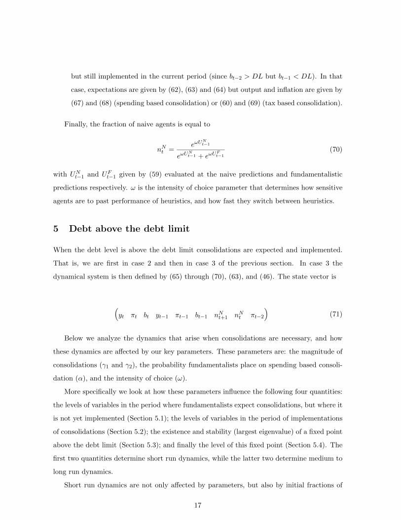
Finally, the fraction of naive agents is equal to
nNt =eωU
Nt−1
eωUNt−1 + eωU
Ft−1
(70)
with UNt−1 and UFt−1 given by (59) evaluated at the naive predictions and fundamentalistic
predictions respectively. ω is the intensity of choice parameter that determines how sensitive
agents are to past performance of heuristics, and how fast they switch between heuristics.
5 Debt above the debt limit
When the debt level is above the debt limit consolidations are expected and implemented.
That is, we are first in case 2 and then in case 3 of the previous section. In case 3 the
dynamical system is then defined by (65) through (70), (63), and (46). The state vector is
(yt πt bt yt−1 πt−1 bt−1 nNt+1 nNt πt−2
)(71)
Below we analyze the dynamics that arise when consolidations are necessary, and how
these dynamics are affected by our key parameters. These parameters are: the magnitude of
consolidations (γ1 and γ2), the probability fundamentalists place on spending based consoli-
dation (α), and the intensity of choice (ω).
More specifically we look at how these parameters influence the following four quantities:
the levels of variables in the period where fundamentalists expect consolidations, but where it
is not yet implemented (Section 5.1); the levels of variables in the period of implementations
of consolidations (Section 5.2); the existence and stability (largest eigenvalue) of a fixed point
above the debt limit (Section 5.3); and finally the level of this fixed point (Section 5.4). The
first two quantities determine short run dynamics, while the latter two determine medium to
long run dynamics.
Short run dynamics are not only affected by parameters, but also by initial fractions of
17
fundamentalists and naive agents. The effects of these initial conditions die out in the long
run.
5.1 Effects of expected consolidations due to a shock to debt or the debt
limit
If in period t debt is above the debt limit for the first time, then in period t+1, consolidations
are expected by fundamentalists, but not yet implemented. The actual type of consolidation
then does not matter yet, but instead dynamics are driven by the type of consolidation
that fundamentalists expect. In Proposition 1 it is stated that depending on what type
fundamentalists expect, a consolidation can both lead to an expansion or a contraction in
output. Furthermore, if the expansion is large enough, expected consolidations lead to a
reduction in debt. Proof of Proposition 1 is given in Appendix A.1.
Proposition 1. Assume that a shock to debt or to the debt limit has increased debt above
its threshold in period t (bt > DLt). This affects next periods output (and thereby also infla-
tion, marginal cost and debt) through fundamentalists’ expectations about future governemnt
spending and future output. The effect of the debt or debt limit shock on next periods output
is given by
∂Yt+1
∂(bt −DLt)= (1− nNt+1)
(η
σ + ηα
γ1
1− g− 1
σ + η
1
1− τ(1− α)γ2
),
This implies that the effect of expected consolidations on output, marginal cost and inflation
is positive, if and only if
αγ1
(1− α)γ2>
1− g1− τ
1
η, (72)
or in terms of the probability they place on a spending based consolidation:
α >γ2(1− g)
γ1(1− τ)η + γ2(1− g)(73)
When this condition does not hold and the expectations lead to a contraction, then expected
consolidation results in an increase in debt. When Condition (72) does hold, the expected
consolidation leads to a reduction in debt if and only if the expansion in output is large
18
enough:
∂Yt+1
∂(bt −DLt)>
1− β
β(
(τ(σ + η)) θ−1θ + b
β (1 + κ(σ + η))) . (74)
It follows from Proposition 1 that it is desirable that agents mainly expect spending
based consolidations. The higher the probability that fundamentalists place on spending
based consolidation, the larger output, and the lower the debt level in the period before the
consolidation is actually implemented. Furthermore, as can be seen in Equation (72), when
fundamentalists do mainly expect spending based consolidations, the expansion in output
and the reduction in debt are increasing in the fraction of fundamentalists (1− nNt+1).
5.2 Effects of implemented consolidations
If after one period debt still is above the debt limit, the expectational effects analyzed above
are still present two periods after the shock. However, in addition there are direct effects of
implemented consolidations on output, inflation and debt. We now turn to the total of these
effects in the period that consolidation is implemented for the first time (two periods after the
shock). Proposition 2 states that in this first consolidation period, a tax based consolidation is
always more effective than a spending based consolidation. Its proof is provided in Appendix
A.2.
Proposition 2. When we assume tax based based and spending based consolidations that
have equal direct impact on the governments budget deficit (γ1 = θ−1θ γ2), then a tax based
consolidation always results in lower debt than a spending based consolidation in the period of
implementation. Moreover, the difference between ∂bt+2
∂(bt−DLt) for spending based and tax based
consolidation is given by
γ1
((τθ − 1
θ+τ θ−1
θ − g1− β
κ)
(θ
(θ − 1)(1− τ)+
η
1− g
)+τ θ−1
θ − g1− β
1
1− g
)(75)
(75) is always positive, so that spending based consolidation indeed always leads to higher
debt than tax based consolidation in the period where it is implemented for the first time. It
can furthermore immediately be seen that the difference in this debt level is increasing the
magnitude of consolidation (γ1 = θ−1θ γ2) and in steady state taxes (τ).
19

5.3 Existence and stability of high debt fixed point
Above we explicitly analyzed the levels of variables in the first two periods after the debt or
debt limit shock. This gives clear insights in the short run dynamics that result form such a
shock. Medium to long run dynamics will be determined by the existence and stability of a
fixed point in the high debt region. In this section we investigate under what conditions this
fixed point exists and how its stability is affected by γ1, γ2, α, and ω (intensity of choice).
5.3.1 Existence
We first consider the two benchmark cases where all agents have correct predictions in the
fixed point. That is, a spending based consolidation with α = 1, and a tax based consolidation
with α = 0. The same fixed point levels can also be obtained with infinite intensity of choice
(ω = +∞). In this limiting case all agents have correct naive expectations in the fixed point.
Stability conditions are then different however, as will be discussed below.
Proposition 3 states when the high debt fixed point lies above the debt limit in case of
spending based consolidation. This is also the condition for the fixed point to exist, since
below the debt limit variables are governed by the low debt dynamical system and not the
high debt system analyzed in this section.
Proposition 3. When consolidations are spending based, and agents expectations are correct
in the high debt fixed point (either because fundamentalists are right, α = 1, or because
ω = +∞ and all agents become naive), then the fixed point lies above the debt limit if and
only if
γ1 >1
β− 1, (76)
Proposition 4 states that in case tax based consolidation the condition for existence of
the high debt fixed point is the same as in case of spending based consolidation, but with γ1
replaced by γ2θ−1θ . This is intuitive because if we let γ1 = γ2
θ−1θ , tax based and spending
based consolidation are of equal magnitude in their effect on the budget deficit.
Proposition 4. When consolidations are tax based, and agents expectations are correct in
the high debt fixed point (either because fundamentalists are right, α = 0, or because ω = +∞
20

and all agents become naive), then the fixed point lies above the debt limit if and only if
γ2θ − 1
θ>
1
β− 1, (77)
5.3.2 Stability
When the fixed point exists in the high debt region it is of interest whether is locally stable,
so that convergence to it can occur. In order to get insight in the stability of the fixed point
for different parameter values we numerically calculate the eigenvalues in the fixed point.
We therefor first need to calibrate the model. Unless otherwise stated we use the parameter
values given in Table 1.
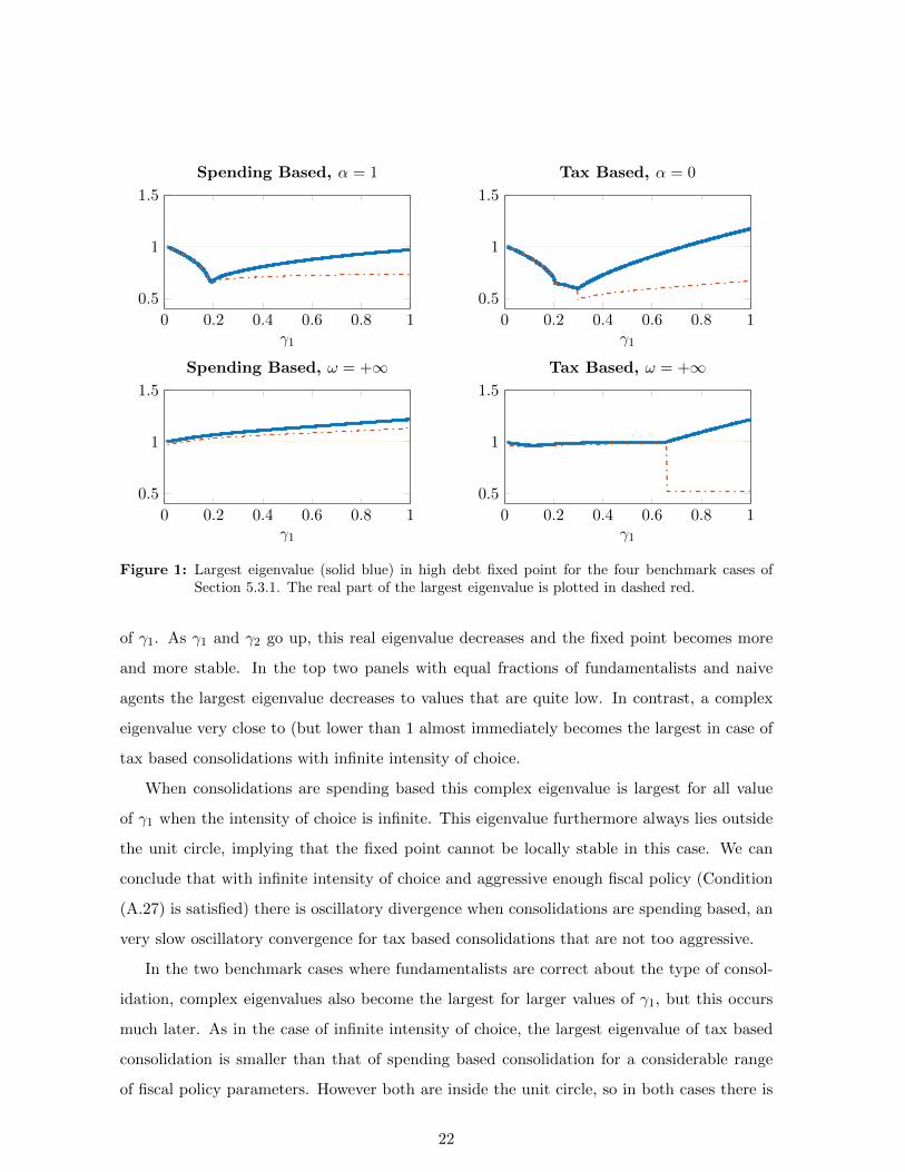
In Figure 1 the largest eigenvalues in the high debt fixed point for spending based (left
panels) and tax based (right panels) are plotted in blue, as a function of γ1 = θ−1θ γ2 (the
magnitude of consolidation). The lower two panels belong to the case of infinite intensity of
choice, where all agents are naive in the fixed point. The top left and top right panel depict
the eigenvalues of the benchmark cases of Proposition 3 and 4 respectively. The real parts
of the largest eigenvalues are plotted in dotted red. When the solid blue and dotted red line
do not coincide, the largest eigenvalue is complex, which implies oscillatory convergence or
divergence.
From the previous section we know that for very low values of γ1 and γ2, the fixed point
does not lie in the high debt region for the four cases plotted in Figure 1. For this reason we
do not plot the largest eigenvalue for γ1 <1β − 1. It can be seen in the Figure, that in 3 of
the four cases the largest eigenvalue is real and equal to unity for the lowest allowed value
Table 1: Parameter values
Parameter Name Valueβ Discount factor 0.99σ Relative risk aversion 21η Frisch elasticity of labor supply 0.5
θ Elasticity of substitution 6φ1 Coefficient on inflation in Taylor rule 1.5ω Intensity of choice 10,000φ Price adjustment costs 100g Steady state government spending 0.21τ Steady state taxes 0.26b Steady state debt 0.66DLt Deviation of debt limit from steady state 0.04
21
0 0.2 0.4 0.6 0.8 1
0.5
1
1.5
γ1
Tax Based, α = 0
0 0.2 0.4 0.6 0.8 1
0.5
1
1.5
γ1
Tax Based, ω = +∞
0 0.2 0.4 0.6 0.8 1
0.5
1
1.5
γ1
Spending Based, α = 1
0 0.2 0.4 0.6 0.8 1
0.5
1
1.5
γ1
Spending Based, ω = +∞
Figure 1: Largest eigenvalue (solid blue) in high debt fixed point for the four benchmark cases ofSection 5.3.1. The real part of the largest eigenvalue is plotted in dashed red.
of γ1. As γ1 and γ2 go up, this real eigenvalue decreases and the fixed point becomes more
and more stable. In the top two panels with equal fractions of fundamentalists and naive
agents the largest eigenvalue decreases to values that are quite low. In contrast, a complex
eigenvalue very close to (but lower than 1 almost immediately becomes the largest in case of
tax based consolidations with infinite intensity of choice.
When consolidations are spending based this complex eigenvalue is largest for all value
of γ1 when the intensity of choice is infinite. This eigenvalue furthermore always lies outside
the unit circle, implying that the fixed point cannot be locally stable in this case. We can
conclude that with infinite intensity of choice and aggressive enough fiscal policy (Condition
(A.27) is satisfied) there is oscillatory divergence when consolidations are spending based, an
very slow oscillatory convergence for tax based consolidations that are not too aggressive.
In the two benchmark cases where fundamentalists are correct about the type of consol-
idation, complex eigenvalues also become the largest for larger values of γ1, but this occurs
much later. As in the case of infinite intensity of choice, the largest eigenvalue of tax based
consolidation is smaller than that of spending based consolidation for a considerable range
of fiscal policy parameters. However both are inside the unit circle, so in both cases there is
22

oscillatory convergence. Furthermore, the eigenvalue of tax based consolidation crosses the
unit circle for a lower value of γ than that of spending based consolidation. For aggressive
policy there thus is oscillatory divergence when fully expected consolidations are tax based,
but oscillatory convergence when they are spending based.
But what can be said about about stability and dynamics when intensity of choice is finite
and α is not equal to 0 ore 1? For arbitrary values of α and ω the fraction of naive agents
in the fixed point will be between 0.5 (as in the top panels) and 1 (as in the bottom panels).
This fraction determines the stability (magnitude of the eigenvalues) of the fixed point. Since
the model is linear in fractions, the fixed point levels of other variables do not show up in
the Jacobian and do not affect stability. The closer α is to the benchmark value, the more
correct fundamentalists are, and the closer the fixed point fraction of naive agents is to 0.5.
The largest eigenvalue is then closer to that of the top panels of Figure 1.
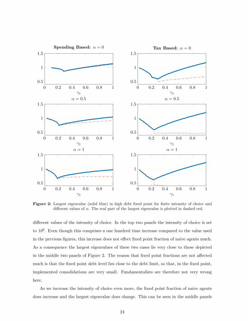
This is illustrated in Figure 2, where the largest eigenvalues for spending and tax based
consolidation are plotted for different values for α. The bottom left and top right panel
correspond to the benchmark cases already depicted in Figure 1. First considering spending
based consolidations (left column of Figure 2) it can be seen that as fundamentalists expect
more tax based consolidations the largest eigenvalue is increased for any value of γ1. These
eigenvalues therefore indeed come closer to the case of all naive agents, depicted in the bottom
left panel of Figure 1. Note that as fundamentalists expect more tax based consolidations,
the range of low γ1 parameters for which the fixed point does not exist becomes larger. The
top left two panels therefore start at higher values of γ1.
Then turning to the right column of tax based consolidations, we see the same pattern.
As fundamentalists expect more spending based consolidations (and therefore become more
wrong), more agents are naive in the fixed point, which leads to larger eigenvalues. The effect
of changing α seems however smaller than in case of spending based consolidation.
When α does not equal the benchmark value the fixed point fraction of naive agents not
only depends on the value of α, but also on the intensity of choice. If the intensity of choice
is zero, the fractions of naive agents always equal 0.5, no matter the value of α. The higher
the intensity of choice, the higher the fixed point fraction of naive agents for any given non
benchmark value of α.
This is illustrated in Figure 3. Here α is set to 0.5 and the largest eigenvalue is plotted for
23
0 0.2 0.4 0.6 0.8 1
0.5
1
1.5
γ1
α = 1
0 0.2 0.4 0.6 0.8 1
0.5
1
1.5
γ1
α = 1
0 0.2 0.4 0.6 0.8 1
0.5
1
1.5
γ1
α = 0.5
0 0.2 0.4 0.6 0.8 1
0.5
1
1.5
γ1
α = 0.5
0 0.2 0.4 0.6 0.8 1
0.5
1
1.5
γ1
Tax Based: α = 0
0 0.2 0.4 0.6 0.8 1
0.5
1
1.5
γ1
Spending Based: α = 0
Figure 2: Largest eigenvalue (solid blue) in high debt fixed point for finite intensity of choice anddifferent values of α. The real part of the largest eigenvalue is plotted in dashed red.
different values of the intensity of choice. In the top two panels the intensity of choice is set
to 106. Even though this comprises a one hundred time increase compared to the value used
in the previous figures, this increase does not effect fixed point fraction of naive agents much.
As a consequence the largest eigenvalues of these two cases lie very close to those depicted
in the middle two panels of Figure 2. The reason that fixed point fractions are not affected
much is that the fixed point debt level lies close to the debt limit, so that, in the fixed point,
implemented consolidations are very small. Fundamentalists are therefore not very wrong
here.
As we increase the intensity of choice even more, the fixed point fraction of naive agents
does increase and the largest eigenvalue does change. This can be seen in the middle panels
24
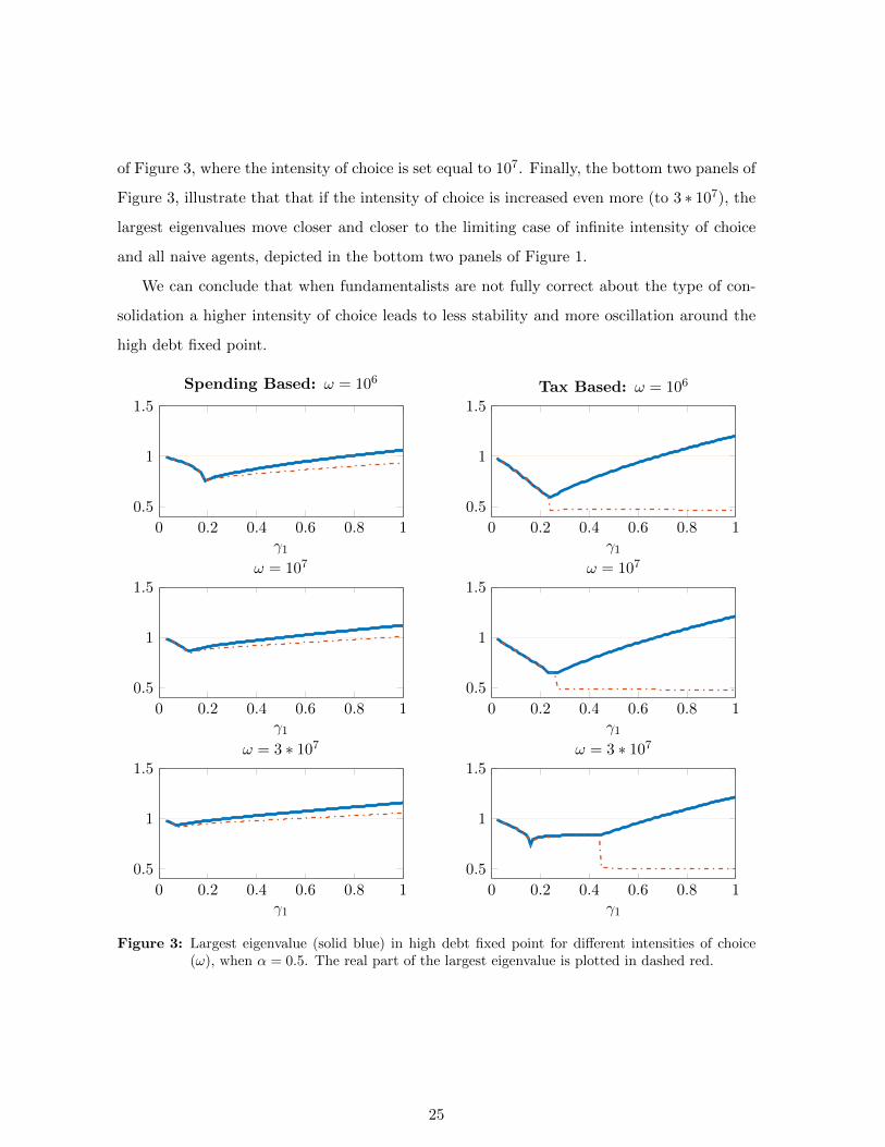
of Figure 3, where the intensity of choice is set equal to 107. Finally, the bottom two panels of
Figure 3, illustrate that that if the intensity of choice is increased even more (to 3 ∗ 107), the
largest eigenvalues move closer and closer to the limiting case of infinite intensity of choice
and all naive agents, depicted in the bottom two panels of Figure 1.
We can conclude that when fundamentalists are not fully correct about the type of con-
solidation a higher intensity of choice leads to less stability and more oscillation around the
high debt fixed point.
0 0.2 0.4 0.6 0.8 1
0.5
1
1.5
γ1
ω = 3 ∗ 107
0 0.2 0.4 0.6 0.8 1
0.5
1
1.5
γ1
ω = 3 ∗ 107
0 0.2 0.4 0.6 0.8 1
0.5
1
1.5
γ1
ω = 107
0 0.2 0.4 0.6 0.8 1
0.5
1
1.5
γ1
ω = 107
0 0.2 0.4 0.6 0.8 1
0.5
1
1.5
γ1
Tax Based: ω = 106
0 0.2 0.4 0.6 0.8 1
0.5
1
1.5
γ1
Spending Based: ω = 106
Figure 3: Largest eigenvalue (solid blue) in high debt fixed point for different intensities of choice(ω), when α = 0.5. The real part of the largest eigenvalue is plotted in dashed red.
25

5.4 Level of the high debt fixed point
When the high debt fixed point is stable, the debt level of this fixed point is of crucial
importance. When this debt level lies very close to the debt limit, the government might
be content with convergence to this fixed point. However, if the debt level lies considerably
above the limit, convergence to the fixed point is not desirable.
The parameters α and ω both affect aggregate expectations in the fixed point. α only
shows up in our model through expectations and its effect on the mode variables can therefore
easily be analyzed. An increase or decrease in α results (for finite intensity of choice) in an
increase or decrease in output.
∂Etgt+1
∂α= −(1− nNt ) (γ1(bt−1 −DL)) < 0 (78)
∂EtYt+1
∂α= (1− nNt )
1
η + σ
(− σ
1− gγ1(bt−1 −DL) +
1
1− τγ2(bt−1 −DL)
)(79)
∂Yt∂α
=
(∂EtYt+1
∂α− 1
1− g∂Etgt+1
∂α
)=∂EtCt+1
∂α=
(1− nNt )
(η
η + σ
γ1
1− g(bt−1 −DL) +
1
η + σ
γ2
1− τ(bt−1 −DL)
)> 0, (80)
Now we know the sign of the effect of a change in α on output we can analyze the effect
of a change in α on the high debt fixed point. When intensity of choice is finite and α is not
equal to the benchmark values analyzed above, the fixed point values for spending and tax
based consolidations are no longer equal to those of the benchmark cases analyzed above.
Because increasing α increases output and does not directly affect any other variable, an
increase in α must increase fixed point output, marginal cost and inflation, and decrease fixed
point debt.
When α is not equal to the benchmark values of the previous subsection the intensity of
choice also affects the fixed point levels. Recall that for infinite intensity of choice the fixed
point levels are as in the benchmark cases, no matter what the values of α is. The lower the
intensity of choice the more the effect of a non-benchmark α is reinforced. For zero intensity
of choice 50% of the agents are fundamentalists and 50% are naive. In this most extreme case
the fixed point lies as far from the benchmark as possible for any given α.
26

Finally we turn to the magnitude of consolidation. From Proposition 3 and 4 it follows
about the benchmark cases that, when the high debt fixed point exists and is stable, more
aggressive policy leads to a lower debt level in the fixed point. We furthermore numerically
find that this result also holds when the intensity of choice is finite and α is not equal to the
benchmark values,
5.5 Comparison spending and tax based consolidations
In this Section we analyze the effect of a shock to the debt limit both in the short run
and in the long run, using impulse responses. We show the difference between spending
based consolidation and tax based consolidation and the difference between strong and weak
responses to debt. We also look how these results depend on agents expectations.
Since our model is linear in expectation fractions, impulse responses are only affected by
the fractions of naive agents in the initial two periods, and not by other initial conditions
(like the level of output when the shock hits). We therefore let the initial fractions of naive
agents vary over a two dimensional grid to obtain both a median impulse response, and an
upper and lower bound on the impulse responses.
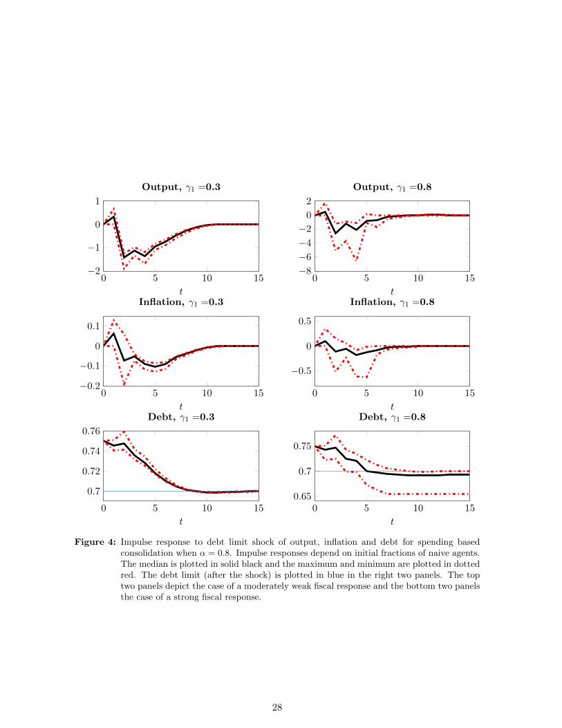
In Figure 4 the impulse responses of output and debt are plotted in case the government
implements spending based consolidation, and fundamentalists also expected mostly spending
based consolidations (α = 0.8). Before period 0 the debt limit was above the debt level, and
from period 0 onward the debt limit is lowered to 70% of GDP, which we assume to be below
the initial debt level of 75% of GDP. The debt limit is indicated by the blue lines in the right
two panels. Black lines indicate median impulse responses, and upper and lower bounds are
given by the dotted red curves.
First consider the left column of panels. Here the reaction coefficient to debt is given
by γ1 = 0.3. In the top left panel we see that in period 1, the period that consolidation is
expected but not yet implemented, a large expansion in output can occur. This is in line with
Proposition 1, since we are considering α = 0.8. As can be seen in Equation 72, the effect of
the shock on output in period 1 is scaled by the fraction of fundamentalists. When all agents
are naive in period 1, nobody expects consolidations to occur in period two and nothing
happens in period 1. When all agents are fundamentalists, everyone expects consolidations
and there is a large expansion in output. This explains why the upper and lower bound lie
27
0 5 10 15
−0.5
0
0.5
t
Inflation, γ1 =0.8
0 5 10 150.65
0.7
0.75
t
Debt, γ1 =0.8
0 5 10 15−8
−6
−4
−2
0
2
t
Output, γ1 =0.8
0 5 10 15−0.2
−0.1
0
0.1
t
Inflation, γ1 =0.3
0 5 10 15
0.7
0.72
0.74
0.76
t
Debt, γ1 =0.3
0 5 10 15−2
−1
0
1
t
Output, γ1 =0.3
Figure 4: Impulse response to debt limit shock of output, inflation and debt for spending basedconsolidation when α = 0.8. Impulse responses depend on initial fractions of naive agents.The median is plotted in solid black and the maximum and minimum are plotted in dottedred. The debt limit (after the shock) is plotted in blue in the right two panels. The toptwo panels depict the case of a moderately weak fiscal response and the bottom two panelsthe case of a strong fiscal response.
28

relatively far apart here. The middle left panel shows that the effect on inflation is similar to
that of output, which also is in line with the theoretical results of Section 5.1. In the bottom
left panel it can be seen that the expansion in output and inflation causes a decline in debt.
However, when all agents were naive, there is no expansion and debt slightly increases in the
first period due to interest rate payments (top red dashed line).
In period 2 government spending is lowered, which leads to a sharp decline in output, and
a (less severe) decline in inflation. This initially causes an increase in debt. However, in the
long run debt decreases towards the high debt fixed point, which lies slightly above the debt
limit. Meanwhile output and inflation converge to their fixed point levels, close to 0. From
Section 5.3.2 we know that for almost fully expected spending based consolidation with low
γ1, the largest eigenvalue in the high debt fixed point will be relatively low. In the top right
panel of Figure 4 we therefore see that debt decreases to a point below the high debt fixed
point, but that it does not overshoot to much. This indicates that the fixed point indeed is
fairly stable.
Turning to the right column of panels of Figure 4, where the policy coefficient is increased
to γ1 = 0.8, we see that there is potentially much more overshooting here. This is in line with
the finding of Section 5.3.2 that the largest eigenvalue is larger here. However, from the large
difference between the two red dashed lines, it can be seen that the amount of overshooting
very much depends on initial fractions of naive agents. Similarly, the qualitative response of
output to the shock is the same as in the case of γ1 = 0.3, but the upper and lower bound
now lie much further apart. We can conclude that in case of mostly expected spending based
consolidation, a stronger response will typically work better than a weak response, but it will
also bring more uncertainty
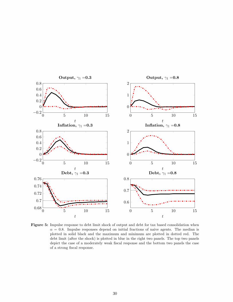
In Figure 5 the impulse responses of a shock to the debt limit are plotted when the gov-
ernemnt implements tax based consolidation, even though agents mostly expected spending
based consolidation (α = 0.8). In period 1 no consolidation is implemented yet, so dynamics
are the same as in Figure 4 (note the difference in scale on te y-axis though). In period 2,
when tax based consolidation is implemented, debt is immediately reduced. This is in line
with Proposition 2, which says that tax based consolidation always initially leads to lower
debt than spending based consolidation. Additionally, we see that there now is no contrac-
tion in output (neither initially nor in the long run), which is also more desirable. Long run
29
0 5 10 15
0
1
2
t
Inflation, γ1 =0.8
0 5 10 15
0.6
0.7
0.8
t
Debt, γ1 =0.8
0 5 10 15
0
1
2
t
Output, γ1 =0.8
0 5 10 15−0.2
0
0.2
0.4
0.6
0.8
t
Inflation, γ1 =0.3
0 5 10 150.68
0.7
0.72
0.74
0.76
t
Debt, γ1 =0.3
0 5 10 15−0.2
0
0.2
0.4
0.6
0.8
t
Output, γ1 =0.3
Figure 5: Impulse response to debt limit shock of output and debt for tax based consolidation whenα = 0.8. Impulse responses depend on initial fractions of naive agents. The median isplotted in solid black and the maximum and minimum are plotted in dotted red. Thedebt limit (after the shock) is plotted in blue in the right two panels. The top two panelsdepict the case of a moderately weak fiscal response and the bottom two panels the caseof a strong fiscal response.
30
debt furthermore is as low or lower as in Figure 4. Overall tax based consolidation clearly is
preferable when agents expect spending based consolidation.
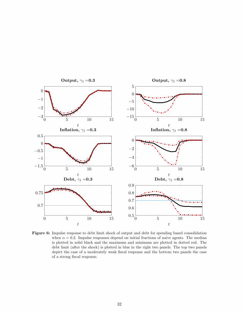
But what if agents mostly expect tax based consolidation? Figures 6 and 7 plot impulse
responses with spending based and tax based consolidation respectively when α = 0.2. First of
all, as predicted by Proposition 1 there is now a contraction instead of an expansion in output
in period 1. Secondly, in Period 2, debt increases in case of spending based consolidation, but
decreases in case of tax based consolidation, in line with Proposition 2.
Spending based consolidation now performs worse then in the case of α = 0.8, both initially
and after a few periods. The cut in government spending leads to a decrease in output that
adds to the contraction already in place because of expectations. This combined effect leads
to a much deeper and longer recession that is accompanied by a high debt level. Only when
output starts to increase again debt decreases towards the debt limit. We furthermore see
that for γ1 = 0.8 debt decreases more sharply than for γ = 0.3, but that the reduction in debt
does not start earlier. The reason for this is that a stronger response to debt also leads to an
even larger contraction in output which prevents policy from effectively controlling debt.
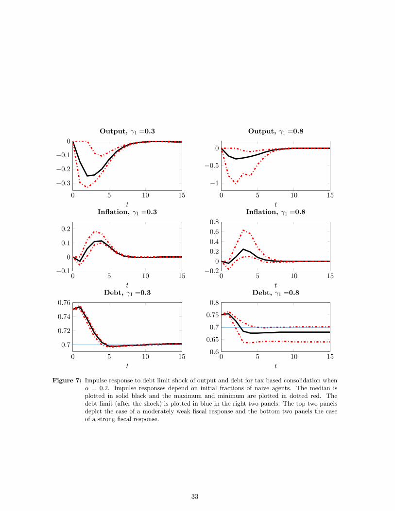
Tax based consolidation on the other hand does not directly depress output. This makes
the contraction caused by expectations much milder, as can be seen by comparing the top
panels of Figure 7 with those of Figure 6. As a consequence debt dynamics turn out not
to be very sensitive to the value of α, as can be seen by comparing the right two panels
of Figure 5 and 7. Our conclusion that tax based consolidation is better than spending
based consolidation thus holds even more strongly when agents mostly expect tax based
consolidation.
31
0 5 10 15−6
−4
−2
0
t
Inflation, γ1 =0.8
0 5 10 150.5
0.6
0.7
0.8
0.9
t
Debt, γ1 =0.8
0 5 10 15−15
−10
−5
0
5
t
Output, γ1 =0.8
0 5 10 15−1.5
−1
−0.5
0
0.5
t
Inflation, γ1 =0.3
0 5 10 15
0.7
0.75
t
Debt, γ1 =0.3
0 5 10 15−3
−2
−1
0
t
Output, γ1 =0.3
Figure 6: Impulse response to debt limit shock of output and debt for spending based consolidationwhen α = 0.2. Impulse responses depend on initial fractions of naive agents. The medianis plotted in solid black and the maximum and minimum are plotted in dotted red. Thedebt limit (after the shock) is plotted in blue in the right two panels. The top two panelsdepict the case of a moderately weak fiscal response and the bottom two panels the caseof a strong fiscal response.
32
0 5 10 15−0.2
0
0.2
0.4
0.6
0.8
t
Inflation, γ1 =0.8
0 5 10 150.6
0.65
0.7
0.75
0.8
t
Debt, γ1 =0.8
0 5 10 15
−1
−0.5
0
t
Output, γ1 =0.8
0 5 10 15−0.1
0
0.1
0.2
t
Inflation, γ1 =0.3
0 5 10 15
0.7
0.72
0.74
0.76
t
Debt, γ1 =0.3
0 5 10 15
−0.3
−0.2
−0.1
0
t
Output, γ1 =0.3
Figure 7: Impulse response to debt limit shock of output and debt for tax based consolidation whenα = 0.2. Impulse responses depend on initial fractions of naive agents. The median isplotted in solid black and the maximum and minimum are plotted in dotted red. Thedebt limit (after the shock) is plotted in blue in the right two panels. The top two panelsdepict the case of a moderately weak fiscal response and the bottom two panels the caseof a strong fiscal response.
33
6 Conclusions
In this paper we have explored the effects of fiscal consolidations when agents are heteroge-
neous and uncertain about the composition of the consolidations. We assumed agent hetero-
geneity in the way expectations are formed in the spirit of Brock and Hommes (1997). Agents
can switch between two types, namely, the fundamentalist and the naive. The former type
consisted of forward looking agents, whereas the latter consisted of backward looking agents.
The Fiscal authority was assumed to engineer a consolidation once debt exceeds an an-
nounced debt limit, with a lag. Consolidations were implemented either through spending
cuts or tax increases. Prior to the consolidation agents were uncertain about the composi-
tion. Given the lag in implementation, such uncertainty affected only the way fundamentalists
formed their expectations leaving the expectations of naive agents unaffected.
Our first finding was that tax-based consolidations outperform spending-based ones in the
short-run leading to an abrupt fall in the debt-to-GDP ratio. We showed that the type of
consolidation anticipated was crucial at determining whether the consolidation would trigger
expansions or abrupt contractions in output so long as it lasts. Moreover, whether the type
of consolidation anticipated was correct or not, determined its duration. Consolidations last
longer as long as agents wrongly anticipate them to be tax-based, but turn out to be spending
based. This is due to the persistent contraction in output triggered by the the spending cuts
and the rise in real interest rates due to inflationary pressures.
Interestingly, in the medium to long-run it is ambiguous which type of consolidation is
more successful in stabilizing the debt ratio. Spending based consolidations of high magnitude
tend to outperform tax-based ones, when agents anticipate the latter to occur. The model
was complex in its dynamics and we kept the analysis as simple as possible. Cases like the
effect of the zero lower bound on the potential of a consolidation to be expansionary and/or
successful in stabilizing debt, in a heterogeneous agents model, deserve further research.
34

A Proofs of propositions
A.1 Proof Proposition 1
∂Et+1gt+2
∂(bt −DLt)= −(1− nNt+1)αγ1 (A.1)
∂Et+1Yt+2
∂(bt −DLt)= −(1− nNt+1)
1
σ + η
(σ
1− gαγ1 +
1
1− τ(1− α)γ2
)< 0 (A.2)
∂Yt+1
∂(bt −DLt)=
(∂Et+1Yt+2
∂(bt −DLt)− 1
1− g∂Et+1gt+2
∂(bt −DLt)
)=
∂Et+1Ct+2
∂(bt −DLt)=
(1− nNt+1)
(η
σ + ηα
γ1
1− g− 1
σ + η
1
1− τ(1− α)γ2
), (A.3)
It follows that the effect of a debt (or debt limit) shock on next periods output (and
marginal cost and inflation) is positive, if and only if
ηαγ11
1− g>
1
1− τ(1− α)γ2
αγ1
(1− α)γ2>
1− g1− τ
1
η(A.4)
When α = 1 this will always hold and when α = 0 it will never hold. Solving for α gives
α >γ2(1− g)
γ1(1− τ)η + γ2(1− g)
Next we turn the the effect of a debt shock on debt on the other variables of the model.
We first of all have
∂πt+1
∂(bt −DLt)= κ(σ + η)
∂Yt+1
∂(bt −DLt)(A.5)
∂mct+1
∂(bt −DLt)= (σ + η)
∂Yt+1
∂(bt −DLt)(A.6)
35

For debt we have
∂bt+1
∂(bt −DLt)=
1
β− τ θ − 1
θ
∂mct+1
∂(bt −DLt)− b
β
∂Yt+1
∂(bt −DLt)− b
β
∂πt+1
∂(bt −DLt)(A.7)
=1
β−(
(τ(σ + η))θ − 1
θ+b
β(1 + κ(σ + η))
)∂Yt+1
∂(bt −DLt)(A.8)
We can conclude that if (A.4) is not satisfied (and a higher debt level leads to a lower output
level then an increase in bt−1 implies a more than one for one increase in bt, so that bt > bt−1
and consolidation expectations lead to an increase in debt.
If (A.4) is satisfied, then the expectations of consolidations may reduce period t+ 1 debt
compared to period t debt. This happens if and only if
∂bt+1
∂(bt −DLt)=
1
β−(
(τ(σ + η))θ − 1
θ+b
β(1 + κ(σ + η))
)∂Yt+1
∂(bt −DLt)< 1 (A.9)
∂Yt+1
∂(bt −DLt)>
1− β
β(
(τ(σ + η)) θ−1θ + b
β (1 + κ(σ + η))) (A.10)
A.2 Proof Proposition 2
We first assume spending based consolidation.
Fundamentalists only base their expectations on bt−1 and not on bt−2 debt, so from them
there is only an indirect effect of bt−2 on period t variables. However, naive agents base their
expectations on lagged variables, that do depend on bt−2 in the way analyzed in the previous
section.
We therefore have
∂Yt+2
∂(bt −DLt)=∂Yt+2
∂bt+1
∂bt+1
∂(bt −DLt)− 1
1− gγ1 + nNt+2
∂Yt+1
∂(bt −DLt)− φ1 − 1
σnNt+2
∂πt+1
∂(bt −DLt)(A.11)
∂πt+2
∂(bt −DLt)=∂πt+2
∂bt+1
∂bt+1
∂(bt −DLt)+σκγ1
1− g+ βnNt+2
∂πt+1
∂(bt −DLt)+ κ(σ + η)
∂Yt+2
∂(bt −DLt),(A.12)
∂mct+2
∂(bt −DLt)=∂mct+2
∂bt+1
∂bt+1
∂(bt −DLt)+
σγ1
1− g+ (σ + η)
∂Yt+2
∂(bt −DLt)(A.13)
36
where ∂Yt+2
∂bt+1is obtained by replacing nNt+1t by nNt+2 in (A.3). Updating (A.5) and (A.6)
accordingly gives the other derivatives.
Finally, we have
∂bt+2
∂(bt −DLt)= −γ1 +
1
β
∂bt+1
∂(bt −DLt)− τ θ − 1
θ
∂mct+2
∂(bt −DLt)+b
β
(∂Yt+1
∂(bt −DLt)− ∂Yt+2
∂(bt −DLt)− ∂πt+2
∂(bt −DLt)
)= −γ1 +
1
β
∂bt+1
∂(bt −DLt)−(τθ − 1
θ+b
βκ
)σγ1
1− g−(τθ − 1
θ(σ + η) +
b
βκ(σ + η)
)∂Yt+2
∂bt+1
∂bt+1
∂(bt −DLt)
−(
(τ(σ + η))θ − 1
θ+b
β(1 + κ(σ + η))
)∂Yt+2
∂(bt −DLt)+b
β
(1− βnNt+2κ(σ + η)
) ∂Yt+1
∂(bt −DLt)(A.14)
In case of tax based consolidation we get
∂Yt+2
∂(bt −DLt)=∂Yt+2
∂bt+1
∂bt+1
∂(bt −DLt)+ nNt+2
∂Yt+1
∂(bt −DLt)− φ1 − 1
σnNt+2
∂πt+1
∂(bt −DLt)(A.15)
∂πt+2
∂(bt −DLt)=∂πt+2
∂bt+1
∂bt+1
∂(bt −DLt)+
κγ2
1− τ+ βnNt+2
∂πt+1
∂(bt −DLt)+ κ(σ + η)
∂Yt+2
∂(bt −DLt),(A.16)
∂mct+2
∂(bt −DLt)=∂mct+2
∂bt+1
∂bt+1
∂(bt −DLt)+
γ2
1− τ+ (σ + η)
∂Yt+2
∂(bt −DLt)(A.17)
Finally, we have
∂bt+2
∂(bt −DLt)=
−θ − 1
θγ2 +
1
β
∂bt+1
∂(bt −DLt)− τ θ − 1
θ
∂mct+2
∂(bt −DLt)+b
β
(∂Yt+1
∂(bt −DLt)− ∂Yt+2
∂(bt −DLt)− ∂πt+2
∂(bt −DLt)
)= −θ − 1
θγ2 +
1
β
∂bt+1
∂(bt −DLt)−(τθ − 1
θ+b
βκ
)γ2
1− τ−(τθ − 1
θ(σ + η) +
b
βκ(σ + η)
)∂Yt+2
∂bt+1
∂bt+1
∂(bt −DLt)
−(
(τ(σ + η))θ − 1
θ+b
β(1 + κ(σ + η))
)∂Yt+2
∂(bt −DLt)+b
β
(1− βnNt+2κ(σ + η)
) ∂Yt+1
∂(bt −DLt)(A.18)
The difference between spending based and tax based second period debt is
−(γ1 −θ − 1
θγ2)− (τ
θ − 1
θ+b
βκ)(
σγ1
1− g− γ2
1− τ) +
((τ(σ + η))
θ − 1
θ+b
β(1 + κ(σ + η))
)γ1
1− g
assuming consolidations of equal impact on the budget deficit (γ1 − θ−1θ γ2), this reduces
37

to
γ1
((τθ − 1
θ+b
βκ)(
θ
(θ − 1)(1− τ)− σ
1− g) +
((τ(σ + η))
θ − 1
θ+b
β(1 + κ(σ + η))
)1
1− g
)(A.19)
We can rewrite this as
γ1
((τθ − 1
θ+b
βκ)
(θ
(θ − 1)(1− τ)+
η
1− g
)+b
β
1
1− g
)(A.20)
This implies that a spending based consolidation leads to a higher debt then a tax based
consolidation after two periods. Substituting for steady state debt we get
γ1
((τθ − 1
θ+τ θ−1
θ − g1− β
κ)
(θ
(θ − 1)(1− τ)+
η
1− g
)+τ θ−1
θ − g1− β
1
1− g
)(A.21)
We can conclude that the difference between spending based and tax based in the second
period is increasing in: the magnitude of consolidation (γ1), steady state taxes (τ). The
relation with steady state government spending is not immediately clear.
A.3 Proof Proposition 3
We assume steady state levels and we assume a spending based consolidation is implemented.
In a fixed point where both fundamentalists and naive agents are correct (because α = 1)
inflation and output satisfy
π(1− βnN ) = κ(σ + η)Y + κσγ1(b−DL)
1− g(A.22)
(1− nNt )Y = −(1− nNt )1
η + σσγ1(b−DL)
1− g− φ1 − 1
σnNt π. (A.23)
Solving this two equations shows that fixed point inflation and marginal cost are zero and
fixed point output is given by the fundamentalists expected value:
Y = − 1
η + σσγ1(b−DL)
1− g, (A.24)
When fundamentalists are wrong (α 6= 1), but the intensity of choice is infinite (ω = +∞),
then in the fixed point nNt = 1. In this case the fixed point levels of output, inflation and
38

marginal cost are the same as above.
For debt we have in the fixed point where marginal cost and inflation are zero:
b = −γ1(b−DL) +1
βb, (A.25)
The fixed point debt level therefore is
b =DLγ1
1− 1β + γ1
(A.26)
This is indeed a fixed point when the fixed point debt level lies above the debt limit. This is
the case if and only if
γ1 >1
β− 1, (A.27)
A.4 Proof Proposition 4
In the benchmark case of tax based consolidations that are fully expected by fundamentalists
(α = 0) we again have a fixed point where marginal cost and inflation are zero. Output is
now given by
Y = − 1
η + σ(γ2(b−DL)
1− τ),
For infinite intensity of choice the same fixed point is reached, but with all naive expectations.
For debt we now have
b =DLγ2
θ−1θ
1− 1β + γ2
θ−1θ
(A.28)
This is indeed a fixed point when this debt level lies above the debt limit
The condition now becomes
γ2θ − 1
θ>
1
β− 1, (A.29)
39
References
Alesina, Alberto and Roberto Perotti (1995), Fiscal Expansions and Fiscal Adjustments in
OECD Countries, NBER Working Papers 5214, National Bureau of Economic Research,
Inc.
Alesina, Alberto and Silvia Ardagna (1998), ‘Tales of fiscal adjustment’, Economic Policy
13(27), 487–545.
Alesina, Alberto and Silvia Ardagna (2010), Large Changes in Fiscal Policy: Taxes versus
Spending, in ‘Tax Policy and the Economy, Volume 24’, NBER Chapters, National Bureau
of Economic Research, Inc, pp. 35–68.
Ardagna, Silvia (2004), ‘Fiscal stabilizations: When do they work and why’, European Eco-
nomic Review 48(5), 1047–1074.
Bi, Huixin, Eric M. Leeper and Campbell Leith (2013), ‘Uncertain fiscal consolidations’, The
Economic Journal 123(566).
Brock, William and Cars Hommes (1997), ‘A rational route to randomness’, Econometrica
65(5), 1059–1096.
IMF (2011), ‘Shifting gears: Tackling challenges on the road to fiscal adjustment’, 51(0), 180
– 203.
Perotti, Roberto (1996), ‘Fiscal consolidation in europe: Composition matters’, The American
Economic Review 86(2), pp. 105–110.
40