expectations, heterogeneous forecast errors, and...
TRANSCRIPT

NICHOLAS S. SOULELES
Expectations, Heterogeneous Forecast Errors,
and Consumption: Micro Evidence from
the Michigan Consumer Sentiment Surveys
The household data underlying the Michigan Index of Consumer Sentimentare used to test the rationality of consumer expectations and their usefulnessin forecasting expenditure. The results can be interpreted as characterizingthe shocks that hit different types of households over time. Expectationsare found to be biased and inefficient, at least ex post. People underestimatedthe disinflation of the early 1980s and the severity of recent businesscycles. People’s forecast errors are also systematically correlated with theirdemographic characteristics, in part because of time-varying, group-levelshocks. Further, sentiment helps forecast consumption growth. Some ofthis rejection of the permanent income hypothesis is due to the systematicdemographic components in forecast errors.
JEL code: E21Keywords: consumer sentiment, consumer confidence, permanent incomehypothesis, excess sensitivity, precautionary saving, subjective expectations,
rational expectations, forecast errors, shocks, unobserved heterogeneity.
Debate over the usefulness of consumer sentiment surveysin forecasting economic activity began soon after their introduction in the 1940s. Thepossibility that a decline in consumer confidence helped cause or worsen the 1990–91 recession renewed interest in the debate. Most recent studies of sentiment have
For helpful comments the author thanks two anonymous referees, Martin Browning, Chris Carroll,Roger Ferguson, Todd Sinai, Sarah Tanner, and seminar participants at Rutgers, the Federal ReserveBank of Philadelphia, the Michigan/HRS/BLS Conference on Survey Research on Household Expectationsand Preferences, Chicago, Princeton, Tilburg, the Federal Reserve Board of Governors, McMaster, York,the NBER summer workshop and the Wharton macro lunch. I am very grateful to Richard Curtin forproviding data and feedback, to Hoon Ping Teo for excellent research assistance, and for financial supportto the Rodney L. White Center for Financial Research. Of course, none of these people is responsiblefor any errors herein. An earlier version of this paper circulated under the title “Consumer Sentiment:Its Rationality and Usefulness in Forecasting Expenditure—Evidence from the Michigan Micro Data”.
Nicholas S. Souleles is an associate professor at the Finance Department of theUniversity of Pennsylvania and NBER. E-mail: souleles�wharton.upenn.edu
Received March 23, 2000; and accepted in revised form May 14, 2002.
Journal of Money, Credit, and Banking, Vol. 36, No. 1 (February 2004)Copyright 2004 by The Ohio State University
40 : MONEY, CREDIT, AND BANKING
focused on the time-series relationship between aggregate consumption and the twomain aggregate indices of sentiment, the Michigan Index of Consumer Sentiment(ICS) and the Conference Board Consumer Confidence Index. This paper, bycontrast, provides perhaps the first comprehensive analysis of the household-leveldata that underlies the ICS, the Michigan Survey of Consumer Attitudes and Behavior(CAB). The attention that the ICS receives, from policymakers, academics, and thebusiness community, itself warrants an analysis of the underlying data. There are alsoa number of methodological advantages to such an analysis.
First, with micro data one can assess the rationality of household expectations.Most previous rationality tests have limited their focus to inflation expectations, justone of the many variables that will be examined here. Also, the tests have generallyused aggregated data or at most short micro panels. But when agents’ informationsets differ, aggregation can lead to spurious rejections of rationality. The averageof rational individual forecasts need not be a rational forecast conditional on anysingle information set (Keane and Runkle 1990). And, even if individual forecastsare perfectly rational, it might take a long time—perhaps multiple business cycles—for forecast errors to average out. Hence, to test rationality, it is important to usemicro data on expectations over long sample periods. Unfortunately, such dataare not usually available. The CAB survey, however, is unique in containing almost20 years of monthly household expectations data. This paper exploits its panelaspect to test more cleanly than usual whether expectations are unbiased and efficient.The results can also be interpreted as explicitly characterizing the time-series andcross-sectional properties of the shocks that have hit different types of householdsover time, across business cycles, and policy regimes. In addition to its welfareimplications, such a characterization is of methodological interest because boththeoretical and empirical models are generally sensitive to the assumptions madeabout shock processes. In particular, many models assume that “aggregate” shocksaffect all households equally.
Second, this paper assesses whether the sentiment surveys are useful in predictingbehavior, specifically household spending. The canonical permanent income (or lifecycle) hypothesis (PIH) provides a natural setting for this assessment. One ofthe central implications of the PIH is that current consumption should incorporateall the information available to an agent. However, the econometrician does notindependently observe the contents of agents’ information sets, so tests of thisimplication usually need to make strong assumptions, inferring agents’ expecta-tions econometrically. This paper instead uses direct measures of expectationsfrom the CAB data. This data is matched, using a rich set of demographicvariables, with the Consumer Expenditure Survey (CEX), which has the most com-prehensive micro data on expenditure. The resulting test is whether the expectationsdata contain additional information, beyond that in current consumption, thathelps predict future consumption. Previous studies of the excess sensitivity of

NICHOLAS S. SOULELES : 41
consumption to sentiment have used aggregate sentiment data but aggregation caninduce spurious excess sensitivity even when there is none at the micro level(Attanasio and Weber 1995). The construction of the ICS is not necessarily consistentwith the construction of aggregate consumption. For instance, the ICS is an equal-weighted average of the sentiment of the CAB survey respondents, which ignoresdifferences in the scale of consumption across respondents.
With micro data, one can also more readily investigate the sources of any excesssensitivity. One alternative hypothesis that has not previously received much scrutinyis that forecast errors might not be classical but rather contain systematic componentscorrelated with the excess sensitivity regressor. For instance, over the sample period,high-income households might on average have been optimistic about the future,and might have happened to receive disproportionately positive shocks. In thiscase, increases in their consumption and so a positive correlation between consump-tion and sentiment would not be inconsistent with the PIH. More broadly, Chamberlain(1984) and others have pointed out that systematic forecast errors can be a potentialproblem in estimating any rational expectations (or forward-looking) model in ashort panel. Because direct measures of households’ forecast errors are availablehere, it is possible to test this point directly.
Third, the aggregate ICS ignores potentially useful information available in themicro CAB data. As already noted, the ICS neglects the cross-sectional distributionof sentiment. This distribution might be useful in predicting the expenditure ofdifferent groups of consumers or even aggregate expenditure insofar as the relationbetween expenditure and sentiment at the household level does not aggregate up.In the ICS, a given respondent’s sentiment is in turn the sum of her answers to fivevery different survey questions, which makes it hard to interpret. This paper exam-ines, separately for each question, whether the survey responses help forecasthousehold spending. This examination also addresses one perennial question in theforecasting literature: Does sentiment provide information useful in forecastingabove and beyond the information contained by other available macro variables likestock prices? By controlling for time effects in the micro data, one can exploitpurely cross-sectional variation that is orthogonal to any macro variable.
To preview the results, expectations appear to have been biased, at least ex post,in that forecast errors did not average out even over a long sample period lastingalmost 20 years. This bias is not constant over time; it is related to the inflationregime and the business cycle. People underestimated the disinflation of the early1980s and in the 1990s and generally appear to underestimate the severity ofbusiness cycles. Expectations are also inefficient, in that people’s forecast errorswere correlated with their demographic characteristics. That is, forecast errors aresystematically heterogeneous. The results suggest an important role for time-varying,group-level shocks—aggregate shocks do not hit all people equally. For instance,during recent expansions high-income households received relatively good shocks
42 : MONEY, CREDIT, AND BANKING
but low-income households continued to receive somewhat negative shocks onbalance, consistent with ongoing, unexpected skill-biased technical change. Further,sentiment is useful in forecasting future consumption, even beyond lagged consump-tion and other macro variables, counter to the PIH. Higher confidence is correlated withless saving, consistent with precautionary motives and increases in expected futureresources. Some of the rejection of the PIH is found to be due to the systematicdemographic components in forecast errors. But even after controlling for thesecomponents, some excess sensitivity persists. More broadly, because forecast errorsare correlated with household demographic characteristics, they will be correlatedwith many regressors of interest in forward-looking models. This suggests thatsystematic heterogeneity in forecast errors is in practice a general problem.
The paper begins by surveying related studies in Section 1. Section 2 describes thedata and Section 3, the econometrics. Section 4 tests the rationality of expectations andmore generally characterizes the properties of forecast errors. Section 5 tests whethersentiment helps forecast expenditure, and if so, whether this is due to systematicheterogeneity in forecast errors. Section 6 concludes.
1. RELATED STUDIES
Most tests of the rationality of surveyed expectations have focused on inflationexpectations of economists (e.g., Keane and Runkle 1990). A few studies haveexamined the inflation expectations of consumers in general, using the aggregatedMichigan data (e.g., Maddala, Fishe, and Lahiri, 1981, Gramlich, 1983, Batchelor,1986). These studies mostly analyzed the Michigan question that allows only discrete,qualitative responses about the future path of inflation (up/down/no change). Touse this question quantitatively, the studies typically made strong assumptionsto derive a continuous-valued expectations time-series from the Michigan data.Moreover, as already noted, because of aggregation bias, the implications of thesetests for individual rationality are not straightforward. One study, Batchelor andJonung (1989), examined micro-level data on the inflation expectations of a smalland short (one year) Swedish panel, finding evidence of bias and inefficiency.However, rationality does not require that people’s expectations be on target overthe course of only a single year.
Flavin (1991) and Alessie and Lusardi (1997) used micro-level data on incomeexpectations to predict future income. While they did not formally test the rationalityof these expectations, they did find a positive, if not very large, correlation betweenthem and future realizations of income (see also Domnitz 1988). More recently,an interesting paper by Das and van Soest (1999) tested the rationality of incomeexpectations in a Dutch dataset. They found that income expectations were onaverage too low relative to subsequent realizations. However, their data is alsolimited to a relatively short panel (1984–88). As shown below, even five years

NICHOLAS S. SOULELES : 43
might be too few to allow forecast errors to average out. Expectations mighthave been rational ex ante, but might not appear rational ex post. For instance, thesample might by chance have received unexpectedly good income realizations overthe period. This paper, by contrast, uses almost 20 years of micro data for manydifferent kinds of expectations questions. Of course, even 20 years might not be along enough period. But such a result would be as significant as a finding ofirrationality because most micro studies are limited to datasets with a shortersample period.
Even if expectations are not fully classical, people might still act on them andso they might help forecast spending. Of particular interest is whether sentimentsurveys contain predictive information not available in other variables, most salientlycurrent consumption. Two interesting papers have examined this issue using aggre-gate time-series data, in an Euler-equation framework.1 Carroll, Fuhrer, and Wilcox(1994) used the ICS and Acemoglu and Scott (1994) used a similar Gallup poll inBritain. Both found significant excess sensitivity of consumption to sentiment andsuggested that sentiment might be picking up precautionary motives. But under thisinterpretation, the sign of their estimated excess sensitivity is somewhat surprising:increased confidence led to a steeper consumption profile, i.e., to increasedsaving; whereas the simplest precautionary model would have increased confidencelead to less saving.2,3 Also, it remains an open question whether other variablesmight already incorporate the information in aggregate sentiment. While Carroll,Fuhrer, and Wilcox show that the ICS contains additional information beyond thatavailable in aggregate income, other studies have found that financial variables, inparticular stock prices, significantly reduce the contribution of aggregate sentimentin forecasting (Friend and Adams, 1964, Ludvigson, 1996). By revisiting the matterusing micro data, this paper avoids potential aggregation bias and takes advantageof additional information in the cross-sectional distribution of sentiment.
Only a few papers have used micro-level expectations data in an Euler-equationframework.4 Two of the most interesting are by Flavin (1991) and Alessie andLusardi (1997), who used income expectations as instruments for income in the
1. The earliest study of which I am aware that used an Euler equation framework to analyze sentimentis an unpublished Federal Reserve Board working paper by Burch and Gordon (1985), again usingaggregate data. The Gulf War triggered a number of additional studies of aggregate sentiment, often byresearchers in the Federal Reserve System (e.g., Throop, 1992, and Carroll, Fuhrer, and Wilcox, 1994).
2. A steeper consumption profile implies increased saving under the null hypothesis of the PIH.Outside the PIH, this implication need not hold.
3. Carroll, Fuhrer, and Wilcox (1994) note that frictions in consumption, e.g., due to habits, canpotentially explain the sign of their results. Acemoglu and Scott (1994) suggest a different explana-tion: higher confidence might be correlated with higher levels of income, which in turn might be correlatedwith a higher variance in income, and so a greater precautionary motive.
4. Some of the earliest studies of sentiment, in the 1950s and 1960s, also used micro data. Theirresults were mixed. (See McNeil (1974) for a summary.) They generally had small sample sizes andshort time horizons. Further, it is often difficult to interpret their results because the models of consumptionthey used are generally different from current models. Outside the consumption literature, Nicholson andSouleles (2002a, 2002b) find that income expectations of medical students help predict their specialtychoice and subsequent practice behavior. They also trace the source of physicians’ forecast errors toparticular shocks to their practices and health-care market, such as the emergence of HMOs.

44 : MONEY, CREDIT, AND BANKING
related Euler equation for saving. Both rejected the PIH. However, both studieswere limited to essentially single cross sections (the 1967 SCF and a 1986 Dutchpanel, respectively), leaving systematic heterogeneity in forecast errors a potentialproblem.5 To illustrate, Mariger and Shaw (1993) showed that in the Panel Studyof Income Dynamics the excess sensitivity coefficient on lagged income growthvaries in sign from year to year. For instance, the three-year sample used by Halland Mishkin (1982) yields a negative coefficient, but other short samples yield apositive coefficient. Mariger and Shaw conjectured that this instability might be dueto aggregate shocks. But in contrast to this paper, without an independent measure ofthese shocks they were unable to test their conjecture directly.
2. DATA
2.1. The Michigan Survey of Consumer Attitudes and Behavior
The CAB is a nationally representative survey that since 1978 has been conductedmonthly. This paper uses the data from December 1978 through June 1996. Inrecent years, about 500 households are sampled each month, in the earlier yearstwo to three times as many were sampled. The five questions that comprise the widelyfollowed ICS are as follows. The allowed responses are in brackets (underlining inoriginal).
QFPr. (Financial Position realization) We are interested in how people are gettingalong financially these days. Would you say that you (and your family living there)are better off or worse off financially than you were a year ago? [better now, same,worse now]
QFPe. (Financial Position expectation) Now looking ahead—do you think that ayear from now you (and your family living there) will be better off financially orworse off, or just about the same as now? [will be better off, same, will be worse off]
QBC. (Business Conditions) Now turning to business conditions in the countryas a whole—do you think that during the next 12 months we’ll have good timesfinancially, or bad times, or what? [good times, good times with qualifications, pro-con, bad with qualifications, bad times]
QBC5. (Business Conditions, five-year horizon) Looking ahead, which wouldyou say is more likely—that in the country as a whole we’ll have continuousgood times during the next 5 years or so, or that we will have periods of widespreadunemployment or depression, or what? [good times, good times qualified, pro-con,bad times qualified, bad times]
QDP. (Durables Purchases) About the big things people buy for their homes—such as furniture and refrigerator, stove, television, and things like that. Generallyspeaking, do you think now is a good or bad time for people to buy major householditems? [good, pro-con, bad]
5. A recent paper by Jappelli and Pistaferri (2000) uses a few cross sections of income expectationsfrom an Italian Survey in an Euler equation. While they do not find excess sensitivity, they note this mightbe due to measurement error, especially in the timing of their expectational questions vis-a-vis theother variables.

NICHOLAS S. SOULELES : 45
Some economists are wary of subjective survey questions. Instead of reviewingtheir generic advantages and disadvantages or offering an exegesis of these particularquestions, this paper will formally test the rationality of the responses to the questionsand see whether they are correlated with behavior, specifically whether they helpforecast spending.6,7 In a related paper, Souleles (2001) shows that these samequestions help predict household purchases of risky securities. Even controlling forpast stock returns, households that are pessimistic about the future buy fewer riskysecurities, ceteris paribus.8
A few additional notes are in order. First, questions QBC, QBC5, and QDP askthe respondent about aggregate economic activity, while QFPr and QFPe ask aboutthe household’s own financial position. This difference suggests there might bemore cross-sectional variation in QFPr and QFPe than in the other variables. Second,QFPe, QBC, and QBC5 ask about the future9, whereas QFPr asks about the pastyear and QDP asks about the present. Third, the wording of QFPe (“e” for expecta-tion) matches that of QFPr (“r” for realization). Thus if someone is asked QFPe thisyear, and then QFPr next year, QFPe provides a forecast of what his answer to QFPr
will be. However, the response to QFPe is constrained to fall in one of three categories(better, worse, or the same). Therefore the analysis will accommodate the discrete,ordered nature of this and the other variables. For convenience, the better states(“better” or “good” or “good with qualification”) are usually coded as �1, theintermediate states (“same” or “pro-con”) as 0, and the worse states (“worse” or“bad” or “bad with qualification”) as �1.10
Figures 1 and 2 show the average response for each question month-by-month.All five variables are procyclical. Notably, the forward-looking expectational vari-able QFPe appears to lead the backward-looking realization QFPr. For instance,QFPe recovers more quickly from both the 1980–81 recession and the 1990 invasionof Kuwait. Nonetheless, the two aggregate time series are highly correlated, atabout 0.8.
The CAB survey asks many additional questions. This paper highlights the fivequestions above because they comprise the ICS but will also consider the mostsalient of the additional questions, listed in Appendix A. There are two matching
6. As for the particular wording of these questions, they have the virtue of having stayed the sameover the sample period. Also, it is worth noting that most household-level data, not just sentiment, isself-reported by households.
7. Carroll, Fuhrer, and Wilcox (1994) and others have shown that the aggregate ICS helps forecastaggregate consumption.Studies of the CAB inflation expectations, described below, have found that they arehelpful in predicting CPI inflation, sometimes performing better than inflation forecasts from professionalforecasters (Thomas 1999).
8. For another application of the CAB, to tax cuts, see Shapiro and Slemrod (1995).9. These three questions make up the Expectations subindex of the ICS, which in turn is a component
of the Index of Leading Economic Indicators.10. The ICS uses this coding in a diffusion index. For each question, the aggregate value at a given
time is the number of people answering �1 at that time minus the number of people answering �1.Such indexes omit the people answering 0, as well as the distribution of the rest of the answers acrosspeople of different characteristics.

46 : MONEY, CREDIT, AND BANKING
Fig. 1. Monthly means of the household financial position variables QFPr and QFPe. For the realizations questionQFPr, responses were coded as �1 if the household’s financial position is better now than a year ago, �1 if it is worsenow, and 0 if it is about the same. For the expectations question QFPe, responses were coded as �1 if its financialposition is expected to be better a year from now, �1 if expected to be worse, and 0 if expected to be about the same.
questions on business conditions similar to QBC. Since one can be taken as theexpectation of the other, they will be denoted QBCe and QBCr. There are alsomatched questions about changes in prices, QPe and QPr, and changes in the house-hold’s real income, QYe and QYr, over the following year and previous year,respectively. QUe asks whether the respondent expects the national unemploymentrate to increase or decrease over the next year. Even though there is no matching real-ization question about perceived changes in unemployment over the past year, thisquestion is used because precautionary saving might be sensitive to unemploymentexpectations.11 The answers to all these questions are again discrete and ordered.For business conditions QBC and household income QY, again �1 denotes thegood state. But note that for inflation QP and unemployment QU, �1 denotes the badstate (an increase in inflation or unemployment). There are also matched pairs ofcontinuous-valued (quantitative) questions, which can be used to verify that thediscreteness of the previous questions is not driving their results. The continuousquestions concern the inflation rate over the next and past 12 months (denoted byQΠe and QΠr) and the growth rate of the household’s income (QGYe and QGYr).
11. Carroll (1992) was amongst the first to explicitly link QU to precautionary motives, in an aggregatetime-series context. More recently Carroll, Dynan, and Krane (1996) examine the effects of cross-sectional differences in (ex post) unemployment rates on balance sheets in the Survey of ConsumerFinances. The results are consistent with precautionary saving.

NICHOLAS S. SOULELES : 47
Fig. 2. Monthly means of the aggregate conditions variables QBC, QBC5, and QDP. Questions QBC and QBC5elicit expectations for business conditions in the next year and next five years, QDP asks whether now is a good timeto buy durables. Responses were coded as �1 for good times, �1 for bad times, 0 otherwise.
Unlike the five ICS questions (QFPr to QDP), these additional questions were notalways asked in every month of the sample period. They will be used over theperiods for which they are available.
Even though the CAB surveys are archived as independent cross sections, thereis a short panel aspect to them that has not previously been much exploited:Households are reinterviewed once and re-asked the same sentiment questions.Much effort was expended by the author to create a single, consistent panel datasetfrom the entire history of CAB cross-sections. Explicit forecast errors could thenbe calculated for the matched pairs of questions by taking a realization from thesecond interview (e.g., QYr
2, where the subscript refers to the interview number)and subtracting the corresponding expectation from the first interview (QYe
1). Thus,for a given household, the error regarding income is defined as εY ≡ QYr
2 � QYe1.
Errors for financial position, business conditions, and prices are defined similarly:εFP ≡ QFPr
2 � QFPe1, εBC ≡ QBCr
2 � QBCe1, and εP ≡ QPr
2 � QPe1, respectively.
Given the coding of the underlying variables Q in {�1,0,1}, these errors ε take onvalues in the set {�2,�1,0,1,2}. With a few exceptions, since December 1978 thesecond household interview in the CAB survey has taken place six months afterthe first interview. For consistency in calculating forecast errors, the sample isstarted in December 1978 and is limited to households reinterviewed after sixmonths. Since the forecast horizon written into most of the expectational questionsis one year, not six months, the timing in forming the errors ε is unavoidably inexact.

48 : MONEY, CREDIT, AND BANKING
Nevertheless, the timing is exogenous and unsystematic, since the sample coversevery month over almost two decades.12 Extensions below will verify that this timingissue does not drive the results.
For the quantitative questions on expected inflation and income growth, QΠe andQGYe, continuous forecast errors can be computed analogously, e.g.,εGY ≡ QGYr
2 � QGYe1.
13 For inflation, there is more flexibility in computing theerrors since the actual consumer inflation rate can be measured independently viathe CPI. Three different forecast errors εΠ are computed. The “subjective" errorεΠsubj ≡ QΠr
2 � QΠe1 compares the inflation rate the respondent expects over the
next 12 months, taken from the first interview, with the inflation rate the respondentbelieves was realized over the past 12 months, taken from the second interview sixmonths later. Again, because the realization variable is not elicited exactly 12 monthslater, the timing is not exact. To avoid this problem, the “objective" errorεΠobj ≡ Πr
12 � QΠe1 compares the 12-month inflation rate the respondent expected
in the first interview with the actual inflation rate over the next 12 months, accordingto the CPI (Πr
12). In this case, the timing is exact. The third errorεΠobj
6 ≡ Πr6 � QΠe
1 uses for its realization the CPI inflation rate over only the firstsix months following the first interview, annualized. This error can be contrastedwith εΠobj to investigate the effects of the six-month mistiming in the other fore-cast errors.
The CAB survey also includes a number of demographic questions. Since someof these changed across surveys, great care was taken to create a single set ofdemographic variables consistent across the entire sample (and consistent with theCEX). Appendix A provides more details. The main sample exclusion concernsthe survey respondent. The sample drops an observation when there is a marriedcouple in the household but the respondent is neither of the spouses. (Most suchrespondents appear to be grown children of the couple.) This should help makethe respondent’s answers more representative of the entire household. Demographicvariables referring to the reference person were switched to refer to the head ofhousehold (i.e., for a married couple, the male, following the convention in theliterature). An additional exclusion was adopted in forming the subjective forecasterrors (i.e., all but the objective inflation errors): to make the answers in both interviewsmore comparable, the same person had to be the respondent in both interviews.
12. Suppose a household’s first interview is in month t, and Qe1 refers to the expected change in
some variable X between months t and t�12, and Qr2 from the second interview elicits the realized
change Xt�6–Xt�6. Then the timing mismatch corresponds to the term [(Xt–Xt�6)–(Xt�12–Xt�6)]. Thisterm can reasonably be assumed to average out over the long sample period, and in the cross section.E.g., events that take place in months 7–12 after the first interview for one household, will appearin months 1–6 before the first interview for other households interviewed later, and hence tend toaverage out.
13. There is an additional complication regarding the timing of QGYe. The corresponding realizationquestion elicits the level of household income (not the growth rate) in the previous calendar year. Sincethe second interview follows after only six months, to compute a nonzero growth rate for income fromone year to the next, QGYr, the sample for this question must be limited to households whose firstinterview takes place in the second half of the year, so that the second interview takes place in thefollowing calendar year. By contrast, the expectational question QGYe
1 asked in the first interview refersto income growth over the next 12 months so its reference period will somewhat lag the reference periodof the computed QGYr.

NICHOLAS S. SOULELES : 49
2.2. The Consumer Expenditure Survey
Because the CAB survey does not include much data on expenditures, it ismatched with the CEXs, from 1982–93.14 CEX households are interviewed fourtimes, three months apart (though starting in different months for different house-holds). The reference periods for expenditure cover the three months before eachinterview. Strictly speaking, the Euler equation used below applies only to nondura-ble consumption, but for gauging the aggregate effect of sentiment total consumptionalso matters. Indeed, some analysts have suggested that sentiment matters most fordurables purchases. Therefore, for each household-quarter, both real nondurableexpenditure and real total expenditure were computed (1982–84 $).
The CEX sample was selected in standard ways to improve the measurement ofconsumption. A household was dropped from the sample if there were multiple“consumer units” in the household, or the household lived in student housing orthe head of household was a farmer. A household-quarter was dropped if no food-expenditure was recorded in the quarter or any food was received as pay in thequarter. Appendix A provides further details about the data.
3. ECONOMETRIC SPECIFICATIONS
The sentiment of the CEX households will be imputed from the sentiment ofdemographically similar households interviewed at the same time in the CAB survey.Since the surveys contain a rich, overlapping set of demographic variables, theimputation can be made very fine. Table 1 shows the means of the main variablesused. The CAB sample is somewhat more highly educated and likely to live in theSouth. But generally the means are rather similar, as one would expect from tworepresentative datasets. The imputation proceeds in two steps.
The first step takes place in the CAB data. For the discrete sentiment variables,since their responses are ordered, both linear and ordered probit models will beestimated. In the latter, for a given sentiment variable Q � {�1,0,�1} and householdi, let Q*
i,t be the corresponding (continuous) latent index at time t, representing i’sunderlying sentiment or confidence. Q*
i,t is assumed to take the following form:
Q*i,t � a′
0 timet � a′1 Zit � ui,t . (1)
Except for the questions on inflation and unemployment, larger values of Q*reflect better states. Z is the vector of demographic instruments used to link thetwo datasets, from Table 1. The vector time includes a full set of month dummies(a different dummy for each month of each year). These dummies will allow forchanges in the average level of sentiment from month to month. Since the cross-sectional distribution of sentiment around the average can also change over time,some of the demographic variables are interacted with the month dummies.
14. The first wave of the CEX, 1980–81, is not used because its data are generally poorer than thedata from the following waves.

50 : MONEY, CREDIT, AND BANKING
TABLE 1
Sample Means, 1982–93
CAB CEX
Age 45.5 48.7ln(income) 9.93 9.97Married 0.567 0.583Separated 0.269 0.288Nonwhite 0.093 0.116Female head 0.252 0.282No high school 0.165 0.243Some college 0.261 0.217College 0.279 0.2371 kid 0.154 0.1552 kids 0.150 0.1453� kids 0.081 0.0832 adults 0.526 0.5523� adults 0.101 0.125Midwest 0.284 0.262South 0.322 0.287West 0.201 0.237# obs 54488 97993
Notes: For comparison the Michigan Survey of Consumer Attitudes and Behavior (CAB) sample period is restricted to the ConsumerExpenditure Survey (CEX) sample period, 1982–93. The omitted categorical variables are: single, white, male head, high school graduate,no kids, one adult, northeast. Income is real household income (1982–84 $). The actual samples used in the different analyses in the papercan differ somewhat due to missing data or additional sample restrictions, as explained in the text and the following tables.
Because there are well over 100 months in the sample, to keep the computationalrequirements tolerable only a few variables could be interacted simultaneously.Preliminary analysis found that for most sentiment questions, the effects of age andincome varied the most significantly over time, so Z also includes month-interactionsfor these two variables. Ordered logits were also estimated, but since the results werequite similar they are not reported. For the continuous variables QGY and QΠ,the same functional form in Equation (1) is estimated by OLS.
The second step takes place in the CEX. The estimated coefficients from thefirst step, a0 and a1, are used to impute the (continuous index value) level ofsentiment Q of the CEX households with the same demographic characteristics Z:
Qi,t � a′0 timet � a′
1 Zit � ui,t . (2)
Lagged Q is then added to a standard linearized Euler equation for consumption.For household i the change in log consumption between periods t�1 and t isspecified as
d ln Ci,t�1 � b′0 timet � b′
1 Wi,t�1 � b2Qi,t � ηi,t�1 . (3)
Following Zeldes (1989), Dynan (1993), Lusardi (1996), and Souleles (1999), Wwill include the age of the household head and changes in the number of adults

NICHOLAS S. SOULELES : 51
and in the number of children. These variables help control for the most basicchanges in household preferences over time.15
For a given household, the consumption changes in Equation (3) are taken oversuccessive three-month periods. To keep the sentiment data timely, the time-varyingcomponents of Qi,t are estimated from the CAB survey corresponding to the firstof the three months covered by Ci,t. For instance, consider the case in which Ci,t recordsconsumption in November 1990 to January 1991 (and Ci,t�1 covers February–April1991). In Equations (1) and (2), the month dummies timet and the month-interactedvariables in Zit would then correspond to the November 1990 CAB survey. Qi,t istherefore predetermined in Equation (3), and so under the PIH, the coefficient b2
should be zero. That is, given current consumption, current sentiment should nothelp predict future consumption.
OLS estimation of Equation (3) would neglect the fact that Q is a generatedregressor. To take this into account the two-sample instrumental-variables techniqueof Angrist and Krueger (1992) will be used, although here the technique is notrequired for consistency but only to adjust the standard errors for the additionalvariation arising from the first estimation step. This technique requires that bothestimation steps be linear, so for the reported excess sensitivity tests Equation (1)is estimated by OLS even for the discrete sentiment questions. A previous versionof this paper reported instead the ordered probit results for the discrete questions.Comparing the results shows that the discreteness of Q makes very little differenceto the excess sensitivity tests; the signs and significance of the estimated coefficientsin Equation (3) are quite similar.16 The standard errors in Equation (3) are alsocorrected for general heteroscedasticity and serial correlation by household.
The month dummies in Equation (3) control for all (perfectly uniform) aggregateeffects, including seasonality, aggregate interest rates, and any other macro variableslike stock prices that might incorporate some of the same information available inthe aggregate time series of sentiment. Since the same time dummies are used in thefirst step in Equation (1), in Equation (3) they effectively partial out the monthlyaverage level of sentiment, leaving only cross-sectional variation in Q. Althoughusing these time dummies makes it harder to find a significant effect of sentimentin predicting consumption, they provide a crisp test of whether the micro datacontains useful information not available in the aggregated data.
15. As Deaton (1992) notes, by restricting the variables in Z or expanding the variables in W, itwould be possible to eliminate most any excess sensitivity. Therefore W is restricted to this commonlyused set of controls (age and changes in family size), for comparison with previous studies and to retainpower to test for excess sensitivity and for systematic heterogeneity in forecast errors. See the surveyof specifications in Table 5.1 of Browning and Lusardi (1996).
16. Jappelli, Pischke, and Souleles (1998) also applied this two-sample estimator to excess sensitivitytests. They too imposed linearity on a first-step specification that was originally discrete, and found that thefinal excess sensitivity results were not sensitive to this imposition. Alternatively, Equations (1) and (3)can be jointly bootstrapped, estimating Equation (1) by ordered probit. However, each ordered probittakes many hours, making bootstrapping infeasible for the full set of results below. The bootstrapstandard errors were, however, computed for the first specification in Table 3 (for QFPr for nondurableconsumption). The resulting significance levels for the coefficients in Equation (3) were similar tothose reported using the two-sample estimator.

52 : MONEY, CREDIT, AND BANKING
This paper also tests the rationality of people’s forecasts, namely their unbiased-ness and efficiency. The results can also be interpreted as characterizing the shocksthat have ex post hit different types of households over time. Efficiency requires thatforecast errors be uncorrelated with any variable in an agent’s information set at thetime of forecast; otherwise the forecast does not take advantage of all available infor-mation. Time-series analyses of the efficiency of inflation expectations often testfor serial correlation in inflation forecast errors. However, for each sentiment questionthe CAB data contains only one forecast error per household, so it is impossible to testfor serial correlation at the micro level.17 This paper instead tests for systematicdemographic components in households’ forecast errors. The focus is on cross-sectional heterogeneity, because that is the variation available in the CAB data, andthe variation exploited in most excess sensitivity tests in micro data.
Specifically, heterogeneity in forecast errors will be analyzed using a specificationsimilar to Equation (1), but with the errors ε (defined above) as the dependentvariable:
εi,t�1* � d′0 timet � d′
1 Zit � vi,t�1 , (4)
where t refers to the first household interview in the CAB data, t�1 to the secondinterview. For instance, for income the error is εYi,t�1 ≡ QYr
i,t�1 � QYeit. Since the
demographic variables Zit are known to agent i at the time t of forecast, efficiencyrequires that d1 � 0. The time dummies control for cross-sectional correlation dueto (perfectly uniform) aggregate shocks. When ε is restricted to {�2,�1,0,1,2}the estimation is by ordered probit, but for the continuous variables εGY and εΠOLS is used.
Returning to Euler equation (3), the residual η can potentially include manyfactors, such as measurement error, approximation error from linearizing the Eulerequation, or unobserved heterogeneity in discount rates. Other studies have alreadyanalyzed the complications such factors pose in estimating Euler equations, includingthe possibility of spurious excess sensitivity. (For a review, see Deaton 1992 orBrowning and Lusardi 1996.) The focus here is instead on a different componentof η: the difference between realized and expected consumption growth, resultingfrom forecast errors (shocks) regarding variables like household income, financialposition, and the other sentiment variables. Systematic heterogeneity in forecasterrors has not received much empirical scrutiny, even though it can lead to spuriousinference in Euler equations and more generally in any forward-looking model. InEquation (3), for consistent estimates of b2, the forecast errors in η need to beuncorrelated with the excess sensitivity regressor Q. Most studies rely on thetime dummies to soak up all systematic components of forecast errors, such asshocks due to the business cycle. But this makes the strong assumption that suchshocks hit all people equally.
17. One could test for serial correlation in the aggregated sample data, but as already explained thatcould lead to aggregation bias.

NICHOLAS S. SOULELES : 53
The problem can be illustrated with a simple example. Suppose there are twogroups of households in the population, those with high education and those withlow education. Suppose further that in addition to aggregate and idiosyncratic shocks,there are group-level shocks that hit all members within an education group thesame way but hit each group differently. In this case, time dummies will capturethe aggregate shocks but will not control for the group-level shocks. Thus, even ifeach household is behaving according to the PIH, a regression of household consump-tion growth on time dummies and household education status would produce asignificant coefficient for education. If the regression does not control for educationbut includes an excess sensitivity regressor correlated with education, this regressorwill be found to be significant even if the PIH is true, resulting in spurious excesssensitivity. More generally, if forecast errors are correlated with household demo-graphic characteristics, they are likely to be correlated with most regressors ofinterest in forward-looking models.
Unlike previous studies, with direct measures of forecast errors, this paperis uniquely able to test the implications of systematic heterogeneity in the errors.Shocks to variables like household income and financial position, as well as toaggregate business conditions and inflation, must be among the most importantsources of the overall innovation in consumption in η.18,19 If d1≠0 in Equation (4),the errors ε are not uniform across households, and then any excess sensitivityestimated in Equation (3) might be spurious. The aggregate time dummies in Equa-tion (3) would not control for such heterogeneity. To assess this possibility, theforecast errors ε of the CEX households will be imputed from the forecast errorsof the CAB households with the same demographic characteristics Z, in anothertwo-step process. Then the term b3 εi,t�1 will be added to Equation (3). Under thealternative hypothesis that excess sensitivity is being generated by the demographiccomponents in forecast errors, one would expect to find b2 � 0 and b3 � 0 (b3 � 0for inflation and unemployment), since the PIH allows consumption to respond tothe innovations represented by ε.20
18. Indeed shocks to overall financial position εFP might be more representative of innovations tohousehold consumption and welfare than shocks to just current income, which are more commonlyanalyzed.
19. Even if the residual η in Equation (3) contains more than the forecast errors ε for income, financialposition, etc., orthogonality of ε is a necessary condition for orthogonality of η. E.g., if people’s forecasterrors for future income are correlated with their demographic characteristics, then so will their innovationin consumption. Of course, other factors in η can also generate excess sensitivity, but under the nullhypothesis that these forecast errors are classical these factors will be independent of ε. Thus otherfactors alone cannot explain the effects of controlling for ε in Equation (3).
20. For instance, Deaton (1992) discusses a model in which income innovations are generatedaccording to ∆yit � et � giet � wi,t � wi,t�1, where et is a common permanent shock, wit is an idiosyn-cratic transitory shock, and gi is a mean-zero loading factor capturing the nonuniform effect of theaggregate shock across different households. Under the PIH, then ∆cit � et � giet � witr�(1 � r), forinterest rate r. Hence innovations to household income feed directly into consumption, according totheir persistence and cross-sectional loadings, generating b3 � 0. Equation (4) can be thought of as theempirical generalization of this model for income innovations ∆y. Analogously one would expectpositive innovations to household financial position and aggregate business conditions to lead on averageto increases in consumption, generating b3 � 0 for these variables as well. Note that in this model for∆c, time dummies will control for only the first term, the common shock et. If the other two terms arecorrelated with the excess sensitivity regressor Q, as is likely if forecast errors are inefficient, then thiswould generate spurious excess sensitivity even conditional on the time dummies.

54 : MONEY, CREDIT, AND BANKING
The errors ε can be imputed in two different ways. First, Equation (4) can beestimated directly on the forecast errors εt�1 ≡ Qr
t�1 � Qet in the CAB data and then�
used to impute εt�1 ≡ Qrt�1 � Qe
t in the CEX. Here again, the first householdinterview t in the CAB data is chosen to correspond to Cit in the CEX. Alternatively,in an extension, Equation (1) is first used to impute the levels of sentiment in theCEX, both realized Qr
t�1 and expected Qet . The difference between these variables
then gives the forecast errors εt�1 ≡ Qrt�1 � Qe
t , with the timing matching the quar-terly consumption change in Equation (3).21
4. RESULTS: THE RATIONALITY OF EXPECTATIONSAND THE PROPERTIES OF FORECAST ERRORS
This section analyzes the time-series and cross-sectional properties of households’forecast errors. The working-paper version of this paper presented 3 × 3 cross-tabula-tions of the matched pairs of discrete CAB variables, the expectational variablesQe
1 with their corresponding realizations Qr2, both coded in {�1,0,1}. Following
Manski (1990), Das, Dominitz, and van Soest (1999) derive nonparametric tests ofwhether a given pair of realizations and expectations is drawn from the sameunderlying distribution. These rationality tests explicitly accommodate the dis-creteness of the paired variables, assuming that the expectational variable repre-sents the category containing either the median or the mode of the respondent’ssubjective distribution for the underlying variable at issue. Applying the test for themedian assumption (not reported), rationality is significantly rejected for three ofthe four discrete expectational variables, QFPe, QYe, and QPe. (The correspondingsample periods are reported in Figure 3.) For QBCe, rationality is rejected for mostof the sample years separately, not the pooled data. The pattern of rejectionvaries over time in a striking way. In the early 1980s and early 1990s, i.e., aroundthe two recessions in the sample period, business condition realizations QBCr weresystematically worse than expected (relative to QBCe); whereas in expansions theywere generally better than expected.22 The other “nonprice” realizations, QFPr andQYr, exhibit similar patterns over the business cycle. The inflation realization QPr
systematically turned out higher than expected, in the pooled data and for mostyears at the beginning of the sample period. The results are similar using themode assumption.
To summarize the signs and magnitudes of the forecast errors, it is convenientto compare the probability of a realization turning out worse than expected with the
21. Despite the complications that the six-month mistiming in forming the forecast errors poses fortesting the rationality of forecast errors, the timing has an advantage for the Euler equation tests: Theerrors εt�1 cover the same six-month period as dlnCt�1. Therefore εt�1 will appropriately incorporate anynews that comes out over the six months.
22. E.g., in 1980, conditional on QBCe1 � 0 (no change expected), 67% of respondents subsequently
reported QBCr2 � �1 (worse now); conditional on QBCe
1 � �1 (improvement expected), 68% reportedQBCr
2 � �1 or 0. Both of these figures are significantly greater than the maximum 50% allowed underthe median assumption.
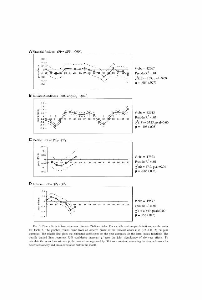
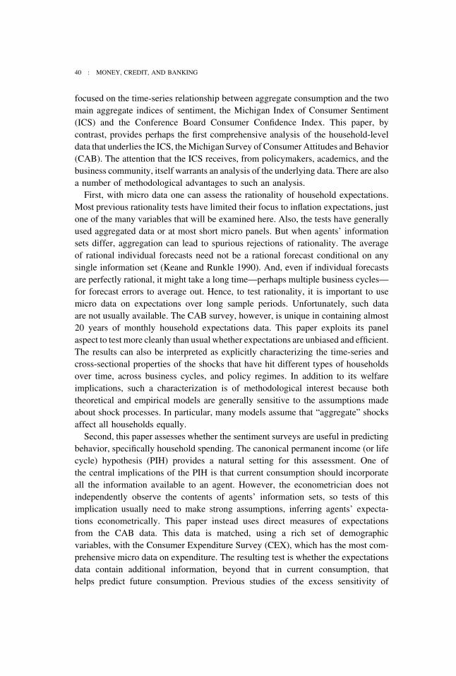
Fig. 3. Time effects in forecast errors: discrete CAB variables. For variable and sample definitions, see the notesfor Table 2. The graphed results come from an ordered probit of the forecast errors ε in {–2,–1,0,1,2} on yeardummies. The middle line gives the estimated coefficients on the year dummies (in the latent index function). Theoutside dashed lines represent 95% confidence intervals. χ2 tests the joint significance of the year effects. Tocalculate the mean forecast error µ, the errors ε are regressed by OLS on a constant, correcting the standard errors forheteroscedasticity and cross-correlation within the month.
56 : MONEY, CREDIT, AND BANKING
probability of its turning out better than expected. In 3 × 3 tables, this requires thatone specify how much worse it is to end up two places (cells) off the diagonal than oneplace off. However, one can avoid taking a stand on this tradeoff by collapsingthe 3 × 3 tables into 2 × 2 tables, by either dropping the middle (0’s) responses orby merging them into one of the other two responses (�1 or �1).23 Nonparametricsign tests can then be used to test whether the probability of falling into the singlenortheast cell significantly differs from the probability of falling into the single south-west cell, a form of bias. Whichever way one handles the middle responses, thesetests (not reported) reject unbiasedness for all four matched pairs of discrete sentimentquestions. In all four cases, “bad” shocks (with financial position, business condi-tions, and income growth turning out worse than expected, and inflation turning outgreater than expected) were more common than “good” shocks over the sampleperiod. However, dropping or merging the middle responses wastes a good dealof information.
Alternatively one can parameterize the errors, most simply by treating their valuesin {�2,�1,0,1,2} as cardinal; i.e., by assuming that being two places off thediagonal is twice as bad as being one place off. Then one can summarize the averageforecast error µ by regressing the errors ε on a constant by OLS. The reportedstandard errors are corrected for the fact that the errors across households in a givenmonth can be correlated by common shocks. In Figure 3, the resulting estimates ofµ for εFP, εBC, and εY are all significantly negative, while the average inflationerror εP is positive. (Recall that for inflation, �1 represents the bad state, the reverseof the other variables.) Again, the realizations are disproportionately biased towardsbeing worse than expected.24
However, as suggested by the nonparametric rationality tests above, one shouldnot conclude from these results that people are generally over-optimistic or over-confident, at all times. One can test for significant time effects in the forecast errorsε, even without cardinalizing them, by using ordered probits. Equation (4) was firstestimated using only the time dummies as independent variables. The resultingcoefficients and 95% confidence intervals are graphed in Figure 3, for the sampleperiods over which each pair of variables is available. For clarity, year dummiesare presented, but the conclusions are the same using the full set of month dummies.For all four discrete forecast errors, the chi-squared tests indicate that the yeardummies are jointly very significant. That is, there is significant variation in house-holds’ forecast errors from year to year. The nonprice errors εFP, εBC, and εY
23. E.g., one could test the rationality of binary variables such as “(a) Will conditions improve orat least stay the same, or (b) will conditions worsen?” This variable would correspond to grouping the0’s with the �1’s.
24. While the reported standard errors control for contemporaneous cross-sectional correlation fromcommon shocks, they do not reflect the fact that the forecast horizons for households interviewed insuccessive months partially overlap, potentially generating serial correlation in the residuals. Since theforecast periods cover six months, this correlation could extend up to five months. To control for this,the regressions were rerun limiting the sample to nonoverlapping forecast periods (e.g., in one regressionusing only CAB interviews in January and July, in another regression using only February and August,etc.). Even though this throws away 5/6 of the data, for εFP and εY the average µ remained significantlynegative for all samples considered (i.e., for all six pairs of months). For εBC and εP the means remainednegative and positive, respectively, and were significant in about half of the nonoverlapping samples.

NICHOLAS S. SOULELES : 57
are most negative throughout the early 1980s and the early 1990s. Consistent withthe results above, it appears that people were negatively surprised by the recessions,repeatedly over their duration.25,26 However, recalling the procyclicality of sentimentin Figures 1 and 2 (in particular, the fact that QFPe is a leading indicator), oneshould not conclude that people altogether fail to foresee the business cycle. Rather,it appears that people understate the amplitude or duration of the cycle, in bothdownturns and upturns. Nonetheless, the pseudo R2’s in Figure 3 suggest that timeeffects explain only a small part of the variation in the forecast errors. The time effectsare more significant and produce a larger R2 for the forecast error for aggregateactivity, εBC, than for the household-specific errors εFP and εY.
Figure 3D records the results for the discrete inflation forecast errors εP. Theyear effects swing from positive to negative. Evidently inflation was higher thanexpected at the end of the 1970s but then people were surprised by how quickly itabated in the early 1980s.27 Figure 4B presents analogous OLS results for thecontinuous, subjective inflation error, εΠsubj. This error also dramatically declinesfrom positive to negative in the early 1980s, and is positive on average over thesample period. Figure 4C shows the objective forecast error εΠobj, which uses asits realization the actual CPI inflation rate Π12 over the next 12 months (as opposedto the respondent-supplied realization QΠr used in Figure 4B, which is not availableafter 1985).28 The errors again decline with the disinflation in the early 1980s.
25. Under basic models of rational expectations, efficiency requires that individual agents’ forecasterrors be independent across time. Even though only one forecast error is available per household, onecan test for serial correlation in the aggregated forecast errors, i.e., in the estimated month dummiesunderlying Figures 3 and 4. There is significant autocorrelation through over 10 months for εFP, εBC,εP, εΠsubj, and εΠobj
6 , and through over 20 months for εΠobj (whose forecast period covers 12 months).However, recall that tests of efficiency on aggregated data are subject to aggregation bias.
26. The overlapping forecast periods described above could generate some autocorrelation throughfive months. But Figure 3 and the results in the previous note show that the autocorrelation in the timeeffects lasts much longer than this. The diagrams and conclusions remain qualitatively the same onlimiting the sample to nonoverlapping periods as above, or on using the full set of month dummiesin Equation (4). Estimating (4) by OLS produces year effects that are similar to those in Figure 3.
27. There is a small discrepancy in the wording of QPe and QPr. QPe asks about prices in general,whereas QPr asks about the prices of goods the household itself buys. This distinction should not mattermuch here. First, the CAB data are representative, so the average price of goods bought should berelatively close to the consumer price level. Second, any discrepancy is unlikely to explain the dramaticshift in forecast errors from positive to negative during the disinflation in the early 1980s. Third, thecontinuous questions QΠe are about aggregate prices and so Figure 4C is not subject to the discrepancy,yet yields a similar pattern. Fourth, Croushore (1998) documents a similar pattern using the aggregatetime series for inflation expectations from the Livingston survey and the Survey of Professional Forecast-ers, where again there is no discrepancy in the wording of the survey questions. Fifth, the results aresimilar on using the regional CPI for the census region in which the household lives, instead of the nationalCPI, or using instead the PCE and GDP deflators. Finally, even though QPe does not specifically mentionthe CPI, both the results of the previous literature and the staff at the Institute for Social Researchsuggest that the CPI is the appropriate benchmark. The ISR surveyors prod respondents for the pricesof “the things people buy,” intending to capture consumer prices, although they deliberately avoid usingjargon like “CPI-U”.
28. The drawbacks to using actual inflation emphasized by Keane and Runkle (1990) do not applyhere. First, unlike the GDP deflator the CPI is not revised. (The seasonal adjustment can be changed,but this is unlikely to be important. To avoid any problem the reported results use the nonseasonallyadjusted CPI. Using the seasonally adjusted CPI instead made extremely little difference.) Second,revisions are a problem only if the revised variable is used as a regressor to test efficiency but was notin agents’ information sets. The efficiency tests here do not use revised variables as regressors.
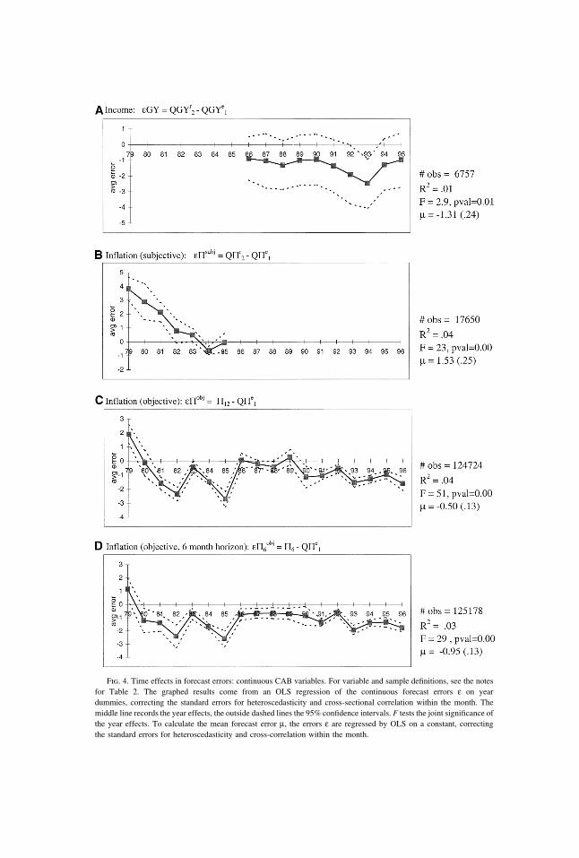
Fig. 4. Time effects in forecast errors: continuous CAB variables. For variable and sample definitions, see the notesfor Table 2. The graphed results come from an OLS regression of the continuous forecast errors ε on yeardummies, correcting the standard errors for heteroscedasticity and cross-sectional correlation within the month. Themiddle line records the year effects, the outside dashed lines the 95% confidence intervals. F tests the joint significance ofthe year effects. To calculate the mean forecast error µ, the errors ε are regressed by OLS on a constant, correctingthe standard errors for heteroscedasticity and cross-correlation within the month.

NICHOLAS S. SOULELES : 59
The magnitude of this decline is both statistically and economically significant, withinflation starting about two percentage points higher than expected in 1979 butfalling to 2.5 percentage points lower than expected by 1982—a large, 4.5 percentagepoint change. More recently, throughout the 1990s households were repeatedlysurprised by the low levels of inflation, by about 1–2 percentage points. Suchnegative errors dominate in the longer sample period, making the overall averageerror µ significantly negative for εΠobj, whereas it was positive for εΠsubj overthe shorter sample period. These results vividly illustrate how sensitive estimatesof bias can be to the sample period, even for long samples. Figure 4D shows theobjective forecast errors εΠobj
6 using instead the CPI inflation rate over only the firstsix months after households’ first interviews (annualized), to see the effectsof the six-month mismatch between expectations and realizations in the other vari-ables. Reassuringly, the results do not much differ from Figure 4C, suggestingthat the mismatch is not driving the conclusions.29 More generally, the results forinflation are robust across different definitions of inflation and its forecasterror.
Figure 4A displays the forecast errors εGY for income growth, which are availableonly in the later part of the sample period. Despite the larger standard errors(reflecting the smaller sample size), the forecast errors still significantly vary overtime. They start declining in 1990, and rebound only after 1993, when incomegrowth was 2.5 percentage points lower than expected. Again, people seem tohave been surprised by the recession, and perhaps also by the weakness of thesubsequent recovery.30,31
As a further check that the six-month timing mismatch is not driving the results,forecast errors with the correct timing can be estimated for each household i. Foreach matched expectational question Qe
1,i, the realization exactly 12 months laterQr
12,i can be estimated from the corresponding realizations Qrj of other households
j with the same characteristics Z that are interviewed 12 months later. The resultingforecast errors ε12 ≡ Qr
12 � Qe1 exhibit very similar means and time effects as those
graphed in Figures 3 and 4A,B. The other conclusions given below also persist,
29. In addition to having similar time-series properties, the cross-sectional properties of εΠobj6 are
similar to those for εΠobj in Table 2 below, both qualitatively and quantitatively. Further, their six-monthdifference does not materially change the Euler equation results for εΠobj below in Table 4.
30. Though part of the reason εGY troughs as late as 1993 might be the small lag in its referenceperiod, discussed above.
31. Again, these conclusions persist on dropping the overlapping forecast periods. The average errorsµ for εΠsubj and εΠ6
obj remain significant in all six nonoverlapping samples. (For εΠobj µ is less significant,but with a 12 month horizon, twice as much of the data (11/12) had to be dropped. Even so εΠobj stillvaries significantly over time, in all the nonoverlapping samples.) For εGY µ remains significant inover half of the nonoverlapping samples. To allow for one month’s delay in the release of the CPI,this analysis was redone dropping 6/7 of the data for εΠobj
6 and 12/13 for εΠobj. The conclusionsare the same. As already noted, the serial correlation in the aggregated inflation errors lasts well overa year.

60 : MONEY, CREDIT, AND BANKING
confirming that the timing mismatch is not a problem.32,33 Further, the consistencyof the results in Figures 3 and 4 suggests that the results in Figure 3 are not drivenby the discreteness of its variables.
In sum, consumer forecasts appear to have been biased. However, it is verydifficult to distinguish whether they were biased ex ante, or just ex post, requiringmany years—perhaps many business cycles—to meet their targets on average. Ineither case, the bias is problematic for empirical studies with short sample periods.In particular, the business cycle and inflation regime induce low-frequency system-atic patterns in average forecast errors.
Turning to the cross-sectional properties of forecast errors, the demographicvariables Z were added to the models of the forecast errors ε using Equation (4),along with the full set of month dummies (but not yet interacting age and incomeby month). Table 2 records the results, starting with ordered probit models ofthe discrete errors in columns (1) to (4). The pseudo R2’s are small, implying that theforecast errors are largely unsystematic, as expected. Nonetheless, according tothe chi-squared statistics the demographic variables are jointly very significant, forall four discrete errors. Hence the forecasts appear to have been inefficient. While itis difficult to interpret individual coefficients in this context, there are some interestingpatterns. As regards financial position in column (1), the errors εFP tend to be morepositive on average for older, higher income, and higher education households,more negative for divorcees and minorities. Since the overall average error µwas negative (Figure 3A), the bias in the forecasts QFPe tends to decrease inmagnitude with age, income, and education.
The pattern of results is roughly similar for business conditions εBC and incomeεY in columns (2) and (3), and often reversed in sign for inflation εP (which hasthe opposite coding) in column (4). Columns (5)–(7) show analogous results forthe continuous income and inflation variables, estimated by OLS. In all cases, thedemographic variables are again jointly quite significant, counter to the requirementof efficiency. They are also economically significant. For instance, in column (7),the inflation forecast error is about 0.4 percentage points larger in magnitude (morenegative) for those without high school education, relative to those with high schooleducation. The error is about 1.0 percentage point larger as real (1982–84 $) house-hold income declines from $50,000 to $10,000, and for minorities and femalesrelative to whites and males.
32. Because ε12 is continuous, the estimation is by OLS. While this changes the magnitude of thetime effects compared to the ordered probit time effects for ε graphed in Figure 3, the differencesare small even quantitatively. Overall, the differences in the time effects for ε12 versus ε are generallycomparable in scope to the differences for εΠobj
6 versus εΠobj graphed in Figures 4C, D. The cross-sectional properties of ε12 are also similar to those for ε in Table 2.
33. The similarity of the results for ε and ε12 also suggests that recall bias is not driving the conclusions,because ε and ε12 are calculated using different realization questions with only partly overlapping referenceperiods. Severe recall bias would imply little overlap between these realization questions. Further, recallbias is unlikely to be correlated with monetary policy, the business cycle, and skill-biased technical change,so is unlikely to explain the results in Figures 3–5. Finally, if the systematic components in the measuredforecast errors simply reflected recall bias, not actual shocks, they should not help predict consumptionchanges below.

TA
BL
E2
Cro
ss-s
ecti
onal
Het
erog
enei
tyin
Fore
cast
Err
ors:
CA
BSu
rvey
s,19
78–9
6
(1)
εFP
�Q
FPr 2
�Q
FPe 1
(2)
εBC
�Q
BC
r 2�
QB
Ce 1
(3)
εY�
QY
r 2�
QY
e 1(4
)εP
�Q
Pr 2
�Q
Pe 1
(5)
εGY
�G
Yr 2
�Q
GY
e 1(6
)εΠ
subj
�Q
Πr 2
�Q
Πe 1
(7)
εΠob
j�
Πr 12
�Q
Πe 1
Coe
ffici
ent
S.E
.C
oeffi
cien
tS.
E.
Coe
ffici
ent
S.E
.C
oeffi
cien
tS.
E.
Coe
ffici
ent
S.E
.C
oeffi
cien
tS.
E.
Coe
ffici
ent
S.E
.
Age
�0.
018
0.00
3*�
0.01
00.
003*
�0.
016
0.00
5*0.
003
0.00
50.
754
0.14
7*�
0.02
90.
050
�0.
037
0.01
3*A
ge2 /1
000.
020
0.00
3*0.
005
0.00
3#0.
018
0.00
5*0.
007
0.00
5�
0.67
50.
142*
0.10
60.
052*
0.07
10.
013*
ln(i
ncom
e)0.
067
0.01
1*�
0.00
70.
011
0.07
10.
019*
�0.
050
0.02
0*�
5.29
10.
705*
�0.
370
0.22
1#0.
539
0.05
3*M
arri
ed�
0.01
60.
041
0.03
70.
041
0.09
70.
065
0.09
00.
069
2.11
12.
106
�0.
226
0.60
9�
0.16
50.
123
Sepa
rate
d�
0.07
40.
026*
0.05
10.
026*
�0.
018
0.04
0�
0.02
70.
043
�1.
167
1.24
0�
0.06
70.
416
0.12
30.
114
Non
whi
te�
0.11
90.
026*
�0.
031
0.02
5�
0.06
50.
041
0.12
80.
043*
�1.
289
1.26
10.
126
0.53
5�
0.81
50.
140*
Fem
ale
0.00
50.
023
�0.
025
0.02
3�
0.00
10.
036
0.14
60.
038*
�1.
360
1.07
51.
032
0.33
8*�
0.97
00.
098*
No
high
�0.
021
0.02
3�
0.02
50.
023
�0.
008
0.03
50.
038
0.03
7�
0.97
01.
169
�0.
337
0.39
1�
0.39
60.
112*
scho
olSo
me
�0.
010
0.01
9�
0.04
30.
019*
�0.
015
0.03
1�
0.08
00.
033*
1.23
40.
816
�0.
051
0.29
70.
269
0.07
3*co
llege
Col
lege
0.05
70.
019*
�0.
032
0.01
9#0.
082
0.03
1*�
0.11
10.
033*
1.30
30.
837
�0.
336
0.25
00.
099
0.06
71
kid
�0.
029
0.02
1�
0.02
30.
021
�0.
081
0.03
5*�
0.00
50.
037
�0.
634
0.96
3�
0.36
10.
308
�0.
152
0.08
6#2
kids
�0.
030
0.02
2�
0.01
80.
022
�0.
007
0.03
7�
0.03
40.
039
0.19
40.
962
0.01
70.
341
�0.
319
0.08
6*3�
kids
�0.
049
0.02
8#�
0.01
40.
027
�0.
047
0.04
6�
0.04
30.
049
�0.
416
1.18
6�
0.30
40.
431
�0.
504
0.12
0*2
adul
ts0.
037
0.03
8�
0.02
90.
038
�0.
105
0.06
1#�
0.00
70.
065
�0.
007
1.94
50.
822
0.55
20.
097
0.10
83�
adul
ts0.
017
0.04
4�
0.02
20.
044
�0.
075
0.07
2�
0.05
40.
076
�1.
093
2.17
31.
271
0.62
4*0.
026
0.12
8M
idw
est
0.01
80.
020
0.05
30.
020*
�0.
023
0.03
3�
0.03
80.
035
0.01
20.
844
�0.
532
0.29
5#0.
116
0.08
1So
uth
0.01
90.
020
0.04
20.
020*
0.01
90.
032
�0.
024
0.03
4�
1.16
70.
860
�0.
215
0.30
60.
001
0.08
1W
est
�0.
043
0.02
2*0.
025
0.02
2�
0.05
50.
036
�0.
081
0.03
8*�
1.57
70.
939#
�0.
531
0.32
8#�
0.23
70.
086*
log
�31
068
�32
366
�11
252
�89
19lik
elih
ood
#ob
s23
798
2377
592
9594
0548
5687
8860
695
Pseu
doR
20.
010.
050.
010.
04R
20.
030.
050.
05χ2
[pva
l]22
8[0
.00]
158
[0.0
0]74
[0.0
0]40
1[0
.00]
F[p
val]
5.52
[0.0
0]9.
51[0
.00]
35.3
[0.0
0]
Not
es:
Thi
sta
ble
anal
yzes
the
syst
emat
icde
mog
raph
icco
mpo
nent
sof
fore
cast
erro
rsε,
usin
gE
quat
ion
(4).
Inco
lum
ns(1
)to
(4),
the
fore
cast
erro
rsar
edi
scre
tean
dth
ees
timat
ion
isby
orde
red
prob
it.Fo
rea
chm
atch
edpa
irof
sent
imen
tqu
estio
ns,Q
e 1re
pres
ents
anex
pect
atio
nfr
oma
hous
ehol
d’s
first
inte
rvie
w,Q
r 2th
eco
rres
pond
ing
real
izat
ion
from
itsse
cond
inte
rvie
w.E
xcep
tfo
rin
flatio
n,Q
��
1re
pres
ents
the
bette
rst
ates
(e.g
.,be
tter
orgo
od),
0th
ein
term
edia
test
ates
,�
1th
ew
orse
stat
es.
Fore
cast
erro
rsar
eth
edi
ffer
ence
betw
een
expe
ctat
ions
and
real
izat
ions
:ε
�(Q
r 2�
Qe 1)
,w
ithva
lues
in{–
2,–1
,0,1
,2}.
Inco
lum
ns(5
)–(7
),th
efo
reca
ster
rors
are
cons
truc
ted
anal
ogou
sly
but
are
cont
inuo
us-v
alue
d;es
timat
ion
isby
OL
S,co
rrec
ting
the
stan
dard
erro
rsfo
rhe
tero
sced
astic
ity.C
oeffi
cien
tson
mon
thdu
mm
ies
are
not
show
n.T
heom
itted
cate
gori
cal
vari
able
sar
e:si
ngle
,whi
te,m
ale
head
,hig
hsc
hool
grad
uate
,no
kids
,one
adul
t,no
rthe
ast.
χ2an
dF
test
the
join
tsi
gnifi
canc
eof
the
dem
ogra
phic
vari
able
s,w
ithp-
valu
esin
the
brac
kets
.In
colu
mns
(1)–
(6)
the
sam
ple
islim
ited
toho
useh
olds
inte
rvie
wed
twic
e.Fu
rthe
r,th
esa
me
pers
on(e
ither
head
orsp
ouse
)m
usth
ave
been
the
resp
onde
ntin
both
inte
rvie
ws.
Inco
lum
n(7
),w
hich
uses
the
actu
alC
PIin
flatio
nra
teΠ
12as
the
real
izat
ion,
the
hous
ehol
dm
ayha
vebe
enin
terv
iew
edon
lyon
ce;
and
ifin
terv
iew
edtw
ice,
the
resp
onde
ntne
edno
tbe
the
sam
epe
rson
inbo
thin
terv
iew
s.#
repr
esen
tssi
gnifi
canc
eat
the
10%
leve
l,*
repr
esen
tssi
gnifi
canc
eat
the
5%le
vel.

62 : MONEY, CREDIT, AND BANKING
Whether one should interpret these results as evidence of “irrationality” is a subtleissue. It could be that young, low income, and low education people have perfectlyrational expectations ex ante, but ex post happened to have received disproportion-ately bad shocks over the sample period. This is consistent with the literature findingincreased inequality over the period, in part due to skill-biased technical change(e.g., Cutler and Katz, 1991, Attanasio and Davis, 1996). But even the ex postinterpretation of the results is problematic for empirical studies that assume that timedummies capture all systematic components of forecast errors. Further, the ineffi-ciency of the forecasts of aggregate variables (QBC, QP, and QΠ) is harder toexplain, and more likely represents ex ante inefficiency. Even if people receivedifferent shocks to their own income and financial position, household-specificshocks should have less effect on their forecasts of aggregate economic activityand prices.
The cross-sectional distribution of forecast errors can change over time. To illus-trate, Figure 5 shows the sample average of the errors in financial position εFP, year-by-year for different demographic groups. Since income and age are the variablesinteracted with time below, the figures contrast the histories of the top and bottomquartiles of the income and age distributions. In Figure 5A for income, the errors arealways more negative for low-income households than for high-income households,though they are more cyclical for the high-income households. One interpretationis that during the expansions high-income households received relatively goodshocks but low-income households continued to receive somewhat negative shockson balance, consistent with ongoing skill-biased technical change. These results gobeyond most of the literature on technical change by implying that the increasedinequality was repeatedly unexpected, year after year, which has additional welfareconsequences. In Figure 5B for age, the errors for young households are bothmore negative and more cyclical than for older households. This suggests that long-run and business cycle shocks disproportionately hit young households.
5. RESULTS: EXCESS SENSITIVITY AND SYSTEMATICHETEROGENEITY IN FORECAST ERRORS
Even if expectations are not fully rational, they might still help forecast spending.To test for excess sensitivity of consumption to sentiment, the sentiment variablesQ were first imputed into the CEX using an OLS regression of Equation (1). Forbrevity, these results are not reported but are available in the working-paper version.34
In this first-step, most of the demographic variables were significant, and jointlythey were very significant. In Table 3, column (1) shows the resulting adjusted R2’sfrom the first-step regressions. More of the level of sentiment is explained than thatof the associated forecast errors (in Table 2), as expected. The dynamic variables
34. The working paper reported the first-step results using ordered probit models for the discretesentiment questions. Those results are qualitatively similar to the OLS results.

NICHOLAS S. SOULELES : 63
Fig. 5. Time effects in forecast errors, by demographic groups: financial position εFP. The figures graph the samplemeans of the error εFP in financial position (See Table 2.), for the bottom and top quarters of the income andage distributions.
in Equation (1), namely the month dummies and their interactions with age andincome, were always significant.35 The “static R2’s” in brackets in column (1) comefrom redoing the estimation without the dynamic variables. For all the household-specific variables (QFPr, QFPe, QYe, and QGYe), the static R2 is well over half
35. To ease the computational demands, the quadratic term in age has been dropped. Preliminaryanalysis suggested that for most sentiment questions the quadratic term did not vary as significantlyacross time.
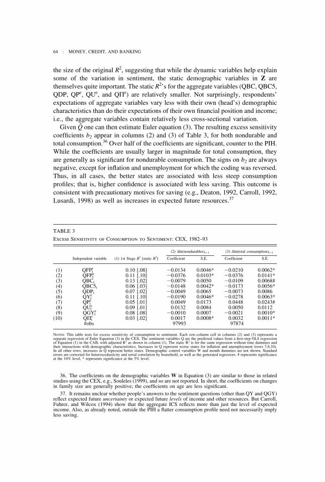
64 : MONEY, CREDIT, AND BANKING
the size of the original R2, suggesting that while the dynamic variables help explainsome of the variation in sentiment, the static demographic variables in Z arethemselves quite important. The static R2’s for the aggregate variables (QBC, QBC5,QDP, QPe, QUe, and QΠe) are relatively smaller. Not surprisingly, respondents’expectations of aggregate variables vary less with their own (head’s) demographiccharacteristics than do their expectations of their own financial position and income;i.e., the aggregate variables contain relatively less cross-sectional variation.
Given Q one can then estimate Euler equation (3). The resulting excess sensitivitycoefficients b2 appear in columns (2) and (3) of Table 3, for both nondurable andtotal consumption.36 Over half of the coefficients are significant, counter to the PIH.While the coefficients are usually larger in magnitude for total consumption, theyare generally as significant for nondurable consumption. The signs on b2 are alwaysnegative, except for inflation and unemployment for which the coding was reversed.Thus, in all cases, the better states are associated with less steep consumptionprofiles; that is, higher confidence is associated with less saving. This outcome isconsistent with precautionary motives for saving (e.g., Deaton, 1992, Carroll, 1992,Lusardi, 1998) as well as increases in expected future resources.37
TABLE 3
Excess Sensitivity of Consumption to Sentiment: CEX, 1982–93
(2) ∆ln(nondurables)t�1 (3) ∆ln(total consumption)t�1
Independent variable (1) 1st Stage R2 [static R2] Coefficient S.E. Coefficient S.E.
(1) QFPrt 0.10 [.08] �0.0134 0.0046* �0.0210 0.0062*
(2) QFPet 0.11 [.10] �0.0376 0.0103* �0.0376 0.0141*
(3) QBCt 0.13 [.02] �0.0079 0.0050 �0.0109 0.0068#(4) QBC5t 0.06 [.03] �0.0148 0.0042* �0.0173 0.0056*(5) QDPt 0.07 [.02] �0.0049 0.0065 �0.0073 0.0086(6) QYe
t 0.11 [.10] �0.0190 0.0046* �0.0278 0.0063*(7) QPe
t 0.05 [.01] 0.0049 0.0173 0.0448 0.0243#(8) QUe
t 0.09 [.01] 0.0132 0.0084 0.0050 0.0112(9) QGYe
t 0.08 [.08] �0.0010 0.0007 �0.0021 0.0010*(10) QΠe
t 0.03 [.02] 0.0017 0.0008* 0.0032 0.0011*#obs 97993 97874
Notes: This table tests for excess sensitivity of consumption to sentiment. Each row-column cell in columns (2) and (3) represents aseparate regression of Euler Equation (3) in the CEX. The sentiment variables Q are the predicted values from a first-step OLS regressionof Equation (1) in the CAB, with adjusted R2 as shown in column (1). The static R2 is for the same regression without time dummies andtheir interactions with demographic characteristics. Increases in Q represent worse states for inflation and unemployment (rows 7,8,10).In all other rows, increases in Q represent better states. Demographic control variables W and month dummies are not shown. Standarderrors are corrected for heteroscedasticity and serial correlation by household, as well as the generated regressors. # represents significanceat the 10% level, * represents significance at the 5% level.
36. The coefficients on the demographic variables W in Equation (3) are similar to those in relatedstudies using the CEX, e.g., Souleles (1999), and so are not reported. In short, the coefficients on changesin family size are generally positive; the coefficients on age are less significant.
37. It remains unclear whether people’s answers to the sentiment questions (other than QY and QGY)reflect expected future uncertainty or expected future levels of income and other resources. But Carroll,Fuhrer, and Wilcox (1994) show that the aggregate ICS reflects more than just the level of expectedincome. Also, as already noted, outside the PIH a flatter consumption profile need not necessarily implyless saving.

NICHOLAS S. SOULELES : 65
Most of the insignificant excess sensitivity coefficients are for questions referringto aggregate variables: QBC, QDP, QPe, and QUe. In part, this is the result of theirhaving less cross-sectional variation, conditional on the time dummies, as evidencedby their smaller first-step static R2’s. Conversely, almost all the household-specificvariables generate significant excess sensitivity.38 Thus, the cross-sectional informa-tion in sentiment appears to help predict future consumption.
There are many possible sources of this excess sensitivity. One possibility isunobserved differences in discount factors and other household fixed effects. Follow-ing Runkle (1991), lagged consumption growth from households’ first interview wasadded to Equation (3) to control for household fixed effects, at the cost of reducedsample size and power. Nonetheless, over half of the significant coefficients fornondurable consumption in Table 3 remain significant, including QFPe, QBC5, andQYe. While QFPr and QΠe become less significant, QPe becomes more significant.39
Hence, heterogeneous discount factors and other fixed effects cannot alone begenerating the estimated excess sensitivity. Further, Hausman tests and autocorrela-tion tests of the residuals produce little evidence for the presence of fixed effects,consistent with the previous literature (Browning and Lusardi 1996).40
Another possible, but understudied, explanation for the results is time-varying,systematic heterogeneity in forecast errors. This is especially likely to be a problemsince both sentiment and forecast errors have just been found to be correlated withthe same household demographic characteristics. These findings suggest that evena long sample period and a full set of time dummies might not be enough to ensureorthogonality of the forecast errors in the residual with the sentiment regressors.Since the forecast errors are likely to be correlated with many regressors of interest,this would be a general problem.
To verify this suggestion directly, estimates of the forecast errors ε were addedto Euler equation (3), for the variables for which there are matching realizationand expectation questions. Table 4 shows the results, after imputing the forecast
38. Even though QFPr does not ask about the future, time-series studies have similarly found thecoincident component of the aggregate ICS index (QFPr �QDP) to be useful in forecasting (e.g.,Throop 1992).
39. These results do not correct the standard errors for the generated sentiment regressors, becausethe Angrist and Krueger (1992) estimator requires that the independent variables in Equation (3)be available in the first-step dataset, but the CAB does not measure consumption growth.
40. Most studies assume that preferences are identical across agents, in which case the time dummiescontrol for the net discount factors [(r-ρ)t]. Omitted fixed effects should lead to positive autocorrelationin the residuals of individual households’ consumption growth. However, in all regressions in Tables 3and 4 the residuals are negatively correlated at both the first and second household lags. The Hausmantest is motivated by the fact that adding lagged consumption growth provides consistency in the presenceof fixed effects, but inefficiency in their absence. In 17 of the 20 Euler equations in Table 3, the Hausmantest fails to find evidence for fixed effects. Also, the three exceptions are all for sentiment questionsregarding aggregate variables (QDP, QP, QΠ), yet it would be surprising if households’ discountfactors were more correlated with aggregate sentiment questions than with household-specific senti-ment questions. (Further, the excess-sensitivity coefficients for two of these exceptions, QDP and QP,are already insignificant in Table 3, before adding lagged consumption growth. Hence their Hausmantest results do not imply that failure to control for fixed effects generated any spurious excess sensitivity.)Similarly, in Table 4, most of the Hausman tests fail to find evidence for fixed effects.

66 : MONEY, CREDIT, AND BANKING
TABLE 4
Excess Sensitivity and Systematic Heterogeneity in Forecast Errors: CEX, 1982–93
(1) ∆ln(nondurables)t�1 (2) ∆ln(total consumption)t�1
Independent variables Coefficient S.E. Coefficient S.E.
(1) QFPet �0.0374 0.0105* �0.0375 0.0142*
εFPt�1( � QFPrt�1 � QFPe
t ) 0.0186 0.0075* 0.0105 0.0101# obs 97993 97874
(2) QBCet �0.0065 0.0089 0.0091 0.0119
εBCt�1( � QBCrt�1 � QBCe
t ) 0.0186 0.0072* 0.0115 0.0100# obs 97993 97874
(3) QYet �0.0031 0.0098 �0.0087 0.0135
εYt�1(QYrt�1 � QYe
t ) 0.0269 0.0158# 0.0255 0.0219# obs 29528 29504
(4) QPet 0.0020 0.0342 0.0318 0.0450
εPt�1( � QPrt�1 � QPe
t ) �0.0124 0.0148 �0.0033 0.0200# obs 29528 29504
(5) QGYet �0.0047 0.0017* �0.0045 0.0023*
εGYt�1( � QGYrt�1 � QGYe
t ) 0.0014 0.0004* 0.0010 0.0005*# obs 30292 30255
(6) QΠet �0.0010 0.0015 �0.0001 0.0020
εΠt�1( � QΠrt�1 � QΠe
t ) �0.0024 0.0013# �0.0035 0.0018*# obs 29528 29504
Notes: This table tests whether the excess sensitivity in Table 3 is due to systematic heterogeneity in forecast errors. See the notes toTable 3. Each row-column cell represents a separate regression of Euler Equation (3) in the CEX. The forecast errors ε � Qr
t�1 � Qet are
first estimated in the CAB using OLS regressions of Equation (4), then imputed in the CEX. Demographic control variables W and monthdummies are not shown. Standard errors are corrected for heteroscedasticity and serial correlation by household, as well as the generatedregressors. # represents significance at the 10% level, * represents significance at the 5% level.
errors into the CEX using Equation (4) (now interacting age and income by month):�
εt�1 ≡ Qrt�1�Qe
t . Despite the time dummies in Equation (3), the coefficients b3 onthe errors ε are often significant. Except for inflation, when they are significant theyare positive: positive innovations in financial position, income, etc., are correlatedwith increases in consumption, as expected. For the inflation questions QP and QΠ,with the opposite coding, the coefficients are negative. But even controlling for theforecast errors, the excess sensitivity regressor b2 remains significantly negative fortwo of the household-specific variables, QFPe and QGYe (in rows (1) and (5)). Thatis, some excess sensitivity persists and so is not due to heterogeneity in forecast errorsalone.41 On the other hand, b2 has become insignificant for the third household-specific variable QYe, as well as for QBCe, QPe, and QΠe. Hence some, though notall, of the excess sensitivity appears to be due to systematic heterogeneity inforecast errors. This suggests the possibility that previous excess sensitivity testsmight have made spurious inferences.
41. Of course, it is possible that even the remaining excess sensitivity is spurious, due to othersystematic heterogeneity in forecast errors that matters for consumption but is not controlled for by theavailable sentiment variables (or due to other sources of mispecification, such as intertemporal nonsepara-bility or liquidity constraints). However, shocks to income, financial position, aggregate economic activityand prices must be among the most important sources of innovations to consumption. Further, asalready noted, under the null hypothesis that forecast errors are classical, they should be orthogonal toother factors in agents’ information sets, including discount rates. Hence the effect in Table 4 of addingforecast errors to the Euler equation cannot be due to such factors.
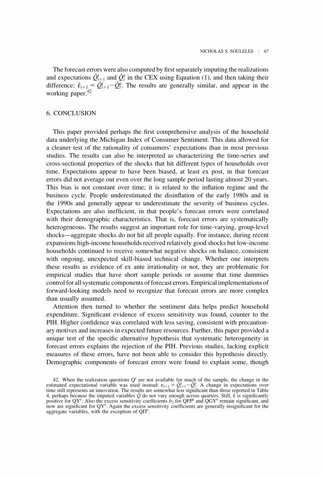
NICHOLAS S. SOULELES : 67
The forecast errors were also computed by first separately imputing the realizationsand expectations Qr
t�1 and Qet in the CEX using Equation (1), and then taking their
difference: εt�1 � Qrt�1�Qe
t . The results are generally similar, and appear in theworking paper.42
6. CONCLUSION
This paper provided perhaps the first comprehensive analysis of the householddata underlying the Michigan Index of Consumer Sentiment. This data allowed fora cleaner test of the rationality of consumers’ expectations than in most previousstudies. The results can also be interpreted as characterizing the time-series andcross-sectional properties of the shocks that hit different types of households overtime. Expectations appear to have been biased, at least ex post, in that forecasterrors did not average out even over the long sample period lasting almost 20 years.This bias is not constant over time; it is related to the inflation regime and thebusiness cycle. People underestimated the disinflation of the early 1980s and inthe 1990s and generally appear to underestimate the severity of business cycles.Expectations are also inefficient, in that people’s forecast errors were correlatedwith their demographic characteristics. That is, forecast errors are systematicallyheterogeneous. The results suggest an important role for time-varying, group-levelshocks—aggregate shocks do not hit all people equally. For instance, during recentexpansions high-income households received relatively good shocks but low-incomehouseholds continued to receive somewhat negative shocks on balance, consistentwith ongoing, unexpected skill-biased technical change. Whether one interpretsthese results as evidence of ex ante irrationality or not, they are problematic forempirical studies that have short sample periods or assume that time dummiescontrol for all systematic components of forecast errors. Empirical implementations offorward-looking models need to recognize that forecast errors are more complexthan usually assumed.
Attention then turned to whether the sentiment data helps predict householdexpenditure. Significant evidence of excess sensitivity was found, counter to thePIH. Higher confidence was correlated with less saving, consistent with precaution-ary motives and increases in expected future resources. Further, this paper provided aunique test of the specific alternative hypothesis that systematic heterogeneity inforecast errors explains the rejection of the PIH. Previous studies, lacking explicitmeasures of these errors, have not been able to consider this hypothesis directly.Demographic components of forecast errors were found to explain some, though
42. When the realization questions Qr are not available for much of the sample, the change in theestimated expectational variable was used instead: εt�1 � Qe
t�1�Qet . A change in expectations over
time still represents an innovation. The results are somewhat less significant than those reported in Table4, perhaps because the imputed variables Q do not vary enough across quarters. Still, ε is significantlypositive for QYe. Also the excess sensitivity coefficients b2 for QFPe and QGYe remain significant, andnow are significant for QYe. Again the excess sensitivity coefficients are generally insignificant for theaggregate variables, with the exception of QΠe.

68 : MONEY, CREDIT, AND BANKING
not all, of the excess sensitivity. More broadly, because forecast errors are correlatedwith household demographic characteristics, they will be correlated with manyregressors of interest in forward-looking models, suggesting that nonclassical fore-cast errors are in practice a general problem. Finally, the cross-sectional variationin sentiment, net of time dummies, was itself found to be informative. This isinformation lost in the aggregated ICS time series for sentiment; nor is it con-tained in other macro variables used in forecasting. Of the Michigan survey questions,those asking specifically about the household, rather than the aggregate economy,were generally found to contain the most useful cross-sectional information.
This analysis can be extended in a number of ways. First, given the significanceof the cross-sectional distribution of sentiment, new sentiment time-series mightbe created to better incorporate this distribution, for instance by taking weightedaverages of sentiment across households.43 Second, one can similarly examine manyother economic decisions in addition to spending for which expectations matter,such as portfolio choice. Cross-sectional data is especially well suited to studyingthe effects of one-time events, like the 1987 stock market crash. Third, durablespurchases might be modeled more explicitly, taking into account their discreteness.
APPENDIX A: THE DATA
A.1 The CAB Survey
The additional sentiment questions, not part of the aggregate ICS index, includethe following. The allowed responses are in brackets (underlining in original).
QBCr. Would you say that at the present time business conditions are better orworse than they were a year ago? [better now, about same, worse now]
QBCe. And how about a year from now, do you expect that in the country as awhole, business conditions will be better or worse than they are at present, or justabout the same? [better a year from now, about same, worse a year from now]
QYr. During the last year or two, would you say that your (family) income wentup more than prices, went up about the same as prices, or went up less than prices?[more, same, less]
QYe. During the next year or two, do you expect that your (family) income willgo up more than prices will go up, about the same, or less than prices will go up?[more, same, less]
QPr. During the last 12 months, have prices of the things you buy remainedunchanged, or have they gone up, or have they gone down? [gone up, remained un-changed, gone down]
QPe. During the next 12 months, do you think that prices in general will go up,or down, or stay where they are now? [go up, will not go up, go down]
43. The weights could reflect e.g., the scale of spending by different groups of people, or the sensitivityof their spending to their sentiment.

NICHOLAS S. SOULELES : 69
QUe. How about people out of work during the coming 12 months—do you thinkthat there will be more unemployment than now, about the same, or less? [more,about same, less]
QGYr. [The growth rate is computed from changes in the level of income takenfrom the following question:] Now, thinking about your (family’s) total income fromall sources (including your job), how much did you (your family) receive in [theprevious calendar year]?
QGYe. By what percent do you expect your (family) income to (increase/decrease)during the next 12 months?
QΠr. By about what percent do you think prices have gone (up/down) on theaverage, during the last 12 months?
QΠe. By about what percent do you expect prices to go (up/down) on the average,during the next 12 months?
Other answers such as “Don’t Know” are also allowed, but are not used here.When the answers to QΠ and QGY were topcoded, they were not used.
For CAB interviews that took place in more than one installment, if these install-ments spanned two different calendar months, the second month is used to date theobservation. If any demographic variable used in a regression is missing, topcoded, orflagged (e.g., Don’t Know), the observation is not used. For the demographicvariables Z, when the continuous measure of total household income was missing,the midpoint of the bracketed income variable was used instead. (But the bracketedvariable is not used in computing the growth rate of income.) The reference periodfor realized income (used in computing the growth rate QGYr) is the previouscalendar year, whereas for the CEX it is the past 12 months. For consistency, CABincome was deflated using the CPI (1982-84 $) for the past 12 months. Since theoriginal CAB income variable is constrained to be positive, for consistency totalincome in the CEX was used only when positive and not flagged. Sample selectionis discussed in the text.
A.2 The CEX Survey
In aggregating individual expenditures, if any component of total consumption ornondurable consumption was topcoded or missing its cost, the whole consumptiongroup was set to missing. If any component was missing its date or dated beforethe reference period, the group was dropped for all interviews for the household atissue. A large number of expenditures are dated in the month of the interview.Following the recommendation of the staff at the BLS, for consistency such expendi-tures were accrued to the following reference period.
In addition to the sample restrictions in the text, an observation is dropped if theage of the head increases by more than one year, or decreases, on moving intothe next quarter. An observation is also dropped if the age of any other memberchanges in this way and thereby results in the member’s switching between beinga kid (less than 16 years old) and an adult (at least 16). If any variable used in aregression is missing, the observation is not used. Other sample restrictions aredescribed in the text.

70 : MONEY, CREDIT, AND BANKING
LITERATURE CITED
Acemoglu, Daron, and Andrew Scott (1994). “Consumer Confidence and Rational Expecta-tions: Are Agents’ Beliefs Consistent with the Theory?” Economic Journal 104, 1–19.
Alessie, Rob, and Annamaria Lusardi (1997). “Saving and Income Smoothing: Evidencefrom Panel Data.” European Economic Review 41, 1251–1279.
Angrist, Joshua, and Alan B. Krueger (1992). “The Effect of Age at School Entry onEducational Attainment: An Application of Instrumental Variables with Moments fromTwo Samples.” Journal of the American Statistical Association 87, 328–336.
Attanasio, Orazio P., and Steven J. Davis (1996). “Relative Wage Movements and theDistribution of Consumption.” Journal of Political Economy 104, 1227–1262.
Attanasio, Orazio P., and Guglielmo Weber (1995). “Is Consumption Growth Consistent withIntertemporal Optimization? Evidence from the Consumer Expenditure Survey.” Journalof Political Economy 95, 1121–1157.
Batchelor, Roy(1986). “Quantitativev. Qualitative Measuresof InflationExpectations.” OxfordBulletin of Economic and Statistics 48, 99–120.
Batchelor, Roy, and Lars Jonung (1989). “Cross-Sectional Evidence on the Rationality ofthe Mean and Variance of Inflation Expectations.” In Understanding Economic Behavior,edited by Klaus G. Grunert, pp. 93–105. Boston: Kluwer Press.
Browning, Martin, and Annamaria Lusardi (1996). “Household Saving: Micro Theories andMicro Facts.” Journal of Economic Literature 34, 1797–1855.
Burch, Susan W., and Stephen E. Gordon (1985). “The Problem of Inference in ConsumerSurveys.” Federal Reserve Board of Governors working paper.
Carroll, Christopher D. (1992). “The Buffer-Stock Theory of Saving: Some MacroeconomicEvidence.” Brookings Papers on Economic Activity 2, 61–156.
Carroll, Christopher D., Karen E. Dynan, and Spencer D. Krane (1996). “Balance Sheetsand Precautionary Saving.” Federal Reserve Board of Governors working paper, January.
Carroll, Christopher D., Jeffrey C. Fuhrer, and David W. Wilcox (1994). “Does ConsumerSentiment Forecast Household Spending? If So, Why?” American Economic Review 84,1397–1408.
Chamberlain, Gary (1984). “Panel Data.” In Handbook of Econometrics, edited by ZviGriliches and Michael D. Intriligator, pp. 1248–1318. Amsterdam: North-Holland.
Croushore, Dean (1998). “Evaluating Inflation Forecasts.” Federal Reserve Bank of Philadel-phia working paper.
Cutler, David M., and Lawrence F. Katz (1991). “Macroeconomic Performance and theDisadvantaged.” Brookings Papers on Economic Activity 1–61.
Das, Marcel, Jeff Dominitz, and Arthur van Soest (1999). “Comparing Predictions andOutcomes: Theory and Application to Income Changes.” Journal of the American StatisticalAssociation 94, 75–85.
Das, Marcel, and Arthur van Soest (1999). “A Panel Data Model for Subjective Informationon Household Income Growth.” Journal of Economic Behavior and Organization 40,409–426.
Deaton, Angus (1992). Understanding Consumption. Oxford, UK: Oxford University Press.
Dominitz, Jeff (1998). “Earnings Expectations, Revisions, and Realications.” Review of Eco-nomics and Statistics 82, 374–388.

NICHOLAS S. SOULELES : 71
Dynan, Karen E. (1993). “How Prudent Are Consumers?” Journal of Political Economy, 101,1104–1113.
Flavin, Marjorie (1991). “The Joint Consumption/Assets Demand Decision: A Case Studyin Robust Estimation.” NBER Working Paper No. 3802.
Friend, Irwin, and F. Gerard Adams (1964). “The Predictive Ability of Consumer Attitudes,Stock Prices, and Non-Attitudinal Variables.” Journal of the American Statistical Associa-tion 59, 987–1005.
Gramlich, Edward M. (1983). “Models of Inflation Expectations Formation.” Journal ofMoney, Credit, and Banking 15, 155–173.
Hall, Robert E., and Frederic S. Mishkin (1982). “The Sensitivity of Consumption to TransitoryIncome: Estimates from Panel Data on Households.” Econometrica 50, 461–482.
Jappelli, Tullio, Jorn-Steffen Pischke, and Nicholas S. Souleles (1998). “Testing for LiquidityConstraints in Euler Equations with Complementary Data Sources.” The Review of Econom-ics and Statistics 80, 251–262.
Jappelli, Tullio, and Luigi Pistaferri (2000). “Using Subjective Income Expectations to Testfor Excess Sensitivity of Consumption to Predicted Income Growth.” European EconomicReview 44, 337–358.
Keane, Michael P., and David E. Runkle (1990). “Testing the Rationality of Price Forecasts:New Evidence from Panel Data.” American Economic Review 80, 714–735.
Ludvigson, Sydney C. (1996). “Consumer Sentiment and Household Expenditure: Reevaluat-ing the Forecasting Equations.” Federal Reserve Bank of New York working paper.
Lusardi, Annamaria (1996). “Permanent Income, Current Income and Consumption: Evidencefrom Two Panel Data Sets.” Journal of Business and Economic Statistics 14, 81–90.
Lusardi,Annamaria (1998). “On the Importance of thePrecautionary SavingMotive.”AmericanEconomic Review 88, 449–453.
Maddala, G.S., Raymond P.H. Fishe, and Kajal Lahiri (1983). “A Time Series Analysis ofPopular Expectations Data.” In Applied Time Series Analysis of Economic Data, editedby Arnold Zellner, pp. 278–290. Washington, DC: U.S. Department of Commerce.
Manski, Charles F. (1990). “The Use of Intentions Data to Predict Behavior: A Best-CaseAnalysis.” Journal of the American Statistical Association 85, 934–940.
Mariger, Randall P., and Kathryn Shaw (1993). “Unanticipated Aggregate Disturbances andTests of the Life-Cycle Consumption Model Using Panel Data.” The Review of Economicsand Statistics 75, 48–56.
McNeil, John (1974). “Federal Programs to Measure Consumer Purchase Expectations,1946–1973: A Post-Mortem.” Journal of Consumer Research 1, 1–10.
Nicholson, Sean, and Nicholas S. Souleles (2002a). “Physician Income Prediction Errors:Sources and Implications for Behavior.” University of Pennsylvania working paper.
Nicholson, Sean, and Nicholas S. Souleles (2002b). “Physician Income Expectations andSpecialty Choice.” University of Pennsylvania working paper.
Runkle, David E. (1991). “Liquidity Constraints and the Permanent-income Hypothesis.”Journal of Monetary Economics 27, 73–98.
Shapiro, Matthew D., and Joel Slemrod (1995). “Consumer Response to the Timing ofIncome: Evidence from a Change in Tax Withholding.” American Economic Review 85,274–283.
Souleles, Nicholas S. (1999). “The Response of Household Consumption to Income TaxRefunds.” American Economic Review 89, 947–958.
Souleles, Nicholas S. (2001). “Household Securities Purchases, Transactions Costs, andHedging Motives.” University of Pennsylvania working paper.

72 : MONEY, CREDIT, AND BANKING
Thomas, Lloyd B. Jr. (1999). “Survey Measures of Expected U.S. Inflation.” Journal ofEconomic Perspectives 13, 125–144.
Throop, Adrien W. (1992). “Consumer Sentiment: Its Causes and Effects.” Federal ReserveBank of San Francisco. Economic Review 0, 35–59.
Zeldes, Stephen P. (1989). “Consumption and Liquidity Constraints: An Empirical Investiga-tion.” Journal of Political Economy 97, 305–346.