First Course in Algorithms through Puzzles

Ryuhei Uehara

Introduction

This book is an introduction to algorithms. What is an algorithm? In short,“algorithm” means “a way of solving a problem.” When people encounter a prob-lem, the approach to solving it depends on who is solving it, and then the efficiencyvaries accordingly. Lately, mobile devices have become quite smarter, planning yourroute when you provide your destination, and running an application when you talkto it. Inside this tiny device, there exists a computer that is smarter than the oldlarge-scale computers, and it runs some neat algorithms to solve your problems.Smart algorithms use clever tricks to reduce computational time and the amountof memory needed. Paul Erdos(1913–

1996):

He was one of the

most productive

mathematicians of

the 20th century,

and wrote more than

1400 journal papers

with more than 500

collaborators. Erdo

numbers are a part

of the folklore of

mathematicians that

indicate the distance

between themselves

and Erdos. Erdos

himself has Erdos

number 0, and his

coauthors have Erdos

number 1. For ex-

ample, the author

has Erdos number

2 because he has

collaborated with a

mathematician who

has Erdos number 1.

One may think that “from the viewpoint of the progress of hardware devices,is an improvement such as this insignificant?” However, you would be wrong. Forexample, take integer programming. Without going into details, it is a generalframework to solve mathematical optimization programs, and many realistic prob-lems can be solved using this model. The running time of programs for solvinginteger programming has been improved 10,000,000,000 times over the last twodecades.1 Surprisingly, the contribution of hardware is 2000 times, and the contri-bution of software, that is, the algorithm, is 475000 times. It is not easy to see, but“the improvement of the way of solving” has been much more effective than “thedevelopment of hardware.”

In this book, the author introduces and explain the basic algorithms and theiranalytical methods for undergraduate students in the Faculty of Information Sci-ence. This book starts with the basic models, and no prerequisite knowledge isrequired. All algorithms and methods in this book are well known and frequentlyused in real computing. This book aims to be self-contained; thus, it is not only atextbook, but also allows you to learn by yourself, or use as a reference book for be-ginners. On the other hand, the author provides some smart tips for non-beginnerreaders.

Exercise. Exercises appear in the text, and are not collected at the end of sections.If you find an exercise when you read this book, the author would like to ask youto take a break, tackle the exercise, and check the answer and comments. For everyexercise, an answer and comments are given in this book.

Each exercise is marked with marks and those with many cups are moredifficult than those with fewer ones. They say that “a mathematician is a machinefor turning coffee into theorems” (this quotation is often attributed to Paul Erdos,however, he ascribed it to Alfred Renyi). In this regard, the author hopes you willenjoy them with cups of coffee.

1R. Bixby, Z. Gu, and Ed Rothberg, “Presolve for Linear and Mixed-Integer Programming,”RAMP Symposium, 2012, Japan.

3

4 INTRODUCTION

Exercises are provided in various ways in your textbooks and reference books.In this book, all solutions for exercises are given. This is rather rare. Actually,this is not that easy from the author’s viewpoint. Some textbooks seem to bemissing the answers because of the authors’ laziness. Even if the author considersa problem “trivial,” it is not necessarily the case for readers, and beginners tendto fail to follow in such “small” steps. Moreover, although it seems trivial at aglance, difficulties may start to appear when we try to solve some problems. Forboth readers and authors, it is tragic that beginners fail to learn because of authors’prejudgments.

Even if it seems easy to solve a problem, solving it by yourself enables you tolearn many more things than you expect. The author is hoping you will try totackle the exercises by yourselves. If you have no time to solve them, The authorstrongly recommends to check their solutions carefully before proceeding to thenext topic.

Analyses and Proofs. In this book, the author provides details of the proofsand the analyses of algorithms. Some unfamiliar readers could find some of themathematical descriptions difficult. However, they are not beyond the range ofhigh school mathematics, although some readers may hate “mathematical induc-tion,” “exponential functions,” or “logarithmic functions.” Although the authorbelieves that ordinary high school students should be able to follow the main ideasof algorithms and the pleasure they bring, you may not lie down on your couch tofollow the analyses and proofs. However, the author wants to emphasize that thereexists beauty you cannot taste without such understanding. The reason why theauthor does not omit these “tough” parts is that the author would like to inviteyou to appreciate this deep beauty beyond the obstacles you will encounter. Eachequation is described in detail, and it is not as hard once you indeed try to follow.

Algorithms are fun. Useful algorithms provide a pleasant feeling much the sameas well-designed puzzles. In this book, the author has included some famous realpuzzles to describe the algorithms. They are quite suitable for explaining the basictechniques of algorithms, which also show us how to solve these puzzles. Throughlearning algorithms, the author hopes you will enjoy acquiring knowledge in such apleasant way.

XX, YY, 2016.Ryuhei Uehara

Contents

Introduction 3

Chapter 1. Preliminaries 11. Machine models 22. Efficiency of algorithm 93. Data structures 114. The big-O notation and related notations 215. Polynomial, exponential, and logarithmic functions 256. Graph 32

Chapter 2. Recursive call 371. Tower of Hanoi 382. Fibonacci numbers 433. Divide-and-conquer and dynamic programming 48

Chapter 3. Algorithms for Searching and Sorting 491. Searching 502. Hashing 563. Sorting 58

Chapter 4. Searching on graphs 771. Problems on graphs 782. Reachability: depth-first search on graphs 793. Shortest paths: breadth-first search on graphs 854. Lowest cost paths: searching on graphs using Dijkstra’s algorithm 89

Chapter 5. Backtracking 971. The eight queen puzzle 982. Knight’s tour 104

Chapter 6. Randomized Algorithms 1131. Random numbers 1142. Shuffling problem 1153. Coupon collector’s problem 119

Chapter 7. References 1231. For beginners 1232. For intermediates 1233. For experts 124

Chapter 8. Answers to exercises 125

5

6 CONTENTS

Conclusion 149

Reference 150

Index 151

CHAPTER 1

Preliminaries

bababababababababababababababab

In this chapter, we learn about (1) machine models, (2) how to measure theefficiency of algorithms, (3) data structures, (4) notations for the analysis ofalgorithms, (5) functions, and (6) graph theory. All of these are very basic,and we cannot omit any of them when learning about/designing/analyzingalgorithms. However, “basic” does not necessarily mean “easy” or “trivial.”If you are unable to understand the principle when you read the text forthe first time, you do not need to be overly worried. You can revise it againwhen you learn concrete algorithms later. Some notions may require someconcrete examples to ensure proper understanding. The contents of thissection are basic tools for understanding algorithms. Although we need toknow which tools we have available, we do not have to grasp all the detailedfunctions of these tools at first. It is not too late to only grasp the principlesand usefulness of the tools when you use them.

What you will learn: • Machine models (Turing machine model, RAM model,

other models)• Efficiency of algorithms• Data structures (array, queue, stack)• Big-O notation• Polynomial, exponential, logarithmic, harmonic functions• Basic graph theory

1

2 1. PRELIMINARIES

1. Machine models

An Algorithm is a method for solving a given problem. Representing howto solve a problem requires you to define basic operations precisely. That is, analgorithm is a sequence of basic operations of some machine model you assume.First, we introduce representative machine models: The Turing machine model,RAM model, and the other models. When you adopt a simple machine model,it is easy to consider the computational power of the model. However, becauseit has poor or restricted operations, it is hard to design/develop some algorithms.On the other hand, if you use a more abstract machine model, even though it iseasier to describe an algorithm, you may face a gap between the algorithm and realcomputers when you implement it. In order to make a sense of balance, it is a goodidea to review some different machine models. We have to mind the machine modelwhen we estimate and/or evaluate the efficiency of an algorithm. Sometimes theefficiency differs depending on the machine model that is assumed.Natural number:

Our natural num-

bers start from 0,

not 1, in the area

of information sci-

ence. “Nonnegative

integers” start from 1.

It is worth mentioning that, currently, every “computer” is a “digital com-puter,” where all data in it is manipulated in a digital way. That is, all data arerepresented by a sequence consisting of 0 and 1. More precisely, all integers, realnumbers, and even irrational numbers are described by a (finite) sequence of 0 and1 in some way. Each single unit of 0 or 1 is called a bit. For example, a naturalnumber is represented by a binary system. Namely, the data 0, 1, 2, 3, 4, 5, 6, . . . arerepresented in the binary system as 0, 1, 10, 11, 100, 101, 110, . . ..

Exercise 1. Describe the numbers 0, 1, 2, 3, 4, 5, 6, 7, 8, 9, 10, 11, 12,13, 14, 15, 16, 17, 18, 19, 20 in the binary and the hexadecimal systems. In thehexadecimal system, 10, 11, 12, 13, 14, and 15 are described by A, B, C, D, E, andF, respectively. Can you find a relationship between these two systems?

Alan Mathison

Turing(1912-1954):

Turing was a British

mathematician and

computer scientist.

The 1930s were the

times before real

computers, he was the

genius who developed

the notion of a “com-

putation model” that

holds good even in our

day. He was involved

with the birth of

computer, took an

important part in

breaking German

codes during World

War II, and died when

he was only 42 years

old from poisoning by

cyanic acid. He was a

dramatic celebrity in

various ways.

Are there non-digital computers? An ordinary computer is a digital computer based on the binary system. Ina real digital circuit, “1” is distinguished from “0” by voltage. That is, apoint represents “1” if it has a voltage of, say, 5V, and “0” if it has a groundlevel voltage, or 0V. This is not inevitable; historically, there were analogcomputers based on analog circuits, and trinary computers based on the trinarysystem of minus, 0, and plus. However, in the age of the author, all computerswere already digital. Digital circuits are simple, and refrain from making anoise. Moreover, “1” and “0” can be represented by other simple mechanisms,including a paper strip (with and without holes), a magnetic disk (N and Spoles), and an optical cable (with and without light). As a result, non-digitalcomputers have disappeared. 1.1. Turing machine model. A Turing machine is the machine model

introduced by Alan Turing in 1936. The structure is very simple because it is avirtual machine defined to discuss the mechanism of computation mathematically.It consists of four parts as shown in Figure 1; tape, finite control, head, andmotor.

The tape is one sided, that is, it has a left end, but has no right end. One ofthe digits 0, 1, or a blank is written in each cell of the tape. The finite control is in

1. MACHINE MODELS 3

Finite Control

Tape for memory

MotorRead/WriteHead

Figure 1. Turing machine model

the “initial state,” and the head indicates the leftmost cell in the tape. When themachine is turned on, it moves as follows:

(1) Read the letter c on the tape;(2) Following the predetermined rule [movement on the state x with letter c],

• rewrite the letter in the head (or leave it);• move the head to the right/left by one step (or stay there);• change the state from x to y;

(3) If the new state is “halt”, it halts; otherwise, go to step 1.The mechanism is so simple that it seems to be too weak. However, in theory,

every existing computer can be abstracted by this simple model. More precisely, thetypical computer that runs programs from memory is known as a von Neumann-typecomputer, and it is known that the computational power of any von Neumann-typecomputer is the same as that of a Turing machine. (As a real computer has limitedmemory, indeed, we can say that it is weaker than a Turing machine!) This factimplies that any problem solvable by a real computer is also solvable by a Turingmachine (if you do not mind their computation time). Theory of compu-

tation:

The theory of com-

putation is a sci-

ence that investigates

“computation” itself.

When you define a

set of basic opera-

tions, the set of “com-

putable” functions are

determined by the op-

erations. Then the

set of “uncomputable”

functions is well de-

fined. Diagonaliza-

tion is a basic proof

tool in this area, and

it is strongly related

to Godel’s Incomplete-

ness Theorem.

Here we introduce an interesting fact. It is known that there exists a problemthat cannot be solved by any computer.

Theorem 1. There exists no algorithm that can determine whether any givenTuring machine with its input will halt or not. That is, this problem, known as thehalting problem, is theoretically unsolvable.

This is one of the basic theorems in the theory of computation, and it is relatedto deep but interesting topics including diagonalization and Godel’s IncompletenessTheorem. However, we mention this as an interesting fact only because these topicsare not the target of this book (see the references). As a corollary, you cannot designa universal debugger that determines whether any program will halt or not. Notethat we consider the general case, i.e., “any given program.” In other words, wemay be able to design an almost universal debugger that solves the halting problemfor many cases, but not all cases.

1.2. RAM model. The Turing machine is a theoretical and virtual machinemodel, and it is useful when we discuss the theoretical limit of computational power.However, it is too restricted or too weak to consider algorithms on it. For example,it does not have basic mathematical operations such as addition and subtraction.Therefore we usually use a RAM (Random Access Machine) model when we

4 1. PRELIMINARIES

Finite Control

Program Couner: PC

Address Data

0000 00000000 00010000 00100000 00110000 0100

1111 11101111 1111

0101 01010000 00001111 11111100 11001100 0011

0000 11111111 0000

Registers

Word

Figure 2. RAM model

Finite Control

Program Counter: PC

Address Data

0000 00000000 00010000 00100000 00110000 0100

1111 11101111 1111

0101 01010000 00001111 11111100 11001100 0011

0000 11111111 0000

Registers

n words

log n bitslog n bits

Figure 3. Relationships among memory size, address, and wordsize of the RAM model. Let us assume that the memory can storen data. In this case, to indicate all the data, log n bits are required.Therefore, it is convenient when a word consists of log n bits. Thatis, a “k bit CPU” usually uses k bits as one word, which meansthat its memory can store 2k words.

discuss practical algorithms. A RAM model consists of finite control, which cor-responds to the CPU (Central Processing Unit), and memory (see Figure 2).Here we describe the details of these two elements.

Memory. Real computers keep their data in the cache in the CPU, memory,and external memory such as a hard disk drive or DVD. Such storage is modeledby memory in the RAM model. Each memory unit stores a word. Data exchangebetween finite control and memory occurs as one word per unit time. Finite controluses an address of a word to specify it. For example, finite control reads a wordfrom the memory of address 0, and writes it into the memory of address 100.

Usually, in a CPU, the number of bits in a word is the same as the number ofbits of the address in the memory (Figure 3). This is because each address itselfcan be dealt with as data. We sometimes say that your PC contains a 64-bit CPU.This number indicates the size of a word and the size of an address. For example,in a 64-bit CPU, one word consists of 64 bits, and one address can be represented

1. MACHINE MODELS 5

from 00 . . . 0︸ ︷︷ ︸64

to 11 . . . 1︸ ︷︷ ︸64

, which indicates one of 264 ≈ 1.8×1019 different data. That

is, when we refer to a RAM model with a 64-bit CPU, it refers to a word with 64bits on each clock, and its memory can store 264 words in total.

Finite control. The finite control unit reads the word in a memory, applies anoperation to the word, and writes the resulting word to the memory again (at thesame or different address at which the original word was stored). A computation isthe repetition of this sequence. We focus on more details relating to real CPUs. ACPU has some special memory units that consist of one program counter(PC),and several registers. When a computer is turned on, the contents of the PC andregisters are initialized by 0. Then the CPU repeats the following operations:

(1) It reads the content X at the address PC to a register.(2) It applies an operation Y according to the value of X.(3) It increments the value of PC by 1.

The basic principle of any computer is described by these three steps. That is, theCPU reads the memory, applies a basic operation to the data, and proceeds to thenext memory step by step. Typically, X is a word consisting of 64 bits. Therefore,we have 264 different patterns. For each of these many patterns, some operationY corresponds to X, which is designed on the CPU. If the CPU is available onthe market, the operations are standardized and published by the manufacturer.(Incidentally, some geeks may remember coding rules in the period of 8-bit CPUs,which only has 28 = 256 different patterns!) Usually, the basic operations on theRAM model can be classified into three groups as follows.

Substitution: For a given address, there is data at the address. This oper-ation gives and takes between the data and a register. For example, whendata at address A is written into a memory at address B, the CPU firstreads the data at address A into a register, and next writes the data in theregister into the memory at address B. Similar substitution operations areapplied when the CPU has to clear some data at address A by replacingit with zero.

Calculation: This operation performs a calculation between two data val-ues, and puts the result into a register. The two data values come froma register or memory cell. Typically, the CPU reads data from a memorycell, applies some calculation (e.g., addition) to the data and some regis-ter, and writes the resulting data into another register. Although possiblecalculations differ according to the CPU, some simple mathematical op-erations can be performed.

Comparison and branch: This operation overwrites the PC if a registersatisfies some condition. Typically, it overwrites the PC if the value ofa specified register is zero. If the condition is not satisfied, the value ofPC is not changed, and hence the next operation will be performed in thenext step. On the other hand, if the condition is satisfied, the value ofthe PC is changed. In this case, the CPU changes the “next address” tobe read, that is, the CPU can jump to an address “far” from the currentaddress. This mechanism allows us to use “random access memory.”

In the early years, CPU allowed very limited operations. Interestingly, this wassufficient in a sense. That is, theoretically, the following theorem is known.

6 1. PRELIMINARIES

Theorem 2. We can compute any function if we have the following set ofoperations: (1) increase the value of a register by one, (2) decrease the value of aregister by one, and (3) compare the value of a register with zero, and branch if itis zero.

Theorem 2 says that we can compute any function if we can design some reason-able algorithm for the function. In other words, the power of a computer essentiallydoes not change regardless of the computational mechanism you use. Nevertheless,the computational model is important. If you use the machine model with the setof operations in Theorem 2, creating a program is quite difficult. You may needto write a program to perform the addition of two integers at the first step. Thus,many advanced operations are prepared as a basic set of operations in recent high-performance CPUs. Although, it seems that there is a big gap between the set ofoperations of the RAM model and real programming languages such as C, Java,Python, and so on. However, any computer program described by some program-ming language can be realized on the RAM model by combining the set of simpleoperations we already have. For example, we can use the notion of a “variable”in most programming languages (see Section 3.1 for the details). It can be realizedas follows on the RAM model:

Example 1. The system assigns that “variable A is located at an address 11111000” when the program starts. Then, substitution to variable A is equivalent tosubstitution to the address 1111 1000. If the program has to read the value invariable A, it accesses the memory with the address 1111 1000.

Using this “variable”, we can realize the usual substitution in a program. Atypical example is as follows.

Example 2. In many programs, “add 1 to some variable A” frequently appears.In this book, we will denote it by

A← A + 1;

When a program based on a RAM model runs this statement, it is processed asfollows (Figure 4): We suppose that the variable A is written at the address 11111000. (Of course, this is an example, which does not correspond to a concrete CPUon the market; rather, this is an example of so-called “assembly language” or“machine language.”)

(1) When it is turned on, the CPU reads the contents at the address PC (=0)in the memory. Then it finds the data “1010 1010” (Figure 4(1)). Fol-lowing the manual of the CPU, the word “1010 1010” means the sequenceof three operations:(a) Read the word W at the next address (PC + 1), and read the data at

address W to the register 1.(b) Read the word W ′ at the address following the next address (PC +2),

and add it to register 1.(c) Write the contents of register 1 to the address following the address

after the next address (PC + 3).(Here the value of PC is incremented by 1.)

(2) The CPU reads the address PC (=1), and obtains the data (=1111 1000).Then it checks the address 1111 1000, and finds the data (=0000 1010).

1. MACHINE MODELS 7

PC=0000 0011

Register 1=0000 1011

PC=0000 0010

Register 1=0000 1011

有限制御部

PC=0000 0001

Register 1=0000 1010

Finite Control

PC=0000 0000Address Data

0000 00000000 00010000 00100000 00110000 0100

1111 1000

1111 11101111 1111

1010 10101111 10000000 00011111 10001010 1010

0000 11111111 0000

Register 1=0000 0000

0000 1010 0000 1011

(1)

(2)

(3)

(4)

(5)

Figure 4. The sequence of statements performed on the RAMmodel: (1) When it is turned on, (2) it reads the contents at address1111 1000 to register 1, (3) it adds 0000 0001 to the contents ofregister 1, (4) it writes the contents in register 1 to the memoryat address 1111 1000, and (5) The contents 0000 1010 at address1111 1000 are replaced by 0000 1011.

Thus, it copies to register 1 (Figure 4(2)). (Here the value of PC isincremented by 1.)

(3) The CPU reads the address PC (=10), and obtains the data (=0000 0001).It adds the data 0000 0001 to register 1, then the contents of register 1 arechanged to 0000 1011 (Figure 4(3)). (Here the value of PC is incrementedby 1.)

(4) The CPU reads the address PC (=11), and obtains the data (=1111 1000)(Figure 4(4)). Thus, it writes the value of the register 1 (=0000 1011) tothe memory at address 1111 1000 (Figure 4(5)). (Here the value of PCis incremented by 1.)

The CPU performs repetitions in a similar way. That is, it increments PC by 1,by reading the data at address PC, and so on.

We note that the PC always indicates “the next address the CPU will read.”Thus, when a program updates the value of PC itself, the program will “jump”to the other address. By this function, we can realize comparison and branching.That is, we can change the behavior of the program.

As already mentioned, each statement of a standard CPU is quite simple andlimited. However, a combination of many simple statements can perform an algo-rithm described by a high-level programming language such as C, Java, Haskell, andProlog. An algorithm written in a high-level programming language is translatedto machine language, which is a sequence of simple statements defined on the CPU,by a compiler of the high-level programming language. On your computer, you Compiler:

We usually “compile”

a computer program,

written in a text file,

into an executable bi-

nary file on a com-

puter. The com-

piler program reads

the computer program

in a text file, and ex-

changes it into the bi-

nary file that is writ-

ten in a sequence of

operations readable by

the computer system.

That is, when we write

a program, the pro-

gram itself is usually

different from the real

program that runs on

your system.

sometimes have an “executable file” with a “source file”; the simple statements arewritten in the executable file, which is readable by your computer, whereas humanreadable statements are written in the source file (in the high-level programminglanguage). In this book, each algorithm is written in a virtual high-level proceduralprogramming language similar to C and Java (in a more natural language style).

8 1. PRELIMINARIES

However, these algorithms can eventually be performed on a simple RAM modelmachine.

Real computers are... In this book, we simplify the model to allow for easy understanding. In somereal computers, the size of a word may differ from the size of an address. More-over, we ignore the details of memory. For example, semiconductor memoryand DVD are “memory,” although we usually distinguish them according totheir price, speed, size, and other properties. 1.3. Other machine models. As seen already, computers use digital data

represented by binary numbers. However, users cannot recognize this at a glance.For example, you can use irrational numbers such as

√2 = 1.4142 . . ., π = 3.141592 . . .,

and trigonometric functions such as sin and cos. You also can compute any functionsuch as eπ, even if you do not know how to compute it. Moreover, your computercan process voice and movie data, which is not numerical data. There exists a biggap between such data and the binary system, and it is not clear as to how tofill this gap. In real computers, representing such complicated data in the simplebinary system is very problematic, as is operating and computing between thesedata in the binary system. It is a challenging problem how to deal with the “com-putational error” resulting from this representation. However, such a numericalcomputation is beyond the scope of this book.

In theoretical computer science, there is a research area known as computa-tional geometry, in which researchers consider how to solve geometric problemson a computer. In this active area, when they consider some algorithms, the repre-sentations of real numbers and the steps required for computing trigonometry arenot their main issues. Therefore, such “trivial” issues are considered in a black box.That is, when they consider the complexity of their algorithms, they assume thefollowing implicitly:

• Each data element has infinite accuracy, and it can be written and readin one step in one memory cell.• Each “basic mathematical function” can be computed in one step with

infinite accuracy.

In other words, they use the abstract machine model on one level higher than theRAM model and Turing machine model. When you implement the algorithmson this machine model onto a real computer, you have to handle computationerrors because any real computer has limited memories. Because the set of basicmathematical functions covers different functions depending on the context, yousometimes have to provide for the implementation of the operations and take careof their execution time.

Lately, new computation frameworks have been introduced and investigated.For example, quantum computer is a computation model based on quantummechanics, and DNA computer is a computation model based on the chemicalreactions of DNA (or string of amino acids). In these models, a computer consists ofdifferent elements and a mechanism to solve some specific problems more efficientlythan ordinary computers.

2. EFFICIENCY OF ALGORITHM 9

In this book, we deal with basic problems on ordinary digital computers. Weadopt the standard RAM model, with each data element being an integer repre-sented in the binary system. Usually, each data element is a natural number, andsometimes it is a negative number, and we do not deal with real numbers and irra-tional numbers. In other words, we do not consider (1) how can we represent data,(2) how can we compute a basic mathematical operation, and (3) computation er-rors that occur during implementation. When we describe an algorithm, we do notsuppose any specific computer language, and use free format to make it easy tounderstand the algorithm itself.

2. Efficiency of algorithm

Even for the same problem, efficiency differs considerably depending on thealgorithms. Of course, efficiency depends on the programming language, codingmethod, and computer system in general. Moreover, the programmer’s skill alsohas influence. However, as mentioned in the Introduction, the choice of an algorithmis quite influential. Especially, the more the amount of data that is given, the morethe difference becomes apparent. Now, what is “the efficiency of a computation”?The answer is the resources required to perform the computation. More precisely,time and space required to compute. These terms are known as time complexityand space complexity in the area of computational complexity. In general, timecomplexity tends to be considered. Time complexity is the number of steps requiredfor a computation, but this depends on the computation model. In this section, wefirst observe how to evaluate the complexity of each machine model, and discussthe general framework.

2.1. Evaluation of algorithms on Turing machine model. It is simpleto evaluate efficiency on the Turing machine model. As seen in section 1.1, theTuring machine is simple, and repeats basic operations. We assume that each basicoperation (reading/writing a letter on the tape, moving the head, and changing itsstate) takes one unit of time. Therefore, for a given input, its time complexity isdefined by the number of times the loop is repeated, and its space complexity ifdefined by the number of checked cells on the tape.

2.2. Evaluation of algorithms on RAM model. In the RAM model, itstime complexity is defined by the number of times the program counter PC isupdated. Here we need to mention two points.

Time to access memory. In the RAM model, one data element in any memorycell can be read/written in one unit of time. This is the reason why this machinemodel is known as “Random Access.” In a Turing machine, if it is necessary to reada data element located far from the current head position, it takes time because themachine has to move the head one by one. On the other hand, this is not the casefor the RAM model machine. When the address of the data is given, the machinecan read or write to the address in one step.

One unit of memory. The RAM model deals with the data in one word in onestep. If it has n words in memory, to access each of them requires log n bits toaccess it uniquely. (If you are not familiar with the function log n, see Section 5 forthe details.) It is reasonable and convenient to assume that one word uses log n bitsin the RAM model, and in fact, real CPUs almost follow this rule. For example,

10 1. PRELIMINARIES

if the CPU in your laptop is said to be a “64-bit CPU”, one word consists of 64bits, and the machine can contain 264 words in its memory; thus we adopt thisdefinition. That is, in our RAM model, “one word” means “log n bits,” where n isthe number of memory cells. Our RAM model can read or write one word in onestep. On the Turing machine, one bit is a unit. Therefore, some algorithms seemto run log n times faster on the RAM model than on the Turing machine model.

Exercise 2. Assume that our RAM model has n words in its memory.Then how many bits are in this memory? In that case, how many different oper-ations can the CPU have? Calculate the number of bits in each RAM model forn = 65536, n = 264, and n = 2k.

2.3. Evaluation of algorithms on other models. When some machinemodel is more abstract than the Turing machine model or RAM model is adopted,you can read/write a real number in a unit time with one unit memory cell, anduse mathematical operations such as power and trigonometry, for which it is notnecessarily clear how to compute them efficiently. In such a model, we measurethe efficiency of an algorithm by the number of “basic operations.” The set ofbasic operations can be changed in the context; however, they usually involve read-ing/writing data, operations on one or two data values, and conditional branches.

When you consider some algorithms on such an abstract model, it is not a goodidea to be unconcerned about what you eliminate from your model to simplify it.For example, by using the idea that you can pack data of any length into a word,you may use a word to represent complex matters to apparently build a “fast”algorithm. However, the algorithm may not run efficiently on a real computer whenyou implement it. Therefore, your choice of the machine model should be reasonableunless it warrants some special case; for example, when you are investigating theproperties of the model itself.

2.4. Computational complexity in the worst case. An algorithm com-putes some output from its input in general. The resources required for the com-putation are known as computational complexity. Usually, we consider twocomputational complexities; time complexity is the number of steps required forthe computation, and space complexity is the number of words (or bits in somecase) required for the computation. (To be precise, it is safe to measure the spacecomplexity in bits, although we sometimes measure this in words to simplify theargument. In this case, we have to concern ourselves with the computation model.)

We have considered the computational complexity of a program running on acomputer for some specific input x. More precisely, we first fix the machine modeland a program that runs on the machine, and then give some input x. Then, its timecomplexity is given by the number of steps, and space complexity is given by thenumber of memory cells. However, such an evaluation is too detailed in general.For example, suppose we want to compare two algorithms A and B. Then, wedecide which machine model to use, and implement the two algorithms on it asprograms, say PA and PB . (Here we distinguish an algorithm from a program. Analgorithm is a description of how to solve a problem, and it is independent from themachine model. In contrast, a program is written in some programming language(such as C, Java, or Python). That is, a program is a description of the algorithm,and depends on the machine and the language.) However, it is not a good idea tocompare them for every input x. Sometimes A runs faster than B, but B may run

3. DATA STRUCTURES 11

faster more often. Thus, we asymptotically compare the behavior of two algorithmsfor “general inputs.” However, it is not easy to capture the behavior for infinitelymany different inputs. Therefore, we measure the computational complexity of analgorithm by the worst case scenario for each length n of input. For each lengthn, we have 2n different inputs from 000 . . . 0 to 111 . . . 1. Then we take the worstcomputation time and the worst computation space for all of the inputs of lengthn. Now, we can define two functions t(n) and s(n) to measure these computationalcomplexities. More precisely, the time complexity t(n) of an algorithm A is definedas follows:

Time complexity of an algorithm A:Let PA be a program that realizes algorithm A. Then, the time complexity t(n)of the algorithm A is defined by the longest computation steps of PA under allpossible inputs x of length n.

Here we note that there is no clear distinction between algorithm A and programPA. In this step, we consider that there are a few gaps between them from theviewpoint of time complexity. We can define the space complexity s(n) of algorithmA in a similar way. Now we can consider the computational complexity of algorithmA. For example, for the time complexities of two algorithms A and B, say tA(n)and tB(n), if we have tA(n) < tB(n) for every n, we say that algorithm A is fasterthan B.

The notion guarantees that it is sufficient to complete the computation evenif we prepare these computational resources for the worst case. In other words,the computation will not fail for any input. Namely, this approach is based onpessimism. From the viewpoint of theoretical computer science, it is the standardapproach because it is required to work well in any of the cases including the worstcase. For example, another possible approach could be “average case” complexity.However, in general, this is much more difficult because we need the distributionof the input to compute the average case complexity. Of course, such a random-ization would proceed well in some cases. Some randomized algorithms and theiranalyses will be discussed in Section 3.4. A typical randomized algorithm is thatknown as quick sort, which is used quite widely in real computers. The quick sortis an interesting example in the sense that it is not only used widely, but also notdifficult to analyze.

3. Data structures

We next turn to the topic of data structures. Data structures continue tobe one of the major active research areas. In theoretical computer science, manyresearchers investigate and develop fine data structures to solve some problemsmore efficiently, smarter, and simpler. However, in this textbook, we only use themost basic and simplest data structure known as an “array.” However, if we restrictourselves to only using arrays, the descriptions of algorithms become unnecessarilycomplicated. Therefore, we will introduce “multi-dimensional array,” “queue,” and“stack” as extensions of the notion of arrays. They can be implemented by usingan array, and we will describe them later.

3.1. Variable. In an ordinary computer, as shown in the RAM model, thereis a series of memory cells. They are organized and each cell consists of a word,which is a collection of bits. Each cell is identified by a distinct address. However,

12 1. PRELIMINARIES

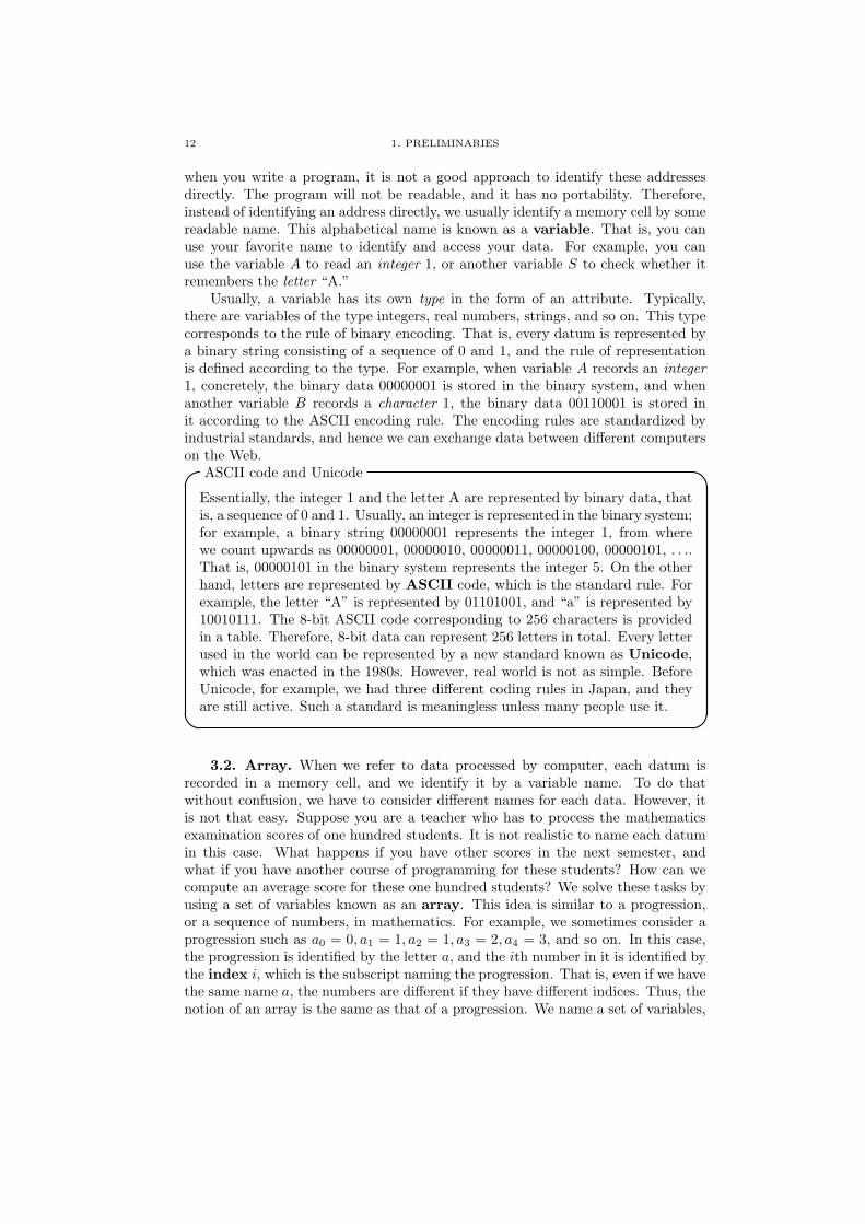
when you write a program, it is not a good approach to identify these addressesdirectly. The program will not be readable, and it has no portability. Therefore,instead of identifying an address directly, we usually identify a memory cell by somereadable name. This alphabetical name is known as a variable. That is, you canuse your favorite name to identify and access your data. For example, you canuse the variable A to read an integer 1, or another variable S to check whether itremembers the letter “A.”

Usually, a variable has its own type in the form of an attribute. Typically,there are variables of the type integers, real numbers, strings, and so on. This typecorresponds to the rule of binary encoding. That is, every datum is represented bya binary string consisting of a sequence of 0 and 1, and the rule of representationis defined according to the type. For example, when variable A records an integer1, concretely, the binary data 00000001 is stored in the binary system, and whenanother variable B records a character 1, the binary data 00110001 is stored init according to the ASCII encoding rule. The encoding rules are standardized byindustrial standards, and hence we can exchange data between different computerson the Web.

ASCII code and Unicode Essentially, the integer 1 and the letter A are represented by binary data, thatis, a sequence of 0 and 1. Usually, an integer is represented in the binary system;for example, a binary string 00000001 represents the integer 1, from wherewe count upwards as 00000001, 00000010, 00000011, 00000100, 00000101, . . ..That is, 00000101 in the binary system represents the integer 5. On the otherhand, letters are represented by ASCII code, which is the standard rule. Forexample, the letter “A” is represented by 01101001, and “a” is represented by10010111. The 8-bit ASCII code corresponding to 256 characters is providedin a table. Therefore, 8-bit data can represent 256 letters in total. Every letterused in the world can be represented by a new standard known as Unicode,which was enacted in the 1980s. However, real world is not as simple. BeforeUnicode, for example, we had three different coding rules in Japan, and theyare still active. Such a standard is meaningless unless many people use it. 3.2. Array. When we refer to data processed by computer, each datum is

recorded in a memory cell, and we identify it by a variable name. To do thatwithout confusion, we have to consider different names for each data. However, itis not that easy. Suppose you are a teacher who has to process the mathematicsexamination scores of one hundred students. It is not realistic to name each datumin this case. What happens if you have other scores in the next semester, andwhat if you have another course of programming for these students? How can wecompute an average score for these one hundred students? We solve these tasks byusing a set of variables known as an array. This idea is similar to a progression,or a sequence of numbers, in mathematics. For example, we sometimes consider aprogression such as a0 = 0, a1 = 1, a2 = 1, a3 = 2, a4 = 3, and so on. In this case,the progression is identified by the letter a, and the ith number in it is identified bythe index i, which is the subscript naming the progression. That is, even if we havethe same name a, the numbers are different if they have different indices. Thus, thenotion of an array is the same as that of a progression. We name a set of variables,

3. DATA STRUCTURES 13

and identify each of them by its index. In a progression, we usually write a1, a2,but we denote an array as a[1], a[2]. That is, a[1] is the 1st element of array a,and a[2] is the second element of array a. In a real computer (or even in the RAMmodel), the realization of an array is simple; the computer provides a sequenceof memory cells, and names the area by the array name, with a[i] indicating theith element of this memory area. For example, we assume that the examinationscores of a hundred students are stored in the array named Score. That is, theirscores are stored from Score[1] to Score[100]. For short, hereafter, we will say that“we assume that each examination score is stored in the array Score[].” Now we How to write an ar-

ray:

In this book, an array

name is denoted with

[]. That is, if a vari-

able name is denoted

with [], this is an ar-

ray.

turn to the first algorithm in this book. The following algorithm Average computesthe average of the examination scores Score[] of n students. That is, calling thealgorithm Average in the form of “Average(Score, 100),” enables us to compute theaverage of one hundred examination scores of one hundred students, where Score[i]already records the examination score of the ith student.

Algorithm 1：Average(S, n) computes the average score of n scores.Input ：S[]: array of score data, n: the number of scoresOutput ：Average score

1 x← 0;

2 for i← 1, 2, . . . , n do3 x← x + S[i];

4 end

5 output x/n;

We familiarize ourselves with the description of algorithms in this book bylooking closely at this algorithm. First, every algorithm has its own name, andsome parameters are assigned to the algorithm. In Average(S, n), “Average” isthe name of this algorithm, and S and n are its parameters. When we call thisalgorithm in the form of “Average(Score, 100),” the array Score and an integer 100are provided as parameters of this algorithm. Then, the parameter S indicates thearray Score. That is, in this algorithm, the parameter S is referred to, the arrayScore is accessed by the reference. On the other hand, when the parameter n isreferred to, the value 100 is obtained. In the next line, Input, we describe thetype of the input, and the contents of the output are described in the line Output.Then the body of the algorithm follows. The numbers on the left are labels tobe referred to in the text. The steps in the algorithm are usually performed fromtop to bottom; however, some control statements can change this flow. In thisalgorithm Average, the for statement from line 2 to line 4 is the control statement,and it repeats the statement at line 3 for each i = 1, 2, . . . .n, after which line 5is executed and the program halts. A semicolon (;) is used as delimiter in manyprogramming languages, and also in this book.

Next, we turn to the contents of this algorithm. In line 1, the algorithm per-forms a substitution operation. Here it prepares a new variable x at some addressin a memory cell, and initializes this cell by 0. In line 2, a new variable i is prepared,and line 3 is performed for each case of i = 1, i = 2, i = 3, . . ., i = n. In line 3,variable x is updated by the summation of variable x and the ith element of thearray S. More precisely,

• First, x = 0 by the initialization in line 1.

14 1. PRELIMINARIES

• When i = 1, x is updated by the summation of x and S[1], which makesx = S[1].• When i = 2, x = S[1] is updated by the summation of x and S[2], and

hence we obtain x = S[1] + S[2].• When i = 3, S[3] is added to x = S[1] + S[2] and substituted to x,

therefore, we have x = S[1] + S[2] + S[3].In the same manner, after the case i = n, we finally obtain x = S[1]+S[2]+S[3]+· · · + S[n]. Lastly, the algorithm outputs the value divided by n = 100, which isthe average, and halts.

Exercise 3. Consider the following algorithm SW(x, y). This algorithmperforms three substitutions for two variables x and y, and outputs the results.Explain what this algorithm executes. What is the purpose of this algorithm?

Algorithm 2：Algorithm SW(x, y) operates two variables x and y.Input ：Two data x and yOutput ：Two processed x and y

1 x← x + y;

2 y ← x− y;

3 x← x− y;

4 output x and y;

Algorithm and its Implementation. When you try to run some algorithms inthis book by writing some programming language on your system, some problemsmay occur, which the author does not mention in this book. For example, considerthe implementation of algorithm Average on a real system. When n = 0, thesystem will output an error of “division by zero” in line 5; therefore, you need tobe careful of this case. The two variables i and n could be natural numbers, butthe last value obtained by x/n should be computed as a real number. In this book,we do not deal with the details of such “trivial matters” from the viewpoint of analgorithm; however, when you implement an algorithm, you have to remember toconsider these issues.

Reference of variables. In this textbook, we do not deal with the details of themechanism of “parameters.” We have to consider what happens if you substitutesome value into the parameter S[i] in the algorithm Average(S, n). This time, wehave two cases; either Score[i] itself is updated or not. If S[] is a copy of Score[],the value of Score[i] is not changed even if S[i] is updated. In other words, whenyou use the algorithm, you have two choices: one is to provide the data itself, andthe other is to provide a copy of the data. In the latter case, the copy is only used inthe algorithm, and does not influence what happens outside of the algorithm. Afterexecuting the algorithm, the copy is discarded, and the memory area allocated toit is released. In most programming languages, we can use both of these ways, andwe have to choose one of them.

Subroutines and functions. As shown for Average(S, n), in general, an al-gorithm usually computes some function, outputs results, and halts. However,when the algorithm becomes long, it becomes unreadable, and difficult to main-tain. Therefore, we divide a complex computation into some computational unitsaccording to the tasks they perform. For example, when you design a system for

3. DATA STRUCTURES 15

maintaining students’ scores, “taking an average of scores” can be a computationalunit, “taking a summation of small tests and examinations for a student” can bea unit, and “rearranging students according to their scores” can be another. Sucha unit is referred to as a subroutine. For example, when we have two arrays, A[]containing a hundred score data and B[] a thousand, we can compute their twoaverages as follows:

Algorithm 3：PrintAve2(A, B) outputs two averages of two arrays.Input ：Two arrays A[] of 100 data and B[] of 1000 dataOutput ：Each average

1 output “The average of the array A is”;

2 Average(A, 100);

3 output “The average of the array B is”;

4 Average(B, 1000);

Suppose we only need the better of the two averages of A[] and B[]. In this case,we cannot use Average(S, n) as it is. Each Average(S, n) simply outputs the averagefor a given array, and the algorithm cannot process these two averages at once. Inthis case, it is useful if a subroutine “returns” its computational result. That is,when some algorithm “calls” a subroutine, it is useful that the subroutine returnsits computation result for the algorithm to use. In fact, we can use subroutines inthis way, and this is a rather standard approach. We call this subroutine function. Subroutine and

Function:

In current program-

ming languages, it is

popular that “every-

thing is function.” In

these languages, we

only call functions,

and a subroutine is

considered as a special

function that returns

nothing.

For example, the last line of the algorithm Average

5 output x/n;

is replaced by

5 return x/n;

Then, the main algorithm calls this function, and uses the returned value by sub-stitution. Typically, it can be written as follows.

Algorithm 4：PrintAve1(A,B) outputs the better one of two averages of twoarrays A and B.

Input ：Two arrays A[] of 100 data and B[] of 1000 dataOutput ：Better average

1 a←Average(A, 100);

2 b←Average(B, 1000);

3 if a > b then4 output a;

5 else6 output b;

7 end

The set consisting of if, then, else, and end in lines 3 to 7 are referred to asthe if-statement. The if-statement is written as

if (condition) then(statements performed when the condition is true)

else

16 1. PRELIMINARIES

(statements performed when the condition is false)end

In the above algorithm, the statement does the following: When the value of vari-able a is greater than the value of b, it outputs the value of a, and otherwise (inthe case of a ≤ b) it outputs the value of b.

It is worth mentioning that, in lines 1 and 2, the statement is written as y =sin(x) or y = f(x), which are known as functions. As mentioned above, in the majorprogramming languages, we consider every subroutine to be a function. That is, wehave two kinds of functions that return a single value, and another that returns novalue. We note that any function returns at most one value. If you need a functionthat returns two or more values, you need some tricks. One technique is to preparea special type of data that contains two or more data values; alternatively, youcould use the parameters updated in the function to return the values.

3.3. Multi-dimensional array. Suppose we want to draw some figures onthe computer screen. Those of you who enjoy programming to create a video game,have to solve this problem. Then, for example, it is reasonable that each pixel canbe represented as “a point of brightness 100 at coordinate (7, 235).” In this case, itis natural to use a two-dimensional array such as p[7, 235] = 100. In section 3.2, wehave learnt one dimensional arrays. How can we extend this notion? For example,when we need a two-dimensional array of size n ×m, it seems to be sufficient toprepare n ordinary arrays of size m. However, it can be tough to prepare n distinctarrays and use them one by one. Therefore, we consider how can we realize a two-dimensional array of size n×m by one large array of size n ·m by splitting it intom short arrays of the same size. In other words, we realize a two-dimensional arrayof size n×m by maintaining the index of one ordinary array of size n ·m.Index of an array:

For humans, it is easy

to see that the in-

dex has the values 1

to n. However, as

with this mapping, it

is sometimes reason-

able to use the values 0

to n− 1. In this book,

we will use both on a

case-by-case basis.

More precisely, we consider a mapping between a two-dimensional array p[i, j](0 ≤ i ≤ n − 1, 0 ≤ j ≤ m− 1) of size n×m and an ordinary array a[k] (0 ≤ k ≤n × m − 1) of size n · m. It seems natural to divide the array a[] into m blocks,where each block consists of n items. Based on this idea, we can design a mappingbetween p[i, j] and a[k] such that k = j × n + i. It may be easy to understand byconsidering the integer k on the n-ary system, with the upper “digit” being j, andthe lower “digit” i.

Exercise 4. Show that the corresponding k = j × n + i results in aone-to-one mapping between p[i, j] and a[k].

Therefore, when you access the virtual two-dimensional array p[i, j], access a[j×n+i] automatically instead. Some readers may consider that such an “automation”should be done by computer. It is true. Most major programming languagessupport such multi-dimensional arrays in their standards, and they process thesearrays using ordinary arrays in the background in this manner. Hereafter, we willuse multi-dimensional arrays when they are necessary.

Exercise 5. How can we represent a three-dimensional array q[i, j, k](0 ≤ i < n, 0 ≤ j < m, 0 ≤ k < `) by an ordinary array a[]?

Tips for implementation. Most programming languages support multi-dimensionalarrays, which are translated into one-dimensional (or ordinary) arrays. On the otherhand, in real computers, memory is used more efficiently when consecutive mem-ory cells are accessed. This phenomenon mainly comes from a technique known as

3. DATA STRUCTURES 17

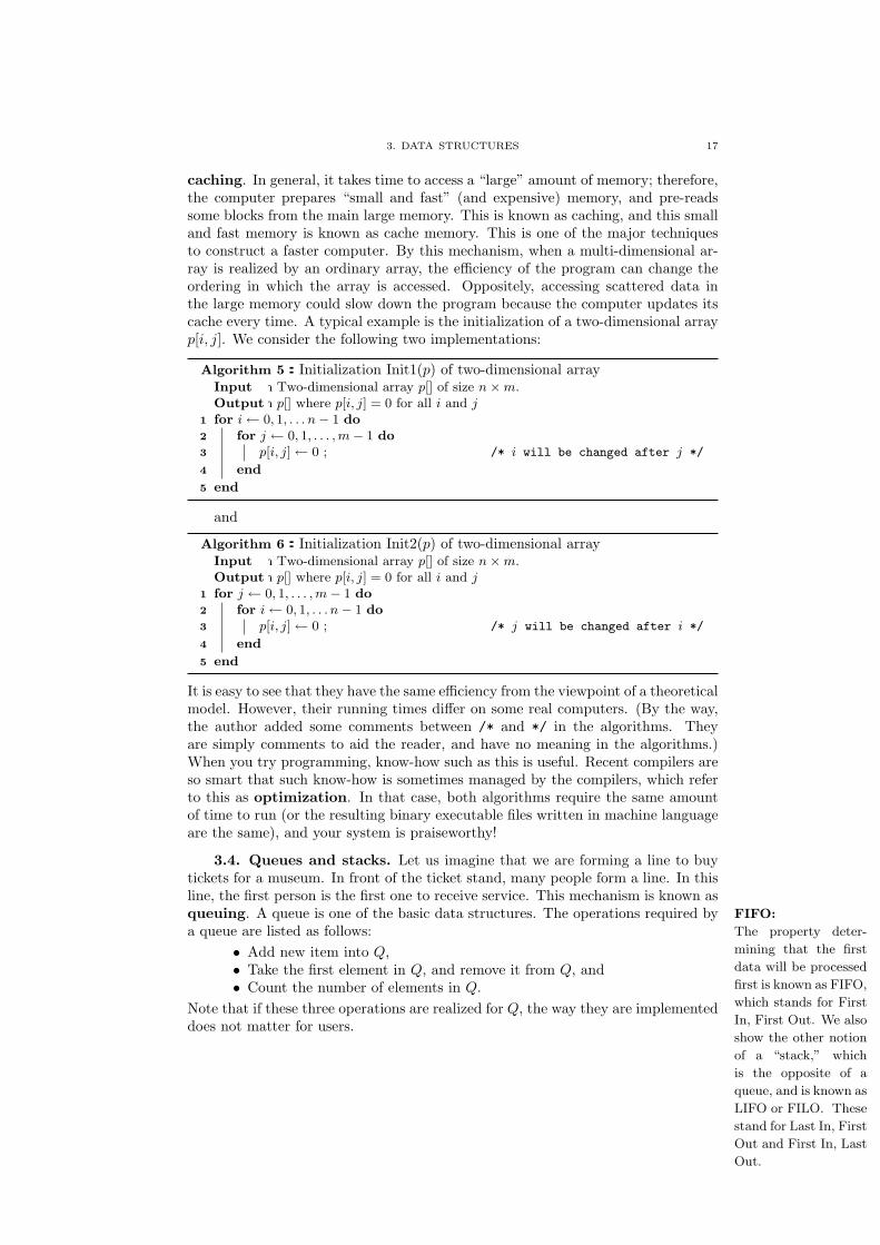
caching. In general, it takes time to access a “large” amount of memory; therefore,the computer prepares “small and fast” (and expensive) memory, and pre-readssome blocks from the main large memory. This is known as caching, and this smalland fast memory is known as cache memory. This is one of the major techniquesto construct a faster computer. By this mechanism, when a multi-dimensional ar-ray is realized by an ordinary array, the efficiency of the program can change theordering in which the array is accessed. Oppositely, accessing scattered data inthe large memory could slow down the program because the computer updates itscache every time. A typical example is the initialization of a two-dimensional arrayp[i, j]. We consider the following two implementations:

Algorithm 5：Initialization Init1(p) of two-dimensional arrayInput ：Two-dimensional array p[] of size n×m.Output ：p[] where p[i, j] = 0 for all i and j

1 for i← 0, 1, . . . n− 1 do2 for j ← 0, 1, . . . , m− 1 do3 p[i, j]← 0 ; /* i will be changed after j */

4 end

5 end

and

Algorithm 6：Initialization Init2(p) of two-dimensional arrayInput ：Two-dimensional array p[] of size n×m.Output ：p[] where p[i, j] = 0 for all i and j

1 for j ← 0, 1, . . . , m− 1 do2 for i← 0, 1, . . . n− 1 do3 p[i, j]← 0 ; /* j will be changed after i */

4 end

5 end

It is easy to see that they have the same efficiency from the viewpoint of a theoreticalmodel. However, their running times differ on some real computers. (By the way,the author added some comments between /* and */ in the algorithms. Theyare simply comments to aid the reader, and have no meaning in the algorithms.)When you try programming, know-how such as this is useful. Recent compilers areso smart that such know-how is sometimes managed by the compilers, which referto this as optimization. In that case, both algorithms require the same amountof time to run (or the resulting binary executable files written in machine languageare the same), and your system is praiseworthy!

3.4. Queues and stacks. Let us imagine that we are forming a line to buytickets for a museum. In front of the ticket stand, many people form a line. In thisline, the first person is the first one to receive service. This mechanism is known asqueuing. A queue is one of the basic data structures. The operations required by FIFO:

The property deter-

mining that the first

data will be processed

first is known as FIFO,

which stands for First

In, First Out. We also

show the other notion

of a “stack,” which

is the opposite of a

queue, and is known as

LIFO or FILO. These

stand for Last In, First

Out and First In, Last

Out.

a queue are listed as follows:• Add new item into Q,• Take the first element in Q, and remove it from Q, and• Count the number of elements in Q.

Note that if these three operations are realized for Q, the way they are implementeddoes not matter for users.

18 1. PRELIMINARIES

Next, let us again imagine that you accumulate unprocessed documents on yourdesk (the author of this book does not need to imagine this, because the situationis real). The documents are piled up on your desk. The bunch of paper crumble tothe touch; if you remove one from the middle of the pile, they will tumble down,and a great deal of damage will be done. Therefore, you definitely have to takeone from the top. Now we consider this situation from the viewpoint of sheets, inwhich case the service will be provided to the last (or latest) sheet first. That is,the process occurs in the order opposite to that in which they arrived. When datais processed by a computer, sometimes this opposite ordering (or LIFO) is moreuseful than queuing (or FIFO). Thus, this idea has also been adopted as a basicstructure. This structure is known as a stack. Similarly, the operations requiredby a stack S are as follows:

• Add new item into S,• Take the last element in S, and remove it from S, and• Count the number of elements in S.

The operations are the same as for a queue, with the only different point being theordering.

Both queues and stacks are frequently used as basic data structures. In fact,they are easy to implement by using an array with a few auxiliary variables. Herewe give the details of the implementation. First, we consider the implementation ofa queue Q. We use an array Q (Q[1], . . . , Q[n]) of size n and two variables s and t.The variable s indicates the starting point of the queue in Q, and the variable t isthe index such that the next item is stored at Q[t]. That is, Q[t] is empty, Q[t− 1]contains the last item. We initialize s and t as s = 1 and t = 1. Based on this idea,a naive implementation would be as follows.

Add a new element x into Q: For given x, substitute Q[t]← x, and up-date t← t + 1.

Take the first element in Q: Return Q[s], and update s← s + 1.Count the number of elements in Q: The number is given by t− s.

It is not difficult to see that these processes work well in general situations.However, this naive implementation contains some bugs (errors). That is, they donot work well in some special cases. Let us consider how we can fix them. Thereare three points to consider.

The first is that the algorithm tries to take an element from an empty Q. Inthis case, the system should output an error. To check this, when this operation isapplied, check the number of elements in Q beforehand, and output an error if Qcontains the zero element.

The next case to consider is that s > n or t > n. If these cases occur, moreprecisely, if s or t become n + 1, we can update the value by 1 instead of n + 1.Intuitively, by joining two endpoints, we regard the linear array Q as an array ofloop structure (Figure 5). However, we face another problem in this case: we cannotguarantee the relationship s ≤ t between the head and the tail of the queue anymore. That is, when some data are packed into Q[s], Q[s+1], . . . , Q[n], Q[1], . . . , Q[t]through the ends of the array, the ordinary relationship s < t turns around andwe have t < s. We can decide whether this occurs by checking the sign of t − s.Namely, if the number of elements of Q satisfies t − s < 0, it means the data arepacked through the ends of the array. In this case, the number of elements of Q isgiven by t− s + n.

3. DATA STRUCTURES 19

Q[1] Q[n]

Q[1] Q[n]

Q[n]Q[1]

Figure 5. Joining both endpoints of the array, we obtain a loopdata structure.

Exercise 6. When t − s < 0, show that the number of elements in thequeue is equal to t− s + n.

The last case to consider is that there are too many data for the queue. Theextreme case is that all Q[i]s contain data. In this case, “the next index” t indicates“the top index” s, or t = s. This situation is ambiguous, because we cannotdistinguish it from that in which Q is empty. We simplify this by deciding that thecapacity of this queue is n− 1. That is, we decide that t = s means the number ofelements in Q is zero, thereby preventing the nth data element from being packedinto Q. The last element of Q is useless, but we do not mind it for simplicity. Tobe sure, before adding a new item x into Q, the algorithm checks the number ofelements in Q. If x is the nth item, return “error” at this time, and do not add it.(This error is called overflow.)

Refining our queue with these case analyses enables us to safely use the queueas a basic data structure. Here we provide an example of the implementation ofour queue. The first subroutine is initialization:

Algorithm 7：Initialization of queue InitQ(n, t, s)Input ：The size n of queue and two variables t and sOutput ：An array Q as a queue

1 s← 1;

2 t← 1;

3 Allocate an array Q[1], . . . , Q[n] of size n;

Next we turn to the function “sizeof,” which returns the number of elementsin Q. By considering exercise 6, |t− s| < n always holds. Moreover, if t − s ≥ 0,it provides the number of elements. On the other hand, if t − s < 0, the queue isstored in Q[s], Q[s+1], . . . , Q[n], Q[1], . . . , Q[t]. In this case, the number of elementsis given by t− s + n. Therefore, we obtain the following implementation:

20 1. PRELIMINARIES

Algorithm 8：Function sizeof(Q) that returns the number of elements in Q.Input ：Queue QOutput ：The number of elements in Q

1 if t− s ≥ 0 then2 return t− s;

3 else4 return t− s + n;

5 end

When a new element x is added into Q, we have to determine whether Q isfull. This is implemented as follows:

Algorithm 9：Function push(Q, x) that adds the new element x into Q.Input ：Queue Q and element xOutput ：None

1 if sizeof(Q)= n− 1 then2 output “overflow” and halt;

3 else4 Q[t]← x;

5 t← t + 1;

6 if t = n + 1 then t← 1;

7 end

Similarly, when we take an element from Q, we have to check whether Q isempty beforehand. The implementation is shown below:

Algorithm 10：Function pop(Q) that takes the first element from Q andreturns it.

Input ：Queue QOutput ：The first element y in Q

1 if sizeof(Q)= 0 then2 output “Queue is empty” and halt;

3 else4 q ← Q[s];

5 s← s + 1;

6 if s = n + 1 then s← 1;

7 return q;

8 end

Note: In many programming languages, when a function F returns a value, thecontrol is also returned to the procedure that calls F . In pop(Q), it seems that wecan return the value Q[s] at line 4; however, then we cannot update s in lines 5 and6. Therefore, we temporally use a new variable q and return it in the last step.

It is easier to implement stack than queue. When using queue, we have tomanage the top element s and the tail element t; however, the top element of astack is fixed, thus we do not need to manage it by a variable. More precisely, wecan assume that S[1] is always the top element in the stack S. Therefore, the cyclicstructure in Figure 5 is no longer used. Based on this observation, it is not difficultto implement stack.

Exercise 7. Implement the stack S.

4. THE BIG-O NOTATION AND RELATED NOTATIONS 21

Some readers may consider these data structure to be almost the same as theoriginal one-dimensional array. However, this is not correct. These abstract modelsclarify the data properties. In Chapter 4, we will see a good example for using suchdata structure.

Next data structure of array? The next aspect of an array is called a “pointer.” If you understand arrays andpointers properly, you have learned the basics of a data structure. You canlearn any other data structure by yourself. If you have a good understandingof an array and do not know the pointer, the author strongly recommends tolearn it. Actually, a pointer corresponds to an address of the RAM machinemodel. In other words, a pointer points to some other data in a memory cell. Ifyou can imagine the notion of the RAM model, it is not difficult to understandthe notion of a pointer.

4. The big-O notation and related notations

As discussed in Section 2, the computational complexity of an algorithm A isdefined by using a function of the length n as input. Then we consider the worstcase analysis for many variants of inputs (there are 2n different inputs for length n).Even so, in general, the estimation of an algorithm is difficult. For example, even ifwe have an algorithm A whose time complexity fA(n) is fA(n) = 503n3 + 30n2 + 3if n is odd, and fA(n) = 501n3 + n + 1000 if n is even, what can we concludefrom them? When we estimate and compare the efficiency of algorithms, we haveto say that these detailed numbers have little meaning. Suppose we have anotheralgorithm B for the same problem that runs in fB(n) = 800n + 12345. In thissituation, for these two algorithms A and B, which is better? Most readers agreethat B is faster in some way. To discuss this intuition more precisely, D. E. Knuth(see page 49) proposed using the big-O notation. We will adopt this idea in thisbook. The key of the big-O notation is that we concentrate on the main factorof a function by ignoring nonessential details. By this notion, we can discuss andcompare the efficiency of algorithms independent from machine models. We focuson the asymptotic behavior of algorithms for sufficiently large n. This enables usto discuss the approximate behavior of an algorithm with confidence.

4.1. Warning. The author dares to give a warning before stating the defini-tion. The big-O notation is a notation intended as the upper bound of a function.That is, if an algorithm A solves a problem P in O(n2) time, intuitively, “the timecomplexity of algorithm A is bounded above by n2 within a constant factor for anyinput of length n.” We need to consider two points in regard to this claim.

• There may exist a faster algorithm than A. That is, to solve problem P ,while algorithm A solves it in O(n2) time, it may not capture the difficultyof P . Possibly, P can be solved much easier by some smart ideas.• This O(n2) provides an upper bound of the time complexity. We obtain

the upper bound O(n2) by analysis of the program that represents A insome way. However, the program may actually run in time proportionalto n. In this time, our analysis of the algorithm has not been appropriate.

22 1. PRELIMINARIES

The first point is not difficult to understand. There may be a gap betweenthe essential difficulty of the problem and our algorithm, because of the lack ofunderstanding of some properties of the problem. We provide such an examplein Section 2. Of course, there exist some “optimal” algorithms that cannot beimproved any further in a sense. In Section 3.5, we introduce such interestingalgorithms.

The second point is a situation that requires more consideration. For example,when you have f(n) = O(n2), even some textbooks may write this as “f(n) isproportional to n2.” However, this is wrong. Even if you have an algorithm Athat runs in O(n3), and another algorithm B that runs in O(n2), A can be fasterthan B when you implement and perform these algorithms. As we will see later,the notation “O(n3)” indicates that the running time of A can be bounded aboveby n3 in a constant factor. In other words, this is simply an upper bound of therunning time that we can prove. For the same reason, for one algorithm, withoutmodification of the algorithm itself, its running time can be “improved” from O(n3)to O(n2) by refining its analysis.

When you prefer to say “a function f(n) is proportional to n2” with accuracy,you should use the notation Θ(n2). In this book, to make the difference clear, wewill introduce O notation, Ω notation, and Θ notation. We also have o notationand ω notation, but we did not introduce them in this book. However, the Onotation is mainly used. That is, usually we need to know the upper bound of thecomputational resources in the worst case. For a novice reader, it is sufficient tolearn the O notation. However it is worth remembering that the O notation onlyprovides the upper bound of a function.

4.2. Big-O notation. We first give a formal definition of the O notation. Letg(n) be a function on natural numbers n. Then O(g(n)) is the set of functionsdefined as follows.

O notation:

O(g(n)) = f(n) | there exist some positive constants c and n0,for all n > n0, 0 ≤ f(n) ≤ cg(n) holds.

If a function f(n) on natural numbers n belongs to O(g(n)), we denote byf(n) = O(g(n)).

In this definition, we have some points to consider. First of all, O(g(n)) is aset of functions. Some readers familiar with mathematics may think “then, shouldit be denoted by f(n) ∈ O(g(n))?” This is correct. Some people denote it in thisway; however, they are (unfortunately) the minority. In this textbook, followingthe standard manner in this society, the author adopts the style f(n) = O(g(n)).That is, this “=” is not an equal to symbol in a strict sense. Although we write3n2 = O(n2), we never write O(n2) = 3n2. This “=” is not symmetrical! This isnot a good manner, which may throw beginners into confusion. However, in thistext book, we adopt the standard manner that is used in this society.

The next point is that we use n0 to avoid finite exceptions. Intuitively, thisn0 means that “we do not take care of finite exceptions up to n0.” For example,the function f1(n) in Figure 6 varies drastically when n is small, but stabilizeswhen n increases. In such a case, our interest focuses on the asymptotic behavior

4. THE BIG-O NOTATION AND RELATED NOTATIONS 23

n0

f1(n)

g(n)

f2(n)

f3(n)

Figure 6. Functions and the big O notation

for sufficiently large n. Therefore, using the constant n0, we ignore the narrowarea bounded by n0. If the behavior of f1(n) can be bounded above by g(n) forsufficiently large n, we denote it by f1(n) = O(g(n)).

We cannot ignore the constant c. By doing this, we can say that “we do nottake care of the constant factor.” For example, the function f2(n) is obtained fromg(n) by multiplying by a constant, and adding another constant. The philosophy ofthe big-O notation is that these “differences” are not essential for the behavior offunctions, and ignorable. This notion can be approximate, in fact, O(g(n)) containsquite a smaller function than g(n) such as f3(n) in Figure 6.

As learned in Section 1, an algorithm consists of a sequence of basic operations,and the set of basic operations depends on its machine model. Even in a realcomputer, this set differs depending on its CPU. That is, each CPU has its own setof basic operations designed by the product manufacturer. Therefore, when youimplement an algorithm, its running time depends on your machine. Typically,when you buy a new computer, you may be surprised that the new computer ismuch faster than the old one. To measure, compare, and discuss the efficiencyof algorithms in this situation, we require some framework that is approximate interms of “finite exceptions” and “constant factors.”

Exercise 8. For each of the following, prove it if it is correct, ordisprove it otherwise.

(1) 2n + 5 = O(n).(2) n = O(2n + 5).(3) n2 = O(n3).(4) n3 = O(n2).(5) O(n2) = O(n3).(6) 5n2 + 3 = O(2n).(7) f(n) = O(n2) implies f(n) = O(n3).(8) f(n) = O(n3) implies f(n) = O(n2).

24 1. PRELIMINARIES

How to pronounce “f(n) = O(n)” This “O” is simply pronounced “Oh”; thus, the equation can be pronouncedas “ef of en is equal to big-Oh of en.” However, some people also pronounce itas “ef of en is equal to order en.” 4.3. Other notations related to the big-O notation. We next turn to

the other related notations Ω and Θ, which are less frequently used than O. (Wealso have the other notations o and ω, which are omitted in this book. See thereferences for the details.)

In the broad sense, we call these O, Ω, Θ, o, and ω notations “the big-Onotations.” Namely, the most frequently used is the big-O notation. In this book,we will use “the big-O notation” that is used both in the broad sense and in thenarrow sense depending on the context.

Ω notation. Let g(n) be a function on natural numbers n. Then Ω(g(n)) is the setof functions defined as follows (it is pronounced as “big-omega” or simply “omega”).

Ω notation:

Ω(g(n)) = f(n) | there exist some positive integers c and n0,for all n > n0, 0 ≤ cg(n) ≤ f(n) holds.

If a function f(n) on natural numbers n belongs to Ω(g(n)), we denote byf(n) = Ω(g(n)).

Similar to the O notation, “=” is not a symmetric symbol.Comparing this with the O notation, the meaning of this Ω notation becomes

clearer. Two of their common properties are summarized as follows:

• We do not take care of finite exceptions under n0.• We do not mind a constant factor of c.

The difference is cg(n) ≤ f(n), that is, the target function f(n) is bounded frombelow by g(n).Trivial lower

bound:

To make sure, the

assumption that “all

data should be read

to solve a problem”

is quite a natural

assumption for most

problems. This lower

bound is sometimes

referred to as a trivial

lower bound.

That is, whereas the O notation is used to provide the upper bound of a func-tion, the Ω notation is used to provide the lower bound. Therefore, in the contextof computational complexity, the Ω notation is used to show a lower bound of someresources required to perform an algorithm. Here we give a trivial but importantexample. For some problem P with an input of length n, all input data should beread to solve the problem. Let an algorithm A solve the problem P in tA(n) time.Then we have tA(n) = Ω(n). That is, essentially, tA(n) cannot be less than n.

In Chapter 3, we will see a more meaningful example of the Ω notation.

Θ notation. Let g(n) be a function on natural numbers n. Then Θ(g(n)) is theset of functions defined as follows (it is pronounced as “theta”).

Θ notation:

5. POLYNOMIAL, EXPONENTIAL, AND LOGARITHMIC FUNCTIONS 25

Θ(g(n)) = f(n) | there exist some positive constants c1, c2, and n0,for all n > n0, 0 ≤ c1g(n) ≤ f(n) ≤ c2g(n) holds.

If a function f(n) on natural numbers n belongs to Θ(g(n)), we denote it byf(n) = Θ(g(n)).

Considering O(g(n)), Ω(g(n)), and Θ(g(n)) as sets of functions, we can observethe following relationship among them:

Θ(g(n)) = O(g(n)) ∩ Ω(g(n))

That is, Θ(g(n)) is an intersection of O(g(n)) and Ω(g(n)).

Exercise 9. Prove the above equation Θ(g(n)) = O(g(n)) ∩ Ω(g(n)).

Checking the O and Ω notations, let us consider the meaning of the equationf(n) = Θ(g(n)). The following two margins are again available:

• We do not take care of finite exceptions under n0.• We do not mind a constant factor of c.

Within these margins, f(n) is bounded by g(n) both above and below. That is, wecan consider f(n) to be proportional to g(n). In other words, f(n) is essentiallythe same function as g(n) within a constant factor with finite exceptions.

There are some algorithms of which the behavior has been completely analyzed,and their running times are already known. For these algorithms, their efficiencycan be represented in Θ notation with their accuracy independent of machine mod-els. Some examples are provided in Chapter 3.

5. Polynomial, exponential, and logarithmic functions

Let A be an algorithm for some problem, and assume that its running timefA(n) is fA(n) = 501n3 +n+1000 for any input of length n. When we measure theefficiency of an algorithm, discussion about the detailed coefficients is not produc-tive in general. Even if we “improve” the algorithm and obtain a new complicatedalgorithm A′ that runs in fA′(n) = 300n3 + 5n, it may be better to update thecomputer and perform A on it. The real running time of A may vary depending onthe programmer’s skill and the machine model.

Therefore, we usually estimate the running time of an algorithm A by using theO notation introduced in Section 4 as fA(n) = O(n3). Once you become familiarwith algorithm design, it may not be rare that you discover some redundant process,refine it, and obtain an algorithm that is, say, n times faster. Therefore, from thisviewpoint, even if you improve your algorithm from 501n3 to 300n3, it is unlikelythat this essentially improves the algorithm.

When we evaluate the computational complexity of some problems, we fre-quently take a global view of the difficulty. If you like to solve some specific prob-lem, in most cases, the problem has some solution, and moreover, even choicesare also given. In this case, how about the idea of “checking all possibilities”?That is, from the initial state, checking all possible choices, we eventually reachthe solution, don’t we? In most cases, this naive intuition is theoretically correct.However, theoretically it is true. For example, consider a well-known popular gamesuch as Shogi. The board is fixed. Its size is 9 × 9, that is, we have at most 81choices at each step. The number and kinds of pieces are also fixed. The rules of

26 1. PRELIMINARIES

the game are also strictly designed. Then, theoretically, if both players play withtheir best possible strategies, the game is decided by one of three outcomes: thefirst player always wins, the second player always wins, or the game is tie. Thatis, the end of the game has already been decided, even though we do not yet knowwhich is the true end. We would be able to reach the true outcome by checking allpossible choices. A program for checking all choices would not seem difficult to askillful programmer. However, so far, nobody knows the true outcome for a gameof chess, Shogi, Go, and so on. This is because such a program never completes itscomputation. Even in the case of the board consisting of only 9 × 9 squares, thenumber of choices runs into astronomical numbers, and the computation cannot becompleted in a realistic time.

Here we again consider the fact that the Shogi board only has a size of 81.When we consider current computers, which have gigabytes of memory and run atgigahertz, the number 81 seems to be quite small compared to these specifications.Nevertheless, why does the algorithm never complete its computation? The key isa phenomenon known as “exponential explosion.” To understand this phenomenonwith related ideas, we can partition the functions in this book into three categories:polynomial functions, exponential functions, and logarithmic functions. When weconsider the efficiency of an algorithm (from the viewpoints of both time and mem-ory), at the first step, it is quite important to have a clear view as to the categoryof the running time and memory used. We will describe these three categories offunctions with some intuitive image.

Polynomial function. For example, a quadratic function is a typical polynomialfunction. It is the most natural “function” people imagine when they say function.In general, a polynomial function is defined as follows.

Polynomial function:A polynomial function is given in the following form:

f(x) = adxd + ad−1x

d−1 + · · ·+ a3x3 + a2x

2 + a1x + a0,

where a0, a1, . . . , ad are constant numbers independent of x, and d is a naturalnumber. More precisely, d is the maximum number with ad 6= 0, and d isreferred to as the degree of this function f(x).

In terms of computational complexity, if any computational resource is notincluded in this class, it is said to be intractable. That is, even if the problem hasa simple solution (e.g., 0/1 or Yes/No), and we can build a program for it (e.g., byexhaustive check of all combinations), the intractable problem cannot be solved inpractical time. Here we note that this sentence contains a double negative; thatis, any problem not included in this class cannot be solved in practical time. Wenever say that all problems in this class are tractable. This does not aim to confusereaders. There is a gray zone between tractable and intractable. For example,suppose you succeed in developing an algorithm A that requires fA(n) = Θ(nd) torun. Even if fA(n) is a polynomial function, it can be quite difficult to obtain asolution in practical time when d is quite large, for example 1000 or 20000. From apractical viewpoint, a reasonable value of d is not so large, say, d = 2, 3 or up to 10.Of course, this “reasonable” is strongly related to the value of n, the specification ofthe computer, the skill of programmer, and so on. However, at least, fA(n) cannotbe bounded above by some polynomial function, fA(n) increases drastically whenn becomes large, and the program never halts in a practical time.

5. POLYNOMIAL, EXPONENTIAL, AND LOGARITHMIC FUNCTIONS 27

Exercise 10. Let the running time fA(n) of an algorithm A be n50

steps. That is, the algorithm A performs n50 basic operations for any input of sizen to compute the answer. Suppose that the processor of your computer executesinstructions at a clock speed of 10GHz. That is, your computer can perform 10 ×109 basic operations per second. Compute the value of n such that your computerperforms the algorithm A for an input of size n in a practical time.

Exercise 11. Let us consider algorithms for computing the following poly-nomial function:

f(x) = a0 + a1x + a2x2 + + · · ·+ ad−1x

d−1 + adxd

Suppose that an array a[] stores each coefficient with a[i] = ai, and we want tocompute f(x) for any given x. We first consider a naive algorithm that computesin the way of a0 + a1 × x + a2 × x× x + · · ·+ ad−1 × x× · · · × x + ad × x× · · · × xstraightforwardly. Then, how many additions and multiplications does the naivealgorithm perform? Next, we transform the equation and use the second algorithmto perform the following computation:

f(x) = a0 + x× (a1 + x× (a2 + x× (a3 + · · ·+ x× (ad−1 + x× ad) · · · ))).Then, how many additions and multiplications does the second algorithm perform?

Exponential function. Typically, an exponential function is the xth power of aconstant such as 2x. We introduce a more general form as follows:

Exponential function:An exponential function is f(x) = cx for some constant c with c > 1.

When we consider the resources of algorithms, as we only consider increasingfunctions, we may have c > 1 in general. When c > 1, any exponential functiongrows quite rapidly, which is counter-intuitive. This phenomenon is known asexponential explosion. For example, consider a board game such as Shogi, whichallows us some choices. If we have two choices in every turn, if you try to readpossible situations after ten turns, you will have to check 210 = 2×2×· · ·×2 = 1024possible cases. (Of course, different choices can imply the same situation, and wehave more choices in general; hence, we have to give more careful considerationto the real situation.) It may seem that this number of cases is an easy task forcurrent computers. Anyway, try the following exercise.

Exercise 12. Take a sheet of newspaper. First, fold it in half. Next,fold it in half again. Repeat the folding until you cannot fold it any more. Howmany times can you fold it? Can you fold it beyond ten times? Let the thickness ofthe newspaper be 0.1mm. How many times do you have to fold it in half until thethickness (or height) of the sheet exceeds that of Mt. Fuji (3776m)? Moreover, howmany times do you have to fold it to go beyond the distance between the moon andEarth (around 38× 104km)?

After solving this exercise, you will find that you can go to the moon justby folding a sheet of paper relatively “few times”. This “strange incompatibility”with your intuition is the reason why it is difficult to realize the tremendousness ofexponential functions.

When we design an algorithm for some problem, it is not difficult to developan exponential time algorithm in general. The naive idea of “checking all possible

28 1. PRELIMINARIES

cases” tends to lead us to an algorithm requiring exponential time. It is a veryimportant key point to develop a polynomial time algorithm in some way. Thatrequires us to understand the problem deeply, and, by identifying the nontrivialproperties of the problem one by one enables us to reach more efficient, faster, andelegant algorithms.

Logarithmic function. We have already seen that exponential functions grow ex-pansively. When you plot an exponential function y = f(x) on the usual Cartesiancoordinate system, the curve rises rapidly, immediately rising beyond any graphpaper. A logarithmic function is obtained by folding or reflecting some exponentialcurve along the 45 line y = x.

Logarithmic function:For an exponential function f(x) = cx, its inverse function g(x) = logc x is alogarithmic function. We sometimes omit the base and write it as log x whenthe base c is 2. When the base c is e = 2.718 · · · , the natural logarithmicfunction loge x is denoted by lnx.

Because a logarithmic function is an inverse function of some exponential func-tion, the logarithmic function y = f(x) grows very slowly even if x becomes quitelarge.

For example, when you use 8 bits, you can distinguish 28 = 256 cases, and 16bits lead us to 216 = 65536 cases. An increase of 1 bit causes the number of dis-tinguishable cases to double. This rapid increase is the property of an exponentialfunction. For logarithmic functions, the situation is inverse; even if 65536 caseswere to rapidly increase up to twice as much, i.e., 131072, it is sufficient to addonly 1 bit to the 16-bit information. That is, for the same reason that an exponen-tial function grows with counterintuitive speed, a logarithmic function grows withcounterintuitive slowness.

Exercise 13. Draw three graphs of f(x) = 2x, f(x) = x, and f(x) =log x for 1 ≤ x ≤ 20.

l’Hospital’s rule In this book, we conclude that any exponential function f(n) = cn with c > 1grows much faster than any polynomial function g(n) for sufficiently large nwith intuitive explanation. Precisely, we do not give any formal proof of thefact g(n) = O(f(n)). For example, we can say that n100 = O(1.01n). However,unfortunately, its formal and mathematical proof is not so easy. A simple proofcan be performed by using l’Hospital’s rule that is a theorem about differen-tial functions. By l’Hospital’s rule, for two functions f(n) and g(n) (with someomitted conditions here), we have limn→∞ f(n)/g(n) = limn→∞ f ′(n)/g′(n).In our context, we can differentiate any number of times. We can observe thatany polynomial function g(n) = O(nd) for some positive integer d becomes aconstant after differentiating d times. On the other hand, any exponential func-tion f(n) will still be exponential function after d differentiations. (Typically,differentiating f(n) = en becomes f ′(n) = en again.) Therefore, for example,after 100 differentiations of n100/1.01n, we have limn→∞ n100/1.01n = 0, whichimplies n100 = O(1.01n).

5. POLYNOMIAL, EXPONENTIAL, AND LOGARITHMIC FUNCTIONS 29

Desk

Card 1

Gravity center of card 1

Edge of card 2

Card 2

Length 1

Figure 7. Card stack problem

5.1. Harmonic number. Analyses of algorithms sometimes leads us to im-pressive equations. In this section, we demonstrate one of them known as harmonicnumber. The definition of the nth harmonic number H(n) is as follows. Harmonic number:

In the wide sense, the

harmonic number is

defined by the sum-

mation of the inverse

of the sequence of

numbers with a com-

mon difference (or the

denominators are a

sequence of numbers

with a common differ-

ence), in the narrow

sense, the simplest se-

quenceP∞

i=11i

is used

to define the harmonic

number.

The nth harmonic number H(n):

H(n) =n∑

i=1

1i

=11

+12

+ · · ·+ 1n

That is, the summation of the first n elements in the harmonic series∑∞

i=11i

is known as the nth harmonic number, which is denoted by H(n). The harmonicnumber has quite a natural form, and it has the following interesting property.

limn→∞

(H(n)− lnn) = γ,

where γ is an irrational number γ = 0.57721 . . . known as Euler’s constant. Thatis, H(n) is very close to ln n, with quite a small error.

We do not pursue this interesting issue in any detail; rather, we simply usethe useful fact that the nth harmonic number is almost equal to ln n. Theharmonic number is in natural form, and hence it sometimes appears in the analysisof an algorithm. We will encounter it a few times. Intuitively, the harmonic numbergrows quite slowly as n increases, because it is almost ln n.

Card stack problem. Here we will see a typical situation in which the harmonicnumber appears. You have quite a number of cards. You would like to stack thecards on your desk such that the card at the top protrudes beyond the edge of thedesk. Then, how far can you position the card? Intuitively, it seems impossibleto position the topmost card such that the entire card protrudes beyond the desk.Are you sure about this?

In reality, you have to stack the cards from bottom to top, of course. However,to simplify the explanation, we reverse the time and first consider the last card. (We

30 1. PRELIMINARIES

Card 1

Gravity center of card 1

Card 2

Length 1

Length x2

Gravity center of (card 1 + card 2)

Length 1

Gravity center of card 2

Figure 8. The center of gravity of the top two cards 1 and 2

might consider slipping in a card at the bottom of the stack at each step.) Withoutloss of generality, our card has the width 2 and weight 1. Cards are identified bynumbering them as 1, 2, 3, . . . from the top.

Let us consider the card at the top, card 1. We position this card as far asthe edge of the next card, card 2 (Figure 7). At the limit, the center of card 1is on the edge of card 2. That is, card 1 can be moved beyond half of its length(or length 1) from card 2. The next step is for positioning card 2. Let x2 be thelength between the center of gravity of these two cards and the right edge of card2 (Figure 8). Then, at this point the centers of cards 1 and 2 are balanced in asee-saw manner (distance × weight), that is, they are balanced at the right and leftsides. Therefore, (1− x2)× 1 for the left card 2, and x2× 1 for the right card 1 arebalanced. That is, we have

(1− x2)× 1 = x2 × 1,

and hence x2 = 1/2.We have to put our heart into the next step for card 3. The center of gravity

of the two cards 1 and 2 lies at 1/2 from the right side of card 2. We consider thefulcrum that maintains a balance between the right edge of card 3, on top of whichcards 1 and 2 are placed, and the center of card 3. Let x3 be the distance of thisbalance point from the right side of card 3. Then, similarly, we have

(1− x3)× 1 = x3 × 2.

Note that we have ×2 on the right hand because we have two cards on the rightside. Solving this, we obtain x3 = 1/3.

We can repeat this process; for the card k, we have k − 1 cards on it. Weconsider that the gravity center of these k − 1 cards occurs on the right edge ofcard k, and we balance it with the center of card k at the point distance xk fromthe right side of card k. Then we have

(1− xk)× 1 = xk × (k − 1),

and obtain xk = 1/k.

5. POLYNOMIAL, EXPONENTIAL, AND LOGARITHMIC FUNCTIONS 31

Summarizing, when we stack n cards in this way, the distance of the right edgeof card 1 from the edge of the desk is given by the following equation.

1 +12

+13

+ · · ·+ 1n

=n∑

i=1

1i

We can observe that 1+1/2+1/3 = 11/6 < 2 < 1+1/2+1/3+1/4 = 25/12, whichmeans that if we stack only four cards neatly, the first card protrudes beyond theedge of the desk. That is, beneath card 1, we have nothing but cards. Actually, itis not that easy; however, it is worth trying just for fun (Figure 3 in page 134).

Now we consider the last function∑n

i=11i . This is exactly the harmonic number

H(n). As we have already seen, the harmonic number H(n) is almost equal to lnn.Moreover, the function lnn is a monotonically increasing function for n. Therefore,when you pile up many cards, you can position card 1 as far from the edge of thedesk as you prefer. We must agree that this is counterintuitive. Then, how manycards do we have to pile up to make the card protrude farther?

Exercise 14. We have already observed that we need four cards to obtainthe distance 2, which is the width of one card. Then how many cards do we needto increase this distance to 4, which is the width of two cards. How many cards dowe have to prepare to increase this distance to 10 for five cards?

Solving Exercise 14, we realize that it is not as easy to achieve a large distance.That is, to increase a logarithmic function f(n) to become large, we have to sub-stitute a very large value into n. This is essentially the same as the exponentialexplosion. As an exponential function g(n) increases quite rapidly as n increases,to increase the size of a logarithmic function f(n), we have to increase the value ofn considerably.

Have curiousness! Theoretically, we can position the first card as far as you prefer by using thestacking method described in the text. However, if you prefer to obtain a largedistance, we need a very large number of cards, as we have already seen. Infact, the above discussion with the result H(n) is itself a well-known classicresult in the society of recreational mathematics and puzzles. Then, can wereduce the number of cards to obtain some distance? In other words, is theabove method the optimal way to ensure the card at the top protrudes farther?When you consider the method locally, as you put every card on the edge ofbalance in each step, at a glance it seems impossible to improve.However, surprisingly, recently (in 2006) it was shown that this method is notoptimal, and we can reduce the number of cards in general!a That is, wehave algorithms that are more efficient for stacking cards. Honestly, as theauthor himself never imagined that this method might be improved, he wasvery surprised when he heard the presentation about the improved algorithm.Aside from the details of the algorithm, the author had to take his hat off totheir idea that the classic method might not be optimal.

aMike Paterson and Uri Zwick, “Overhang,” Proceedings of the 17th annual ACM-SIAMsymposium on Discrete algorithm, pp. 231–240, ACM, 2006.

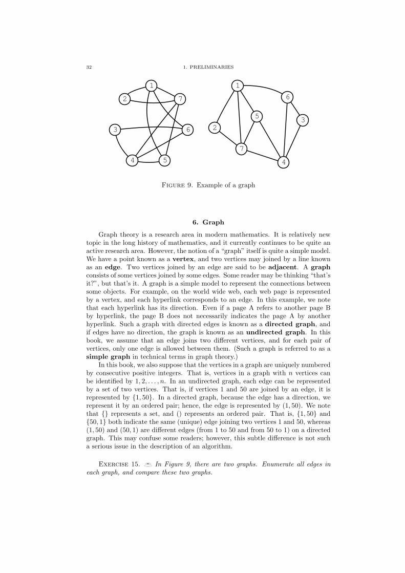
32 1. PRELIMINARIES

2

1

5

7

4

6

3

2

1

5

7

4

63

Figure 9. Example of a graph

6. Graph

Graph theory is a research area in modern mathematics. It is relatively newtopic in the long history of mathematics, and it currently continues to be quite anactive research area. However, the notion of a “graph” itself is quite a simple model.We have a point known as a vertex, and two vertices may joined by a line knownas an edge. Two vertices joined by an edge are said to be adjacent. A graphconsists of some vertices joined by some edges. Some reader may be thinking “that’sit?”, but that’s it. A graph is a simple model to represent the connections betweensome objects. For example, on the world wide web, each web page is representedby a vertex, and each hyperlink corresponds to an edge. In this example, we notethat each hyperlink has its direction. Even if a page A refers to another page Bby hyperlink, the page B does not necessarily indicates the page A by anotherhyperlink. Such a graph with directed edges is known as a directed graph, andif edges have no direction, the graph is known as an undirected graph. In thisbook, we assume that an edge joins two different vertices, and for each pair ofvertices, only one edge is allowed between them. (Such a graph is referred to as asimple graph in technical terms in graph theory.)

In this book, we also suppose that the vertices in a graph are uniquely numberedby consecutive positive integers. That is, vertices in a graph with n vertices canbe identified by 1, 2, . . . , n. In an undirected graph, each edge can be representedby a set of two vertices. That is, if vertices 1 and 50 are joined by an edge, it isrepresented by 1, 50. In a directed graph, because the edge has a direction, werepresent it by an ordered pair; hence, the edge is represented by (1, 50). We notethat represents a set, and () represents an ordered pair. That is, 1, 50 and50, 1 both indicate the same (unique) edge joining two vertices 1 and 50, whereas(1, 50) and (50, 1) are different edges (from 1 to 50 and from 50 to 1) on a directedgraph. This may confuse some readers; however, this subtle difference is not sucha serious issue in the description of an algorithm.

Exercise 15. In Figure 9, there are two graphs. Enumerate all edges ineach graph, and compare these two graphs.

6. GRAPH 33

2 1

5

7

4

6

3

2

1

5

7

4

63

Figure 10. An example of a tree

A graph is a very simple but strong model and has many interesting properties.Here we introduce three theorems that show useful properties for the analysis ofalgorithms, with two proofs for them.

The first theorem is about the degrees of an undirected graph. The degreed(i) of a vertex i in an undirected graph is the number of vertices that are adjacentto vertex i. In other words, d(i) is the number of edges joined to the vertex i. Forthe degrees of a graph, the following theorem is well known.

Theorem 3. In an undirected graph, the summation of the degrees of the ver-tices is equal to twice the number of edges.

Exercise 16. Compare the summation of the degrees of the vertices in thegraph in Figure 9 with the number of edges.

Theorem 3 seems to be strange, but can be proved elegantly by changing theviewpoint.

Proof. Observe the operation “add d(i) for each vertex i” from the viewpointof an edge. Each edge i, j is counted from vertex i and vertex j. That is, each edgeis counted twice. Therefore, in total, the summation becomes twice the number ofedges.

Exercise 17. For a vertex i in a directed graph, the number of edgesfrom the vertex i is referred to as out-degree, and the number of edges to thevertex i is referred to as in-degree. Then, develop an analogy of Theorem 3 fordirected graphs.

Next, we introduce a special class of graphs known as trees. On an undirectedgraph, if any pair of vertices is joined by some sequence of edges, this graph isconsidered to be connected. For a connected graph, if any pair of vertices hasa unique route between them, this graph termed a tree. Intuitively, a tree hasno cycle; otherwise, we would have some pair of vertices with two or more routesbetween them. Formally, a graph is a tree if and only if it is connected and acyclic.We here show two examples of trees in Figure 10. There is an interesting theoremfor trees.

Theorem 4. Any tree with n vertices has exactly n− 1 edges. Oppositely, anyconnected graph with n− 1 edges is a tree.

34 1. PRELIMINARIES

There are exponentially many trees with n vertices. Nevertheless, every treehas the same number of edges if the number of vertices is fixed. It is an impressivefact. In fact, two trees in Figure 10 have seven vertices with six edges. From theviewpoint of algorithm design, as we will see, the intuition that “any tree with nvertices has almost n edges” is useful. The proof of Theorem 4 is not simple andwe omit from this book. However, this theorem is one of the basic and importanttheorems in graph theory, and it is easy to find the proof in standard textbooks ongraph theory.

Each vertex of degree 1 in a tree is known as a leaf. The following theorem issimple and useful.

Theorem 5. Every tree with at least two vertices has a leaf.

Proof. It is trivial that a tree with two vertices consists of two leaves. Weconsider any tree T that has three or more vertices. Suppose that this T has noleaves. Because T is connected, every vertex has a degree of at least 2. Therefore, byTheorem 3, for m number of edges, we have 2m =

∑each vertex v d(v) ≥ 2×n = 2n,

which implies m ≥ n. However, this contradicts the claim m = n − 1 in Theorem4. Therefore, any tree has a vertex of degree one.

Examining the two trees in Figure 10, the left tree has two leaves (vertices 1and 7), and the right tree has four leaves (vertices 2, 3, 4, and 7). In fact, Theorem5 can be strengthened to “every tree with at least two vertices has at least twoleaves.” However, in this book, we only need the fact that every nontrivial tree hasa leaf.

Theorem 5 is useful when we design an algorithm that functions on a treestructure. Suppose we would like to solve some problem P defined on a tree T .Then, by Theorem 5, T has to have a leaf. Thus, we first solve P on the leafvertex. Then, we remove the useless (or processed) vertex with its associated edge.This leaf is of degree one; hence, the tree is still connected after removing the leaf.Moreover, the condition in Theorem 4 still holds because we have removed onevertex and one edge. That is, after removing the leaf the graph continues to be atree, and we again have another unprocessed leaf. In this way, we can repeatedlyapply the same algorithm to each leaf, reducing the graph one by one, and finally,we have a trivial graph with one vertex. Even problems that are difficult to solveon a general graph, can sometimes be solved efficiently on a tree in this way.

6.1. Representations of a graph. When we process a graph by computer,we have to represent the graph in memory in some ways. There are two typicalapproaches for representing a general graph. Mainly, the first approach is usedwhen the algorithm is concerned with the neighbors of each specified vertex, andthe second approach is used when the algorithm processes the whole graph structureat once. Both ways have their advantages; thus, we choose one of them (or the otherspecified way) according to the main operations in the algorithm.

Representation by adjacency set. The vertices adjacent to a vertex i arerepresented by an adjacency set. That is, the neighbor set N(i) for a vertex i in anundirected graph is defined by

N(i) = j | there is an edge i, j in the graph,

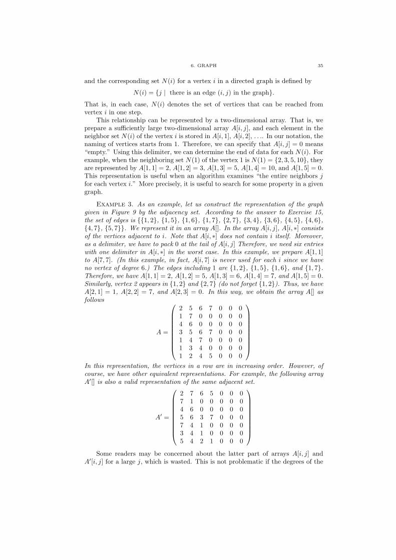
6. GRAPH 35

and the corresponding set N(i) for a vertex i in a directed graph is defined by

N(i) = j | there is an edge (i, j) in the graph.

That is, in each case, N(i) denotes the set of vertices that can be reached fromvertex i in one step.

This relationship can be represented by a two-dimensional array. That is, weprepare a sufficiently large two-dimensional array A[i, j], and each element in theneighbor set N(i) of the vertex i is stored in A[i, 1], A[i, 2], . . .. In our notation, thenaming of vertices starts from 1. Therefore, we can specify that A[i, j] = 0 means“empty.” Using this delimiter, we can determine the end of data for each N(i). Forexample, when the neighboring set N(1) of the vertex 1 is N(1) = 2, 3, 5, 10, theyare represented by A[1, 1] = 2, A[1, 2] = 3, A[1, 3] = 5, A[1, 4] = 10, and A[1, 5] = 0.This representation is useful when an algorithm examines “the entire neighbors jfor each vertex i.” More precisely, it is useful to search for some property in a givengraph.

Example 3. As an example, let us construct the representation of the graphgiven in Figure 9 by the adjacency set. According to the answer to Exercise 15,the set of edges is 1, 2, 1, 5, 1, 6, 1, 7, 2, 7, 3, 4, 3, 6, 4, 5, 4, 6,4, 7, 5, 7. We represent it in an array A[]. In the array A[i, j], A[i, ∗] consistsof the vertices adjacent to i. Note that A[i, ∗] does not contain i itself. Moreover,as a delimiter, we have to pack 0 at the tail of A[i, j] Therefore, we need six entrieswith one delimiter in A[i, ∗] in the worst case. In this example, we prepare A[1, 1]to A[7, 7]. (In this example, in fact, A[i, 7] is never used for each i since we haveno vertex of degree 6.) The edges including 1 are 1, 2, 1, 5, 1, 6, and 1, 7.Therefore, we have A[1, 1] = 2, A[1, 2] = 5, A[1, 3] = 6, A[1, 4] = 7, and A[1, 5] = 0.Similarly, vertex 2 appears in 1, 2 and 2, 7 (do not forget 1, 2). Thus, we haveA[2, 1] = 1, A[2, 2] = 7, and A[2, 3] = 0. In this way, we obtain the array A[] asfollows

A =

2 5 6 7 0 0 01 7 0 0 0 0 04 6 0 0 0 0 03 5 6 7 0 0 01 4 7 0 0 0 01 3 4 0 0 0 01 2 4 5 0 0 0

In this representation, the vertices in a row are in increasing order. However, ofcourse, we have other equivalent representations. For example, the following arrayA′[] is also a valid representation of the same adjacent set.

A′ =

2 7 6 5 0 0 07 1 0 0 0 0 04 6 0 0 0 0 05 6 3 7 0 0 07 4 1 0 0 0 03 4 1 0 0 0 05 4 2 1 0 0 0

Some readers may be concerned about the latter part of arrays A[i, j] and

A′[i, j] for a large j, which is wasted. This is not problematic if the degrees of the

36 1. PRELIMINARIES

vertices are almost equal; instead, there would be reason for concern if they wereextremely varied such as the graph representing Web pages (see page 36). In sucha case, the use of pointers (which is beyond the scope of this book) instead of anarray, would enable us to construct a more efficient data structure.

Representation by adjacency array. In an adjacency array representation, weagain use a two-dimensional array A[i, j]; however, element [i, j] directly indicatesedge (i, j) or i, j. That is, if A[i, j] = 0 we have no edge between two verticesi and j, and A[i, j] = 1 means there is an edge joining the vertices i and j. Thisrepresentation is not efficient for a large graph with a few edges from the viewpointof memory usage. On the other hand, some algorithms run fast because they areable to determine whether the graph contains the edge i, j in one step. Moreover,this representation is extensible to graphs with weighted edges; in this case, A[i, j]provides the weight of the edge i, j. When we consider an undirected graph, wehave A[i, j] = A[j, i]. Usually, the diagonal elements A[i, i] are set to be 0.

Example 4. Here we again consider the graph in Figure 9 and represent itby an adjacency array. This time, we write 1 if the graph has the correspondingedge, and 0 if not. For example, for the edge 1, 2, we write 1s for both of the(1, 2) element and the (2, 1) element in the array. However, for the pair 3, 5, wehave no edge between vertices 3 and 5; hence, we write 0s at both for the (3, 5) and(5, 3) elements. We also define (i, i) as 0 for every i, then the resulting adjacencyarray A′′[] for the edge set 1, 2, 1, 5, 1, 6, 1, 7, 2, 7, 3, 4, 3, 6, 4, 5,4, 6, 4, 7, 5, 7 is represented as follows:

A′′ =

0 1 0 0 1 1 11 0 0 0 0 0 10 0 0 1 0 1 00 0 1 0 1 1 11 0 0 1 0 0 11 0 1 1 0 0 01 1 0 1 1 0 0

Note that we have a unique A′′ unlike an adjacency set because the indices of thevertices are fixed. In an undirected graph, we always have A′′[i, j] = A′′[j, i], thatis, A′′ is a symmetric matrix. In this representation, each entry is either 0 or 1.

Link structure of WWW It is known that the graph representing the link structure of the WWW (WorldWide Web) has a property referred to as scale free. In a scale free graph, mostvertices have quite small sets of neighbors, whereas few vertices have quite largesets of neighbors. Considering real WWW pages, many WWW pages containa few links that are maintained by individual people; however, as for a searchengine, few WWW pages contain a large number of links. In this book, weintroduce two different representations for graphs. Unfortunately, none of themwould be able to efficiently (from the viewpoint of memory usage) maintain ahuge scale-free graph. This would require a more sophisticated data structure.

CHAPTER 2

Recursive call

bababababababababababababababab

Recursive call may appear difficult when you initially approach, but it can-not be overlooked when it comes to studying algorithms. It bears a closeconnection with mathematical induction, and those who once had a frus-trating experience with mathematical induction in the past may feel intim-idated, but there is nothing to fear. It is the author’s opinion that anyonewho understands grammatically correct your native language and knowshow to count natural numbers can master the use of recursive calls. Inthis chapter, we will attempt to understand recursive calls and their cor-rect usage by considering two themes: the “Hanoi tower” and “Fibonaccinumbers.”

What you will learn: • Recursive call• Hanoi tower• Fibonacci numbers• Divide-and-conquer• Dynamic programming

37

38 2. RECURSIVE CALL

Figure 1. Tower of Hanoi with 7 discs

1. Tower of Hanoi

Under a dome that marks the center of the world in a great temple in Benares,India, there are three rods. In the beginning of the world, God piled 64 discs ofpure gold onto one of the rods in descending order of size from bottom to top.Monks spend days and nights transferring discs from rod number 1 to rod number3 following a certain rule. The world is supposed to end as soon as the monks finishmoving all the discs. The rules for moving the discs around are quite simple. In thefirst place, only one disc can be moved at a time. Moreover, a disc cannot be placedupon a smaller one. How can the monks move the disks in an efficient manner?Moreover, how many times would the monks have to move the discs around tofinish moving all discs?

This puzzle is known as the Tower of Hanoi. It was originally proposed in 1883by French mathematician E. Lucas. An example of the Tower of Hanoi availablein the market is shown in Figure 1. This example has seven discs. In this chapter,we will consider algorithms to move discs and the number of moves H(n), where nis the number of discs.

We simplify descriptions by denoting the transfer of disc i from rod j to rodk as (i; j → k). Consider that the discs are enumerated in ascending order ofsize, starting from the smallest one. Let us start with a simple case, which is aconvenient way to familiarize ourselves with the operation. The simplest case isof course for n = 1. If there is only one disc, it is straightforward to performoperation (1; 1→ 3), which consists of simply moving the disc from rod 1 to rod 3;thus, H(1) = 1. Next, let us consider the case n = 2. In the beginning, the onlyoperations that are possible are (1; 1 → 3) or (1; 1 → 2). As we eventually want

1. TOWER OF HANOI 39

Figure 2. View of the transitions of the Tower of Hanoi for n = 3

to execute (2; 1 → 3), we choose the latter alternative. With a little thought, it isnot difficult to conclude that the best operations are (1; 1 → 2), (2; 1 → 3), and(1; 2→ 3). Therefore, H(2) = 3. At this point, we start getting confused for valuesof n = 3 or greater. After some thought, we notice the following three points:

• We necessarily have to perform operation (3; 1→ 3).• Operation (3; 1 → 3) requires all discs except 3 to be moved from rod 1

to rod 2.• After performing (3; 1 → 3), all discs already moved to rod 2 must be

transferred to rod 3.

Regarding the “evacuation” operation of “moving all discs from rod 1 to rod2,” we can reuse the procedure previously used for n = 2. In addition, the sameprocedure can be used for “moving all discs from rod 2 to rod 3.” In other words,the following procedure will work:

• Move discs 1,2 from rod 1 to rod 2: (1; 1→ 3), (2; 1→ 2), (1; 3→ 2)• Move disc 3 to the target: (3; 1→ 3)• Move discs 1,2 from rod 2 to rod 3: (1; 2→ 1), (2; 2→ 3), (1; 1→ 3)

Therefore, we have H(3) = 7 (Figure 2).Here, let us further look into the rationale behind the n = 3 case. We can see

that it can be generalized to the general case of moving k discs, i.e.,

• It is always true that we have to execute operation (k; 1→ 3).• Executing operation (k; 1→ 3) requires all k − 1 discs to be moved from

disc 1 to disc 2.• After executing operation (k; 1→ 3), all discs sent to rod 2 must be moved

to rod 3.

An important point here is the hypothesis that “the method for moving k− 1 discsis already known.” In other words, if we hypothesize that the problem of movingk − 1 discs is already solved, it is possible to move k discs. (By contrast, as it isnot possible to move k discs without moving k − 1 discs, this is also a necessary

40 2. RECURSIVE CALL

Hanoi(3,1,2)

Hanoi(2,1,3)(3;1 2)Hanoi(2,3,2)

Hanoi(2,1,3)

Hanoi(1,1,2)(2;1 3)Hanoi(1,2,3)

Hanoi(2,3,2)

Hanoi(1,3,1)(2;3 2)Hanoi(1,1,2)

Hanoi(1,1,2)

(1;1 2)

Hanoi(1,2,3)

(1;2 3)

Hanoi(1,3,1)

(1;3 1)

Hanoi(1,1,2)

(1;1 2)

12

3

4

5

7

6

Figure 3. Execution flow of Hanoi(3, 1, 2). The parts displayedagainst a grey background are outputs, and the circled numbersdenote the order of output.

condition.) This rationale is the core of a recursive call, that is, it is a techniquethat can be used when the two following conditions are met:

(1) Upon solving a given problem, the algorithm for solving its own partialproblem can be reused;

(2) The solution to a sufficiently small partial problem is already known. Inthe case of the Tower of Hanoi in question, the solution to the k = 1 caseis trivial.

If the above is written as an algorithm, the following algorithm for solving theTower of Hanoi problem takes shape. By calling this algorithm as Hanoi(64, 1, 3),in principle the steps for moving the discs will be output.

Algorithm 11：Algorithm Hanoi(n, i, j) for solving the Tower of Hanoi prob-lem

Input ：number of discs n, rods i and jOutput ：procedure for moving discs around

1 if n = 1 then2 output “move disc 1 from rod i to rod j”

3 else4 let k be the other rod than i, j;

5 Hanoi(n− 1, i, k);

6 output “move disc n from rod i to j”;

7 Hanoi(n− 1, k, j);

8 end

We can see that the above can be written in a straightforward manner, with nounnecessary moves. Here, a reader who is not familiarized with recursive calls mayfeel somewhat fooled. In particular, the behavior of variable n and that of variablesi, j may seem a little odd. At first sight, variable n seems to have multiple meanings.For example, when Hanoi(3, 1, 2) is executed, n = 3 in the beginning, but as theexecution of Hanoi(n − 1, i, k) proceeds, we require n = 2 inside the call. Furtherinto the process, a function call takes place with n = 1, and the sequence of recursivecalls stops. An example of a Hanoi(3, 1, 2) execution is shown in Figure 3. Within

1. TOWER OF HANOI 41

this sequence of calls, “variable n” represents different roles under the same name.This may seem strange to the reader. This is useful for those who are familiarized,but may confuse those who are not. Readers who are not particularly interestedmay proceed, but unconvinced ones are invited to refer to Section 1.2, “Mechanismof Recursive Calls.”

Exercise 18. Write Hanoi(4, 1, 3) down by hand. What is the valueof H(4)? Predict the value of the general case H(n).

1.1. Analysis of the Tower of Hanoi. If we actually compute H(4) ofExercise 18, we are surprised by the unexpectedly large number obtained. In thepresent section, we will consider the value of H(n) in the general case. In terms ofexpressions, the analysis above can be formulated as the following two expressions:

H(1) = 1H(n) = H(n− 1) + 1 + H(n− 1) = 2H(n− 1) + 1 (for n > 1)

Recursive calls are intimately related to mathematical induction. This is not sur-prising, considering that they almost represent the two sides of the same coin.However, we will try the easiest way. First, let us add 1 to both sides of the equa-tion H(n) = 2H(n−1)+1, obtaining H(n)+1 = 2H(n−1)+2 = 2(H(n−1)+1).Denoting H ′(n) = H(n) + 1, we obtain H ′(1) = H(1) + 1 = 2, and we can furtherwrite H ′(n) = 2H ′(n− 1). By further expanding the right-hand side for a generaln, we obtain:

H ′(n) = 2H ′(n− 1) = 2(2(H ′(n− 2))) = · · · = 2n−1H ′(1) = 2n

returning to the original equation, we have:

H(n) = H ′(n)− 1 = 2n − 1.

In other words, roughly speaking, adding one disc increases the number of movesby approximately two times. As we have seen in Section 5, this is an exponentialfunction and the number is known to grow explosively.

Exercise 19. How many moves H(n) are required to move 64 discs?Considering that it takes 1 second to move a single disc, what is the approximatetime left before the end of the world?

1.2. Recurrent call mechanism. If we think about it, we realize that themechanism of recurrent calls is a strange one. Why do we attach different mean-ings to variables with the same name and manage to control the process withoutconfusion? It is worth taking an alternative approach to carefully consider this.For example, let us look at the following Duplicate algorithm, which results from aslight modification of the Tower of Hanoi algorithm:

42 2. RECURSIVE CALL

Algorithm 12：Duplicate(n)Input ：Natural number nOutput ：if n > 1 then display n twice each time, with a recurrent call in between

1 if n = 1 then2 output the value of n

3 else4 output the value of n;

5 Duplicate(n− 1);

6 output the value of n;

7 Duplicate(n− 1);

8 end

The algorithm has an impressive name, but is quite simple. It works as followswhen actually executed. Because it basically repeats the action “output n andattach the output up to n− 1” twice, it is easy to consider the sequences that areoutput by starting with a small value of n:

• Duplicate(1) produces 1 as the output.• Duplicate(2) produces 2121 as the output.• Duplicate(3) produces 3212132121 as the output.• Duplicate(4) produces 4321213212143212132121 as the output.

The sequences of numbers that are output seem to have a meaning, but in fact, theydo not. It is worth noting “variable n” here. It is nested upon each recursive calland controlled in separate memory areas under the same name n. Let us presentan aspect of this recursive call in the form of a diagram (Figure 4, where thesecond half is omitted). Roughly speaking, the vertical axis shows the process flow,which represents time evolution. The issue is the horizontal axis. The horizontalaxis shows the “level” of recursive calls. The level becomes deeper and deeper aswe proceed rightwards. When the subroutine named Duplicate is called with anargument n as in Duplicate(n), the computer first allocates local memory space forargument n and stores this value. When the recursive call ends, this memory areais released/cleared by deleting its contents.

To further clarify this problem, let us denote the memory area allocated uponthe i-th call to Duplicate(n) as ni. When Duplicate(4) is called, memory for n1

is first allocated, and when Duplicate(3) is executed in between, memory n2 isallocated, and so on. When ni is no longer necessary, it is released. Figure 4also shows aspects of memory allocation and clearance. If ni is correctly managed,recursive calls are executed correctly. On the other hand, if any kind of confusionoccurs, it is not possible to correctly identify the variables. Here we denote the event“allocated variable ni” as [

i

, and the event “released variable ni” as ]i

. Using this

notation, if we place the events involving variable allocation and release in Figure4 in chronological order, we obtain the following sequence of symbols. The figureshows only the first half, but the second half has a similar shape. The followingsequence of symbols includes the second half also.

[1

[2

[3

[4

]4

[5

]5

]3

[6

[7

]7

[8

]8

]6

]2

[9

[10

[11

]11

[12

]12

]10

[13

[14

]14

[15

]15

]13

]9

]1

If we look at it carefully, we realize that in fact the “i” part of the notation isnot needed. In other words, even without the index “i”, “[” and “]” are correctlyrelated to each other. Furthermore, two differing indices may be an indication

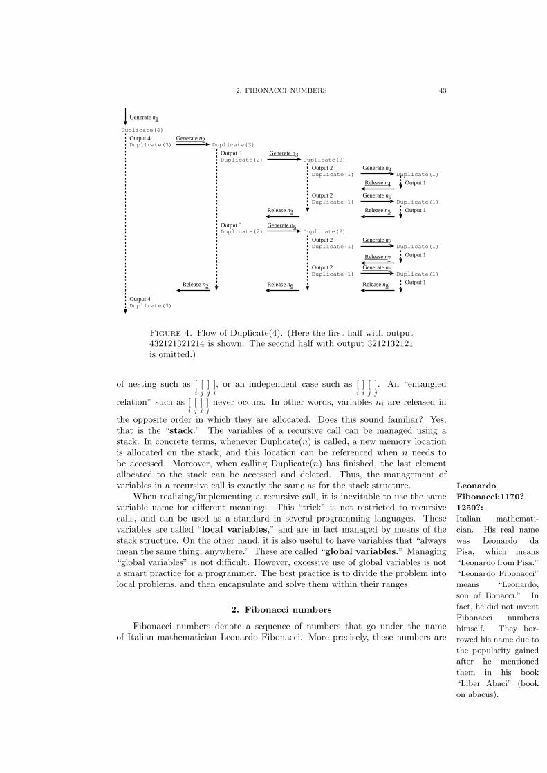
2. FIBONACCI NUMBERS 43

Duplicate(4)

Output 4Duplicate(3)

Output 4Duplicate(3)

Duplicate(3)

Output 3Duplicate(2)

Output 3Duplicate(2)

Duplicate(2)

Output 2Duplicate(1)

Output 2Duplicate(1)

Duplicate(1)

Output 1

Duplicate(1)

Output 1

Duplicate(2)

Output 2Duplicate(1)

Output 2Duplicate(1)

Duplicate(1)

Output 1

Duplicate(1)

Output 1

Generate n1

Generate n2

Release n2

Generate n3

Release n3

Generate n4

Release n4

Generate n5

Release n5

Generate n6

Release n6

Generate n7

Release n7

Generate n8

Release n8

Figure 4. Flow of Duplicate(4). (Here the first half with output432121321214 is shown. The second half with output 3212132121is omitted.)

of nesting such as [i

[j

]j

]i

, or an independent case such as [i

]i

[j

]j

. An “entangled

relation” such as [i

[j

]i

]j

never occurs. In other words, variables ni are released in

the opposite order in which they are allocated. Does this sound familiar? Yes,that is the “stack.” The variables of a recursive call can be managed using astack. In concrete terms, whenever Duplicate(n) is called, a new memory locationis allocated on the stack, and this location can be referenced when n needs tobe accessed. Moreover, when calling Duplicate(n) has finished, the last elementallocated to the stack can be accessed and deleted. Thus, the management ofvariables in a recursive call is exactly the same as for the stack structure. Leonardo

Fibonacci:1170?–

1250?:

Italian mathemati-

cian. His real name

was Leonardo da

Pisa, which means

“Leonardo from Pisa.”

“Leonardo Fibonacci”

means “Leonardo,

son of Bonacci.” In

fact, he did not invent

Fibonacci numbers

himself. They bor-

rowed his name due to

the popularity gained

after he mentioned

them in his book

“Liber Abaci” (book

on abacus).

When realizing/implementing a recursive call, it is inevitable to use the samevariable name for different meanings. This “trick” is not restricted to recursivecalls, and can be used as a standard in several programming languages. Thesevariables are called “local variables,” and are in fact managed by means of thestack structure. On the other hand, it is also useful to have variables that “alwaysmean the same thing, anywhere.” These are called “global variables.” Managing“global variables” is not difficult. However, excessive use of global variables is nota smart practice for a programmer. The best practice is to divide the problem intolocal problems, and then encapsulate and solve them within their ranges.

2. Fibonacci numbers

Fibonacci numbers denote a sequence of numbers that go under the nameof Italian mathematician Leonardo Fibonacci. More precisely, these numbers are

44 2. RECURSIVE CALL

known as Fibonacci sequence, and the numbers that belong to this are called Fi-bonacci numbers. The sequence actually has quite a simple definition, namely:

F (1) = 1,

F (2) = 1,

F (n) = F (n− 1) + F (n− 2) (for n > 2).

In concrete terms, the sequence can be enumerated as 1, 1, 2, 3, 5, 8, 13, 21, 34, 55, 89, . . ..The Fibonacci sequence F (n) is known to attract widespread interest for frequentlyappearing as a numerical model when we try to build models representing naturalphenomena, such as the arrangement of seeds in sunflowers, the number of rabbitsiblings, and others. Let us deepen our understanding of recursive calls using thissequence. At the same time, let us discover the limitations of recursive calls andintroduce further refinements.

2.1. Computing Fibonacci numbers F (n) arising from recursive calls.There is one particular aspect that must be considered carefully when workingwith recursive calls. We have seen that, in recursive calls, the algorithm capableof solving its own partial problem is reused. It is worth noting to what extentthis “partial problem” is necessary. In the Tower of Hanoi problem, we reused thealgorithm for solving the partial problem of size n− 1 to solve a problem of size n.Considering the definition of Fibonacci numbers F (n), the values of both F (n− 1)and F (n− 2) are required. From this fact, we learn that it does not suffice to showa clear solution for the small partial problem in n = 1, but the solutions for n = 1and n = 2 are also needed. If we construct the algorithm according to its definitionwhile paying attention to this point, we obtain the algorithm below. Using thisalgorithm, the n-th Fibonacci number F (n) can be obtained by calling Fibr(n),which produces the returned value as its output.

Algorithm 13：recursive algorithm Fibr(n) to compute the n-th Fibonaccinumber F (n)

Input ：nOutput ：the n-th Fibonacci number F (n)

1 if n = 1 then return 1;

2 if n = 2 then return 1;

3 return Fibr(n− 1) + Fibr(n− 2);

Exercise 20. Implement and execute the algorithm above. How willthe program behave when n is made slightly larger (by a few tens)?

2.2. Execution time of Fibr based on recursive calls. When we imple-ment and execute Fibr(n), execution clearly slows down for values around n = 40and above. Why does this occur? Let us consider an execution time tF (n). Whenconsidering execution times, examining the recursive equation is inevitable. Inconcrete terms, we have:

• For n = 1: a constant time tF (1) = c1

• For n = 2: a constant time tF (2) = c2

• For n > 2: for a given constant c3, tF (n) = tF (n− 1) + tF (n− 2) + c3

Here, the value of the constant itself has no meaning, and therefore we can simplydenote them as c. By adding c to both sides of the equation, for n > 2 we can

2. FIBONACCI NUMBERS 45

F(9) F(8) F(7) F(6) F(5) F(4) F(3) F(2)

F(1)F(2)

F(3) F(2)

F(1)F(4) F(3) F(2)

F(1)F(2)

F(5) F(4) F(3) F(2)

F(1)F(2)

F(3) F(2)

F(1)F(6) F(5) F(4) F(3) F(2)

F(1)F(2)

F(3) F(2)

F(1)F(4) F(3) F(2)

F(1)F(2)

F(7) F(6) F(5) F(4) F(3) F(2)

F(1)F(2)

F(3) F(2)

F(1)F(4) F(3) F(2)

F(1)F(2)

F(5) F(4) F(3) F(2)

F(1)F(2)

F(3) F(2)

F(1)

Figure 5. Aspect of the computation of the Fibonacci number F (9)

write:tF (n) + c = (tF (n− 1) + c) + (tF (n− 2) + c)

In other words, if we introduce another function t′F (n) = tF (n) + c, we can write:

t′F (n) = t′F (n− 1) + t′F (n− 2),

which is exactly equivalent to the definition of Fibonacci numbers. In other words,the execution time tF (n) of Fibr(n) can be considered proportional to the valueof Fibonacci numbers. If we anticipate the contents of Section 2.4 below, it isknown that Fibonacci numbers F (n) will be F (n) ∼ Θ(1.618n). In other words,Fibonacci numbers constitute an exponential function. Therefore, if we computeFibonacci numbers according to their definition, the computation time tends toincrease exponentially, that is, if n becomes larger, the computation time of a naıveimplementation is excessively large.

2.3. Fast method for computing Fibonacci numbers. We learned that,according to the definition, the time required to compute Fibonacci numbers in-creases exponentially. However, some readers may feel intrigued by that. For in-stance, to compute F (9), only F (8) to F (1) suffice. First, let us solve the questionwhy the time required for computing Fibonacci numbers increases exponentially.For example, F (9) can be computed if F (8) and F (7) are available. ComputingF (8) only requires knowing F (7) and F (6), and computing F (7) only requires F (6)and F (5), and so forth. This calling mechanism is illustrated in Figure 5.

46 2. RECURSIVE CALL

What we need to note here is “who is calling who.” For instance, if we payattention to F (7), this value is called twice, that is, upon the computation of bothF (9) and F (8). That is, F (7) is nested twice to compute F (9). Likewise, F (6) iscalled from F (8) and F (7), and F (7) is called twice. This structure becomes moreevident as we approach the leaves of the tree structure. F (2) and F (3) appear inFigure 5 remarkably often. Thus, the Fibr(n) algorithm based on recursive callscomputes the same value over and over again in a wasteful fashion.

Once the problem becomes clear at this level, the solution naturally becomesevident. The first idea that pops up is to use arrays. Using an array, we canstart computing from the smallest value and refer to this value when necessary.Concretely speaking, we can use the following algorithm:

Algorithm 14：Algorithm Fiba(n) to compute the n-th Fibonacci numberF (n) using array Fa[]

Input ：nOutput ：n-th Fibonacci number F (n)

1 Fa[1]←1;

2 Fa[2]←1;

3 for i← 3, 4, . . . , n do4 Fa[i]← Fa[i− 1] + Fa[i− 2];

5 end

6 output Fa[n];

First, F (1) and F (2) are directly computed when i = 1, 2. Then, for i > 2 it isquite clear that for computing Fa[i] we already have the correct values of Fa[i− 1]and Fa[i − 2]. These two observations indicate to us that Fibonacci numbers canbe correctly computed by this algorithm. Therefore, the computation time of theFiba(n) algorithm is linear, that is, proportional to n, which means it is extremelyfast.

Let us stop for a while to think ahead. For i > 2, what is necessary forcomputing F (i) is F (i − 1) and F (i − 2), and elements further behind are notneeded. In other words, provided that we keep in mind the last two elements, thearray itself is unnecessary. With that perception in mind, we can write an evenmore efficient algorithm (from the viewpoint of memory space):

2. FIBONACCI NUMBERS 47

Algorithm 15：Algorithm Fib2(n) to compute the n-th Fibonacci numberF (n) without using arrays

Input ：nOutput ：n-th Fibonacci number F (n)

1 if n < 3 then2 output “1”;

3 else4 Fa1← 1 ; /* Memorize F (1) */

5 Fa2← 1 ; /* Memorize F (2) */

6 for i← 3, 4, . . . , n do7 Fa← Fa2 + Fa1 ; /* Compute/memorize F (i) = F (i− 1) + F (i− 2) */

8 Fa1← Fa2 ; /* Update F (i− 2) with F (i− 1) */

9 Fa2← Fa ; /* Update F (i− 1) with F (i) */

10 end

11 output Fa;

12 end

Exercise 21. Implement and execute the algorithm above. Confirmthat the answer is output immediately even for very large values of n.

2.4. Extremely fast method to compute Fibonacci numbers. Fibonaccinumbers F (n) have fascinated mathematicians since ancient times due to their in-triguing and interesting properties. In this section, let us borrow some of the resultsof such mathematical research. In fact, it is known that the general term of Fi-bonacci numbers F (n) can be expressed by the following expression:

F (n) =1√5

((1 +√

52

)n

−

(1−√

52

)n)

It is fascinating that even though√

5 appears several times in the equation, theresult F (n) is always a natural number for any input n that is a natural number. Ifwe implement an algorithm that computes this equation, the computation time ofa Fibonacci number F (n) ends in a constant time. (Considering the errors involvedin the computation of

√5, there might be cases in which the algorithm that allows

computation in linear time of the previous section is preferable.)In the present Section, let us prove that the Fibonacci number F (n) approxi-

mately follows Θ(1.618n). First, consider the two terms(

1+√

52

)n

and(

1−√

52

)n

.

If we actually compute them, we obtain(

1+√

52

)= 1.61803 . . . and

(1−

√5

2

)=

−0.61803 . . .. Thus, the absolute value of the former is considerably larger than1, whereas the absolute value of the latter is considerably smaller than 1. There-fore, as n increases the value of

(1+

√5

2

)n

increases very fast, whereas the value of(1−

√5

2

)n

becomes small very quickly. Thus, the value of F (n) is approximately

1.618n/√

5, which is of the order Θ(1.618n), i.e., an exponential function.

Exercise 22. Prove by means of mathematical induction that thegeneral term equation for Fibonacci numbers F (n) actually holds.

48 2. RECURSIVE CALL

Exercise 23. Investigate the relation between Fibonacci numbersF (n) and the golden ratio φ. The golden ratio φ is a constant defined as φ =1+

√5

2 , and its value is approximately 1.618.

3. Divide-and-conquer and dynamic programming

When tackling a large problem using a computer, approaching the problemdirectly as a whole often does not lead to good results. In such cases, we mustfirst consider whether it is possible to split the large problem into small partialproblems. In many cases, a large problem that cannot be tackled as it is can besplit into sufficiently small partial problems that can be appropriately handled in-dividually. Solving these individual partial problems and combining their solutionsoften permits the original large problem to be solved. This method is known as“divide and conquer.” The idea is that a large target must be divided to allowfor proper management. Political units such as countries, prefectures, cities, towns,and villages also constitute examples of this idea. The divide-and-conquer methodcan be considered a “top-down” approach.

The Tower of Hanoi problem was successfully solved by splitting the originalproblem consisting of moving n discs into the following partial problems:

• Partial problem where the number of discs is n− 1• Partial problem of moving only 1 disc (the largest one)

This is an example of divide-and-conquer. Regarding the computation of Fibonaccinumbers, using a recursive definition for computation can be considered a divide-and-conquer method. However, in the case of Fibonacci numbers, we found a com-putation method that is much more efficient than the divide-and-conquer method.The limitation of the “divide-and-conquer” method for Fibonacci numbers is thatthe solution to the problems that had already been solved is forgotten every time.This is a characteristic of top-down approaches that is difficult to avoid, a fatal lim-itation in the case of Fibonacci numbers. This condition resembles the situation ofvertical administration systems where similar organizations exist in several places.

Dynamic programming is a method conceived to address such problems. Inthis method, minutely sliced problems are solved in a bottom-up approach. Whenoptimal solutions to partial problems are found, such that no further improvementis possible, only the necessary information is retained and all the unnecessary infor-mation is forgotten. In the Fibonacci numbers example, an important point is thatcomputations are carried out in a determined order, starting from the small values.Because only the values of the Fibonacci numbers immediately preceding F (i− 1)and F (i− 2) are needed, values further back can be forgotten. In other words, forFibonacci number computation, it suffices to retain only the previous two values.

In the case of the Tower of Hanoi problem, because all discs must be movedevery time, the problem does not fit well in the dynamic programming framework.For this reason, the solution is limited to the divide-and-conquer method.

CHAPTER 3

Algorithms for Searching and Sorting

bababababababababababababababab

Searching and sorting are two basic problems that contain many valuableelements for algorithms. They are still being investigated in many relatedareas. The series of books entitled “The Art of Computer Programming”by D. E. Knuth is said to be “the bible” of algorithmic theory, and thethird volume has the subtitle “Sorting and Searching.” We will enjoy andunderstand these deep problems in this chapter.

Donald Ervin

Knuth (1938–):

He is a professor

emeritus of computer

science at Stanford

University. The series

of books mentioned

in the text is called

“TAOCP.” It was

planned to publish

the series in seven

volumes, starting in

the 1960s. Now, some

preliminary drafts of

the fourth volume are

public on the Web.

It is surprising that,

to write this series,

Knuth first started

with designing and

programming the

well-known TEX sys-

tem for typesetting,

and the METAFONT

system for designing

typesetting fonts. See

Chapter 7 for more

details.

What you will learn: • Linear search• Sentinel• Block search• Binary search• Lower bound for searching• Hash• Bubble sort• Merge sort• Quick sort• Lower bound for sorting• Bucket sort• Spaghetti sort

49

50 3. ALGORITHMS FOR SEARCHING AND SORTING

1. Searching

We first consider the search problem that is formalized as

Searching:

Input: An array a[1], a[2], . . . , a[n] and data x.Output: The index i such that a[i] = x.

There are some variants of the problem according to the conditions, e.g.,• It is guaranteed that there exists an i such that a[i] = x for every x or

not.• The array a[] may contain the same data two or more times, that is,

a[i] = a[j] for some i 6= j or not.• The elements in a[] are preprocessed following some rule or not. One typ-

ical assumption is that a[1] ≤ a[2] ≤ a[3] ≤ · · · ≤ a[n]. In real data, suchas dictionaries and address books, in general, massive data are organizedin some order.

For the moment, we have no special assumption on the ordering of data.

1.1. Linear search and its running time. A natural straightforward searchmethod is the linear search; it checks the data from a[1] to the last data item oruntil finding x. The algorithm’s description is simple:

Algorithm 16：LinearSearch(a, x)Input ：An array a[] and data xOutput ：The index i if there is an i with a[i] = x; otherwise, “Not found.”

1 i← 1;

2 while i ≤ n and a[i] 6= x do3 i← i + 1;

4 end

5 if i ≤ n then6 output i;

7 else8 output “Not found”;

9 end

We now explain the while statement, which appears here for the first time. Thewhile statement is one of the control statements. It means “repeating some state-ments while given condition.” In this linear search, after initializing the variable iby 1 at line 1, the statement “i ← i + 1” is repeated while the condition “i ≤ nand a[i] 6= x” holds. In other words, when we have “i > n or a[i] = x,” the loophalts and the program goes to the next step. If we look at the manner in which thewhile statement works, the correctness of the algorithm is easy to see. The runningtime is Θ(n), which is also easily seen. When there is no i such that a[i] = x, thealgorithm halts in Θ(n) time, and if there is an i with a[i] = x, the algorithm findsit after checking n/2 elements in the average case. (Of course, this “average case”depends on the distribution of the data.)

Sentinel. We now introduce a useful technique for linear searching. This technique,which is a type of programming technique rather than an algorithmic one, is called

1. SEARCHING 51

sentinel. One may feel that the linear search algorithm described above is a bitmore complicated than necessary. The reason is that, in the while statement, wesimultaneously check two essentially different conditions:

• Whether the array a[i] ends or not, and• Whether i satisfies a[i] = x or not.

Moreover, although the algorithm checks whether i ≤ n in line 5, this check has al-ready been performed once in the last while statement. This seems to be redundant.Although the basic idea of the algorithm is simple, and even though the idea of theunderlying algorithm is also simple, when we consider the boundary conditions inthe implementation, it becomes complicated. This is often the case. How can weresolve it?

One of the techniques for resolving this complexity is called sentinel. This isa neat idea for unifying these two conditions “check the end of the array a[]” and“check the index i with a[i] = x.” To apply this idea, we first prepare an additionalelement a[n + 1] and initialize it by x. Then, of course, there does exist an index iwith a[i] = x in the interval 1 ≤ i ≤ n + 1. In this case, we find i with a[i] = x inthe original array if and only if 1 ≤ i ≤ n. Therefore, the algorithm can decide tooutput i only if i < n + 1. This element a[i + 1] is called the sentinel. Using thistechnique, the algorithm can be rewritten in a smarter style.

Algorithm 17：LinearSearchSentinel(a, x)Input ：An array a[] and data xOutput ：The index i if there is an i with a[i] = x; otherwise, “Not found.”

1 i← 1;

2 a[n + 1]← x; ; /* This is the sentinel. */

3 while a[i] 6= x do4 i← i + 1;

5 end

6 if i < n + 1 then7 output i;

8 else9 output “Not found”;

10 end

It may seem a trifling improvement, but the conditions in while are checkedevery time, and this 50% reduction is unexpectedly efficient. Although it can beapplied only if we can use an additional element in the array, it is a noteworthytechnique.

1.2. Searching in pre-sorted data. In the linear search method, we assumenothing about the ordering of the data. Thus, we cannot guess where x can be inthe array at all. In this case, we have a few tricks for improving the linear searchmethod, but it seems to be impossible to achieve a better running time than Θ(n).Now, we turn to the significant case where the data are ordered. That is, our nextproblem is the following.

Searching in ordered data:

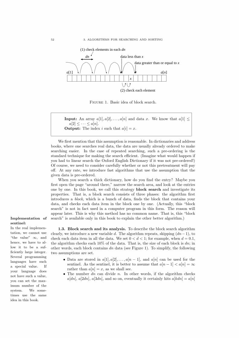
52 3. ALGORITHMS FOR SEARCHING AND SORTING

a[1] a[n]

dn

x

data less than x

data greater than or equal to x

(1) check elements in each dn

(2) check each element

Figure 1. Basic idea of block search.

Input: An array a[1], a[2], . . . , a[n] and data x. We know that a[1] ≤a[2] ≤ · · · ≤ a[n].

Output: The index i such that a[i] = x.

We first mention that this assumption is reasonable. In dictionaries and addressbooks, where one searches real data, the data are usually already ordered to makesearching easier. In the case of repeated searching, such a pre-ordering is thestandard technique for making the search efficient. (Imagine what would happen ifyou had to linear search the Oxford English Dictionary if it was not pre-ordered!)Of course, we need to consider carefully whether or not this pretreatment will payoff. At any rate, we introduce fast algorithms that use the assumption that thegiven data is pre-ordered.

When you search a thick dictionary, how do you find the entry? Maybe youfirst open the page “around there,” narrow the search area, and look at the entriesone by one. In this book, we call this strategy block search and investigate itsproperties. That is, a block search consists of three phases: the algorithm firstintroduces a block, which is a bunch of data, finds the block that contains yourdata, and checks each data item in the block one by one. (Actually, this “blocksearch” is not in fact used in a computer program in this form. The reason willappear later. This is why this method has no common name. That is, this “blocksearch” is available only in this book to explain the other better algorithm.)Implementation of

sentinel:

In the real implemen-

tation, we cannot use

“the value” ∞, and

hence, we have to al-

low it to be a suf-

ficiently large integer.

Several programming

languages have such

a special value. If

your language does

not have such a value,

you can set the max-

imum number of the

system. We some-

times use the same

idea in this book.

1.3. Block search and its analysis. To describe the block search algorithmclearly, we introduce a new variable d. The algorithm repeats, skipping (dn−1), tocheck each data item in all the data. We set 0 < d < 1; for example, when d = 0.1,the algorithm checks each 10% of the data. That is, the size of each block is dn; inother words, each block contains dn data (see Figure 1). To simplify, the followingtwo assumptions are set.

• Data are stored in a[1], a[2], . . . , a[n − 1], and a[n] can be used for thesentinel. As the sentinel, it is better to assume that a[n− 1] < a[n] =∞rather than a[n] = x, as we shall see.• The number dn can divide n. In other words, if the algorithm checks

a[dn], a[2dn], a[3dn], and so on, eventually it certainly hits a[kdn] = a[n]

1. SEARCHING 53

for some integer k, and compares x with a[n], the sentinel, and obtainsx < a[n].

Based on the assumptions, the algorithm can be described as follows.

Algorithm 18：BlockSearch(a, x)Input ：An ordered array a[1], a[2], . . . , a[n] and data xOutput ：The index i if there is an i with a[i] = x; otherwise, “Not found.”

1 i← dn;

2 while a[i] < x do3 i← i + dn;

4 end

/* We can assert that a[i− dn] < x ≤ a[i] holds at this point. */

5 i← i− dn + 1;

6 while a[i] < x do7 i← i + 1;

8 end

9 if a[i] = x then10 output i;

11 else12 output “Not found”;

13 end

In the while loop from line 2 to 4, the algorithm searches the smallest index iwith a[i] ≥ x for each dn data item. Therefore, when it exits this while loop, wehave a[i− dn] < x ≤ a[i]. Since x can exist from a[i− dn + 1] to a[i], the algorithmchecks whether x exists in the data elements in this interval from a[i− dn + 1] oneby one in the while loop from lines 6 to 8. (We can skip the (i − dn)th element,because we already know that a[i− dn] < x.) When the while loop from line 6 to 8is complete, we know that x ≥ a[i]. This time, in line 9, we can determine whethera[i] contains x for some i with i itself by checking whether x = a[i] or not. Byvirtue of the sentinel a[n] =∞, it is guaranteed that there exists an i that satisfiesx < a[i], which makes the second while loop simple.

Now, we estimate the running time of block search and compare it with thatof linear search. How about the first narrowing step? In the worst case, the searchchecks n/(dn) = 1/d elements in the array a[i] for each dn element. In the averagecase, we can consider the running time to be 1/(2d). The next step is essentiallythe same as in a linear search. However, this time we have only dn data. Therefore,it runs in dn time in the worst case and dn/2 in the average case. Summing up,the algorithm runs in Θ(1/d + dn) time in both the worst and average case. If welet d be larger, the time of the steps in the former half decreases, but that in thelatter half increases. On the other hand, when d is set smaller, the algorithm runsmore slowly in the former half. With careful analysis, these two factors becomewell-balanced when d = 1/

√n, and then, the running time becomes Θ(

√n), which

is the minimum.

Exercise 24. Explain that for the function Θ(1/d + dn), d = 1/√

ngives us the minimum function Θ(

√n).

Recalling that the linear search runs in Θ(n), it can be seen that the runningtime Θ(

√n) is a great improvement. For example, when n = 1000000, the block

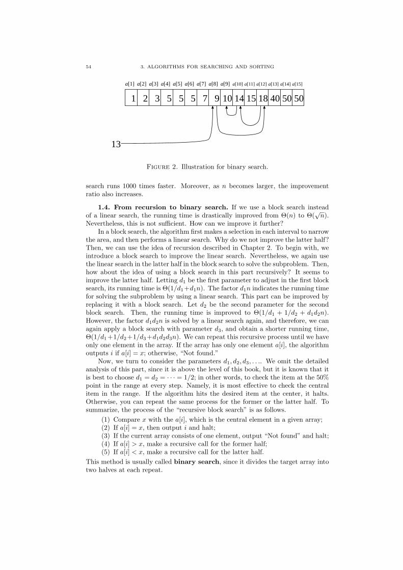
54 3. ALGORITHMS FOR SEARCHING AND SORTING

1 2 3 5 5 5 7 9 10 14 15 18 40 50 50

a[1] a[2] a[3] a[4] a[5] a[6] a[7] a[8] a[9] a[10] a[11] a[12] a[13] a[14] a[15]

13

Figure 2. Illustration for binary search.

search runs 1000 times faster. Moreover, as n becomes larger, the improvementratio also increases.

1.4. From recursion to binary search. If we use a block search insteadof a linear search, the running time is drastically improved from Θ(n) to Θ(

√n).

Nevertheless, this is not sufficient. How can we improve it further?In a block search, the algorithm first makes a selection in each interval to narrow

the area, and then performs a linear search. Why do we not improve the latter half?Then, we can use the idea of recursion described in Chapter 2. To begin with, weintroduce a block search to improve the linear search. Nevertheless, we again usethe linear search in the latter half in the block search to solve the subproblem. Then,how about the idea of using a block search in this part recursively? It seems toimprove the latter half. Letting d1 be the first parameter to adjust in the first blocksearch, its running time is Θ(1/d1+d1n). The factor d1n indicates the running timefor solving the subproblem by using a linear search. This part can be improved byreplacing it with a block search. Let d2 be the second parameter for the secondblock search. Then, the running time is improved to Θ(1/d1 + 1/d2 + d1d2n).However, the factor d1d2n is solved by a linear search again, and therefore, we canagain apply a block search with parameter d3, and obtain a shorter running time,Θ(1/d1+1/d2+1/d3+d1d2d3n). We can repeat this recursive process until we haveonly one element in the array. If the array has only one element a[i], the algorithmoutputs i if a[i] = x; otherwise, “Not found.”

Now, we turn to consider the parameters d1, d2, d3, . . .. We omit the detailedanalysis of this part, since it is above the level of this book, but it is known that itis best to choose d1 = d2 = · · · = 1/2; in other words, to check the item at the 50%point in the range at every step. Namely, it is most effective to check the centralitem in the range. If the algorithm hits the desired item at the center, it halts.Otherwise, you can repeat the same process for the former or the latter half. Tosummarize, the process of the “recursive block search” is as follows.

(1) Compare x with the a[i], which is the central element in a given array;(2) If a[i] = x, then output i and halt;(3) If the current array consists of one element, output “Not found” and halt;(4) If a[i] > x, make a recursive call for the former half;(5) If a[i] < x, make a recursive call for the latter half.

This method is usually called binary search, since it divides the target array intotwo halves at each repeat.

1. SEARCHING 55

Example 5. For the array given in Figure 2, let us perform a binary searchwith x = 13. The number of elements in a[] is 15; thus, we check whether a[8] = 9is equal to x = 13 or not. Then, we have x > a[8]. Thus, the next range ofthe search is a[9], . . . , a[15]. Here, we have seven elements; therefore, we checkwhether a[12] = 18 is equal to x, and obtain a[12] > x. Thus, the range is nowa[9], a[10], a[11]. Comparing a[10] = 14 to x = 13, we have a[10] > x. Next, wecheck a[9] = 10 and x = 13 and conclude that the array a[] does not contain x as adata item.

Exercise 25. Implement a binary search on your computer.

Now, we consider the running time of the binary search method. The essenceof the running time is the number of comparisons. Therefore, we here simplifythe analysis and investigate only the number of comparisons. (The entire runningtime is proportional to the number of comparisons; it is essentially the same asconsidering it by using the O-notation.) The algorithm halts if it finds a[i] = x forsome i; however, we consider the worst case, that is, the algorithm checks the lastelement and outputs “Not found.” In this case, the range of the array is halvedin each comparison and the algorithm halts after checking the last element in thearray of size 1. Therefore, the number of comparisons TB(n) in the binary searchon an array of size n satisfies the relations

TB(n) = 1 (if n = 1)TB(n) = TB(d(n− 1)/2e) + 1 (if n > 1),

where d(n− 1)/2e denotes the minimum integer greater than or equal to (n− 1)/2.In general, the algorithm picks up one data element from n data, compares it, anddivides the remaining (n−1) elements. In this case, if n−1 is even we have (n−1)/2elements, but we still have n/2 in the worst case (or a larger range) if n− 1 is odd.Since such details are not essential, we simplify the equations as

T ′B(n) = 1 (if n = 1)

T ′B(n) = T ′

B(n/2) + 1 (if n > 1).

Moreover, we assume that n = 2k. Then, we have

TB(2k) = TB(2k−1) + 1 = TB(2k−2) + 2 = · · · = TB(1) + k = 1 + k.

From n = 2k, we obtain k = log n. In general, if n cannot be represented in 2k

for an integer k, we may add imaginary data and consider the minimum n′ suchthat n < n′ = 2k for some integer k. In this case, we can analyze for n′ and applythe analysis results to the smaller n. From these arguments, we have the followingtheorem.

Theorem 6. The binary search on n data runs in O(log n) time.

As emphasized in the logarithmic function in Section 5, the function in O(log n)is quite small and the binary search runs quite fast. In comparison to the originaltime Θ(n) for linear search, it may be said to be “almost constant time.” For exam-ple, the population of Japan is around 120,000,000 and log 120000000 = 26.8385.That is, if you have a telephone book that contains the entire Japanese population,you can reach any person in at most 27 checks. If you use a linear search, the num-ber of checks is still 120,000,000, and even the block search of O(

√n) also requires

checking√

12000000 ∼ 11000 times. Therefore, 27 is notably smaller.

56 3. ALGORITHMS FOR SEARCHING AND SORTING

Exercise 26. The largest Japanese dictionary consists of around 240,000words. If you use a binary search, how many words need to be checked to find aword in the worst case?

We have considered the linear, block, and binary search methods. One maythink that the binary search method, as an improvement on the block searchmethod, is complicated. However, the binary search algorithm is indeed simple.Therefore, the implementation is easy, and it is in fact quite a fast algorithm. Forthis reason, the block search method is not used in practice.

Lower bound of searching. The binary search method is a simple and fastalgorithm. In fact, it is the best algorithm and cannot be improved further fromthe theoretical viewpoint. More precisely, the following theorem is known.

Theorem 7. Let A be any algorithm that searches by comparing a pair of dataitems. If A can use fewer than log n comparison operations, the search problem forn data cannot be solved by A.

To give a strict proof, we have to borrow some notions from information theory.However, intuitively, it is not very difficult to understand. As seen in the RAMmodel in Section 1, to store n different data in a memory cell and give them uniqueaddresses (or indices), each address requires log n bits. This fact implies that, toResults of a com-

parison:

Here, to simplify, we

assume that x < y

or x > y holds in

a comparison. We

omit the other possi-

ble case, x = y, in

this book. Another

issue is that log n is

not an integer in gen-

eral. To be precise,

we have to take dlog neor blog nc according to

the context, which is

also omitted in this

book.

distinguish n data, log n bits are necessary. On the other hand, when we comparetwo data items, we obtain 1 bit information about their ordering. Therefore, tospecify the position of x in the array a[] of n elements, we need to make log ncomparisons to obtain that log n bit address. In other words, if some algorithmuses only fewer than log n comparisons, we can make counter data to the algorithm.For this counter data, the algorithm will leave two or more data that should becompared with x.

2. Hashing

In Theorem 7, we show the lower bound log n comparisons to solve the searchingif the algorithm uses comparison as a basic operator. If you sense something strangeabout the basic operation, you are clever. Indeed, sometimes we can break this limitby using another technique not based on comparison. The hash is one of them.We first observe a simple hash to understand the idea.

Simple hash. The search problem asks whether there is an index i with a[i] = xfor a given array a[1], a[2], . . . , a[n] and data x. We here assume that we knowbeforehand that “x is an integer between 1 and n.” For example, most studentexamination scores are between 1 and 100; hence, this assumption is a simple butrealistic one. The array a[i] indicates whether there is a student whose score is i.To represent this, we define that a[i] = 0 means “there is no data item of valuei” and a[i] = i if “there is a data item of value i” and the array is supposed tobe initialized following the definition. Then, for a given x, we can solve the searchproblem in O(1) time by checking whether a[x] = x.

Idea of general Hash. Now, we turn to general hash. In general, there is nolimitation on the range of x. Thus, x can be much larger than n. How can we dealwith such a case? The answer to this question is the notion of the hash function.The hash function h(x) should satisfy two conditions:

(1) The function h(x) takes an integer in the area [1..n].

2. HASHING 57

(2) If x is in the array a[], it is stored as in a[h(x)].If we already know that the data in the array a[] and a function h satisfy theseconditions, the idea of hash can be described in algorithmic form as

Algorithm 19：Hash(a, x)Input ：An array a[1], a[2], . . . , a[n] and data xOutput ：The index i if there is an i with a[i] = x; otherwise, “Not found.”

1 if a[h(x)] = x then2 output h(x);

3 else4 output “Not found”;

5 end

Since it is quite simple, it is easy to see that the algorithm certainly finds x ifit exists, and its running time is O(1). In short, the function h(x) computes theindex of x in the array a[]. Thus, if the function h(x) is correctly implemented, thesearching problem can be solved efficiently. In the notion of hash, x is called a keyand h(x) is called the hash value for the key x.

Implementation of hash function. As we have already seen, to perform thehash function correctly its implementation is crucial. Unfortunately, we have nosilver bullet for designing a universal hash function. The difficulty is in satisfyingthe second condition. To achieve this

(3) For any pair x and x′, we have to guarantee that x 6= x′ implies h(x) 6=h(x′).

Otherwise, for some two different keys x and x′, we will refer to the same dataa[h(x)] = a[h(x′)]. In the general case, or when there is no limit to the key, wecannot guarantee this condition. That is, even if we design a “nice” hash function,we can say at most that

(3’) For h(x), we have few x′ with x 6= x′ such that h(x) = h(x′).A case where “x 6= x′ and h(x) = h(x′)” is called a collision of the hash value.When you use a hash function, you have to create a design that avoids collisions asfar as possible, and you have to handle collisions. Hereafter, we introduce the designtechnique for hash functions and the manner in which can we handle collisions. Thisbook introduces only a few typical and simple techniques, but there are many othersfor handling collisions.

Typical hash function. When x takes an integer, we have to map to an integerin [1..n], and the most simple hash function is “(x modulo n) + 1.” If x can bebiased, choosing suitable integers a and b beforehand, we take “((ax + b) modulon) + 1.” Experimentally, it behaves well when you take a, b and n relatively primeto each other. If x is not an integer, we can use its binary representation in thecomputer system as a binary number, and handle in the same way.

Avoiding collision. For a given key x, assume that it occurs that a[h(x)] = x′

with x 6= x′, that is, we have a collision. In this case, a simple solution is to prepareanother function to indicate “the next position” for x. Among these techniques,the simplest is to let “the next position” be the next empty element in a[]. Thatis, algorithmically, it is described as

(1) Let i = 0.

58 3. ALGORITHMS FOR SEARCHING AND SORTING

(2) For a given key x, check a[h(x)+ i], and report h(x)+ i if a[h(x)+ i] = x.(3) If a[h(x) + i] is empty, report “Not found.”(4) Otherwise, if a[h(x) + i] = x′ for some x′ with x′ 6= x, increment i (or

perform i← i + 1), and go to step 2.The implementation is easy and it runs efficiently if few collisions occur.

Caution for usage. If you can use the hash function correctly, your algorithmruns fast. If no or few collisions occur, the search can be complete in O(1) time.Therefore, the crucial point is to design the hash function h(x) such that a few orfewer collisions occur. To achieve this, the density of the data in a[] is one of theissues. In a general search problem, sometimes new data are added, and useless dataare removed. Therefore, not all the elements in a[] are necessarily valid. Rather, ifa[] contains few data, few collisions occur, even if you use a simple hash function.In contrast, if most of a[] are used to store data, collisions frequently occur and thetime required for the computation to avoid collisions becomes an issue. Since theavoiding method introduced above essentially performs a linear search, if collisionsoccur frequently, we have to refine this process. There are many tricks for handlingthis problem according to the size of the memory and the number of data; however,we omit them in this book.

3. Sorting

Next, we turn to the sorting problem. As seen in the binary search, if thearray is organized beforehand, we can search quite efficiently. If all the items inyour dictionary are incoherently ordered, you cannot find any word. Thus, you canunderstand that huge data are meaningful only if the entries are in order. Therefore,the following sorting problem is important in practice.

Sorting:

Input: Array a[1], a[2], . . . , a[n].Output: Array a[1], a[2], . . . , a[n], such that a[1] ≤ a[2] ≤ · · · ≤ a[n]

holds.

We first mention two points that should be considered when handling the sort-ing problem.

First, it is required that in the array the ordering of each pair is defined cor-rectly. (Using a technical term, we can say that we have “total ordering” over thedata.) For example, in the game of “paper, rock, scissors,” we have three choicesand each pair has an ordering. However, they are not in total ordering, and hence,we cannot sort them. More precisely, the data should have the following properties.(1) For each pair of x and y, we have x < y or x > y, and (2) For each triple ofx, y, and z, x < y and y < z implies x < z. In other words, once we know x < yand y < z, we can conclude x < z without comparing them. Oppositely, not onlynumerical data, but also other data can be sorted if total ordering is defined overthe data. Typically, we can sort alphabetical words as in a dictionary.

Second, in sorting, if the data contain two or more items with the same value,we have to be careful. Depending on the sorting algorithm, the behavior differsfor two items of the same value. For example, when we have two items a[i] = a[j]with i < j, the sorting algorithm is called stable if the ordering of a[i] and a[j] is

3. SORTING 59

always retained in the output. If we are dealing with only numerical data, even ifthe items are swapped, we are not concerned. However, the target of sorting maynot be only numerical data. Sometimes the bunch of data consists of some indicesof complicated data. For example, imagine that you have a huge amount of dataconsisting of responses to a questionnaire, and you wish to sort them by the namesof the responders. In this case, it is not good if the attributes of two people of thesame name are swapped. Thus, the stability of sorting can be an issue in someapplications.

3.1. Bubble sort. One of the simplest sorting techniques is called bubblesort. The basic idea is natural and simple: compare two consecutive items, swapthem if they are in reverse order, and repeat. Now we explain in more detail. Thealgorithm first performs the following step.

• For each i = 1, 2, . . . , n − 1, compare a[i] and a[i + 1], and swap them ifa[i] > a[i + 1].

The important point is that after this step, the biggest item is put into a[n]. It isnot difficult to observe this fact since the algorithm swaps from a[1] to a[n − 1].Once the algorithm has hit the biggest item, this item is always compared with thenext item, one by one, and eventually is moved to a[n]. Then, we can use the samealgorithm for the items in a[1] to a[n− 1]. After this step, the second biggest itemis put into a[n− 1]. We can repeat this process for each subproblem and we finallyhave an array a[1] of size one, which contains the smallest item, and the sorting iscomplete. Since we can imagine that the big item floats to the end of the array andthe small items stay condensed at the front, this method is called bubble sort.

Example 6. We confirm the behavior of the bubble sort method. Let assumethat the array contains the data

15 1 5 8 9 10 2 50 40.First, we proceed to compare and swap each pair of two items from the top ofthe array. Specifically, we first compare (15, 1) and swap them. The next pair is(15, 5) and its components are also swapped. We demonstrate this below. The paircompared is underlined.

15 1 5 8 9 10 2 50 401 15 5 8 9 10 2 50 401 5 15 8 9 10 2 50 401 5 8 15 9 10 2 50 401 5 8 9 15 10 2 50 401 5 8 9 10 15 2 50 401 5 8 9 10 2 15 50 401 5 8 9 10 2 15 50 401 5 8 9 10 2 15 40 50

At this step, it is guaranteed that the last item, 50, is the maximum value,and therefore, we never touch it hereafter. In the following, we denote the fixedmaximum value (locally) by a rectangle. We now focus on the array preceding thelast value, 50, and repeat comparisons and swapping in this area. Then, we have

1 5 8 9 2 10 15 40 50Now, we confirm that 40 is the maximum value, and we never touch it hereafter.We repeat,

60 3. ALGORITHMS FOR SEARCHING AND SORTING

1 5 8 2 9 10 15 40 50and similarly 15 is fixed,

1 5 2 8 9 10 15 40 5010 is fixed,

1 2 5 8 9 10 15 40 50and 9 is fixed. In this example, although no more sorting is required, the realalgorithm proceeds and determines the ordering of the values one by one.

The bubble sort algorithm can be described as follows.

Algorithm 20：BubbleSort(a)Input ：An array a[] of size nOutput ：An array a[] that is sorted

1 for j ← n− 1, n− 2, . . . , 2 do2 for i← 1, 2, . . . , j do3 if a[i] > a[i + 1] then4 tmp← a[i];

5 a[i]← a[i + 1];

6 a[i + 1]← tmp;

7 end

8 end

9 end

10 output a[];

In lines 4 to 6, the algorithm swaps two elements a[i] and a[i + 1] using atemporary variable tmp. (Of course, you can use the technique in Exercise 3. Themethod in Exercise 3 has an advantage in that it requires no additional memory, butit seems to be less popular because it requires additional mathematical operations.)

The bubble sort algorithm is simple and easy to implement. Therefore, it runsefficiently when n is small. However, when n increases, the running time becomeslonger. The details are discussed in 3.4.

3.2. Merge sort. The merge sort method is one of the fast sorting algo-rithms and is based on a simple idea. It is also a nice example of the notion ofdivide and conquer described in Chapter 2.

In the merge sort method, the algorithm first only splits the array into theformer half and the latter half. Then, it sorts each half recursively, based on theidea of divide and conquer. We do not consider how to solve these two subproblemsat this point. We just assume that we have succeeded in sorting the former andlatter halves. Now, we have obtained two sorted arrays. Then, we need to mergethese two sorted arrays into one sorted array. How can we do this? We use anadditional array. If we have a new array, it is sufficient to compare the top elementsof these two arrays, select the smaller element, and put it into the new array. Wealready know that these two arrays have already been sorted, and it is sufficientto compare the top elements in these two arrays each time, select the smaller one,and add it as the last element of the new array.

To achieve the divide and conquer step, we can use recursive calls. When weuse recursive calls correctly, we have to give the last step for the extremely smallsubproblem. In the merge sort method, it is sufficient to consider the array when

3. SORTING 61

1 25 8 9 1015 4050 73 2 9 10 3433

1 25 8 9 1015 50 40 73 2 9 10 3433

1 5 815 29 10 50

2 509 10

502109

5 8115

5 8115

40 3 2 9 710 3433

40 3 2 9 710 3433

343371092340

1 2 5 8 9 10 15 40 50732 9 10 3433

1 2 5 8 9 10 15 50 40732 9 10 3433

1 5 8 15 2 9 10 50

2 509 105 81 15

4032 9 7 10 3433

403 2 9 7 10 3433

Dividingprocess

Mergingprocess

Original data

Data in order

Figure 3. Behavior of merge sort.

it contains only one element, and we cannot split it further. This is simple; justreturn the unique element.

Example 7. We check the behavior of the merge sort algorithm using a concreteexample. Assume that the content of a given array is

15 1 5 8 9 10 2 50 40 3 2 9 10 7 33 34Merge sort is a sorting method based on dividing and conquering by making recur-sive calls. The array is sorted as shown in Figure 3. First, the array is divided intwo halves repeatedly until each subarray consists of one element. When the arrayhas been completely divided, the merging process starts. Since it is guaranteed thatany two arrays are already sorted, when its aim is to merge them, the algorithm caneventually obtain one sorted array by merging two arrays of the previous elements.For example, in the figure, when the algorithm merges two subarrays 1, 5, 8, 15 and2, 9, 10, 50 (in the dotted box), it first compares the top elements of the two arrays, 1and 2. Then, since 1 is smaller, it moves 1 to the auxiliary array, and compares thenext items, 5 and 2. Then, 2 is smaller than 5 in this case, so 2 is placed after 1 inthe auxiliary array, and the algorithm next compares 5 and 9. In this way, the algo-rithm always compares the top elements in the two given subarrays, adds the smaller

62 3. ALGORITHMS FOR SEARCHING AND SORTING

one at the end of the auxiliary array, and finally, it obtains 1, 2, 5, 8, 9, 10, 15, 50 inthe auxiliary array.

In merge sort, subproblems are solved recursively, and hence, information onthe first and last positions of the array to be sorted is required. We suppose thatthe algorithm sorts an array a[] from index i to index j, and call a procedure ofthe MergeSort(a, 1, n) style. We also suppose that this algorithm itself producesno output, and the input array is sorted after performing the algorithm. In thefollowing algorithm, the variable m is the medium index of the array. More precisely,the array a[i], a[i+1], . . . , a[j] is divided into two subarrays a[i], a[i+1], . . . , a[m] anda[m+1], a[m+2], . . . , a[j] of the same size, which are sorted separately and mergedafterwards. In the merging process, the algorithm compares a[p] in a[i], . . . , a[m],and a[q] in a[m + 1], . . . , a[j]. It also prepares an auxiliary array a′[] and usesa′[i], a′[i+1], . . . , a′[j] to store the merged data. In addition, it uses a variable r forindexing in a′[]. We also use another popular, but not beautiful, technique called“flag” to check whether one of two arrays becomes empty. This variable flag isFlag:

As introduced in

the text, this is a

common technique in

programming where a

variable that indicates

that the status is

changed from, say, 0

to 1, is used. This

variable is called a

flag. We sometimes

use the expression

that a flag “stands”

when the value of

the flag is updated.

Maybe it comes from

the image of setting

or positioning small

flags. The idea of a

flag is useful, but it

is not very smart in

general, since it tends

to make the structure

of the program un-

tidy. If you can use

some standard control

statements, such as

while, repeat, for, and

others, it is better to

do so. It might be

better to reconsider

the structure or logic

in the program if you

cannot avoid it.

initialized by 0 and becomes 1 if one of two subarrays becomes empty.

3. SORTING 63

Algorithm 21：MergeSort(a, i, j)Input ：An array a[1], a[2], . . . , a[n] and two indices i and j.Output ：Array a[1], a[2], . . . , a[n], such that a[i] ≤ a[i + 1] ≤ · · · ≤ a[j] holds

(and the other range does not change).1 if i 6= j then /* do nothing if i = j */

2 m← b(i + j)/2c ; /* m indicates the center */

3 MergeSort(a, i, m); MergeSort(a, m + 1, j) ; /* sort recursively */

4 p← i; q ← m + 1; r ← i ; /* initialize variables */

5 flag ← 0 ; /* one array becomes empty if this flag becomes 1 */

6 while flag = 0 do7 if a[p] > a[q] then /* move the top element in the latter half */

8 a′[r]← a[q];

9 q ← q + 1;

10 if q = j + 1 then flag ← 1 ;

11 else /* move the top element in the former half */

12 a′[r]← a[p];

13 p← p + 1;

14 if p = m + 1 then flag ← 1 ;

15 end

16 r ← r + 1;

17 end

18 while p < m + 1 do /* some elements are left in the former half */

19 a′[r]← a[p];

20 p← p + 1;

21 r ← r + 1;

22 end

23 while q < j + 1 do /* some elements are left the latter half */

24 a′[r]← a[q];

25 q ← q + 1;

26 r ← r + 1;

27 end

28 copy the elements in a′[i], . . . , a′[j] to a[i], . . . , a[j];

29 end

In line 3, the algorithm sorts two divided subarrays by two recursive calls. Lines6 to 17 deal with the first merging process, which copies smaller elements into a′[r]by comparing the two top elements in the two subarrays. (The case where thelatter subarray has a smaller element is dealt with in lines 8, 9, and 10, and thecase where the former subarray has a smaller element (or the two elements areequal) is handled in lines 12, 13, and 14.) This first process continues until one ofthe two subarrays becomes empty. If one subarray becomes empty, the algorithmperforms lines 18 to 28. If flag ← 1 is performed in line 10, it runs in lines 18 to22, and if flag ← 1 is performed in line 14, it runs in lines 23 to 27. That is, thealgorithm runs only one of the routines written in lines 18 to 22 or lines 23 to 27.In this process, all the leftover elements are copied to a′[r]. The description of theprogram itself is long, but it is easy to follow if you are sure of the idea of mergesort. As shown later, the merge sort runs quite fast from not only the theoreticalbut also the practical viewpoint. It runs constantly fast for any input and is also astable sort.

64 3. ALGORITHMS FOR SEARCHING AND SORTING

Tip on implementation. The merge sort is relatively simple, but it requirescopying to an additional array of the same size. In the above description of thealgorithm, we use an additional array a′[] of the same size as a[]. Concretely,given indices i and j, the algorithm divides the range from i to j into halves, sortsthem separately, and merges them by writing data to a′[i] to a′[j]. In the naiveimplementation, it writes back into a[] in line 28. In other words, the algorithmalways uses a[] as a main array and a′[] as an auxiliary array. This part can bemade faster by using a neat idea. That is, we alternate a[] and a′[] as a main arrayand an auxiliary array. After using a′[] as the auxiliary array and sorting the mainarray a[], next we use a′[] as the main array and a[] as the auxiliary array. Then,we no longer need the copy operation in line 28, and the number of copy operationsis halved. This small tip works effectively when the data are huge.

On the other hand, in the merge sort algorithm, avoiding this auxiliary arrayin order to save memory is difficult. Namely, if you need to sort huge data, youhave to prepare an additional space of the same size, which is a weak point of mergesort. This is one of main reasons why it is not used as frequently as the quick sortalgorithm, which is introduced in the next section.

3.3. Quick sort. The quick sort algorithm is an algorithm that in generalis used most frequently. As the name indicates, it runs quite fast. From boththe practical and theoretical viewpoint, it has some interesting properties, and weshould learn and understand the basic ideas in order to be able to use quick sortcorrectly. As is the merge sort algorithm, the quick sort algorithm is based on theidea of divide and conquer. In merge sort, we divide the array into two halves,solve two subproblems, and merge them later. In quick sort, we divide the arrayinto two parts by collecting “smaller elements” into the former part, and “biggerelements” into the latter part. More precisely, in quick sort, we arrange the arrayso that each element x in the former part is less than or equal to any element yin the latter part. Later, the array is divided into two parts. In other words, afterdividing in quick sort, the maximum element x in the former part and the minimumelement y in the latter part satisfy x ≤ y.

The key for the division is an element called the pivot. The pivot is an elementin the given array, and the algorithms use it as a point of reference to divide it into“smaller” and “bigger” elements. The selection of the pivot is one of the main issuesin quick sort; however, meanwhile, we assume that the algorithm chooses the lastelement in the array to make the explanation simple. We remark that the numberof smaller and bigger elements is not the same in general. That is, in general, thearray will be divided into two subarrays of different size. This is the key propertyof quick sort. If you choose a pivot that divides the array into two subarrays ofalmost same size, the algorithm runs efficiently. On the other hand, if you fail tochoose a pivot such as this and obtain two subarrays of quite different size, it seemsthat sorting does not go well. We will consider this issue more precisely later.

Once the algorithm selects the pivot, p, it rearranges the array such that theformer part contains elements less than or equal to p and the latter part containselements greater than or equal to p. We note that elements equal to p can beput into either the former or the latter part, according to the implementation ofthe algorithm. After dividing the elements into the former and latter parts, thealgorithm places p between them in the array, and then it has three parts: theformer part, the pivot, and the latter part. Now, after making recursive calls for

3. SORTING 65

the former and the latter part, the quick sort ends. As in the merge sort method,if the size of the array is 1, the algorithm has nothing to do. However, we have toconsider the case where the size of the subproblem becomes 0 suddenly because ofthe selected pivot. This case occurs if the selected pivot is accidentally the minimumor maximum in the array. Therefore, in the last basic part of the recursive call, thealgorithm does nothing if the size of the array is less than or equal to 1. This is theend of the explanation of the basic idea of quick sort. The basic idea itself is notvery difficult to comprehend.

Example 8. Now we observe the behavior of the quick sort algorithm for aconcrete input. Let us assume that the array consists of the data

40 1 5 18 29 10 2 50 15Then, the first pivot is the last element, 15. Now, the smaller elements are 1, 5,10, and 2, and the bigger elements are 40, 18, 29, and 50. Therefore, the array isrearranged as

1 5 10 2 15 40 18 29 50The pivot is indicated by the underline. Hereafter, this pivot, 15, is fixed in thearray, and never touched by the algorithm. Now, two recursive calls are applied tothe former part and the latter part. Here, we consider only the former part:

1 5 10 2Then, the next pivot is 2. The array is divided into two parts by this pivot, and weobtain

1 2 5 10Now, the former part contains only one element 1, and the recursive call halts forthis data item. For the latter part,

5 10,a recursive call is applied. Then, 10 is the next pivot and is compared to 5.

While the basic idea of the quick sort method is simple, it is difficult to imple-ment as an accurate algorithm without bugs. In fact, it is well known that someearly papers contain small bugs in their algorithm descriptions. Such bugs canappear when a given array contains many elements of the same value; this stemsfrom the fact that we have some options for the boundary between the former andthe latter part. (Remember that elements of the same value as the pivot can beput into either part.) In this paper, we introduce a simple implementation methodthat handles sensitive cases appropriately.

Implementation of quick sort. The main part of the quick sort algorithm, fortwo given elements a[s] and a[t], divides the array into two parts using the pivot,which is selected as described in the previous procedure. Then, it makes two recur-sive calls for the former part and the latter part, respectively. This implementationis simple; a typical implementation is given below.

66 3. ALGORITHMS FOR SEARCHING AND SORTING

a[s] p=a[t]a[i] a[j]

less than orequal to p

not yetprocessed

greater than p

Figure 4. Assertion in Partition.

Algorithm 22：QuickSort(a, s, t)Input ：An array a[], two indices s and t with s ≤ tOutput ：The array a[] such that the part from a[s] to a[t] is sorted, and the

second part is not touched1 if s < t then /* Do nothing if the array contains 0 or 1 element */

2 m←Partition(a, s, t) ; /* m is the index of the pivot */

3 QuickSort(a, s, m− 1);

4 QuickSort(a, m + 1, t);

5 end

The key point of the implementation of the quick sort algorithm is the procedurenamed Partition. This procedure does the following. (1) Decides the pivot froma[s] to a[t], (2) Rearranges the other elements using the pivot, and (3) Returns theindex m, such that a[m] is the correct place for the pivot. That is, after performingthe partition procedure, any element in a[s] to a[m−1] is less than or equal to a[m],and any element in a[m + 1] to a[t] is greater than or equal to a[m]. Therefore,after this procedure, we do not consider a[m] and sort the former part and thelatter part independently. Hereafter, we consider the details of the implementationof the partition procedure.Assertion of a pro-

gram:

A property that

always holds in a

computer program is

called an assertion.

By maintaining rea-

sonable assertions,

we can avoid intro-

ducing bugs into our

programs.

Basically, the partition procedure using the pivot is performed from the top ofthe array. We consider the details of the partition algorithm that divides the arrayfrom a[s] to a[t] into two parts. Hereafter, we assume that the last element a[t] ischosen as the pivot p. Using two additional variables, i and j, we divide the arrayfrom a[s] to a[t − 1] into three parts as described below. Then, we maintain theassertions for each of three parts:

• From a[s] to a[i]: they contain elements less than or equal to p.• From a[i + 1] to a[j − 1]: they contain elements greater than p.• From a[j] to a[t− 1]: they are not yet touched by the algorithm.

The states of assertions are illustrated in Figure 4. We note that this partitionhas no ambiguity; each element equal to the pivot should be put into the formerpart. If we can maintain these three assertions and j reaches t from s, we can swapa[t] (pivot) and a[i + 1], and return i + 1 as the index m. A concrete exampleof the implementation of Partition is given below. (Here, swap(x, y) indicates asubroutine that swaps x and y. We have already used this in the bubble sortmethod; alternatively, we can use the technique in Exercise 3.)

3. SORTING 67

Algorithm 23：Partition(a, s, t)Input ：An array a[] and two indices s and t with s ≤ tOutput ：Divided a[] and the index of the pivot in the array

1 p← a[t];

2 i← s− 1;

3 for j ← s, s + 1, . . . , t− 1 do4 if a[j] ≤ p then5 i← i + 1;

6 swap(a[i], a[j]);

7 end

8 end

9 swap(a[i + 1], a[t]);

10 return i + 1;

By the assertions, during the performance of the program, the array is alwayspartitioned into four blocks, as shown in Figure 4 (we consider the last pivot p = a[t]is also one block of size 1). Some of the four blocks may be of size 0 in somecases. Including these extreme cases, we can confirm that the assertions hold duringthe performance of the program with this implementation. The behavior of thisalgorithm for the array

40 1 5 18 29 10 2 50 15

is depicted in Figure 5. It is not difficult to follow the processes one by one in thefigure.

3.4. Analyses and properties of sorting. In this section, we show theproperties of the three sorting algorithms, analyze their complexities, and comparethem. In particular, we need to learn well the properties of the quick sort method.In the merge sort and quick sort methods, the description of the algorithms becomescomplicated. For example, a recursive call requires many background tasks, whichdo not appear explicitly. However, such a detail is not essential from theoreticalviewpoint, and we ignore these detailed task system maintains. To compare thethree sort algorithms, we count the number of comparison operations in them. Thatis, we regard the time complexity of a sorting algorithm to be proportional to thenumber of comparison operations.

Analysis of bubble sort. The bubble sort algorithm is simple, and it is notdifficult to count the number of comparison operations. At the first step, in anarray of size n, to put the biggest element into a[n], it performs

• for each i = 1, 2, . . . , n − 1, compare a[i] and a[i + 1], and swap them ifa[i] > a[i + 1].

This step requires, clearly, n − 1 comparison operations. Similarly, it performsn− 2 comparison operations to put the biggest element in the array of size n− 1 toa[n − 1], . . .，and 1 comparison operation to put the biggest element in the arrayof size 2 to a[2]. In total, it performs (n− 1) + (n− 2) + · · ·+ 2 + 1 = n(n− 1)/2comparison operations. Using the O notation, this algorithm runs in Θ(n2) time.

The bubble sort algorithm needs a few extra variables; the space complexity(excluding the input array) is O(1), which means that it uses a constant number ofvariables. Moreover, since the algorithm does nothing when a[i] = a[i + 1], it is astable sort.

68 3. ALGORITHMS FOR SEARCHING AND SORTING

a[s] p=a[t]

i=s-1;j=s;

40 1 5 18 29 10 2 50 15

j=s+1; i=s;

401 5 10 2 50 15

swap(a[i],a[j]);

j=s+2; i=s+1;

401 5 18 29 10 2 50 15

j=s+3;

401 5 18 29 10 2 50 15

j=s+4;

401 5 18 29 10 2 50 15

j=s+5;

401 5 18 2910 2 50 15

i=s+2;

j=s+6;

401 5 182910 2 50 15

i=s+3;

j=s+7;

401 5 182910 2 50 15

401 5 18 2910 2 5015

40 1 5 18 29 10 2 50 15

swap(a[i],a[j]);

swap(a[i],a[j]);

swap(a[i],a[j]);

swap(a[i+1],a[t]);

18 29

Figure 5. Behavior of Partition.

Analysis of merge sort. For the merge sort algorithm, space complexity is easierto determine than time complexity. It is not difficult to see that the algorithmneeds an additional array of the same size as a[n] and some additional variables.

3. SORTING 69

Therefore, the algorithm requires Θ(n) space complexity. Sometimes, this is anissue when n is large and each element occupies many memory cells.

Next, we turn to time complexity. Figure 3 gives us an important clue forestimating the time complexity of the merge sort algorithm. A given array of sizen is divided into two parts of the same size. Next, each subarray is again dividedinto two parts of the same size, namely, we obtain four subarrays of size n/4. Itis not easy to see the time complexity if we consider each subarray, and therefore,we consider the levels of the dividing process. That is, the first division is in level1, and we obtain two subarrays of size n/2. In the next level 2, we obtain foursubarrays of size n/4 with two divisions. In the level 3, we obtain eight subarraysof size n/8 with four more divisions. That is, in each level i, we apply the dividingprocess 2i−1 times and obtain 2i subarrays of size n/2i. (Precisely speaking, wehave some errors if n/2i is not an integer, but we do not pay attention to thisissue here.) Eventually, if the size of the subarray becomes one, we cannot divideit further. In other words, the division process will be performed up to the level k,where k is an integer satisfying 2k−1 < n ≤ 2k. This implies k = dlog ne. That is,the division process will be performed to the level dlog ne.

Then, how about the time complexity in level i? In each level, an array isdivided into two subarrays, and two subarrays are merged into one array after tworecursive calls for the subarrays. In these two processes, the first process is easy;only the central index, which takes O(1) time, is computed. The second process isthe issue.

First, when we estimate time complexity of an algorithm, we have to count thenumber of operations along the flow of the algorithm, which is determined by eachstatement in the algorithm. However, in the merge sort method, it is not so easyto follow the flow of the algorithm.

Therefore, we change our viewpoint from that of the algorithm to that of themanipulated data. That is, we count the number of operations that deal with eachdata item from the viewpoint of the data themselves. After the division in level i,each subarray of size n/2i is merged with another subarray of size n/2i and theytogether produce a new array of size n/2i−1. Here, each element in these arraysis touched exactly once, copied to another array, and never touched again in thislevel. Namely, each data item is accessed and manipulated exactly once. Therefore,the time complexity of merging two arrays of size n/2i into one array of size n/2i−1

is Θ(n/2i−1) time.In other words, the contribution of a subarray of size n/2i to the time complex-

ity is Θ(n/2i). Now, let us again observe Figure 3. In level i, we have 2i subarraysof size n/2i, and each subarray contributes Θ(n/2i) to the time complexity. Thus,in total, the time complexity at level i is Θ(n). We already know that the numberof levels is dlog ne. Hence, the total time complexity of merge sort is Θ(n log n).

As observed in Section 5, the function log n increases much more slowly thanthe function n. That is, as compared to the time complexity Θ(n2) of the bubblesort method, the time complexity Θ(n log n) of merge sort is quite a bit faster.Moreover, the running time of merge sort is independent of the ordering of thedata, and it is easy to implement as a stable sort.

Exercise 27. Describe the points to which you should pay attention whenyou implement the merge sort method as a stable sort.

70 3. ALGORITHMS FOR SEARCHING AND SORTING

Analysis of quick sort. In the practical sense, quick sort is quite a fast algorithmand, in fact, is used in real systems. However, since quick sort has some specialproperties when it is applied, we have to understand its behavior.

The space complexity of quick sort is easy to determine. It requires a fewvariables, but large additional memories are not needed if we swap data in thearray itself (we sometimes call this method “in place”). Therefore, excluding theinput array, the space complexity is O(1). In general, the quick sort method is notstable. (For example, in the partition procedure described in this book, it finallyswaps the pivot and a[i + 1]. In this case, when a[i + 1] = a[i + 2], their ordering isswapped and the resulting array is no longer stable.)

Then, how about time complexity? In the quick sort method, the algorithmfirst chooses the pivot, and then, divides the array into two parts by comparing thedata items to this pivot. The running time depends on the size of these two parts.Therefore, the dexterity of this choice of pivot is the key point for determining thetime complexity of the quick sort method. We consider this part step by step.

Ideal case. When does the algorithm run ideally, or as fast as it can? The answeris “when the pivot is always the median in the array.” In this case, the array isdivided into two parts of the same size. Then, we can use the same analysis as weused for merge sort, and the number of levels of recursive calls is Θ(log n). Thepoint in which it differs from the merge sort algorithm is that quick sort does notneed to merge two subarrays after recursive calls. When the algorithm proceeds tothe last case after repeating the procedure of dividing by pivots, it does not mergethe subarrays. Therefore, it is sufficient to consider the cost of the partition of thearray. When we consider its time complexity from the viewpoint of the algorithm,it is not so easy to analyze it. However, as in the case of merge sort, it is easyfrom the viewpoint of the data in the array. Each element in the current subarrayis compared to the pivot exactly once, and swapped if necessary. Therefore, thetime complexity of the division of an array of size n′ is Θ(n′). Thus, the total timecomplexity is Θ(n log n), the same as that of merge sort.

Worst case. Now, we consider the worst case for the quick sort algorithm. Thiscase occurs when the algorithm fails to choose the pivot correctly. Specifically,the selected pivot is the maximum or minimum value in the array. Then, this“division” fails and the algorithm obtains one array of size 1 that contains onlythe pivot and another array that contains all the remaining elements. We considerthe time complexity of this worst case. Using the first pivot, the array of size n isdivided into two subarrays of size 1 and n − 1. Then, the number of comparisonoperations is n− 1, since the pivot is compared to the other n− 1 elements. Next,the algorithm repeats the same operation for the array of size n−1; it performs n−2comparison operations. Repeating this process, in total, the number of comparisonoperations is (n − 1) + (n − 2) + · · · + 2 + 1 = n(n − 1)/2. Therefore, its runningtime is Θ(n2), which is as same as that of the bubble sort algorithm.

One might think that this is an unrealistic case. In the algorithm above, wechose the pivot from the last element in the array, which is not a good idea. Forthis algorithm, suppose that the input array is already sorted. Then, certainly, wehave this sequence of the worst case. Thus, quick sort, although its implementationis easy, is not at all quick.

3. SORTING 71

Analysis of randomized quick sort. The key point in the quick sort methodis how to choose the pivot in a given array. How can we do this? In this book,we recommend using “random selection.” Specifically, for a given array, choose thepivot randomly. The implementation of this randomized quick sort is quite simple:

• From the given array, select an element at random.• Swap this selected element and the last element in this array.• Perform the previous algorithm that uses the last element as the pivot.

Although this is a simple trick, it produces a great result.If we select the pivot randomly, the worst case may occur with some prob-

ability. That is, we may randomly select the maximum or minimum element inthe array. This probability is not zero. Some readers may worry about this worstcase. However, we can theoretically prove that this probability is negligible. Thefollowing theorem is interesting in the sense that it proves that a simple randomizedalgorithm is powerful and attractive.

Theorem 8. The expected running time of the randomized quick sort algorithmis O(n log n).

Proof. In general sorting algorithms, we count the number of comparisonoperations between two elements in the array to determine its running time. (Moreprecisely, we regard the number of operations to be proportional to the runningtime.) We consider the probability that the parts of any pair of elements in the arrayare compared with each other in the randomized quick sort. The expected numberof comparison operations is the summation of the probabilities for all possible pairs.

We first consider the array a[1], . . . , a[n] after sorting this array. Select any twoelements a[i] and a[j] with i < j. The crucial point is that their location beforesorting or in the input array is not important. Now, we consider the probabilitythat a[i] and a[j] are compared with each other in the algorithm. We turn to thebehavior of the quick sort method: the algorithm picks up one element as the pivot,and divides the array by comparing each element in the array to the pivot. Thatis, a[i] and a[j] are compared with each other if a[i] and [j] are in the same array,and one of a[i] and a[j] is selected as the pivot. On the other hand, when are a[i]and a[j] not compared with each other? In the case where another element a[k]between a[i] and [j] is selected as the pivot before a[i] and a[j], and a[i] and a[j]are divided into the other arrays by comparing them with the pivot a[k].

From this observation, regardless of the first positions of this pair in the inputarray, among the ordered data a[i], a[i + 1], . . ., a[j − 1], a[j] of size j − i + 1,the probability that a[i] and a[j] are compared with each other in the algorithmis exactly equal to the probability that either a[i] or a[j] is selected as the pivotbefore any element a[k] with i < k < j. The algorithm selects the pivot uniformlyat random, and thus, this probability is equal to 2/(j − i + 1). That is, the pairof a[i] and a[j] is compared with probability 2/(j − i + 1), and this probability isindependent of how i and j are selected.

Taking the sum of these probabilities, we can estimate the expected value ofthe number of comparison operations. That is, the expected number of times twoelements are compared is given as∑

1≤i<j≤n

2j − i + 1

=∑

1≤i<n

∑i<j≤n

2j − i + 1

.

72 3. ALGORITHMS FOR SEARCHING AND SORTING

Since (j − i + 1) takes from 2 to n− i + 1 for each i, we have

∑1≤i<n

∑i<j≤n

2j − i + 1

=∑

1≤i<n

∑1≤k≤n−i

2k + 1

<∑

1≤i<n

2H(n− i)

≤∑

1≤i≤n

2H(n) = 2nH(n).

Here, H(n) denotes the nth harmonic number, and we already know that H(n) =O(log n). Thus, the expected value of the running time of the randomized quickChanging the base

of log:

It is known that

loga b = logc b/ logc a

for any positive real

numbers a, b, and

c. This is called

the change-of-base

formula. Under the O-

notation, we can say

that ln n = Θ(log n)

and log n = Θ(ln n).

That is, every loga-

rithmic function logc

is the same as the

other logarithmic

function logc′ up to a

constant factor.

sort is O(n log n).

In the previous proof, we use the linearity of expectation. It is quite strongproperty of expected number. To readers who are not familiar to probability, wehere give the definition of expected number and give a note about the property:

Definition of expected number Suppose that you have n distinct events and, for each i = 1, 2, . . . , n, the valuexi is obtained with probability pi. Then, the expected value is defined by∑n

i=1 pixi. For example, when you roll a die, you obtain one of the values from1 to 6 with probability 1/6. The expected value is

∑6i=1 i/6 = (1 + 2 + · · · +

6)/6 = 21/6 = 3.5. Linearity of expectation

In the argument in the previous proof, we have a small gap from the viewpointof probability theory. In fact, a more detailed discussion is needed, which isomitted here. More precisely, we use the following property implicitly: theexpected value of a sum of random variables is equal to the sum ofthe individual expectations. This property is not trivial, and we need aproof. However, we will use this property as a fact without a proof. The readermay check the technical term “linearity of expectation” for further details ofthis notion.

In Theorem 8, we claim that the running time is O(n log n); however, theexpected value is in fact bounded above by 2nH(n). That is, the constant factorin this O(n log n) is very small. This is twice as much as the ideal case. This factimplies that the randomized quick sort runs quite quickly in a practical sense. Ofcourse, this value is an expected value, or average value, and it can take longer,but we rarely have such an extreme case. This “rareness” can be discussed inprobabilistic theory; however, we stop here since it is beyond the scope of thisbook.

3. SORTING 73

Efficient implementation of quick sort At a glance, since the idea itself is simple, it seems to be easy to implementthe quick sort method. However, there are many tricky inputs, such as “thearray of many elements of the same value,” and it is not so easy a task tobuild a real program that behaves properly for any input. The author checkedand found that there are two different styles for implementing the Partitionprocedure in the quick sort method. The first, which is simple and easy tounderstand and works well, is described in this text. The author borrowed thisimplementation style from the well known textbook “Algorithm Introduction”used at the Massachusetts Institute of Technology. It is easy to follow thatwhen this style is used, the algorithm works well for any input. The otherimplementation style was proposed in many early studies in the literature onthe quick sort method. As mentioned, it is known that some program codesin the early literature contain errors, which implies that it is not very easy toimplement this style correctly. Of course, in addition to the early studies, theimplementation based on this style has been well investigated, and the correctimplementation has now been stated and established. The author does notexplain the details in this text, since it is bit more complicated than the styleproposed in this book.However, essentially, both implementation styles have the same framework,and the analysis and the running time are the same from the theoretical view-point. In both, the real program code is short and the algorithm runs quickly.Experimental results imply that the latter (or classic) style is a bit faster. Thebackground and real compact implementations are discussed in “Algorithms inC.” Readers may check the book list in Chapter 7 when they have to implementpractical algorithms. Exercise 28. As explained, quick sort is a truly quick algorithm.

However, it requires some overhead processes as its background task when it makesa recursive call. Therefore, when there are quite a few elements, simpler algorithms,such as bubble sort, run faster. Consider how one can use the advantages of boththese sorting algorithms.

3.5. Essential complexity of sorting. In this section, three sorting algo-rithms are introduced. The time complexities of the bubble sort, merge sort, andquick sort methods are measured by the number of comparison operations, and weobtain Θ(n2), Θ(n log n), and O(n log n) for each of them, respectively. First, anyalgorithm has to read the entire input data as an array, and each element in thearray should be compared to some other data at least once. Therefore, no algorithmcan sort n elements in less than Θ(n) time.

As learnt in Section 5, the function log n increases much more slowly than thefunction n. Therefore, the improvement from Θ(n2) to Θ(n log n) is drastic, andΘ(n log n) is not very much slower than Θ(n). Nevertheless, there is some doubtwhether we can improve on this gap or not.

Interestingly, in a sense, we cannot further improve sorting algorithms. Thefollowing theorem is known.

Theorem 9. When a comparison operation is used as a basic operation, noalgorithm can solve the sorting problem with fewer than Ω(n log n) operations.

74 3. ALGORITHMS FOR SEARCHING AND SORTING

As for the lower bound of the searching problem in Theorem 7, we need someknowledge of information theory to discuss it in detail. In this book, we do not gointo the details, and give a brief intuitive proof.

Proof. To simplify, we assume that all elements in the array a[] are distinct;that is, we assume a[i] 6= a[j] if i 6= j. We first observe that one comparisonoperation distinguishes two different cases. That is, when we compare a[i] witha[j], we can distinguish two cases a[i] < a[j] and a[i] > a[j].

Now, we suppose that the a[1], a[2], . . ., and a[n] are all distinct. We considerthe number of possible inputs by considering only their ordering. For the firstelement, we have n different cases where it is the smallest element, the secondsmallest element, . . ., and the largest element. For each of these cases, the secondelement has n−1 different cases. We can continue until the last element. Therefore,the number of possible orderings of the input array is

n× (n− 1)× · · · 3× 2× 1 = n!.

Therefore, any sorting algorithm has to distinguish n! different cases using thecomparison operations.

Here, one comparison operation can distinguish two different cases. Thus, ifthe algorithm uses a comparison operation k times, it can distinguish at most 2k

different cases. Hence, if it distinguishes n! different cases by using k comparisonoperations, k has to satisfy n! ≤ 2k. Otherwise, if k is not sufficiently large, thealgorithm cannot distinguish two (or more) different inputs, and hence, it shouldfail to sort for one of these indistinguishable inputs.

Now, we use a secret formula called “Stirling’s formula.” For some constant c,Stirling’s formula:

The precise Stir-

ling’s formula is

n! ∼√

2πn`

ne

´n. The

error of this approxi-

mation is small, and

this formula is useful

for the analysis of

algorithms. For the

present, in a rough-

and-ready manner,

the approximation

n! ∼ nn is worth

remembering for esti-

mating computational

complexity roughly in

order to analyze an

algorithm.

we usen! = c

√n(n

e

)n

.

Taking the logarithm on the right hand side, we obtain

log(c√

n(n

e

)n)= log c +

12

log n + n log n− n log e = Θ(n log n).

Looking at this equation carefully, we can see that, for sufficiently large n, it isalmost n log n. (More precisely, the other terms except n log n are relatively small ascompared to n log n, and hence, they are negligible.) On the other hand, log 2k = k.Therefore, taking the logarithm of the inequality n! ≤ 2k, we obtain Θ(n log n) ≤ k.That is, no algorithm can sort n elements correctly using comparison operationsless than Ω(n log n) times.

3.6. Extremely fast bucket sort and machine model. In Theorem 9,we show the lower bound Ω(n log n) of the running time for any sorting algorithmbased on the comparison operation. As in the hash function in Section 2, we haveto take care of the condition. In fact, we can violate this lower bound if we use asorting algorithm not based on the comparison operation. For example, supposethat we already know that each data item is an integer between 1 and m. (This isthe same assumption as that for the simple hash function in Section 2.) We notethat this assumption is natural and reasonable for daily data, such as examinationscores. In this case, the algorithm named bucket sort is quite efficient. In thebucket sort method, the algorithm prepares another array b[1], b[2], . . ., and b[m].Each element b[j] stores the number of indices i such that a[i] = j. Then, after thealgorithm reads the data once, b[1] indicates the number of indices with a[i] = 1,

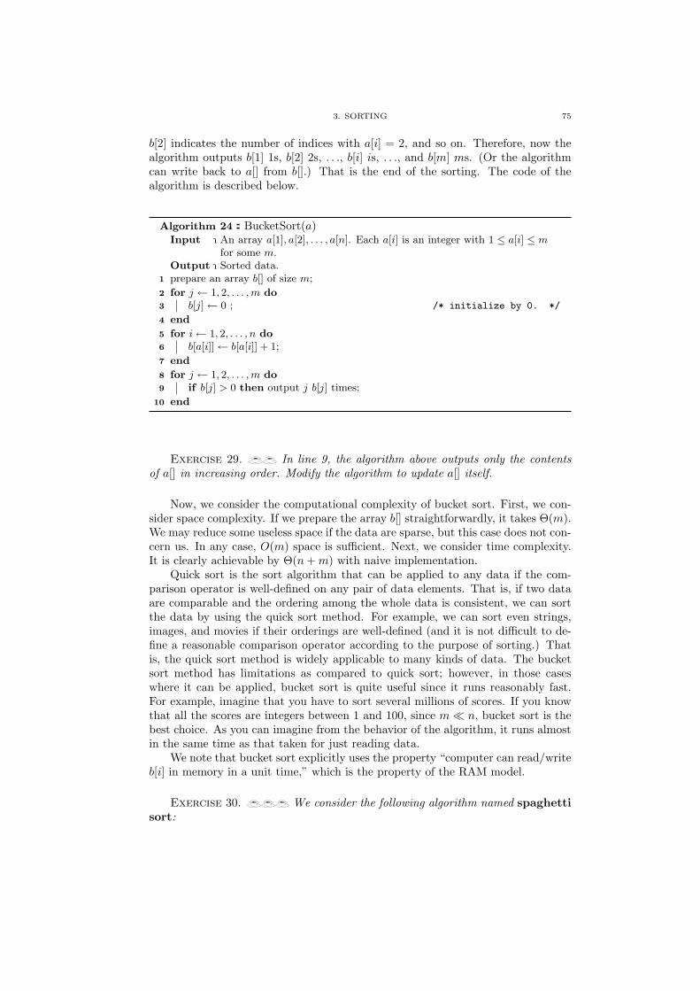
3. SORTING 75

b[2] indicates the number of indices with a[i] = 2, and so on. Therefore, now thealgorithm outputs b[1] 1s, b[2] 2s, . . ., b[i] is, . . ., and b[m] ms. (Or the algorithmcan write back to a[] from b[].) That is the end of the sorting. The code of thealgorithm is described below.

Algorithm 24：BucketSort(a)Input ：An array a[1], a[2], . . . , a[n]. Each a[i] is an integer with 1 ≤ a[i] ≤ m

for some m.Output ：Sorted data.

1 prepare an array b[] of size m;

2 for j ← 1, 2, . . . , m do3 b[j]← 0 ; /* initialize by 0. */

4 end

5 for i← 1, 2, . . . , n do6 b[a[i]]← b[a[i]] + 1;

7 end

8 for j ← 1, 2, . . . , m do9 if b[j] > 0 then output j b[j] times;

10 end

Exercise 29. In line 9, the algorithm above outputs only the contentsof a[] in increasing order. Modify the algorithm to update a[] itself.

Now, we consider the computational complexity of bucket sort. First, we con-sider space complexity. If we prepare the array b[] straightforwardly, it takes Θ(m).We may reduce some useless space if the data are sparse, but this case does not con-cern us. In any case, O(m) space is sufficient. Next, we consider time complexity.It is clearly achievable by Θ(n + m) with naive implementation.

Quick sort is the sort algorithm that can be applied to any data if the com-parison operator is well-defined on any pair of data elements. That is, if two dataare comparable and the ordering among the whole data is consistent, we can sortthe data by using the quick sort method. For example, we can sort even strings,images, and movies if their orderings are well-defined (and it is not difficult to de-fine a reasonable comparison operator according to the purpose of sorting.) Thatis, the quick sort method is widely applicable to many kinds of data. The bucketsort method has limitations as compared to quick sort; however, in those caseswhere it can be applied, bucket sort is quite useful since it runs reasonably fast.For example, imagine that you have to sort several millions of scores. If you knowthat all the scores are integers between 1 and 100, since m n, bucket sort is thebest choice. As you can imagine from the behavior of the algorithm, it runs almostin the same time as that taken for just reading data.

We note that bucket sort explicitly uses the property “computer can read/writeb[i] in memory in a unit time,” which is the property of the RAM model.

Exercise 30. We consider the following algorithm named spaghettisort:

76 3. ALGORITHMS FOR SEARCHING AND SORTING

Algorithm 25：SpaghettiSort(a)Input ：An Array a[1], a[2], . . . , a[n].Output ：Sorted array a[].

1 for i← 1, 2, . . . , n do2 cut dry spaghetti strands to length a[i];

3 end

4 bunch all the spaghetti strands in your left hand and stand them on your table;

5 for i← 1, 2, . . . , n do6 select the longest spaghetti strand in your right hand and put it on your table;

7 end

8 output the lengths of these spaghetti strands from one end to the other end;

Estimate the time complexity of this algorithm. Theoretically, it seems that thisalgorithm runs fast; however, you do would not like to use it. Why is this algorithmnot in practical use?

CHAPTER 4

Searching on graphs

bababababababababababababababab

The notion of a graph is a mathematical concept that was introduced torepresent a network of objects. The structure of a graph is very basic, andmany problems can be modeled using graphs. In this chapter, we learnbasic algorithms for searching a graph.

What you will learn: • Searching algorithms for graphs• Reachability• Shortest path problem• Search tree• Depth first search• Breadth first search• Dijkstra’s algorithm

77

78 4. SEARCHING ON GRAPHS

1. Problems on graphs

Have you ever seen a Web page that is public on the Internet on your personalcomputer or mobile phone? Of course, you have. The Web page has a usefulfunction that is called a hyperlink, and you can jump to another Web page to seeit just by a click. Suppose that when you open your usual Web page you happento think “I’d like to see that Web page I saw last week...” You remember that youreached that Web page by traversing a series of hyperlinks; however, you have nomemory of the route you traversed. This is nothing out of the ordinary.

Hyperlinks make up a typical graph structure. Each Web page corresponds to avertex in the graph, and each hyperlink joins two vertices. We do not know whetherthe entire graph is connected or disconnected. Searching problems for a graphare the problems that ask whether two vertices on a graph are reachable, that is,whether there is a route from one vertex to another on the graph. In this section,we consider the following three variants of the searching problem for a graph.

[Problem 1] Reachability problem:

Input: A graph G containing n vertices 1, 2, . . . , n. We assume that thestart vertex is 1 and the goal vertex is n.

Problem: Check whether there is any way that we can reach n from 1along the edges in G. The route is not important. The graph may bedisconnected. If we can reach n from 1 on G, output “Yes”; otherwise,output “No.”

[Problem 2] Shortest path problem:

Input: A graph G containing n vertices 1, 2, . . . , n. We assume that thestart vertex is 1 and the goal vertex is n.

Problem: We also assume that there is no cost for passing through eachedge; or we can also consider that each edge has a unit cost. Then,the problem is to find the length of the shortest path from 1 to n.Precisely, the length of a path is the number of edges along it. If n isnot reachable from 1, we define the length as ∞.

[Problem 3] Shortest path problem with minimum cost:

Input: A graph G containing n vertices 1, 2, . . . , n. We assume that thestart vertex is 1 and the goal vertex is n.

Problem: We also assume that each edge has its own positive cost.Then, the problem is to find the shortest path from 1 to n with mini-mum cost. The cost of a path is defined by the summation of the costof each of its edges. If n is not reachable from 1, we define the costas ∞.

It is easy to see that the above problems are all familiar in our daily life; theyappear in car navigation and route finder systems, and are solved every day. We

2. REACHABILITY: DEPTH-FIRST SEARCH ON GRAPHS 79

(1) (2)

6

1

5

74

2

32

1

5

74

6

3

Figure 1. Two examples of a graph.

learn how we can handle these problems and what algorithms and data structureswe can use to solve them.

2. Reachability: depth-first search on graphs

First, we consider Problem 1, which concerns the reachability in a given graph.For a given graph with n vertices 1, 2, . . . , n, we assume that the edge set is givenby the adjacency set. That is, the set of neighbors of the vertex i is represented byA[i, 1], A[i, 2], . . .. Hereafter, to simplify, we denote by di the number of elements inthe neighbor set of vertex i. (This number di is called the degree of vertex i.) Thatis, for example, the set of neighbors of vertex 2 is A[2, 1], A[2, 2], . . . , A[2, d2]. Thenumber di can be computed by checking whether A[i, j] = 0 for each j = 1, 2, . . . , di

in O(di) time. Thus, we can compute it every time we need to; alternatively, we cancompute it a priori and remember it in the array d[1], d[2], . . . , d[n]. The notationdi is used for convenience, and we do not consider the details of the implementationof this part.

Example 9. Consider the two graphs given in Figure 1. The adjacency setA1 of graph (1) on the left and the adjacency set A2 of graph (2) on the right aregiven as follows (the numbers are sorted in increasing order so that we can followthe algorithm easily).

A1 =

2 5 6 0 0 01 3 4 0 0 02 4 7 0 0 02 3 5 6 0 01 4 0 0 0 01 4 0 0 0 03 0 0 0 0 0

, A2 =

2 5 6 0 0 01 5 0 0 0 06 0 0 0 0 07 0 0 0 0 01 2 0 0 0 01 3 0 0 0 04 0 0 0 0 0

.

We use the following degree sequences for each graph: For graph (1), we haved[1] = 3, d[2] = 3, d[3] = 3, d[4] = 4, d[5] = 2, d[6] = 2, and d[7] = 1. Forgraph (2), we have d[1] = 3, d[2] = 2, d[3] = 1, d[4] = 1, d[5] = 2, d[6] = 2, andd[7] = 1. We assume that these arrays are already initialized before performing ouralgorithms.

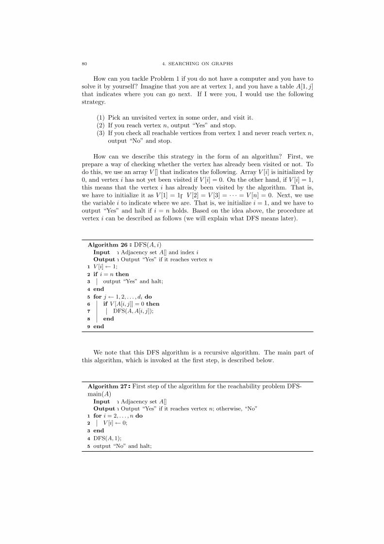
80 4. SEARCHING ON GRAPHS

How can you tackle Problem 1 if you do not have a computer and you have tosolve it by yourself? Imagine that you are at vertex 1, and you have a table A[1, j]that indicates where you can go next. If I were you, I would use the followingstrategy.

(1) Pick an unvisited vertex in some order, and visit it.(2) If you reach vertex n, output “Yes” and stop.(3) If you check all reachable vertices from vertex 1 and never reach vertex n,

output “No” and stop.

How can we describe this strategy in the form of an algorithm? First, weprepare a way of checking whether the vertex has already been visited or not. Todo this, we use an array V [] that indicates the following. Array V [i] is initialized by0, and vertex i has not yet been visited if V [i] = 0. On the other hand, if V [i] = 1,this means that the vertex i has already been visited by the algorithm. That is,we have to initialize it as V [1] = 1，V [2] = V [3] = · · · = V [n] = 0. Next, we usethe variable i to indicate where we are. That is, we initialize i = 1, and we have tooutput “Yes” and halt if i = n holds. Based on the idea above, the procedure atvertex i can be described as follows (we will explain what DFS means later).

Algorithm 26：DFS(A, i)Input ：Adjacency set A[] and index iOutput ：Output “Yes” if it reaches vertex n

1 V [i]← 1;

2 if i = n then3 output “Yes” and halt;

4 end

5 for j ← 1, 2, . . . , di do6 if V [A[i, j]] = 0 then7 DFS(A, A[i, j]);

8 end

9 end

We note that this DFS algorithm is a recursive algorithm. The main part ofthis algorithm, which is invoked at the first step, is described below.

Algorithm 27：First step of the algorithm for the reachability problem DFS-main(A)

Input ：Adjacency set A[]Output ：Output “Yes” if it reaches vertex n; otherwise, “No”

1 for i = 2, . . . , n do2 V [i]← 0;

3 end

4 DFS(A, 1);

5 output “No” and halt;

2. REACHABILITY: DEPTH-FIRST SEARCH ON GRAPHS 81

Structure of an algorithm Most algorithms can be divided into two parts containing respectively the“general process” and the “first step,” which contains initialization and invokesthe first process. This is conspicuous, particularly in recursive algorithms. Inthe algorithms up to this point in this book, the first step has been writtenin one line; we describe this in the main text. However, in general, we needsome pre-processing including the initialization of variables. Hereafter, thealgorithms named “∗-main” represent this first step, and the general processis located in the algorithm that has a name that does not include “main.”

This is the end of the algorithm’s description. Are you convinced that thisalgorithm works correctly? Somehow, you do not feel sure about the correctness,do you? Since this algorithm is written in recursive style, you may not be convincedwithout considering the behavior of the algorithm more carefully. First, to clarifythe reason why you do not feel sure, we consider the conditions when the algorithmhalts. The algorithm halts when one of two cases occurs:

• When i = n, that is, it reaches to the goal vertex. Then, it outputs “Yes”and halts.• In the DFS algorithm, the process completes the recursive calls in line 4

without outputting “Yes.” Then, the DFS-main outputs “No” in line 5and halts.

This would be all right in the first case. The algorithm certainly reaches the goalvertex n through the edges from the start vertex 1. The case that causes concern isthe second case. Is the answer “No” always correct? In other words, does it neverhappen that the algorithm outputs “No” even though a path exists from vertex 1to vertex n? This is the point. To understand this in depth, we first examine twotypical cases. The first case is where the algorithm outputs “Yes.”

Example 10. We perform the algorithm at vertex 1 in graph (1) in Figure 1.(We denote the array V by V1[] to distinguish the second example.) First, Algorithm27 performs the initialization in lines 1 to 3 and calls the procedure DFS(A1, 1). InDFS(A1, 1), DFS(A1, A1[1, 1] = 2) is again called in line 7. That is, it moves tothe neighbor vertex 2 from vertex 1. Then, Algorithm 26 is applied to vertex 2 andwe have the visited mark by setting V1[2] = 1. Since 2 6= n(= 7), the process movesto line 5. First, since V1[A1[2, 1]] = V1[1] = 1, it confirms that vertex 1 had alreadybeen visited; thus, it does not call DFS (in line 7) for this vertex 1. Next, sinceV1[A1[2, 2]] = V1[3] = 0, it finds that vertex 3 has not already been visited, callsDFS(A1, A1[2, 2]) in line 7, moves to vertex 3, and so on. Namely, it continues tocheck V1[], and does not visit it if it has already been visited; otherwise, it visits thisvertex. In this graph, the algorithm visits in the order

vertex 1→ vertex 2→ vertex 3→ vertex 4→ vertex 5→ vertex 6→ vertex 7

and outputs “Yes” when it visits the last vertex 7.

Next, we turn to the second example, that is, the “No” instance.

Example 11. We perform the algorithm at vertex 1 in graph (2) in Figure 1.(We denote the array V by V2[] this time.) As before, the algorithm visits vertices1, 2, and 5. When it visits vertex 5, it finds it has no more unvisited verticesfrom vertex 5. Then, the searching process in DFS(A2, A2[2, 2]) ends, and returns

82 4. SEARCHING ON GRAPHS

to vertex 1. This time, the DFS(A2, A2[1, 1]) is called in line 7 of Algorithm 26.In the next step, DFS(A2, A2[1, 2]) is not called because V2[A2[1, 2]] = V2[5] = 1.Then, DFS(A2, A2[1, 3]) is called since V2[A2[1, 3]] = V2[6] = 0, and the algorithmmoves to vertex 6. Then, it moves to vertex 3 from vertex 6, and finds that thereare no longer any unvisited vertices from vertex 3. Thus, this procedure call returnsto vertex 1; no more unvisited vertices exist, and hence the output is “No.”

You can understand this case in depth if you follow these “Yes” and “No”examples. Now we turn to the following case. The algorithm outputs “No” forsome reason, although it is possible to reach from vertex 1 to vertex n. Does thiscase never happen? The answer is never. It is not trivial, and so we here show theproof of this fact.

Theorem 10. The DFS algorithm for the reachability problem is certain tooutput “Yes” when it is possible to reach from vertex 1 to vertex n; otherwise, theoutput is “No.” In other words, this algorithm works correctly.

Proof. First, we check that this algorithm always halts in finite time regard-less of its output. It is clear that the algorithm always halts after two for state-ments. Therefore, we focus on the recursive call for DFS. There are two recursivecalls that the algorithm makes (line 7 in DFS and line 4 in DFS-main). In bothcases, DFS[A, i] is called for some i satisfying V [i] = 0. Then, immediately after-wards, V [i] ← 1 is performed at line 1 in DFS. Thus, once this recursive call hasbeen made for index i, the recursive call for DFS will be never performed for thisi again. On the other hand, the integer variable i takes its value with 1 ≤ i ≤ n.Therefore, the number of recursive calls in this algorithm is bounded above by n.Thus, this algorithm always halts with at most n recursive calls. The algorithm canhalt at line 3 in DFS and at line 5 in DFS-main, and hence, the algorithm outputseither “Yes” or “No” when it halts.

We first consider the case where the algorithm outputs “Yes.” In this case, thecorrectness of the algorithm is easy to see. From the construction of the algorithm,we can join the variables in the recursive calls of DFS and obtain the route fromvertex 1 to vertex n.

Next, we assume that the algorithm outputs “No” as the answer. Here, we havethe problem “Is this answer ‘No’ certainly correct?” We prove the correctness bycontradiction. We assume that there exists a graph G that includes a path joiningvertices 1 and n, and the DFS-main algorithm fails to find it and outputs “No.”Let P be the set of visited vertices during the journey that the algorithm traverseson G. Then, P contains vertex 1 by definition, and does not contain vertex n byassumption. On the other hand, since we assume that we can reach vertex n fromvertex 1, there is a path Q joining vertices 1 and n (if there are two or more, wecan select any one of them). Path Q starts from vertex 1 and ends at vertex n.We have common elements that belong to both P and Q; at least, vertex 1 is oneof the common elements. Among the common elements of P and Q, let i be theclosest vertex to n in Q. Since i belongs to P and P does not contain n, i is not n.Let k be the next vertex of i on Q (we note that k itself can be n). Then, by theassumption, P contains i, but does not contain k (Figure 2).

Now, P is the set of vertices visited by DFS. Thus, during the algorithm,DFS(A, i) should be called. In this procedure, for each neighbor A[i, j](j = 1, 2, . . . , di)of vertex i, the algorithm calls DFS(A,A[i, j]) if V [A[i, j]] = 0, that is, if vertex

2. REACHABILITY: DEPTH-FIRST SEARCH ON GRAPHS 83

1

k

n

iP

Q

Figure 2. Correctness of the algorithm for the reachability problem.

A[i, j] has not already been visited. Vertex k is one of the neighbors of i, and hence,A[i, j′] = k should hold for some j′, which means that DFS(A, k) should be calledfor this j′. This is a contradiction. Thus, such a vertex k does not exist.

Therefore, when vertex n is reachable from vertex 1, the DFS algorithm shouldfind a path from 1 to n and output “Yes.”

We here also state a theorem about the time complexity of the DFS algorithm.

Theorem 11. For a graph of n vertices with m edges, the DFS algorithm solvesthe reachability problem in O(n + m) time.

Proof. By careful observation of the DFS algorithm, it can be seen that thecrucial point is the estimation of the time complexity of the for loop. We canconsider this part as follows. Let us consider an edge i, j. For this edge, the algo-rithm performs the for loop at vertex i and another for loop at vertex j. This edgehad never been touched by another for loop. Therefore, the total time complexityconsumed by the for loops for each vertex can be bounded above the number ofedges up to constant. (A similar idea can be found in the proof of Theorem 3.)Therefore, summing the total running time O(n) for each vertex, the entire runningtime is O(n + m).

2.1. Search trees and depth-first search. Finally, we mention that whythe search method introduced in this section is called DFS. DFS is an abbreviationof “depth first search.” Then, what is searching in “depth first” style? We haveto learn about “search trees” to know what “depth first” means. We here focuson the ordering of visits. What property does the ordering of visited vertices bythe DFS algorithm have? Hereafter, we assume that the input graph is connected,since the DFS algorithm visits only the vertices in a connected component of theinput graph.

At the beginning of the search, we start from vertex 1. Therefore, each of theother vertices i with i 6= 1 is visited from another vertex if the graph is connected.

84 4. SEARCHING ON GRAPHS

1

5

74

3

2

6

Figure 3. Search tree in the graph in Figure 1(1) obtained byapplying the DFS algorithm.

Let j be the vertex from which the algorithm first visits vertex i. That is, the DFSalgorithm was staying at vertex j, and visits vertex i the first time through edgej, i. For each vertex from 2 to n, we can consider such an edge for visiting eachof them the first time. Vertex 1 is the only exception, having no such edge, becauseit is the vertex from which the DFS algorithm starts. Thus, the number of suchedges for visiting the first time is n − 1, and the graph is connected. Therefore,using Theorem 4, these edges form a tree in the input graph.

In this tree, vertex 1 is a special vertex. That is, the DFS algorithm startsfrom vertex 1 and visits all the vertices along the edges in this tree. This tree iscalled the search tree, and this special vertex 1 is called the root of the searchtree. It is useful that we assign the number to each vertex in the tree according tothe distance from the root. This number is called the depth of the vertex. Thedepth is defined by the following rules. First, the depth of the root is defined by 0.Then, the depth of the neighbors of the root is defined by 1. Similarly, the depthof a vertex is i if and only if there is a path of length i from the root to the vertexon the tree.

We now consider the ordering of the visits of the DFS algorithm on the searchtree from the viewpoint of the depth of the tree. The algorithm starts searchingfrom vertex 1 of depth 0 and selects one neighbor (vertex 2 in Figure 1(1)) of root 1.The next search target is the neighbor of this vertex 2 of depth 1. In Figure 1(1),vertex 3 is selected as the next vertex of vertex 2, and this vertex 3 has depth2, and so on. The search tree obtained by the DFS algorithm on the graph inFigure 1(1) is described in Figure 3. The search tree of the DFS algorithm is drawnin bold lines. Vertex 3 is visited as of depth 2, and vertices 4 and 7 are both visitedas of depth 3. On the other hand, we can consider another method of searching;for example, in Figure 3, after visiting vertex 2, the algorithm may visit vertices5 and 6. Namely, the algorithm first checks all the neighbors of the root beforemore distant vertices. However, the DFS algorithm, although there exist unvisitedvertices of smaller depth, gives precedence in its search to more distant or deepervertices. This is the reason why this algorithm is called “depth first search.”

Of course, the other method of searching, that is, searching all the vertices ofdepth 1 after checking the vertex of depth 0, before checking more distant vertices,gives us another searching option. While DFS prefers the depth direction for visiting

3. SHORTEST PATHS: BREADTH-FIRST SEARCH ON GRAPHS 85

the vertices in the tree, the second search method prefers the width or breadthdirection for searching. This method is called Breadth First Search; however,we will discuss the details of this algorithm in the next section.

Exercise 31. In the example in Figure 3, the DFS algorithm outputs“Yes” and halts when it reaches vertex 7. We now remove the line for output “Yes”from the algorithm and run it. Then, the algorithm, in any case, halts at output“No” after visiting all the vertices in the graph. Now, when we run this modifiedalgorithm on the graph given in Figure 1(1), what search tree do we obtain in thegraph?

3. Shortest paths: breadth-first search on graphs

Next, we turn to Problem 2, which is to find the shortest path. Since it istrivial when n = 1, hereafter we assume that n > 1. This time, we have to findnot only reachable vertices, but also the length of the shortest path from the startvertex 1 to the goal vertex n.

To consider how to solve this problem, imagine that we are inside vertex 1. Anatural idea is to explore the neighbor vertices of distance 1 from vertex 1 sincethey are reachable from the vertex 1 directly. If we find the goal vertex n in the setof vertices of distance 1 from vertex 1, we are done. Otherwise, we have to checkthe set of vertices of distance 2 from vertex 1 from each neighbor of vertex 1, and soon. In this manner, we can find the shortest path from vertex 1 to the goal vertexn. Therefore, briefly, we can solve the problem as follows.

(1) Visit each of the unvisited vertices in the order of their proximity to thestart vertex 1.

(2) If we arrive at the goal vertex n, output the distance to it and halt.(3) If we visit all reachable vertices, and still do not reach the goal vertex n,

output ∞ and halt.

In comparison to the reachability check, the key point is that we seek fromthe vertices closer to the start vertex 1. We now consider the search tree for thisalgorithm. The root is still vertex 1, which is not changed. The algorithm firstsweeps all the vertices that are neighbors of 1, and hence, are connected to theroot on the search tree; hence, they have depth 1 on the search tree. Similarly, thealgorithm next checks all the vertices that are neighbors of the vertices of distance1 from the root, or of depth 1 in the search tree, and hence, each is connected tosome vertex of distance 1. That is, the next vertices are of distance 2 from theroot, and also of depth 2 on the search tree. Therefore, each vertex of depth i onthe search tree is of distance i from the root on the original graph.

At a glance, one may think that we need a complicated data structure toimplement this algorithm; however, this is not the case. At this point, we have tothink carefully. Then, we can see that we can achieve this ordering of searchingeasily using the queue data structure. That is, the algorithm first initializes thequeue with the start vertex 1. After that, the algorithm picks up the top elementin the queue, checks whether the vertex i is n or not, and pushes all unvisitedneighbors of i into the queue if i is not n.

We consider the general situation of this queue. From the property of thequeue, we can observe the following lemma.

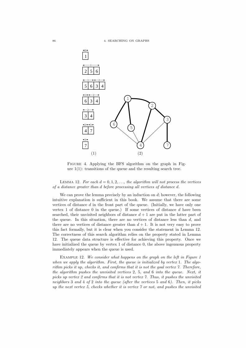
86 4. SEARCHING ON GRAPHS

2 5

3

1

6

5 6

36

43

4

7

0

1

1 2

1

2

2

3

4

4

2

7

3 6

1

5

74

2

3

(1) (2)

Figure 4. Applying the BFS algorithm on the graph in Fig-ure 1(1): transitions of the queue and the resulting search tree.

Lemma 12. For each d = 0, 1, 2, . . ., the algorithm will not process the verticesof a distance greater than d before processing all vertices of distance d.

We can prove the lemma precisely by an induction on d; however, the followingintuitive explanation is sufficient in this book. We assume that there are somevertices of distance d in the front part of the queue. (Initially, we have only onevertex 1 of distance 0 in the queue.) If some vertices of distance d have beensearched, their unvisited neighbors of distance d + 1 are put in the latter part ofthe queue. In this situation, there are no vertices of distance less than d, andthere are no vertices of distance greater than d + 1. It is not very easy to provethis fact formally, but it is clear when you consider the statement in Lemma 12.The correctness of this search algorithm relies on the property stated in Lemma12. The queue data structure is effective for achieving this property. Once wehave initialized the queue by vertex 1 of distance 0, the above ingenuous propertyimmediately appears when the queue is used.

Example 12. We consider what happens on the graph on the left in Figure 1when we apply the algorithm. First, the queue is initialized by vertex 1. The algo-rithm picks it up, checks it, and confirms that it is not the goal vertex 7. Therefore,the algorithm pushes the unvisited vertices 2, 5, and 6 into the queue. Next, itpicks up vertex 2 and confirms that it is not vertex 7. Thus, it pushes the unvisitedneighbors 3 and 4 of 2 into the queue (after the vertices 5 and 6). Then, it picksup the next vertex 5, checks whether it is vertex 7 or not, and pushes the unvisited

3. SHORTEST PATHS: BREADTH-FIRST SEARCH ON GRAPHS 87

neighbors to the end of the queue. The transitions of the queue and the depths ofthe vertices are depicted in Figure 4(1). The vertices are described by the numbersin the boxes, and the top of the queue is the left hand side. The numbers over theboxes are the depths of the vertex, that is, the distance from the root. The bold linesin Figure 4(2) show the resulting search tree.

We here mention one point to which we should pay attention. Let us considerthe viewpoint at vertex i. Once this vertex i is put into the queue, it will proceedin the queue, and in its turn, it will be checked as to whether it is the vertex n ornot. The point to which we have pay attention is that it is inefficient to put thisvertex i into the queue two or more times. (In fact, this can be quite inefficient insome cases. If you are a skillful programmer, this is a nice exercise to find such acase.) Let d be the distance from root 1 to vertex i. By Lemma 12, this inefficiencymay occur if vertex i has two neighbors, say j and k, of distance d− 1.

More precisely, an inefficient case may occur as follows. When two distinctvertices j and k of distance d− 1 are both adjacent to vertex i of distance d, bothvertices j and k may push vertex i into the queue. In Figure 4, once vertex 4 isput into queue, we have to avoid being put it again by vertices 3, 5 and 6 as theirneighbors. To avoid pushing vertex into the queue two or more times, let us prepareanother array C[]. For each vertex i, C[i] is initialized by 0. That is, if C[i] = 0,vertex i has not yet been pushed into the queue, and we define that C[i] = 1 meansthat vertex i has already been pushed into the queue. Once C[i] has been set at1, this value is retained throughout the algorithm. Each vertex ` should push itsneighbor i into the queue if and only if i is unvisited and C[i] = 0. When vertex i ispushed into the queue, do not forget to update C[i] = 1. When we check the DFSalgorithm carefully, we can see that we no longer need the array V [] to keep theinformation if “the vertex has already been visited.” Each vertex i in the queue,unless vertex n exists before it, will be visited at some time, and this informationis sufficient, even without V [].

At this time, the algorithm should output not only “Yes” or “No,” but also thelength of the shortest path to vertex n. Therefore, we use another array, say D[],to store the length of the shortest path to each vertex i. That is, D[i] = d meansthat we have the shortest path from vertex 1 to vertex i of length d. This value isset when the algorithm visits vertex i the first time, or when C[i] is set at 1 we donot need to initialize it.

We now consider what happens if the algorithm cannot reach vertex n. Withthe same argument as that of the DFS algorithm, all reachable vertices from vertex1 will be put into the queue. Therefore, if the queue becomes empty without vertexn being found, this implies that the desired answer is “∞.”

Based on the above discussion, the general case can be processed as follows.Note that the queue Q is one of arguments. (We will explain why this algorithm isnamed “BFS.”)

88 4. SEARCHING ON GRAPHS

Algorithm 28：BFS(A,Q)Input ：Adjacent set A[], queue QOutput ：The (shortest) distance from vertex 1 to vertex n

1 i← pop(Q);

2 if i = n then3 output D[i] and halt;

4 end

5 for j ← 1, 2, . . . , di do6 if C[A[i, j]] = 0 then7 push(Q, A[i, j]);

8 C[A[i, j]]← 1 ; /* Vertex A[i, j] is put into the queue */

9 D[A[i, j]]← D[i] + 1 ; /* We can reach j from i in 1 step */

10 end

11 end

The main part of this algorithm is as follows.

Algorithm 29：BFS-main(A)Input ：Adjacency set A[]Output ：Distance to vertex n if it is reachable; otherwise, “∞”

1 for i = 2, . . . , n do2 C[i]← 0;

3 end

4 C[1]← 1;

5 D[1]← 0;

6 push(Q, 1);

7 while sizeof(Q) 6= 0 do8 BFS(A, Q);

9 end

10 output ∞ and halt;

Exercise 32. In the BFS algorithm, two arrays C[] and D[] are used.When C[i] = 0, vertex i has not yet been placed into the queue, and C[i] = 1indicates that vertex i had been placed into the queue. When C[i] = 1, the value ofD[i] gives us the length of the shortest path from vertex 1 to vertex n. Somehow,this seems to be redundant. Consider how can you implement these two pieces ofinformation using one array. Is it an “improvement?”

Exercise 33. The above BFS algorithm outputs the distance of theshortest path to vertex n. However, it is natural to desire to output the shortestpath itself. Modify the above BFS algorithm to output one shortest path itself. It isnatural to output the path from vertex 1 to vertex n; however, it may be reasonableto output the path from vertex n to vertex 1, namely, to output the path in thereverse order.

Exercise 34. Prove the following two claims.(1) The BFS algorithm certainly outputs the length of the shortest path if

vertex n is reachable from vertex 1 on the graph.(2) The running time of the BFS algorithm is O(n+m), where n is the number

of vertices and m is the number of edges.

4. LOWEST COST PATHS: SEARCHING ON GRAPHS USING DIJKSTRA’S ALGORITHM 89

For the first claim, we can use an induction for the length of the shortest path. Inthis case, use Lemma 12 for the property of the queue. The proofs of Theorem 10and Theorem 11 are helpful.

We here mention the name of this algorithm, “BFS.” BFS stands for BreadthFirst Search. This algorithm first checks the root vertex 1 and then seeks allthe vertices of depth 1, that is, all the neighbors of the root. Then, it proceeds toseek all the vertices of depth 2. In this manner, in the search tree, this algorithmproceeds to the next depth after searching all the vertices of the same depth. Thiscan be regarded as a manner of searching that prefers to search in the “breadth”direction. Here, check again the search tree in Figure 4.

4. Lowest cost paths: searching on graphs using Dijkstra’s algorithm

We finally turn to the last problem, that is, finding the path of the lowest cost.This problem is more difficult than the previous two. Since each edge has its cost,we have to consider a detour that may give a lower total cost. The representative Edsger Wybe Dijk-

stra; 1930–2002:

Dijkstra’s algorithm

was conceived by

Edsger W. Dijkstra,

who was a computer

scientist well known

for this algorithm.

algorithm for this problem is called Dijkstra’s algorithm. In this section, welearn this algorithm.

Dijkstra’s algorithm is an algorithm for computing the minimum cost from thestart vertex 1 to the goal vertex n. We first prepare an array D[] for storing thiscost, which is initialized as D[i] = ∞ for each i. In the final step, D[i] stores theminimum cost to this vertex i from vertex 1. The cost for a path is defined by thesummation of the cost for each edge in this path. We also note that each cost of anedge is a positive value. We assume that each cost of an edge i, j is given by anelement of an array c(i, j). For convenience, we define it as c(i, j) = ∞ if there isno edge between these two vertices. Since every cost is positive, we have c(i, j) > 0for each i 6= j. We also define the cost as c(i, i) = 0 for all i. That is, we canmove from one vertex to itself with no cost. Moreover, since we are considering anundirected graph, we have c(i, j) = c(j, i) for any pair.

We first consider some trivial facts in order to consider the difficulty of theproblem. What are the trivial facts that we can observe? For moving from thestart vertex 1 to itself, the cost is trivial, namely, the cost of moving to vertex1 should be the minimum cost 0. Since all costs on edges are positive, we canmake no more improvements. That is, D[1] is definitely determined as 0. Whatnext? We consider the neighbors of vertex 1 to which we can move in one step. Wefocus on the costs on these edges. Let i be the neighbor of vertex 1 that has theminimum cost among all the edges incident to vertex 1. Then, this cost c(1, i) isthe minimum cost of moving to vertex i from vertex 1. The reason is simple. If wemove to another vertex to save the cost, then the cost is greater than or equal tothe cost c(1, i). (We remember the cost of each edge is positive, which means thatthe cost of this detour is not improved by passing more edges.) Therefore, amongthe neighbors of the vertex 1, for the vertex i that has the minimum cost c(1, ∗),we have D[i] = c(1, i).

Example 13. The above observation can be seen in Figure 5(1). We canconfirm D[i] = c(1, i) = 2 for vertex i, since it has the minimum cost among all theedges incident to vertex 1. As yet, we have no idea about the other vertices, sincesome cheaper detours may exist.

90 4. SEARCHING ON GRAPHS

1 2

4

58

j’

1i

2

(1)

1 2

4

58

j’

1i

2

(2)

j

Figure 5. Behavior of Dijkstra’s algorithm.

Now we have to consider the issue more carefully. The next vertices that canbe considered are the neighbors of the vertices 1 and i. Then, we have three sets ofvertices, that is, the vertices only adjacent to vertex 1, the vertices only adjacent tovertex i, and the vertices adjacent to both. Of course, we have to consider all thevertices in these three sets. Then, what do we have to compare this with? For thevertices j′ adjacent to only vertex 1, is it sufficient to consider the costs c(1, j′)?No, it is not. Possibly, there may be a cheaper detour starting from vertex i tovertex j′. In this case, of course, it takes additional cost c(1, i); however, it may beworthwhile. In Figure 5(1), we have an edge of cost 1 from vertex i to the upperright direction. This cheap edge may lead us to vertex j′ with a cost lower thanc(1, j′). We have a problem.

We consider the potential detour calmly. If there exists a cheaper detour thatpasses through vertex i, the cost of the neighbor of vertex i on the detour shouldbe low, and this cost is less than c(1, j′).

Investigating this point, we see that to “the nearest” neighbor vertex of bothvertices 1 and i, we have no cheaper detour since we do know the shortest routeto these vertices 1 and i. Therefore, we can compute the minimum cost to thisnearest neighbor. That is, we can conclude that the next vertex j to the ver-tices 1 and i for which we can compute the shortest path is the one that hasthe minimum cost to it from 1 and i. Precisely, this vertex j has the mini-mum value of minc(1, j), c(1, i) + c(i, j) for all the neighbors of vertices 1 andi. (Here, min returns the minimum value of the parameters, that is, the minimumvalue of c(1, j) and c(1, i) + c(i, j), in this case. Precisely, this vertex j satisfiesminc(1, j), c(1, i) + c(i, j) ≤ minc(1, j′), c(1, i) + c(i, j′) for any other vertex j′

in the neighbors of vertices 1 and i.) Thus, we have to find the vertex j with thiscondition and let D[j] = minc(1, j), c(1, i) + c(i, j).

Example 14. When the above discussion is applied to the case in Figure 5(1),we can determine vertex j as in Figure 5(2) and D[j] = c(1, i)+ c(i, j) = 2+1 = 3.We cannot yet fix D[] for the other vertices.

Thus far, we have a set S = 1, i, j of vertices for each of which we havecomputed the shortest route with the minimum cost from vertex 1. We can extendthe above idea to the other vertices. First, we summarize the procedure we followedto find the next vertex to be computed using extendable notations.

• First, for the start vertex 1, D[1] = c(1, 1) = 0 is determined. Let S = 1.

4. LOWEST COST PATHS: SEARCHING ON GRAPHS USING DIJKSTRA’S ALGORITHM 91

• Next, we find the minimum vertex i with respect to c(1, i), and D[i] =c(1, i) is determined. The set S is updated to S = 1, i.• Then, we find the minimum vertex j with respect to minD[1]+c(1, j), D[i]+

c(i, j), and D[j] = minD[1] + c(1, j), D[i] + c(i, j) is determined. Theset S is updated to S = 1, i, j.

In the last step, D[1] = 0 is added to the summation to clarify the meaning of theequation. We also replace c(1, i) with D[i] in this context. That is, in the generalstep, we have to find the “nearest” neighbor to the set of the vertices for whichthe minimum costs have already been computed. Then, we compute the minimumcost to the new nearest neighbor and add the vertex to the set S as the new onefor which the minimum cost is fixed.

Therefore, the procedure for the general case can be described as follows.• Find the closest neighbor vertex j to the set S of the vertices for which

the minimum cost of the path to them from the start vertex 1 has alreadybeen computed. More precisely, find the vertex j that has the minimumvalue of mini∈SD[i] + c(i, j) among all vertices j 6∈ S. The notation of

min:

The notation

mini∈SD[i] + c(i, j)means the minimum

value of D[i] + c(i, j)

for each vertex i in

the set S. It may be

difficult to see at the

first time; however, it

is concise and useful

if you become familiar

with it.

• For the vertex j with the minimum cost mini∈SD[i] + c(i, j), store it toD[j], and add j to the set S.

Note that we take the minimum value twice. That is, we essentially compute ashortest route to each vertex not in S, and find the nearest vertex among them.

We are now sure about the basic idea of the algorithm. However, when we tryto describe this idea in detail in the form of an algorithm that can be realized as acomputer program, we have to fill some gaps between the idea and the algorithm’sdescription. In particular, when we aim to implement this idea as an efficientalgorithm, there is still room for using devices.

We here introduce some useful tips for the implementation of Dijkstra’s algo-rithm. First, in addition to set S, we will use another set S of vertices that areadjacent to some vertices in S and are themselves not in S. In the above discussion,we considered the nearest neighbor vertex j to some vertex in S that consists ofvertices, the costs of which have been already computed. Vertex j should be in thisS. That is, when we seek vertex j with the condition, it is sufficient to search itonly in S, and we can ignore the other vertices in V \ (S ∪ S).

In the above discussion, we used an array D[] to store the cheapest cost D[i]from vertex 1 to vertex i, but we can make full use of this array not only for findingthe final cost. More specifically, for the vertices i, the array D[i] can store tentativedata as follows.

• When i is a vertex in S, as already defined, D[i] stores the cheapest costfrom vertex 1 to vertex i.• When i is a vertex not in (S ∪ S), we set D[i] =∞.• When i is a vertex in S, the array D[i] stores the cheapest cost from vertex

1 to vertex i through the vertices only in S ∪ i.

Example 15. We confirm the data structure in the graph in Figure 6. In thefigure, the set S = 1, 2, 4 is the set of vertices for which the minimum costs havebeen computed. Precisely, we have already D[1] = 0, D[2] = 2, and D[4] = 3, whichare the solutions for these vertices. Then, the set S is the set of neighbors of someelements in S, and hence, S = 5, 6, 7, 8, 9. For vertex 5, the tentative cheapestcost is D[5] = 4, which is easy to compute. For vertex 6, we go through only the

92 4. SEARCHING ON GRAPHS

3

5

1

9

2

4

58

1

2

8

1

6

4

3

4

2

2

7

3

SS

Figure 6. Progress of Dijkstra’s algorithm.

vertices in S ∪ 6 and we have D[6] = 8 so far. We can observe that this cost canbe reduced by passing vertex 7. That is, this D[6] will be improved in some futurestep. For vertex 7, the minimum cost is given by passing vertex 2 and hence wehave D[7] = 4. Similarly, we have D[8] = 6 and D[9] = 7 for vertices 8 and 9,respectively. For vertex 3, we have D[3] =∞ for this S (and S).

Using these data sets S, S and D, the required operations of the algorithm canbe summarized as follows.

Initialization: For a given graph, it lets S = 1, S = i | vertex i adjacent tothe vertex 1, and sets the array D as

D[1] = 0D[i] = c(1, i) for each i ∈ S

D[j] = ∞ for each j 6∈ S ∪ S.

General step: First, find the vertex j in S that takes the minimum value mini∈SD[i]+c(i, j) among mini∈SD[i] + c(i, j′) for all the vertices j′ in S. Set D[j] as thisminimum cost mini∈SD[i] + c(i, j), and add j into S. In this case, D[j] is fixedand will no longer be updated.

When the algorithm adds j into S, we have two things to do:• Add the neighbors of the vertex j not in S into S.• Update D[i′] for each vertex i′ satisfying D[i′] > D[j] + c(j, i′).

We give a supplementary explanation for the second process. Intuitively, by reasonof adding j into S, we obtain a cheaper route to vertices i′. We have two types ofsuch vertices; one has already been in S, and the other is added to S only in the firstprocess. (Note that no vertex in S is updated since there routes have been alreadyfixed.) For each vertex i′ just added into S in the first process, since D[i′] =∞, wecan update D[i′] = D[j] + c(j, i′) immediately. If vertex i′ has been in S already,we have to compare D[i′] with D[j] + c(j, i′), and update if D[i′] > D[j] + c(j, i′).

4.1. Implementations of Dijkstra’s algorithm. Now we understand Di-jkstra’s algorithm and the data structure that we need to perform the algorithm.In this section, we describe more details that allow us to implement it in a real

4. LOWEST COST PATHS: SEARCHING ON GRAPHS USING DIJKSTRA’S ALGORITHM 93

program. However, unfortunately, using only the data structures included in thisbook, we cannot implement a Dijkstra algorithm that runs “efficiently.” Therefore,we describe an implementation example using the data structures included in thisbook, and where we have a gap that can be improved. For advanced readers, itis a nice opportunity to investigate what data structure allows us to improve thisimplementation.

First, we consider the implementation of the sets S and S. When we considerthat there are some attributes belonging to each vertex, we can realize these setsby an array s[]. More specifically, we can define that vertex i is not in any set whens[i] = 0, s[i] = 1 means vertex i is in S, and s[i] = 2 means i is in S. That is, eachvertex i is initialized as s[i] = 0 and it changes to s[i] = 1 at some step, and finallywhen s[i] = 2, the value D[i] is fixed.

The crucial problem is how we can implement the following two processes cor-rectly.

• The process for finding vertex j in S that achieves the minimum value ofmini∈SD[i] + c(i, j).• After finding j above, the process involved when adding j into S.

We tentatively name the processes the function FindMinimum and the subrou-tine Update, respectively. Then, the main part of the Dijkstra algorithm can bedescribed as follows.

Algorithm 30：Dijkstra(A, c)Input ：Adjacent set A[] and cost function c[]Output ：Minimum cost D[i] to each vertex i from vertex 1

1 for i = 1, . . . , n do2 s[i]← 0;

3 end

4 D[1]← 0 ; /* Minimum cost to vertex 1 is fixed at 0. */

5 s[1]← 2 ; /* Vertex 1 belongs to set S */

6 for j = 1, . . . , d1 do7 s[A[1, j]]← 1 ; /* Put all neighbors of vertex 1 into S */

8 D[A[1, j]]← c(1, A[1, j]) ; /* Initialize by tentative cost */

9 end

10 while |S| < n do11 j ←FindMinimum(s, D, A);

12 Update(j, s, D, A);

13 end

14 output D[n];

This algorithm halts when all the vertices have been put into set S. Of course,it is sufficient that it halts when the goal vertex n is put into S. Here, we computethe minimum costs to all the vertices for the sake of simplicity. Hereafter, weconsider how we can implement the function FindMinimum and the subroutineUpdate.

Function FindMinimum: In this function, we have to find the vertex j fromS that gives the minimum value of mini∈SD[i] + c(i, j) for all vertices in S. Itis easier to see by changing the viewpoint to that of the edges to compute thisvalue. That is, if we can find an edge (i, j) such that i is in S, j is not in S,and D[i] + c(i, j) takes the minimum value among all edges (i′, j′) with i′ ∈ S and

94 4. SEARCHING ON GRAPHS

j′ 6∈ S, this j not in S is the desired vertex. Therefore, the following algorithmcomputes this function simply. The variable min keeps the current minimum valueof D[i] + c(i, j), and the variable jm keeps the current vertex that gives the valueof min. We have to initialize min by ∞. The variable jm does not need to beinitialized since it will be updated when min is updated.

Algorithm 31：Function FindMinimum(s, D, A)Input ：s[], D[], A[]Output ：Vertex j that gives mini∈SD[i] + c(i, j)

1 min←∞;

2 for i = 1, . . . , n do3 if s[i] = 2 then /* vertex i is in S */

4 for j = A[i, 1], . . . , A[i, di] do5 if s[j] = 1 then /* vertex j is in S */

6 if min > D[i] + c(i, j) then7 min← D[i] + c(i, j);

8 jm ← j;

9 end

10 end

11 end

12 end

13 end

14 return jm;

The running time of the algorithm does not concern us. This algorithm maytouch every vertex and every edge in constant time, and therefore, the running timeof one call of FindMinimum is O(n + m). In this implementation, there are twopoints involving redundancy that can be improved:

• In the algorithm, it checks every edge; however, it needs to check onlyeach edge of which one endpoint is in S and the other is in S.• The function FindMinimum is called repeatedly, and at each call, it com-

putes D[i]+ c(i, j) for all edges, finds the edge i, j having the minimumvalue, and discards all the values of D[i] + c(i, j). When the algorithmfinds the edge i, j, it updates the information around the vertex j andits neighbors by calling Update. This update propagates only locallyaround vertex j. That is, when the function FindMinimum is called thenext time, for almost all edges, D[i] + c(i, j) is not changed from the lasttime.

Therefore, one reasonable idea is to maintain only the edges joining the sets S andS in a linked list structure. Then, in each step, if we maintain the neighbors of themodified edges with the least cost, we can reduce the running time for the functionFindMinimum. More precise details of this implementation and the improvementof time complexity are beyond the scope of this book and so we stop here.

Subroutine Update: In this subroutine, we have to move vertex j from set S toset S. This process itself is easy; we just update s[j] = 1 to s[j] = 2. However, wehave to handle the associated vertices k adjacent to vertex j. For them, we haveto consider three cases:

• The vertex k is already in S: In this case, we already have the least costin D[k], and we have nothing to do.

4. LOWEST COST PATHS: SEARCHING ON GRAPHS USING DIJKSTRA’S ALGORITHM 95

• The vertex k is in S: In this case, since the edge j, k may give a shortcut to the vertex k, we have to update D[k] to D[j]+c(j, k) if D[j]+c(j, k)is less than the current D[k].• The vertex k is not in both S and S: In this case, the edge j, k gives us

a tentative shortest route to the vertex k, and hence, we can set the newcost D[j] + c(j, k) to D[k].

At a glance, these three cases are complicated. However, when we consider the twopoints

• All D[k]s are initialized by ∞ at first, and• D[k] gives the least cost if vertex k is already in S,

the following one process correctly deals with the above three cases simultaneously.

• If D[k] > D[j] + c(j, k), let D[k] = D[j] + c(j, k).

Therefore, the implementation of the subroutine Update can be given in thefollowing simple form.

Algorithm 32：Subroutine Update(j, s, D, A)Input ：j, s[], D[], A[]Output ：Move vertex j into set S

1 s[j]← 2;

2 for i = 1, . . . , dj do3 if s[A[j, i]] = 0 then4 s[A[j, i]] = 1 ; /* add k = A[j, i] to S */

5 end

6 if D[A[j, i]] > D[j] + c(j, A[j, i]) then7 D[A[j, i]]← D[j] + c(j, A[j, i]);

8 end

9 end

In this implementation, the subroutine Update runs in O(d(j)) time, whered(j) is the degree, or the number, of neighbors, of the vertex j. It is difficult toessentially improve this part. However, we do not need to process the neighborsalready in S; it can run a bit faster if we can skip them.

4.2. Analysis of Dijkstra’s algorithm. As described previously, the imple-mentation in this book is not so efficient that there is no room for improvement.However, it is a nice exercise for readers to evaluate the time complexity of thesimple implementation above.

In the main part of Dijkstra’s algorithm, the initialization takes O(n) time,and the while statement is also repeated in O(n) time. In this while, the functionFindMinimum performs in O(n + m) time, and the subroutine Update runs inO(d(j)) time. Therefore, n repeats of the function FindMinimum dominate therunning time, and hence, the total running time is estimated as O(n(n + m)) time.In a general graph, the number of edges can be bounded above by n(n − 1)/2, orO(n2). Thus, Dijkstra’s algorithm in this implementation runs in O(n3) time. Ifwe adopt a more sophisticated data structure with fine analysis, it is known thatDijkstra’s algorithm can be improved to O(n2) time.

96 4. SEARCHING ON GRAPHS

Current route finding algorithm is... On an edge-weighted graph, the shortest path problem with minimum cost issimple but deep. Although the basic idea of Dijkstra’s algorithm is not verydifficult, we now feel keenly that we need some nontrivial tricks that can beimplemented so that it runs efficiently. Some readers may feel that such agraph search problem is certainly interesting, but is a so-called toy problem,that is, it is artificial and has few applications. However, this is not the case.You are daily served by such algorithms for solving graph search problems. Forexample, consider your car navigation system, or your cellular phone. In sucha device, there exists a program for solving graph search problems. When yougo to an unfamiliar place by car or by public transportation, by any route, youhave to solve the graph search problem. This is, essentially, the shortest pathproblem with minimum cost. Some decades ago, in such a case, you would havetackled this problem by yourself using maps and time tables. Moreover, thiswould not necessarily have given you the best solution. However, nowadays,anybody can solve this shortest path problem easily by using an electric device.We owe the development of efficient algorithms for this problem a great debtof gratitude.Since it is in demand from the viewpoint of applications, research on graphsearch algorithms is still active. There are international competitions for solv-ing these problems in the shortest time. The up-to-date algorithms can solvethe graph search problems even if a graph has tens of thousands of vertices.For example, for the map of United States, they can find a shortest path be-tween any two towns in some milliseconds, which is amazing. As comparedto the simple(!) Dijkstra’s algorithm, these algorithms use very many detailedtechniques to make them faster. For example, on some specific map, they useknowledge such as “It is not likely that the shortest path passes a point thatis farthest from the start point,” “Main roads (such as highways) are likely tobe used,” “Beforehand, compute the shortest paths among some major land-marks,” and so on.

Index

記号if-statement ·············································15

A

address ·················································4, 11

adjacent ···················································32

algorithm ···················································3analog computer ········································2array ························································12

ASCII·······················································12

assembly language ·····································6assertion···················································66

B

backtracking ············································97

binary search ···········································54

binary tree ·············································117

bit ······························································2block search ·············································52

Breadth First Search ·························85, 89

bubble sort···············································59bucket sort ···············································74

C

caching ·····················································17

collision ····················································57

compiler ·····················································7computational complexity························10

computational geometry ····························8connected ·················································33

control statements ···································13

convex hull ·············································139

coupon collector’s problem ····················120

CPU (Central Processing Unit) ·················4

D

degree ·········································· 26, 33, 79

depth························································84

Digital computer········································2Dijkstra’s algorithm ·································89

directed graph··········································32

divide and conquer ······················ 48, 60, 64

DNA computer ··········································8Dynamic programming ····························48

E

edge··························································32Euler’s constant ·······································29expected value ·········································72exponential explosion·······························27

F

FIFO(First In, First Out)························17FILO(First In, Last Out) ························17finite control ······································2, 4, 5

flag ···························································62Folding paper in half ·····························131function····················································15

G

global variables ········································43golden ratio··············································48graph ·······················································32

H

harmonic number ·····································29harmonic series ········································29hash ·························································56hash function ···········································56hash value ················································57head ···························································2high-level programming language ··············7Horner method ······································131hyperlink··················································78

I

in-degree ··················································33index ························································12intractable················································26

K

key ···························································57

L

l’Hospital’s rule································ 28, 129

leaf ···························································34LIFO(Last In, First Out)·························17linearity of expectation ····························72local variables ··········································43

151

152 INDEX

M

machine language···································6, 7

Machine model···········································2RAM model············································2Turing machine model····························2Turing machine model····························2

memory ······················································4merge sort ················································60Mersenne twister····································114

motor ·························································2

N

Natural number ·········································2numerical computation ······························8

O

OCW (OpenCourseWare) ······················124

OEIS (On-Line Encyclopedia of IntegerSequences) ····································· 146

optimization·············································17

out-degree ················································33overflow····················································19

P

parameters ···············································13

parity ·····················································106

pigeon hole principle ································98

pivot·························································64

program counter ········································5pruning ··················································110

pseudo random numbers ························114

Q

quantum computer ····································8queuing ····················································17quick sort ···········································11, 64

R

RAM (Random Access Machine) model ····3RAM model ···············································3random number ·····································114

randomization ··········································11

randomized algorithms ··························113

registers ·····················································5root ··························································84

S

scale free ··················································36

search tree················································84Searching problems ··································78seed ························································114

sentinel·····················································51simple graph ············································32space complexity··································9, 10

spaghetti sort ···········································75stable ·······················································58stack ························································18Stirling’s formula ·····································74subroutine ················································15

substitution··············································13

T

tape····························································2the eight queen puzzle ·····························98theory of computation ·······························3time complexity ···································9, 10

tree ··························································33trees ·························································33trivial lower bound ··································24Turing machine ··········································2Turing machine model ·······························2

U

undirected graph······································32Unicode····················································12uniformly at random······························114

Vvariable ················································6, 12vertex·······················································32

Wword···························································4