Firefly-Inspired Sensor Network Synchronicitywith Realistic Radio Effects

Geoffrey Werner-Allen, Geetika Tewari, Ankit Patel, Matt Welsh, Radhika NagpalDivision of Engineering and Applied Sciences

Harvard University{werner,gtewari,abpatel,mdw,rad}@eecs.harvard.edu

ABSTRACTSynchronicity is a useful abstraction in many sensor net-work applications. Communication scheduling, coordinatedduty cycling, and time synchronization can make use of asynchronicity primitive that achieves a tight alignment ofindividual nodes’ firing phases. In this paper we presentthe Reachback Firefly Algorithm (RFA), a decentralized syn-chronicity algorithm implemented on TinyOS-based motes.Our algorithm is based on a mathematical model that de-scribes how fireflies and neurons spontaneously synchronize.Previous work has assumed idealized nodes and not consid-ered realistic effects of sensor network communication, suchas message delays and loss. Our algorithm accounts for theseeffects by allowing nodes to use delayed information fromthe past to adjust the future firing phase. We present anevaluation of RFA that proceeds on three fronts. First, weprove the convergence of our algorithm in simple cases andpredict the effect of parameter choices. Second, we leveragethe TinyOS simulator to investigate the effects of varyingparameter choice and network topology. Finally, we presentresults obtained on an indoor sensor network testbed demon-strating that our algorithm can synchronize sensor networkdevices to within 100 µsec on a real multi-hop topology withlinks of varying quality.

Categories and Subject DescriptorsC.2 [Computer-Communication Networks]: NetworkArchitecture and Design, Distributed Systems

General TermsAlgorithms, Design, Experimentation, Theory

KeywordsSynchronization, Wireless Sensor Networks, Biologically In-spired Algorithms, Pulse-Coupled Oscillators

Permission to make digital or hard copies of all or part of this work forpersonal or classroom use is granted without fee provided that copies arenot made or distributed for profit or commercial advantage and that copiesbear this notice and the full citation on the first page. To copy otherwise, torepublish, to post on servers or to redistribute to lists, requires prior specificpermission and/or a fee.SenSys’05,November 2–4, 2005, San Diego, California, USA.Copyright 2005 ACM 1-59593-054-X/05/0011 ...$5.00.

1. INTRODUCTIONComputer scientists have often looked to nature for inspi-

ration. Researchers studying distributed systems have longenvied, and attempted to duplicate, the fault-tolerance anddecentralized control achieved in natural systems. Those ofus studying sensor networks also have every reason to beenvious. Designing software coordinating the output of acollection of limited devices frequently feels as frustratingas orchestrating the activity of a colony of stubborn ants, orguiding a school of uncooperative fish. And yet ant coloniescomplete difficult tasks, schools of fish navigate the sea, andswarms of fireflies stretching for miles can pulse in perfectunison, all without centralized control or perfect individ-uals. The spontaneous emergence of synchronicity — forexample, fireflies flashing in unison or cardiac cells firing insynchrony — has long attracted the attention of biologists,mathematicians and computer scientists.

Synchronicity is a powerful primitive for sensor networks.We define synchronicity as the ability to organize simulta-neous collective action across a sensor network. Synchronic-ity is not the same as time synchronization: the latter im-plies that nodes share a common notion of time that canbe mapped back onto a real-world clock, while the formeronly requires that nodes agree on a firing period and phase.The two primitives are complementary: nodes with accessto a common time base can schedule collective action inthe future, and conversely, nodes that can arrange collectiveaction can establish a meaningful network-wide time base.However, the two primitives are also independently useful.For example, nodes within a sensor network may want tocompare the times at which they detected some event. Thistask requires a notion of global time, however it does notrequire real-time coordination of actions.

Similarly, synchronicity by itself can be extremely usefulas a sensor network coordination primitive. A commonly-used mechanism for limiting energy use is to carefully sched-ule node duty cycles so that all nodes in a network (or a por-tion of the network) will wake up at the same time, sampletheir sensors, and relay data along a routing path to the basestation. Coordinated communication scheduling has beenused both at the MAC level [18] and in multi-hop routingprotocols [12] to save energy. Synchronicity can also be usedto coordinate sampling across multiple nodes in a network,which is especially important in applications with high datarates. Previous work on seismic analysis of structures [1],shooter localization [13], and volcanic monitoring [15] coulduse such a primitive and avoid the overhead of maintainingconsensus on global time until absolutely necessary.

In this paper, we present a biologically-inspired distributedsynchronicity algorithm implemented on TinyOS motes. Thisalgorithm is based on a mathematical model originally pro-posed by Mirollo and Strogatz to explain how neurons andfireflies spontaneously synchronize [10]. This seminal workproved that a very simple reactive node behavior would al-ways converge to produce global synchronicity, irrespectiveof the number of nodes and starting times. Recently Lu-carelli and Wang [8] demonstrated that this result also holdsfor multi-hop topologies, an important contribution towardsmaking the model feasible for sensor networks.

The firefly-inspired synchronization described by Mirolloand Strogatz has several salient features that make it attrac-tive for sensor networks. Nodes execute very simple com-putations and interactions, and maintain no internal stateregarding neighbors or network topology. As a result, thealgorithm robustly adapts to changes such as the loss andaddition of nodes and links [8]. The synchronicity provablyemerges in a completely decentralized manner, without anyexplicit leaders and irrespective of the starting state.

However, implementing this approach on wireless sensornetworks still presents significant obstacles. In particular,the previous theoretical work assumes instantaneous com-munication between nodes. In real sensor networks, radiocontention and processing latency lead to significant andunpredictable communication latencies. Earlier work alsoassumes non-lossy radio links, identical oscillator frequen-cies, and arbitrary-precision floating-point arithmetic whichare unrealistic in current sensor networks.

We present the reachback firefly algorithm (RFA) that ac-counts for communication latencies, by modifying the origi-nal firefly model to allow nodes to use information from thepast to adjust the future firing phase. We evaluate our al-gorithm in three ways: theory, simulation and implementa-tion. We present theoretical results to prove the convergenceof our algorithm in simple cases and predict the impact ofparameter choice. Next we leverage TOSSIM, the TinyOSsimulator, to explore the behavior of the algorithm over arange of parameter values, varying numbers of nodes, anddifferent communication topologies. These simulation re-sults validate the theoretical predictions. Finally, we presentresults from experiments on a real sensor network testbed.These results demonstrate that our algorithm is robust inthe face of real radio effects and node limitations. Our re-sults show that such a decentralized approach can providesynchronicity to within 100 µsec on a complex multiple-hopnetwork with asymmetric and lossy links. To the best of ourknowledge, this work represents the first implementation offirefly-inspired synchronicity on the MicaZ mote hardware,and demonstrates the ability of the model to achieve syn-chronicity given real radio and hardware limitations.

Our paper is organized as follows. Section 2 presents re-lated work. In Section 3 we present RFA in the context ofthe Mirollo and Strogatz model and describe current hard-ware and radio limitations. Sections 4-7 present our metricsand theoretical, simulation and experimental results. Weconclude with future work.

2. BACKGROUND AND MOTIVATIONTime synchronization has received a great deal of atten-

tion in the sensor network community. The problem of es-tablishing a consistent global timebase across a large net-work, despite message loss and delays, node failures, and lo-

cal clock skew, has proven to be very difficult. As describedin the introduction, our goal is not time synchronization,but rather synchronicity: the ability for all nodes in thenetwork to agree on a common period and phase for firingpulses. Synchronicity can be used to implement time syn-chronization, although this requires mapping the local firingcycle to a global clock, which we leave for future work.

2.1 Time SynchronizationA number of protocols have been proposed that allow

wireless sensor nodes to agree on a common global timebase.Here we briefly describe some of the protocols. In ReceiverBased Synchronization (RBS) [2] a reference node broad-casts a message and multiple receivers within radio rangecan then agree on a common time base by exchanging thelocal clock times at which they received the message. Thisprotocol avoids the uncertainty of transmission delays byusing a single radio message to simultaneously synchronizemultiple receiver nodes, however it does not apply in multi-hop networks. The TPSN [3] protocol works on multi-hopnetworks by constructing a spanning tree and then usinghop-by-hop synchronization along the edges to synchronizeall nodes to the root. They also introduce MAC level times-tamping to estimate transmission delay. The FTSP proto-col [9], simplifies the process of multi-hop synchronizationby using periodic floods from an elected root, rather thanmaintaining a spanning tree. In the case of root failure,the system elects a new root node. FTSP also refines thetimestamping process to within microsecond accuracy andprovides a method for estimating clock drift which reducesthe need to synchronize frequently.

Direct comparison of these protocols in terms of synchro-nization error is difficult, due to the differences in hard-ware and evaluation methodology. FTSP reports a per-hopsynchronization error of about 1 µsec, although the maxi-mum pairwise error is over 65 µsec in their testbed. Themean single-hop synchronization error reported for TPSN is16.9 µsec, compared to 29.1 µsec for RBS [3]. The dynamicsof these protocols in terms of robustness to topology changesand node population have not been widely studied.

2.2 Biologically-Inspired SynchronicitySynchronicity has been observed in large biological swarms

where individuals follow simple coordination strategies. Thecanonical example is the synchrony of fireflies observed incertain parts of southeast Asia [10]. The behavior of thesesystems can be modeled as a network of pulse-coupled os-cillators where each node is an oscillator that periodicallyemits a self-generated pulse. Upon observing other oscilla-tors’ pulses, a node adjusts the phase of its own oscillatorslightly. This simple feedback process results in the nodestightly aligning their phases and achieving synchronicity.

Peskin first introduced this model in the context of cardiacpacemaker cells[11]. Mirollo and Strogatz [10] provide oneof the earliest complete analytical studies of pulse-coupledoscillator systems. They proved that a fully-connected (all-to-all) network of N identical pulse-coupled oscillators wouldsynchronize, for any N and any initial starting times. Re-cent work by Lucarelli and Wang [8] relaxes the all-to-allcommunication assumption. Drawing from recent results inmulti-agent control, they derive a stability result based onnearest neighbor coupling and show convergence in simu-lation for static and time varying topologies. Their work

demonstrates that the same simple feedback process works,even when nodes only observe nearest neighbors and thoseneighbors may change over time.

Several groups have proposed using pulse-coupled syn-chronicity to solve various network problems. Hong andScaglione [6, 5] introduce an adaptive distributed time syn-chronization method for fully-connected Ultra Wideband(UWB) networks. They use this as a basis for change de-tection consensus. Wakamiya and Murata [14] propose ascheme for data fusion in sensor networks where informationcollected by sensors is periodically propagated without anycentralized control from the edge of a sensor network to abase station, using pulse-coupled synchronicity. Wokoma etal. [17] propose a weakly coupled adaptive gossip protocol foractive networks. Each of these applications clearly demon-strates the utility of synchronicity as a primitive. Howevermuch of the prior work is evaluated only in simulation anddoes not consider real communication delay or loss.

Wireless radios exhibit non-negligible and unpredictabledelays due to channel coding, bit serialization, and (mostimportantly) backoff at the MAC layer [3, 9]. In traditionalCSMA MAC schemes, a transmitter will delay a randominterval before initiating transmission once the channel isclear. Additional random (typically exponential) backoffsare incurred during channel contention. On the receivingend, jitter caused by interrupt overhead and packet dese-rialization leads to additional unpredictable delays. Radiocontention deeply impacts the firefly model. Multiple nodesattempting to fire simultaneously will be unable to do so bythe very nature of the CSMA algorithm. As nodes achievetighter synchronicity, contention will become increasinglyworse as many nodes attempt to transmit simultaneously.The goal of this paper is to address the limitations of currentcommunication assumptions and realize a real implementa-tion of firefly-inspired synchronicity in sensor networks.

3. FIREFLY-INSPIRED SYNCHRONICITYIn this section, we first describe the Mirollo and Strogatz

model and discuss how the theoretical model differs frompractice. Then we present our modified algorithm, whichtakes these differences into account.

3.1 Mirollo and Strogatz ModelIn the Mirollo and Strogatz (M&S) model, a node acts as

an oscillator with a fixed time period T . Each node has aninternal time or phase t, which starts at zero and incrementsat a constant rate until t = T . At this point the node “fires”(in the case of firefly, flashes) and resets t = 0. Nodes maystart at different times, therefore their internal time (phase)t is not synchronized.

In the absence of any input from neighbors, a node Bsimply fires whenever t = T . If B observes a neighbor firing,then B reacts by adjusting its phase forward, thus shorteningits own time to fire (Figure 1(a,b)).

The amount of adjustment is determined by the functionf(t), which is called the firing function, and the parameterε, which is a small constant < 1. Suppose node B observes aneighbor fire at t = t′. In response, node B instantaneouslyjumps to a new internal time t = t′′, where

t′′ = f−1(f(t′) + ε) (1)

However if t′′ > T , then t = T and the node immediately

fires and resets t = 0. In a biological sense, f(t) can bethought of as the charge of a capacitor within the neuron orfirefly, which receives a boost of ε whenever a firing event isobserved. Algorithmically, the effect is that a node instan-taneously increments its phase by ∆(t′) = (t′′ − t′), when itobserves a firing event at t = t′.

The seminal result by Mirollo and Strogatz is that if thefunction f is smooth, monotonically increasing, and concavedown, then a set of n nodes will always converge to the samephase (i.e achieve synchronicity), for any n and any initialstarting times [10]. The simple requirements on f ensurethat a node reacts more strongly to events that occur laterin its time period. One of the limitations of their proof wasthat it only held for the case where all n nodes could observeeach others’ firing (all-to-all topology). Recently Lucarelliand Wang [8] relaxed this condition and proved that thissimple node behavior also results in synchrony in multi-hoptopologies, a prerequisite for use in sensor networks.

3.2 From Theory to PracticeThe M&S model has several salient features. The node

algorithm and the communication are very simple. A nodeonly needs to observe firing events from neighbors — there isno strength associated with the event or even a need to knowwhich neighbor reported the event. Individual nodes have nostate other than their internal time. Synchronicity provablyemerges without any explicit leaders and irrespective of thestarting state.

Because of these reasons, the model is particularly at-tractive as an algorithm for sensor networks. However, thetheoretical results in [10, 8] make several assumptions whichare problematic for wireless sensor networks. These include:

1. When a node fires, its neighbors instantaneously ob-serve that event.

2. Nodes can instantaneously react by firing.

3. Nodes can compute f and f−1 perfectly using contin-uous mathematics and can compute instantaneously.

4. All nodes have the same time period T .

5. Nodes observe all events from their neighbors (no loss).

In a wireless setting, a firing event can be implemented asa node sending a broadcast message to its neighbors indicat-ing that it fired. However, as mentioned before, nodes expe-rience an unpredictable delay prior to transmission, basedon channel contention. Thus, when a node A sends out afiring event message at time t, its neighbor B will not re-ceive the message until time t + δ where the delay δ is notknown in advance. This violates assumptions 1 and 2. NodeB does not know when the actual firing event occurred andnode B can not react instantaneously to node A’s behavior.In addition, the best case for the theoretical model — i.e.all nodes fire simultaneously — constitutes a worst case sce-nario for channel contention because it creates the potentialfor many collisions, resulting in large message delays.

The other assumptions also pose potential problems, thoughnot quite as problematic as message delays. Computationaccuracy is limited due to the absence of efficient floatingpoint arithmetic. Sensor nodes exhibit slightly different os-cillator frequencies. Links between nodes exhibit varyingquality and thus varying levels of message loss. At the same

Time in absolute units

No

de

’sin

tern

altim

e(t)

100

0 100 2000

No

de

’sin

tern

altim

e(t)

0 30 10040 70 175

100

0

45

30

0 30 10040 70 175

100

0

No

de

’sin

tern

altim

e(t)

(a)

(c)

(b)

t = 25

95

35

55

85

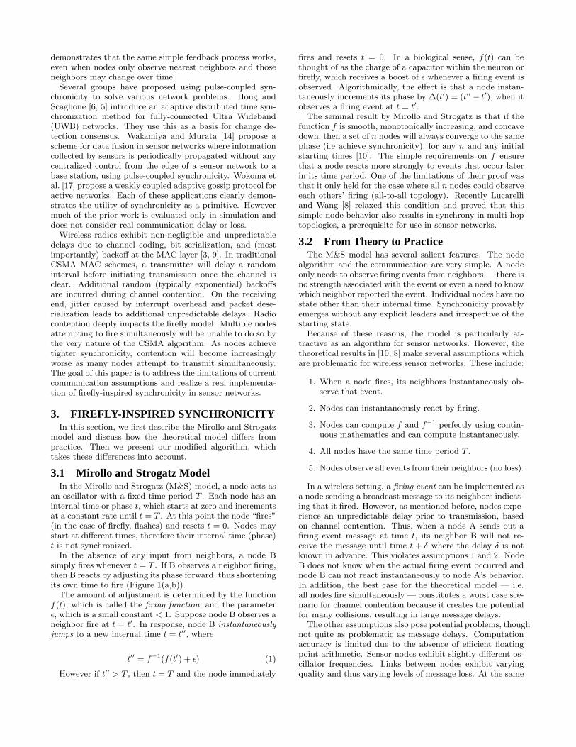
Figure 1: The firefly-inspired node algorithm. (a)A node fires whenever its internal time t is equal tothe default time period T (=100). (b) In the M&Smodel, a node responds to neighbors firing (arrows)by instantaneously incrementing t. (c) In RFA, anode records the firing events and then responds allat once at the beginning of the next cycle.

time, real biological systems are known to have such varia-tions. Therefore not all of the theoretical assumptions maybe important in practice.

3.3 The Reachback Firefly Algorithm (RFA)In this paper we focus mainly on the issues related to wire-

less communication. We tackle the three problems relatedto wireless communication in the following way: (1) We uselow level timestamping to estimate the amount of time amessage was delayed before being broadcast; (2) we modifythe node algorithm and introduce the notion of “reachback”in which a node reacts to messages from the previous timeperiod rather than the current time period, and (3) we pre-emptively stagger messages to avoid worst case wireless con-tention. Lastly, we use a simple, approximate firing functionthat can be computed quickly.

Timestamping Messages. In order to estimate thedelay between when a node “fires” and when the actualmessage is transmitted, we use MAC-layer timestamping torecord the MAC delay experienced by a message prior totransmission. The MAC delay can be measured by an eventtriggered by the TinyOS radio stack when the message isabout to be transmitted, and is recorded in the header ofthe outgoing message. When a node receives a firing mes-sage, it uses this information to determine the correct firingtime of the transmitting node by subtracting the MAC delay

from the reception time of the message. This is very similarto the approach used in time synchronization protocols suchas FTSP [9] to estimate message transmission delays.

The Reachback Response. The timestamping allows anode B to correctly identify when a neighbor A fired. How-ever it only receives this information after some delay, andthus node B can not react instantaneously to node A’s firing.

This causes two problems. First, node B may have alreadyfired and thus no longer be able to react to node A. Thisis especially likely for neighbor firings that occur late in anode’s time period. Furthermore, messages later in the cycleare important and have a larger adjustment effect (as a re-sult of f(t) being concave down). Secondly, as a result of thedelays, a node may receive firing messages out of order. Theeffect of applying two firing events is not commutative. Sup-pose two firings occur at times t1 and t2 (t1 < t2). If a nodelearns of the events out of order, it will incorrectly advanceits phase by ∆(t2)+∆(t1) instead of ∆(t1)+∆(t2 +∆(t1)).Therefore for the algorithm to be correct, a node would needto undo and redo the adjustments, quickly making the algo-rithm complicated and unmanageable.

Instead, in order to deal with delayed information, weintroduce the notion of reachback response. In the reachbackresponse, when a node hears a neighbor fire, it does notimmediately react. Instead, it places the message in a queue,timestamped with the correct internal time t′ at which thefiring event occurred. When the node reaches time t = T , itfires. Then it “reaches back in time” by looking at the queueof messages received during the past period. Based on thosemessages, it computes the overall jump and increments timmediately (Figure 1(c)).

The computation is the same as in the M&S model de-scribed in Section 3.1; from the point of view of a node,it is as if it were receiving firing messages instantaneously.The only difference is that the messages it is receiving areactually from the previous time period. Thus a node is al-ways reacting to information that is one time period old. InSection 4 we present theoretical results to support why thereachback response still converges.

Example: Here we illustrate how the algorithm worksthrough an example, shown in Figure 1. We first show howthe M&S model works, i.e. when messages are received in-stantaneously and the node reacts instantaneously. We thenillustrate the reachback response using the same example.

Let the time period T = 100 time units. Let node Bstart at internal time t = 0 and increment t every unit time.Suppose firing events arrive at absolute times 30, 40 and 70.Let ∆(t) be some jump function; here we simply pick jumpvalues for illustration purposes.

In the M&S model, the node reacts as each event arrives,by causing an instantaneous jump in its internal time. ∆(t)represents the instantaneous jump at internal time t. Whennode B observes a firing at time t = 30, it computes an in-stantaneous jump of ∆(30) = 5, and sets t = 30 + ∆(30) =35. Ten more time units from this point on it observes an-other event. While this event occurred 40 units of time sincethe beginning of the cycle, the node perceives it as havinghappened at internal time t = 45. The node again computesan instantaneous jump in internal time t = 45+∆(45) = 55.After 30 more time units the node B observes another fir-ing event. At this point t = 85 and the node computes aninstantaneous jump to t = 85 + ∆(85) = 95. After 5 moretime units, t = 100 and node B fires.

It is also possible for the computed t to be larger than 100(e.g. if ∆(85) = 20 then t = 85 + 20 = 105), in which casethe node sets t = 100, immediately fires, and resets t = 0.

The overall effect is that node B advances its phase (orshortens its time to fire) by 25 time units. It then continuesto fire with the default time period of T = 100.

Now we use the same example to illustrate the reachbackresponse. As before, let node B start with t = 0 and incre-ment t every time unit. When node B receives a message, ituses the timestamping information to determine when thatmessage would have been received had there been no delay.It then places this information in a queue and continues.

When t = 100, node B fires, resets t = 0, and then looks atthe queue. In this example, the queue contains three eventsat times 30, 40 and 70. Using the same method described forM&S, the node computes how much it would have advancedits phase. Since all of the information already exists, it cancompute the result in one shot. As in the previous case, theresult is that the phase is advanced by 25 time units. NodeB applies this effect by instantaneously jumping from t = 0to t = 25. It then proceeds as before, firing by default att = 100 if no events are received. The difference betweenthe reachback scheme and the original M&S method is thatthe first firing event occurs at different absolute times (100vs 75). This influences neighboring nodes’ behavior and onemust prove that the new scheme will still converge.

Pre-emptive Message Staggering. CSMA schemesattempt to avoid channel collisions by causing nodes to back-off for random intervals prior to message transmission. Therange of this random interval is increased exponentially fol-lowing each failed transmission attempt, up to a maximumrange. If a small number of nodes are transmitting at anypoint in time, then this approach induces low message de-lays. However, if many nodes are transmitting simultane-ously, delays may become very large. CSMA works verywell with bursty traffic and non-uniform transmission times.However, for the M&S algorithm, the communication pat-tern is very predictable and represents the worst case forCSMA when many nodes are firing simultaneously.

In order to avoid repeated collisions and control the extentof message delay, we explicitly add a random transmissiondelay to node firing messages at the application level. Wechoose the delay uniformly random between 0 and a con-stant D. In addition, after a node fires, it waits for a graceperiod W (where W > D and W � T ) before processingthe queue so that delayed messages from synchronized nodesare received. In Section 6, we discuss our choices for the pa-rameter values and show that in practice this works well tocontrol message delay.

Simplified Firing Function. In order to make the firingresponse fast to compute, we chose a simple firing functionf(t) = ln(t). Using equation (1) along with f−1(x) = ex, wecan compute the jump in response to a firing event, whichis ∆(t′) = f−1(f(t′) + ε) − t′ = (eε − 1)t′. To first ordereε = 1 + ε (Taylor expansion), leaving us with a simple wayto calculate the jump.

∆(t′) = εt′ (2)

3.4 Effect of Parameter ChoicesThe main parameter that affects the behavior of the sys-

tem is ε, which determines the extent to which a node re-sponds when it observes a neighbor firing. A node responds

to a neighbor by incrementing its phase (shortening its timeto fire) by εt, where t is the internal time at which the eventwas observed. Since t < T , the maximum increment a nodecould make is εT . Thus if ε = 1/100, then a node can reactto another node by at most T/100.

This gives us an intuitive feel for the effect of ε, which ismade more concrete in the next section. Choosing a largerepsilon means that a node will take larger jumps in responseto other nodes’ firing, thus achieving synchrony faster. How-ever if ε is too large, then nodes will “overshoot”, preventingconvergence. Making ε small avoids overshooting but onlyat the cost of nodes proceeding slowly towards convergence.In the next section we prove that the time to synchronize isproportional to 1/ε, for reasonable values of ε. Later in thepaper we present simulation and testbed results that showthat the system works well over a wide range of ε.

Other parameters such as the time period T and the mes-sage staggering delay D do not affect the ability to converge,nor the number of time periods to converge. The goal of Dis to stagger messages within one broadcast neighborhood,therefore it should exceed network density. The choice ofT affects overhead because it represents the frequency withwhich nodes communicate — one can choose that to be ap-propriate for the application. The main constraint is thatT � D, so that there is enough time for all the messagesfrom a previous time period to be collected. In the face ofheavy congestion, this inequality may be violated in whichcase the delayed firing events can simply be discarded.

For our implementation, we choose T = 1sec and D =25ms. These choices are somewhat arbitrary; our experi-mental results suggest that the application layer delay of25ms works well to eliminate packet loss during synchro-nized firings for neighborhoods of upto 20 nodes.

4. THEORETICAL ANALYSISIn this section, we present an analysis of the reachback

scheme for two oscillators. Our analysis follows that ofMirollo and Strogatz. The ideas and mathematical con-structs used are similar, though they differ in importantways that require slightly more complex analysis.

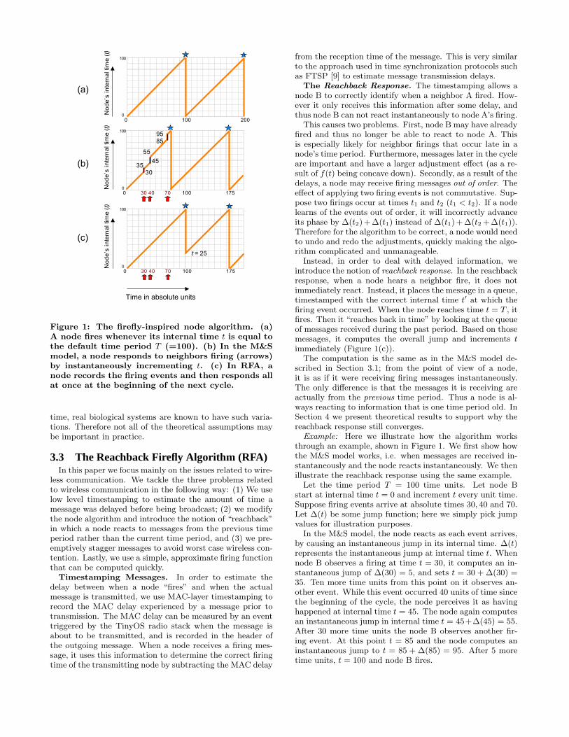
Each oscillator is characterized by a state variable s thatevolves according to s = f(φ) where f is the firing functionand φ is a phase variable representing where the oscillatoris in its cycle. For example, if an oscillator has finished 3/4of its cycle, then φ = 3/4. Thus φ ∈ [0, 1] and dφ/dt = 1/Twhere T is the period of the oscillator’s cycle. We assumethat the function f is monotonic, increasing, and concavedown. For our purposes, we choose f(φ) = ln(φ).

Now consider two oscillators A and B governed by f . Theycan be visualized as two points moving along the fixed curves = f(φ) at a constant horizontal velocity 1/T , as shown inFigure 2. When A reaches φ = 1 it will fire, and B will recordthe phase at which it hears A’s firing. In the RFA scheme,unlike the M&S model, B will not jump immediately uponhearing A’s fire; instead, B will record the time and thenexecute the appropriate jump after its next firing. The jumpis defined as ∆(φ) = g(f(φ) + ε) − φ, where g = f−1 andε � 1. For example, if B records φ1 as the time A fired,when B reaches φ = 1 it will fire and then jump forwardto φ = ∆(φ1). In the the RFA scheme, f(φ) = ln(φ) (andthus g(φ) = eφ), therefore ∆(φ) = (eε − 1)φ. The questionis whether the RFA scheme leads to synchrony.

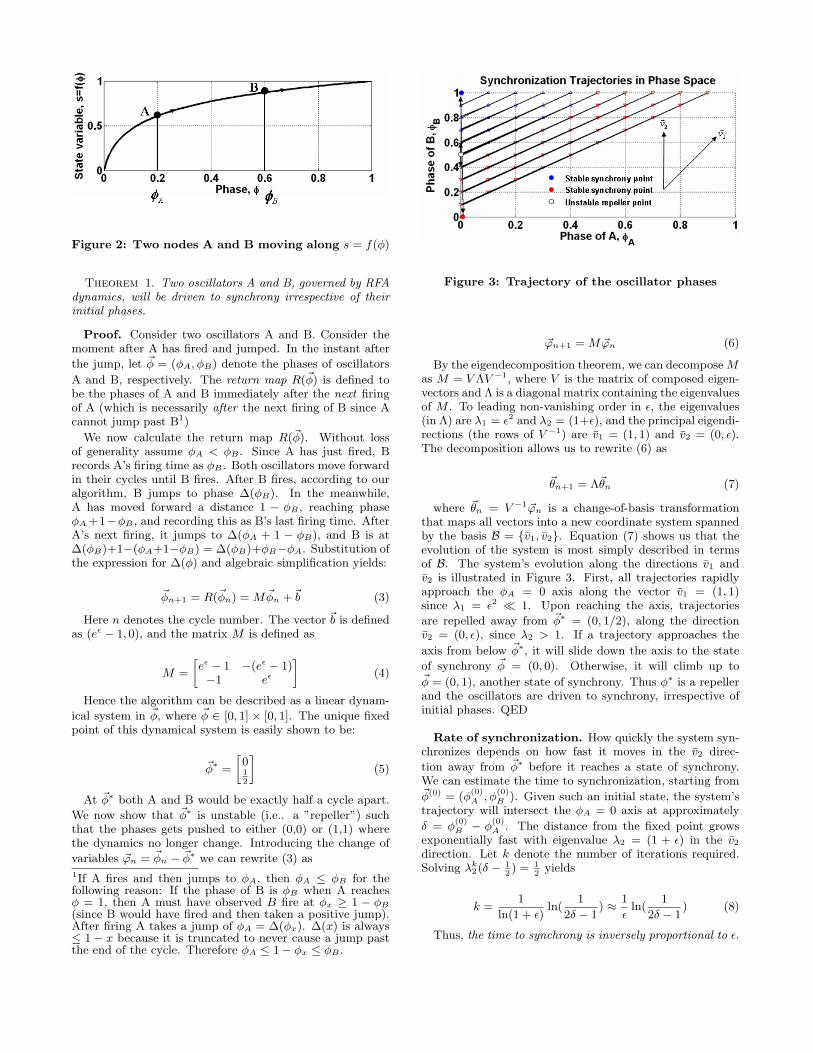
Figure 2: Two nodes A and B moving along s = f(φ)

Theorem 1. Two oscillators A and B, governed by RFAdynamics, will be driven to synchrony irrespective of theirinitial phases.

Proof. Consider two oscillators A and B. Consider themoment after A has fired and jumped. In the instant after

the jump, let ~φ = (φA, φB) denote the phases of oscillators

A and B, respectively. The return map R(~φ) is defined tobe the phases of A and B immediately after the next firingof A (which is necessarily after the next firing of B since Acannot jump past B1)

We now calculate the return map R(~φ). Without lossof generality assume φA < φB . Since A has just fired, Brecords A’s firing time as φB . Both oscillators move forwardin their cycles until B fires. After B fires, according to ouralgorithm, B jumps to phase ∆(φB). In the meanwhile,A has moved forward a distance 1 − φB , reaching phaseφA +1−φB , and recording this as B’s last firing time. AfterA’s next firing, it jumps to ∆(φA + 1 − φB), and B is at∆(φB)+1−(φA+1−φB) = ∆(φB)+φB−φA. Substitution ofthe expression for ∆(φ) and algebraic simplification yields:

~φn+1 = R(~φn) = M~φn +~b (3)

Here n denotes the cycle number. The vector ~b is definedas (eε − 1, 0), and the matrix M is defined as

M =

[eε − 1 −(eε − 1)−1 eε

](4)

Hence the algorithm can be described as a linear dynam-

ical system in ~φ, where ~φ ∈ [0, 1] × [0, 1]. The unique fixedpoint of this dynamical system is easily shown to be:

~φ∗ =

[012

](5)

At ~φ∗ both A and B would be exactly half a cycle apart.

We now show that ~φ∗ is unstable (i.e.. a ”repeller”) suchthat the phases gets pushed to either (0,0) or (1,1) wherethe dynamics no longer change. Introducing the change of

variables ~ϕn = ~φn − ~φ∗ we can rewrite (3) as

1If A fires and then jumps to φA, then φA ≤ φB for thefollowing reason: If the phase of B is φB when A reachesφ = 1, then A must have observed B fire at φx ≥ 1 − φB

(since B would have fired and then taken a positive jump).After firing A takes a jump of φA = ∆(φx). ∆(x) is always≤ 1− x because it is truncated to never cause a jump pastthe end of the cycle. Therefore φA ≤ 1− φx ≤ φB .

Figure 3: Trajectory of the oscillator phases

~ϕn+1 = M ~ϕn (6)

By the eigendecomposition theorem, we can decompose Mas M = V ΛV −1, where V is the matrix of composed eigen-vectors and Λ is a diagonal matrix containing the eigenvaluesof M . To leading non-vanishing order in ε, the eigenvalues(in Λ) are λ1 = ε2 and λ2 = (1+ε), and the principal eigendi-rections (the rows of V −1) are v̄1 = (1, 1) and v̄2 = (0, ε).The decomposition allows us to rewrite (6) as

~θn+1 = Λ~θn (7)

where ~θn = V −1~ϕn is a change-of-basis transformationthat maps all vectors into a new coordinate system spannedby the basis B = {v̄1, v̄2}. Equation (7) shows us that theevolution of the system is most simply described in termsof B. The system’s evolution along the directions v̄1 andv̄2 is illustrated in Figure 3. First, all trajectories rapidlyapproach the φA = 0 axis along the vector v̄1 = (1, 1)since λ1 = ε2 � 1. Upon reaching the axis, trajectories

are repelled away from ~φ∗ = (0, 1/2), along the directionv̄2 = (0, ε), since λ2 > 1. If a trajectory approaches the

axis from below ~φ∗, it will slide down the axis to the state

of synchrony ~φ = (0, 0). Otherwise, it will climb up to~φ = (0, 1), another state of synchrony. Thus φ∗ is a repellerand the oscillators are driven to synchrony, irrespective ofinitial phases. QED

Rate of synchronization. How quickly the system syn-chronizes depends on how fast it moves in the v̄2 direc-

tion away from ~φ∗ before it reaches a state of synchrony.We can estimate the time to synchronization, starting from~φ(0) = (φ

(0)A , φ

(0)B ). Given such an initial state, the system’s

trajectory will intersect the φA = 0 axis at approximately

δ = φ(0)B − φ

(0)A . The distance from the fixed point grows

exponentially fast with eigenvalue λ2 = (1 + ε) in the v̄2

direction. Let k denote the number of iterations required.Solving λk

2(δ − 12) = 1

2yields

k =1

ln(1 + ε)ln(

1

2δ − 1) ≈ 1

εln(

1

2δ − 1) (8)

Thus, the time to synchrony is inversely proportional to ε.

Note that these proofs are very similar to the two os-cillator case for Mirollo and Strogatz, and most likely canbe extended to n nodes. However extending these resultsto multi-hop topologies requires considerably more sophis-ticated analysis [8]. Instead we evaluate the algorithm insimulation for different n and network topologies.

5. EVALUATION TOOLS AND METRICSBoth our simulation and testbed experiments output a

series of node IDs and firing times. In order to discuss theaccuracy of the achieved synchronicity, it is necessary toidentify groups of nodes firing together.

For this purpose, we identify sets of node firings that fallwithin a prespecified time window. We call each clusterof node firings a group. Given a time window size w, theclustering algorithm outputs a series of firing groups thatmeet two constraints. First, every node firing event mustfall within exactly one group. Second, groups are chosen tocontain as many firing events as possible.

We define the group spread as the maximum time differ-ence between any two firings in the group. The time windowsize w represents the upper bound on the group spread.

5.1 Evaluation MetricsThe two evaluation metrics that we are concerned with

involve the amount of time until the system achieves syn-chronicity (if at all), and the accuracy of the achieved syn-chronicity.

Time To Sync: This is defined as the time that it takesall nodes to enter into a single group and stay withinthat group for 9 out of the last 10 firing iterations.The value chosen for the time window w does impactthe measured time to sync; a very small w will resultin a time to sync that is longer than with a larger w,because it takes longer for all nodes to join a firinggroup within a smaller time window. Also, as willbe discussed in the next sections, the simulator haslower time resolution than the testbed hardware whichmeans there is a limit on the accuracy it can achieve.Therefore, for the simulator we set w = 0.1sec and inthe real testbed we set w = 0.01sec.

50th and 90th Percentile Group Spread: Recall thatthe group spread measures the maximum time differ-ence between any two events in a firing group. Wewish to characterize the distribution of group spreadfor all groups after the system has achieved synchronic-ity. Although synchronicity may be achieved accordingto the time to sync metric above, we wish to avoid mea-suring group spread while the system is still settling.Given the first sync time ts and the time the experi-ment ends te, we calculate the group spread distribu-

tion across all groups in the interval [ts + (te−ts)2

, te].In this way we are measuring the distribution acrossall “tight” groups rather than settling effects. We plotthe 50th and 90th percentile of the distribution.

Lastly, we define the Firing Function Constant (FFC) tobe the value 1/ε, which is the main parameter in the RFAalgorithm. As discussed in Section 3.4, this parameter limitsthe response of a node to be at most T/FFC and thus thetime to synchronize is directly proportional to FFC.

6. SIMULATION RESULTSWe have implemented the Firefly algorithm in TinyOS [4]

using the TOSSIM [7] simulator environment. This simula-tor has several limitations. It does not model radio delaycorrectly, and nor does it take into account clock skew thatoccurs from variations in clock crystals in individual wirelesssensors. Despite these limitations, the simulator is useful forexploring the parameter space of our algorithm. This canhelp us determine optimal parameter settings for the algo-rithm on a real testbed as well as better understand theimpact of the parameter values on the level of synchronic-ity achieved. In our simulator experiments, we explore theimpact of varying:

1. Node topology: all-to-all where each node can com-municate with every other node, and a regular gridtopology where a node can directly exchange messageswith at most four other nodes.

2. Firing function constant value: ranging from 10-1000. Theoretically, the time to synchronize is propor-tional to the firing function constant value.

3. Number of nodes (n): We examine whether the im-pact of the firing function constant and node topologyvaries with the number of nodes. The size of the all-to-all topologies is varied between 2-20 nodes with 2node increments, and grid topologies are varied from16, 64, to 100 nodes.

All-to-all Topology Results. Figures 4(a) and 5 showthe results of simulations on the all-to-all topology. Weran simulations for firing function constant values (FFC)10,20,50,70,100,150,300,500,750 and 1000, repeating this com-bination for number of nodes ranging from 2-20 in 2 nodeincrements. For each parameter choice, we ran 10 simu-lations using different random seeds to start the nodes atdifferent times. Each experiment was run for 3600 secondsof simulation time. Also the time period T = 1sec for allexperiments.

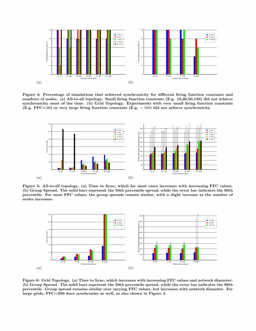
Fig. 4(a) shows the percentage of simulations that syn-chronized for a selection of parameter values. This percent-age represents the fraction of runs that achieved synchronic-ity out of the 10 total runs, for a given parameter choice of nand FFC. We can see that the FFC values displayed in thefigure (70,100,300,500 and 750) are fairly reliable since thesecases achieved synchronicity in a majority of the simulationruns. Most experiments with small firing function constants(10,20,50) did not achieve synchronicity. One likely rea-son for this behavior is that small FFC values lead nodesto make extremely large jumps, causing them to overshoot(see Section 3.4).

Fig. 5(a) shows the time to synchronize as a function ofFFC value and the number of nodes. The graph shows thatmost FFC constants work well. The time to sync increaseswith increasing FFC value but not beyond 400 time periods.There is no clear trend with increasing numbers of nodes,although small FFCs do not work as well with large numbersof nodes. This is possibly because the effect of overshoot isworsened when there are more neighbors (and thus moretotal firing events per cycle to react to).

Fig. 5(b) shows the corresponding group spreads. Formost FFC values and most n, the 90th percentile groupspread remains the same. The 50th percentile shows a slightincrease with increasing FFCs and a slight increase with

(a)

FF 70 FF 100 FF 300 FF 500 FF 750 FF 10000

20

40

60

80

100

Per

cent

age

Syn

chro

nize

d (%

)

Firing function constant

4 nodes

8 nodes

12 nodes

16 nodes

20 nodes

(b)

FF 20 FF 50 FF 100 FF 5000

20

40

60

80

100

Per

cent

age

Syn

chro

nize

d (%

)

Firing function constant

16 nodes

64 nodes

100 nodes

Figure 4: Percentage of simulations that achieved synchronicity for different firing function constants andnumbers of nodes. (a) All-to-all topology. Small firing function constants (E.g. 10,20,50,150) did not achievesynchronicity most of the time. (b) Grid Topology. Experiments with very small firing function constants(E.g. FFC=10) or very large firing function constants (E.g. > 500) did not achieve synchronicity.

(a)

FF 70 FF 100 FF 500 FF 750 FF 10000

200

400

600

800

1000

1200

Tim

e to

syn

c (s

ec)

Firing function constant

4 nodes

8 nodes

12 nodes

16 nodes

20 nodes

(b)

FF 70 FF 100 FF 500 FF 750 FF 10000

500

1000

1500

2000

2500

3000

3500

4000

4500

50th

and

90t

h pe

rcen

tile

grou

p sp

read

(use

c)

Firing function constant

4 nodes

8 nodes

12 nodes

16 nodes

20 nodes

Figure 5: All-to-all topology. (a) Time to Sync, which for most cases increases with increasing FFC values.(b) Group Spread. The solid bars represent the 50th percentile spread, while the error bar indicates the 90thpercentile. For most FFC values, the group spreads remain similar, with a slight increase as the number ofnodes increases

(a)

FF 20 FF 50 FF 100 FF 5000

200

400

600

800

1000

1200

Tim

e to

syn

c (s

ec)

Firing function constant

16 nodes

64 nodes

100 nodes

(b)

FF 20 FF 50 FF 100 FF 5000

5000

10000

15000

20000

25000

30000

35000

40000

50th

and

90t

h pe

rcen

tile

grou

p sp

read

(use

c)

Firing function constant

16 nodes

64 nodes

100 nodes

Figure 6: Grid Topology. (a) Time to Sync, which increases with increasing FFC values and network diameter.(b) Group Spread. The solid bars represent the 50th percentile spread, while the error bar indicates the 90thpercentile. Group spread remains similar over varying FFC values, but increases with network diameter. Forlarge grids, FFC=500 does synchronize as well, as also shown in Figure 4.

increasing numbers of nodes. However, the difference in thespreads is not large and thus group spreads remain fairlysimilar over all parameter values. The error bars for thisdata (not shown here) show that there is not much variationacross different experimental runs.

Grid Topology Results. Fig. 4(b) and 6 show the sim-ulation results for regular grid topologies of 4x4, 8x8, and10x10 nodes. Fig. 4(a) shows the percentage of cases thatsynchronized for a selection of parameter values. The resultsshow that FFC values in the range of 20-500 almost alwaysachieve synchronicity in a grid topology.

The behavior of nodes in a grid topology reflects the im-pact of network diameter on performance. Fig. 6 (a) showsthat large values of the firing function constant increase thetime taken to achieve synchronicity, and that this effect ismore pronounced for larger grids. Larger FFC values im-ply that nodes make smaller jumps and thus converge tosynchrony more slowly. For a given FFC, the time to syncalso increases slightly with network diameter, but not bymuch for the smaller FFC constants. The error bars for theFFC=500 simulations (not shown here) show that there isa large variation in time to sync and group spread acrossruns, most likely caused by the initial phase distribution ofnodes in the grid which can only be corrected slowly. Bar-ring that case, Fig. 6 (b) shows that the group spread doesnot vary significantly with FFC value. However there doesseem to be an increase in spread (i.e. decrease in accuracy)for larger grids, indicating that the network diameter mayhave an impact on how well the system can synchronize.

7. WIRELESS SENSOR NETWORKTESTBED EVALUATION

Having proven our algorithm correct in simple cases andexplored the parameter space using TOSSIM, we then testedRFA on a real sensor network testbed. The experimentscarried out on the 24-node indoor wireless sensor networktestbed, show the performance of our algorithm running onreal hardware, with a complex topology, and experiencingcommunication latencies over lossy asymmetric links. Thetable in Figure 10 summarizes our results, showing that RFAcan rapidly synchronize all the nodes to approx. 100 µsec.

This section is structured as follows. First, we describeour testbed environment, focusing on the significant ways inwhich the testbed differs from the TinyOS simulator. Wethen describe our use of FTSP to provide a common globaltime base for nodes participating in our experiments. Wethen discuss our experiments and results, and compare themto our expectation from theory and simulation.

7.1 Testbed EnvironmentOur experiments ran on MoteLab [16], a wireless sensor

network testbed consisting of 24 MicaZ motes distributedover one floor of our Computer Science and Electrical En-gineering building. The MicaZ motes have a 7.3MHz clock.Each device is attached to a Crossbow MIB600 interfacebackchannel board allowing remote reprogramming and datalogging. Messages sent to the nodes’ serial ports are loggedby a central server. Using this data-logging capability, nodesreport their firing times as well as information about firingmessages they observe. This information is then used toevaluate the performance of our algorithm, as well as betterunderstand its behavior.

Figure 7: Connectivity Map: The distribution andconnectivity of sensor nodes (detailed image athttp://motelab.eecs.harvard.edu/).

7.1.1 Network TopologyWe conducted our experiments on the most densely pop-

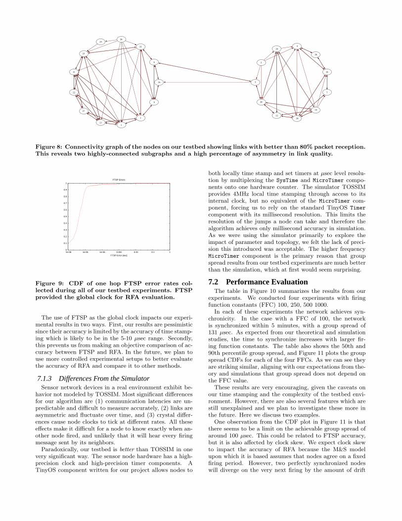
ulated floor, with 24 nodes. Statistics on message loss ratesare calculated periodically and tend to vary over time. Ex-amining the connectivity map and graph shown in Figures7 and 8, one can see that this is a complex multi-hop topol-ogy. The layout of the building produces two cliques ofnodes that are connected by high quality links (less than 20%message loss) and these cliques are connected by only a fewbridge nodes. Further examination of the cliques shows thata large fraction of the links are asymmetric in quality andsome nodes (e.g. 2, 26) may have no incoming links of goodquality. This type of complex topology is representative ofsensor networks distributed in a complex environment.

7.1.2 Time Stamping with FTSPIn order to evaluate the performance of RFA, we need to

time stamp the firing messages so that we can determine theaccuracy with which the firing phases align. However, thisproved to be difficult in our testbed environment. UnlikeTOSSIM, our sensor nodes do not have access to a globalclock. Furthermore, since they are distributed throughoutthe building, there is no single base station that can act asa global observer and provide a common time base [9]. Inan ironic way, evaluating RFA requires an independent andaccurate implementation of time stamping.

To address this difficulty we deployed the Flooding TimeSynchronization Protocol (FTSP) [9] described in Section2. FTSP provides nodes access to a stable global clock andallows them to time stamp events with precisions reportedin the tens of microseconds. We characterized the errorsin FTSP on our MoteLab topology in the following way.Nodes log all firing messages they hear from other nodesand the time stamp that FTSP assigned to them. For everyfiring message heard by more than two nodes, we computethe differences between the times that FTSP reported oneach node, taking the maximum difference between any twostamps. This is only done for messages where FTSP on boththe sender and receiver reported that the nodes were well-synchronized to the global clock. The cumulative distribu-tion frequency (CDF) of these errors for all of our testbedexperiments is shown in Figure 9. Note however that theFTSP errors are only calculated for nodes that are withinone hop of each other, therefore we do not know the errorin FTSP between two arbitrary nodes. Given this caveat,our results show that FTSP can quickly synchronize nodesto within one hop errors of tens of microseconds.

1

3

9

11

13

21

23

22

27

6

16

2

4

5

20

29

18

28

2412

19

7

2526

Figure 8: Connectivity graph of the nodes on our testbed showing links with better than 80% packet reception.This reveals two highly-connected subgraphs and a high percentage of asymmetry in link quality.

0

0.1

0.2

0.3

0.4

0.5

0.6

0.7

0.8

0.9

1

1e-06 1e-05 1e-04 0.001 0.01 0.1 1

FTSP Error (sec)

FTSP Errors

Figure 9: CDF of one hop FTSP error rates col-lected during all of our testbed experiments. FTSPprovided the global clock for RFA evaluation.

The use of FTSP as the global clock impacts our experi-mental results in two ways. First, our results are pessimisticsince their accuracy is limited by the accuracy of time stamp-ing which is likely to be in the 5-10 µsec range. Secondly,this prevents us from making an objective comparison of ac-curacy between FTSP and RFA. In the future, we plan touse more controlled experimental setups to better evaluatethe accuracy of RFA and compare it to other methods.

7.1.3 Differences From the SimulatorSensor network devices in a real environment exhibit be-

havior not modeled by TOSSIM. Most significant differencesfor our algorithm are (1) communication latencies are un-predictable and difficult to measure accurately, (2) links areasymmetric and fluctuate over time, and (3) crystal differ-ences cause node clocks to tick at different rates. All theseeffects make it difficult for a node to know exactly when an-other node fired, and unlikely that it will hear every firingmessage sent by its neighbors.

Paradoxically, our testbed is better than TOSSIM in onevery significant way. The sensor node hardware has a high-precision clock and high-precision timer components. ATinyOS component written for our project allows nodes to

both locally time stamp and set timers at µsec level resolu-tion by multiplexing the SysTime and MicroTimer compo-nents onto one hardware counter. The simulator TOSSIMprovides 4MHz local time stamping through access to itsinternal clock, but no equivalent of the MicroTimer com-ponent, forcing us to rely on the standard TinyOS Timer

component with its millisecond resolution. This limits theresolution of the jumps a node can take and therefore thealgorithm achieves only millisecond accuracy in simulation.As we were using the simulator primarily to explore theimpact of parameter and topology, we felt the lack of preci-sion this introduced was acceptable. The higher frequencyMicroTimer component is the primary reason that groupspread results from our testbed experiments are much betterthan the simulation, which at first would seem surprising.

7.2 Performance EvaluationThe table in Figure 10 summarizes the results from our

experiments. We conducted four experiments with firingfunction constants (FFC) 100, 250, 500 1000.

In each of these experiments the network achieves syn-chronicity. In the case with a FFC of 100, the networkis synchronized within 5 minutes, with a group spread of131 µsec. As expected from our theoretical and simulationstudies, the time to synchronize increases with larger fir-ing function constants. The table also shows the 50th and90th percentile group spread, and Figure 11 plots the groupspread CDFs for each of the four FFCs. As we can see theyare striking similar, aligning with our expectations from the-ory and simulations that group spread does not depend onthe FFC value.

These results are very encouraging, given the caveats onour time stamping and the complexity of the testbed envi-ronment. However, there are also several features which arestill unexplained and we plan to investigate these more inthe future. Here we discuss two examples.

One observation from the CDF plot in Figure 11 is thatthere seems to be a limit on the achievable group spread ofaround 100 µsec. This could be related to FTSP accuracy,but it is also affected by clock skew. We expect clock skewto impact the accuracy of RFA because the M&S modelupon which it is based assumes that nodes agree on a fixedfiring period. However, two perfectly synchronized nodeswill diverge on the very next firing by the amount of drift

FFC constant Time to 50th pct 90th pct Mean groupsync (sec) spread spread std dev

(µsec) (µsec)100 284.3 131.0 4664.0 410.4250 343.6 128.0 3605.0 572.2500 678.1 154.0 30236.0 1327.81000 1164.4 132.0 193.0 63.6

Figure 10: Summary of Testbed Results. Four ex-periments were run on the 24 node testbed, with dif-ferent firing function constants (where FFC = 1/ε)As expected, the time to synchronize increases withFFC. The 50th percentile group spread is similar forall four experiments.

0

0.1

0.2

0.3

0.4

0.5

0.6

0.7

0.8

0.9

1

1e-05 1e-04 0.001 0.01 0.1

Group Spread (sec)

Group Spread CDF

100250500

1000

Figure 11: CDF of RFA Group Spread. The fourdifferent firing function constants in the testbed ex-periments produce similar levels of synchronicity.

that exists in their clocks — introducing an error that is onthe order of the crystal accuracy. This causes the nodes toconstantly readjust their phases. Clock skew also impactsthe accuracy indirectly when nodes use the message delay(measured by the sender’s clock) to adjust their own phase.In the future we plan to investigate the effects of clock skewmore rigorously and look at alternate models of synchroniza-tion, such as synchronized clapping, where both frequencyand phase are adjusted.

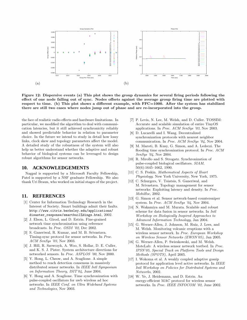
A second observation arises from looking at the groupspread over time. We observed that even after tight groupsform, occasionally disturbances still occur during the exper-iment. We refer to these as dispersive events. Figure 12 (a)shows an example of a dispersive event where the nodes fallout of phase and the system recovers from this impulse overthe next few firing periods. Figure 12 (b) shows a differ-ent time course with the occurrence of two dispersive eventswhich cause the group to spread over approximately 0.1 secrange. Note that these dispersive events are included inthe data in Table 10 and impact the 90th percentile groupspread. Analysis of the information collected during this ex-periment showed no clear reason for this spurious firing. Itis unlikely to be caused by the algorithm, since the extent ofdispersion is larger than the maximum jump possible giventhe FFC. What is encouraging is that the recovery from the100 msec range dispersive events takes only a few rounds toachieve, thus showing that the system can recover quickly

from perturbation. However, a more rigorous instrumenta-tion and experimentation setup will be required to pinpointthe causes behind this behavior.

8. COMPARISON TO OTHER METHODSCompared to algorithms such as RBS, TPSN and FTSP[2,

9, 3], the firefly-inspired algorithm represents a radicallydifferent approach. All of the nodes behave in a simpleand identical manner. There are no special nodes, such asthe root in TPSN or reference node in RBS, that need toelected. A node does not maintain any per-neighbor or per-link state; in fact it is completely agnostic to the identity ofits neighbors. The algorithm remains the same even if thetopology is multi-hop. There are no network-level datas-tructures, such as the spanning tree in TPSN, that mustbe re-established in case of topology change. As a resultof these properties, the algorithm is implicitly robust to thedisappearance of nodes and links. Lucarelli et al [8] haveshown that the algorithm works on time-varying topologies;our testbed results show that the algorithm performs welleven with asymmetric, lossy links. The inherent adaptivenature of such algorithms is one of the main attractions ofbiologically-inspired approaches.

Nevertheless, it is not yet clear whether such an algorithmwill be competitive to algorithms such as TPSN and FTSP,in terms of accuracy and overhead, and much work remainsto be done. In terms of accuracy, RFA achieves 100 µsecwhich is significantly less than the reported 10 µsec accu-racy of FTSP, although as discussed before it is difficult tomake a clear comparison because of the errors caused byusing FTSP as our evaluation clock. We believe that theaccuracy can be increased to tens of microseconds by elim-inating errors in our evaluation methodology and by usinga better optimized MAC-layer delay estimation (as used inFTSP [9]). However beyond that, the accuracy will still belimited by clock skew, as discussed in Section 7.2. We intendto investigate models that synchronize both phase and fre-quency, which would eliminate errors cause by clock skew.A second shortcoming of RFA is that the communicationoverhead is high. In particular, we choose T = 1 sec, unlikeFTSP which has a time period of 30 seconds. Assumingone could compensate for clock skew, the main limit on T isthe time taken to synchronize from startup. RFA takes ap-proximately 200 time periods to synchronize on MoteLab,which is significantly more than the diameter of the net-work. On the other hand, the system recovers quickly fromsmall dispersive events. One option would be to use a sim-ple mechanism, such as an initial flood, to bring all nodesto within a small phase difference quickly. Then RFA couldoperate at a much lower frequency to tighten the accuracyand maintain synchronicity. A different option is to allownodes to asynchronously backoff, or increase, their time pe-riod in multiples of T depending on whether they observemany out-of-phase firing events in their neighborhood. Thusnodes would self-adjust the overhead.

9. CONCLUSIONS AND FUTURE WORKIn this paper we have presented a decentralized algorithm

for synchronicity, based on a mathematical model of syn-chronicity achieved by biological systems. Our results showthat even though the theoretical models make simplifyingassumptions, this technique still works well and robustly in

(a)

-0.008

-0.006

-0.004

-0.002

0

0.002

0.004

0.006

0.008

1012 1014 1016 1018 1020 1022

Gro

up O

ffset

(se

c)

Group Fire Time (sec)

Group Dynamics Plot

12345679

11121316181920212223242526272830

(b)

0

0.2

0.4

0.6

0.8

1

1300 1400 1500 1600 1700 1800 1900 2000

Rel

ativ

e P

hase

(se

c)

Time (sec)

Phase Plot

12345679

11121316181920212223242526272830

Figure 12: Dispersive events (a) This plot shows the group dynamics for several firing periods following theeffect of one node falling out of sync. Nodes offsets against the average group firing time are plotted withrespect to time. (b) This plot shows a different example, with FFC=1000. After the system has stabilizedthere are still two cases where nodes jump out of phase and are re-incorporated into the group.

the face of realistic radio effects and hardware limitations. Inparticular, we modified the algorithm to deal with communi-cation latencies, but it still achieved synchronicity reliablyand showed predictable behavior in relation to parameterchoice. In the future we intend to study in detail how lossylinks, clock skew and topology parameters affect the model.A detailed study of the robustness of the system will alsohelp us better understand whether the adaptive and robustbehavior of biological systems can be leveraged to designrobust algorithms for sensor networks.

10. ACKNOWLEDGEMENTSNagpal is supported by a Microsoft Faculty Fellowship,

Patel is supported by a NSF graduate Fellowship. We alsothank Uri Braun, who worked on initial stages of the project.

11. REFERENCES[1] Center for Information Technology Research in the

Interest of Society. Smart buildings admit their faults.http://www.citris.berkeley.edu/applications/

disaster_response/smartbuil%dings.html, 2002.

[2] J. Elson, L. Girod, and D. Estrin. Fine-grainednetwork time synchronization using referencebroadcasts. In Proc. OSDI ’02, Dec 2002.

[3] S. Ganeriwal, R. Kumar, and M. B. Srivastava.Timing-sync protocol for sensor networks. In Proc.ACM SenSys ’03, Nov 2003.

[4] J. Hill, R. Szewczyk, A. Woo, S. Hollar, D. E. Culler,and K. S. J. Pister. System architecture directions fornetworked sensors. In Proc. ASPLOS ’00, Nov 2000.

[5] Y. Hong, L. Cheow, and A. Scaglione. A simplemethod to reach detection consensus in massivelydistributed sensor networks. In IEEE Intl Symposiumon Information Theory, ISIT’04, June 2004.

[6] Y. Hong and A. Scaglione. Time synchronization withpulse-coupled oscillators for uwb wireless ad hocnetworks. In IEEE Conf. on Ultra Wideband Systemsand Technologies, Nov 2003.

[7] P. Levis, N. Lee, M. Welsh, and D. Culler. TOSSIM:Accurate and scalable simulation of entire TinyOSapplications. In Proc. ACM SenSys ’03, Nov 2003.

[8] D. Lucarelli and I. Wang. Decentralizedsynchronization protocols with nearest neighborcommunication. In Proc. ACM SenSys ’04, Nov 2004.

[9] M. Maroti, B. Kusy, G. Simon, and A. Ledeczi. Theflooding time synchronization protocol. In Proc. ACMSenSys ’04, Nov 2004.

[10] R. Mirollo and S. Strogatz. Synchronization ofpulse-coupled biological oscillators. SIAM,50(6):1645–1662, 1990.

[11] C. S. Peskin. Mathematical Aspects of HeartPhysiology. New York University, New York, 1975.

[12] C. Schurgers, V. Tsiatsis, S. Ganeriwal, andM. Srivastava. Topology management for sensornetworks: Exploiting latency and density. In Proc.MobiHoc, 2002.

[13] G. Simon et al. Sensor network-based countersnipersystem. In Proc. ACM SenSys ’04, Nov 2004.

[14] N. Wakamiya and M. Murata. Scalable and robustscheme for data fusion in sensor networks. In IntlWorkshop on Biologically Inspired Approaches toAdvanced Information Technology, Jan 2004.

[15] G. Werner-Allen, J. Johnson, M. Ruiz, J. Lees, andM. Welsh. Monitoring volcanic eruptions with awireless sensor network. In Proc. European Workshopon Wireless Sensor Networks (EWSN’05), Jan 2005.

[16] G. Werner-Allen, P. Swieskowski, and M. Welsh.MoteLab: A wireless sensor network testbed. In Proc.IPSN’05, Special Track on Platform Tools and DesignMethods (SPOTS), April 2005.

[17] I. Wokoma et al. A weakly coupled adaptive gossipprotocol for application level active networks. In IEEEIntl Workshop on Policies for Distributed Systems andNetworks, 2002.

[18] W. Ye, J. Heidemann, and D. Estrin. Anenergy-efficient MAC protocol for wireless sensornetworks. In Proc. IEEE INFOCOM ’02, June 2002.