finite elements for electrodynamics and modal …...finite elements for electrodynamics and modal...
TRANSCRIPT

Finite Elements for Electrodynamicsand Modal Analysis of Dispersive Structures
André Nicolet, Guillaume DemésyATHENA Team
INSTITUT FRESNEL UMR 7249Aix-Marseille University, CNRS, ECM
Faculté de Saint Jérôme,13397 Marseille cedex 20, France
Mathematical and Numerical Modeling in Optics,IMA, Minneapolis, December 12 - 16, 2016
Finite Elements for Electrodynamics and Modal Analysis of Dispersive Structures 0 / 55

What do we want to do ?
To developNumerical models (using Finite Elements)
for Electrodynamics (to solve Maxwell’sequations)to provide Physical Understanding (modes,resonances, etc.)of Photonic Devices (taking into accountrealistic materials e.g. with time dispersivepermittivity)
Finite Elements for Electrodynamics and Modal Analysis of Dispersive Structures 0 / 55

What do we want to do ?
To developNumerical models (using Finite Elements)for Electrodynamics (to solve Maxwell’sequations)
to provide Physical Understanding (modes,resonances, etc.)of Photonic Devices (taking into accountrealistic materials e.g. with time dispersivepermittivity)
Finite Elements for Electrodynamics and Modal Analysis of Dispersive Structures 0 / 55

What do we want to do ?
To developNumerical models (using Finite Elements)for Electrodynamics (to solve Maxwell’sequations)to provide Physical Understanding (modes,resonances, etc.)
of Photonic Devices (taking into accountrealistic materials e.g. with time dispersivepermittivity)
Finite Elements for Electrodynamics and Modal Analysis of Dispersive Structures 0 / 55

What do we want to do ?
To developNumerical models (using Finite Elements)for Electrodynamics (to solve Maxwell’sequations)to provide Physical Understanding (modes,resonances, etc.)of Photonic Devices (taking into accountrealistic materials e.g. with time dispersivepermittivity)
Finite Elements for Electrodynamics and Modal Analysis of Dispersive Structures 0 / 55
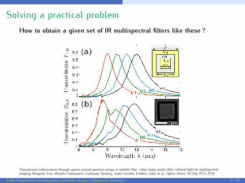
Solving a practical problemHow to obtain a given set of IR multispectral filters like these ?
Transmission enhancement through square coaxial aperture arrays in metallic film : when leaky modes filter infrared light for multispectralimaging, Benjamin Vial, Mireille Commandré, Guillaume Demésy, André Nicolet, Frédéric Zolla at al., Optics letters 39 (16), 4723-4726
Finite Elements for Electrodynamics and Modal Analysis of Dispersive Structures 1 / 55

Finite elements
Find u(R2 → R) of div(α grad v)) = f (+B.C.)Numerical solution using a piecewise 1st order polynomialapproximation function defined based on a triangular mesh - unknownsare nodal values en.wikipedia.org/wiki/Finite_element_method
Integration by parts lowers regularity requirement on the approximationfunction∫Ω
(div(α grad v))w dV = −
∫Ω
α grad v·gradw dV+∫∂Ω
wα grad v·ndS.
Finite Elements for Electrodynamics and Modal Analysis of Dispersive Structures 2 / 55

Electrodynamics
Maxwell’s equations curlH = J+ ∂tDcurlE = −∂tBdivD = ρdivB = 0
with Boundary Conditions (possibly →∞ such as the OutgoingWave Condition, Floquet-Bloch periodicity conditions...)and (Macroscopic) Constitutive Laws for Media relating D,H, J toE, B whathever "relating" means with D = εE, B = µH, J = σE assimplest cases...
Finite Elements for Electrodynamics and Modal Analysis of Dispersive Structures 3 / 55

Edge elementsFinite elements for 3D vectors fields (E, H, A...)
Unknown parameters are line integrals of the fieldalong the edges of the mesh...
... with vector-valued interpolation functions :Line integral of a "shape field" associated to an edge= 1 along this edge and is = 0 along the other edges.Picture from "Nedelec elements for computational electromagnetics", Per Jacobsson,June 5, 2007.2D example :
Finite Elements for Electrodynamics and Modal Analysis of Dispersive Structures 4 / 55

Edge elementsFinite elements for 3D vectors fields (E, H, A...)
Unknown parameters are line integrals of the fieldalong the edges of the mesh...... with vector-valued interpolation functions :Line integral of a "shape field" associated to an edge= 1 along this edge and is = 0 along the other edges.Picture from "Nedelec elements for computational electromagnetics", Per Jacobsson,June 5, 2007.2D example :
Finite Elements for Electrodynamics and Modal Analysis of Dispersive Structures 4 / 55
Edge elements
Some references :
H. Whitney : Geometric Integration Theory, Princeton U.P.(Princeton), 1957
J.C. Nedelec : "Mixed finite elements in IR3", Numer. Math., 35(1980), pp. 315-41
A. Bossavit, J.C. Vérité : "The TRIFOU Code : Solving the 3-DEddy-Currents Problem by Using H as State Variable", IEEETrans., MAG-19, 6 (1983), pp. 2465-70A. Bossavit : "Solving Maxwell’s Equations in a Closed Cavity, andthe Question of Spurious Modes", IEEE Trans. MAG-26, 2 (1990),pp. 702-5D. N. Arnold : "Differential complexes and numerical stability",Proceedings of the ICM, Beijing 2002, vol. 1, 137-157.
Finite Elements for Electrodynamics and Modal Analysis of Dispersive Structures 5 / 55

Edge elements
Some references :
H. Whitney : Geometric Integration Theory, Princeton U.P.(Princeton), 1957
J.C. Nedelec : "Mixed finite elements in IR3", Numer. Math., 35(1980), pp. 315-41A. Bossavit, J.C. Vérité : "The TRIFOU Code : Solving the 3-DEddy-Currents Problem by Using H as State Variable", IEEETrans., MAG-19, 6 (1983), pp. 2465-70
A. Bossavit : "Solving Maxwell’s Equations in a Closed Cavity, andthe Question of Spurious Modes", IEEE Trans. MAG-26, 2 (1990),pp. 702-5D. N. Arnold : "Differential complexes and numerical stability",Proceedings of the ICM, Beijing 2002, vol. 1, 137-157.
Finite Elements for Electrodynamics and Modal Analysis of Dispersive Structures 5 / 55

Edge elements
Some references :
H. Whitney : Geometric Integration Theory, Princeton U.P.(Princeton), 1957
J.C. Nedelec : "Mixed finite elements in IR3", Numer. Math., 35(1980), pp. 315-41A. Bossavit, J.C. Vérité : "The TRIFOU Code : Solving the 3-DEddy-Currents Problem by Using H as State Variable", IEEETrans., MAG-19, 6 (1983), pp. 2465-70A. Bossavit : "Solving Maxwell’s Equations in a Closed Cavity, andthe Question of Spurious Modes", IEEE Trans. MAG-26, 2 (1990),pp. 702-5
D. N. Arnold : "Differential complexes and numerical stability",Proceedings of the ICM, Beijing 2002, vol. 1, 137-157.
Finite Elements for Electrodynamics and Modal Analysis of Dispersive Structures 5 / 55

Edge elements
Some references :
H. Whitney : Geometric Integration Theory, Princeton U.P.(Princeton), 1957
J.C. Nedelec : "Mixed finite elements in IR3", Numer. Math., 35(1980), pp. 315-41A. Bossavit, J.C. Vérité : "The TRIFOU Code : Solving the 3-DEddy-Currents Problem by Using H as State Variable", IEEETrans., MAG-19, 6 (1983), pp. 2465-70A. Bossavit : "Solving Maxwell’s Equations in a Closed Cavity, andthe Question of Spurious Modes", IEEE Trans. MAG-26, 2 (1990),pp. 702-5D. N. Arnold : "Differential complexes and numerical stability",Proceedings of the ICM, Beijing 2002, vol. 1, 137-157.
Finite Elements for Electrodynamics and Modal Analysis of Dispersive Structures 5 / 55

Edge elements
Some references :H. Whitney : Geometric Integration Theory, Princeton U.P.(Princeton), 1957J.C. Nedelec : "Mixed finite elements in IR3", Numer. Math., 35(1980), pp. 315-41A. Bossavit, J.C. Vérité : "The TRIFOU Code : Solving the 3-DEddy-Currents Problem by Using H as State Variable", IEEETrans., MAG-19, 6 (1983), pp. 2465-70A. Bossavit : "Solving Maxwell’s Equations in a Closed Cavity, andthe Question of Spurious Modes", IEEE Trans. MAG-26, 2 (1990),pp. 702-5D. N. Arnold : "Differential complexes and numerical stability",Proceedings of the ICM, Beijing 2002, vol. 1, 137-157.
Finite Elements for Electrodynamics and Modal Analysis of Dispersive Structures 5 / 55

Modes
Modes are solutions without a source (in a boundeddomain)
L
Mode : Finite energy
T =2L
cω0 =
πc
L
Finite Elements for Electrodynamics and Modal Analysis of Dispersive Structures 6 / 55

Vector Eigenvalue Problem
Consider the following eigenvalue problem :
Find λ ∈ R and 0 6= u ∈ H(curl,Ω) such that :curl curl u = λu in Ω (∗)div u = 0 in Ωu× n|∂Ω = 0
The condition on the divergence is nearly redundant since taking thedivergence of (∗) gives λ div u = 0.For the non-zero eigenvalues this is equivalent to the null divergencecondition but not for the zero eigenvalue. In this case, λ = 0 would beassociated with the infinite dimensional eigenspace made of gradients :gradφ, φ ∈ H1(Ω).The null divergence condition eliminates such eigenvectors.
Finite Elements for Electrodynamics and Modal Analysis of Dispersive Structures 7 / 55
Vector Eigenvalue Problem with Edge Elements
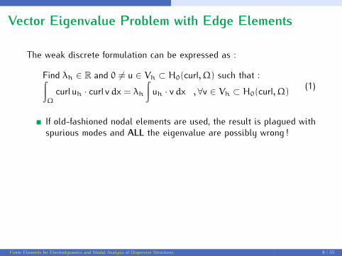
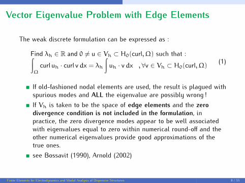
The weak discrete formulation can be expressed as :
Find λh ∈ R and 0 6= u ∈ Vh ⊂ H0(curl,Ω) such that :∫Ω
curl uh · curl vdx = λh∫uh · vdx , ∀v ∈ Vh ⊂ H0(curl,Ω)
(1)
If old-fashioned nodal elements are used, the result is plagued withspurious modes and ALL the eigenvalue are possibly wrong !
If Vh is taken to be the space of edge elements and the zerodivergence condition is not included in the formulation, inpractice, the zero divergence modes appear to be well associatedwith eigenvalues equal to zero within numerical round-off and theother numerical eigenvalues provide good approximations of thetrue ones.see Bossavit (1990), Arnold (2002)
Finite Elements for Electrodynamics and Modal Analysis of Dispersive Structures 8 / 55

Vector Eigenvalue Problem with Edge Elements
The weak discrete formulation can be expressed as :
Find λh ∈ R and 0 6= u ∈ Vh ⊂ H0(curl,Ω) such that :∫Ω
curl uh · curl vdx = λh∫uh · vdx , ∀v ∈ Vh ⊂ H0(curl,Ω)
(1)
If old-fashioned nodal elements are used, the result is plagued withspurious modes and ALL the eigenvalue are possibly wrong !If Vh is taken to be the space of edge elements and the zerodivergence condition is not included in the formulation, inpractice, the zero divergence modes appear to be well associatedwith eigenvalues equal to zero within numerical round-off and theother numerical eigenvalues provide good approximations of thetrue ones.
see Bossavit (1990), Arnold (2002)
Finite Elements for Electrodynamics and Modal Analysis of Dispersive Structures 8 / 55
Vector Eigenvalue Problem with Edge Elements
The weak discrete formulation can be expressed as :
Find λh ∈ R and 0 6= u ∈ Vh ⊂ H0(curl,Ω) such that :∫Ω
curl uh · curl vdx = λh∫uh · vdx , ∀v ∈ Vh ⊂ H0(curl,Ω)
(1)
If old-fashioned nodal elements are used, the result is plagued withspurious modes and ALL the eigenvalue are possibly wrong !If Vh is taken to be the space of edge elements and the zerodivergence condition is not included in the formulation, inpractice, the zero divergence modes appear to be well associatedwith eigenvalues equal to zero within numerical round-off and theother numerical eigenvalues provide good approximations of thetrue ones.see Bossavit (1990), Arnold (2002)
Finite Elements for Electrodynamics and Modal Analysis of Dispersive Structures 8 / 55

Vector Eigenvalue Problem with Edge Elements
gradPh ⊂ Vh with Ph = P1(Th), the Lagrange elements, andVh = N0(Th), the edge elements.This property is fundamental and can be encoded in a commutativediagram (interpolation and differential operator (grad) commute) .Choose v = gradϕ with ϕ in Ph. In this case∫Ω
curl uh · curl gradϕdx = λh∫Ω
uh · gradϕdx = 0 , ∀ϕ ∈ Ph
and for non-zero eigenvalues :∫Ω
uh · gradϕdx = 0 , ∀ϕ ∈ Ph , thedivergence of uh is weakly equal to zero.
Finite Elements for Electrodynamics and Modal Analysis of Dispersive Structures 9 / 55

Commutative Diagram : de Rham Complexand Discrete Fields
C∞(R3) grad−−−−→ [C∞(R3)]3 curl−−−−→ [C∞(R3)]3 div−−−−→ C∞(R3)
Π0h
y Π1h
y Π2h
y Π3h
yw0h
G−−−−→ w1hC−−−−→ w2h
D−−−−→ w3h
Figure – Commutative diagram for the discrete topological operators and theprojection operators on discrete fields. w0h are sets of nodal values, w1h are setsof line integrals along edges, w2h are sets of fluxes through facets, w3h are sets ofvolume integrals on tetrahedra, G is the node-edge incidence matrix, C is theedge-facet incidence matrix, D is the facet-tetrahedron incidence matrix, anincidence matrix has coefficients ∈ 1,−1, 0
Finite Elements for Electrodynamics and Modal Analysis of Dispersive Structures 10 / 55

Commutative Diagram : de Rham Complexand Edge Elements
C∞(R3) grad−−−−→ [C∞(R3)]3 curl−−−−→ [C∞(R3)]3 div−−−−→ C∞(R3)
Π0h
y Π1h
y Π2h
y Π3h
yW0h
grad−−−−→ W1h
curl−−−−→ W2h
div−−−−→ W3h
Figure – Commutative diagram for the discrete topological operators and theprojection operators on interpolated finite dimensional function spaces. W0
h
nodal elements , W1h edge elements,W2
h facet elements,W3h volume elements
Picture from Finite element exterior calculus : A new approach to the stability of finiteelements, Douglas N. Arnold, IMA talk, 2007.
Finite Elements for Electrodynamics and Modal Analysis of Dispersive Structures 11 / 55
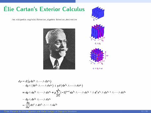
Élie Cartan’s Exterior Calculus/en.wikipedia.org/wiki/Exterior_algebra Exterior_derivative
Finite Elements for Electrodynamics and Modal Analysis of Dispersive Structures 12 / 55

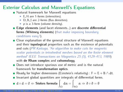
Exterior Calculus and Maxwell’s EquationsNatural framework for Maxwell equations
I E,H are 1-forms (intensities).I D,B, J are 2-forms (flux densities).I ρ is a 3-form (volume density).
Edge elements (and facet elements...) are discrete differentialforms (Whitney elements) (that make imposing boundaryconditions easy !).Clear explanation of the general structure of Maxwell equationsand their topological properties such as the existence of potentialsand cuts (PR Kotiuga, "An algorithm to make cuts for magneticscalar potentials in tetrahedral meshes based on the finite elementmethod" IEEE Transactions on Magnetics 25 (5), 4129-413, 1989)with de Rham complex and cohomology.Does not introduce spurious use of metric and is the naturalframework for transformation optics.Ready for higher dimensions (Einstein’s relativity) : F = E+B∧ dt.Invariant global quantities are integrals of differential forms.
d d = 0 ⇐ Stokes formula∫Ω
dα =
∫∂Ω
α ⇒ ∂ ∂ = ∅
Finite Elements for Electrodynamics and Modal Analysis of Dispersive Structures 13 / 55

Exterior Calculus and Maxwell’s EquationsNatural framework for Maxwell equations
I E,H are 1-forms (intensities).I D,B, J are 2-forms (flux densities).I ρ is a 3-form (volume density).
Edge elements (and facet elements...) are discrete differentialforms (Whitney elements) (that make imposing boundaryconditions easy !).
Clear explanation of the general structure of Maxwell equationsand their topological properties such as the existence of potentialsand cuts (PR Kotiuga, "An algorithm to make cuts for magneticscalar potentials in tetrahedral meshes based on the finite elementmethod" IEEE Transactions on Magnetics 25 (5), 4129-413, 1989)with de Rham complex and cohomology.Does not introduce spurious use of metric and is the naturalframework for transformation optics.Ready for higher dimensions (Einstein’s relativity) : F = E+B∧ dt.Invariant global quantities are integrals of differential forms.
d d = 0 ⇐ Stokes formula∫Ω
dα =
∫∂Ω
α ⇒ ∂ ∂ = ∅
Finite Elements for Electrodynamics and Modal Analysis of Dispersive Structures 13 / 55

Exterior Calculus and Maxwell’s EquationsNatural framework for Maxwell equations
I E,H are 1-forms (intensities).I D,B, J are 2-forms (flux densities).I ρ is a 3-form (volume density).
Edge elements (and facet elements...) are discrete differentialforms (Whitney elements) (that make imposing boundaryconditions easy !).Clear explanation of the general structure of Maxwell equationsand their topological properties such as the existence of potentialsand cuts (PR Kotiuga, "An algorithm to make cuts for magneticscalar potentials in tetrahedral meshes based on the finite elementmethod" IEEE Transactions on Magnetics 25 (5), 4129-413, 1989)with de Rham complex and cohomology.
Does not introduce spurious use of metric and is the naturalframework for transformation optics.Ready for higher dimensions (Einstein’s relativity) : F = E+B∧ dt.Invariant global quantities are integrals of differential forms.
d d = 0 ⇐ Stokes formula∫Ω
dα =
∫∂Ω
α ⇒ ∂ ∂ = ∅
Finite Elements for Electrodynamics and Modal Analysis of Dispersive Structures 13 / 55

Exterior Calculus and Maxwell’s EquationsNatural framework for Maxwell equations
I E,H are 1-forms (intensities).I D,B, J are 2-forms (flux densities).I ρ is a 3-form (volume density).
Edge elements (and facet elements...) are discrete differentialforms (Whitney elements) (that make imposing boundaryconditions easy !).Clear explanation of the general structure of Maxwell equationsand their topological properties such as the existence of potentialsand cuts (PR Kotiuga, "An algorithm to make cuts for magneticscalar potentials in tetrahedral meshes based on the finite elementmethod" IEEE Transactions on Magnetics 25 (5), 4129-413, 1989)with de Rham complex and cohomology.Does not introduce spurious use of metric and is the naturalframework for transformation optics.
Ready for higher dimensions (Einstein’s relativity) : F = E+B∧ dt.Invariant global quantities are integrals of differential forms.
d d = 0 ⇐ Stokes formula∫Ω
dα =
∫∂Ω
α ⇒ ∂ ∂ = ∅
Finite Elements for Electrodynamics and Modal Analysis of Dispersive Structures 13 / 55

Exterior Calculus and Maxwell’s EquationsNatural framework for Maxwell equations
I E,H are 1-forms (intensities).I D,B, J are 2-forms (flux densities).I ρ is a 3-form (volume density).
Edge elements (and facet elements...) are discrete differentialforms (Whitney elements) (that make imposing boundaryconditions easy !).Clear explanation of the general structure of Maxwell equationsand their topological properties such as the existence of potentialsand cuts (PR Kotiuga, "An algorithm to make cuts for magneticscalar potentials in tetrahedral meshes based on the finite elementmethod" IEEE Transactions on Magnetics 25 (5), 4129-413, 1989)with de Rham complex and cohomology.Does not introduce spurious use of metric and is the naturalframework for transformation optics.Ready for higher dimensions (Einstein’s relativity) : F = E+B∧ dt.
Invariant global quantities are integrals of differential forms.
d d = 0 ⇐ Stokes formula∫Ω
dα =
∫∂Ω
α ⇒ ∂ ∂ = ∅
Finite Elements for Electrodynamics and Modal Analysis of Dispersive Structures 13 / 55

Exterior Calculus and Maxwell’s EquationsNatural framework for Maxwell equations
I E,H are 1-forms (intensities).I D,B, J are 2-forms (flux densities).I ρ is a 3-form (volume density).
Edge elements (and facet elements...) are discrete differentialforms (Whitney elements) (that make imposing boundaryconditions easy !).Clear explanation of the general structure of Maxwell equationsand their topological properties such as the existence of potentialsand cuts (PR Kotiuga, "An algorithm to make cuts for magneticscalar potentials in tetrahedral meshes based on the finite elementmethod" IEEE Transactions on Magnetics 25 (5), 4129-413, 1989)with de Rham complex and cohomology.Does not introduce spurious use of metric and is the naturalframework for transformation optics.Ready for higher dimensions (Einstein’s relativity) : F = E+B∧ dt.Invariant global quantities are integrals of differential forms.
d d = 0 ⇐ Stokes formula∫Ω
dα =
∫∂Ω
α ⇒ ∂ ∂ = ∅
Finite Elements for Electrodynamics and Modal Analysis of Dispersive Structures 13 / 55

Electrodynamics
Maxwell’s equations (exterior calculus)dH = J+ ∂tDdE = −∂tBdD = ρdB = 0
Poynting identity
d(E∧H) = J∧ E+ E∧ ∂tD+H∧ ∂tB
These relations are metric free !
Finite Elements for Electrodynamics and Modal Analysis of Dispersive Structures 14 / 55

Metric
Distance, angle...Hodge star operator ∗ maps p-forms on (3− p)-forms.It is a linear algebraic operator that expresses the metric action onp-forms.Example of Euclidean metric in Cartesian coordinates : ∗dx = dy∧ dz
∗dy = dz∧ dx∗dz = dx∧ dy
This simplicity hides metric aspects in Cartesian coordinates butthe relations are more complicated with a general coordinatesystem...
Finite Elements for Electrodynamics and Modal Analysis of Dispersive Structures 15 / 55

Metric
... and electromagnetic constitutive laws !For example in free space :
D = ε0∗E
B = µ0∗HThe Hodge star operator is necessary to transform fields (1-forms)into flux densities (2-forms) !
Finite Elements for Electrodynamics and Modal Analysis of Dispersive Structures 16 / 55

Commutative Diagram : de Rham Complexand Whitney Forms
C∞(R3) d−−−−→ [C∞(R3)]3 d−−−−→ [C∞(R3)]3 d−−−−→ C∞(R3)
Π0h
y Π1h
y Π2h
y Π3h
yW0h
d−−−−→ W1h
d−−−−→ W2h
d−−−−→ W3h
Figure – Commutative diagram for the discrete topological operators and theprojection operators on interpolated finite dimensional function spaces. W0
h
nodal elements , W1h edge elements,W2
h facet elements,W3h volume elements
The role of the finite element interpolation together with the weakformulation (involving the scalar product) is to provide a numericalapproximation to the Hodge star operator !Remark : FDTD rather uses two dual rectangular and orthogonalmeshes.
Finite Elements for Electrodynamics and Modal Analysis of Dispersive Structures 17 / 55

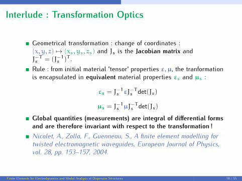
Interlude : Transformation Optics
Geometrical transformation : change of coordinates :(x, y, z) 7→ (xs, ys, zs) and Js is the Jacobian matrix andJ−Ts = (J−1s )T .
Rule : from initial material "tensor" properties ε,µ, the tranformationis encapsulated in equivalent material properties εs and µs :
εs = J−1s εJ−Ts det(Js)
µs = J−1s µJ−Ts det(Js)
Global quantities (measurements) are integral of differential formsand are therefore invariant with respect to the transformation !Nicolet, A., Zolla, F., Guenneau, S., A finite element modelling fortwisted electromagnetic waveguides, European Journal of Physics,vol. 28, pp. 153–157, 2004.
Finite Elements for Electrodynamics and Modal Analysis of Dispersive Structures 18 / 55

Interlude : Transformation Optics
Geometrical transformation : change of coordinates :(x, y, z) 7→ (xs, ys, zs) and Js is the Jacobian matrix andJ−Ts = (J−1s )T .Rule : from initial material "tensor" properties ε,µ, the tranformationis encapsulated in equivalent material properties εs and µs :
εs = J−1s εJ−Ts det(Js)
µs = J−1s µJ−Ts det(Js)
Global quantities (measurements) are integral of differential formsand are therefore invariant with respect to the transformation !
Nicolet, A., Zolla, F., Guenneau, S., A finite element modelling fortwisted electromagnetic waveguides, European Journal of Physics,vol. 28, pp. 153–157, 2004.
Finite Elements for Electrodynamics and Modal Analysis of Dispersive Structures 18 / 55
Interlude : Transformation Optics
Geometrical transformation : change of coordinates :(x, y, z) 7→ (xs, ys, zs) and Js is the Jacobian matrix andJ−Ts = (J−1s )T .Rule : from initial material "tensor" properties ε,µ, the tranformationis encapsulated in equivalent material properties εs and µs :
εs = J−1s εJ−Ts det(Js)
µs = J−1s µJ−Ts det(Js)
Global quantities (measurements) are integral of differential formsand are therefore invariant with respect to the transformation !Nicolet, A., Zolla, F., Guenneau, S., A finite element modelling fortwisted electromagnetic waveguides, European Journal of Physics,vol. 28, pp. 153–157, 2004.
Finite Elements for Electrodynamics and Modal Analysis of Dispersive Structures 18 / 55

From modes to quasimodes (also called quasinormalmodes (QNM) or leaky modes)
Quasimodes are solutions without a source in unboudeddomains corresponding to resonances...
L
Mode : Finite energy
ω0 =πc
L
L
leakage γ ∝ 1/τ
Quasimode : Infinite energy
ω = ω0 − iγ γ > 0
Finite Elements for Electrodynamics and Modal Analysis of Dispersive Structures 19 / 55

Leaky modes have an infinite power
Heuristics :Far enough, homogeneous medium : ∆u+ k2∞u = 0
Far field, outgoing wave :
e−i(ωt−k∞r)4πr
(or higher order multipole...)
ω is complex and k∞ = ω/c∞ is complex too...Im(ω) < 0 (leaky mode → energy loss in time)
=⇒ Im(k∞) < 0 (exponential divergence of eik∞r w.r.t. r) !
Finite Elements for Electrodynamics and Modal Analysis of Dispersive Structures 20 / 55

Leaky modes have an infinite power
Heuristics :Far enough, homogeneous medium : ∆u+ k2∞u = 0
Far field, outgoing wave :
e−i(ωt−k∞r)4πr
(or higher order multipole...)
ω is complex and k∞ = ω/c∞ is complex too...
Im(ω) < 0 (leaky mode → energy loss in time)
=⇒ Im(k∞) < 0 (exponential divergence of eik∞r w.r.t. r) !
Finite Elements for Electrodynamics and Modal Analysis of Dispersive Structures 20 / 55

Leaky modes have an infinite power
Heuristics :Far enough, homogeneous medium : ∆u+ k2∞u = 0
Far field, outgoing wave :
e−i(ωt−k∞r)4πr
(or higher order multipole...)
ω is complex and k∞ = ω/c∞ is complex too...Im(ω) < 0 (leaky mode → energy loss in time)
=⇒ Im(k∞) < 0 (exponential divergence of eik∞r w.r.t. r) !
Finite Elements for Electrodynamics and Modal Analysis of Dispersive Structures 20 / 55

Leaky modes have an infinite power
Heuristics :Far enough, homogeneous medium : ∆u+ k2∞u = 0
Far field, outgoing wave :
e−i(ωt−k∞r)4πr
(or higher order multipole...)
ω is complex and k∞ = ω/c∞ is complex too...Im(ω) < 0 (leaky mode → energy loss in time)
=⇒ Im(k∞) < 0 (exponential divergence of eik∞r w.r.t. r) !
Finite Elements for Electrodynamics and Modal Analysis of Dispersive Structures 20 / 55

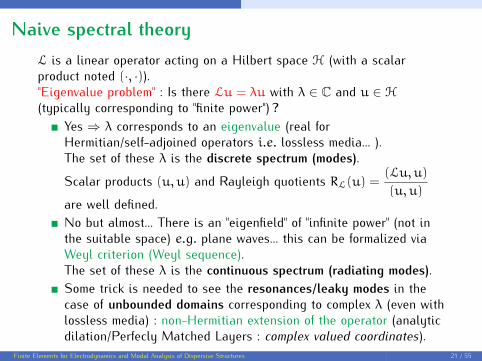
Naive spectral theoryL is a linear operator acting on a Hilbert space H (with a scalarproduct noted (·, ·))."Eigenvalue problem" : Is there Lu = λu with λ ∈ C and u ∈ H
(typically corresponding to "finite power") ?Yes ⇒ λ corresponds to an eigenvalue (real forHermitian/self-adjoined operators i.e. lossless media... ).The set of these λ is the discrete spectrum (modes).
Scalar products (u, u) and Rayleigh quotients RL(u) =(Lu, u)
(u, u)are well defined.
No but almost... There is an "eigenfield" of "infinite power" (not inthe suitable space) e.g. plane waves... this can be formalized viaWeyl criterion (Weyl sequence).The set of these λ is the continuous spectrum (radiating modes).Some trick is needed to see the resonances/leaky modes in thecase of unbounded domains corresponding to complex λ (even withlossless media) : non-Hermitian extension of the operator (analyticdilation/Perfecly Matched Layers : complex valued coordinates).
Finite Elements for Electrodynamics and Modal Analysis of Dispersive Structures 21 / 55

Naive spectral theoryL is a linear operator acting on a Hilbert space H (with a scalarproduct noted (·, ·))."Eigenvalue problem" : Is there Lu = λu with λ ∈ C and u ∈ H
(typically corresponding to "finite power") ?Yes ⇒ λ corresponds to an eigenvalue (real forHermitian/self-adjoined operators i.e. lossless media... ).The set of these λ is the discrete spectrum (modes).
Scalar products (u, u) and Rayleigh quotients RL(u) =(Lu, u)
(u, u)are well defined.No but almost... There is an "eigenfield" of "infinite power" (not inthe suitable space) e.g. plane waves... this can be formalized viaWeyl criterion (Weyl sequence).The set of these λ is the continuous spectrum (radiating modes).
Some trick is needed to see the resonances/leaky modes in thecase of unbounded domains corresponding to complex λ (even withlossless media) : non-Hermitian extension of the operator (analyticdilation/Perfecly Matched Layers : complex valued coordinates).
Finite Elements for Electrodynamics and Modal Analysis of Dispersive Structures 21 / 55
Naive spectral theoryL is a linear operator acting on a Hilbert space H (with a scalarproduct noted (·, ·))."Eigenvalue problem" : Is there Lu = λu with λ ∈ C and u ∈ H
(typically corresponding to "finite power") ?Yes ⇒ λ corresponds to an eigenvalue (real forHermitian/self-adjoined operators i.e. lossless media... ).The set of these λ is the discrete spectrum (modes).
Scalar products (u, u) and Rayleigh quotients RL(u) =(Lu, u)
(u, u)are well defined.No but almost... There is an "eigenfield" of "infinite power" (not inthe suitable space) e.g. plane waves... this can be formalized viaWeyl criterion (Weyl sequence).The set of these λ is the continuous spectrum (radiating modes).Some trick is needed to see the resonances/leaky modes in thecase of unbounded domains corresponding to complex λ (even withlossless media) : non-Hermitian extension of the operator (analyticdilation/Perfecly Matched Layers : complex valued coordinates).
Finite Elements for Electrodynamics and Modal Analysis of Dispersive Structures 21 / 55

Leaky modes and PMLs (Perfectly Matched Layers)
An extension of the (self-adjoined) operator, formally the same operatorbut acting on a larger domain (function space including "infinite powerleaky modes"), is required i.e. an non-Hermitian extension with complexeigenvalues...An interesting (theoretical and numerical) tool is provided by PML :J. Berenger (1994). "A perfectly matched layer for the absorption ofelectromagnetic waves". Journal of Computational Physics 114 (2) :185–200.In the harmonic, they can be viewed as a complex-valued change ofcoordinates : W. C. Chew and W. H. Weedon, A 3D perfectly matchedmedium from modified Maxwell’s equations with stretched coordinates,Microwave Optical Tech. Letters, vol. 7, no 13, 1994, p. 599-604.In this case, they are a useful tool to perform spectral analysis :Discretization of Continuous Spectra Based on Perfectly MatchedLayers, F. Olyslager, SIAM Journal on Applied Mathematics, Vol. 64,No. 4 (Apr. - Jun., 2004), pp. 1408-1433.
Finite Elements for Electrodynamics and Modal Analysis of Dispersive Structures 22 / 55
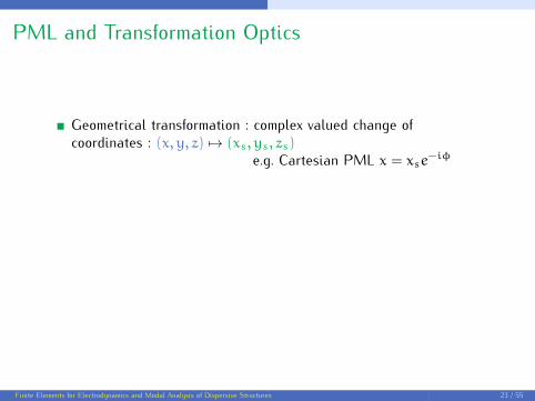
PML and Transformation Optics
Geometrical transformation : complex valued change ofcoordinates : (x, y, z) 7→ (xs, ys, zs)
e.g. Cartesian PML x = xse−iφ
Let k∞ = |k|e−iκ with κ > 0,we have k∞xs = |k|e−iκxeiφ = |k|xe−i(κ−φ)
=⇒ Im(k∞xs) = |k|xsin(φ− κ)Taking φ > κ to have Im(k∞xs) kills the exponential divergence ofeik∞xs w.r.t. xs.New scalar product (u, v)φ and a non-Hermitian extension Lφ ofthe operator can be defined...
Finite Elements for Electrodynamics and Modal Analysis of Dispersive Structures 23 / 55

PML and Transformation Optics
Geometrical transformation : complex valued change ofcoordinates : (x, y, z) 7→ (xs, ys, zs)
e.g. Cartesian PML x = xse−iφ
Let k∞ = |k|e−iκ with κ > 0,we have k∞xs = |k|e−iκxeiφ = |k|xe−i(κ−φ)
=⇒ Im(k∞xs) = |k|xsin(φ− κ)Taking φ > κ to have Im(k∞xs) kills the exponential divergence ofeik∞xs w.r.t. xs.
New scalar product (u, v)φ and a non-Hermitian extension Lφ ofthe operator can be defined...
Finite Elements for Electrodynamics and Modal Analysis of Dispersive Structures 23 / 55

PML and Transformation Optics
Geometrical transformation : complex valued change ofcoordinates : (x, y, z) 7→ (xs, ys, zs)
e.g. Cartesian PML x = xse−iφ
Let k∞ = |k|e−iκ with κ > 0,we have k∞xs = |k|e−iκxeiφ = |k|xe−i(κ−φ)
=⇒ Im(k∞xs) = |k|xsin(φ− κ)Taking φ > κ to have Im(k∞xs) kills the exponential divergence ofeik∞xs w.r.t. xs.New scalar product (u, v)φ and a non-Hermitian extension Lφ ofthe operator can be defined...
Finite Elements for Electrodynamics and Modal Analysis of Dispersive Structures 23 / 55
PML and Transformation Optics
Geometrical transformation : complex valued change of coordinates :(x, y, z) 7→ (xs, ys, zs) is turned into equivalent permittivity andpermeability εs and µs in the PML.
Point spectrum : Rayleigh quotients RL(u) =(Lu, u)
(u, u)are invariant
under the change of coordinates and modes are not modified !
Quasinormal Modes : Rayleigh quotients RLφ(u) =(Lu, u)φ(u, u)φ
becomes well defined for φ large enough and do not change forlarger φ : Quasimodes are unveiled !Continuous spectrum : Weyl sequences still correspond to kxs ∈ Rand therefore the k are multiplied by e−iφ : the continuousspectrum is rotated !
Finite Elements for Electrodynamics and Modal Analysis of Dispersive Structures 24 / 55

PML and Transformation Optics
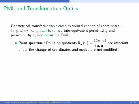
Geometrical transformation : complex valued change of coordinates :(x, y, z) 7→ (xs, ys, zs) is turned into equivalent permittivity andpermeability εs and µs in the PML.
Point spectrum : Rayleigh quotients RL(u) =(Lu, u)
(u, u)are invariant
under the change of coordinates and modes are not modified !
Quasinormal Modes : Rayleigh quotients RLφ(u) =(Lu, u)φ(u, u)φ
becomes well defined for φ large enough and do not change forlarger φ : Quasimodes are unveiled !
Continuous spectrum : Weyl sequences still correspond to kxs ∈ Rand therefore the k are multiplied by e−iφ : the continuousspectrum is rotated !
Finite Elements for Electrodynamics and Modal Analysis of Dispersive Structures 24 / 55

PML and Transformation Optics
Geometrical transformation : complex valued change of coordinates :(x, y, z) 7→ (xs, ys, zs) is turned into equivalent permittivity andpermeability εs and µs in the PML.
Point spectrum : Rayleigh quotients RL(u) =(Lu, u)
(u, u)are invariant
under the change of coordinates and modes are not modified !
Quasinormal Modes : Rayleigh quotients RLφ(u) =(Lu, u)φ(u, u)φ
becomes well defined for φ large enough and do not change forlarger φ : Quasimodes are unveiled !Continuous spectrum : Weyl sequences still correspond to kxs ∈ Rand therefore the k are multiplied by e−iφ : the continuousspectrum is rotated !
Finite Elements for Electrodynamics and Modal Analysis of Dispersive Structures 24 / 55

Rotation of continuous spectrum with PMLunveils leaky modes
An old technique in Quantum Mechanics : Balslev, E. ; Combes, J. M. Spectralproperties of many-body Schrödinger operators with dilatation-analyticinteractions. Communications in Mathematical Physics 22 (1971), no. 4,280–294. This is an EXACT modification of the initial problem, not anapproximation ! φ is the phase of the PML complex parameter s used for thecomplex stretch of the initial coordinates.
Finite Elements for Electrodynamics and Modal Analysis of Dispersive Structures 25 / 55

Bounded scatterer : (from Benjamin Vial Ph.D.)triangular rod εd = 13+ 0.2i
Finite Elements for Electrodynamics and Modal Analysis of Dispersive Structures 26 / 55

Bounded scatterer :triangular rod εd = 13+ 0.2i
0 0.5 1 1.5 2 2.5 3 3.5 4
x 1014
−2.5
−2
−1.5
−1
−0.5
0
x 1014
ω′ = Reω
ω′′=
Imω
continuous spectrum
PML modesleaky modes
1 2
3
Finite Elements for Electrodynamics and Modal Analysis of Dispersive Structures 27 / 55

Two leaky modes and one from the continuous spectrum(Bérenger mode). . .
−2 −1 0 1 2 3
ω1 = 1,77 · 1014 − 6,36 · 1012i rad.s−1
−4 −2 0 2 4
ω2 = 1,90 · 1014 − 1,01 · 1013i rad.s−1
−3 −2 −1 0 1 2 3
ω3 = 1,57 · 1014 − 1,29 · 1014i rad.s−1
Finite Elements for Electrodynamics and Modal Analysis of Dispersive Structures 28 / 55

InfraRed Multispectral Filter Conception using QNMHow to obtain a given set of IR multispectral filters like these ?
Transmission enhancement through square coaxial aperture arrays in metallic film : when leaky modes filter infrared light for multispectralimaging, Benjamin Vial, Mireille Commandré, Guillaume Demésy, André Nicolet, Frédéric Zolla at al., Optics letters 39 (16), 4723-4726
Finite Elements for Electrodynamics and Modal Analysis of Dispersive Structures 29 / 55

Filters conception
Modelling : parametric studySpectral parameters of the resonance as a function of the period d obtained fromcalculated transmission spectra (blue line) and extracted from the degeneratedeigenfrequencies (red crosses). (a) : resonant wavelength, (b) : spectral width. Electric (c)and magnetic (d) field maps of the leaky mode in the Oyz plane for d = 2.4µm.
Finite Elements for Electrodynamics and Modal Analysis of Dispersive Structures 30 / 55

Filters conception
λr targets : gives the conception parameter d
2 2.5 37
8
9
10
11
12
13
d (µm)
λr
(µm
)
M1
M2
M3
M4
Finite Elements for Electrodynamics and Modal Analysis of Dispersive Structures 31 / 55

Fabrication
Centre Interdisciplinaire des NAnosciences de Marseille (CINAM),UMR CNRS 7325, plateforme de lithographie électronique Planète
(CT-PACA, FEDER funding)
Finite Elements for Electrodynamics and Modal Analysis of Dispersive Structures 32 / 55

Multispectral chip
Focused beam, not polarizedSimulations
4 6 8 10 12 14 16 180
0.1
0.2
0.3
0.4
0.5
0.6
0.7
λ (µm)
T0,0
M1
M2
M3
M4
Measurements
4 6 8 10 12 14 16 180
0.1
0.2
0.3
0.4
0.5
0.6
0.7
λ (µm)
T0,0
M1
M2
M3
M4
Finite Elements for Electrodynamics and Modal Analysis of Dispersive Structures 33 / 55

Modes in presence highly dispersive permittivities
Handling frequency dispersion is naturally built-in when dealingwith direct time-harmonic problems : setting ω sets the value ofεr(ω) explicitly
What should be done in spectral problems, where ω is theeigenvalue ? This is of particular interest in the optical range :
I dispersion relations for waveguides, fibers, photonic crystals, . . .I study of resonant cavitiesI quasi-modal analyses
. . .where metals (Au, Ag, Al. . .) and semi-conductors (Si, GaAs,Ge. . .) exhibit resonant permittivities !
Finite Elements for Electrodynamics and Modal Analysis of Dispersive Structures 34 / 55

Why do we want the modes of dispersive structures ?example : frequency selective reflective surface with Au/Ag nano-particles 1
Structure :
Design - « optimization » :
Fabrication :
Characterisation :
1. Y. Brûlé, G. Demésy, A.-L. Fehrembach, B. Gralak, E. Popov, G. Tayeb, M. Grangier, D. Barat, H. Bertin, P. Gogol, and B. Dagens,« Design of metallic nanoparticle gratings for filtering properties in the visible spectrum », Appl. Opt. 54, 010359 (2015).
Finite Elements for Electrodynamics and Modal Analysis of Dispersive Structures 35 / 55

Causal permittivity models in very short...
Causal frequency dispersive materials ⇔ permittivity εr(ω) fulfillsKramers–Kronig relations.Causal materials can be modeled as a continuous sum of Lorentzresonances.Materials can be modeled as an infinite discrete sum of Lorentzresonances (still causal).On a limited spectral range, this sum can be truncated (still causal).In the visible range, 1 Lorentz + 1 Drude fits (and is still causal)for most metals and SC.
Finite Elements for Electrodynamics and Modal Analysis of Dispersive Structures 36 / 55

Permittivity models
Typically, εr writes as a rational function of ω :
Drude model : εr(ω) = ε∞ −ω2d
ω(ω+ iγd)
Lorentz model : εr(ω) = ε∞ −∆εω2l
ω2 + i γlω−ω2lDrude-Lorentz model :εr(ω) = ε∞ −
ω2dω(ω+ iγd)
−∆εω2l
ω2 + i γlω−ω2l. . .
In general : εr(ω) =N(ω)
D(ω)
arxiv.org/abs/1612.01876 "Extracting an accurate model for permittivity fromexperimental data : Hunting complex poles from the real line" MauricioGarcia-Vergara, Guillaume Demésy, Frédéric Zolla
Finite Elements for Electrodynamics and Modal Analysis of Dispersive Structures 37 / 55

The eigenvalue problem in a simple 2D case
We are looking for non trivial solutions of the source-free equation :
L2D(u) := −εr(x,ω)−1 div(µr−1 gradu) =
(ωc
)2u
i.e. the eigenvalues ωn and associated eigenvectors un of theoperator L2D
L2D(u) depends of ω we are looking for !
Let us compare two possible solutions :Physical linearization construction of an augmented system whereauxiliary fields are added to (E,H) 1 Numerical linearization
1. Y. Brûlé, B. Gralak, and G. Demésy, « Calculation and analysis of the complex bandstructure of dispersive and dissipative two-dimensional photonic crystals », J. Opt. Soc.Am. B 33, 691-702 (2016)
Finite Elements for Electrodynamics and Modal Analysis of Dispersive Structures 38 / 55

The polynomial eigenvalue problem (PEP)
With a Drude material εr(ω) = ε∞ −ω2d
ω(ω+ iγd), L2D(u) =
(ωc
)2u
becomes :
L2D3 (u)ω3 + L2D2 (u)ω2 + L2D1 (u)ω1 + L2D0 (u) = 0 ,
where :
L2D3 (u) := ε∞ u ,L2D2 (u) := i γd ε∞ u ,L2D1 (u) := −ω2d u+ c2 div
[µr
−1 gradu],
L2D0 (u) := i γd c2 div
[µr
−1 gradu].
This is a third order polynomial (nonlinear) EVP
Finite Elements for Electrodynamics and Modal Analysis of Dispersive Structures 39 / 55

Implementation
Solved as-is in GetDP (http://getdp.info, C. Geuzaine, Universitéde Liège) with two-level orthogonal Arnoldi eigensolver from SLEPc(http://slepc.upv.es, J. E. Roman, Universitat Politècnica deValència)
Formulation Name modal_o3; Type FemEquation;
Quantity Name u; Type Local; NameOfSpace H1;
Equation
Galerkin [ r0[] * DofGrad u, Grad u ]; ... Galerkin DtDof[ -I[] * c1[] * Dofu, u ]; ... Galerkin DtDof[ -I[] * r1[] * DofGrad u, Grad u ]; ... Galerkin DtDtDof[ - c2[] * Dofu, u ]; ... Galerkin DtDtDtDof[ I[] * c3[] * Dofu, u ]; ...
Finite Elements for Electrodynamics and Modal Analysis of Dispersive Structures 40 / 55
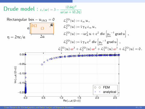
Drude model : εr(ω) = 3−(0.6η)2
ω(ω+ i0.2η)
Finite Elements for Electrodynamics and Modal Analysis of Dispersive Structures 41 / 55
Rectangular box – u|∂Ω = 0
η = 2πc/a
Ω∂Ω
yx
z
2a
a
0.0 0.5 1.0 1.5 2.0 2.5Reωna/(2πc)
−0.20
−0.15
−0.10
−0.05
0.00
Imω
na/(
2πc)
FEManalytical
L2D3 (u) := ε∞ u ,L2D2 (u) := i γd ε∞ u ,L2D1 (u) := −ω2d u+ c2 div
[µr
−1 gradu],
L2D0 (u) := i γd c2 div
[µr
−1 gradu],
L2D3 (u)ω3 + L2D2 (u)ω2 + L2D1 (u)ω1 + L2D0 (u) = 0 .

Lorentz model : εr(ω) = 3−4 (0.6η)2
ω2 + i 0.2ηω− (0.6η)2
Finite Elements for Electrodynamics and Modal Analysis of Dispersive Structures 41 / 55
Rectangular box – u|∂Ω = 0
η = 2πc/a
Ω∂Ω
yx
z
2a
a
0.2 0.4 0.6 0.8 1.0 1.2 1.4 1.6 1.8Reωna/(2πc)
−0.10
−0.08
−0.06
−0.04
−0.02
Imω
na/(
2πc)
FEManalytical
PEP writes as :4∑k=0
L2Dk (u)ωk = 0 .

Drude-Lorentz model : εr(ω) = 2−(0.5η)2
ω(ω+ i0.3η)−
2 (0.6η)2
ω2 + i 0.1ηω− (0.6η)2
Finite Elements for Electrodynamics and Modal Analysis of Dispersive Structures 41 / 55
Rectangular box – u|∂Ω = 0
η = 2πc/a
Ω∂Ω
yx
z
2a
a
0.4 0.6 0.8 1.0 1.2 1.4Reωna/(2πc)
−0.05
−0.04
−0.03
−0.02
−0.01
Imω
na/(
2πc)
FEManalytical
PEP writes as :5∑k=0
L2Dk (u)ωk = 0 .
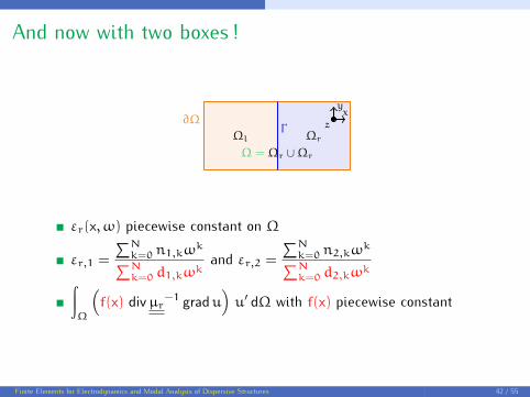
And now with two boxes !
ΓΩl Ωr
∂Ω
Ω = Ωr ∪Ωr
yx
z
εr(x,ω) piecewise constant on Ω
εr,1 =
∑Nk=0 n1,kω
k∑Nk=0 d1,kω
kand εr,2 =
∑Nk=0 n2,kω
k∑Nk=0 d2,kω
k∫Ω
(f(x) divµr
−1 gradu)u′ dΩ with f(x) piecewise constant
Finite Elements for Electrodynamics and Modal Analysis of Dispersive Structures 42 / 55

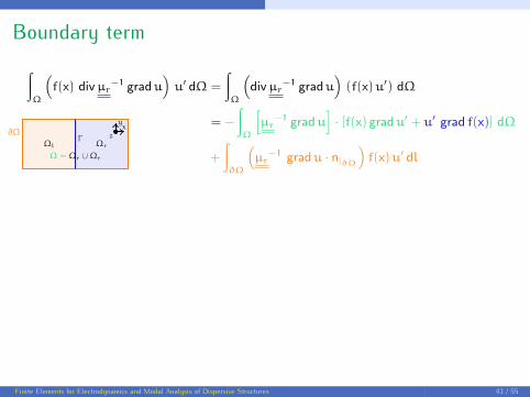
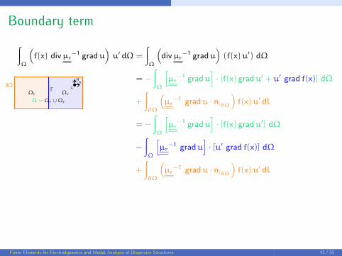
Boundary term
Finite Elements for Electrodynamics and Modal Analysis of Dispersive Structures 43 / 55
∫Ω
(f(x) divµr
−1 gradu)u′ dΩ =
∫Ω
(divµr
−1 gradu)(f(x)u′) dΩ
ΓΩl Ωr
∂Ω
Ω = Ωr ∪Ωr
yx
z
Boundary term
Finite Elements for Electrodynamics and Modal Analysis of Dispersive Structures 43 / 55
∫Ω
(f(x) divµr
−1 gradu)u′ dΩ =
∫Ω
(divµr
−1 gradu)(f(x)u′) dΩ
= −
∫Ω
[µr
−1 gradu]· [f(x) gradu′ + u′ grad f(x)] dΩ
+
∫∂Ω
(µr
−1 gradu · n|∂Ω)f(x)u′ dl
ΓΩl Ωr
∂Ω
Ω = Ωr ∪Ωr
yx
z
Boundary term
Finite Elements for Electrodynamics and Modal Analysis of Dispersive Structures 43 / 55
∫Ω
(f(x) divµr
−1 gradu)u′ dΩ =
∫Ω
(divµr
−1 gradu)(f(x)u′) dΩ
= −
∫Ω
[µr
−1 gradu]· [f(x) gradu′ + u′ grad f(x)] dΩ
+
∫∂Ω
(µr
−1 gradu · n|∂Ω)f(x)u′ dl
= −
∫Ω
[µr
−1 gradu]· [f(x) gradu′] dΩ
−
∫Ω
[µr
−1 gradu]· [u′ grad f(x)] dΩ
+
∫∂Ω
(µr
−1 gradu · n|∂Ω)f(x)u′ dl
ΓΩl Ωr
∂Ω
Ω = Ωr ∪Ωr
yx
z

Boundary term
Finite Elements for Electrodynamics and Modal Analysis of Dispersive Structures 43 / 55
∫Ω
(f(x) divµr
−1 gradu)u′ dΩ =
∫Ω
(divµr
−1 gradu)(f(x)u′) dΩ
= −
∫Ω
[µr
−1 gradu]· [f(x) gradu′ + u′ grad f(x)] dΩ
+
∫∂Ω
(µr
−1 gradu · n|∂Ω)f(x)u′ dl
= −
∫Ω
[µr
−1 gradu]· [f(x) gradu′] dΩ
−
∫Ω
[µr
−1 gradu]· [u′ grad f(x)] dΩ
+
∫∂Ω
(µr
−1 gradu · n|∂Ω)f(x)u′ dl
= −
∫Ω
[µr
−1 gradu]· [f(x) gradu′] dΩ
−
∫Ω
[µr
−1 gradu]·[u′ fjump
|ΓδΓn|Γ
]dΩ
+
∫∂Ω
(µr
−1 gradu · n|∂Ω)f(x)u′ dl
ΓΩl Ωr
∂Ω
Ω = Ωr ∪Ωr
yx
z

Boundary term
We need to impose jumps to f[µr
−1 gradu]· n|Γ , i.e.
jumps on the tangential trace of fH on ΓYet we do not have access to this quantity directly...
Finite Elements for Electrodynamics and Modal Analysis of Dispersive Structures 43 / 55
∫Ω
(f(x) divµr
−1 gradu)u′ dΩ =
∫Ω
(divµr
−1 gradu)(f(x)u′) dΩ
= −
∫Ω
[µr
−1 gradu]· [f(x) gradu′] dΩ
−
∫Γ
fjump|Γ
[µr
−1 gradu]· n|Γ u′dl
+
∫∂Ω
(µr
−1 gradu · n|∂Ω)f(x)u′ dl
ΓΩl Ωr
∂Ω
Ω = Ωr ∪Ωr
yx
z

Lagrange multipliers – Split one equation into three equations :
Finite Elements for Electrodynamics and Modal Analysis of Dispersive Structures 44 / 55
u1 = 0 on ∂Ω1 u2 = 0 on ∂Ω2
ΓΩ1 Ω2nΓ,1 nΓ,2
∂Ω1 ∂Ω2
N∑k=0
ωk
[∫Ω1
d1,k gradu1 · gradu′1 +ω2n1,k u1 u
′1dΩ1
]N∑k=0
ωk
[∫Ω2
d2,k gradu2 · gradu′2 +ω2n2,k u2 u
′2dΩ2
]
+
N∑k=0
ωj[∫Γ
dj,1λu′1dΓ
]−
N∑k=0
ωj[∫Γ
dj,2λu′2dΓ
]= 0 = 0
and∫Γ
(u1 − u2) λ′ dΓ = 0
λ is(µr
−1 gradu · nΓ)
, the discontinous tangential trace of H on one side of Γ .

Results for the two-boxSemi-analytical vs. FEM-augmented vs. FEM-polynomial
εr,1(ω) = 3−4 (0.6η)2
ω2 + i 0.2ηω− (0.6η)2with η = 2πc/a
εr,2(ω) = 2
0.2 0.4 0.6 0.8 1.0 1.2 1.4 1.6Real part !na/(2c)
0.10
0.08
0.06
0.04
0.02
0.00
Imag
inar
ypa
rt!
na/(
2c)
!1
analyticalFEM augmentedFEM polynomial
Finite Elements for Electrodynamics and Modal Analysis of Dispersive Structures 45 / 55

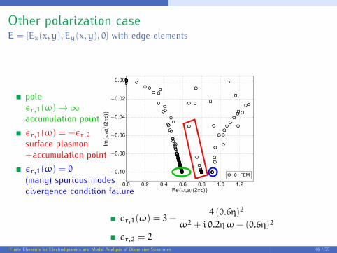
Other polarization caseE = [Ex(x, y), Ey(x, y), 0] with edge elements
Finite Elements for Electrodynamics and Modal Analysis of Dispersive Structures 46 / 55
εr,1(ω) = 3−4 (0.6η)2
ω2 + i 0.2ηω− (0.6η)2
εr,2 = 2
Other polarization caseE = [Ex(x, y), Ey(x, y), 0] with edge elements
Finite Elements for Electrodynamics and Modal Analysis of Dispersive Structures 46 / 55
εr,1(ω) = 3−4 (0.6η)2
ω2 + i 0.2ηω− (0.6η)2
εr,2 = 2
poleεr,1(ω)→∞accumulation pointεr,1(ω) = −εr,2surface plasmon+accumulation pointεr,1(ω) = 0(many) spurious modesdivergence condition failure

Other polarization caseE = [Ex(x, y), Ey(x, y), 0] with edge elements
Finite Elements for Electrodynamics and Modal Analysis of Dispersive Structures 46 / 55

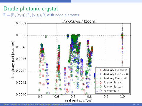
Drude photonic crystal
Single Drude resonance ε(ω) = 1−ω2p
ω(ω+ iγ)
With : ωpa2πc
= 1.1 ,γa
2πc= 0.05
material filling fraction = 0.65 for both and
r = 0.455 a for (w = 0.806 a) for
Finite Elements for Electrodynamics and Modal Analysis of Dispersive Structures 47 / 55

Drude photonic crystalE = [Ex(x, y), Ey(x, y), 0] with edge elements
Finite Elements for Electrodynamics and Modal Analysis of Dispersive Structures 48 / 55
Drude photonic crystalE = [Ex(x, y), Ey(x, y), 0] with edge elements
Finite Elements for Electrodynamics and Modal Analysis of Dispersive Structures 48 / 55
Conclusion and perspectives
Edge elements (and higher order generalizations) are a good toolfor the direct discretization of PDE operators of classicalelectrodynamics...Spectral problems for dispersive media – 2 linearization strategies :
I Augmented formalism – Auxiliary fieldsI Direct calculation of plasmonic resonances through solution of
polynomial eigenvalue problem with GetDP+SLEPc
Lagrange multipliers to deal with boundary terms in order to limitthe degree of the PEP in the case of several dispersive media.
To do :I Spectral transformations to explore specific regions of the spectrum.I Fix divergence condition failure (ε(ω) = 0).I Merge with PMLs for QNM of dispersive structures.I QNM expansion.I 3D . . .
Finite Elements for Electrodynamics and Modal Analysis of Dispersive Structures 49 / 55

Acknowledgment
F. Zolla, B. Vial, Y. Brûlé, B. Gralak @ Institut FresnelA.S. Bonnet and the POEMS Inria TeamThe Institute for Mathematics and Its ApplicationsC. Geuzaine, J. Roman, A. Bossavit, P.R. KotiugaThis work was supported by the ANR RESONANCE project, grantANR- 16-CE24-0013 of the French Agence Nationale de laRecherche (with P. Lalanne, C. Sauvan).and many others...THANK YOU FOR YOUR ATTENTION !
Finite Elements for Electrodynamics and Modal Analysis of Dispersive Structures 50 / 55

Supplementary Material
Finite Elements for Electrodynamics and Modal Analysis of Dispersive Structures 51 / 55

Tonti Diagram for Electrodynamics (in vector analysis)
Finite Elements for Electrodynamics and Modal Analysis of Dispersive Structures 52 / 55

two formulations for Ez(direct and Lagrange mult.)
0.0 0.5 1.0 1.5 2.0Reωn
−0.12
−0.10
−0.08
−0.06
−0.04
−0.02
0.00
Imω
n
Ez-pol for Dmodel - E out of plane - level setε∞1 = 3.00 ωd1 = 0.60 γd1 = 0.20 ωl1 = 0.00 γl1 = 0.00 ε1 = 0.00ε∞2 = 2.00 ωd2 = 0.00 γd2 = 0.00 ωl2 = 0.00 γl2 = 0.00 ε2 = 0.00
FEM weak form firstFEM lagrange mult
Finite Elements for Electrodynamics and Modal Analysis of Dispersive Structures 53 / 55

two formulations for Hz(Hz direct and Ex, Ey Lagrange mult.)
0.0 0.5 1.0 1.5 2.0−0.12
−0.10
−0.08
−0.06
−0.04
−0.02
0.00
ExEy-pol for Dmodel - E in plane - level setε∞1 = 3.00 ωd1 = 0.60 γd1 = 0.20 ωl1 = 0.00 γl1 = 0.00 δε1 = 0.00ε∞2 = 2.00 ωd2 = 0.00 γd2 = 0.00 ωl2 = 0.00 γl2 = 0.00 δε2 = 0.00
zero of ε1FEM weak form before - node Hz
FEM lagrange mult - edge (Ex , Ey)
Finite Elements for Electrodynamics and Modal Analysis of Dispersive Structures 54 / 55