finding small roots of polynomial equations using lattice basis
TRANSCRIPT
May 2009Kristian Gjøsteen, MATH
Master of Science in MathematicsSubmission date:Supervisor:
Norwegian University of Science and TechnologyDepartment of Mathematical Sciences
Finding Small Roots of PolynomialEquations Using Lattice BasisReduction
Ingeborg Sletta


Preface
With this thesis I end my 6 year stay here at NTNU. It have been some exciting andchallenging years where I have learned a lot. Socially I had some very nice years thanksto the class of LUR 2003.
Writing this thesis have been a challenging task that have required a lot of workalone. I have therefore appreciated my fellow students a lot for very meaningful breaksin the hall. I would specially like to thank Johan, Yvonne and Benedikte for LaTeX helpand motivation.
I would like to thank my supervisor Kristian Gjøsteen for introducing me to thisexciting field of mathematics, and for great guidance and help with this project.
I am grateful for my good friends who have been a great motivation and comfortduring these years. I would like to thank my parents, grandparents, my sister andbrother for being supportive and for giving me perspective and help. And I would liketo thank Jørgen for great support and help during these last two years.
Trondheim, May 29, 2009
Ingeborg Sletta
i

ii
Abstract
In 1996 Don Coppersmith used the Lenstra, Lenstra and Lovasz (LLL) algorithm to findsmall integer roots of polynomials. It was used on univariate modular equations andbivariate polynomial equations, and he proved that the method would find small roots,if they existed, in polynomial time.
In this thesis we look at the LLL-algorithm and how this can be used to solve uni-variate modular equations and bivariate polynomial equations. We talk briefly aboutcryptography and public-key cryptosystems, and we will present some theory about lat-tices. We will look in detail at Coppersmith’s method and show how it can be used toattack RSA encryption with a low exponent.
We will also look at improvements of this method done later by Howgrave-Grahamwhich simplifies the univariate case. In the end we give a small univariate example wherewe apply both Coppersmith’s and Howgrave-Graham’s method.
iii

iv

Contents
1 Introduction 1
2 Theory of lattices 32.1 Lattices . . . . . . . . . . . . . . . . . . . . . . . . . . . . . . . . . . . . . 32.2 Shortest Vector Problem and Closest Vector Problem . . . . . . . . . . . . 62.3 The LLL-algorithm . . . . . . . . . . . . . . . . . . . . . . . . . . . . . . . 62.4 Properties of the LLL-algorithm . . . . . . . . . . . . . . . . . . . . . . . 8
3 Cryptography 113.1 Knapsack cryptosystem . . . . . . . . . . . . . . . . . . . . . . . . . . . . 113.2 Finding roots . . . . . . . . . . . . . . . . . . . . . . . . . . . . . . . . . . 123.3 RSA cryptosystem . . . . . . . . . . . . . . . . . . . . . . . . . . . . . . . 12
4 Finding small roots of polynomial equations 154.1 Coppersmith - the univariate case . . . . . . . . . . . . . . . . . . . . . . . 16
4.1.1 Building the matrix M in the univariate case . . . . . . . . . . . . 174.1.2 Analysis of the determinant of M . . . . . . . . . . . . . . . . . . . 194.1.3 Finding the solution x0 . . . . . . . . . . . . . . . . . . . . . . . . 21
4.2 Coppersmith - the bivariate case . . . . . . . . . . . . . . . . . . . . . . . 234.2.1 Building the matrix M1 in the bivariate case . . . . . . . . . . . . 244.2.2 Analysis of the determinant . . . . . . . . . . . . . . . . . . . . . . 264.2.3 Finding the solution (x0, y0) . . . . . . . . . . . . . . . . . . . . . . 31
4.3 Howgrave-Graham - the univariate case . . . . . . . . . . . . . . . . . . . 314.3.1 Building the matrix M5 . . . . . . . . . . . . . . . . . . . . . . . . 324.3.2 Finding the solution x0 . . . . . . . . . . . . . . . . . . . . . . . . 33
5 An example 355.1 Coppersmith’s method . . . . . . . . . . . . . . . . . . . . . . . . . . . . . 355.2 Howgrave-Graham’s method . . . . . . . . . . . . . . . . . . . . . . . . . . 38
v

vi CONTENTS
Chapter 1
Introduction
The aim of this thesis is to understand the method described by Coppersmith on how tofind small roots of polynomial equations using lattice basis reduction. We will use Cop-persmith’s article [2] and go in detail in the univariate and the bivariate case. Howgrave-Graham [5] has improved the univariate case and we will look into his method as well.
In 1982 Lenstra, Lenstra and Lovasz developed the LLL-algorithm [6], which is anapproximation to the shortest vector problem. This algorithm takes a lattice basis asinput and converts it into a basis with short vectors that are nearly orthogonal andsorted by length. This has become an important algorithm with many applications. Wewill look at the algorithm and the properties of the basis returned by the algorithm.
In 1996 Coppersmith described how to use the LLL-algorithm on lattice bases to beable to find small roots of polynomials. Coppersmith makes a matrix that will span alattice, and this matrix consists among other things of the coefficients to our polynomial.After the matrix get the appropriate form we use the LLL-algorithm on it to get a LLL-reduced basis. We use this basis to create a new polynomial, that we can solve and thathave the same small roots as the original polynomial. This can be used to attack RSAcryptosystems with a low exponent.
Howgrave-Graham improved Coppersmiths univariate case by making a more directapproach. The matrix in this method is on a better form in the first place, so it demandsless computations. We use the LLL-algorithm in this case too, but we look at thefirst vector in the LLL-reduced basis instead of the last one as in Coppersmiths case.Howgrave-Graham proved that his and Coppersmith’s algorithm are equivalent, butHowgrave-Graham’s may be preferred for computational efficiency.
We start in Chapter 2 with some general theory about lattices and then we go throughthe LLL-algorithm and its properties. In Chapter 3 we look at the RSA cryptosystemwith the aim to motivate the reader on how Coppersmith’s method can be used toattack such systems. In Chapter 4 we go through the method of finding small rootsof polynomial equations as done by Coppersmith, and then Howgrave-Graham. In thelast chapter we show an example where we apply both Coppersmith’s and Howgrave-Graham’s method.
1

2 CHAPTER 1. INTRODUCTION
Chapter 2
Theory of lattices
2.1 Lattices
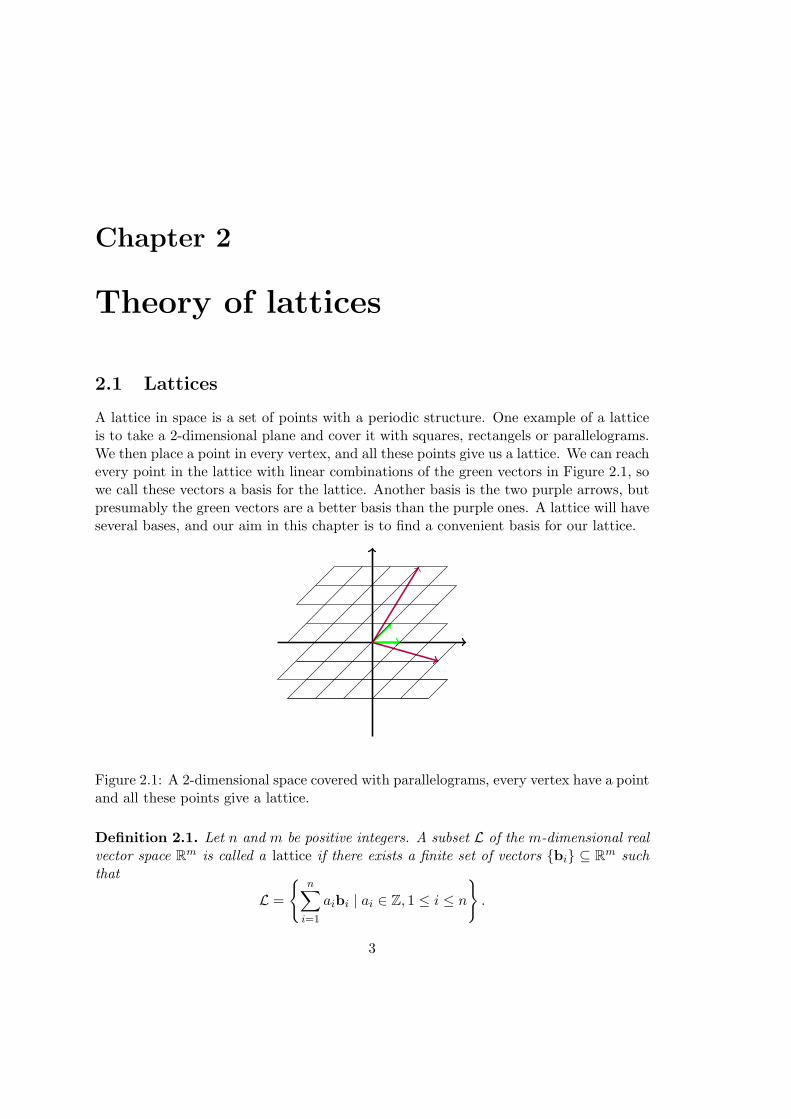
A lattice in space is a set of points with a periodic structure. One example of a latticeis to take a 2-dimensional plane and cover it with squares, rectangels or parallelograms.We then place a point in every vertex, and all these points give us a lattice. We can reachevery point in the lattice with linear combinations of the green vectors in Figure 2.1, sowe call these vectors a basis for the lattice. Another basis is the two purple arrows, butpresumably the green vectors are a better basis than the purple ones. A lattice will haveseveral bases, and our aim in this chapter is to find a convenient basis for our lattice.
Figure 2.1: A 2-dimensional space covered with parallelograms, every vertex have a pointand all these points give a lattice.
Definition 2.1. Let n and m be positive integers. A subset L of the m-dimensional realvector space Rm is called a lattice if there exists a finite set of vectors {bi} ⊆ Rm suchthat
L =
{n∑i=1
aibi | ai ∈ Z, 1 ≤ i ≤ n
}.
3

4 CHAPTER 2. THEORY OF LATTICES
We say that such a set {b1, ...,bn} is a basis if it spans L and is Z-linearly independent.We call n the rank of L, and m the dimension.
The lattice is a full-rank lattice if n = m. Given a n×m matrix B we can define
L = L(B) = {xB|x ∈ Zn} .
If we have a basis b1, . . . ,bn for L then we have a n×m matrix for L(B) = L,
B =
b1...
bn
,
where the bi’s are written as row vectors. The rank of the lattice is n which also is therank of the matrix B. The B matrix consists of the lattice basis as rows, and since thebasis vectors are linearly independent the row rank is n and so is the rank of the matrix.
Theorem 2.1. Let L be a finitely generated lattice over Z. Then all bases of L have thesame number of elements.
Proof. Let n < m and let b1, . . . ,bn and b′1, . . . ,b′m be two bases for L. We write
bi = a1ib′1 + · · ·+ amib′m, 1 ≤ i ≤ n
b′i = c1jb1 + · · ·+ cnjbn, 1 ≤ j ≤ m
Then
bi =n∑k=1
m∑j=1
ckjajibk
=n∑k=1
bkm∑j=1
ckjaji, 1 ≤ i ≤ n
thus because the bi’s are linearly independent
n∑k=1
bk
m∑j=1
ckjaji − λki
= 0
where
λki ={
0 i 6= k1 i = k
.
Let A = (aji) be a m× n matrix and C = (ckj) be a n×m matrix. This yields
CA =
c11 · · · c1m...
...cn1 · · · cnm
a11 · · · a1n
......
am1 · · · amn
= In
2.1. LATTICES 5
where In is a n × n identity matrix. Similarly AC = Im. Let A′ =(A 0
)and
C ′ =(C0
)be n × n augmented matrices, where each of the 0 blocks is a matrix of
appropriate size. Then
A′C ′ = In, C ′A′ =(In 00 0
).
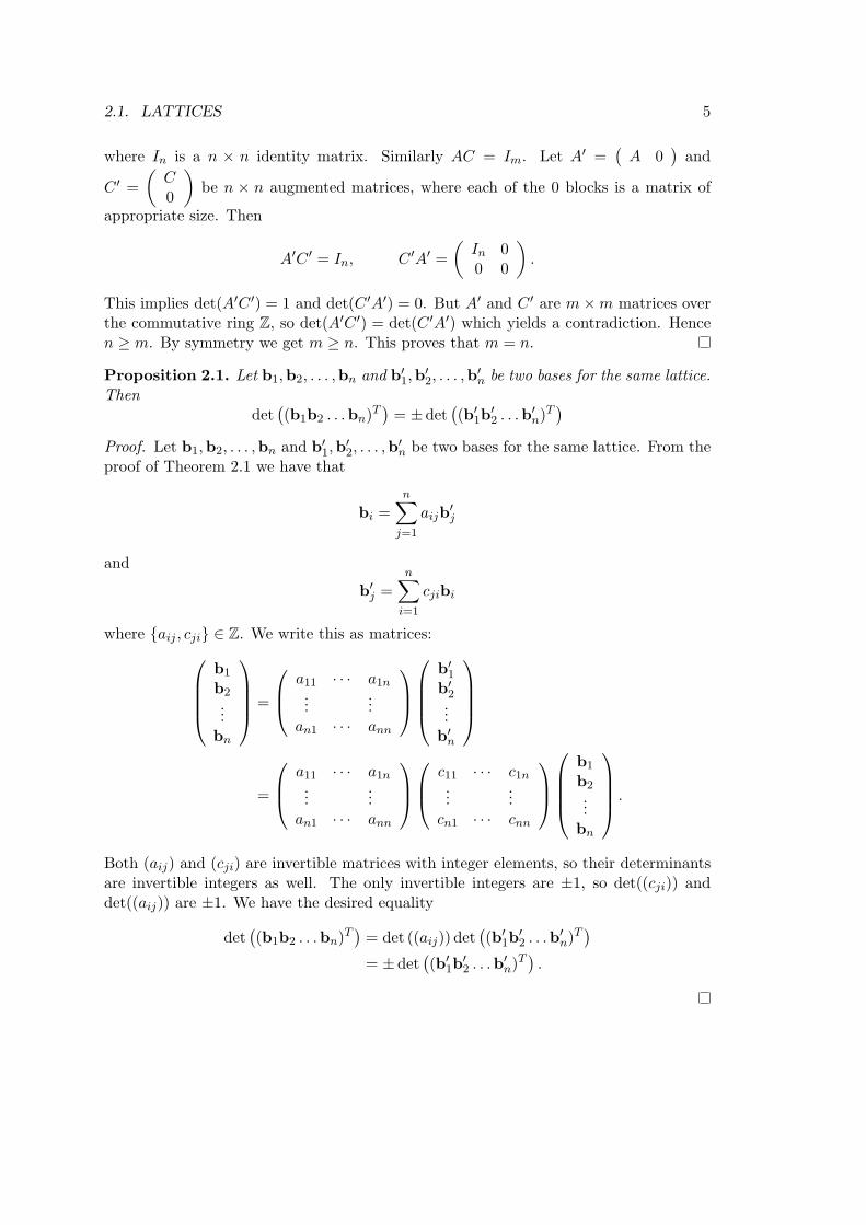
This implies det(A′C ′) = 1 and det(C ′A′) = 0. But A′ and C ′ are m×m matrices overthe commutative ring Z, so det(A′C ′) = det(C ′A′) which yields a contradiction. Hencen ≥ m. By symmetry we get m ≥ n. This proves that m = n.
Proposition 2.1. Let b1,b2, . . . ,bn and b′1,b′2, . . . ,b
′n be two bases for the same lattice.
Thendet((b1b2 . . .bn)T
)= ±det
((b′1b
′2 . . .b
′n)T)
Proof. Let b1,b2, . . . ,bn and b′1,b′2, . . . ,b
′n be two bases for the same lattice. From the
proof of Theorem 2.1 we have that
bi =n∑j=1
aijb′j
and
b′j =n∑i=1
cjibi
where {aij , cji} ∈ Z. We write this as matrices:b1
b2...
bn
=
a11 · · · a1n...
...an1 · · · ann
b′1b′2...
b′n
=
a11 · · · a1n...
...an1 · · · ann
c11 · · · c1n
......
cn1 · · · cnn
b1
b2...
bn
.
Both (aij) and (cji) are invertible matrices with integer elements, so their determinantsare invertible integers as well. The only invertible integers are ±1, so det((cji)) anddet((aij)) are ±1. We have the desired equality
det((b1b2 . . .bn)T
)= det ((aij)) det
((b′1b
′2 . . .b
′n)T)
= ±det((b′1b
′2 . . .b
′n)T).

6 CHAPTER 2. THEORY OF LATTICES
Let |·| denote the absolute value, (,) define the ordinary inner product on Rn and let‖·‖ define the ordinary Euclidean norm. We let the dot product of two vectors x and ybe denoted by x · y.
Definition 2.2. The determinant det(L) of a full rank lattice L(B) with basis b1, . . . ,bnis
det(L) = |detB| , where B =
b1...
bn
,
and the bi’s are written as row vectors.
We can now conclude that the determinant of the lattice is a positive real numberthat does not depend on the choice of the basis. It is positive since we take the absolutevalue.
2.2 Shortest Vector Problem and Closest Vector Problem
There are two central problems when studying a lattice, that is how to find the shortestvector in the lattice and how to find the closest vector to a point not in the lattice. Theseproblems are called the Shortest Vector Problem (SVP) and the Closest Vector Problem(CVP) and are two fundamental hard lattice problems. By a short vector we mean avector with small norm, so if a vector x is shorter than a vector y, then ‖x‖ < ‖y‖. TheSVP and CVP are defined as follows, where x ∈ L and x0 /∈ L:
SV P (L) = {x | x 6= 0, ∀y ∈ L : ‖x‖ ≤ ‖y‖}
CV P (L,x0) = {x | ∀y ∈ L : ‖x− x0‖ ≤ ‖y − x0‖}.
To solve SVP and CVP we want a basis whose basis elements are short and almostorthogonal. The next section give an algorithm that can find such a basis.
2.3 The LLL-algorithm
The Lenstra, Lenstra and Lovasz algorithm, usually named the LLL-algorithm, is anapproximation to the shortest vector problem. This algorithm was developed by A. K.Lenstra, H.W. Lenstra and L. Lovasz in 1982 [6].
The algorithm consists of a reduction step and a swap step. In the reduction step thebasis is reduced by the basis vectors with lower basis index. After all the vectors havebeen reduced, they get swapped. We would like to have the shortest element first andthe longest at the end, but we do not always need strict ordering. A δ decides how strictthe ordering is going to be, and δ is in the interval (1
4 , 1), where 1 would have given thestrict order.
The Gram-Schmidt orthogonalization process makes an inner product space basisorthogonal.

2.3. THE LLL-ALGORITHM 7
Definition 2.3. Given n linearly independent vectors b1, . . . ,bn ∈ Rn, the Gram-Schmidt orthogonalization of b1, . . . ,bn is defined by
bi = bi −i−1∑j=1
µi,jbj where µi,j =(bi, bj)(bj , bj)
.
We denote the Gram-Schmidt basis of b1, . . . ,bn by b1, . . . , bn .
The Gram-Schmidt of a basis element bi has shorter or equal length compared to bi,namely that ‖bi‖ ≤ ‖bi‖.
Definition 2.4. A basis B = {b1, ...,bn} ∈ Rn is a δ-LLL-Reduced Basis if the followingholds:
1. For all 1 ≤ j < i ≤ n we have |µi,j | ≤ 12 .
2. For all 1 ≤ i < n we have δ∥∥∥bi∥∥∥2
≤∥∥∥µi+1,ibi + bi+1
∥∥∥2.
The LLL-algorithm transforms an arbitrary basis into a δ-LLL-reduced one. Theinput to the algorithm is a lattice basis {b1, ...,bn} ∈ Zn. The output is a δ-LLL-reduced basis for the lattice. The algorithm is given in Figure 2.2, where d·c meansnearest integer.
Start: compute b1, ..., bnReduction step:
for i = 2 to n dofor j = i− 1 to 1 do
bi ← bi − ci,jbj where ci,j =⌈
(bi,bj)
(bj ,bj)
⌋Swap step:
if ∃i s.t. δ∥∥∥bi∥∥∥2
>∥∥∥µi+1,ibi + bi+1
∥∥∥2then
bi ↔ bi+1 for the smallest igo to start
Output b1, ...,bn
Figure 2.2: LLL-algorithm
We want to show that the algorithm gives us a reduced basis every time. We definethe potential of the lattice basis, a function mapping a lattice basis to a positive number.
Definition 2.5. Let B = {b1, . . . ,bn} be a lattice basis. The potential of B, denoted byDB is defined as
DB =n∏i=1
∥∥∥bi∥∥∥n−i+1=
n∏i=1
∥∥∥b1
∥∥∥∥∥∥b2
∥∥∥ · · · ∥∥∥bi∥∥∥ =n∏i=1
DB,i,
where DB,i = |det(Li)| and Li is defined as the lattice spanned by b1, . . . ,bi.
8 CHAPTER 2. THEORY OF LATTICES
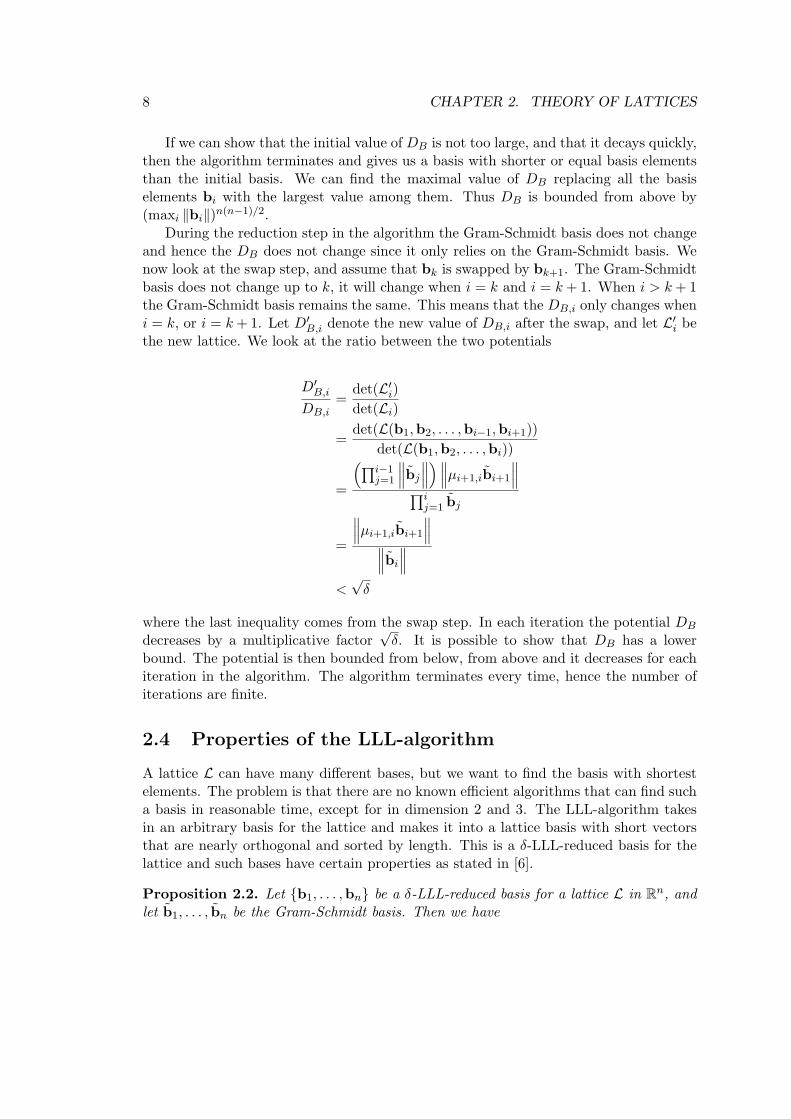
If we can show that the initial value of DB is not too large, and that it decays quickly,then the algorithm terminates and gives us a basis with shorter or equal basis elementsthan the initial basis. We can find the maximal value of DB replacing all the basiselements bi with the largest value among them. Thus DB is bounded from above by(maxi ‖bi‖)n(n−1)/2.
During the reduction step in the algorithm the Gram-Schmidt basis does not changeand hence the DB does not change since it only relies on the Gram-Schmidt basis. Wenow look at the swap step, and assume that bk is swapped by bk+1. The Gram-Schmidtbasis does not change up to k, it will change when i = k and i = k+ 1. When i > k+ 1the Gram-Schmidt basis remains the same. This means that the DB,i only changes wheni = k, or i = k+ 1. Let D′B,i denote the new value of DB,i after the swap, and let L′i bethe new lattice. We look at the ratio between the two potentials
D′B,iDB,i
=det(L′i)det(Li)
=det(L(b1,b2, . . . ,bi−1,bi+1))
det(L(b1,b2, . . . ,bi))
=
(∏i−1j=1
∥∥∥bj∥∥∥)∥∥∥µi+1,ibi+1
∥∥∥∏ij=1 bj
=
∥∥∥µi+1,ibi+1
∥∥∥∥∥∥bi∥∥∥<√δ
where the last inequality comes from the swap step. In each iteration the potential DB
decreases by a multiplicative factor√δ. It is possible to show that DB has a lower
bound. The potential is then bounded from below, from above and it decreases for eachiteration in the algorithm. The algorithm terminates every time, hence the number ofiterations are finite.
2.4 Properties of the LLL-algorithm
A lattice L can have many different bases, but we want to find the basis with shortestelements. The problem is that there are no known efficient algorithms that can find sucha basis in reasonable time, except for in dimension 2 and 3. The LLL-algorithm takesin an arbitrary basis for the lattice and makes it into a lattice basis with short vectorsthat are nearly orthogonal and sorted by length. This is a δ-LLL-reduced basis for thelattice and such bases have certain properties as stated in [6].
Proposition 2.2. Let {b1, . . . ,bn} be a δ-LLL-reduced basis for a lattice L in Rn, andlet b1, . . . , bn be the Gram-Schmidt basis. Then we have

2.4. PROPERTIES OF THE LLL-ALGORITHM 9
‖bj‖2 ≤ 2i−1 ‖bi‖2 for 1 ≤ j ≤ i ≤ n
‖b1‖ ≤ det(L)1/n2(n−1)/4.
Observe that b1 is a short element in the lattice. The first equation in Proposition2.2 give ‖b1‖2 ≤ 2n−1 ‖bn‖2. From this and the second equation of Proposition 2.2 itfollows that the last basis element bn satisfies∥∥∥bn∥∥∥ ≥ det(L)1/n2(n−1)/4. (2.1)
We do not necessarily find the shortest vector in the lattice, but we find a short one, soit is an approximation to the shortest vector problem. To solve SVP and CVP for anydimension is still hard.
Definition 2.6. A hyperplane in a n-dimensional space is the set of all y = (y0, . . . , yn)in the space which satisfies the equation
a0y0 + · · ·+ anyn = 0,
where not all ai are zero.
A hyperplane in a vector space is a vector subspace whose dimension is one less thanthe dimension of the whole vector space. We now look at some lemmas from Coppersmith[2], where b1,b2, . . . ,bn−1 is a δ-LLL-reduced basis.
Lemma 2.1. If a lattice element s satisfies ‖s‖ < det(L)1/n2(n−1)/4 then s lies in ahyperplane spanned by b1,b2, . . . ,bn−1.
Proof. A lattice element s can be expressed as s =∑n
i=1 aibi, where ai are integers. Thenorm of s is,
‖s‖ = ‖a1b1 + a2b2 + · · ·+ anbn‖ ≥ ‖anbn‖ = |an| ‖bn‖ ≥ |an| ‖bn‖ .
From (2.1) we have ‖bn‖ ≥ det(L)1/n2(n−1)/4 and we have that ‖s‖ < det(L)1/n2(n−1)/4
from Proposition 2.2. This gives us that s is shorter than the shortest orthogonal basiselement, then ‖s‖ < ‖bn‖. Thus we get that an must be zero and s must have dimensionn− 1 and therefore s lies in the hyperplane spanned by b1,b2, . . . ,bn−1.
In the further discussion we are not necessarily looking for the shortest nonzero vectorin the lattice but for a relatively short one, and Lemma 2.1 confines all such short vectorsto a hyperplane. In Lemma 2.2 we generalize this from a hyperplane to a subspace ofsmaller dimension.
Lemma 2.2. If a lattice element s satisfies ‖s‖ < ‖bi‖ for all i= k+1,. . . ,n, then s liesin a hyperplane spanned by b1,b2, . . . ,bk.

10 CHAPTER 2. THEORY OF LATTICES

Chapter 3
Cryptography
Cryptography is about communication when there are possible enemies around. The goalwith cryptography is to enable two persons, which we call Alice and Bob, to communicateover an insecure channel in such a way that an opponent, Oscar, cannot understandwhat is being said. We call the information that Alice wants to send Bob a plaintext.In advance Alice and Bob has secretly chosen a key K. This key then gives rise to anencryption rule eK and a decryption rule dK . Alice encrypts the plaintext before shesends it over the insecure channel, and when Bob receives it he decrypts the messageand gets the plaintext and the information Alice wanted to give him.
We call cryptosystems where eK and dK are the same, or where dK can easily bederived from eK , symmetric-key cryptosystems. In public-key cryptosystems on the otherhand, the encryption rule eK is a public key, and it is computationally infeasible to de-termine dK given eK . The public-key cryptography was first put forward in the openliterature by Diffie and Hellman in 1976. The theory was in reality developed years ear-lier. The security in public-key cryptography rests in different computational problems,but it can never provide unconditional security.
3.1 Knapsack cryptosystem
The knapsack encryption is a public key encryption scheme using a trap door function.The required trap door is obtained from the ancient knapsack puzzle: given the totalweight of a knapsack and the weight of individual objects, which objects are in the bag?This problem can be quite difficult to solve.
Public key systems based on the knapsack problem are generally suspected to beweaker than RSA, and some versions have already been broken. The Merkle-Hellmanknapsack encryption is based on the knapsack problem and was the first concrete realiza-tion of a public-key encryption scheme. It is therefore important for historical reasons.Many variations have been proposed, but most of them have been demonstrated to beinsecure, including the original.
The ancient knapsack problem is a subset sum problem, which is given by the follow-ing: given a set of positive integers {a1, a2, . . . , an} and a positive integer s, determine
11
12 CHAPTER 3. CRYPTOGRAPHY
whether or not there is a subset of the ai that sum to s. It can also be asked to actuallyfind a subset of the ai which sum to s, provided that such a subset exists.
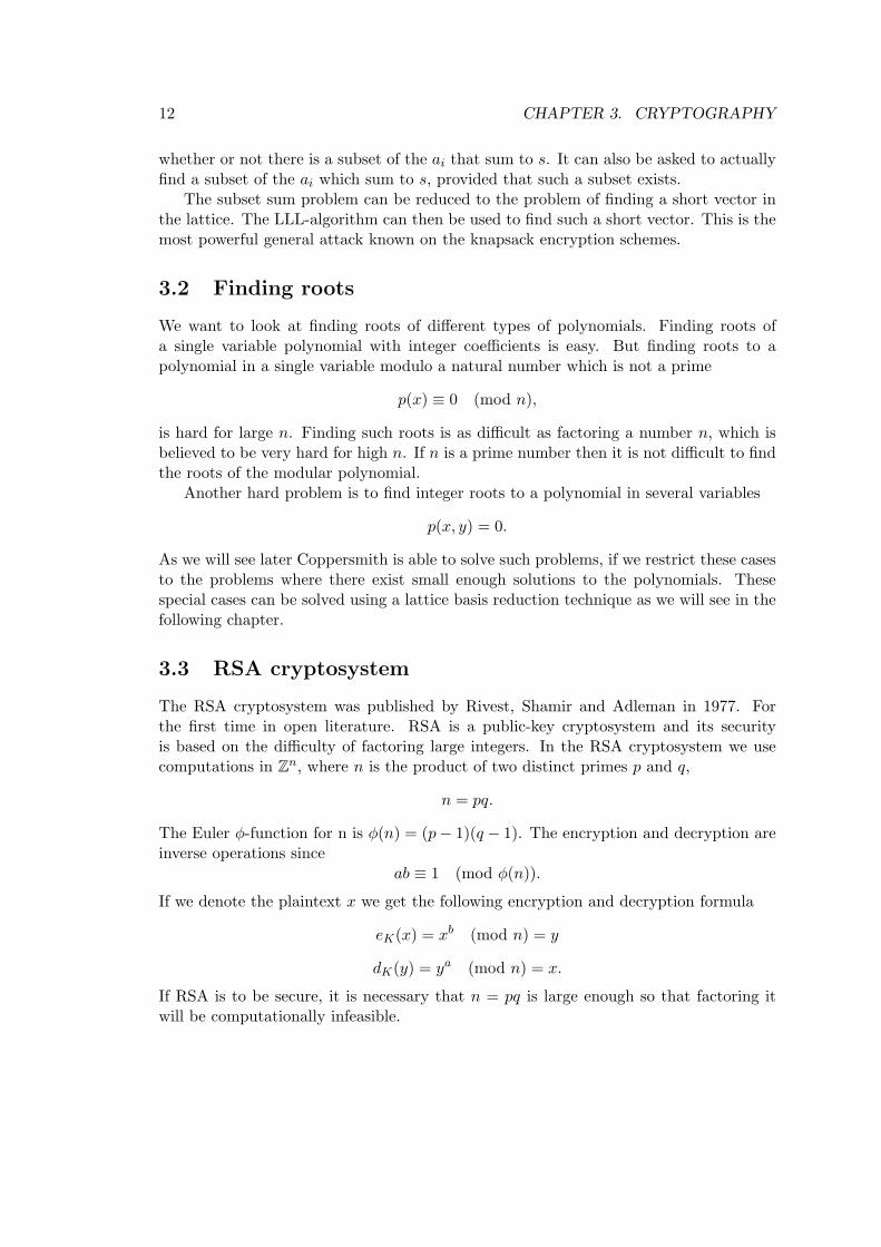
The subset sum problem can be reduced to the problem of finding a short vector inthe lattice. The LLL-algorithm can then be used to find such a short vector. This is themost powerful general attack known on the knapsack encryption schemes.
3.2 Finding roots
We want to look at finding roots of different types of polynomials. Finding roots ofa single variable polynomial with integer coefficients is easy. But finding roots to apolynomial in a single variable modulo a natural number which is not a prime
p(x) ≡ 0 (mod n),
is hard for large n. Finding such roots is as difficult as factoring a number n, which isbelieved to be very hard for high n. If n is a prime number then it is not difficult to findthe roots of the modular polynomial.
Another hard problem is to find integer roots to a polynomial in several variables
p(x, y) = 0.
As we will see later Coppersmith is able to solve such problems, if we restrict these casesto the problems where there exist small enough solutions to the polynomials. Thesespecial cases can be solved using a lattice basis reduction technique as we will see in thefollowing chapter.
3.3 RSA cryptosystem
The RSA cryptosystem was published by Rivest, Shamir and Adleman in 1977. Forthe first time in open literature. RSA is a public-key cryptosystem and its securityis based on the difficulty of factoring large integers. In the RSA cryptosystem we usecomputations in Zn, where n is the product of two distinct primes p and q,
n = pq.
The Euler φ-function for n is φ(n) = (p− 1)(q − 1). The encryption and decryption areinverse operations since
ab ≡ 1 (mod φ(n)).
If we denote the plaintext x we get the following encryption and decryption formula
eK(x) = xb (mod n) = y
dK(y) = ya (mod n) = x.
If RSA is to be secure, it is necessary that n = pq is large enough so that factoring itwill be computationally infeasible.

3.3. RSA CRYPTOSYSTEM 13
Example 3.1. Example of stereotyped message in RSAIn this example most of the message is fixed or “stereotyped”, we call this part of the
message F . An example of this F can be: “Todays password is...”. Let the plaintext mconsist of two pieces, x and F . The first piece F is known and is the fixed part of themessage. The second unknown piece x is the secret password, and the length of x is lessthan one-third the length of N . We use RSA encryption with an exponent of 3, so theciphertext c is given by
c = m3 = (F + x)3 (mod N).
We try to write this as a polynomial with x as the unknown, and we assume that weknow F , c and N . We then get
p(x) = (F + x)3 − c (mod N).
We want to find x0 so that
p(x0) = (F + x)3 − c = 0 (mod N).
If we can solve this polynomial for x0, then we will have recovered the secret message x.It is obvious that we can recover x if F = 0. We will show how to recover x for F 6= 0
in the following chapter.

14 CHAPTER 3. CRYPTOGRAPHY

Chapter 4
Finding small roots of polynomialequations using lattice basisreduction
In [1] and [2] Coppersmith describes how lattice reduction can be used to find small rootsof polynomial equations. It can be univariate modular equations, p(x) ≡ 0 (mod N),or bivariate polynomials, p(x, y) = 0. In both these cases the outline is the same, butthe bivariate case becomes more technical. Coppersmith makes a matrix that consistsof the coefficients to the polynomial we want to find the roots of, the modulus N in theunivariate case and some other factors. The rows of this matrix spans a lattice and wefind a sublattice of this lattice. We use a lattice basis reduction technique on vectorsin the sublattice, and find a hyperplane. This hyperplane contains all the short latticeelements. The equation of this hyperplane translates to a linear relation and then toa polynomial equation c(x0) = 0 or to c(x0, y0) = 0 over Z, where x0 or (x0, y0) area small root. In the univariate case we solve directly for x0. In the bivariate case wecombine p(x0, y0) and c(x0, y0) and solve. Coppersmith proved that at least one rootcan be found in polynomial time if we have a bound on the root we want to find.
Howgrave-Graham simplified Coppersmith’s algorithm for the univariate case bymaking a more direct approach. In the entries of the matrix consisting of the coefficientsof p(x) in Coppersmith’s case, Howgrave-Graham now uses entries that are multiples ofp(x) and N instead.
A simplification of the bivariate case was later proposed by Coron [3], but asymptot-ically its complexity was worse than Coppersmith’s method. But in [4] a new algorithmfor the bivariate integer case was put forward by Coron, this time with the same com-plexity as in Coppersmith’s method. We will not go into Coron’s algorithm here, butlook at the other three methods.
We restrict the problem of finding roots of the two polynomial equations describedfor the cases where there exist a solution small enough. We can solve these special casesusing a lattice basis reduction technique.
The idea is that we get a polynomial equation for example from RSA encryption, see
15
16 CHAPTER 4. FINDING SMALL ROOTS OF POLYNOMIAL EQUATIONS
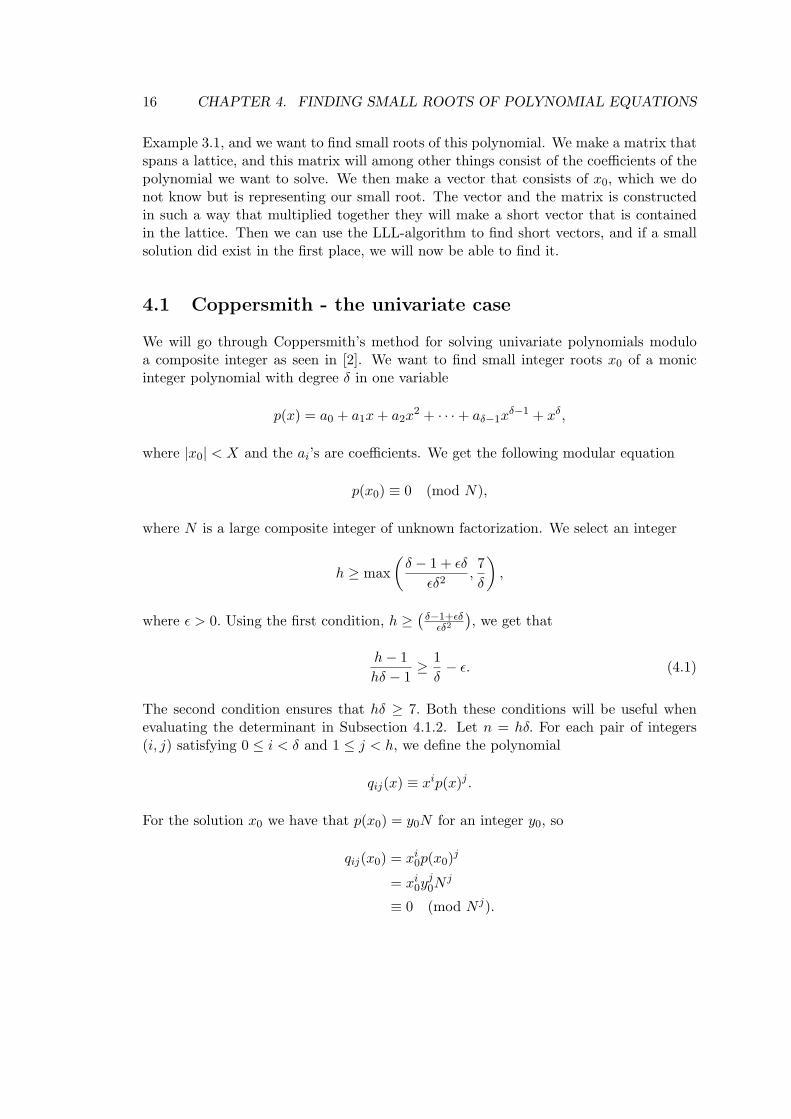
Example 3.1, and we want to find small roots of this polynomial. We make a matrix thatspans a lattice, and this matrix will among other things consist of the coefficients of thepolynomial we want to solve. We then make a vector that consists of x0, which we donot know but is representing our small root. The vector and the matrix is constructedin such a way that multiplied together they will make a short vector that is containedin the lattice. Then we can use the LLL-algorithm to find short vectors, and if a smallsolution did exist in the first place, we will now be able to find it.
4.1 Coppersmith - the univariate case
We will go through Coppersmith’s method for solving univariate polynomials moduloa composite integer as seen in [2]. We want to find small integer roots x0 of a monicinteger polynomial with degree δ in one variable
p(x) = a0 + a1x+ a2x2 + · · ·+ aδ−1x
δ−1 + xδ,
where |x0| < X and the ai’s are coefficients. We get the following modular equation
p(x0) ≡ 0 (mod N),
where N is a large composite integer of unknown factorization. We select an integer
h ≥ max(δ − 1 + εδ
εδ2,7δ
),
where ε > 0. Using the first condition, h ≥(δ−1+εδεδ2
), we get that
h− 1hδ − 1
≥ 1δ− ε. (4.1)
The second condition ensures that hδ ≥ 7. Both these conditions will be useful whenevaluating the determinant in Subsection 4.1.2. Let n = hδ. For each pair of integers(i, j) satisfying 0 ≤ i < δ and 1 ≤ j < h, we define the polynomial
qij(x) ≡ xip(x)j .
For the solution x0 we have that p(x0) = y0N for an integer y0, so
qij(x0) = xi0p(x0)j
= xi0yj0N
j
≡ 0 (mod N j).

4.1. COPPERSMITH - THE UNIVARIATE CASE 17
4.1.1 Building the matrix M in the univariate case
Coppersmith’s method consists of making a matrix where the rows of this matrix spansa lattice. The matrix M of size (2hδ − δ)× (2hδ − δ) is upper triangular and is definedto be
M =(A C0 D
),
where we have divided M into 4 blocks. The upper left (hδ) × (hδ) block A is a diagonalmatrix where the g’th entry on the diagonal is X−g
hδ where g starts from zero and goesto hδ− 1, 0 ≤ g < hδ. The upper right block C is a matrix of size (hδ)× (hδ− δ), wherethe rows are indexed by g, and the columns by γ(i, j). The γ-function takes in values iand j where 0 ≤ i < δ and 1 ≤ j < h, and
γ(i, j) = hδ + i+ (j − 1)δ.
The γ-function will give values in the following interval hδ ≤ γ(i, j) < 2hδ − δ. Theelement in C at the entry (g, γ(i, j)) is the coefficient of xg in the polynomial qij(x). Thelower left (hδ−δ)×(hδ−δ) block is a zero matrix, and the lower right (hδ−δ)×(hδ−δ)block D is a diagonal matrix where the value on the diagonal in column number γ(i, j)is N j .
We construct a vector r whose elements consist of powers of the desired integersolution x0 and the integer y0,
r(x0) = r =(
1, x0, x20, . . . , x
hδ−10 ,−y0,−x0y0, . . . ,−xδ−1
0 y0,−y20, x0y
20, . . . ,−xδ−1
0 yh−10
)where the first hδ entries are of the form
rg = xg0
for 0 ≤ g < hδ. The rest of the hδ − δ entries can be written as
rγ(i,j) = −xi0yj0
for hδ ≤ γ(i, j) < 2hδ − δ. We can write r as
r = (rg, rγ(i,j)).
We emphasize that we still do not know x0 or y0, but we know that they exist byassumption.
This r vector is constructed in such a way that multiplied with the matrix M we geta vector s with 0’s in the last entries,
s(x0) = s =
(1√hδ,
(x0X )√hδ,(x0X )2√hδ
, . . . ,(x0X )hδ−1
√hδ
, 0, . . . , 0
),

18 CHAPTER 4. FINDING SMALL ROOTS OF POLYNOMIAL EQUATIONS
wheres = rM.
The first hδ elements of the s vector is given by
sg =(x0X )g√hδ
,
and the right-hand elements become zero because
sγ(i,j) = qij(x0)− xi0yj0N
j = 0.
This s vector is an element in the lattice and spanned by the rows of M , which is a basisfor the lattice.
We evaluate the norm of the s vector,
‖s‖ =
hδ−1∑g=0
s2g
1/2
<
hδ−1∑g=0
(1√hδ
)21/2
= 1, (4.2)
and get that it is less than 1. Thus s is a short vector.Since the last hδ− δ elements of s is zero we can concentrate on the sublattice M of
M consisting of vectors with 0 as right-hand elements. To find this M we observe thatp(x) and qij(x) are monic polynomials, so certain rows in the upper right block of Mwill form an upper triangular matrix with 1 on the diagonal. For an example see Figure5.1, where the 1’s are highlighted in red. Thus we can multiply M with integer matriceswith determinants of ±1 and end up with a matrix M of the form
M ∼ M =(M 0A′ I
).
We can write this asM = H1M,
orM = H−1
1 M,
where
H−11 =
µ11 · · · µ1,2hδ−δ...
...µ2hδ−δ,1 · · · µ2hδ−δ,2hδ−δ
.
For an example of M , see Figure 5.2 where the 1’s in the identity block are highlightedin red again. We denote the rows of M by mi,
M =
m1
m2...
mn...
m2hδ−δ
.

4.1. COPPERSMITH - THE UNIVARIATE CASE 19
The upper-left (hδ) × (hδ) block of M is M and this is the sublattice we want. It ishδ-dimensional, and s is a relatively short element in this sublattice. We use the LLL-algorithm on the rows of M to find a LLL-reduced basis for L(M). We have a matrixB2 where the rows are the LLL-reduced basis
B2 = H2M,
which is the same as
M = H−12 B2
where the entries in H−12 are hij ,
H−12 =
h11 · · · h1,hδ...
...hhδ,1 · · · hhδ,hδ
.
The matrix M can be written as
M =
m1
m2...
mn
,
where the rows are the first hδ rows of M , but shortened. We have removed the hδ − δzeros at the end of the row vectors, so the rows are now on the form (mi1, . . . ,mi,hδ). Wecan write these row vectors as a linear combination of the LLL-reduced basis b1, . . .bn,
mi =hδ∑j=1
hijbj . (4.3)
We know that s is short and lies in the lattice spanned by the rows of M , so we canwrite s as an linear combination of the rows of M ,
s =hδ∑i=1
αimi. (4.4)
4.1.2 Analysis of the determinant of M
To be able to confine the s vector to a hyperplane we need to show that the norm ofs is less than det(L)1/n2(n−1)/4 as in Lemma 2.1 for a lattice L. We need to combinethe norm of the s vector with the determinant of the lattice. M is upper triangular and
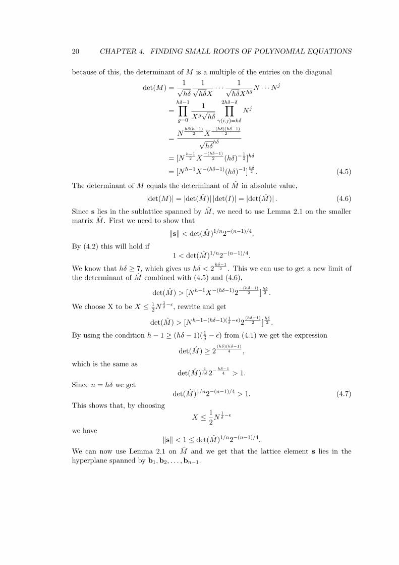
20 CHAPTER 4. FINDING SMALL ROOTS OF POLYNOMIAL EQUATIONS
because of this, the determinant of M is a multiple of the entries on the diagonal
det(M) =1√hδ
1√hδX
· · · 1√hδXhδ
N · · ·N j
=hδ−1∏g=0
1Xg√hδ
2hδ−δ∏γ(i,j)=hδ
N j
=N
hδ(h−1)2 X
−(hδ)(hδ−1)2
√hδ
hδ
= [Nh−1
2 X−(hδ−1)
2 (hδ)−12 ]hδ
= [Nh−1X−(hδ−1)(hδ)−1]hδ2 . (4.5)
The determinant of M equals the determinant of M in absolute value,
|det(M)| = |det(M)| |det(I)| = |det(M)| . (4.6)
Since s lies in the sublattice spanned by M , we need to use Lemma 2.1 on the smallermatrix M . First we need to show that
‖s‖ < det(M)1/n2−(n−1)/4.
By (4.2) this will hold if1 < det(M)1/n2−(n−1)/4.
We know that hδ ≥ 7, which gives us hδ < 2hδ−1
2 . This we can use to get a new limit ofthe determinant of M combined with (4.5) and (4.6),
det(M) > [Nh−1X−(hδ−1)2−(hδ−1)
2 ]hδ2 .
We choose X to be X ≤ 12N
1δ−ε, rewrite and get
det(M) > [Nh−1−(hδ−1)( 1δ−ε)2
(hδ−1)2 ]
hδ2 .
By using the condition h− 1 ≥ (hδ − 1)(1δ − ε) from (4.1) we get the expression
det(M) ≥ 2(hδ)(hδ−1)
4 ,
which is the same asdet(M)
1hδ 2−
hδ−14 > 1.
Since n = hδ we getdet(M)1/n2−(n−1)/4 > 1. (4.7)
This shows that, by choosing
X ≤ 12N
1δ−ε
we have‖s‖ < 1 ≤ det(M)1/n2−(n−1)/4.
We can now use Lemma 2.1 on M and we get that the lattice element s lies in thehyperplane spanned by b1,b2, . . . ,bn−1.

4.1. COPPERSMITH - THE UNIVARIATE CASE 21
4.1.3 Finding the solution x0
We have applied the LLL-algorithm on the rows of the matrix M of size hδ × hδ, andgot a basis b1,b2, . . . ,bn which satisfies (2.1)∥∥∥bn∥∥∥ ≥ det(M)1/n2(n−1)/4,
and together with (4.7) we get ∥∥∥bn∥∥∥ ≥ 1.
From Lemma 2.1 we have that any vector in the lattice generated by the rows of M withlength less than 1 must lie in a hyperplane spanned by b1,b2, . . . ,bn−1.
We can write s as a linear combination of the LLL-reduced basis,
s =hδ∑j=1
ρjbj . (4.8)
But we know that s is a short vector and by Lemma 2.1 we have that
ρhδ = 0.
We can also write s as a linear combination of the rows of M as we did in (4.4) and wecombine this with (4.3),
s =hδ∑i=1
αimi
=hδ∑i=1
αi
hδ∑j=1
hijbj
=hδ∑j=1
bjhδ∑i=1
αihij .
From (4.8) we get that
ρj =hδ∑i=1
αihij ,
and
ρhδ =hδ∑i=1
αihi,hδ = 0.
We know the value of hi,hδ since it is the last column in H−12 .

22 CHAPTER 4. FINDING SMALL ROOTS OF POLYNOMIAL EQUATIONS
We now look at the polynomial vectors r(x) and s(x), they are define as before butnow we have the variable x instead of x0. The r(x) vector is
r(x) =(
1, x, x2, . . . , xhδ−1,−y,−xy, . . . ,−xδ−1y,−y2, xy2, . . . ,−xδ−1yh−1)
which is the same as
r(x) =
(1, x, . . . , xhδ−1,−p(x)
N,−xp(x)
N, . . . ,−xδ−1 p(x)
N,−(p(x)N
)2
, . . . ,−xδ−1
(p(x)N
)h−1).
Let s(x) be the s vector shortened, that is we have removed the zeros in the end and thevariable is x instead of x0,
s(x) =
(1√hδ,
( xX )√hδ,( xX )2√hδ, . . . ,
( xX )hδ−1
√hδ
).
We define a vector of length hδ
σl =
(0, . . . , 0,
( 1X )l−1
√hδ
, 0, . . . , 0
),
where there are zeros except at the (l − 1)th element in the vector. We can write σl asa linear combination of the rows of M , since σl ∈ L(M)
σl =hδ∑i=1
µlimi.
We can now write s(x) as
s(x) =hδ∑l=1
σlxl−1
=hδ∑l=1
xl−1hδ∑i=1
µlimi
=hδ∑i=1
mi
hδ∑l=1
xl−1µli,
where
αi(x) =hδ∑l=1
xl−1µli.

4.2. COPPERSMITH - THE BIVARIATE CASE 23
From before we have that
ρj =hδ∑i=1
αi(x)hij
=hδ∑i=1
(hδ∑l=1
xl−1µli
)hij .
If s(x) is going to be a short vector, then ρhδ must be zero. We get the following equation,
ρhδ =hδ∑i=1
(hδ∑l=1
xl−1µli
)hi,hδ = 0.
We can solve this equation for x, since we know the other variables. We find hi,hδ in thelast column of H−1
2 , µli is in the matrix H−11 . We have the following equation we can
solve for x0,
c(x0) =hδ∑i=1
(hδ∑l=0
xl−10 µli
)hi,hδ = 0.
This equation holds over the integers as well as modulo N and is easy to solve. Thisyields the desired solution x0.
Written in terms of our matrices we can find our new polynomial in this way,
c(x) =[r(x)H−1
1
]sh· ((H−1
2 )hδ)T ,
where [·]sh denote the vector shortened, and ((H−12 )hδ)T is the last column in H−1
2
transposed.
4.2 Coppersmith - the bivariate case
Finding small integer solutions to a polynomial equation in two variables are similar tothe modular case with one variable. The basic outline is the same but this case is moretechnical. We will in the bivariate case get a matrix that is not square, which makes theapproach harder.
We have a polynomial equation in two variables over the integers (not modulo N)with coefficients aij
p(x, y) =δ∑j=0
δ∑i=0
aijxiyj = 0
for which we want to find small integer solutions (x0, y0). The solution is bounded by Xand Y , where x0 < |X| and y0 < |Y |. We assume that p(x, y) has δ as maximum degreein each variable separately and that p(x, y) is irreducible over the integers, which meansthat the coefficients are relatively prime as a set.
24 CHAPTER 4. FINDING SMALL ROOTS OF POLYNOMIAL EQUATIONS
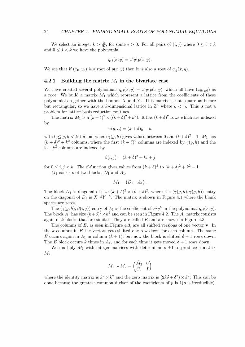
We select an integer k > 23ε , for some ε > 0. For all pairs of (i, j) where 0 ≤ i < k
and 0 ≤ j < k we have the polynomial
qij(x, y) = xiyjp(x, y).
We see that if (x0, y0) is a root of p(x, y) then it is also a root of qij(x, y).
4.2.1 Building the matrix M1 in the bivariate case
We have created several polynomials qij(x, y) = xiyjp(x, y), which all have (x0, y0) asa root. We build a matrix M1 which represent a lattice from the coefficients of thesepolynomials together with the bounds X and Y . This matrix is not square as beforebut rectangular, so we have a k-dimensional lattice in Zn where k < n. This is not aproblem for lattice basis reduction routines.
The matrix M1 is a (k+ δ)2× ((k+ δ)2 + k2). It has (k+ δ)2 rows which are indexedby
γ(g, h) = (k + δ)g + h
with 0 ≤ g, h < k+ δ and where γ(g, h) gives values between 0 and (k+ δ)2− 1. M1 has(k + δ)2 + k2 columns, where the first (k + δ)2 columns are indexed by γ(g, h) and thelast k2 columns are indexed by
β(i, j) = (k + δ)2 + ki+ j
for 0 ≤ i, j < k. The β-function gives values from (k + δ)2 to (k + δ)2 + k2 − 1.M1 consists of two blocks, D1 and A1,
M1 =(D1 A1
).
The block D1 is diagonal of size (k + δ)2 × (k + δ)2, where the (γ(g, h), γ(g, h)) entryon the diagonal of D1 is X−gY −h. The matrix is shown in Figure 4.1 where the blankspaces are zeros.
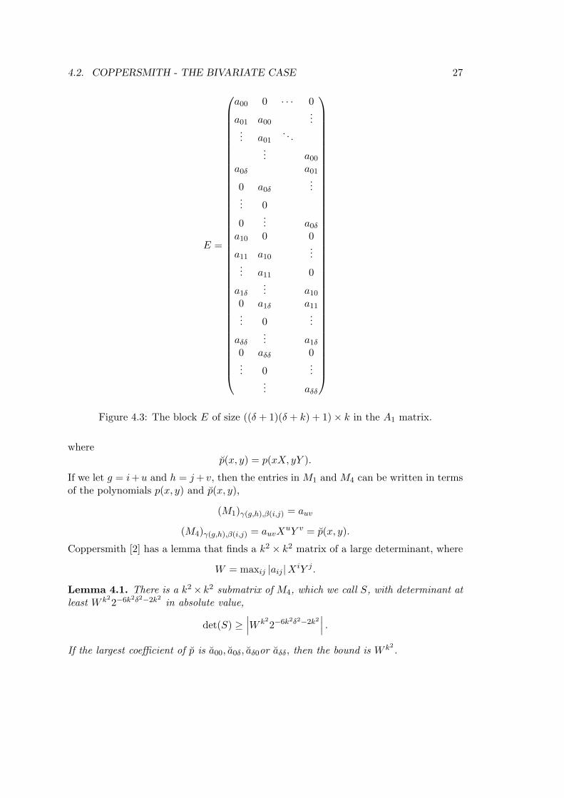
The (γ(g, h), β(i, j)) entry of A1 is the coefficient of xgyh in the polynomial qij(x, y).The block A1 has size (k+δ)2×k2 and can be seen in Figure 4.2. The A1 matrix consistsagain of k blocks that are similar. They are called E and are shown in Figure 4.3.
The columns of E, as seen in Figure 4.3, are all shifted versions of one vector v. Inthe k columns in E the vectors gets shifted one row down for each column. The sameE occurs again in A1 in column (k + 1), but now the block is shifted δ + 1 rows down.The E block occurs k times in A1, and for each time it gets moved δ + 1 rows down.
We multiply M1 with integer matrices with determinants ±1 to produce a matrixM2
M1 ∼M2 =(M2 0C2 I
)where the identity matrix is k2 × k2 and the zero matrix is (2kδ+ δ2)× k2. This can bedone because the greatest common divisor of the coefficients of p is 1(p is irreducible).

4.2. COPPERSMITH - THE BIVARIATE CASE 25
D1 =
1X−0Y −1
X−0Y −2
. . .X−0Y −(k+δ−1)
X−1Y −0
X−1Y −1
. . .X−1Y −(k+δ−1)
X−2Y −0
. . .X−(k+δ−1)Y −(k+δ−1)
Figure 4.1: The diagonal matrix D1.
The top (2kδ + δ2) rows of M2 forms a sublattice of the original lattice and we call thissublattice M2. We do lattice basis reduction on these top (2kδ+ δ2) rows of M2, and wecall the matrix consisting of these new rows M3. We construct a vector r with length(k + δ)2 where the γ(g, h) entry is xg0y
h0 ,
r =(x0
0y00, x
00y
10, . . . , x
00yk+δ−10 , x1
0y00, x
10y
10, x
10y
20, . . . , x
k+δ−10 yk+δ−1
0
).
The row vector s of length (k + δ)2 + k2 is given by s = rM1.
s =((x0
X
)0 (y0
Y
)1, . . . ,
(x0
X
)k+δ−1 (y0
Y
)k+δ−1, q01(x0, y0), . . . , qk−1,k−1(x0, y0)
)Each of the first (k + δ)2 entries are given by
sγ(g,h) =(x0
X
)g (y0
Y
)hand the k2 right-hand side entries are zero,
sβ(i,j) = qij(x0, y0) = 0.
Since x0 < |X| and y0 < |Y | the left-hand side elements satisfies∣∣sγ(g,h)∣∣ < 1
and the length of the vector is‖s‖ < k + δ.
We know that s is generated by the rows of M3 since s has zeros on its right handside. To show that s is a ”relatively short” vector in the lattice, we can confine it to ahyperplane by Lemma 2.1. To be able to do so we need to evaluate the determinant ofthe matrix M1.

26 CHAPTER 4. FINDING SMALL ROOTS OF POLYNOMIAL EQUATIONS
Figure 4.2: The matrix A1 of size (k+ δ)2×k2, where the E block is given in Figure 4.3.
4.2.2 Analysis of the determinant
Let M4 be the matrix obtained from M1 by multiplying the γ(g, h) row by XgY h andmultiplying the β(i, j) column by X−iY −j . M4 can then be written as
M4 = ∆1M1∆2, (4.9)
where ∆1 is a (k+δ)2×(k+δ)2 diagonal matrix and ∆2 is a ((k+δ)2+k2)×((k+δ)2+k2)diagonal matrix. We use the notation diag(·) to express a diagonal matrix where thediagonal elements are listed in the parenthesis. We have
∆1 = diag(
1, Y 1, Y 2, . . . , Y k−δ−1, X1Y 0, X1Y 1, X1Y 2, . . . , X1Y k+δ−1,
X2Y 0, . . . , Xk+δ−1Y k+δ−1)
∆2 = diag(
1, 1, . . . , 1, X0Y 0, X0Y −1, . . . , X0Y −(k−1), X−1Y 0, . . . , X−(k−1)Y −(k−1))
where the number of 1’s in the beginning of ∆2 are (k + δ)2. We get another diagonalmatrix ∆3 of size (k + δ)2 × (k + δ)2 by removing k2 1’s on the diagonal of ∆2.
∆3 = diag(
1, . . . , 1, X0Y 0, X0Y −1, . . . , X0Y −(k−1), X−1Y 0, . . . , X−(k−1)Y −(k−1)).
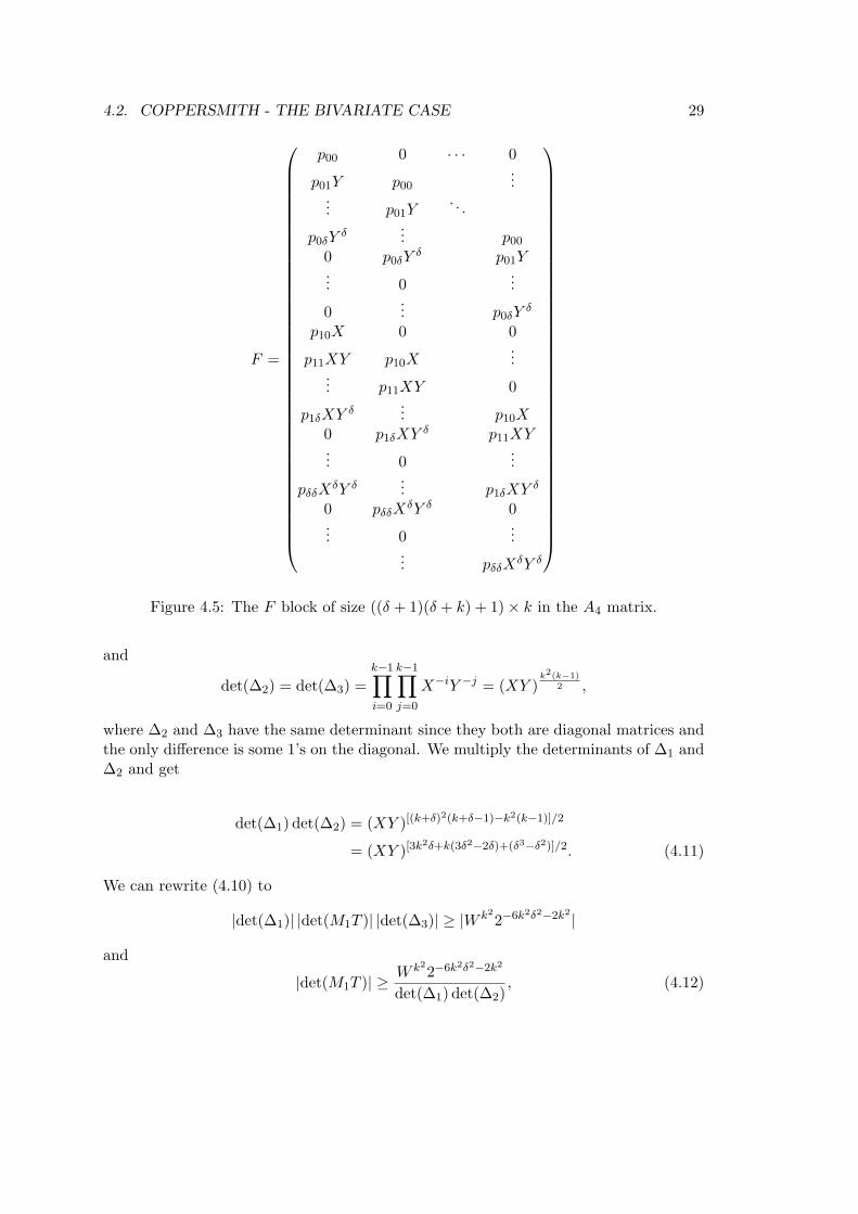
M4 consists of two blocks, the left block is the identity matrix and the right-hand blockis A4 as shown in Figure 4.4 where the blocks are given in Figure 4.5.
M4 =(I A4
)A4 consists again of k blocks, they are identical as seen in Figure 4.5. The blocks are
shifted δ + 1 rows down from the previous block, in the same manner as for the A1
matrix. Each column in block F represents the coefficients of a polynomial
xiyjp(xX, yY ) = xiyj p(x, y)
4.2. COPPERSMITH - THE BIVARIATE CASE 27
E =
a00 0 · · · 0
a01 a00...
... a01. . .
... a00
a0δ a01
0 a0δ...
... 0
0... a0δ
a10 0 0
a11 a10...
... a11 0
a1δ... a10
0 a1δ a11... 0
...
aδδ... a1δ
0 aδδ 0... 0
...... aδδ
Figure 4.3: The block E of size ((δ + 1)(δ + k) + 1)× k in the A1 matrix.
wherep(x, y) = p(xX, yY ).
If we let g = i+u and h = j+ v, then the entries in M1 and M4 can be written in termsof the polynomials p(x, y) and p(x, y),
(M1)γ(g,h),β(i,j) = auv
(M4)γ(g,h),β(i,j) = auvXuY v = p(x, y).
Coppersmith [2] has a lemma that finds a k2 × k2 matrix of a large determinant, where
W = maxij |aij |XiY j .
Lemma 4.1. There is a k2× k2 submatrix of M4, which we call S, with determinant atleast W k2
2−6k2δ2−2k2in absolute value,
det(S) ≥∣∣∣W k2
2−6k2δ2−2k2∣∣∣ .
If the largest coefficient of p is a00, a0δ, aδ0or aδδ, then the bound is W k2.

28 CHAPTER 4. FINDING SMALL ROOTS OF POLYNOMIAL EQUATIONS
Figure 4.4: The matrix A4 of size (k+ δ)2×k2, where the F block is given in Figure 4.5.
Lemma 4.1 finds a k2 × k2 matrix from the right hand block of M4, with largedeterminant. Select 2kδ + δ2 columns of the left hand block of M4 to extend this to a(k+ δ)2× (k+ δ)2 matrix with the same determinant. To make this into a square matrixwe need to fill in with 0’s in the blank spaces. We can rearrange this new matrix andget a matrix with the k2× k2 submatrix of M4 in the upper left corner with 0’s beneathto fill up the rows, and with the columns with 1’s to the right. These can be pickedso that we have an identity block, or at least an invertible block. The determinant ofthis new matrix will be the determinant of the submatrix times the determinant of theinvertible matrix. So the determinant will be greater than or equal to the determinantof the k2 × k2 matrix we have in Lemma 4.1.
Let T be a ((k+δ)2 +k2)×(k+δ)2 permutation matrix which selects the appropriate(k+ δ)2 = (2kδ+ δ2) + k2 columns of M4, so that M4T is a quadratic matrix. From theLemma 4.1 and the discussion above we have
det(M4T ) ≥∣∣∣W k2
2−6k2δ2−2k2∣∣∣
and from (4.9) we get
det(∆1M1∆2T ) ≥∣∣∣W k2
2−6k2δ2−2k2∣∣∣ .
We choose T such that∆2T = T∆3
and getdet(∆1M1T∆3) ≥
∣∣∣W k22−6k2δ2−2k2
∣∣∣ . (4.10)
We compute the determinants of ∆1, ∆2 and ∆3,
det(∆1) =k+δ−1∏h=0
k+δ−1∏g=0
XgY h = (XY )k+δ)2(k+δ−1)
2
4.2. COPPERSMITH - THE BIVARIATE CASE 29
F =
p00 0 · · · 0
p01Y p00...
... p01Y. . .
p0δYδ
... p00
0 p0δYδ p01Y
... 0...
0... p0δY
δ
p10X 0 0
p11XY p10X...
... p11XY 0
p1δXYδ
... p10X0 p1δXY
δ p11XY... 0
...
pδδXδY δ
... p1δXYδ
0 pδδXδY δ 0
... 0...
... pδδXδY δ
Figure 4.5: The F block of size ((δ + 1)(δ + k) + 1)× k in the A4 matrix.
and
det(∆2) = det(∆3) =k−1∏i=0
k−1∏j=0
X−iY −j = (XY )k2(k−1)
2 ,
where ∆2 and ∆3 have the same determinant since they both are diagonal matrices andthe only difference is some 1’s on the diagonal. We multiply the determinants of ∆1 and∆2 and get
det(∆1) det(∆2) = (XY )[(k+δ)2(k+δ−1)−k2(k−1)]/2
= (XY )[3k2δ+k(3δ2−2δ)+(δ3−δ2)]/2. (4.11)
We can rewrite (4.10) to
|det(∆1)| |det(M1T )| |det(∆3)| ≥ |W k22−6k2δ2−2k2 |
and
|det(M1T )| ≥ W k22−6k2δ2−2k2
det(∆1) det(∆2), (4.12)

30 CHAPTER 4. FINDING SMALL ROOTS OF POLYNOMIAL EQUATIONS
where we use that the determinant of ∆2 and ∆3 are the same. We combine (4.11) and(4.12),
|det(M1T )| ≥W k22−6k2δ2−2k2
(XY )−[3k2δ+k(3δ2−2δ)+(δ3−δ2)]/2.
Let this lower bound be called Z.We take M3 as described before, and extend it with the last rows of M2 so that we
get a matrix of size (k + δ)2 × (k + δ)2 + k2. We call this matrix M ′3. We now get M3
as our sublattice.
M1T ∼M ′3T =(M3 0C3 I
).
M ′3T is obtained from M1T by multiplying with integer matrices with determinant 1,so the determinants of the two matrices are the same in absolute value. Since the M3Tmatrix have a block lower triangular structure, we get that the determinant of the M3Tmatrix equals that of M3
|det(M1T )| =∣∣det(M ′3T )
∣∣ =∣∣∣det(M3)
∣∣∣ |det(I)| =∣∣∣det(M3)
∣∣∣ . (4.13)∣∣det(M ′3T )∣∣ = |det(M1T )| ≥ Z. (4.14)
The row sT in M3T is obtained from s by deleting columns and its Euclidean norm isbounded by the length of s,
‖sT‖ ≤ ‖s‖ < k + δ. (4.15)
From (4.13) and (4.14) we get
|det(M3)| = |det(M3T )| ≥ Z. (4.16)
To apply Lemma 2.1 to M3 and sT , with n = 2kδ + δ2 the norm of sT must satisfy
‖sT‖ < det(M3)1n 2−
n−14 .
This requires that (4.15) and (4.16) holds in addition to
k + δ ≤ Z1n 2−
n−14 ,
which translates to(k + δ)n ≤ Z × 2−
n(n−1)4 . (4.17)
We recall that n = 2kδ + δ2 and
Z = W k22−6k2δ2−2k2
(XY )−[3k2δ+k(3δ2−2δ)+(δ3−δ2)]
2 .
After some tedious computations (4.17) can be written as
XY ≤W 2/3δ−ε′214δ/3−o(δ)
where
ε′ ≈ 23k
(1− 2
3δ
).
We now assume that XY satisfies this bound. We use the LLL-algorithm on M3 , andwe can use Lemma 2.1 to confine the short vectors to a hyperplane, included the sTvector.

4.3. HOWGRAVE-GRAHAM - THE UNIVARIATE CASE 31
4.2.3 Finding the solution (x0, y0)
We do this exactly in the same way as in the univariate case. But instead of the s vectorwe now use the sT vector which is shortened. We will need to find more matrices, butwe will in the end get an equation on the same form, but with two variables instead ofone. We denote the equation as
c(x0, y0) =k+δ−1∑g=0
k+δ−1∑h=0
aghxg0yh0 = 0.
All the multiples of p(x, y) of sufficiently low degree are already used to define thesublattice M and c(x, y) is hence not a multiple of p(x, y).
Definition 4.1. Let fa(x) and gc(x) be in Z[x] and let a0, ..., an, c0, ..., cm be elementsin Z. We have two polynomials:
fa(x) = a0 + a1x+ ...+ anxn,
gc(x) = c0 + c1x+ ...+ cmxm.
We define the resultant of fa, gc, res(fa, gc), to be the determinant of this (m+n)×(m+n)matrix
a0 a1 · · · ana0 a1 · · · an
· · ·a0 a1 · · · an
c0 c1 · · · cmc0 c1 · · · cm
· · ·c0 c1 · · · cm
where there are m rows with a and c rows of w. The blank spaces are filled with zeros.
We take the resultant of the polynomials p(x, y) and c(x, y)
q(x) = resy(c(x, y), p(x, y)).
Since p(x, y) is an irreducible polynomial the resultant will give a nonconstant integerpolynomial. Since q(x) only depends on x it is easy to compute its roots, which willinclude x0. Given x0 we can find y’s by solving p(x0, y) = 0, where y0 will then be oneof the roots. We now have the desired solution (x0, y0).
4.3 Howgrave-Graham - the univariate case
An alternative technique for finding small roots of univariate modular equations was putforward by Nicholas Howgrave-Graham in [5]. It is related to Coppersmith’s method,but is more direct. Howgrave-Graham’s method uses polynomials that are multiples of

32 CHAPTER 4. FINDING SMALL ROOTS OF POLYNOMIAL EQUATIONS
p(x) and N , whereas Coppersmith only uses p(x). The matrix in Howgrave-Graham’smethod are smaller than in Coppersmith’s method, and it is lower triangular so it iseasy to find the determinant.
Howgrave-Graham proved that Coppersmith’s algorithm and his algorithm are equiv-alent, but Howgrave-Graham’s may be preferred for computational efficiency.
As for Coppersmith’s method the purpose is to find the small roots of a monic,univariate modular equation
p(x) = a0 + a1x+ a2x2 + · · ·+ aδ−1x
δ−1 + xδ ≡ 0 (mod N).
The solution is x0, and δ is the maximal degree for the polynomial. For any polynomialh(x) and natural number X we have the following upper bound on the absolute size ofh(x)
|h(x)| ≤ |a0|+ |a1x|+ · · ·+ |xδ|≤ |a0|+ |a1X|+ · · ·+ |Xδ|
for all |x| ≤ X.
4.3.1 Building the matrix M5
Howgrave-Graham uses a different indexation, where 1 ≤ i, j ≤ n, v =⌊i−1δ
⌋and
u = i− 1− δv. We define a lower triangular (hδ)× (hδ) matrix M5, where h ≥ 2 and Xa natural number. The matrix M5 = (mij) as seen in Figure 4.6 have entries
mij = eijXj−1,
where eij is the coefficient of xj−1 in
qu,v(x) = N (h−1−v)xu(p(x))v.
We observe that this matrix is smaller than the matrix in Coppersmith’s univariate case.For all u, v ≥ 0 the polynomial equation
qu,v(x0) = 0 (mod Nh−1)
have a solution x0. The determinant of the matrix M5 will be the entries on the diagonal,
det(M5) = Xhδ(hδ−1)N (hδ(h−1))/2. (4.18)
Notice that we can find the determinant directely, and we do not need to find a sublatticeof M5. We can work directely with M5.

4.3. HOWGRAVE-GRAHAM - THE UNIVARIATE CASE 33
M5 =
Nh−1 0 ··· ... 0
0 Nh−1X 0 ···...
.... . . ···
0 ··· 0 Nh−1Xδ−1 0 ···
a0Nh−2 a1Nh−2X ··· Nh−2Xδ 0 ···
0 a0Nh−2X ··· Nh−2Xδ+1
0 0 a0Nh−2X2 ··· Nh−2Xδ+2
.... . .
0 ··· a0Nh−2Xδ−1 a1Nh−2Xδ ··· Nh−2X2δ−1
a20N
h−3 ··· Nh−3X2δ
.... . .
0 0
Figure 4.6: M5 matrix
4.3.2 Finding the solution x0
Let B5 be the LLL-reduced basis of the rows of M5, and the first row vector of B5 is b1.We have that
B5 = H5M5,
for a matrix H5 = B5M−15 . The equation in Proposition 2.2 and (4.18) give
‖b1‖ ≤ 2(hδ−1)/4X(hδ−1)/2N (h−1)/2,
which is exactly the same as in Coppersmith’s case. Let b1 = cM for some c∈Zn. Welook at the norm of b1,
‖b1‖ ≥1√hδ
hδ∑j=1
|b1i|
=1√hδ
(∣∣∣∣∣hδ∑i=1
cimi,1
∣∣∣∣∣+
∣∣∣∣∣hδ∑i=1
cimi,2
∣∣∣∣∣+ · · ·+
∣∣∣∣∣hδ∑i=1
cimi,hδ
∣∣∣∣∣)
=1√hδ
(∣∣∣∣∣hδ∑i=1
ciei,1
∣∣∣∣∣+
∣∣∣∣∣(
hδ∑i=1
ciei,2
)X
∣∣∣∣∣+ · · ·+
∣∣∣∣∣(
hδ∑i=1
ciei,hδ
)Xhδ−1
∣∣∣∣∣)
≥ 1√hδ|h(x)| (4.19)

34 CHAPTER 4. FINDING SMALL ROOTS OF POLYNOMIAL EQUATIONS
for all |x| ≤ X where
h(x) =hδ∑i=1
ciei,1 +
(hδ∑i=1
ciei,2
)x+ · · ·+
(hδ∑i=1
ciei,hδ
)xhδ−1
= c1
hδ∑j=1
e1,jxj−1 + c2
hδ∑j=1
e2,jxj−1 + · · ·+ chδ
hδ∑j=1
ehδ,jxj−1. (4.20)
From (4.19) we observe that b1 is almost an upper bound for the polynomial h(x),for |x| ≤ X. Since each sum in (4.20) is zero modulo Nh−1, we have that
h(x0) ≡ 0 (mod Nh−1).
We combine (4.19) and (4.20) and we can form a polynomial h(x) that satisfies h(x0) ≡ 0(mod Nh−1) and
|h(x)| ≤(
2(hδ−1)
4
√hδ)X
hδ−12 N
h−12
for all |x| ≤ X. Thus choosing
X =⌈(
2−12 (hδ)−
1hδ−1
)N
h−1hδ−1
⌉− 1
shows that we can make a polynomial h(x) such that h(x0) = 0 (mod Nh−1) and |h(x)| <Nh−1 for all |x| ≤ X. This implies that h(x0) = 0 over the integers, for any x0 thatsatisfies |x0| ≤ X and p(x0) = 0 (mod N).
Let us now look at how we can find h(x) by using our matrices. Let the columns ofM5 be mj ,
M5 = (m1 m2 · · · mhδ) .
We create a vector r(x)
r(x) =(
1,x
X,( xX
)2, . . . ,
( xX
)hδ−1).
The polynomial h(x) is created in such a way that
h(x) = h1M5 · r(x)= b1 · r(x),
where h1 is the first row in H5, noticing that b1 = h1M5. As shown above this vectorwill have x0 as a root. We can now solve this univariate polynomial equation overthe integers. After finding the solutions one can test each solution to see if it satisfiesp(x0) ≡ 0 (mod N).

Chapter 5
An example
Given the polynomial
p(x) = x3 − 4x2 − 3x− 10 (mod 1131)
where(p(x))2 = x6 − 8x5 + 10x4 + 89x2 + 60x+ 100.
The degree δ is 3, and we choose h to be 3 so the requirement hδ ≥ 7 is fulfilled. Ouraim is to find the small roots of the polynomial equation,
p(x) = x3 − 4x2 − 3x− 10 (mod 1131) = 0
and we set the requirement X = 6, which means that we will find roots |x0| < 6, if thereexist some. In this small example it is easy to see that x = 5 is a root.
5.1 Coppersmith’s method
We will now try to find the small roots of our polynomial using Coppersmith’s method.We make the matrix as in Coppersmith’s univariate case, and get a 15 × 15 M matrixas shown in Figure 5.1. We take the determinant of the matrix and get
det(M) =153841020405122283630137
203018823308689211155302473269248.
We now want to do row operations on the M matrix, where we can interchange tworows, and multiply one row and add it to another row. After doing about 50 operationswe get the following matrix M on the desirable form, as shown in Figure 5.2. We takethe determinant of this matrix as well and get
det(M) =153841020405122283630137
203018823308689211155302473269248,
and we see that the two determinants are the same as expected. The matrix M is blockupper triangular and we can now look at the smaller matrix M which is a sublattice.
35

36 CHAPTER 5. AN EXAMPLE
19 0 0 0 0 0 0 0 0 −10 0 0 100 0 0
0 154 0 0 0 0 0 0 0 −3 −10 0 60 100 0
0 0 1629
0 0 0 0 0 0 −4 −3 −10 89 60 100
0 0 0 1639
0 0 0 0 0 1 −4 −3 4 89 100
0 0 0 0 1649
0 0 0 0 0 1 −4 10 4 89
0 0 0 0 0 1659
0 0 0 0 0 1 −8 10 4
0 0 0 0 0 0 1669
0 0 0 0 0 1 −8 10
0 0 0 0 0 0 0 1679
0 0 0 0 0 1 −8
0 0 0 0 0 0 0 0 1689
0 0 0 0 0 1
0 0 0 0 0 0 0 0 0 1131 0 0 0 0 0
0 0 0 0 0 0 0 0 0 0 1131 0 0 0 0
0 0 0 0 0 0 0 0 0 0 0 1131 0 0 0
0 0 0 0 0 0 0 0 0 0 0 0 11312 0 0
0 0 0 0 0 0 0 0 0 0 0 0 0 11312 0
0 0 0 0 0 0 0 0 0 0 0 0 0 0 11312
Figure 5.1: The M matrix
We see M in Figure 5.3. We use the LLL-algorithm on this matrix and end up with thematrix B2, as seen in Figure 5.4. The first row is b1, and so on.
We have that M = H1M , and we have computed H−11 as seen in Figure 5.5. After
using the LLL-algorithm on M we get the B2 matrix, and since the LLL-algorithm isjust row operations we can write B2 = H2M . The inverse of the H2 matrix is in Figure5.6.
We have the vector r(x),
r(x) =
(1, x, . . . , xhδ−1,−p(x)
N,−xp(x)
N, . . . ,−xδ−1 p(x)
N,−(p(x)N
)2
, . . . ,−xδ−1
(p(x)N
)h−1)
which in this example is
r(x) =
(1, x, x2, . . . , x8,− p(x)
1131,−x p(x)
1131,−x2 p(x)
1131,−(p(x)1131
)2
, x
(p(x)1131
)2
, x2
(p(x)1131
)2)
where p(x) is our polynomial.

5.1. COPPERSMITH’S METHOD 37
19 0 0 5
9725
145895
34992245
104976815
419904125
78732 0 0 0 0 0 0
0 154 0 1
64811
583297
69984121
1049762447
25194242015
2519424 0 0 0 0 0 0
0 0 1324
1486
1911664
4934992
163139968
305314928
1204715116544 0 0 0 0 0 0
0 0 0 −377648 −377
972 − 716323328 − 377
1296 −214513839808 − 92365
419904 0 0 0 0 0 0
0 0 0 0 − 3773888 − 377
5832 − 414769984 − 4147
69984 − 2755875038848 0 0 0 0 0 0
0 0 0 0 0 − 37723328 − 377
17496 − 37715552 − 10933
419904 0 0 0 0 0 0
0 0 0 0 0 0 −14212946656 −142129
34992 −14212931104 0 0 0 0 0 0
0 0 0 0 0 0 0 −142129279936 −142129
209952 0 0 0 0 0 0
0 0 0 0 0 0 0 0 − 1421291679616 0 0 0 0 0 0
0 0 0 11944
12916
1969984
13888
5692519424
2451259712 1 0 0 0 0 0
0 0 0 0 111664
117496
11209952
11209952
73115116544 0 1 0 0 0 0
0 0 0 0 0 169984
152488
146656
291259712 0 0 1 0 0 0
0 0 0 0 0 0 1419904
1314928
1279936 0 0 0 1 0 0
0 0 0 0 0 0 0 12519424
11889568 0 0 0 0 1 0
0 0 0 0 0 0 0 0 115116544 0 0 0 0 0 1
Figure 5.2: The M matrix.

38 CHAPTER 5. AN EXAMPLE
19 0 0 5
9725
145895
34992245
104976815
419904125
78732
0 154 0 1
64811
583297
69984121
1049762447
25194242015
2519424
0 0 1324
1486
1911664
4934992
163139968
305314928
1204715116544
0 0 0 −377648 −377
972 − 716323328 − 377
1296 −214513839808 − 92365
419904
0 0 0 0 − 3773888 − 377
5832 − 414769984 − 4147
69984 − 2755875038848
0 0 0 0 0 − 37723328 − 377
17496 − 37715552 − 10933
419904
0 0 0 0 0 0 −14212946656 −142129
34992 −14212931104
0 0 0 0 0 0 0 −142129279936 −142129
209952
0 0 0 0 0 0 0 0 − 1421291679616
Figure 5.3: M matrix
We compute r(x)H−11 to get a new polynomial
r(x)H−11 =
(1, x, x2,− p(x)
1131,−x p(x)
1131,−x2 p(x)
1131,−(p(x)1131
)2
, x
(p(x)1131
)2
, x2
(p(x)1131
)2
,
0, 0, 0, 0, 0, 0
).
We now shorten this vector by removing the last 6 entries with zeros. The vector is now9 elements long, so it can be multiplied with the last column of H−1
2 matrix in Figure5.6. We get
[r(x)H−11 ]sh · ((H−1
2 )9)T = − 111312
(p(x))2 = 0.
Finding the roots of this polynomial is the same as finding the roots of p(x), except thatwe do not have a modular equation. We solve and get that x0 = 5 is a root. It is smallerthan the X bound which was 6 in this example, and we got the desired root.
5.2 Howgrave-Graham’s method
We now try to solve the same polynomial equation using Howgrave-Graham’s method.We make the matrix, as seen in Figure 5.7. This matrix is lower triangular, so we do nothave to do all the computations as we did in Coppersmith’s case to get it on this form.
The determinant of the M5 matrix is
det(M5) = 867572859423777011829071392228792942475362723656892416.

5.2. HOWGRAVE-GRAHAM’S METHOD 39
0 0 1324
1486
1911664
4934992
163139968
305314928
1204715116544
0 154 − 1
324 − 11944
13888 − 1
69984 − 5419904
72519424
4315116544
0 0 181
2243
192916 − 739
69984 − 19711664 − 25657
1259712 − 431751889568
0 0 − 1324 − 1
486 − 1911664
103369984
31715552
293171259712 − 224405
3779136
0 0 11324
11486 − 461
5832 − 372187 − 469
139968 − 19157464
232333779136
19 0 − 1
3241
3247
388823
17496491
4199041225
125971211953
15116544
0 0 − 11324 − 11
486 − 20911664
12798748
28367139968 − 695261
2519424 − 42651889568
0 127
41162 − 797
19441573888
31369984 − 1609
1049769311
2519424167177
15116544
0 0 − 127 − 2
81 −12073888
35172592 −160673
13996855063419904 − 87773
5038848
Figure 5.4: The B2 matrix
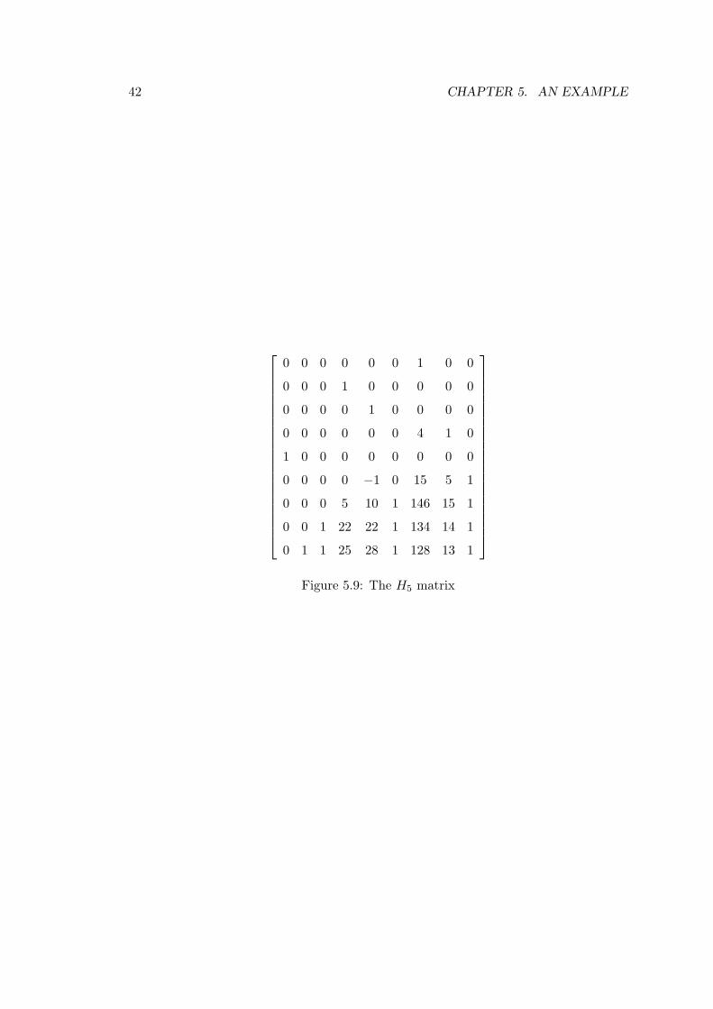
The M5 matrix is LLL-reduced by the LLL-algorithm and we get the B5 matrix, B5 =H5M5. The first row is b1, and so on. The B5 matrix can be seen in Figure 5.8, and theH5 matrix in Figure 5.9.
We now have all the information we need to make the new polynomial which havex0 as a root. We take the dot product of b1 and r(x) which is our constructed vector
r(x) =(
1,x
X,( xX
)2, . . . ,
( xX
)hδ−1).
In this example it will be
r(x) =(
1,x
X,( xX
)2, . . . ,
( xX
)5).
We have that h(x) = b1 · r(x), and we get the following polynomial
h(x) = 100 +3606x+
320462
x2 +86463
x3 +12960
64x4 − 62208
65x5 +
4665666
x6
= 100 + 60x+ 89x2 + 4x3 + 10x4 − 8x5 + x6.
This polynomial have x0 as a root, and we are able to find the roots, one of which isx0 = 5.

40 CHAPTER 5. AN EXAMPLE
1 0 0 0 0 0 0 0 0 −10 0 0 100 0 0
0 1 0 0 0 0 0 0 0 −3 −10 0 60 100 0
0 0 1 0 0 0 0 0 0 −4 −3 −10 89 60 100
0 0 0 0 0 0 0 0 0 1 −4 −3 4 89 100
0 0 0 0 0 0 0 0 0 0 1 −4 10 4 89
0 0 0 0 0 0 0 0 0 0 0 1 −8 10 4
0 0 0 0 0 0 0 0 0 0 0 0 1 −8 10
0 0 0 0 0 0 0 0 0 0 0 0 0 1 −8
0 0 0 0 0 0 0 0 0 0 0 0 0 0 1
0 0 0 1 0 0 0 0 0 1131 0 0 0 0 0
0 0 0 0 1 0 0 0 0 0 1131 0 0 0 0
0 0 0 0 0 1 0 0 0 0 0 1131 0 0 0
0 0 0 0 0 0 1 0 0 0 0 0 1279161 0 0
0 0 0 0 0 0 0 1 0 0 0 0 0 1279161 0
0 0 0 0 0 0 0 0 1 0 0 0 0 0 1279161
Figure 5.5: H−1
1 matrix
1 0 0 0 0 1 0 0 0
1 1 0 0 0 0 0 0 0
1 0 0 0 0 0 0 0 0
−141 −2 6 0 3 0 0 1 0
−19 0 2 0 1 0 0 0 0
−4 0 1 0 0 0 0 0 0
−477 0 145 14 −3 0 4 0 1
−44 0 15 5 0 0 1 0 0
−3 0 1 1 0 0 0 0 0
Figure 5.6: H−1
2 matrix

5.2. HOWGRAVE-GRAHAM’S METHOD 41
1279161 0 0 0 0 0 0 0 0
0 7674966 0 0 0 0 0 0 0
0 0 7674966 0 0 0 0 0 0
−11310 −20358 −162864 244296 0 0 0 0 0
0 −67860 −122148 −162864 244296 0 0 0 0
0 0 407160 −732888 −5863104 8794656 0 0 0
100 360 3204 864 12960 −62208 46656 0 0
0 600 2160 19224 5184 77760 −373248 279936 0
0 0 3600 12960 115344 31104 466560 −2239488 1679616
Figure 5.7: The M5 matrix
100 360 3204 864 12960 −62208 46656 0 0
−11310 −20358 −162864 244296 0 0 0 0 0
0 −67860 −122148 −162864 244296 0 0 0 0
400 2040 14976 22680 57024 −171072 −186624 279936 0
1279161 0 0 0 0 0 0 0 0
1500 76260 184608 284904 91368 −513216 −699840 −839808 1679616
−41950 −718830 −1124856 −712584 −1334880 909792 1679616 1959552 1679616
−235420 −1884156 2275038 1456488 1435968 1578528 1492992 1679616 1679616
−269950 5319816 1032174 1187784 2818800 1874016 1586304 1399680 1679616
Figure 5.8: The B5 matrix
42 CHAPTER 5. AN EXAMPLE
0 0 0 0 0 0 1 0 0
0 0 0 1 0 0 0 0 0
0 0 0 0 1 0 0 0 0
0 0 0 0 0 0 4 1 0
1 0 0 0 0 0 0 0 0
0 0 0 0 −1 0 15 5 1
0 0 0 5 10 1 146 15 1
0 0 1 22 22 1 134 14 1
0 1 1 25 28 1 128 13 1
Figure 5.9: The H5 matrix

Bibliography
[1] Don Coppersmith. Finding a small root of a univariate modular equation. In EU-ROCRYPT, pages 155–165, 1996.
[2] Don Coppersmith. Small solutions to polynomial equations, and low exponent rsavulnerabilities. J. Cryptology, 10(4):233–260, 1997.
[3] Jean-Sebastien Coron. Finding small roots of bivariate integer polynomial equationsrevisited. In Christian Cachin and Jan Camenisch, editors, EUROCRYPT, volume3027 of Lecture Notes in Computer Science, pages 492–505. Springer, 2004.
[4] Jean-Sebastien Coron. Finding small roots of bivariate integer polynomial equations:A direct approach. In Alfred Menezes, editor, CRYPTO, volume 4622 of LectureNotes in Computer Science, pages 379–394. Springer, 2007.
[5] Nick Howgrave-Graham. Finding small roots of univariate modular equations revis-ited. In Michael Darnell, editor, IMA Int. Conf., volume 1355 of Lecture Notes inComputer Science, pages 131–142. Springer, 1997.
[6] A.K Lenstra, H.W Lenstra, and L Lovasz. Factoring polynomials with rationalcoefficients. Matematische Annalen, 261(4), 1982.
43