polynomial roots from companion matrix …...polynomial roots from companion matrix eigenvalues alan...

MATHEMATICS OF COMPUTATIONVOLUME 64, NUMBER 210APRIL 1995, PAGES 763-776

POLYNOMIAL ROOTS FROM COMPANION MATRIX EIGENVALUES

ALAN EDELMAN AND H. MURAKAMI

Abstract. In classical linear algebra, the eigenvalues of a matrix are sometimes

defined as the roots of the characteristic polynomial. An algorithm to compute

the roots of a polynomial by computing the eigenvalues of the corresponding

companion matrix turns the tables on the usual definition. We derive a first-

order error analysis of this algorithm that sheds light on both the underlying

geometry of the problem as well as the numerical error of the algorithm. Our

error analysis expands on work by Van Dooren and Dewilde in that it states

that the algorithm is backward normwise stable in a sense that must be defined

carefully. Regarding the stronger concept of a small componentwise backward

error, our analysis predicts a small such error on a test suite of eight random

polynomials suggested by Toh and Trefethen. However, we construct examples

for which a small componentwise relative backward error is neither predicted

nor obtained in practice. We extend our results to polynomial matrices, where

the result is essentially the same, but the geometry becomes more complicated.

1. Introduction

Computing roots of polynomials may be posed as an eigenvalue problem by

forming the companion matrix. The eigenvalues of this matrix may be found bycomputing the eigenvalues of this nonsymmetric matrix using standard versions

of balancing (very important for accuracy!) [7] followed by the QR algorithm as

may be found in LAPACK or its precursor EISPACK. This is how the MATLABcommand roots performs its computation.

As Cleve Moler has pointed out in [6], this method may not be the bestpossible because

it uses order n2 storage and order «3 time. An algorithmdesigned specifically for polynomial roots might use order n

storage and n2 time. And the roundoff errors introduced corre-

spond to perturbations in the elements of the companion matrix,not the polynomial coefficients.

Moler continues by pointing out that

Received by the editor February 17, 1993 and, in revised form, January 10, 1994.

1991 Mathematics Subject Classification. Primary 65H05, 65F15.Key words and phrases. Algebraic equation, QR method, eigenvalue.

The first author was supported by NSF grant DMS-9120852 and the Applied MathematicalSciences subprogram of the Office of Energy Research, U.S. Department of Energy under ContractDE-AC03-76SF00098.

©199S American Mathematical Society0025-5718/95 $1.00+ $.25 per page

763

License or copyright restrictions may apply to redistribution; see https://www.ams.org/journal-terms-of-use

764 ALAN EDELMAN AND H. MURAKAMI

We don't know of any cases where the computed roots are not

the exact roots of a slightly perturbed polynomial, but such cases

might exist.

This paper investigates whether such cases might exist. Let f¡, i = 1, ... , n ,

denote the roots of p(x) = a0 + axx -\-h an-Xx"~x + xn that are computed

by this method. Further assume that the r¡ are the exact roots of

p(x) = âo + âxx H-h â„-Xxn~l + xn.

What does it mean to say that p is a slight perturbation of p ? We give four

answers, the best one is saved for last. In the definitions, 0(e) is meant to

signify a small though unspecified multiple of machine precision.

1. The "calculus" definition would require that first-order perturbations of

the matrix lead to first-order perturbations of the coefficients.2. A normwise answer that is compatible with standard eigenvalue backward

error analyses is to require that

max|a, -â,-| = 0(e)||C||,

where C denotes the companion matrix corresponding to p, and e denotes

the machine precision.3. A second normwise answer that would be even better is to require that

max \a¡ - a¡\ = 0(e)\\ balance(C)||.

Standard algorithms for eigenvalue computations balance a matrix C by finding

a diagonal matrix T such that B = T~XCT has a smaller norm than C.4. The strongest requirement should be that

\a' ~ ài\ ru \max—¡—p-1 = 0(e).m\

This is what we will mean by a small componentwise perturbation. If a,■■ = 0,

then one often wants ¿, to be 0 too, i.e., ideally one preserves the sparsity

structure of the problem.

It was already shown by Van Dooren and Dewilde [11, p. 576] by a block

Gaussian elimination argument that the calculus definition holds. Their argu-

ment is valid in the more complicated case of polynomial matrices. It imme-diately follows that good normwise answers are available, though it is not clear

what exactly are the constants involved. We found that integrating work by

Arnold [1] with Newton-like identities allows for an illuminating geometrical

derivation of a backward error bound that is precise to first order. Our work

improves on [11] in that we derive the exact first-order perturbation expres-

sion which we test against numerical experiments. Numerical experiments byToh and Trefethen [9] compare this algorithm with the Jenkins-Traub or theMadsen-Reid algorithm. These experiments indicate that all three algorithmshave roughly similar stability properties and further that there appears to be a

close link between the pseudospectra of the balanced companion matrix and the

pseudozero sets of the corresponding polynomial.


POLYNOMIAL ROOTS FROM COMPANION MATRIX EIGENVALUES 765

2. Error analysis

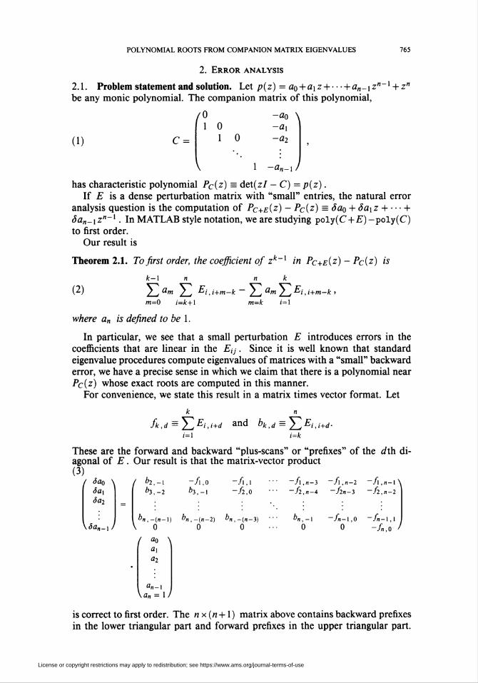
2.1. Problem statement and solution. Let p(z) = ao + axz-\-han-xz"~x + z"

be any monic polynomial. The companion matrix of this polynomial,

(1) C =

1 01 0

V

-flo \

-ax-a2

1 -a„-\J

has characteristic polynomial Pc(z) = det(z/ - C) = p(z).

If E is a dense perturbation matrix with "small" entries, the natural error

analysis question is the computation of Pc+e{z) - Pc(z) — ̂ ao + àaxz -\-h

ôan-Xz"~x. In MATLAB style notation, we are studying poly(C+£')-poly(C)

to first order.Our result is

Theorem 2.1. To first order, the coefficient of zk~x in Pc+e(z) - Pc(z) is

(2)

k—\ n n k

¿__tam ¿_^ Ejj+m-k — y y am y , ■Pf.i+ffi-fc ■

w=0 i=k+l m=k ¡=1

where a„ is defined to be 1.

In particular, we see that a small perturbation E introduces errors in the

coefficients that are linear in the Ey. Since it is well known that standard

eigenvalue procedures compute eigenvalues of matrices with a "small" backward

error, we have a precise sense in which we claim that there is a polynomial near

Pc(z) whose exact roots are computed in this manner.

For convenience, we state this result in a matrix times vector format. Let

fk,d = V, F j t ji = l

and bktd = 'Y^Eij+d.i=k

These are the forward and backward "plus-scans" or "prefixes" of the din di-agonal of E. Our result is that the matrix-vector product

(3)I Sa0 ^ f b2,-\ -f\,o -/i,i

¿3,-1 -/2,05a\Sa2

\San_xJ

bî,-2

bn,-(n-\)

0

( a° \

&2

a„-x\an=\J

—fl,n-3 ~f\,n-2 ~f\,n-\\-f2,n-4 ~/2«-3 ~h,n-2

Qn,-(n-2) -0-3) bn,-\0

"/n-1,0

0-fn-\,\-fn,0

is correct to first order. The nx(n + l) matrix above contains backward prefixes

in the lower triangular part and forward prefixes in the upper triangular part.



The last row of the matrix equation states that perturbing the trace of a matrixperturbs the (negative of the) coefficient of zn~x by the same amount.

If we further assume that the E is the backward error matrix computed by

a standard eigenvalue routine, then we might as well assume that E is nearly

upper triangular. There will also be elements on the subdiagonal, and possibly

on the next lower diagonal, depending on exactly which eigenvalue method is

used.A result analogous to Theorem 2.1 for matrix polynomials may be found in

§4.

2.2. Geometry of tangent spaces and transversality. Figure 1 illustrates matrixspace (Rnxn) with the usual Frobenius inner product

(A, B) = tr(ABT).

The basic players are

p(z) a polynomial (not shown)

C corresponding companion matrixOrb manifold of matrices similar to CTan tangent space to this manifold = [CX - XC : X e Rnxn}

Normal normal space to this manifold= [q(CT) : q is a polynomial}

Syl "Sylvester" family of companion matrices

Normal

: Companion Matrices

C

Figure 1. Matrix space near a companion matrix

• The curved surface represents the orbit of matrices similar to C. These

are all the nonderogatory matrices that have eigenvalues equal to the roots of

p with the same multiplicities. (The dimension of this space turns out to be

n2 -n . An informal argument is that only n parameters are specified, i.e., the

eigenvalues.)• The tangent space to this manifold, familiar to anyone who has studied

elementary Lie algebra (or performed a first-order calculation), is the set of

commutators {CX - XC : X e Rnx"} . (Dimension = n2 - n.)

• It is easy to check that if q is a polynomial, then any matrix of the formq(CT) is perpendicular to every matrix of the form CX - XC. Only slightly



more difficult [1] is to verify that all matrices in the normal space are of the

form q(CT). (Dimension = n.)

• The set of companion matrices (also known as the "Sylvester" family) isobviously an affine space through C. (Dimension = n.)

Proposition 2.1. The Sylvester space of companion matrices is transversal to the

tangent space; i.e., every matrix may be expressed as a linear combination of a

companion matrix and a matrix in the tangent space.

This fact may be found in [1]. When we resolve E into components in these

two directions, the former displays the change in the coefficients (to first order)and the latter does not affect the coefficients (to first order). Actually, a stronger

statement holds: the resolution is unique. In the language of singularity theory,

not only do we have transversality, but also universality : unique + transversal.

We explicitly perform the resolution, and thereby prove the proposition, in the

next subsection.In numerical analysis, there are many examples where perburbations in "non-

physical" directions cause numerical instability. In the companion matrix prob-lem, only perturbations to the polynomial coefficients are relevant to the prob-

lem. Other perturbations are by-products of our numerical method. It is for-

tunate in this case that the error produced by an entire (n2 - n)-dimensionalspace of extraneous directions is absorbed by the tangent space.

2.3. Algebra—the centralizer. Let us take a close look at the centralizer of

C. This is the «-dimensional linear space of polynomials in C, because C

is nonderogatory. Taking the ak as in (1), for k = 0, ... ,n- 1, and lettingan = 1, a¡ = 0 for j £ [0, n], we define matrices

j=k

Clearly, M0 - 0, M„ - I, and the Mk, k = 1, ... , n , span the centralizer ofC.

An interesting relationship (which is closely related to synthetic division) is

that

n

P(t)(t-ciyx = YJMktk-1

k=\

[2, p. 85, equation (32)]. The trace of the above equation is the Newton iden-

tities in generating function form; a variation on the above equation gives the

exact inverse of a Vandermonde matrix [10].

A more important relationship for our purposes is that

Mk = CMk+x+akI, k = 0, 1,2,...,

from which we can inductively prove (the easiest way is backwards from k = n)that



Mk =

( ak

flfe+i

an = 1

\

ak

flfc+i

an = 1

ak

ak+\

an = 1

-Oq

-ax

-ûfc-i

-ao

-Uk-\

)

This is almost the Toeplitz matrix with (/, j) entry equal to ±ak+i_j except

that the left side of the matrix is lower triangular and the right side is strictlyupper triangular.

We are now ready to resolve any E into

(4)E = E*n + EsyX.

All we need is the relationship that expresses how Elitl is perpendicular to the

normal space:

tr(Affc£tan) = 0 for k = 1,..., n.

We therefore conclude from (4) that

(5) Xr(MkE) = \r(MkE*x) = Efn.

Because of the almost Toeplitz nature of the Mk , the trace of MkE involvespartial sums of elements of E along certain diagonals. Writing out this trace,

we have that

k—1 n n k

~*Lk,n = ¿_âm ¿_^ îJ+m-k ~ / „ am / JE¡j+m_k.

m=0 i=k+l m=k i=\

The above expression gives the coefficient of the perturbed characteristic poly-

nomial correct to first order. (Since the coefficients are negated in (1), we are

interested in —Eîn .)

Since £syl is zero in every column other than the last, we may also use (4)

to calculate istan, should we choose. D

3. Numerical experiments

3.1. A pair of 2 x 2 examples. The companion matrices

0 -11 2k and 5 =

01 2

1-3k

for k not too small illustrate many subtleties that occur in floating-point arith-

metic. For convenience, we assume our arithmetic follows the IEEE double-

precision standard, for which k — 27 is large enough to illustrate our point.



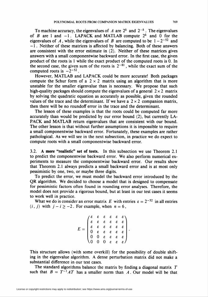
To machine accuracy, the eigenvalues of A are 2k and 2~k . The eigenvalues

of B are 1 and -1. LAPACK and MATLAB compute 2k and 0 for theeigenvalues of A, while the eigenvalues of B are computed to be 1 - 2~52 and-1. Neither of these matrices is affected by balancing. Both of these answersare consistent with the error estimate in (2). Neither of these matrices givesanswers with a small componentwise backward error. In the first case, the given

product of the roots is 1 while the exact product of the computed roots is 0. Inthe second case, the given sum of the roots is 2-81, while the exact sum of the

computed roots is -2~52.

However, MATLAB and LAPACK could be more accurate! Both packages

compute the Schur form of a 2x2 matrix using an algorithm that is more

unstable for the smaller eigenvalue than is necessary. We propose that such

high-quality packages should compute the eigenvalues of a general 2x2 matrix

by solving the quadratic equation as accurately as possible, given the rounded

values of the trace and the determinant. If we have a 2 x 2 companion matrix,

then there will be no roundoff error in the trace and the determinant.

The lesson of these examples is that the roots could be computed far moreaccurately than would be predicted by our error bound (2), but currently LA-

PACK and MATLAB return eigenvalues that are consistent with our bound.

The other lesson is that without further assumptions it is impossible to require

a small componentwise backward error. Fortunately, these examples are rather

pathological. As we will see in the next subsection, in practice we do expect to

compute roots with a small componentwise backward error.

3.2. A more "realistic" set of tests. In this subsection we use Theorem 2.1

to predict the componentwise backward error. We also perform numerical ex-

periments to measure the componentwise backward error. Our results show

that Theorem 2.1 always predicts a small backward error and is at most only

pessimistic by one, two, or maybe three digits.

To predict the error, we must model the backward error introduced by the

QR algorithm. We decided to choose a model that is designed to compensatefor pessimistic factors often found in rounding error analyses. Therefore, the

model does not provide a rigorous bound, but at least in our test cases it seemsto work well in practice.

What we do is consider an error matrix E with entries e = 2-52 in all entries

(i, j) with j - i > -2. For example, when n = 6,

e e\

e ee e

e ee e

e £/

This structure allows (with some overkill) for the possibility of double shift-

ing in the eigenvalue algorithm. A dense perturbation matrix did not make asubstantial difference in our test cases.

The standard algorithms balance the matrix by finding a diagonal matrix T

such that B - T~x AT has a smaller norm than A. Our model will be that

/£ £ £ e

£ £ £ £

£ £ £ £

0 £ £ £0 0 £ £

Vu 0 0 £



the eigenvalue algorithm computes the exact eigenvalues of a matrix B + E',

where \E'\ < E ; i.e., each element of E' has absolute value at most £ above

the second lower diagonal and is 0 otherwise. Therefore, we are computing

the exact eigenvalues of A + TE'T~X. To first order, then, the error in the

coefficients is bounded by the absolute value of the matrix times the absolutevalue of the vector in the product (3), where the scans are computing using

TET~X . This is how we predict the S¡. Further details appear in our MATLABcode in the Appendix.

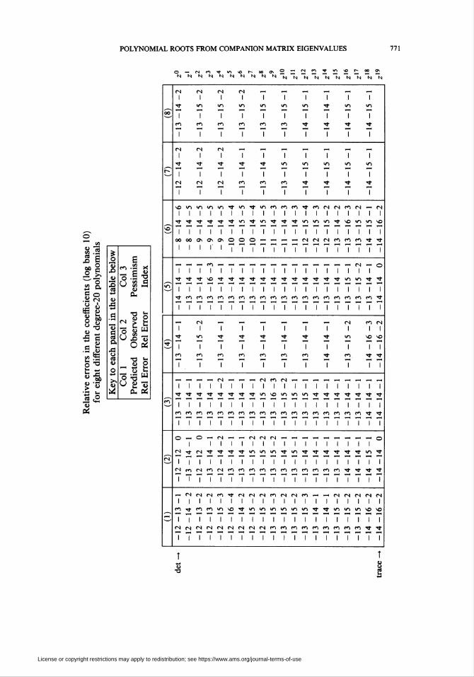
Following [9] exactly, we explore the following degree-20 monic polynomials:

(1) "Wilkinson polynomial": zeros 1, 2, 3, ... , 20,(2) the monic polynomial with zeros equally spaced in the interval [-2.1,

1.9],

(3) />(*) = (20!) E?=0 **/*!.(4) the Bernoulli polynomial of degree 20,(5) the polynomial z20 + z19 + z18 + • ■ • + 1,

(6) the monic polynomial with zeros 2~x0, 2~9, 2~8, ... ,29 ,

(7) the Chebyshev polynomial of degree 20,(8) the monic polynomial with zeros equally spaced on a sine curve, viz.,

(2n/19(k + 0.5)) + isin(2ji/19(ifc + 0.5)), k =-10,-9,-8, ... , 9.

Our experimental results consist of three columns for each polynomial. To

be precise, we first computed the coefficients either exactly or with 30-decimal

precision using Mathematica. We then read these numbers into MATLAB whichmay not have rounded the last bit or two correctly.1 Though we could have

rounded the result correctly in Mathematica, we chose not to do so. Rather, we

took the rounded polynomials stored in MATLAB to be our "official" test cases.Column 1: Log Predicted Error: In the first column we model the predicted

error from (2) in the manner we described above. First we compute the modeledSai, and then display the rounded value of log10 |<fa,/a,|.

Column 2: Log Computed Error: We computed the eigenvalues using MAT-

LAB, and then translated the IEEE double-precision numbers to Mathematica

without any error. We then computed the exact polynomial with these computed

roots and compared the relative backward error in the coefficients.Column 3: Pessimism Index: By taking the ratio of the computed error in

column 2 to the predicted error described in column 1 and then taking the

logarithm and rounding, we obtain a pessimism index. Indices such as 0,-1,

and -2 indicate that we are pessimistic by at most two orders of magnitude;

and index of -19 indicates a pessimism of 19 orders of magnitude. (Since

we are using negative numbers, perhaps we should more properly call this an

optimism index.)There are no entries where the polynomial coefficient is zero. (The Bernoulli

polynomial is a little funny in that it has a z19 term, but no other odd-degree

'Try entering

1.00000000000000018, 1.00000000000000019, and 1.0000000000000001899999999

into MATLAB (fifteen zeros in each number). The results that we obtained on a SUN Sparc Station

10 were 1, 1 + 2~52 , and 1 - 2-52 , respectively, though the correctly rounded result should be

1 + 2~52 in all instances. Cleve Moler has responded that a better string parser is needed.



tq^ts)NNNNNNN NNNNNNNNNN

in

I Ico co

7 7

I Iin in

7 ico m

7 7

in in

Iin in

I Ico m

7 7

i i i

7 7 7

I<N

I Im in in

I I I<N (N <N

7 7 7

i

I

Ico

7

ICO

7

i i i■* ^r ■»

7 7 7*o >n in in in ^frI I I I I I

t » * t t *I I I I I I I I I I I I I

Tj- Su W-) IT! VO

I I I I I I I I I I I I I I I I I I I I

1 ' ' ' '777777777777777

i i i i11 f *

i i i i i i i i i i i

—c fN — O

I I Im »n tí- tj-

I I I I I I I I I I I I I I I I I I I I"^ f*-) ci f^i r*i c*"i co c^ f*1 f} fO f*1 to fi fO fi r*"i fi Cï ^*

77777777777777777777(SI

in

I I I1-

I(N

I I

I ICO CO

7 7 7CO

I

I I

7 7N - h h N n N

I I I I I I II I I I I I I I I I I I I I I I I I I I

I I I I I I I I I I I I I I I I I I I Icocococococococococococococococococo^^

77777777777777777777

I I I I I I I I I<NTtcN^t^'^,,3'>n>ninTt in

I I I I I ITJ- TJ- Tt Tf TT ■* ■n

I I I I I I I I I I I I I I I I I I I I<NcO(NCO<NCOCOCOCOCOCOCOCOCOCOCOtJ-t3.^.^'

iT77777777777777777 i

I I I I I I I I I I I I I I I I I I I Ico^-cocoin^ctTtininininininTj-Ttininin^ovo

I II I I I I I I I I I I I I I I I I INNNriNNNciNmcinnnnpinntt

77777777777777777777



term.) The computed relative error would be infinite in many of these cases.

The top coefficient is the log relative error in the determinant, i.e., the coefficient

of the constant term; the bottom coefficient refers to the trace, i.e., the coefficient

of tX9.

In all cases, we see that the computed backward relative error was excellent.

With the exception of column (6), this is fairly well predicted, usually with

a pessimism index of one to three orders of magnitude. Column (6) is an

exception, where the backward error is far more favorable than we predict.

Why this might be possible was explained in the previous subsection. We

know the determinant to full precision (very rare when performing matrix com-

putations!). So long as our QR shifts and deflation criteria manage not to destroythe determinant, it will remain intact. In column (6) we see a case where this

occurred. By contrast, in the previous subsection we illustrated a case where

this did not occur.We suspect that for any companion matrix, it is often—if not always—

possible to choose shifts and deflation criteria to guarantee high (backward rel-

ative) accuracy even with the smallest of determinants, but we have not proven

this.

4. GENERALIZATION TO MATRIX POLYNOMIALS

A monic matrix polynomial has the form

P(x) = A0 + Axx + ■■■ + An_xx"-X + Ipx" ,

where we assume that the coefficients A¡ (and A„ = Ip) are p x p matrices,

and x is a scalar. It is of interest [3, 4, 5] to find the x for which det(P(x)) =

0 and the corresponding eigenvectors v(x) such that P(x)v(x) = 0. Suchinformation may be obtained from the pn x pn block companion matrix

(6) C =

/0 -Ao \IP 0 -Ax

Ip 0 -A2

Ip -An.xJ

The Sylvester space now has dimension np2, while the tangent space to the

orbit of C generically has dimension n2p2 - np, though it can be smaller.

It seems that if p > 1, we have too many dimensions! We will now show

that we may proceed in a manner that is analogous to that of §2.3 to obtain

what is roughly the same answer, but to do so we must carefully pick a natural

subspace of the tangent space that will give a universal decomposition. This is

not necessary when p - 1. The natural subspace of the tangent space consists

of all matrices of the form CX - XC where the last p rows of X are 0.

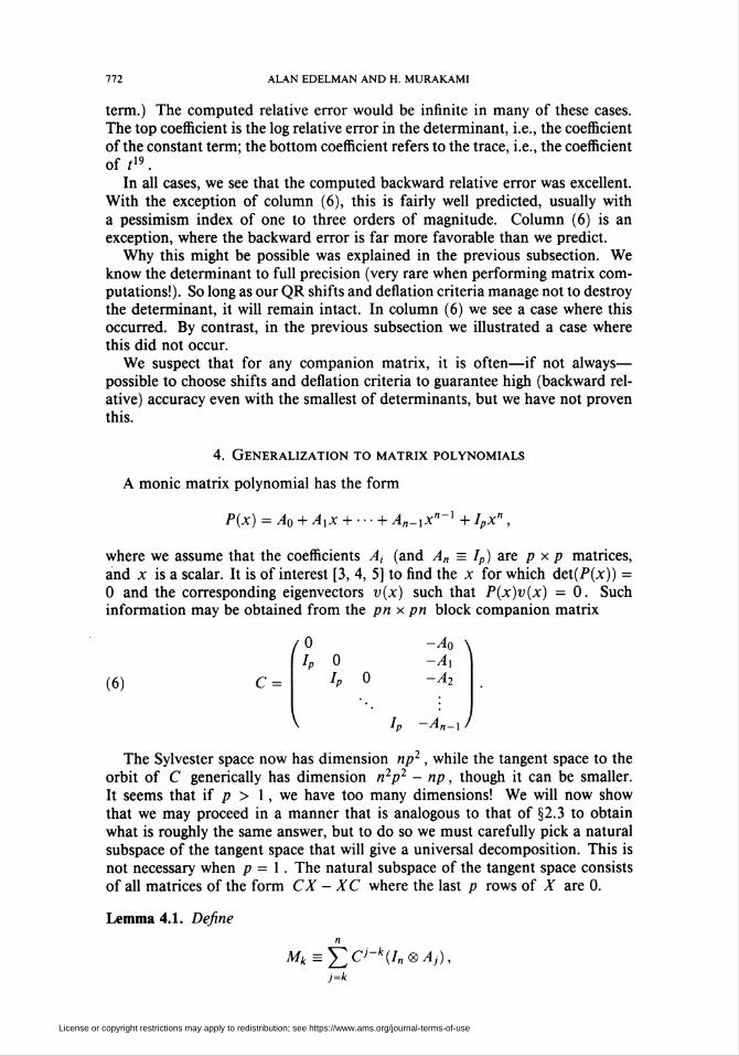
Lemma 4.1. Define

Mk = Y,CJ-k(I„®Aj),

j=k



where <g> denotes the Kronecker product and I„ is the identity matrix of order

n. Then

Mk = CMk+x +In®Ak

and

n-k

( Ak

Ak+X Ak

Ak+X

Mk = An — 'p

An — Ip

V

Ak

Ak+X

An — Ip

-M

-Ax

-Ak-X

-A,

-Ak-\

Proof. These statements are readily verified by induction. D

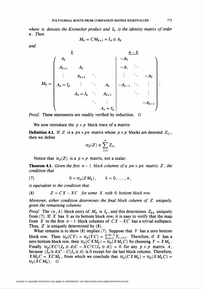
We now introduce the p x p block trace of a matrix:

Definition 4.1. If Z is a pnxpn matrix whose pxp blocks are denoted Z;J,

then we definen

tt>(Z) = £z«.;=1

Notice that trp(Z) is a p x p matrix, not a scalar.

Theorem 4.1. Given the first n - 1 block columns of a pn x pn matrix Z, the

condition that

(7) 0 = \xp(ZMk),

is equivalent to the condition that

k = 0, ... , n,

(8) Z = CX - XC for some X with 0 bottom block row.

Moreover, either condition determines the final block column of Z uniquely,given the remaining columns.

Proof. The (n, k) block entry of Mk is Ip , and this determines Zkn uniquely

from (7). If X has 0 as its bottom block row, it is easy to verify that the map

from X to the first n - 1 block columns of CX - XC has a trivial nullspace.

Thus, Z is uniquely determined by (8).What remains is to show (8) implies (7). Suppose that Y has a zero bottom

block row. Then \rp(CY) = trp(YC) = ¿Z"~x Yiti+X. Therefore, if X has azero bottom block row, then trp(CXMk) = trp(XMkC) by choosing Y = XMk .

Finally Xrp(XC'(In ® A)C - XC'C(In ® A)) = 0 for any p x p matrix A,because (/„ ®A)C- C(I„ ®A) is 0 except for ihe last block column. Therefore,

XMkC = XCMk , from which we conclude that trp(CXMk) = lrp(XMkC) =trp(XCMk). D



We now summarize the geometry.

Corollary 4.1. In the (n2p2)-dimensional space of np xnp matrices, the n2p2-

np2 subspace of the tangent space of the orbit of C defined either by (1) or (8)

is transversal at C to the (np2)-dimensional Sylvester space consisting of block

companion matrices.

We may now resolve any perturbation matrix E into

(9) E = £tan + E*»x,

as in (4), except now EtaD must be in this (n2p2 - np2)-dimensional subspace,

and 2ssyl is 0 except in the final block column. Because trp(ZMk) ^trp(MkZ),

the correct result is that

k-l / n \ n / k \

~Ek\n = ¿Z [ ¿Z EiJ+m-k )Am-¿Z [ ¿ZE'>'+'"-k J Am'm=0 \i=k+\ I m=k \i=\ I

The above expression gives the block coefficient of a perturbed matrix polyno-

mial correct to first order. D

Acknowledgments

We would like to thank Jim Demmel for many interesting discussions and

experiments on transversality and polynomial rootfinding.



Appendix

MATLAB program used in experiments. The numerical part of our experimentswas performed in MATLAB, while the exact component of the experiments

was performed with Mathematica. We reproduce only the main MATLAB code

below for the purpose of specifying precisely the crucial components of our

experiments. The subroutines scan and scanr compute the plus-scan and the

reversed plus-scan of a vector, respectively.

X Predict and compute the componentwise backward error in the eight

X polynomial test cases suggested by Toh and Trefethen.

X - Alan Edelman, October 1993

X Step 1 ... Run Mathematica Program to Compute Coefficients.

X Output «ill be read into matlab as the array

X dl consisting of eight columns and

X 21 rows from the constant term (det) on top

X to the x"19 term (trace), then 1 on the bottom

X (Code not shown.)

X Step 2 ... Form the eight companion matrices

for i-l:8,

•val(['m' num2str(i) '-zeros(20);']);

evaHC'm' num2str(i) '(2:21:380)-ones(l,19) ;']) ;

evaKC'a' num2str(i) '(:,20)=-dl(l:20,* num2str(i), ');']);

end

X Step 3 ... Obtain an "unbalanced" error matrix.

e-eps»ones(20);e=triu(e,-2);

for i»l:8,

eval(['[t,b]-balance(m' num2str(i) ');']);

ti«diag(l./diag(t));

eval(['e' num2str(i) '»(t*e*ti)*norm(b);']);

end

X Step 4 ... Compute the first order perturbation matrix: er.

for j»l:8,

eval(['e=e' num2str(j) ';']);

for»»zeros(20);back=zeros(20);er=zeros(20,21);

for i"l:19

for» * for» + diag(scan(diag(e,i-D) ,i-l) ;

back " back + diag(scanr(diag(e,-i)),-i);

end

er(l:19,l:19)»back(2:20,l:19);er(:,2:21)=er(:,2:21)-forw;

evaHC'er' nua2str(j) '=er;']);

end

X Step 5 ... Compute the predicted relative errors in the coefficients

predicted = zeros(20,8);

for i-l:8,eval(['predicted(:,* num2str(i) ')-abs(er* num2str(i) ')*abs(dl(:,i));']);

end

predicted=abs(predicted./dl(1:20,:));

X Step 6 ... Compute the exact relative errors in the coefficients

X using Mathematica and finally display all relevant

X quantities by taking the base 10 logarithm. (Code not shown.)



BIBLIOGRAPHY

1. V. I. Arnold, On matrices depending on parameters, Russian Math. Surveys 26 (1971),

29-43.

2. F. R. Gantmacher, The theory of matrices, Vols. 1, 2, Chelsea, New York, 1959.

3. I. Gohberg, P. Lancaster, and L. Rodman, Matrix polynomials, Academic Press, New York,

1982.

4. D. Manocha and J. Demmel, Algorithms for intersecting parametric and algebraic curves I:

simple intersections, ACM Trans. Graphics 13 (1994), 73-100.

5. _, Algorithms for intersecting parametric and algebraic curves II: multiple intersections,

Computer graphics, vision and image processing: Graphical models and image processing

(to appear).

6. C. Moler, Cleve's corner: ROOTS—Of polynomials, that is, The MathWorks Newsletter,

vol. 5, no. 1 (Spring 1991), 8-9.

7. B. Parlett and C. Reinsch, Balancing a matrix for calculation of eigenvalues and eigenvectors,

Numer. Math. 13 (1969), 293-304.

8. W. H. Press, B. P. Flannery, S. A. Teukolsky, and W. T. Vetterling, Numerical recipes—The

art of scientific computing, Cambridge Univ. Press, Cambridge, 1986.

9. K..-C. Toh and L. N. Trefethen, Pseudozeros of polynomials and pseudospectra of companion

matrices, Numer. Math. 68 (1994), 403-425.

10. J. F. Traub, Associated polynomials and uniform methods for the solution of linear problems,

SIAM Rev. 8 (1966), 277-301.

11. P. Van Dooren and P. Dewilde, The eigenstructure of an arbitrary polynomial matrix:

computational aspects, Linear Algebra Appl. 50 (1983), 545-579.

Department of Mathematics, Massachusetts Institute of Technology, Cambridge,

Massachusetts 02139E-mail address : edelmanQmath. mit. edu

Quantum Chemistry Laboratory, Department of Chemistry, Hokkaido University,Sapporo 060, Japan

E-mail address : hiroshiQchem2. hokudai .ac.jp


polynomial roots from companion matrix …...polynomial roots from companion matrix eigenvalues alan...

Documents