financial market functioning and monetary policy: japan’s ... · pdf filejapan’s...

39

Financial Market Functioning and Monetary Policy:

Japan’s Experience

Naohiko Baba

This paper reviews the financial market functioning under the zero interestrate policy (ZIRP) and the subsequent quantitative monetary easing policy(QMEP) conducted by the Bank of Japan (BOJ). First, the estimationresults of the Japanese government bond yield curve using the Black-Gorovoi-Linetsky (BGL) model show that (1) the shadow interest rate hasbeen negative since the late 1990s, turned upward in 2003, and has beenon an uptrend since then, and (2) the first-hitting time until the negativeshadow interest rate hits zero again under the risk-neutral probability isestimated to be about three months as of the end of February 2006.Second, under the ZIRP and QMEP, the risk premiums for Japanese bankshave almost disappeared in short-term money markets such as the marketfor negotiable certificates of deposit, while they have remained in the creditdefault swap market and the stock market. This result supports the viewthat market participants have positively perceived the BOJ’s ample liquid-ity provisions in containing the near-term defaults of banks caused by theliquidity shortage.

Keywords: Bank of Japan; Term structure of interest rates; Zero lowerbound; Zero interest rates; Quantitative monetary easing policy; Bank risk premium

JEL Classification: E43, E44, E52, G12

MONETARY AND ECONOMIC STUDIES (SPECIAL EDITION)/DECEMBER 2006

DO NOT REPRINT OR REPRODUCE WITHOUT PERMISSION.

Director and Senior Economist, Institute for Monetary and Economic Studies and FinancialMarkets Department (currently, Financial Markets Department), Bank of Japan (E-mail: [email protected])

Views expressed in this paper are those of the author and do not necessarily reflect the official viewsof the Bank of Japan (BOJ). The author is grateful to Yoichi Ueno for providing insights from aseries of collaborative works, and to other staff including Yuji Sakurai and Mami Sakai of the BOJ for ready assistance. The author also thanks the two designated discussants, David Longworthand Anthony Richards, as well as many conference participants for their invaluable comments and suggestions. Any remaining errors are solely the author’s responsibility.

I. Introduction

This paper aims to review the financial market functioning under the recent mone-tary policy of the Bank of Japan (BOJ): the zero interest rate policy (ZIRP) and thesubsequent quantitative monetary easing policy (QMEP). In doing so, this paperpays particular attention to quantitatively assessing (1) market perceptions about theBOJ’s monetary policy from the Japanese government bond (JGB) yield curve; and(2) the effects of the BOJ’s monetary policy on the risk premiums for Japanese banksin short-term money markets, as well as long-term credit markets such as the creditdefault swap (CDS) and stock markets.

Japan has suffered from an economic slump since the bursting of the bubble economyin the early 1990s. During that time, the Tokyo Stock Price Index (TOPIX) fell byabout 70 percent from its peak to the low in 2003. Declining asset prices severely hit the financial system, the banking sector in particular. Despite the capital injections ofpublic funds into major banks to address the nonperforming-loan (NPL) problem, thebanking sector did not fully recover until quite recently. Business fixed investment con-tinued to suffer from an excess from the late 1980s and the impaired financial system.

In an attempt to find a breakthrough, the BOJ responded with (1) a lowering ofthe uncollateralized overnight call rate to 0.5 percent after the end of 1995, (2) a further lowering to almost zero percent after February 1999 (ZIRP), and (3) theadoption of the quantitative monetary easing policy (QMEP) after March 2001. As argued in Baba et al. (2005) and Ueda (2005), the ZIRP and QMEP have been anattempt to influence expectations about future monetary policy, rather than to changetoday’s policy instrument. In this sense, the ZIRP and QMEP are often called an exercise in expectations management or in shaping expectations.

The QMEP had two pillars: (1) provision of ample liquidity with the outstandingbalance of current accounts at the BOJ as its operating policy target; and (2) “a commitment” to maintain the policy until the year-on-year rate of change in the core consumer price index (CPI)—the core CPI inflation rate—registers zero percentor higher on a sustainable basis.1 To that end, the BOJ has actively used various typesof market operations including a purchasing operation for long-term JGBs. Thus, itseems fair to say that the QMEP augmented the ZIRP in terms of both easing effectsand expectations management.

Japan’s economy finally started recovering in January 2002, and the core CPIinflation rate rose to zero in October 2005, and turned positive the following month.Reacting to these circumstances, the BOJ ended the QMEP in March 2006 andreturned to the ZIRP.2

Given the above nature of the ZIRP and QMEP, some authors have tried to esti-mate the effects of the BOJ’s attempt to manage expectations on the JGB yield curve.They share a common framework: a macro-finance approach. Bernanke, Reinhart, and Sack (2004) and Oda and Ueda (2005) are such examples. Under the macro-finance

40 MONETARY AND ECONOMIC STUDIES (SPECIAL EDITION)/DECEMBER 2006

1. The core CPI means the CPI excluding fresh food. 2. The official statement released by the BOJ after the Monetary Policy Meeting on March 9, 2006 was as follows:

“[T]he Bank of Japan decided to change the operating target of money market operations from the outstanding balance of current accounts at the Bank to the uncollateralized overnight call rate . . . The Bank of Japan willencourage the uncollateralized overnight call rate to remain at effectively zero percent.”

framework, they add a specific macroeconomic structure to the JGB yield curve model.This framework is useful in directly analyzing how some specific macro-factors influ-ence the entire or part of the JGB yield curve. On the other hand, they rely exclusivelyon the specific macroeconomic structure they choose, which leaves an ad hoc inkling.In addition, their models do not seem to closely trace the actual JGB yield curve.3

This paper attempts to review the effects of the BOJ’s expectations management onthe JGB yield curve using a totally different approach from the macro-financeapproach: the Black model of interest rates as options. Black (1995) interprets a nom-inal short-term interest rate as a call option on the “equilibrium” or “shadow” interestrate, where the option is struck at zero percent. Put differently, Black (1995) arguesthat the nominal short-term interest rate cannot be negative since currency serves as anoption, in that if an instrument should have a negative interest rate, investors choosecurrency instead. Employing this notion enables us to use an underlying (shadow) spotrate process that can take on negative values and simply replace all the negative valuesof the shadow interest rate with zeros for the observed short-term nominal interest rate.

The Black model has the following advantages over other types of models such asa macro-finance model. First, we do not need to assume any ad hoc macroeconomicstructure. Second, we can significantly improve the fitting to the actual JGB yieldcurve. Third, we can directly incorporate the notion of “a zero lower bound on theshort-term nominal interest rate” in a more straightforward manner. Fourth, we can directly assess the time period until the negative shadow interest rate first hitszero as the expected duration of the ZIRP, as well as the market expectations aboutthe long-run level of the shadow interest rate.4,5

While the basic concept of the Black model is quite robust and is appealing particularly to the recent Japanese situation where short-term interest rates haveindeed been zero, the model had the disadvantage in that it was analyticallyintractable.6 Quite recently, however, Gorovoi and Linetsky (2004) successfully derivethe analytical solutions for zero-coupon bonds using eigenfunction expansions underseveral specifications for the shadow interest rate process. We follow their solutions,and thus we call the model the Black-Gorovoi-Linetsky (BGL) model in this paper.

Another important task of the BOJ’s monetary policy during the QMEP periodwas to alleviate concerns over the financial-sector problems. As described in Baba et al.(2005), many of the BOJ’s market operations had the dual role of providing ample liquidity and addressing problems in the financial sector. In the process, the BOJassumed a certain amount of credit risk. This paper also assesses the market percep-tions about this aspect of the BOJ’s policy by observing the price developments in various markets, from short-term money markets to the CDS and stock markets.The main objective here is to investigate the time horizons over which the effect of

41

Financial Market Functioning and Monetary Policy: Japan’s Experience

3. For instance, Bernanke, Reinhart, and Sack (2004) find that the predicted JGB yield curves lie above the actualyield curves after 1999 and the deviation narrows in November 2000 after the end of the ZIRP, and widens againin June 2001 with the adoption of the QMEP. This result implies that their macro-finance model does not closelytrace the actual JGB yield curves.

4. Further, we do not even need to assume specific distributions for the timing of the policy change. 5. Black (1995) originally recommends applying his model to the U.S. situation in the 1930s, which was also a

period of extremely low interest rates. On the other hand, Gorovoi and Linetsky (2004) and Baz, Prieul, andToscani (1998) strongly recommend applying the Black model to the recent Japanese situation.

6. See Rogers (1995, 1996) for this line of criticism.

the BOJ’s monetary policy extended in calming market perceptions about the creditrisk for the Japanese banks.

The rest of the paper is organized as follows. Section II presents an overview of theprice developments in the Japanese financial markets under recent monetary easingpolicy conducted by the BOJ. Section III reviews the effects of the BOJ’s monetarypolicy on the JGB yield curve, paying particular attention to the market perceptionsabout the BOJ’s monetary policy stance. Section IV investigates the influences of theBOJ’s monetary policy on the risk premiums for Japanese banks in short-term moneymarkets, as well as the CDS and stock markets. Section V concludes the paper by discussing the policy implications of the findings.

II. Recent Price Developments in the Japanese FinancialMarkets

A. The BOJ’s Monetary Policy and the Interest Rate EnvironmentFirst, let me summarize monetary policy actions by the BOJ since the 1990s. The BOJ started to ease in 1991, then lowered the uncollateralized overnight call rate to 0.5 percent in 1995. This, however, was not enough to counteract deflationary pressures. The BOJ further lowered it to 0.25 percent in 1998, and to effectively zeropercent in February 1999, which is the start of the ZIRP. In April 1999, the BOJpromised to maintain the zero interest rates until “the deflationary concerns are dispelled.” Then, Japan’s economy recovered, growing at 3.3 percent between the thirdquarter of 1999 and the third quarter of 2000. Consequently, the BOJ abandoned theZIRP in August 2000. Japan’s economy, however, went into a serious recession again,together with other advanced economies, led by worldwide declines in the demand for high-tech goods as an aftermath of the bursting of the “IT bubble.”

To cope with the deflationary pressures, the BOJ introduced the QMEP in March2001. The QMEP consisted of (1) supplying ample liquidity using the currentaccount balances (CABs) held by financial institutions at the BOJ as the operatingpolicy target, and (2) the commitment to maintain ample liquidity provision untilthe core CPI inflation rate became zero or positive on a sustainable basis. The targetfor the CABs was raised several times, reaching ¥30–35 trillion in January 2004,which amounts to more than five times the required reserves. Consequently, theactual CABs rose substantially under the QMEP, as shown in Figure 1. To meet thetarget, the BOJ conducted various purchasing operations for instruments such as billsand CP, in addition to treasury bills (TBs) and long-term JGBs.7

The uncollateralized overnight call rate declined to 0.01 percent under the ZIRP,and declined further to 0.001 percent under the QMEP. Medium- and long-terminterest rates also declined substantially, as shown in Figure 2. Interest rates in Japanhave also been quite low in comparison with other countries such as the United States


7. The two building blocks of the QMEP, (1) ample liquidity provision and (2) the commitment to maintain ample liquidity provision, as well as (3) the use of various types of market operations, purchasing of long-term JGBs, in particular, roughly correspond to the three policy prescriptions for stimulating the economy without lowering current interest rates, proposed by Bernanke and Reinhart (2004).

43


Figure 1 Current Account Balances under the QMEP

0

10

20

30

40¥ trillions

Mar.2001

Mar.02

Mar.03

Mar.04

Mar.05

Current account balances (CABs)Required reserves

Source: Bank of Japan.

Figure 2 Interest Rate Environment in Japan

0.0

0.5

1.0

1.5

2.0

2.5

3.0

3.5

4.0

4.5

5.0Percent

ZIRP QMEP

Jan.1995

Jan.96

Jan.97

Jan.98

Jan.99

Jan.2000

Jan.01

Jan.02

Jan.03

Jan.04

Jan.05

Jan.06

Five years10 years20 yearsCall rate (overnight)

Note: Five-, 10-, and 20-year interest rates are the zero-coupon JGB yields estimatedfrom the prices of coupon bonds using McCulloch’s (1971) method. The call rateis the uncollateralized overnight call rate.

Sources: Japan Securities Dealers Association, Bank of Japan.


Figure 3 International Comparison of 10-Year Interest Rates

0

1

2

3

4

5

6

7

8

9

Jan.1995

Jan.96

Jan.97

Jan.98

Jan.99

Jan.2000

Jan.01

Jan.02

Jan.03

Jan.04

Jan.05

Jan.06

JapanUnited StatesGermany

Percent

Note: Interest rates are 10-year yields on government bonds in each country.

Source: Bloomberg.

8. As shown in Baba et al. (2005), long-term JGB yields in recent years are also lower than long-term U.S. governmentbond yields in the 1930s.

9. TIBOR and LIBOR are the Tokyo Interbank Offered Rate and London Interbank Offered Rate, respectively. For more details on them, see Baba and Nishioka (2005) and Ito and Harada (2004).

10. The following financial institutions failed in 1997: Sanyo Securities (November 3), Hokkaido Takushoku Bank(November 17), Yamaichi Securities (November 24), and Tokuyo City Bank (November 26). The concern overthe financial stability continued until Long-Term Credit Bank of Japan (October 23, 1998) and Nippon CreditBank (December 12, 1998) were nationalized.

and Germany, as shown in Figure 3.8 The BOJ ended the QMEP on March 9, 2006,and returned to the ZIRP.

B. Interest Rates in Short-Term Money MarketsNext, let me look at the interest rates in short-term money markets. First, credit risks of Japanese and non-Japanese banks are expected to be priced in TIBOR andLIBOR, since the majority of referenced banks for TIBOR and LIBOR are Japaneseand non-Japanese banks, respectively.9 Indeed, the so-called “Japan premium,” gener-ally defined as the spread between TIBOR and LIBOR (the TL spread), rose sharplyto nearly 100 basis points in U.S. dollars and 40 basis points in yen at the height of the Japanese financial crisis in 1997–98.10 The Japan premium was also considered to reflect non-Japanese major banks’ skepticism concerning the opaque Japaneseaccounting and banking supervision system beyond a simple relative indicator of creditrisk, as suggested by Ito and Harada (2004). As shown in Figure 4, the TL spread hasfluctuated around zero since the adoption of the ZIRP in 1999. Another noteworthypoint here is as follows. Around 2001 to 2002, concerns over the instability of Japanesebanks became highlighted again, mainly due to their low earnings and newly emergingNPLs. This time, however, the TL spread did not widen at all. Ito and Harada (2004)

assert that the TL spread lost its role as an indicator of the market perceptions aboutthe vulnerability of Japanese banks.

Another important indicator of credit risks for Japanese banks is the interest rateson negotiable certificates of deposit (NCDs). NCDs are debt instruments issued bybanks, including city, regional, trust, and foreign banks in Japan. They were the first-ever product with deregulated interest rates in Japan and, since they are uninsured bydeposit insurance, NCD interest rates are expected to reflect credit risks for issuingbanks.11 Figure 5 plots the spread of the NCD interest rate over the BOJ’s target levelof the uncollateralized overnight call rate, together with the TIBOR spread over thesame target call rate. Note here that since the adoption of the QMEP, both NCD andTIBOR spreads have remained stable at a very low level with only one temporaryspike toward the end of fiscal 2001, despite the reemergence of financial instabilityaround 2001 and 2002.

C. Longer-Term Credit SpreadsThird, let me turn to the long-term credit spreads. As shown in Figure 6, credit spreadsof corporate bonds over the JGB yields with the same maturity narrowed following the adoption of the ZIRP. From this figure, we can observe two significant surges in the credit spreads, particularly on BBB-rated bonds. The first surge was from the endof 1997 to 1999, as in the TL and NCD spreads (Figures 4 and 5). The second surge occurred around 2002. This period also corresponds to the period of financial

45


Figure 4 TIBOR/LIBOR and the TL Spread

Percent

ZIRP QMEP

–0.4

–0.2

0.0

0.2

0.4

0.6

0.8

1.0

1.2

1.4

Mar.1996

Mar.97

Mar.98

Mar.99

Mar.2000

Mar.01

Mar.02

Mar.03

Mar.04

Mar.05

Mar.06

TIBOR (three-month)LIBOR (three-month)TL spread

Note: TIBOR and LIBOR in this figure are denominated in euroyen.

Source: Bloomberg.

11. See Baba et al. (2006) for more details about the NCD market in Japan.


Figure 5 NCDs and TIBOR Spread over the Target Call Rate

Percent

ZIRP QMEP

0.0

0.2

0.4

0.6

0.8

Feb.1996

Feb.97

Feb.98

Feb.99

Feb.2000

Feb.01

Feb.02

Feb.03

Feb.04

Feb.05

Feb.06

NCDs (three-month)TIBOR (three-month)

Note: Spreads are calculated as NCD interest rate/yen-TIBOR minus the target uncollateralized overnight call rate.

Source: Bloomberg.

Figure 6 Credit Spreads of Corporate Bonds

Percent

ZIRP QMEP

0.0

0.5

1.0

1.5

Dec.1997

Dec.98

Dec.99

Dec.2000

Dec.01

Dec.02

Dec.03

Dec.04

Dec.05

AAABBB

Note: The spread is defined as the five-year corporate bond interest rate minus theJGB yield with the same maturity. Credit rating is that of Moody’s.

Source: Japan Securities Dealers Association.

47


instability, as mentioned above.12 Since around 2003, credit spreads have substantiallynarrowed and the narrowing has extended even to corporate bonds with a BBB creditrating. Baba et al. (2005) show that credit spreads have barely covered ex post defaultrisks for such bonds with relatively lower ratings. Despite such favorable conditions for issuers, the issue amounts of corporate bonds have not increased much.

Wrapping up the developments in short-term money markets, JGB markets, and corporate bond markets, the following observation can be made, as argued byBaba et al. (2005). Declines in short-term interest rates forced Japanese investors tolook for higher yields by taking various risks in other markets. They first turned toduration risk by investing their funds in longer-term JGBs. Following the decline inlong-term JGB yields, however, they began to expect large potential capital losses inthe event of a reversal of interest rates. Facing such circumstances, Japanese investorsnext turned to credit instruments such as corporate bonds. Their active investmentsin these instruments have substantially narrowed credit spreads even for bonds withrelatively low ratings.13

D. Stock PricesFourth, Figure 7 shows stock price indices: the TOPIX and the stock price index of the banking sector. Both indices have exhibited very similar movement since 1995,

12. In addition, MYCAL Corporation filed for bankruptcy protection in September 2002, which worsened the sentiments of the overall credit markets.

13. This investment behavior is sometimes called “reaching for yield,” investing in assets with returns too low to be justified by rational economic agents. Nishioka and Baba (2004) support the existence of this type of activity by investigating the pricing in the Japanese government and corporate bond markets using the three-factor capital asset pricing model, where mean, variance, and skewness of returns are evaluated in determining the optimal portfolio.

Figure 7 Stock Prices

Percent

Jan.1995

Jan.96

Jan.97

Jan.98

Jan.99

Jan.2000

Jan.01

Jan.02

Jan.03

Jan.04

Jan.05

Jan.06

0.0

0.2

0.4

0.6

0.8

1.0

1.2

Banking sectorTOPIX

Note: The stock price index of the banking sector and the TOPIX are both normalized at January 4, 1995 = 1.

Source: Bloomberg.

but the bank index experienced much more severe slumps during the financial crisisof the late 1990s and the period of financial instability around 2001 to 2002. Thesimilar movement is due mainly to the large capitalization share of bank stocks in theTOPIX, but we should not overlook the fact that a large decline in stock prices itselftriggered the financial instability seen in September 2001, particularly when theTOPIX declined below the 1,000 mark. Not surprisingly, the stock prices of bankswith large stockholdings fell substantially in this period. Then, as the disposal ofNPLs gradually progressed, the stock prices of banks started to recover from the start of 2003. The TOPIX has returned to almost the same level in January 2006 as in January 1995, but the bank index remains at about 60 percent of the value as ofJanuary 1995.14

III. The BOJ’s Monetary Policy and the JGB Yield Curve

A. JGB Yield CurveThis section reviews the effects of the BOJ’s monetary policy on the JGB yield curve,giving particular attention to quantitatively assessing the JGB market perceptions aboutthe BOJ’s monetary policy. First, Figure 8 displays the transition of the JGB yield curvesince the start of the ZIRP in February 1999. Evidently, the flattening of the JGB yield


14. Ito and Harada (2006) provide a detailed survey of the developments in bank stock prices from the late 1990s.

Figure 8 Transition of the JGB Yield Curve

0.0

0.5

1.0

1.5

2.0

2.5

3.0

3.5

0 5 10 15 20

Percent

Time to maturity (years)

Feb. 12, 1999Aug. 11, 2000Mar. 19, 2001June 10, 2003Feb. 28, 2006

Note: Each date corresponds to the following: • February 12, 1999: start of the ZIRP.• August 11, 2000: end of the ZIRP.• March, 19, 2001: start of the QMEP.• June 10, 2003: peak of the QMEP.• February 28, 2006: almost at the end of the QMEP (end of sample period).

Source: Japan Securities Dealers Association.

curve, together with an overall downward shift, sufficiently progressed under the ZIRPand QMEP until the middle of 2003. As a result, conventional yield curve models such as the Vasicek or the Cox, Ingersoll, and Ross (CIR) models no longer successfullytrace the changing shape of the JGB yield curve.15 Extremely low levels of short- andmedium-term interest rates reflect the market participants’ perceptions about the duration of the ZIRP, which was explicitly committed to by the BOJ to maintain thecore CPI inflation rate as a policy guideline by the BOJ under the QMEP. In fact, the thrust of the ZIRP and QMEP lies in “managing expectations,” as argued by Babaet al. (2005) and Ueda (2005). In what follows, let me review the estimation resultsfrom applying the Black model of interest rates as options to the JGB yield curve. The model turned out to be very useful in fitting to the extremely flattened JGB yield curve and quantitatively assessing the duration of the ZIRP expected by the JGBmarket without adding any ad hoc macroeconomic structure to the model.

B. The Black Model of Interest Rates as OptionsBlack (1995) assumes that there is a shadow instantaneous interest rate that can becomenegative, while the observed nominal interest rate is a positive part of the shadow interest rate. The rationale for this assumption is quite straightforward. As long asinvestors can hold currency with zero interest rates, nominal interest rates on otherfinancial instruments must remain non-negative to rule out arbitrage. Specifically, the observed nominal interest rate rt can be written as

rt = max[0, rt*] = rt

* + max[0, −rt*], r0

* = r, (1)

where rt* is the shadow interest rate. The relationship between rt and rt

* is illustrated in Figure 9. In other words, equation (1) shows that the observed nominal interestrate can be viewed as a call option on the shadow interest rate that is struck at zeropercent. Also, the second equality in equation (1) tells us that the observed nominalinterest rate can be expressed as the sum of the shadow interest rate and an option-like value that provides a lower bound for the nominal interest rate at zero percentwhen the shadow interest rate is negative. Let me call this option-like value the floorvalue in this paper, following Bomfim (2003). In other words, the floor has theoption to switch investors’ bondholdings into currency, if rt

* falls below zero. Under normal circumstances, rt

* is sufficiently above zero so that the floor value inequation (1) can be safely ignored. When short-term nominal interest rates are atzero or near zero, however, long-term interest rates embed more-than-usual term premiums and thus the expectations about the future movements of short-term interest rates.

The slope of the term structure for time to maturity T can be written by

1R (r,T ) − r0 = ––– ∫T

s =0f (r, s )ds − max[0, r ], (2)

T

49


15. See Vasicek (1977) for the Vasicek model, and Cox, Ingersoll, and Ross (1985) for the CIR model.

where R (r, T ) − r0 can thus be interpreted as the value of a portfolio of options since R (r, T ), the yield to maturity, is an average of instantaneous forward rates,f (r, s ) (s = 0, . . . , T ), and each of the forward rates exhibits option properties. Morespecifically, f (r, s ) can be viewed as

f (r, s ) = Er[rs ] + forward premium + floor value, (3)

where Er[•] ≡ E [•r0* = r ]. As discount bond prices are derived from forward rates, the

floor value is compounded all over the yield curve, resulting in a steeper yield curvethan the curve that could be expected should currency not exist.

How should we interpret the shadow interest rate in the Black model? Let me firstpresent the view of Black (1995) himself.16 Suppose a situation where the equilibriumnominal interest rate that clears the savings-investment gap is negative. Figure 10illustrates such a situation for a given rate of expected inflation. This situation is akinto the so-called liquidity trap, where under deflationary pressures very low nominalinterest rates cause people to hoard currency. As a result, it neutralizes monetary policy attempts to restore full employment.17 In Figure 10, savings and investment, or supply and demand of capital, are equal at a negative value of r *. The prevailinginterest rate is zero, however, since currency exists. This leaves the savings-investmentgap uncleared. Real-life examples of such situations include the United States duringthe Great Depression in the 1930s (Black [1995] and Bernanke [2002]), and Japansince the 1990s (Krugman [1998]).

The second interpretation is that the shadow interest rate may give us a clue to the length of time until the short-term interest rate becomes positive again, given that


Figure 9 Shadow and Nominal Interest Rates

–5

–4

–3

–2

–1

0

1

2

3

4

Percent

Percent

5

–5 –4 –3 –2 –1 10 2 3 4 5

Shadow interest rate r *

Nominal interest rate rFloor value

16. Bomfim (2003) and Baz, Prieul, and Toscani (1998) follow this interpretation.17. See Keynes (1936), Hicks (1937), and Robertson (1948) for classical debates about the liquidity trap. For Japan’s

recent case, see Krugman (1998) and Baz, Prieul, and Toscani (1998).

the current shadow interest rate is negative. In this sense, the expected time for the negative shadow interest rate to become positive again (the first-hitting time) isregarded roughly as the duration of the ZIRP perceived by the JGB market participants.Note here that if the JGB market participants think that the BOJ will continue theZIRP until Japan’s economy breaks out firmly from the liquidity trap, both inter-pretations coincide with each other. Considering the BOJ’s official statement “untildeflationary concerns are dispelled” and the BOJ’s cautiousness in setting monetarypolicy, the JGB market participants are likely to think in this manner.

On the other hand, the Black model of interest rates as options had a disadvantagein that it was analytically intractable. In fact, Rogers (1995, 1996) criticizes the Black model for this reason and favors models with a reflecting boundary at the zerointerest rate, despite the criticism on economic grounds.18 Gorovoi and Linetsky(2004), however, show that the Black model is as analytically tractable as the reflectingboundary models, and successfully obtain analytical solutions for zero-coupon bondsunder several specifications for the shadow interest rate process. In addition, Linetsky(2004) finds an analytical solution to the first-hitting time until the negative shadowinterest rate reaches zero.19 Thus, let me call the Black model with an analytical solution by Gorovoi and Linetsky (2004) the BGL model and review some resultsobtained for the JGB yield curves using the BGL model in what follows.

C. Estimation Results of the BGL Model1. Fixed-parameter BGL modelFirst, Ichiue and Ueno (2006) estimate the following model with fixed parametersthroughout the sample period from January 1995 to December 2005, using end-of-month JGB yields. They assume that under the actual probabilityP, rt

* follows a processgiven by

51


Figure 10 Recessionary Gap and Zero Floor of the Nominal Interest Rate

InvestmentSavings

Recessionary gap

(Nominal) interest rate (percent)0Equilibrium rate (r *)

18. Black (1995) argued that when the zero interest rate is a reflecting boundary, the rate “bounces off ” zero, and thisseems strange in terms of a real economic process.

19. See Appendix 1 for technical details.

drt* = �P(�P − rt

*)dt + �dBtP, (4)

�t = �0 + �1rt*, (5)

where �P is the long-run level of the shadow interest rate that is likely to reflect the viewsof market participants about the future state of the real economy, �P is the rate of meanreversion toward the long-run level, and � is the volatility parameter. Also, �t denotesthe market price of risk, and �0 and �1 denote the parameters to be estimated. With thischoice of market price of risk, rt

* follows an Ornstein-Uhlenbeck process under boththe actual probability P and the risk-neutral probability Q. Specifically, under Q,

drt* = �Q(�Q − rt

*)dt + �dBtQ, (6)

where �Q = �P + �1� and �Q�Q = �P�P − �0�. They estimate the parameters using theKalman filter after linearizing the model.20 For estimation, they use the JGB yieldswith 0.5-, two-, five-, and 10-year maturities, as well as the collateralized overnightcall rate.21

Figure 11 [1] reports the parameter estimates. All of the parameters are estimatedwith expected signs and are significant, except for �1. Next, Figure 11 [2] exhibits theestimated shadow interest rate, together with the core CPI inflation rate, and the corresponding first-hitting time. The noteworthy points here are as follows. First, theshadow interest rate declined and reached zero percent for the first time in late 1995,and fluctuated around zero percent until 1997. Subsequently, it was on a consistentdowntrend until the middle of 2003. Then it turned around and has been on anuptrend. If we follow the interpretation by Black (1995), the depth of the negativity ofthe shadow interest rates implies the degree to which the economy is perceived to be ina liquidity trap by market participants. Second, the shadow interest rate seems to haveclosely followed the core CPI inflation rate with several-month lags since early 2001.22

In March 2001, the BOJ introduced the explicit commitment stating that it would continue the QMEP until the core CPI inflation rate became zero or higher on a sustainable basis. A seemingly higher lagged correlation between the shadow interestrate and the CPI inflation rate since early 2001 is likely to capture the commitmenteffect perceived by the JGB market participants. Third, as of the end of December2005, the first-hitting time is estimated to be about 11 (10) months under the actual(risk-neutral) probability P (Q ).23 Thus, under both probabilities, the fixed-parameterBGL model implies that the ZIRP will be abandoned within the year 2006, whichseems very plausible judging from the current market observations.


20. See Appendix 2 for technical details. Throughout the paper, we use the discount bond yields estimated from the prices of coupon bonds with five-, 10-, and 20-year maturities at issue using McCulloch’s (1971) method.The data source is the Japan Securities Dealers Association.

21. The collateralized call rate plays the role of guiding the shadow interest rate when the shadow rate is positive. See Appendix 2 for more details.

22. Note that the release of the CPI data is delayed by approximately two months.23. Since the market price of risk is estimated to be negative throughout the sample period, the first-hitting time is

longer under the actual probability than under the risk-neutral probability, since � is smaller under the actualprobability. The market price of risk is usually negative in the yield curve models.

53


Figure 11 Estimated Results of Fixed-Parameter BGL Model

[1] Parameter Estimates

–8

–6

–4

–2

0

2

4

–2

–1

0

1

0

1

2

3

4

Percent Percent

Shadow interest rate (left scale)Core CPI inflation rate (right scale)

QMEP

Jan.1995

Jan.96

Jan.97

Jan.98

Jan.99

Jan.2000

Jan.01

Jan.02

Jan.03

Jan.04

Jan.05

Years

First-hitting time (under Q)First-hitting time (under P)

Jan.1995

Jan.96

Jan.97

Jan.98

Jan.99

Jan.2000

Jan.01

Jan.02

Jan.03

Jan.04

Jan.05

[2] Estimated Shadow Interest Rate, Core CPI Inflation Rate, and First-Hitting Time

Sample period: Jan. 1995–Dec. 2005 (end of month)Number of observations: 132

�P0.0145***

�� (call) 0.0032***(2.36E-04) (3.28E-04)

�P0.2145***

�� (0.5-year) 0.0012***(1.07E-02) (1.56E-04)

�0.0168***

�� (two-year) 0.0012***(1.41E-04) (6.79E-05)

�0

–0.3181***�� (five-year) 0.0027***

(1.06E-02) (4.45E-04)

�1

0.1860�� (10-year) 0.0044***

(3.07E-01) (7.19E-04)

� Q 0.0389

�Q 0.2176 Log-likelihood 27.471

Notes: 1. The numbers in parentheses are standard errors. *** denotes the significancelevel at the 1 percent level. Log-likelihood is the sample average.

2. Superscript P denotes the actual and Q denotes the risk-neutral probabilities,respectively.

3. See Appendix 2 for details.

Notes: 1. The core CPI excludes fresh food.2. Superscript P denotes the actual and Q denotes the risk-neutral

probabilities, respectively.

Source: Ichiue and Ueno (2006).


Figure 12 Time-Series Estimates of the Long-Run Level � by the BGL Model

0

1

2

3Percent

Mar.2001

Mar.02

Sep.01

Sep.02

Sep.03

Sep.04

Mar.03

Mar.04

Mar.05

Sep.05

Notes: 1. � is estimated by calibrating the BGL model to the JGB yield curve on a day-to-day basis.

2. Sample period is from the start of the QMEP (March 19, 2001) throughFebruary 28, 2006.

Source: Ueno, Baba, and Sakurai (2006).

2. Day-to-day calibration resultsNext, Ueno, Baba, and Sakurai (2006) calibrate the BGL model to the JGB yield curveon a day-to-day basis from the start of the QMEP through February 28, 2006. Thiscalibration aims to capture a more accurate measure of the first-hitting time by takingaccount of time-series movement of the BGL model parameters.24,25 In particular, we are interested in the movement of �, the long-run level of the shadow interest rate, which is likely to reflect the market perceptions about the long-run real economicactivity, together with the long-run target level of the call rate for the BOJ perceived by the JGB market participants.

First, Figure 12 plots the long-run level of the shadow interest rate � under the risk-neutral probability Q, estimated by the day-to-day calibration of the BGL modelto the JGB yield curve. � seemingly exhibits a mean-reverting movement. From aroundSeptember 2001, it fell and reached almost zero percent in the middle of 2003, and then bounced back to about 3 percent until the middle of 2005. The overall movement of � is consistent with the following anecdotal market observations. The

24. Maturity grids we use here are 0.5, one, two, three, five, seven, 10, 15, 18, and 20 years, instead of overnight (callrate), 0.5, two, five, and 10 years in the case of the fixed-parameter BGL model. Thus, the day-to-day calibrationis expected to provide more accurate estimates of the BGL parameters in this regard, too.

25. In fact, empirical performance of the BGL model is much better than the original Vasicek model. The sampleaverage of squared errors from the BGL model is less than one-third that from the original Vasicek model. Also,quite interestingly, the difference in empirical performance between these models narrows when the first-hittingtime derived by the BGL model is less than one year, which corresponds to the periods from the middle to theend of 2003 and from the middle of 2005 onward. See Ueno, Baba, and Sakurai (2006) for more details.

JGB market participants were deeply concerned about falling economic growth until themiddle of 2003, and since then they have begun to price in the economic recovery.26

Second, Figures 13 and 14 exhibit the first-hitting time and the corresponding ending date of the ZIRP estimated by the BGL model, respectively. For comparison,we also show the first-hitting time implied by the euroyen futures interest rates inFigure 13. The two threshold points in time that we regard as the end of the ZIRP are as follows: (1) when the euroyen futures interest rate exceeds 0.19 percent, whichcorresponds to the average rate when only the ZIRP was in place (February 1999–August 2000); and (2) when the euroyen futures interest rate exceeds 0.51 percent,which corresponds to the average rate when the target for the uncollateralizedovernight call rate was 0.25 percent (August 2000–February 2001). As shown inFigure 13, the first-hitting time estimated by the BGL model is basically within theband between the two first-hitting times implied by the euroyen futures.27 This resultshows the relevance of the BGL model as a tool for monitoring market perceptionsabout the BOJ’s monetary policy. In particular, since around September 2005, thefirst-hitting time estimated by the BGL model has shown a very close movement

55


26. See Nakayama, Baba, and Kurihara (2004) for these anecdotal JGB market observations.27. Missing values of euroyen futures before fiscal 2003 are due to no transactions occurring.

Figure 13 First-Hitting Time Estimated by Day-to-Day Calibration of the BGL Modeland Euroyen Futures

0.0

0.5

1.0

1.5

2.0

2.5

3.0

3.5

4.0

Mar.2001

Sep.01

Mar.02

Sep.02

Mar.03

Sep.03

Mar.04

Sep.04

Mar.05

Sep.05

Years

BGL modelEuroyen futures: Case (1)Euroyen futures: Case (2)

Notes: 1. The thick black line is the first-hitting time estimated by the BGL model. Thedashed and thin gray lines are the expected times to end the ZIRP implied by euroyen futures. Case (1): the threshold euroyen futures interest rate isassumed to be 0.19 percent (average of the ZIRP period); case (2): it isassumed to be 0.51 percent (average of the period when the target for uncollateralized overnight call rate was 0.25 percent).

2. Sample period is from the start of the QMEP (March 19, 2001) throughFebruary 28, 2006.


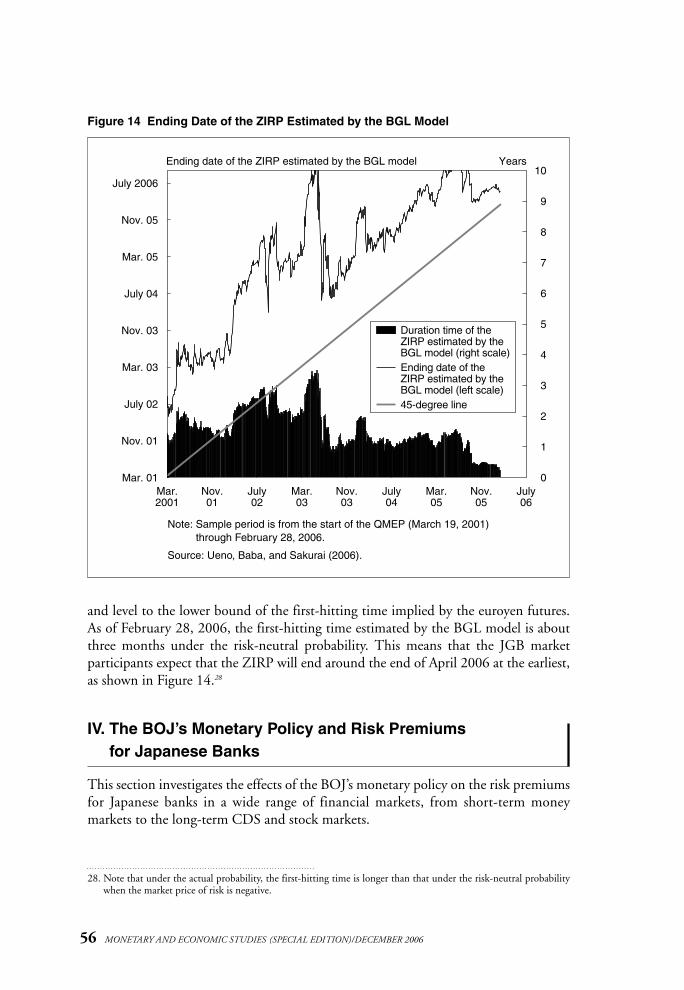
and level to the lower bound of the first-hitting time implied by the euroyen futures.As of February 28, 2006, the first-hitting time estimated by the BGL model is aboutthree months under the risk-neutral probability. This means that the JGB market participants expect that the ZIRP will end around the end of April 2006 at the earliest,as shown in Figure 14.28

IV. The BOJ’s Monetary Policy and Risk Premiums for Japanese Banks

This section investigates the effects of the BOJ’s monetary policy on the risk premiumsfor Japanese banks in a wide range of financial markets, from short-term money markets to the long-term CDS and stock markets.


Figure 14 Ending Date of the ZIRP Estimated by the BGL Model

July 2006

July06

Nov. 05

Nov.05

Mar. 05

Mar.05

July 04

July04

Nov. 03

Nov.03

Mar. 03

Mar.03

July 02

July02

Nov. 01

Nov.01

Mar. 01Mar.2001

0

1

2

3

4

5

6

7

8

9

10Ending date of the ZIRP estimated by the BGL model Years

Duration time of the ZIRP estimated by the BGL model (right scale)Ending date of the ZIRP estimated by the BGL model (left scale)45-degree line

Note: Sample period is from the start of the QMEP (March 19, 2001)through February 28, 2006.


28. Note that under the actual probability, the first-hitting time is longer than that under the risk-neutral probabilitywhen the market price of risk is negative.

A. NCD Interest Rates1. Dispersion of NCD interest rates across banksFirst, let me review the analysis by Baba et al. (2006) that explores the effects of theBOJ’s monetary policy on the NCD interest rates. Major Japanese banks recentlyraise about 30 percent of their total market funding by issuing NCDs. Thus, NCDscan be thought of as one of their principal instruments for meeting liquidity needs.

Interest rates on major banks’ newly issued NCDs had served as a main indicatorfor deregulated interest rates, although their movement had been similar across banks for some time after the first NCDs were issued in May 1979. That is, the NCD interest rates had not reflected differences in bank credit risks. From the 1990s, however, the NCD interest rates started to reflect the credit risk of individual issuingbanks, due mostly to the rising concern over the instability of the Japanese financial system. Such concern heightened during the period from late 1997 to 1998. This isshown in Figure 15 by substantial spikes in the dispersion as measured by the standarddeviation of the weekly NCD interest rates across issuing banks in November 1997.29

The standard deviations declined significantly, however, after the adoption of the ZIRP in February 1999 and fell further following the adoption of the QMEP in March 2001.30

57


Figure 15 Dispersion of NCD Interest Rates

Percent

Sep.1995

Sep.96

Sep.97

Sep.98

Sep.99

Sep.2000

Sep.01

Sep.02

Sep.04

Sep.03

0.0

0.1

0.2

0.3

QMEPZIRPPeriod offinancial crisis

Standard deviationSample average

Note: NCD interest rates used here are those with maturities less than 30 days.

Source: Baba et al. (2006).

29. The standard deviation of the NCD interest rates with maturities less than 30 days is plotted in Figure 15. It isthe most liquid maturity zone of the NCDs in Japan. Baba et al. (2006) further report a similar result for othermaturity zones including less than 60 days and 90 days. Sample banks are 11 city and trust banks for whichweekly NCD interest rates are available.

30. In calculating the averages of standard deviations, the following event dates are excluded for institutional reasons:(1) the end of 1999 (Y2K problem); (2) the end of 2000 (preparation for the adoption of real-time gross settlement [RTGS]); and (3) the end of fiscal 2001 (the partial removal of blanket deposit insurance). Evidently,significant spikes are observed on these three dates.

2. Credit curves of NCD spreadsNext, let me look at the credit curves of NCD spreads. Here, the NCD credit spreadfor a bank is defined as the interest rate on NCDs issued by the bank with maturitiesless than 30 days minus the weighted average of the uncollateralized overnight call rate.The data frequency is weekly as before. Then, Baba et al. (2006) run cross-sectionaltime-series regressions of the credit spreads on dummy variables corresponding to sample banks’ credit ratings for each of the following three years under study: (1) 1999,when the ZIRP was put in place; (2) 2002, one year after the adoption of the QMEP;and (3) 2004, the last year of their sample period. The estimation includes end-of-March, September, and December dummies to control for seasonal market tightness inannual/semiannual book-closing months and the year-end month. The credit spreadsfor each credit rating category, derived from the coefficients on credit rating dummiesalong with the constant term, map out the “credit curve” for each year.

Figure 16 demonstrates how the slope of the estimated credit curve became flatterover time.31 It seems fair to say that the credit curves flattened after the adoption ofthe ZIRP in 1999, flattened further following the adoption of the QMEP in 2002,and virtually flattened out in 2004.

The estimation result indicates that the credit risk premiums among major banksare recently close to zero, and that the differences in credit ratings among them arenow hardly reflected in their fund-raising costs in the money market, such as theNCD market. Therefore, the narrowed dispersion of fund-raising costs among banks,shown in Figure 15, is more likely to be a result of declines in risk premiums acrossthe board in the money market, rather than a result of a lowered dispersion of creditratings among major banks.


31. Sample banks are the same as in Figure 15.

Figure 16 Estimated Credit Curves of NCD Spreads

0.00

0.02

0.04

0.06

0.08

A2 A3 Baa1 Baa2

Percent

199920022004

Note: NCD interest rates are those with maturities less than 30 days. Credit ratingsare the long-term ratings of Moody’s.


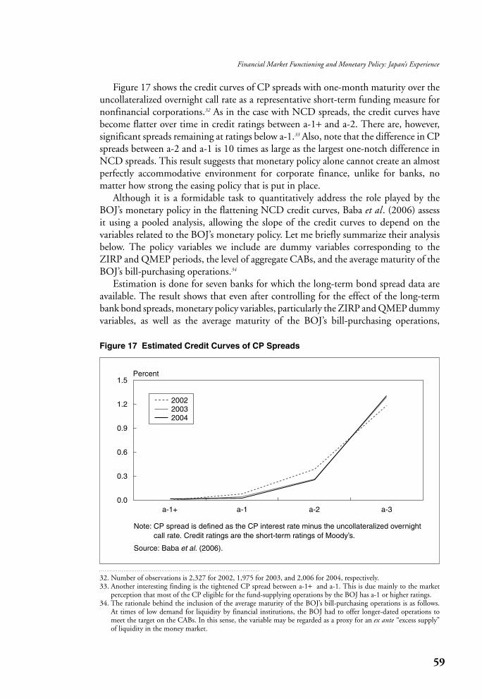
Figure 17 shows the credit curves of CP spreads with one-month maturity over theuncollateralized overnight call rate as a representative short-term funding measure fornonfinancial corporations.32 As in the case with NCD spreads, the credit curves havebecome flatter over time in credit ratings between a-1+ and a-2. There are, however,significant spreads remaining at ratings below a-1.33 Also, note that the difference in CPspreads between a-2 and a-1 is 10 times as large as the largest one-notch difference inNCD spreads. This result suggests that monetary policy alone cannot create an almostperfectly accommodative environment for corporate finance, unlike for banks, no matter how strong the easing policy that is put in place.

Although it is a formidable task to quantitatively address the role played by theBOJ’s monetary policy in the flattening NCD credit curves, Baba et al. (2006) assessit using a pooled analysis, allowing the slope of the credit curves to depend on the variables related to the BOJ’s monetary policy. Let me briefly summarize their analysisbelow. The policy variables we include are dummy variables corresponding to theZIRP and QMEP periods, the level of aggregate CABs, and the average maturity of theBOJ’s bill-purchasing operations.34

Estimation is done for seven banks for which the long-term bond spread data areavailable. The result shows that even after controlling for the effect of the long-termbank bond spreads, monetary policy variables, particularly the ZIRP and QMEP dummyvariables, as well as the average maturity of the BOJ’s bill-purchasing operations,

59


Figure 17 Estimated Credit Curves of CP Spreads

0.0

0.3

0.6

0.9

1.2

1.5

a-1+ a-1 a-2 a-3

Percent

200220032004

Note: CP spread is defined as the CP interest rate minus the uncollateralized overnightcall rate. Credit ratings are the short-term ratings of Moody’s.


32. Number of observations is 2,327 for 2002, 1,975 for 2003, and 2,006 for 2004, respectively.33. Another interesting finding is the tightened CP spread between a-1+ and a-1. This is due mainly to the market

perception that most of the CP eligible for the fund-supplying operations by the BOJ has a-1 or higher ratings.34. The rationale behind the inclusion of the average maturity of the BOJ’s bill-purchasing operations is as follows.

At times of low demand for liquidity by financial institutions, the BOJ had to offer longer-dated operations tomeet the target on the CABs. In this sense, the variable may be regarded as a proxy for an ex ante “excess supply”of liquidity in the money market.

significantly contributed to the decline in risk premiums across the board, as well as the flattening of the credit curves in the NCD market.

B. Risk Premiums for Japanese Banks in the CDS and Stock MarketsLast, let me look at the CDS market as a longer-term market for bank credit risk, aswell as the stock market. There has been widespread use of stock prices to assess thedefault probabilities for corporations using structural models that have their origin inMerton (1974). In addition, as argued by Ito and Harada (2004), due to the recentexpansion of CDS trading for Japanese banks, CDS spreads are now regarded asreflecting credit risks of Japanese banks much more sensitively than straight bondspreads and the Japan premium (the TL spread). The typical maturity of CDS contracts for Japanese entities is five years. We can use the so-called reduced-formmodel to estimate default probabilities from the CDS spreads.

Ueno and Baba (2006a, b) compute the one-year-ahead default probabilities for fourJapanese mega-banks, namely, Bank of Tokyo-Mitsubishi (BTM), Sumitomo MitsuiBanking Corporation (SMBC), UFJ Bank (UFJ), and Mizuho Bank (MIZUHO),from CDS spreads and stock prices.35 Figures 18 and 19 show the results, respectively.Evidently, from late 2001 to 2003, a large and prolonged surge is observed in both


Figure 18 Default Probabilities Implied by CDS Spreads

Oct.1998

Oct.99

Oct.2000

Oct.01

Oct.02

Oct.03

Oct.04

0.00

0.02

0.04

0.06

0.08

0.10

0.12

0.14

BTMSMBCUFJMIZUHO

Notes: 1. The time horizon is assumed to be one year. For details, see Appendix 3.2. BTM: Bank of Tokyo-Mitsubishi; SMBC: Sumitomo Mitsui Banking

Corporation; UFJ: UFJ Bank; MIZUHO: Mizuho Bank.3. SMBC, UFJ, and MIZUHO were established as a result of their respective

mergers during the sample period. Before the mergers, we use the data onSumitomo Bank for SMBC, Sanwa Bank for UFJ, and Fuji Bank for MIZUHO.

Source: Ueno and Baba (2006a).

35. Ueno and Baba (2006b) estimate the default probabilities from the stock prices using the method by Merton(1974). For the reduced-form model used in Ueno and Baba (2006a) to estimate the default probabilities fromthe CDS spreads, see Appendix 3. Ueno and Baba (2006a) also estimate expected recovery rates, jointly with thedefault intensities, using both senior and subordinated CDS spreads.

markets, in addition to 1998. This is in sharp contrast to the result of the NCD interest rate and TL spread, shown in Figures 4 and 5. Putting these results together,we can tentatively conclude that there is something distinct in the perceptions forJapanese banks in short-term money markets, compared with other markets including the CDS and stock markets.

Ueno and Baba (2006a) further explore the relationship between the “systemic”nature of Japanese bank credit risk and the government.36 Specifically, our strategy isto extract a latent common factor from the estimated default intensities for the fourbanks by factor analysis, and compare the common factor with the default intensityfor the Japanese government.37 The result is displayed in Figure 20. Surprisinglyenough, these two default risk indices are almost perfectly correlated with each other,with a correlation coefficient of higher than 0.95. Implications derived from thesefindings are discussed in the next section.

61


Figure 19 Default Probabilities Implied by Stock Prices

Aug.1999

Aug.2000

Aug.01

Aug.02

Aug.03

Aug.04

Aug.05

0.00

0.05

0.10

0.15

0.20

0.25

BTMSMBCUFJMIZUHO

Notes: 1. The time horizon is assumed to be one year. Merton’s (1974) model is used.2. BTM: Bank of Tokyo-Mitsubishi; SMBC: Sumitomo Mitsui Banking

Corporation; UFJ: UFJ Bank; MIZUHO: Mizuho Bank.3. SMBC, UFJ, and MIZUHO were established as a result of their respective

mergers during the sample period. Before the mergers, we use the data onSumitomo Bank for SMBC, Sanwa Bank for UFJ, and Fuji Bank for MIZUHO.

Source: Ueno and Baba (2006b).

36. A noteworthy feature of the CDS contracts for Japanese entities is that Japanese sovereign contracts have beentraded very actively. As shown by Packer and Suthiphongchai (2003), from 2000 to 2003 the total number of CDSquotes for Japanese sovereign bonds amounts to 2,313, which corresponds to the third largest total, after Brazil andMexico. This fact, along with successive downgrades of the credit rating on Japanese sovereign bonds, showsinvestors’ deep concern over the financial standing of the Japanese government itself, which faced prolonged deflation after the bursting of the bubble economy in the early 1990s, and the ensuing structural problems, such asthe fragile financial system.

37. The estimation result of the factor analysis shows that the first factor whose factor loadings are almost equalacross the four banks contributes more than 90 percent of the total variation of the default intensities for the fourbanks. Thus, it seems quite natural to regard this first factor as the “systemic risk (common) factor.”

V. Concluding Remarks

This paper has reviewed the financial market functioning under the ZIRP and the subsequent QMEP conducted by the BOJ. In doing so, particular attention has beengiven to assessing market perceptions about the duration of the BOJ’s monetary policyand its effects on risk premiums for Japanese banks. The main findings are as follows.

First, the estimation results of the JGB yield curve using the BGL model showthat (1) the shadow interest rate has been negative since the late 1990s, turnedupward in 2003, and has been on an uptrend since then, and (2) the first-hittingtime until the negative shadow interest rate hits zero again under the risk-neutralprobability is estimated to be about 10 months as of end-December 2005 from thefixed-parameter model, and about three months as of the end of February 2006 fromthe day-to-day calibration. Second, under the ZIRP and QMEP, the risk premiumsfor Japanese banks have almost disappeared in short-term money markets, while theyhave remained in long-term markets such as the CDS and stock markets.

Here, the next question we should address is the following: “why did the short-termmoney market prices such as the NCD interest rate and TL spread not show a surge in


Figure 20 CDS Spread-Implied Default Intensity for Japan Sovereign and CommonFactor Derived from the Four Japanese Mega-Banks’ Default Intensities

–1.5

–1.0

–0.5

0.0

0.5

1.0

1.5

2.0

2.5

3.0

0.000

0.002

0.004

0.006

0.008

0.010

0.012

Oct.1998

Oct.99

Oct.2000

Oct.01

Oct.02

Oct.03

Oct.04

Oct.05

Common factor (left scale)Japan sovereign (right scale)

Notes: 1. The common factor is derived from the four Japanese mega-banks’default intensities estimated from the CDS spreads using factoranalysis. The method of principal component is used. The result isthe initial solution before a rotation.

2. The common factor is standardized as mean zero and standard deviation one.

Source: Ueno and Baba (2006a).

the period of financial instability under the QMEP, unlike the default probabilitiesderived from the long-term CDS spreads and stock prices?” Let me conclude this paperby raising two hypotheses to address this question and briefly commenting on each.38

The first hypothesis is raised by Baba et al. (2006). That is, the participants in theJapanese money markets positively perceive the role of the BOJ’s ample liquidity provisions under the QMEP in containing the near-term defaults of banks caused bythe liquidity shortage. This hypothesis seems to be supported by the findings aboutNCD credit curves reviewed in this paper. Let me briefly comment on this issue below.

There are two possible effects of the BOJ’s monetary policy on bank credit risk. Thefirst effect is that easy monetary policy raises asset prices and lowers risk premiums.This effect is very general. But the second effect is rather specific to the QMEP conducted by the BOJ. The policy package under the QMEP, namely, the strong commitment to maintain a zero interest rate as well as the provision of ample liquidity,substantially contained the risk that banks would fail to meet short-term paymentobligations, which likely makes the near-term chance of a default smaller.

An interesting point to note here is that the default probabilities observed in thelong-term CDS and stock markets surged significantly during the period of financialinstability even under the QMEP. We also find that the common factor derived fromthe default intensities of the four Japanese mega-banks is almost perfectly correlatedwith the default intensity of the Japanese government. This empirical result may suggest the difference in the role between the government and the BOJ in addressingthe problem of financial instability around 2001 to 2003: the government played theleading role in addressing the long-term financial standing (solvency) of the Japanesefinancial institutions, while the BOJ played the role of addressing the short-term liquidity shortage of the Japanese financial institutions.

The second (negative) hypothesis is that the BOJ’s QMEP has only paralyzed thefunctioning of short-term money markets in that banks do not need to raise short-term liquidity from markets and thus do not need to evaluate their counterparties’risk properly. This is because the BOJ provided too much money to meet the target for the CABs. This hypothesis is hard to test. But Baba et al. (2005) imply thevalidity of this hypothesis, saying that as financial institutions have become more andmore dependent on the BOJ’s fund-supplying market operations, the size of the callmarket, which had already shrunk under the ZIRP, has contracted further since theadoption of the QMEP.39

63


38. In this regard, Ito and Harada (2004) raise the following two hypotheses. The first is that “Japanese banks havebeen required to put up cash collaterals to raise dollars in the money markets since around 2000–2001.” The second is that “weaker banks have exited from the international money markets.” Both of these hypotheses may bethe case, but are not necessarily verified. For instance, if the second hypothesis is the case, why did the CDS andequity markets imply high default probabilities for Japanese mega-banks until quite recently?

39. The daily trading volume in the uncollateralized call market was about ¥7.4 trillion before the adoption of theQMEP. Subsequently, it gradually declined, reaching ¥1.3 trillion in April 2004. The amount outstanding alsodeclined from ¥17.9 trillion to ¥5.0 trillion during the same period.

APPENDIX 1: GOROVOI AND LINETSKY’S ANALYTICAL SOLUTION TO THE BLACK MODEL

This appendix briefly describe the analytical solution by Gorovoi and Linetsky(2004) to the Black model of interest rates as options, as well as the framework byLinetsky (2004) to calculate the first-hitting time until the negative shadow interestrate hits zero.

A. Analytical Solution to the Black ModelWe adopt the Vasicek model for the shadow interest rate under the risk-neutral probability:

drt* = �(� − rt

*)dt + �dBt , r0* = r , (A.1)

where � is the long-run level of the shadow interest rate, � is the rate of mean reversiontoward the long-run level, and � is the volatility parameter.

Note that the discount bond price can be given by

P (r,T ) = Er[exp{−∫T

s =0rsds }] = Er[exp{−∫

T

s =0max[0, rs

*]ds }], (A.2)

where Er[•] ≡ E[•r0* = r ], and T is time to maturity. (A.2) has the form of the

Laplace transform of an area functional of the shadow interest rate diffusion:

At ≡ ∫0

tmax[0, rs

*]ds, t ≥ 0. (A.3)

The area functional measures the area below the positive part of a sample path of theinterest rate process up to time t . Thus, the discount bond price can be calculated as

P (r,T ) = Er[exp(−AT)]. (A.4)

To calculate the discount bond price (A.4), the spectral expansion approach is used.The discount bond price P (r, T ) as a function of time to maturity T, and the initialshadow interest rate r, solve the fundamental pricing partial differential equation:

1––� 2Prr + �(� − r )Pr − max[0, r *]P = PT , (A.5)2

subject to the initial condition P(r, 0) = 1. The solution has the eigenfunction expansion:

�

P (r,T ) = Er[exp(−AT)] =cn exp(−�nT )n(r ), (A.6)n =0

� 2 �(� − r )cn = ∫ (r )–– exp(− –––––––)dr. (A.7)−� � 2 � 2


65


Here, {�n}�n =0 are the eigenvalues with 0 < �0 < �1 < . . . , lim

n→��n = �, and {n}�

n =0 are thecorresponding eigenfunctions of the associate Sturm-Liouville spectral problem:

1−––� 2u′′(r ) − �(� − r )u′(r ) + max[0, r *]u (r ) = �u (r ). (A.8)2

Here, we have the following asymptotics for large times to maturities:

1lim R (r,T ) = lim(− –– ln P (r,T )) = �0 > 0. (A.9)T→� T→� T

As time to maturity increases, the yield curve flattens out and approaches the principaleigenvalue �0. Here, the principal eigenvalue is guaranteed to be strictly non-negative.

B. First-Hitting Time until the Negative Shadow Interest Rate Hits ZeroThe first-hitting time is defined as

�0 ≡ min[t ≥ 0; rt* = 0]. (A.10)

Linetsky (2004) calculates the probability distribution function (PDF) of the first-hitting time for the Vasicek process using the eigenfunction expansion method. In this paper, we use the mode value of the estimated PDF as the representative value ofmarket perceptions about the first-hitting time �.

To calculate the PDF of the first-hitting time, Linetsky (2004) uses the eigenfunctionexpansion approach. Suppose that r0

* =r < 0 and t > 0, the PDF of the first-hitting timecan be written as

�

f� 0(t ) =dn�n exp(−�nt ), t ≥ 0, (A.11)n =1

where {�n}�n =0 are the eignvalues with 0 < �0 < �1 < . . . < lim

n→��n = �. Here, {dn}�

n =0 areexplicitly given as

H�n(√�––

(� − r )/�)–ndn = − –––––––––––––––––––,�n –– –––[H�(√�

––�/�)] �nn � � = –– (A.12)n

where H�(•) denotes the Hermite function.

APPENDIX 2: FIXED-PARAMETER BGL MODELThis appendix briefly describes the basic setup for the fixed-parameter BGL modelused in Ichiue and Ueno (2006). Under the actual probability P, rt

* is assumed to follow a process given by

drt* = �P(�P − rt

*)dt + �dBtP, (A.13)

�t = �0 + �1rt*, (A.14)

where �t denotes the market price of risk. With this choice of market price of risk, rt*

follows an Ornstein-Uhlenbeck process under both the actual probability P and therisk-neutral probability Q. Specifically, under Q,

drt* = �Q(�Q − rt

*)dt + �dBtQ, (A.15)

where �Q = �P + �1� and �Q�Q = �P�P − �0�.Discretizing (A.13) gives the following transition equation:

r *t +h = � + �rt

* + �t+h , (A.16)

� = �P(1 − exp(−�Ph )), (A.17)

� = exp(−�Ph ). (A.18)

�t is assumed to be normally distributed with mean zero and standard deviation ��,where

1 − exp(−2�Ph )�� = � –––––––––––– . (A.19)

√ 2�P

Let Rt denote a five-dimensional vector with the observed interest rates at time t. Weuse the observed JGB yields with 0.5-, two-, five-, and 10-year maturities, as well asthe collateralized overnight call rate as Rt . The measurement equation for Rt is thengiven by

Rt+h = z (r *t +h) +et+h , vart(et+h) = Ht . (A.20)

Here, z (r *t +h) is a function that relates the shadow interest rate to the observed rates,

and et+h is a measurement error vector. The errors are assumed to be normally distrib-uted with mean zero and standard deviation �� for each yield, where �� is a constantto be estimated. Note that the function z (r *

t +h) is nonlinear due to the use of the BGL model.

As in Duffee (1999), we use a Taylor approximation of this function around theone-period forecast of r *

t +h to linearize the model:


67


Rt+hON = �t+hr *

t +h + et+hON, (A.21)

1, if � + �rt* ≥ 0

�t+h = , (A.22)0, otherwise

R∼

t+h = (z (� +�rt*) − � − �rt

*) + z ′(� + �rt*)r *

t +h + e∼t+h , (A.23)

where R∼

t+h is a vector of JGB yields with 0.5-, two-, five-, and 10-year maturities. The likelihood function is constructed following De Jong (2000).

APPENDIX 3: ESTIMATION METHOD OF DEFAULT INTENSITYFROM THE CDS SPREADS

This appendix describes the estimation method of default intensity from the CDSspreads used by Ueno and Baba (2006a). The model setup follows Pan and Singleton(2005). Under the actual measure P, �t

Q is assumed to follow a process given by

d�tQ = �P(�P − �t

Q )dt +�Q √––�t

Q dBtP, (A.24)

�0�t = –––– + �1√––�t

Q . (A.25)√––�t

Q

With this choice of market price of risk �t, �tQ follows a square diffusion process

under both P and Q. Specifically, under Q,

d�tQ = �Q(�Q − �t

Q )dt +�Q √––�t

Q dBtQ, (A.26)

where �Q = �P + �1�Q and �Q�Q = �P�P − �0�Q. Discretizing the CDS pricing equation40

gives the following transition equation:

�Qt+h = � + ��t

Q + �t+h , (A.27)

where � = �P(1 − exp(−�Ph )) and � = exp(−�Ph ). �t is assumed to be normally distributed with mean zero and standard deviations ��, where

1 − exp(−�Ph ) �P(1 − exp(−�Ph )) �� = �Q ––––––––––– –––––––––––––– + �t

Q exp(−�Qh ) . (A.28)√ �P 2

40. The CDS pricing equation equates the present value of the premiums paid by the buyer of CDS protection withthe present value of the payment paid by the seller when credit events occur.

Now, let CDSt denote an Nt -dimensional vector of the observed CDS spreads at timet , where N denotes the maturity of the CDS contract. The measurement equationfor CDSt is then given by

CDSt+h = z (�Qt+h) + et+h , vart(et+h) = Ht . (A.29)

Here, z (�Qt+h) maps the default intensity into CDS spreads in which we attempt to

identify between the default intensity and the expected recovery due to the property offractional recovery of face value, inherent in the CDS contract.41 We further identifythe difference in the expected recovery rate between senior and subordinated CDScontracts by assuming their proportional relation to each other. The function z (�Q

t+h) isnonlinear, and et+h is a measurement error vector. The matrix Ht is an Nt × Nt diagonalmatrix of which the j -th diagonal element is ��Bid j,t − Askj,t.

As in Duffee (1999), a Taylor approximation of this function around the one-period forecast of �t

Q is used to linearize the model and we do not assume that thedefault intensity processes are stationary. Therefore, we cannot use the unconditionaldistribution of �t

Q to initiate the Kalman filter recursion. Instead, we use a least-squaresapproach to extract an initial distribution from the first CDS spread observation.Denote this first date as date 0. Then,

z (�Q0 ) ≈ z (�Q

0 ) − Z�Q + Z�Q0 , (A.30)

where Z is the linearization of z around �Q :

z (�Q0 )Z = –––––– . (A.31)

�Q0 �Q

0 =�Q

Based on this linearization, we can write the measurement equation for the first dateCDS spreads as

CDS0 = z (�Q) − Z�Q + Z�Q0 + e0. (A.32)

This equation can be rewritten in terms of �Q0 :

Z ′(CDS0 − z (�Q) + Z�Q ) Z ′e0�Q0 = –––––––––––––––––––– − ––––. (A.33)

Z ′Z Z ′Z

Thus, the distribution of �Q0 is assumed to have mean Z ′(CDS0 − z 0(�Q) + Z�Q )/(Z ′Z )

and variance H0/(Z ′Z ). Following De Jong (2000), given this initial distribution ofunobserved default intensity, the extended Kalman filter recursion proceeds as follows.


41. For fractional recovery of face value, see Duffie and Singleton (2003) for details.

69


Model:

CDSt+h = A(�tQ ) + B (�t

Q )�Qt+h + et+h, var(et+h ) = Ht , (A.34)

A(�tQ ) = z (� + ��t

Q ) − B (�tQ )(� + ��t

Q ), (A.35)

z (�Qt+h)B (�t

Q ) = ––––––– , (A.36) �Q

t+h �Qt+h =�+��t

Q

�Qt+h = � + ��t

Q + �t+h . (A.37)

Initial conditions:

�̂0Q = Z ′(CDS0 − z (�Q) + Z�Q )/(Z ′Z ), (A.38)

q̂0 = H0/(Z ′Z ). (A.39)

Prediction:

�Qt |t−h = � + ��̂Q

t−h , (A.40)

qt |t−h = �2q̂t−h + ��2. (A.41)

Likelihood contributions:

ut = CDSt − A(�̂Qt−h) −B (�̂Q

t−h)�t |t−h, (A.42)

Vt = B (�̂Qt |t−h)qt |t−hB (�̂Q

t−h) +Ht , (A.43)

−2lnLt = lnVt+ut′Vt−1ut . (A.44)

Updating:

Kt = qt |t−hB (�̂Qt−h)′Vt

−1, (A.45)

Lt = I − KtB (�̂Qt−h), (A.46)

�̂Qt = �t |t−h + Ktut , (A.47)

q̂t = Ltqt |t−h. (A.48)

The survival and default probabilities are calculated following Longstaff, Mithal, andNeis (2005).

Baba, N., M. Nakashima, Y. Shigemi, and K. Ueda, “The Bank of Japan’s Monetary Policy and BankRisk Premiums in the Money Market,” International Journal of Central Banking, 2, 2006, pp. 105–135.

———, and S. Nishioka, “Bank Credit Risk, Common Factors, and Interdependence of Credit Risk inMoney Markets: Observed vs. Fundamental Prices of Bank Credit Risk,” inProceedings of the FourthJoint Central Bank Conference, “Risk Measurement and Systemic Risk,” 2005 (forthcoming).

———, ———, N. Oda, M. Shirakawa, K. Ueda, and H. Ugai, “Japan’s Deflation, Problems in theFinancial System, and Monetary Policy,” Monetary and Economic Studies, 23 (1), Institute forMonetary and Economic Studies, Bank of Japan, 2005, pp. 47–111.

Baz, J., D. Prieul, and M. Toscani, “The Liquidity Trap Revisited,” Risk, September, 1998, pp. 139–141.Bernanke, B., “Deflation: Making Sure ‘It’ Doesn’t Happen Here,” remarks before the National Economists

Club, Washington, D.C., November 21, 2002.———, and V. Reinhart, “Conducting Monetary Policy at Very Low Short-Term Interest Rates,” speech

presented at the Meeting of the American Economic Association, San Diego, California,January, 2004.

———, ———, and B. Sack, “Monetary Policy Alternatives at the Zero Bound: An EmpiricalAssessment,” Brookings Papers on Economic Activity, 2, 2004, pp. 1–78.

Black, F., “Interest Rates as Options,” Journal of Finance, 50 (5), 1995, pp. 1371–1376.Bomfim, A., “Interest Rates as Options: Assessing the Markets’ View of the Liquidity Trap,” working

paper, Board of Governors of the Federal Reserve System, 2003. Cox, J., J. Ingersoll, and S. Ross, “A Theory of the Term Structure of Interest Rates,” Econometrica,

53 (2), 1985, pp. 385–407.De Jong, F., “Time-Series and Cross-Section Information in Affine Term Structure Models,” Journal

of Economics and Business Statistics, 18 (3), 2000, pp. 300–318.Duffee, G., “Estimating the Price of Default Risk,” Review of Financial Studies, 12 (1), 1999,

pp. 197–226.Duffie, D., and K. Singleton, Credit Risk, Princeton: Princeton University Press, 2003.Gorovoi, V., and V. Linetsky, “Black’s Model of Interest Rates as Options, Eigenfunction Expansions

and Japanese Interest Rates,” Mathematical Finance, 14, 2004, pp. 49–78.Hicks, J., “Mr Keynes and the Classics: A Suggested Interpretation,” Econometrica, 5, 1937, pp. 147–159.Ichiue, H., and Y. Ueno, “The Monetary Policy Effects under the Zero Interest Rate: A Macro-Finance

Approach with Black Model of Interest Rates as Options,” Bank of Japan Working Paper No. 06-E-16, Bank of Japan, 2006.

Ito, T., and K. Harada, “Credit Derivatives Premium as a New Japan Premium,” Journal of Money,Credit and Banking, 36 (5), 2004, pp. 965–968.

———, and ———, “Bank Fragility in Japan: 1995 to 2003,” in Michael M. Hutchison and FrankWestermann, eds. Japan’s Great Stagnation: Financial and Monetary Policy Lessons for AdvancedEconomies, Cambridge, Massachusetts: The MIT Press, 2006.

Keynes, J., The General Theory of Employment, Interest, and Money, New York: Macmillan, 1936.Krugman, P., “Japan’s Trap,” 1998 (available at http://www.mit.edu/krugman/www/japtrap.html).Linetsky, V., “Computing Hitting Time Densities for OU and CIR Diffusions: Applications to Mean-

Reverting Models,” Journal of Computational Finance, 7 (4), 2004, pp. 1–22.Longstaff, F., S. Mithal, and E. Neis, “Corporate Yield Spreads: Default Risk or Liquidity? New

Evidence from the Credit-Default Swap Market,” Journal of Finance, 60 (5), 2005, pp.2213–2253.

McCulloch, J., “Measuring the Term Structure of Interest Rates,” Journal of Business, 44 (1), 1971, pp. 19–31.

Merton, R., “On the Pricing of Corporate Debt: The Risk Structure of Interest Rates,” Journal ofFinance, 29 (2), 1974, pp. 449–470.

Nakayama, T., N. Baba, and T. Kurihara, “Price Developments of Japanese Government Bonds in 2003,”Market Review, Paper No. 2004-E-2, Financial Markets Department, Bank of Japan, 2004.


References

71

Comment

Nishioka, S., and N. Baba, “Credit Risk Taking by Japanese Investors: Is Skewness Risk Priced in JapaneseCorporate Bond Market?” Bank of Japan Working Paper No. 04-E-7, Bank of Japan, 2004.

Oda, N., and K. Ueda, “The Effects of the Bank of Japan’s Zero Interest Rate Commitment andQuantitative Monetary Easing on the Yield Curve: A Macro-Finance Approach,” CARFDiscussion Paper No. F-013, University of Tokyo, 2005.

Packer, F., and C. Suthiphongchai, “Sovereign Credit Default Swaps,” BIS Quarterly Review, Bank forInternational Settlements, December, 2003, pp. 81–88.

Pan, J., and K. Singleton, “Default and Recovery Implicit in the Term Structure of Sovereign CDSSpreads,” working paper, Stanford University, 2005.

Robertson, D., Money, Cambridge Economic Handbooks, 1948.Rogers, L., “Which Model for Term Structure of Interest Rates Should One Use?” Proceedings of IMA

Workshop on Mathematical Finance, 65, Institute for Mathematics and Its Applications, NewYork: Springer-Verlag, 1995, pp. 93–116.

———, “Gaussian Errors,” Risk, 9 (1), January, 1996, pp. 42–45.Ueda, K.,“The Bank of Japan’s Struggle with the Zero Lower Bound on Nominal Interest Rates:

Exercises in Expectations Management,” International Finance, 8 (2), 2005, pp. 329–350.Ueno, Y., and N. Baba, “Default Intensity and Expected Recovery of Japanese Banks and ‘Government’:

New Evidence from the CDS Market,” Bank of Japan Working Paper No. 06-E-04, Bank of Japan, 2006a.

———, and ———, “Price Discovery for Financial Standing of Japanese Banks: A Comparisonbetween the CDS and the Stock Markets,” mimeo, Bank of Japan, 2006b.

———, ———, and Y. Sakurai, “The Use of the Black Model of Interest Rates as Options forMonitoring the JGB Market Expectations,” Bank of Japan Working Paper No. 06-E-15, Bankof Japan, 2006.

Vasicek, O., “An Equilibrium Characterization of the Term Structure,” Journal of Financial Economics,5, 1977, pp. 177–188.

Comment

DAVID LONGWORTH42

Bank of Canada

I. Introduction

In his interesting paper, Naohiko Baba covers two main subjects. The first is expecta-tions about interest rates rising above the zero bound. The second is risk premiums for Japanese banks during the period of the zero interest rate policy (ZIRP) and thequantitative monetary easing policy (QMEP). The paper is very useful in providing uswith a summary of the extensive work that has been done at the Bank of Japan (BOJ)by the author and various co-authors on related topics over the past three years.

I would like to focus on four topics:• What we can learn from this paper about yield curve indicators and how financial

markets work at the zero lower bound on nominal interest rates.• What we can learn from this paper about the behavior of credit risk premiums

for banks under the ZIRP and QMEP.

42. The views expressed in this comment are solely those of the author. No responsibility for them should be attributedto the Bank of Canada.


• What we can learn about monetary policy at the zero bound.• What some of the extensions to the analysis in this paper are that would help us

to learn more about monetary policy and the behavior of financial markets atthe zero bound. I will talk about such extensions throughout my remarks.

However, before getting into these topics, I would like to step back and suggesthow, in general, I see the influences on financial markets.

First, it is clear that behavior in financial markets is affected by the monetary policy that is in place. In the present paper, this means the ZIRP and QMEP. Moreover,it is not merely the policy itself, but the market’s perceptions of what that policy meansin practice. In particular, the market will be influenced by publications and statementsof officials from the BOJ, as well as statements from government spokespeople. In addition, the market’s response to data will depend on how it perceives the monetarypolicy regime.

Second, the market’s perception of the credit risk it faces in lending to banks willdepend on its perception of the regulatory and supervisory system in place. In theperiod in question in Japan, this includes beliefs about the degree of forbearance ofdeficient capital positions by the supervisor and the government.

Third, changes in risk perception and risk aversion can also lead to changes infinancial market prices.

Given that all three factors above will always be at play, developing a completely“causal” story for the behavior of interest rates may be somewhat complicated. As well,some of the influences may emanate from abroad. To take two examples, changes in risk aversion or risk appetite may be international in scope and some of the data relevant to future policy interest rate developments in Japan may be data on foreigndemand or output, because that will ultimately be reflected in foreign demand forJapanese products. As evidence that the former may have been important, one canpoint to the general decline in credit spreads across countries in recent years. As evidence of the latter, one can point to the high correlation between Japanese and U.S.or German 10-year bond yields over the past five or six years, as shown in Figure 3 inthe paper.

II. Financial Markets at the Zero Bound: The Yield Curve

In the first part of the paper, the author uses the Black-Gorovoi-Linetsky (BGL)model to examine yield curve behavior when short-term interest rates are essentiallyzero. He finds that over most of the period, the BOJ was not expected to exit theZIRP or QMEP very soon. Anthony Richards, the other discussant for this paper,discusses the BGL model in more detail. What I will do is to raise two questions andtalk about possible extensions.

The first question is a technical one. If one is interested in developing precise estimates of the horizon to leave the zero bound—the “first-hitting time” in the expression used by the author—would it help to include more points along the shortpart of the yield curve, say, by adding the three-month, nine-month, 1.5-year, and 2.5-year rates?

The second question is about the interpretation of the results. As I read the resultsin Figure 13, the market has almost always underestimated the amount of time itwould take for interest rates in Japan to rise above zero. If one assumes that this risewill occur in the second half of 2006, there are basically only two periods in whichthe market has not underestimated the amount of time. The first was in mid-2003,when the market thought it would take some three to 3.5 years for rates to rise abovezero. The second was in mid-2005, when the market thought it would take one to1.5 years.

There are two extensions to this part of the paper that I would find useful. The first would be very easy to do. It is to calculate the expectation of the increase

in interest rates over the course of the first year following the first-hitting time. Thiscould be presented either as the expected one-year rate at the first-hitting time or theexpected overnight rate one year after the first-hitting time. Either would represent ameasure of the market’s view of how steep or shallow the increase in interest rateswould be in the period just after the BOJ exits zero interest rates.

The second would be to examine what macro variables and announcements aredriving the yield curve, especially the “shadow interest rate” and the first-hitting time.The author notes that “the shadow interest rate seems to have closely followed thecore CPI inflation rate with several-month lags since early 2001” (Section III.C.1)and that “the release of the CPI data is delayed by approximately two months”(Footnote 22). The relationship between the shadow interest rate and core CPI inflationis displayed graphically in Figure 11 (2) of his paper. A beginning to a further examination would be to explore more fully, in a regression context, the relationshipbetween the shadow interest rate and lags on the core CPI inflation rate. To this relationship could be added information on real growth rates in Japan, announcementsand speeches by the BOJ and government officials on monetary policy (going beyondthe announcements of the beginning of the ZIRP and QMEP), any importantannouncements on the health of the banking system, and possible foreign economicdata as well, because of its effect on the demand for Japanese goods and services. An alternative to this line of exploration would be to explore the relationship betweenthe first-hitting time and the variables that I have mentioned. I will come back to thisgeneral issue later, in the context of using estimated macro-finance models to betterunderstand the implications for monetary policy at the zero bound.

III. Financial Markets at the Zero Bound: Credit Risk Premiums

In the second part of his paper, the author turns his attention to the credit risk premiumspaid by banks. His results are not unexpected. To summarize, bank short-term risk premiums have almost disappeared, but long-term risk premiums have remained,although they are now much lower than in the 2001–03 period. The author notes(Section IV.A.2) that he and co-authors have found that “even after controlling for theeffect of the long-term bank bond spreads, monetary policy variables . . . significantlycontributed to the decline in risk premiums across the board, as well as the flatteningof the credit curves in the NCD [negotiable certificates of deposit] market.” What is

73

Comment

not controlled for, however, is the policy of the banking supervisor and the governmenttoward the operations of Japanese banks with capital deficiencies.

To the extent that there is regulatory forbearance, it may be regulatory policy asmuch as monetary policy that is leading to low credit risk premiums. Not being anexpert on the timing of various regulatory initiatives in Japan, I am unable to say howrelevant this has been over the past few years. But it certainly has had relevance oversome of the last 15 years in Japan. What we do know is that the provision of liquidityby a central bank cannot by itself make an insolvent bank solvent. Short-term creditrisk premiums presumably are more related to the expected probability of insolvencythan to liquidity, although—admittedly—excess liquidity may hide solvency problemsfrom the market to some extent. Overall, it would be useful for the author to spendsome time to see whether the analysis is robust to an examination of the attitude of thesupervisor and the government toward capital deficiencies in Japanese banks over theperiod in question.

IV. Monetary Policy at the Zero Bound

I would now like to turn my attention to the question of how monetary policy canand has worked at the zero bound for nominal interest rates.

From a theoretical point of view, there are various channels through which monetarypolicy can work at the zero bound. The first channel is engendering expectations thatrates will stay at zero for a long time, or until some condition is fulfilled, such as the“commitment” under the QMEP “to maintain the policy until the year-on-year rate of change in the core CPI . . . registers zero percent or higher on a sustainable basis.”This first channel is, in essence, the topic of the first half of the paper. The second channel is working through quantities, such as under the QMEP, assuming that moneyand other financial assets are imperfect substitutes. The QMEP presumably wasexpected to reduce risk premiums of various sorts, the topic of the second half of thepaper, and to raise asset prices and thus wealth. Other quantitative policies include theuse of foreign exchange market intervention to affect foreign exchange rates. The thirdchannel is by working in conjunction with fiscal policy, such that an increase in fiscalspending is financed by printing money. (Some of these topics were dealt with byBennett T. McCallum earlier in the conference.)

The paper clearly shows that the first channel has been an important one in the case of Japan—expectations of a significant period of zero interest rates were indeedengendered and long-term rates came down significantly as a result. As mentioned earlier, however, the expected period over which interest rates would remain at zero was,with two brief exceptions, shorter than the actual period over which interest rates haveremained at zero. And so the question remains, is this because the BOJ underestimatedthe depth of the deflationary problem, or because the market misunderstood how longthe BOJ would indeed have to keep interest rates at zero?

To understand more fully what was driving changes in the market’s expectation ofthe time that interest rates would be at zero, it is imperative to use models that relatethe macroeconomy to the yield curve. As the author would be the first to argue, such


work needs to explicitly take into account the existence of the zero bound. The authoris critical of earlier work by Bernanke, Reinhart, and Sack (2004) and Oda and Ueda(2005) because it relies on specific macroeconomic structures and does not closely tracethe actual Japanese government bond yield curve. While the macro-finance framework,in which a macro-model structure is added to a yield curve model, is still in its infancy,I would argue that something like it is needed to understand the effects of a monetarypolicy framework on the yield curve, as well as how macroeconomic shocks and “news”affect the yield curve. Indeed, as one who grew up as a macroeconomist, I found itsomewhat strange how yield curve analysis in finance was completely divorced frommonetary policy and macroeconomic models. But now progress is being made on integration of the two fields, and it is all to the good.

Since the work by Bernanke, Reinhart, and Sack (2004) and Oda and Ueda (2005),there have been a number of developments. First, more data on the Japanese economyunder the QMEP have become available. Second, more work on what drives the yieldcurve in other economies has become available, including that of Bikbov and Chernov(2006) for the U.S. economy and that of Chabi-Yo and Yang (2006) for Canada.Third, more economists, such as Naohiko Baba, who can incorporate the nonlinearcomplications posed by the existence of the zero lower bound into the other new developments in the literature, have been entering the field everyday. Thus, I wouldcall for more work in the macro-finance area for Japan.

The paper clearly shows the credit risk premiums paid by the banks on short-termNCDs were clearly squeezed. To determine the effect of this channel of monetarypolicy on the real economy and economic activity, one needs to answer a few questions. First, how much was actually transacted at these rates, say, as a percentageof bank loans outstanding? Second, what is the evidence that more loans were madebecause of lower funding costs? For example, did interest rates on bank loans declinein the QMEP period relative to the ZIRP period? Third, what is the overall judgment as to whether this had an appreciable effect on the cost of capital for firms,and thus led to more business fixed investment than would otherwise have been thecase? As mentioned earlier, there is the question of how much of the decline in NCDrates arose because of the QMEP and how much because of regulatory forbearanceby supervisors or the government.

I would add that the whole question of the interaction of monetary and bank regulatory policies in the ZIRP and QMEP periods is one of great interest in terms ofthe policy lessons to be drawn from these periods.

V. Conclusion

The author is to be congratulated for introducing a number of tools to describe thebehavior of financial markets under the ZIRP and QMEP. In this paper, we learnmuch about the channels through which monetary policy has worked in a very lowinterest rate environment. At the same time, I would make a plea for extensions tothis work. Chief among the extensions would be to relate the changes in the Japaneseyield curve and the bank credit risk premiums to news arising from economic data,

75

Comment

information about monetary policy, and information about regulatory forbearance.Some of this work needs to be carried out in well-developed macro-finance models.


Bernanke, B., V. Reinhart, and B. Sack, “Monetary Policy Alternatives at the Zero Bound: An EmpiricalAssessment,” Brookings Papers on Economic Activity, 2, 2004, pp. 1–78.

Bikbov, R., and M. Chernov, “No-Arbitrage Macroeconomic Determinants of the Yield Curve,” paperpresented at the Annual Conference of the Bank of Canada, May, 2006.

Chabi-Yo, F., and J. Yang, “Estimating the Term Structure with Macro Dynamics in a Small OpenEconomy,” paper presented at the Annual Conference of the Bank of Canada, May, 2006.

Oda, N., and K. Ueda, “The Effects of the Bank of Japan’s Zero Interest Rate Commitment andQuantitative Monetary Easing on the Yield Curve: A Macro-Finance Approach,” CARFDiscussion Paper No. F-013, University of Tokyo, 2005.

References

Comment

ANTHONY RICHARDS

Reserve Bank of Australia

The paper by Naohiko Baba covers a wide range of material on recent developments in Japanese financial markets and provides some excellent background for this conference. Given the current policy juncture in Japan, the paper is very timely. And I found the results of the paper to be quite plausible. These comments will focus onSection III, which is the novel part of the paper, and is about modeling interest rateswhen you are at the zero lower bound. This topic is highly relevant, given that interestrates have been at or near zero in Japan for more than 10 years (i.e., since the target forthe policy rate was lowered to 0.5 percent in 1995) but as of the time of the conferencewere widely expected to rise shortly. Then I will touch briefly on some of the materialin Section IV on some broader developments in Japanese financial markets.

In contrast with earlier work by the Bank of Japan (BOJ) on the term structure, the analysis of the zero lower bound in the current paper does not start from a macro-economic model. Instead, it relies on continuous-time interest rate modeling, wherethe results are all derived from the level, shape, and volatility of the yield curve, and the assumed stochastic model. This presumably has both pluses and minuses. If wesimply want to fit the yield curve, it may be best to do so without the constraints that macroeconomics might add. But if we are looking for an economic interpretationof the results, we have to look outside the pure modeling exercise.

The results suggest that, as of late 2005, an increase in official interest rates wasexpected within a year. And as of February 2006, the likely date for this had moved forward somewhat. As far as the zero interest rate policy (ZIRP) is concerned, the resultssuggest that the end is nigh. Market commentary around the time of the conferencewould not suggest any reason to question this view.

To obtain the key results, the paper uses a complex continuous-time model, whichtakes account of the fact that currency represents an option that prevents interest

rates from going negative. One obvious question would be whether one could getsimilar results using a simpler framework. After all, the expectations model of theterm structure still holds even when interest rates are at the zero lower bound.

If one does some simple figuring based on the term structure, one obtains esti-mates that are reasonably consistent with expectations from surveys of economists.43

Furthermore, Figure 13 of the paper shows a comparison of the expected length ofthe ZIRP derived from the model, and two estimates derived from the euroyenfutures strip. The latter two estimates can be viewed as differing in terms of theassumptions about the size of the first BOJ move and the various risk premiums inthe futures strip. There is a fairly high correlation between the movements (but notnecessarily the levels) of the estimates from the simple approach and the estimatederived from the more complex model. This is not surprising given that the inputdata for the two different methodologies are quite similar.

So why use a more complex model? One reason is that euroyen futures only go outabout two or three years. Another reason is that the standard approach does not reallyallow simulations. So the simple approach may be all a BOJ watcher needs, but themore complex approach may be useful for a range of modeling exercises, includingpricing interest rate derivatives.

The current paper uses an insight from Fischer Black’s last paper (Black [1995]). In a liquidity trap, the equilibrium nominal interest rate that would equate savings and investment would be negative. However, assuming that currency exists (and that itcannot be taxed so that it yields a negative nominal rate of return), the zero nominalreturn on currency will dominate the negative rate that would be earned on loans. So people will not lend money at negative rates, and we will not observe them. Blackused the term “shadow” interest rate for the interest rate that would clear the market.When interest rates are positive, the shadow and actual rates are one and the samething. But when the shadow rate is negative, we do not observe it. Instead, we justobserve a zero actual rate.

Standard theoretical interest rate models have a great deal of trouble with the zerolower bound. Such models typically assume a mean-reverting component (which inthis case would tend to pull the interest rate upward), plus a stochastic component(that could take rates either up or down). But with interest rates at zero, the possibilityof downward movements is hard to deal with. Indeed, the paper notes that in practicestandard models do not do a very good job—by themselves—of tracing the changingshape of the Japanese government bond yield curve. However, the results of the papersuggest that when you instead assume that such stochastic models apply to the shadowinterest rate, and that the observed interest rate is the maximum of zero and the shadow rate, then you can explain the Japanese data pretty well.

The results suggest that the shadow interest rate was at its lowest around the secondquarter of 2003. Similarly, the “first-hitting time” (which is the estimated time until

77

Comment

43. This would involve taking the euroyen futures strip (or implied forward rates from any fitted yield curve). Thenone makes some assumptions about the credit and term risk premiums (which are presumably small) incorporatedin the futures strip. This yields an expectation about the future level of the policy rate. Then, with assumptionsabout the size of the possible move that the BOJ might undertake, one can come up with estimates of when theBOJ might increase its policy rate from zero.

the shadow rate turns positive) was at its longest around that time. Not surprisingly,this was when market yields were at their lowest levels. It was also around the time thatinflation was at its lowest point. Then, as core inflation began to rise and the economicrecovery became more entrenched, expectations about the duration of the ZIRP weregradually wound back. These results are not surprising given that the BOJ’s intentionsabout future policy have been mostly expressed in terms of the level and outlook forcore inflation.

Overall, the modeling results seem quite plausible. Now, at the risk of focusing onthem more than might have been intended, I will ask how one should think about theestimates of the shadow interest rate. Perhaps one should not focus too much on anyparticular numerical estimates, but it certainly is tempting, given that it is somethingthat comes out of the current model, and I am not aware of any other work thataddresses this question.

Figure 11 suggests that, as of mid-2003, the shadow interest rate had gotten as lowas –6 or –7 percent.44 At that time, the model suggests that the ZIRP was expected to last a further three years or so. This may actually turn out to have been very close to the mark!

The first thing to point out is that there is no macroeconomic analysis involved inthe estimate of the shadow interest rate (or the first-hitting time). Instead, it is basedpurely on the data for the yield curve and the stochastic model assumed for theshadow rate.

Now without being an expert in continuous-time finance, it is hard to be certainexactly how the model generates this shadow rate, but here is my guess. As was notedearlier, the model’s shadow interest is assumed to show some tendency to revert backto a long-run level (plus there is also a stochastic component). In the current case, thefixed-parameter model results in Figure 11 tell us that the short rate is reverting to a long-run level of 3.9 percent (although the day-to-day calibration exercise suggestsa somewhat lower rate).

Now in most countries, the shadow short rate is also the actual short rate and itwill typically not be more than a few percentage points away from its long-run level.But in the case of Japan, the shadow rate might conceivably have gotten a lot furtherfrom its long-run level.

And back in mid-2003, the term structure of the yield curve implied that theshadow rate would remain negative for about three years. If the shadow rate had atendency to revert to a mean of about 4 percent, and if it was expected to take solong for the shadow rate to rise to zero, it must have been starting a long way belowzero. So based on the yield curve of that time and the estimated parameters, themodel is apparently telling us that the only way the mean-reverting shadow ratecould have remained negative for three years was if it started off at –6 or –7 percent.So if one thought that this was too low, one would have to find some way to dampenthe effect of the mean reversion term.

How plausible are these estimates of the shadow rate? Perhaps a Taylor rule-typecalculation could shed some light on this, subject to the assumption that this type of


44. Indeed, in Ueno, Baba, and Sakurai (2006) the shadow rate appears to get even lower.

calculation remains appropriate even in extreme situations like the Japanese case.The original Taylor (1993) rule suggested that the nominal policy rate might be

set equal to the long-run equilibrium real interest rate plus the rate of inflation (eithercurrent or expected), and a response coefficient to the extent that output differs frompotential or inflation deviates from the target rate, with Taylor originally suggestingequal response coefficients of 0.5 on each gap (based on U.S. data). Suppose that thelong-run equilibrium real interest rate for Japan is around 2 percent and that theimplicit longer-term inflation target was 1 percent. The output gap is notoriously hardto measure, but based on the BOJ’s recent work it might be plausible to assume that it was something like –3 or –4 percent in mid-2003.45 And core inflation was running at around –0.5 percent at that time. If we take Taylor’s original coefficients, we cansimply add the two gaps together (say, a total of –5 percentage points) and apply a coefficient of 0.5, and add this to 0.5 percent. The result, –2 percent, falls far short ofthe estimated shadow policy rate of –6 or –7 percent. However, if one instead tooklarger response coefficients, say, as high as 2, then one could indeed generate the largenegative shadow rate derived in the current paper.46

So although my initial reaction was that a shadow rate of –6 or –7 percent seemeda bit large, one has to say that it is very hard to know how to assess something like this.How can we know what the interest rate would have been in a world so different fromours? Perhaps it would have been necessary to have both nominal and real interest rates very significantly negative to have induced Japanese consumers and firms tospend and borrow more.

Returning to the current situation, I wonder if the concept of the shadow interestrate might not have a corollary in the problems that the BOJ may have faced in managing market expectations. Usually the central bank can set the short rate at thelevel it thinks is appropriate for the economy. Indeed, some of the models assessingcentral bank transparency assume that one of the ways that the market infers the central bank’s reading of the economy is from its setting of the short rate. However, in a case like the Japanese one, the zero lower bound constrains the central bank fromsetting the policy rate at the level it thinks is appropriate, so markets are unable to inferanything from the level of the policy rate.

Of course, the BOJ can rely on other channels of communication. Its targets for quantitative variables (such the level of current account balances or open marketpurchases) might be able to replicate much of the information usually provided via a policy rate. And it also has the standard tools of speeches, policy statements, and so on to signal its views on the economy and the policy outlook. So I suspectthat the unobservability of the shadow rate has not been a major constraint on itsability to communicate with markets and the public. Of course, given that centralbank watchers always want more information from the central bank, I am sure

79

Comment

45. The relevant output gap is in relation to normal levels of resource. This is consistent with the BOJ’s recent work,rather than maximum levels as was the case in earlier BOJ estimates of the output gap.

46. However, it is noteworthy that a Taylor-type calculation would suggest that the shadow rate should have been atits lowest point about a year earlier than implied by the financial market pricing. Core inflation and GDP growthwere both significantly weaker in mid-2002 than in mid-2003: this was true for both the actual year-end data andfor forward-looking expectations from Consensus Forecasts.

they would have been happy to also have had estimates of the shadow rate as an additional guidepost.

I am now going to touch briefly on the results in Section IV. These results suggestthat markets are not discriminating much between assets of different levels of risk.This is based on a range of evidence, including on the pricing of certificates ofdeposit (CDs) issued by a sample of 11 city and trust banks that shows althoughlower-rated banks do pay a premium (Figure 15), it is now very small and lower thanin earlier years (Figure 16). There is more evidence of differentiation in the pricing ofrisk for lower-rated corporate borrowers in the CP market (Figure 17). There is alsoevidence of greater longer-term credit risk for banks implicit in the pricing of creditdefault swaps and bank equities (Figures 18–20). However, the extent of greater pricing of risk should not be overstated, given that Figure 6 shows that the spread on BBB-rated bonds has recently been only about 25 basis points, which is wellbelow equivalent spreads in other countries.

The paper tentatively suggests that one factor behind these results could be thatthe market treats the quantitative monetary easing policy (QMEP) as having more orless guaranteed the ability of large banks to meet their short-term obligations.Another proposed explanation—and these are not mutually exclusive—is that underthe QMEP, banks have not really had to go to the market to raise funds, so the CDmarket (and the money market more broadly) have atrophied and no longer reallyprice risk.

One could be disapproving of these developments. However, I am not sure oneshould criticize the BOJ if indeed this is what has happened. Over the past severalyears, its most important task was presumably to get the macroeconomy going,at almost any cost. As the paper notes (Section I), an important element of monetarypolicy has been “to alleviate concerns over the financial-sector problems . . . [M]any ofthe BOJ’s market operations had the dual role of providing ample liquidity andaddressing problems in the financial sector. In the process, the BOJ assumed a certainamount of credit risk.”

While the monetary and financial policies that have been followed have presumablyensured a more rapid recovery for the Japanese economy, they might not have donemuch for financial market development. No doubt in the period ahead, with themacroeconomic situation much improved, it will become more important to worry(again) about these more micro factors.


Black, Fischer, “Interest Rates as Options,” Journal of Finance, 50 (5), 1995, pp. 1371–1376.Taylor, John B., “Discretion versus Policy Rules in Practice,” Carnegie-Rochester Conference Series on

Public Policy, 39, 1993, pp. 195–214.Ueno, Yoichi, Naohiko Baba, and Yuji Sakurai, “The Use of the Black Model of Interest Rates as Options

for Monitoring the JGB Market Expectations,” Bank of Japan Working Paper No. 06-E-15, Bankof Japan, 2006.

References

81

General Discussion

General Discussion

Naohiko Baba responded first to discussants’ comments about the relationshipbetween the Bank of Japan’s (BOJ’s) monetary policy and the Japanese governmentbond (JGB) yield curve. Regarding the underestimation of the first-hitting time bythe JGB market, he emphasized the role of a central bank’s communication withfinancial markets, based on his experience of JGB market monitoring. He claimedthat the JGB market had always been testing the BOJ by reacting to news aboutmacroeconomic conditions to learn the BOJ’s intent and judgment about the timingof the zero interest rate policy (ZIRP) termination. In such a process, the duration of the ZIRP might be expected by the JGB market to be shorter than the actual duration. Regarding the comment about macroeconomic implications, he agreed that it would be very promising to investigate the relationship between the shadowinterest rate or first-hitting time implied by the Black-Gorovoi-Linetsky (BGL)model and macroeconomic news. As for the choice of the complicated BGL modelinstead of simple methods using euroyen futures interest rates, he pointed out someadvantages of the BGL model over the simple model. He argued that the euroyenfutures interest rate might not properly reflect market views about the future state ofthe real economy due to its relatively short maturities and it therefore became veryvolatile due to speculative trading activities.

Second, regarding the risk premiums for banks, Baba argued that not only theBOJ’s policy but also the government’s policy was very important in lowering the riskpremiums for banks during the ZIRP and quantitative monetary easing policy(QMEP) periods. He noted, however, that the government had played a leading rolein addressing the long-term financial standing—that is, solvency problems of banks—mainly through the injections of capital into banks. On the other hand, the BOJ hasplayed a leading role in addressing the short-term liquidity shortage problem of banksby supplying ample liquidity under the QMEP. He further argued that regulatory forbearance by the government also played a role in addressing the liquidity problem,particularly by postponing lifting of the full protection of bank deposits that had been planned to be in place by March 2001. Regarding whether or not the benefits of lowered risk premiums for banks were passed on to borrowers, he argued that thebenefit from the lowered short-term fund-raising cost was surely passed on by the lowered lending interest rates, while one had to wait until quite recently to see a rise inthe amount of loans.

There were several comments from participants regarding the relationship betweenthe options approach adopted by Baba and the macroeconomic approach including themacro-finance approach. Jan Marc Berk (De Nederlandsche Bank) claimed a possibleinconsistency between these two approaches when what Baba used in his approach tothe macro level is aggregated. Kiyohiko G. Nishimura (Bank of Japan) pointed out the usefulness of exploring the magnitude of the differences in the estimation errors bothin-sample and out-of-sample between the options approach and the macro-financeapproach. Glenn D. Rudebusch (Federal Reserve Bank of San Francisco) emphasizedthe role of interest rate expectations, given output and inflation forecasts under the oldregime versus the new regime such as the ZIRP and QMEP, in the context of the Taylor

rule, for instance. Maurice Obstfeld (University of California at Berkeley) pointed outthat we should look at the real interest rate in thinking about the relationship betweensavings and investment. Tao Wu (Federal Reserve Bank of Dallas) mentioned that itwould be useful to extend the model by adding macroeconomic variables or a two-factor setting. Kazumasa Iwata (Bank of Japan) paid particular attention to the meaning of the estimated long-run mean of the shadow interest rate because of theimplication for the role of the commitment under the QMEP.

Baba responded to these comments by stressing the distinct features of the JGByield curve, in that the short end of the JGB yield curve has been zero for several yearsand the shape of the yield curve was extremely flattened over the short-term andmedium-term maturity zones. Given this situation, the options approach would bevery useful for tracing the real-life shape of the yield curve and gauging the duration of the ZIRP expected by the market using high-frequency data such as a daily basis. In particular, conventional macro-finance models cannot address the latter issue. He also argued that Fischer Black’s own interpretation of the negative shadow interestrate, the liquidity trap, might have confused macroeconomists. This was becausemacroeconomists think about the liquidity trap in terms of the real interest rate in relation to the investment-savings (IS) gap, while Black thought about it in terms ofthe nominal interest rate. He claimed that this was the reason why he adopted his own interpretation: as long as the shadow interest rate was negative, JGB market participants would expect the zero nominal interest rates to continue. In this regard, he agreed with the usefulness of rigorously analyzing the relationship between macro-economic variables such as the output gap and the shadow interest rate in real terms,explicitly taking account of the consumer price index (CPI) inflation process. Lastly, he mentioned that the extension of the BGL model into a multifactor setting would be useful, while one would have to overcome some technical problems due to the lackof analytical solutions for such extensions.

There were some comments regarding the banking sector and the financial market.Andrew Filardo (Bank for International Settlements) asked about the nature of the distortions that might have arisen in these short-run funding markets as risk premiumswere squeezed in recent years in the zero interest rate environment. Hiroshi Fujiki(Bank of Japan) pointed out that we should have a better understanding about howand why bank lending did not work as a significant channel for economic recovery.Stefan Ingves (Sveriges Riksbank) argued that we should consider carefully how wecould combine the liquidity issues managed by a central bank with the solvency issuesnormally handled by a deposit insurance agency or the ministry of finance. Hung Tran(International Monetary Fund) argued that to gauge the change in market perceptionof credit risk for banks under the QMEP, the focus should be on using a credit defaultswap (CDS) spread, which would be a pure, and thus more reliable, reflection of market perception of credit risk.

The chairperson, Hiroshi Nakaso (Bank of Japan), concluded the session by mentioning that the issues Baba discussed consist of an area where research exerciseswere of immediate and useful input to policy considerations, and Japan’s experienceunder the ZIRP and QMEP would provide a rich research agenda for bridgingmacroeconomic and financial research going forward.


financial market functioning and monetary policy: japan’s ... · pdf filejapan’s...

Documents