financial impact of new pricing model
TRANSCRIPT

Bachelor thesis report
Financial impact
of new pricing model
_______________________
F.H.J. de Bruin
Industrial Engineering and Management
August 26, 2017
_______________________

2
Company X Corporation
_____________________________________
Power Distribution Division
Title: Financial impact and measuring of new variables
Date: 8/26/2017
Author: F.H.J. de Bruin
s1586416
Study program: Bachelor of Science Industrial Engineering & Management
Educational institution: University of Twente
Faculty: Behavioural Management and Social Sciences
Examination Committee
University of Twente: dr. R.A.M.G. Joosten
dr. R. Roorda
Examination Company X: Manager Marketing and Product lines

3
Management summary In this report, we investigate the financial impact of the new pricing model proposed by Edens
(2016). This new pricing model uses seven variables to calculate a new differentiation value. In this
assignment, we examine the new model using five performance indicators: standard margin (%),
operating profit ($), hit-rate (%), sales turnover ($) and RPI-value. These indicators are explained in
Section 4.1. We calculate the differences between the potential situation and the situation when
nothing is changed. The outcomes are shown below. The first three outcomes are for the Product
Line X, including Product 1, Product 2 and Product 3. The last two are shown for Product 1 and
Product 2.
Sales turnover Standard margin Operating profit Hit-rates RPI-values
Current <CONFIDENTIAL> <CONFIDENTIAL> <CONFIDENTIAL> <CONFIDENTIAL> (Product 1), <CONFIDENTIAL> (Product 2 )
<CONFIDENTIAL> (Product 1), <CONFIDENTIAL> (Product 2 )
Projection <CONFIDENTIAL> <CONFIDENTIAL> <CONFIDENTIAL> <CONFIDENTIAL> (Product 1), <CONFIDENTIAL> (Product 2 )
<CONFIDENTIAL> (Product 1), <CONFIDENTIAL> (Product 2 )
Impact +$ X -X% +$ X +X% (Product 1), +X% (Product 2 )
-X (Product 1), -X (Product 2 )
With these outcomes, we give an answer to the main research question:
What is the financial impact of implementing the new pricing model in the Product Family X?
In the outcomes, we see that the total sales turnover and operating profit increase together with a
decrease of the standard margin per product. The current low hit-rates increase much and the RPI-
values do not change much. These outcomes are considered positive, because the operating profit or
end-to-end profit increases and therefore the sales coverage improves.
To calculate the changes described, we investigate the new pricing model (Edens, 2016). Company X
uses List Price multiplied with a List Multiplier to calculate the final market price. In the new
situation, the List Multiplier is calculated with a differentiation value, using seven variables with all
their own weights (W) and scores (S). These variables are: country, position, segment, customer
relationship, volume, sales process and competitors. The final market price is calculated as follows:
𝐹𝑖𝑛𝑎𝑙 𝑚𝑎𝑟𝑘𝑒𝑡 𝑝𝑟𝑖𝑐𝑒 = 𝐿𝑖𝑠𝑡 𝑝𝑟𝑖𝑐𝑒 ∗ (0.735 + 𝐷𝑖𝑓𝑓𝑒𝑟𝑒𝑛𝑡𝑖𝑎𝑡𝑖𝑜𝑛 𝑣𝑎𝑙𝑢𝑒)
This new systematic calculates the “right” price and the projects that are lost due to one of the seven
variables should be won. The outcomes are calculated in six steps:
• Firstly, we calculate the new List Multipliers for every country. We consider four situations:
worst-case (all variables are set at the lowest score), minimal (the current lowest list
multiplier), calculated (all variables are set per most likely option per type of order) and best-
case (all variables are set at the highest score).
• Secondly, we calculate the current hit-rate using the data gathering tools: C360 and Bid
Manager, looking at the won volume and quoted volume per country. Because not all data
are considered as 100% reliable, we design a priority rule to choose the current most-likely
hit-rate. In this priority rule, we examine the number of entered orders in C360. If the
number of orders meet the set minimal orders, the data of C360 are taken. If the number of
orders do not meet this minimum, the data of Bid Manager are taken. We consider hit-rates
above 50% as unrealistic.

4
• Thirdly, we calculate the percentage of volume that is lost due to price, customer
relationship and competitors (P.R.C.). We make an analysis in C360 and ask the sales persons,
to use their approximation based on experience. We use the same priority rule, to choose
between these percentages, to determine whether the data of C360 are reliable. Otherwise
we use the percentages of the survey. We name this percentage and quoted volume after
the priority rule as the hybrid numbers.
• Fourthly, we examine the potential sales turnover. Using the hybrid percentage and hybrid
quotation volume, we calculate the new intakes, assuming that all lost projects due to P.R.C.
are won with the new systematic. Furthermore, we design a volume based, permission
boundary systematic to protect the profitability.
• Fifthly, we consider the profit margins. Company X has three levels of reporting their profit,
namely standard profit (selling price-material cost-labour cost), manufacturing profit
(standard profit-variances in the product process) and operating profit (manufacturing profit-
supporting cost-/+others). We calculate the standard profit per country and the
manufacturing and operating profit for the Product Line Product Line X. After that, we
compare the outcomes of the four situations with the Profit plan of 2017 and the expected
2018 outcomes, using the Compound annual growth rate (CAGR).
• Sixthly, we calculate the change in the RPI-values and analyse the feasibility to implement
the new, very variable List Multipliers in this RPI-model. It was soon clear, that the feasibility
was no big issue, because the model retrieves all necessary data from Bid Manager in which
all orders are handled separately. We compare the 2017 July YTD RPI-values with the
potential RPI-values. All these changing RPI-values and financial performances must be
implemented in the expectations of subsequent years.
Finally, we made recommendations for the implementation of the new pricing model:
• Implement the new pricing model for the eighteen handled countries.
• The new pricing model must be tested, checked and analysed frequently.
• The data gathering tools must be adapted to the new variables and frequently be improved.
• Important projects with high value must have more attention in the starting phase, because
these could have a huge financial impact. Start using the permission boundary systematic.
• A lot of communication should be done towards all related employees and Country Sales
Organisations on the changes in tasks and the expected performances.
• Redesign the Transfer Multiplier policy and optimise the permission boundary systematic.

5
Preface This report is the result of my graduation assignment of the Bachelor of Science Industrial
Engineering and Management at the University of Twente. After three years of following courses, it
was time to do a bachelor thesis, in which the knowledge gained can be put into practice. I did this
assignment at Company X Industries at the department of Product Marketing. The facility in City X is
one of the main plants for the Power Distribution Division in Europe, in which both management and
production department are settled. We analyse the financial impact of the new pricing model of
Edens (2016). By knowing the financial impact, the success of this new pricing model is evaluated.
I learned a lot from doing this assignment and gained experience on how it is to do analysis at a
company. I am curious about future developments, both long term as short term, resulting from my
findings.
Firstly, I would like to thank Company X, to give me the opportunity to do my bachelor thesis at their
company. I would like to thank in particular my principal, for his guidance, help, feedback and the
educational experience. Furthermore, I would like the thank the other employees of Company X, who
helped me a lot with their insights during my assignment.
Secondly, I would like to thank my supervisor Reinoud Joosten for his feedback, help and guidance
during my assignment. Furthermore, I would like to thank Berend Roorda for being my second
supervisor.
Thirdly, I would like to thank the other persons who helped with feedback, language checks and
educational conversations during this assignment.
I hope that Company X can use my findings, and reading this report, will interest you.
Diederik de Bruin
September 2017, City X
6
Table of Contents Management summary ........................................................................................................................... 3
Preface ..................................................................................................................................................... 5
List of Figures ........................................................................................................................................... 8
List of Tables ............................................................................................................................................ 8
List of Equations ...................................................................................................................................... 9
1. Introduction ................................................................................................................................... 10
1.1 Description Company X Corporation and Company X ................................................................. 10
1.2 Assignment .................................................................................................................................. 10
1.3 Deliverables ................................................................................................................................. 11
2. Identification of problem and problem-solving approach ............................................................ 11
2.1 Problem cluster ........................................................................................................................... 12
2.2 Explanation problem cluster and motivation of core problem ................................................... 12
2.3 Problem solving approach ........................................................................................................... 13
3. Research questions........................................................................................................................ 13
3.1 Main research question ............................................................................................................... 13
3.2 Sub-questions .............................................................................................................................. 13
4. Theoretical framework .................................................................................................................. 14
4.1 Theoretical perspective ............................................................................................................... 14
4.2 Theoretical model ....................................................................................................................... 16
4.2.1 What does literature say about price elasticity of demand? ............................................... 16
4.2.2 What does literature say about financials? .......................................................................... 17
4.2.3. What does literature say about variable pricing strategies? .............................................. 19
5. Research design ............................................................................................................................. 24
5.1 Research objective and subjects ................................................................................................. 24
5.2 Data gathering method ............................................................................................................... 24
5.3 Data analysis method .................................................................................................................. 25
5.4 Limitations and restrictions of research design (scope).............................................................. 25
5.5 Validity and reliability of measurements .................................................................................... 26
6. Current sales policy ....................................................................................................................... 26
6.1 What are the phases of the selling and pricing processes and which departments are involved
in these processes? ........................................................................................................................... 26
6.2 In which way is the selling price calculated? ............................................................................... 30
6.3 In which way are the price performances measured? ................................................................ 33
6.4 What are the current financial performances? ........................................................................... 34
7
6.4.1 Contracts vs projects ............................................................................................................ 34
6.4.2 Results and reasons lost, won or abandoned according to C360 ........................................ 34
6.4.3 Current hit-rate .................................................................................................................... 35
6.4.4 Sales turnover ....................................................................................................................... 36
6.4.5 Segments .............................................................................................................................. 37
6.4.6 Financial performances ........................................................................................................ 38
6.4.7 Comparison won orders ....................................................................................................... 40
7. Financial impact of new pricing model.......................................................................................... 41
7.1 What are the new variables and in which way do they calculate the “right” selling price? ....... 41
7.2 What are the expected profit and demand changes? ................................................................. 43
7.2.1 Change in List Multiplier ....................................................................................................... 43
7.2.2 Change in hit-rate ................................................................................................................. 44
7.2.3 Change in sales turnover ...................................................................................................... 49
7.2.4 Change in profit margins ...................................................................................................... 50
7.3 Which other important performances change because of the new pricing model? .................. 56
7.3.1 RPI-values ............................................................................................................................. 56
7.3.2 Communications to the Country Sales Organisations .......................................................... 58
7.3.3 Transfer Multipliers .............................................................................................................. 58
7.3.4 Future developments List Multiplier .................................................................................... 59
7.3.5 New permission boundaries systematic ............................................................................... 60
7.3.6 Preventing the drawbacks of variable pricing ...................................................................... 61
8. Price measuring at Company X ...................................................................................................... 62
8.1 In which way should the pricing measurement and data gathering tools be adapted to
implement the pricing model successfully? ...................................................................................... 62
8.1.1 Adaptions in RPI-model ........................................................................................................ 62
8.1.2 Adaptions in data gathering tools ........................................................................................ 62
9. Conclusion and recommendations ................................................................................................ 64
9.1 Conclusion ................................................................................................................................... 64
9.2 Recommendations after implementation ................................................................................... 65
9.3 Recommendations further research ........................................................................................... 66
Appendix ................................................................................................................................................ 67
Appendix 1. Screenshots Excel document......................................................................................... 67
Appendix 2. Instruction guide Excel document ................................................................................. 67
References ............................................................................................................................................. 67

8
List of Figures Figure 1: Organisation Company X (Company X 2016). ........................................................................ 10
Figure 2 Problem Cluster. ...................................................................................................................... 12
Figure 3: Customer intimacy model (Treacy & Wiersema, 1993). ........................................................ 21
Figure 4:Dynamic pricing. ...................................................................................................................... 23
Figure 5: Primary process (Company X, 2015). ..................................................................................... 28
Figure 6: Sales stages. ............................................................................................................................ 28
Figure 7: Order processing stages. ........................................................................................................ 29
Figure 8: Quotation pricing process(Employee R, 2013). ...................................................................... 30
Figure 9: Total Economic Value (Company X, 2006). ............................................................................ 31
Figure 10: Results Product 1 and Product 2. ......................................................................................... 35
Figure 11: Reasons won, lost or abandoned for Product 1 and Product 2. .......................................... 35
Figure 12: Hit-rate 2015-2016 Product 1 (C360). .................................................................................. 36
Figure 13: Hit-rate 2015-2016 Product 2(C360). ................................................................................... 36
Figure 14: Revenues Product 1 2015-2016. .......................................................................................... 37
Figure 15:Revenues Product 2 2015-2016. ........................................................................................... 37
Figure 16: Orders per segment Product 1 and Product 2. .................................................................... 38
Figure 17: Breakdown by segment (Employee S, 2017). ....................................................................... 38
Figure 18: Multiplier scenarios per country per product. ..................................................................... 44
Figure 19: Difference minimal and calculated List Multipliers. ............................................................. 44
Figure 20: Difference minimal and calculated List Multiplier (%). ........................................................ 44
Figure 21: Profit calculations Company X. ............................................................................................. 50
Figure 22: Standard profit most common configuration Product 1. ..................................................... 52
Figure 23: Standard margin most common configuration Product 1. .................................................. 53
Figure 24: Standard margin projection onto new intake most common configuration Product 1 ($) . 53
Figure 25: Standard profit most common configuration Product 2($). ................................................ 53
Figure 26: Standard margin most common configuration Product 2(%) .............................................. 53
Figure 27: Standard margin projection onto new intake most common configuration Product 2($). . 53
List of Tables Table 1: Operationalization of key variables. ........................................................................................ 15
Table 2: Performance rates (Company X, 2016). .................................................................................. 15
Table 3: Expected scenario. ................................................................................................................... 15
Table 4: Data gathering method. .......................................................................................................... 25
Table 5: Data analysis method. ............................................................................................................. 25
Table 6: Order processing steps ETO & ATO (Employee P, 2017). ........................................................ 29
Table 7: Contracts vs. projects per country. .......................................................................................... 34
Table 8:Number of entered quotations Product 1 & Product 2 2015-2016. ........................................ 36
Table 9: Hit-rate Bid Manager. .............................................................................................................. 36
Table 10: Sales turnover and intake 2016 (Employee W, 2017). .......................................................... 37
Table 11: Transfer Multipliers. .............................................................................................................. 40
Table 12: Data four won projects/contracts. ........................................................................................ 40
Table 13: Calculation new multiplier & difference in sales for four won projects/contracts. .............. 40
Table 14 New variables (Edens, 2016). ................................................................................................. 42
Table 15: Weights and Scores per variable. .......................................................................................... 42
Table 16:Most likely hit-rate Product 1 2016. ....................................................................................... 46

9
Table 17: Most likely hit-rate Product 2 2016. ...................................................................................... 46
Table 18: Lost due to price, relationship and competitor according to Country Sales Organisations. . 46
Table 19: Potential market share increase with new intake Product 1 and Product 2. ........................ 48
Table 20: Calculated potential new hit-rate Product 1. ........................................................................ 48
Table 21:Calculated potential new hit-rate Product 2. ......................................................................... 48
Table 22: New intake Product 1. ........................................................................................................... 49
Table 23: New intake Product 2. ........................................................................................................... 49
Table 24: Average list price and cost using historical data. .................................................................. 51
Table 25: Average list price and cost using most sold product. ............................................................ 51
Table 26: Cost structure standard products. ......................................................................................... 52
Table 27: List price determination standard products. ......................................................................... 52
Table 28: Average quoted volume per order per country (RPI measurements). .................................. 52
Table 29: Standard profit and standard margin per country Product 1. ............................................... 52
Table 30: Standard profit and standard margin per country Product 2. ............................................... 53
Table 31: Standard margins (%) four situations. ................................................................................... 53
Table 32: Standard margin in Product Line X profit measurement, three possibilities, four situations.
............................................................................................................................................................... 54
Table 33: Manufacturing profit Product Line X, three possibilities, four situations (Employee Q, 2017).
............................................................................................................................................................... 55
Table 34: Operating profit Product Line X, three possibilities, four situations (Employee Q,207). ...... 55
Table 35: RPI outcomes: Min., Quoted & Calculated. ........................................................................... 57
Table 36: Averages RPI-values Product 1 & Product 2……………………………………………………………….…….57
Table 37:Change in multiplier because of change in customer relationship. ....................................... 59
Table 38: Tasks Country Sales Organisation. ......................................................................................... 60
List of Equations Equation 1: Price elasticity of demand (Goolsbee, et al. 2013, p.43). .................................................. 16
Equation 2: Price elasticity of demand- Arc method............................................................................. 17
Equation 3: Contribution Margin. ......................................................................................................... 19
Equation 4: Total Economic Value (Company X, 2016). ........................................................................ 31
Equation 5: RPI calculations (Employee Z, 2016). ................................................................................. 33
Equation 6: Combined RPI calculation (Employee Z, 2016). ................................................................. 33
Equation 7: Standard profit per product ($) (Company X, 2006). ......................................................... 39
Equation 8: Manufacturing profit.......................................................................................................... 39
Equation 9: Operating profit. ................................................................................................................ 39
Equation 10 Final market price. ............................................................................................................ 42
Equation 11: Differentiation value. ....................................................................................................... 42
Equation 12: Potential extra intake (three possibilities). ...................................................................... 47
Equation 13: Potential market share. ................................................................................................... 48
Equation 14: Potential new hit-rate. ..................................................................................................... 48
Equation 15:Potential intake volume. ................................................................................................... 49
Equation 16: Compound annual growth rate (Chan, 2009). ................................................................. 54
10
1. Introduction In this chapter, we give a short introduction of Company X. Furthermore, the assignment description
and the deliverables are listed.
1.1 Description Company X Corporation and Company X Company X in City X is a facility of Company X Corporation, an international power management
company and global technology leader. It delivers energy-efficient solutions to make electrical,
hydraulic and mechanical power operate more efficiently, reliably, safely and sustainably. The
company has about 95.000 employees and delivers to more than 175 countries all over the world
(Wikipedia, 2016).
Company X offers many different products and services and is aiming at two sectors, namely the
electrical and the industrial sector. Company X delivers approximately X% of its volume to customers
in the utility segment (for example: Customer X) and X% of its volume to customers in the private
segment, for example shopping areas and industries (Company X, 2017).
The electrical sector of Company X is called the Power Distribution Division. Company X is a global
leader in delivering electrical products, systems and solutions (Company X, 2017). Within this sector,
there are three regions. These are EMEA (Europe, Middle East and Africa), Asia & Pacific, and
Americas. The facility in City X manufactures and delivers many different electricity-related products,
systems and solutions. Figure 1 shows the organisation of Company X Corporation.
<CONFIDENTIAL FIGURE> Figure 1: Organisation Company X (Company X 2016).
Company X took over four companies or divisions in Country 7, namely: Company A (2003), Company
B (2007), Company C (2008) and Company D (2003). The building of Company D is in City X and is
now Company X’s property. Company D was an electrical division of the Company E. The facility in
City X produces and develops products and systems in the areas of low and medium voltage
switching technology (Company X, 2017). In addition, management and a Country Sales Organisation
(CSO) are based in City X.
1.2 Assignment My principal initially formulated my assignment as follows:
We (Company X) would like to implement the pricing-systematic as proposed by M. Edens in the
organisation. However, before doing so, we would like to have identified the implications from
various points of view including advice on how to deal with this. The points of view are commercially
and financially related. You should think about the impact on our CRM and tender programme, but
also the impact on our income statement and the tax system for several international sales offices.
Concluding, it is not clear what the influences and implications are on both internal and external
processes, when implementing the new pricing model. Besides, after conversations with my principal
and some key-employees, the focus of this assignment should be on the financial impact of the new
pricing model, especially on the change in the operating profit or end-to-end profit. Furthermore, I
11
focus on the feasibility in the tool that measures the pricing changes (RPI-model). This tool relates to
the data gathering tools: Bid Manager and C360, in which data of orders are stored and analysed.
1.3 Deliverables In this bachelor assignment, I deliver the following components:
• Description of the current sales policy and related processes.
• Analysis of the new variable pricing model, price measuring tool and data gathering tools.
• Determination of the financial impact of the new variable pricing model.
• Excel document in which the financial impact is measured.
• Recommendations for further implementation of the pricing model.
• Recommendations for further research.
To determine the financial impact of the new pricing model, firstly we should understand the current
sales policy and related processes. For example, what are the steps to be taken before delivery, and
what are the steps to be taken to calculate the selling price. Secondly, we look for the possibility to
implement the new variables in the RPI-model (Realized Price Index) and data gathering tools.
Company X uses the RPI-model to measure their financial results per product. However, this model is
not used sufficiently at Company X. But with this model, the new variables and other price-related
modifications can be measured more precisely. Company X uses the data gathering tools to gather
order data and do analyses. Thirdly, we look at the financial impact of this variable pricing model. The
five important performance indicators are: sales turnover, operating profit, standard margin, hit-rate
and RPI-value for both products in the Product Family X (Product 1 and Product 2 ). We calculate the
expected outcomes for these five indicators and more relevant aspects when implementing the new
pricing model. Fourthly, I design an excel document to do calculations which are all linked. We made
input sheets in which Company X can change the data. In this way, Company X can use the model, if
the reality is different than the data that were available during this assignment. Finally, we give
recommendations that Company X should consider after implementing the pricing model and for
further research.
2. Identification of problem and problem-solving approach The setup for a bachelor thesis consists of three main stages (Heerkens, 2016):
• Stage 1: Problem identification and problem-solving approach.
• Stage 2: Theoretical perspective and theoretical model.
• Stage 3: Research design.
In this chapter the first step, has been described and explained. This is crucial for the research
because without a good and clear identification of the core problem, it is hard to find solutions. To
identify the core problem, a problem cluster is designed. After that, we explain the problem cluster
and identify the core problem. In the last section, we describe the approach for this assignment.

12
2.1 Problem cluster Figure 2 shows the problem cluster. The problem cluster is developed according the methodology of
Heerkens & Van Winden (2012).
Figure 2 Problem Cluster.
We have used different colours in the problem
cluster. These colours have the following
meaning:
• Blue: Starting point.
• White: Intermediate steps in
the causal relation.
• Orange : Important aspects to
consider in this assignment.
• Red: Problems not handled in
this assignment.
• Green: Problems investigated in this assignment.
2.2 Explanation problem cluster and motivation of core problem The problem cluster has some overlap with the problem cluster of Edens (2016), who designed the
new variable pricing model. The core problem of his research was: “It is not clear which variables
determine the right price setting” (Edens, 2016). New knowledge problems have arisen because of
his conceptual model. Company X does not know the influences and implications of this model.
Before implementing the new price model, the financial impact of this model must be investigated.
Maintaining the market position and financial performances must be considered because these are
crucial for Company X. The new pricing model results in a lot of modifications for the company. All
these financial changes must be known and calculated, to predict whether the new pricing model
improves the market position and financial performances.
Company X uses the Realized Price index (RPI-model) to measure their selling prices compared to
historical prices, given the pricing targets. The prices are measured and analysed, but according to
Employee Z (Strategic Pricing Manager) the price measurement is not used sufficiently by the
management. Furthermore, it is unknown whether it is possible to implement the new List Multiplier
in the RPI-model. It is necessary to examine the RPI-model, because with a sufficient model the
pricing performances can be calculated and targets can be justified more.
Company X wants to know whether this new way of pricing can be implemented in other markets as
well. Company X sees a lot of potential but the management does not want to take unnecessary risk.
This topic is not included in this assignment and can be used in further research.

13
2.3 Problem solving approach To solve the core problem, I divide my research into six steps. The method we use to find information
for these steps are mentioned in Section 5.3. The steps are shown below:
1. We must identify the core problem, by using a problem cluster.
2. We must understand the current pricing policy, related processes.
3. We analyse the new variable pricing model, the data gathering tools (Bid Manager and C360)
and the measurement tool (RPI-model) of Company X.
4. We examine the financial impact of the new variable pricing model. Furthermore, we look at
the feasibility of implementing this new way of variable pricing in the RPI-model and to which
extent the RPI-value will differ because of the new variable way of pricing.
5. We give a motivated advice whether the new pricing model should be implemented or not
and provide further recommendations for after this bachelor assignment.
6. Finally, we give recommendations for further research.
3. Research questions With the information from the previous chapters, we can now start with formulating the research
questions. Firstly, we formulate the main research question. After that, we divide this question in
parts using sub-questions to give a systematic answer to the main research question.
3.1 Main research question The main research question is formulated according to the core problem of Section 2 (identification
of the problem).
What is the financial impact of implementing the new pricing model in the Product Family X?
In this assignment, we examine whether the new pricing model will lead to an improvement in the
performance indicators. If this is the case, I shall advise Company X to implement the new pricing
model.
3.2 Sub-questions To answer the main research question, a couple of sub-questions should be formulated. The first
couple of questions must give me insight in the financial theories, which are concerned when
implementing the new pricing model. Secondly, the current policy needs to be analysed. Thirdly the
new pricing model of Edens (2016) and the possible impact must be analysed. Finally, the financial
impact and in which way the new pricing model can successfully be implemented, are examined. The
sub-questions are listed below:
1. What literature is needed to support the research questions?
• What does literature say about price elasticity of demand?
• What does literature say about financials?
• What does literature say about variable pricing strategies? In this sub-question, we look at literature for related topics in my assignment. We apply this information to this assignment to get a better view of what the possible financial impact is of implementing the new pricing model. Furthermore, we look at the benefits and drawbacks of this type of pricing.

14
2. What is the current sales policy for the Product Family X?
• What are the phases of the selling and pricing processes and which departments are involved in these processes?
• In which way is the selling price calculated?
• In which way are the price performances measured?
• What are the current financial performances? In this sub-question, we look at the current situation. So, the selling stages, data gathering, measurement tools, pricing policy and current performance rates are treated.
3. Which performances are affected by the new pricing model and what is the expected impact on these performances?
• What are the new variables and in which way do they calculate the “right” selling price?
• What are the expected profit and demand changes?
• What are the expected changes in the RPI-measurements?
• Which other important performances change because of the new pricing model? In this sub-question, we look at the new pricing model, the changing financial performances and identify the most important other related changes.
4. How can Company X measure the results of the new pricing model successfully?
• In which way, should the pricing measurement and data gathering tools be adapted to implement the pricing model successfully?
In this sub-question, we look at the needed modifications in RPI-model, C360 and Bid Manager.
4. Theoretical framework In this chapter, we discuss the perspective and do a literature review that is useful to do various
analyses in this assignment. Therefore, this framework aims to gain knowledge about related topics
for this assignment. The type of research method is further explained in Chapter 5.
According to Leggett (2011) there are two types of construct in research, namely conceptual or
operational. The conceptual definition is stated as: “Provides meaning to one construct in abstract or
theoretical terms”. Concluding, the topic must be clear for the researcher. The operational definition
of key construct in research is stated as: “Defines a construct by specifying the procedures used to
measure the construct” (Leggitt, 2011). Concluding, to measure changes, numerals should be
assigned to objects or events.
4.1 Theoretical perspective In this section, we discuss the theoretical perspective, so from which point of view we look at the
problem(s) and do research. From the initially formulated assignment, the points of view are mainly
commercial and financial. These are very broad perspectives. Therefore, a more specific perspective
must be formulated.
Company X wants to know what the financial impact is when implementing the new variable way of
pricing in the Product Family X. It is expected that the RPI-values and financial performances change
because of the changing Lis Multiplier. We measure five important indicators of the Product 1 and
the Product 2 : hit-rate, sales turnover, operating profit, standard margin and RPI-value. In Table 1,

15
we describe these indicators as used at Company X, and in Table 2 the current performances rates of
both products in the Product Family X are listed.
Indicators Explanation
Hit-rate Ratio of awarded projects. Volume of won projects and contracts divided by the total quoted volume.
Standard margin This term is explained differently in theory. In theory, the term that suits best with the way Company X uses this term, is gross margin. The standard margin is calculated by the total gross profit (revenue minus the material and labour cost) divided by the total sales turnover. The gross margin is explained further in Section 3.2.4.
Operating profit This term is explained differently in theory. In theory, the term that suits best with the way Company X uses this term, is end-to-end profit. This margin ratio calculates the profit over the entire process. So, the total profit minus all cost (production and supportive). In the rest of this assignment, we use operating profit.
Sales turnover Company X’s (City X) total revenue. This represents the received value of goods and services provided to customers in a specific period. Sales turnover is explained further in Section 3.2.4.
RPI-value The Realized Price Index value of the Product Family X. This index calculates the price performances of each product. This index is explained further in Section 3.2.2.
Table 1: Operationalization of key variables.
<CONFIDENTIAL TABLE> Table 2: Performance rates (Company X, 2016).
With the new pricing model, it is expected that a better first offer is given to the customer. Because
the first offer is based on a systematic, the selling price is adapted to any type of customer. In this
way, the chance that the customer goes along with this offer or wants to negotiate, and the hit-rate
percentage increase. The current hit-rate is calculated by the total sales turnover divided by total
quoted volume. It is expected that the total sales turnover increases, because of more accepted
offers. The current RPI-value of the Product 2 is not calculated yet. The operating profit is calculated
for the entire Product Line (Product Line X), including the product Product 3. The most important
indicator is the operating profit or end-to-end profit ($), because an increase means more profit at
the end. All indicators are further analysed in Chapter 6 and Chapter 7 per country or per Product
Line.
In Table 3 we placed expectations for each indicator tested in this assignment. Firstly, we expect that
the hit-rate and sales turnover increase, because more quotations are accepted. Secondly, we expect
that the standard margin (%) per product decreases, because in most situation the average List
Multiplier is lower than the current situation. The changes in operating profit and in RPI-value is
unclear and must be investigated in this assignment. As already mentioned earlier, the most
important indicator to analyse is the operating profit ($). If the operating profit ($) increases, more
profit is generated and is therefore worth the efforts. Besides these five variables, more influences
are handled in Section 7.3.
Variable Hit-rate Standard margin (%) Operating profit ($)
Sales turnover RPI-value
Positive (+) or negative (-)
+ - +/- + +/-
Table 3: Expected scenario.

16
4.2 Theoretical model In the sections below we clarify three important subjects, which must be understood before we
predict the possible financial impact. Firstly, the price elasticity of demand is explained to be able to
indicate possible effects of the new selling prices, concerning price and demand. Secondly, I cover
some financials, to be able to predict the impact on the sales turnover, profit margin and the
operating profit (or end-to-end profit). Finally, we look at different variable pricing strategies and list
the benefits and drawbacks of variable pricing.
Concluding, in this subsection the following sub-questions are answered:
• What does literature say about price elasticity of demand?
• What does literature say about financials?
• What does literature say about variable pricing strategies?
4.2.1 What does literature say about price elasticity of demand? Firstly, we define the definition of price elasticity of demand as follows: “The percentage change in
quantity demanded resulting from a 1% change in price” (Goolsbee, et al. 2013, p.43). It shows the
price-sensitivity in a certain market for a specific product. The formula for the price elasticity of
demand is as follows:
The price elasticity of demand =% 𝑐ℎ𝑎𝑛𝑔𝑒 𝑖𝑛 𝑑𝑒𝑚𝑎𝑛𝑑𝑒𝑑 𝑞𝑢𝑎𝑛𝑡𝑖𝑡𝑦
% 𝑐ℎ𝑎𝑛𝑔𝑒 𝑖𝑛 𝑝𝑟𝑖𝑐𝑒
Equation 1: Price elasticity of demand (Goolsbee, et al. 2013, p.43).
Products are classified into five categories (Gallo, 2015):
• Perfectly elastic: price changes have huge effects on the demanded quantity. When the
selling price increases, the company’s product is not bought anymore by the customers.
The absolute outcome of the formula is infinite for perfectly elastic product.
• Relatively elastic: price changes have effects on the demanded quantity. The absolute
outcome of the formula is higher than 1 for relatively elastic products.
• Unit elastic: price changes result in the same change in demanded quantity. The absolute
outcome of the formula is equal to 1 for unit elastic products. However, unit elastic
products are very rare.
• Relatively inelastic: price changes have small effect on the demanded quantity. The
absolute outcome of the formula is between 0 and 1 for relatively inelastic products.
• Perfectly inelastic: price changes have no effect on the demanded quantity. The
outcome of the formula is equal to 0 for perfectly inelastic products.
Demand curve
The change in demand because of the change in price is shown in a demand curve. According to
Goolsbee et al. (2013) a demand curve is: “The relationship between the quantity of a good that
consumers demand and the good’s price, holding all other factors constant”. The X-axis shows the
demanded quantity and the Y-axis shows the price. These demand curves can have many different
shapes. Therefore, it is important to understand what these shapes mean. Given that the axes are
the same, a steeper shape means less elasticity of demand, so inelastic. A more horizontal shape
indicates a more elastic demand. The shapes can also be directly proportional. This means in the
beginning a change in price does not have much influence on the quantity demand (inelastic). But on

17
a certain point a change in price leads to a great demand change (elastic). The demand curve can
change because of inter-related aspects. For example, advertisement and substitute products.
Measuring methods for price elasticity of demand
To measure the price elasticity of demand, the two most used methods are:
• Point elasticity method. This method uses a linear or non-linear demand curve to calculate
the price elasticity of demand. For linear functions, you take two points at the demand curve
and calculate the change in price and change in demand (Wall & Griffiths, 2008, pp. 52-53).
For non-linear functions, the same method is applicable. In this case, you draw a tangent line
at a certain point in the demand curve. On this (linear) tangent line you take again two points
and calculate the changes. With these two changes, you calculate the slope of the line and
thus price elasticity of demand, using Equation 1.
• Arc elasticity method. This method calculates the ‘average’ elasticity between two points on
a demand curve. This method is particularly useful when the demand curve is not a straight
line (Wall & Griffiths, 2008, pp.53-54). This method is almost the same as the non-linear
demand curve. However, in this method two points at the demand curve are selected and a
line is drawn between these points. The formula of the arc elasticity of demand is as follows
(Wall & Griffiths, 2008, p. 53):
𝐴𝑟𝑐. 𝑒𝑙𝑎𝑠𝑡𝑖𝑐𝑖𝑡𝑦 𝑜𝑓 𝑑𝑒𝑚𝑎𝑛𝑑 =
𝑃𝑟𝑖𝑐𝑒 (1) + 𝑃𝑟𝑖𝑐𝑒 (2)2
𝑄𝑢𝑎𝑛𝑡𝑖𝑡𝑦 (1) + 𝑄𝑢𝑎𝑛𝑡𝑖𝑡𝑦(2)2
∗∆ 𝑄𝑢𝑎𝑛𝑡𝑖𝑡𝑦
∆ 𝑃𝑟𝑖𝑐𝑒
Equation 2: Price elasticity of demand- Arc method.
Price elasticity of demand in this assignment
It is important to evaluate change in volume because of the change in price. Therefore, the price
elasticity and selling price change (%) must be known, to predict the exact change in demanded
quantity (%). However, during the analyses, we found that it is not possible to predict the price
elasticity of demand for the Product Family X. Company X offers very diversified products against
always a different selling price, with country and customer-specific List Multipliers. On top of that not
all data are known for every project. These data are needed to calculate the price elasticity of
demand following the methods as described in the previous sections. Therefore, assumptions must
be made and a different approach is used. Instead of looking at the price changes we look at: the hit-
rate, the ratio between awarded volume and total quoted volume, percentage of lost project due to
price, relationship and competitor, and potential new intake. I use meetings with my principal and
employees of Company X to check some of these assumptions. Furthermore, we look at what the
selling price would be if the new pricing model had been used for some past successful deals
between Company X and its customers. These are selected for which the data are better kept and
known by the employees of Company X. In this way, the data are more reliable, resulting in better
comparisons.
4.2.2 What does literature say about financials? In this chapter I cover three important financials for this assignment. The revenue (or sales turnover),
the profit margin and the contribution margin are examined. These financials probably will change
after implementing the new pricing model. Therefore, it is necessary to understand these financials,
before starting this assignment.

18
Revenue (or sales turnover)
Firstly, we define revenue (or sales turnover): “the amount of money that a company receives during
a specific period, including discounts and deductions for returned merchandise” (Investopedia,
2017). The total revenue can be divided into two parts (Jan, 2013):
• Operational revenues. These revenues are originated from main business operations. These
revenues are usually from the sale of goods and services. These revenues are also described
as net sales or sales revenue. This revenue is often calculated by the total sold units
multiplied by the sales price.
• Non-operating revenues. These revenues are originated from secondary operations. So,
revenues from non-typical activities of the firm (sale of goods and services). These revenues
are often not predictable or recurring, for example the sale of fixed assets or receivables
from investments.
The revenue is the starting point in most financial calculations, for example the income statement.
All other receivables are added and all costs are subtracted to eventually determine the net profit
(Investopedia, 2017). With the income statement, it is possible to calculate certain financial ratios,
for example the profit margin. This ratio is explained in the next section.
The sum of all revenues generated by all these offers (contracts and projects) is the total revenue of
Company X. The new pricing model calculates a new List Multiplier based on customer
characteristics, resulting in a better final market price or selling price. It is expected that more
customers accept Company X’s quotations, resulting an increase in Company X’s total revenue.
Profit margin
The profit margin is the ratio of the profit and the revenue (or sales turnover). Profit is a financial
benefit that is calculated by subtracting all expenses from the total revenues. There are three major
levels of profit (Brealey, et al. 2014, p.291):
• Gross profit: sales minus cost of goods sold.
• Operating profit: gross profit minus operating expenses.
• Net profit: operating profit minus all other expenses, including taxes.
These profits can also be calculated as a financial ratio (gross margin, operating margin and net profit
margin). These ratios are calculated by dividing the corresponding profit by the total revenue.
EBIT (Earnings Before Interest and Tax) measures the profit that a company makes from its
operations (sales minus cost of goods sold minus other operating costs). This profit indicates whether
a company can generate enough profits from its operations (Brealey, et al. 2014, p. 506). This profit
is used to analyse a company’s earning potential. EBITDA (Earnings Before Interest, Tax, Depreciation
and Amortization) measures the profit in the same way as EBIT, but also includes the fall in value of
assets. Both EBIT and EBITDA indicate the financial operating profitability of a company (Brealey, et
al. 2014, p. 597).

19
It is also possible to divide the profit into accounting- and economic profit (Goolsbee, et al. 2013, p.
262-263):
• Accounting profit: A firm’s total revenue minus its accounting cost (the direct cost of
operating a business, including costs for raw materials).
• Economic profit: A firm’s total revenue minus its economic cost (the sum of a producer’s
accounting and opportunity costs).
Economic profit is a more reliable profit because this profit also takes opportunity costs (the value of
what a producer gives up by using an input) into account.
Company X uses its own calculation on determine their eventual operating profit (or end-to-end
profit). This calculation is elaborated on and analysed in Section 6.4.
Contribution margin
Firstly, we define contribution margin according to Investopedia (2011): “A cost accounting concept
that allows a company to determine the profitability of individual products”. This margin is important
for this assignment to get a better insight in the calculation of the operating profit and therewith the
financial impact of the new pricing model. The change in the end-to-end profit must be positive,
otherwise it is not worth to produce and the deliver the product to the customer. Contribution
margin per unit is calculated by the sales price per unit minus the variable cost per unit. The
contribution can also be calculated in a percentage:
𝐶𝑜𝑛𝑡𝑟𝑖𝑏𝑢𝑡𝑖𝑜𝑛 𝑚𝑎𝑟𝑔𝑖𝑛 (%) =𝑀𝑎𝑟𝑔𝑖𝑛 𝑝𝑒𝑟 𝑈𝑛𝑖𝑡 ($)
𝑆𝑎𝑙𝑒𝑠 𝑝𝑟𝑖𝑐𝑒 𝑝𝑒𝑟 𝑈𝑛𝑖𝑡 ($)
Equation 3: Contribution Margin.
If the contribution profit ($) is less than the fixed cost ($) in the long-term, it is not profitable to
produce and deliver the product (Company X, 2006) However, the short-term profitability must also
be considered, because cash issues can have negative consequences for a company. Therefore, it is
important that the List Multiplier (and the obtained price) should be on such level that the
contribution profit per product is above the average fixed cost. If more products are sold, the fixed
costs are spread over these products, resulting in lower average fixed cost per product (economies of
scale). The lower bound for Company X still makes profit, is for each order different because of
market or customer characteristics. For example: legal environments and asymmetries of
information. Therefore, when using the new price calculation (Edens, 2016), the contribution profit
should be analysed and compared with the fixed costs.
4.2.3. What does literature say about variable pricing strategies? In this section, we describe different variable pricing strategies, which come close to the new pricing
model (Edens, 2016), and seek for the benefits and the drawbacks of these strategies. Firstly, we
define pricing strategy according to Goolsbee et al. (2013), Yang et al. (2017) and Su (2010).
Secondly, we define different pricing strategies: price discrimination, customer intimacy, dynamic
pricing and variable pricing, according to Goolsbee et al. (2013), Treacy & Wiersema (1993), Nunes
(2015), Sleeth-Kepler (2015) and Su (2010). In the conclusion, we list the benefits and drawbacks of
variable pricing strategies.
Pricing strategy
According to Goolsbee et al. (2013) a pricing strategy is: “A firm’s method of pricing its products
based on market characteristics”. Setting different prices for different situations or periods to

20
maximise revenue or profit is a highly successful operations research technique with direct real-
world application (Yang et al., 2017). Through optimal pricing, retailers can increase their gross-
margin (sales minus cost of goods sold) significantly. However, by setting different prices, an
important consumer behavioural aspect arises, namely the reference effect in purchasing decisions
(Yang et al., 2017). The impact of the reference price is called the reference effect. Customers
compare the new price with the initial price. Customers with a strong reference effect, see a price
reduction from the initial period as an advantage and are encouraged to buy. A current price higher
than the reference price might be perceived as “high” and a lower price might be perceived as “low”
(Yang et al., 2017). After setting a fixed price, a firm can choose to mark-down (lower the price) or
mark-up (higher the price). When the price is lowered (markdown), combined with a strong the
customer reference effect, the demand increases and the profit margin per product, subsequently,
decreases (Yang et al., 2017). Therefore, it is common to keep the price changes minimal, to make
sure that such practices are acceptable to customers and no big demand changes occur.
Furthermore, marking down prices should be done carefully. Because when offering a much lower
price for the same product than before, customers could treat the price differentials as unfair
(fairness effect). This can harm the goodwill of the company. Therefore, the management of the
prices should be a top-priority (Su, 2010). Otherwise the customers will slowly transit to the
competitor.
Price discrimination
The new pricing model can also be related to the microeconomic pricing strategy of price
discrimination. Price discrimination is a strategy in which firms with a certain market power, charge
different prices to customers based on their willingness to pay (Goolsbee et al., 2013). Using well-
adjusted prices, a firm can increase its earnings. Price discrimination is divided into three categories:
• First-degree price discrimination (perfect price discrimination)
A type of direct price discrimination in which firms charge each customer exactly his
willingness to pay (Goolsbee et al., 2013). In this way, for every customer a demand curve is
developed and therefore each buyer’s price is equal to the buyer’s willingness to pay. To
achieve perfect price discrimination, the firm must have information about its customers.
Knowing everything of each customer is almost impossible for the firm. In most cases, perfect
price discrimination is not possible. Therefore, a firm can also choose for second- and third-
degree price discrimination.
• Second-degree price discrimination (indirect price discrimination)
A type of direct price discrimination in which customers pick among a variety of pricing
options offered by the firm (Goolsbee et al., 2013). This type of pricing a firm can earn extra
surplus by allowing the customers to choose among these options. In this way, the customer
can choose the right quantity, quality or other specific order specifications, causing that
customers are more attracted to choose for this firm. Quantity discounts are examples of
second-degree price discrimination. Larger quantities or bulk quantities are available with
quantity discounts. In this way customers are attracted to buy larger quantities, because the
per-unit price is relatively cheaper.
• Third-degree price discrimination (segmenting)
A type of direct price discrimination in which a firm charges different prices to different
groups of customers (Goolsbee et al., 2013). This type classifies the customers in different
segments based on attributes and is used for clear different demand or price elasticity of
demand between several groups. A firm can earn extra surplus by segmenting the customers

21
looking at the willingness to pay. This type of pricing is only achievable if one of the following
conditions has been met:
• The firm can directly identify specific groups of customers with different price
sensitivities in segments.
• The customers classify themselves into one of those segments.
The difference with the first degree is that this degree determines the willingness to pay for
the groups and not the individual.
• Combination of degrees of price discrimination
A type of direct price discrimination in which firms charge different prices considering the
three types of price discrimination. A firm can vary the price by for example: type of
customer or segment (third degree), location, volume (second degree), loyalty and many
more variables. In this way, the customer surplus should be decreased and the firm’s
earnings should be increased, because the price is more adjusted to the willingness to pay.
Customer intimacy model
Figure 3: Customer intimacy model (Treacy & Wiersema, 1993).
The customer intimacy model has been
described by Treacy and Wiersema (1993).
Customer intimacy concentrates on
segmenting and targeting markets precisely
and the tailored offerings to match the
customer demand and shape the products and
services (Treacy & Wiersema, 1993).
Using the customer intimacy model, companies design operating models that allow them to address
customers or segments of their market separately, considering the company’s profitability and
customer’s satisfaction. Customers get different services and is considered as more effective,
because not all customers prefer the same service. In the early phase, the company tries to
understand this customer’s needs for information and services (Treacy, M. & Wiersema, F., 1993).
With customer intimacy, a firm can differentiate quickly and accurately among customers based on
the service and the potential generated revenue and builds customer loyalty for the long term. It
aims at the customer lifetime value (Treacy & Wiersema, 1993), so the revenues over the lifetime of
the relationship with the customer. The profitability depends on how easily the company can
differentiate accurately among their customers. Therefore, it is important to identify the type of
service and the potential revenue or lifetime value. Customers with less potential revenue are routed
to a less experienced employee. In this way, the employees with more experience can focus on the
customers with more lifetime value.
This new system lets the firm operate with great efficiency. By arranging the customers into smaller
groups based on characteristics, the firm can easily detect which customers are interested in a
certain product or service. Another benefit from this system is that the employee, who communicate
with this customer, can directly give a value-added service or product or intelligent
recommendations, because the interest of the customer is known. According to Nunes (2005), these
conversations can become expensive when customers are uninterested. Low-involvement customers
are not interested in these dialogues. Therefore, the firm should recognise when a dialogue is

22
beneficial for the firm itself and the customer (Nunes, 2015). With well-designed dialogues and
findings, the right balance for interested customers and low involvement customers, all parties
emerge as winners. The firm increases the sales, the customer gets a fitting product for the right
price and an enduring relationship (Nunes, 2015). The overall benefits of a relationship are also
named the end-benefit effect. With a good relationship, costs can be reduced, which results in more
net profit for the firm.
The customer information should be collected from a database. A good database can retrieve for
each customer separately the following information: the purchases, category, product and an
indication of how buying behaviour is affected by price, reductions and so forth (Treacy & Wiersema,
1993). In this way, the sales teams can operate in a structured manner using value-added ideas,
selling tools and promotion packages for each segment. Furthermore, the firm can pinpoint which
offices get which product to reduce the delivery times and inventories, because the sales teams
know the needs of the customers in their segments.
This opportunity also gives a drawback. Because marketing operations should be adapted to this new
system. Customised promotional programs need to be designed and managers should control the
situations. Therefore, the marketing operation must be well evaluated, when implementing the new
system. Another risk, mentioned by Nunes (2015), is that competitors can take advantage of the
open way of communicating with this new system. Although values, like transparency, are normal in
this time, managers must always keep in mind that competitors are listening (Nunes, 2015).
Concluding, a good customer intimacy policy, using data gathering systems, processes stress
flexibility, responsiveness, pushes the new way of working through the operating model and all
employees know the possibilities and modifications (Treacy & Wiersema, 1993).
Variable pricing
Just as customer intimacy, variable pricing is a theory applicable for the new pricing model. Variable
pricing is an optimal pricing strategy, in which a fixed price is established with predetermined
variables. This strategy should not be confused with variable cost-plus pricing, in which the price is
determined with a mark-up to the total variable cost. According to Sleeth-Keppler (2015), it provides
segments according to region, repeat purchases, or other types of data. In many cases the average
margin increases. However, when changing the pricing policy from a fixed price to a variable price
and increasing the price, it is likely that the customer gets angry. It is important to communicate to
the customers why something becomes cheaper or more expensive. Both parties must be willing to
participate to reach a profitable situation for both customer and supplier. Variable pricing increases
the likelihood of coordination and improves organisational effectiveness. Careful management of
information flow is necessary to implement variable pricing successfully. With variable pricing, the
firm should aim at a point where no doubt arises and no variables are interpreted differently. The
flow of information in variable-pricing models should always be considered and kept implementing
variable pricing successfully. Furthermore, customer behaviour has a large impact on the
successfulness. Therefore, the customers’ willingness to pay and customers’ satisfaction must be
analysed and decisions should be based on these two facts (Sleeth-Keppler, 2015). Another drawback
that occurs, because of variable pricing, is that the fixed costs are not considered, when establishing
the price with the variables. Before implementing variable pricing, the impact on the profitability
must be analysed (Sleeth-Keppler, 2015).

23
Variable pricing has no finite selling season and sets a fixed price using certain factors. Besides, it is
possible to produce more and more products on order. Furthermore, the production capacity is no
limitation for Company X. The quality of the variables (the extent in which Country Sales Organisation
can interpret the criteria) must be considered. If some variables are not watertight, the management
should supervise all deals, resulting in a well-determined and fair selling price. Because these
characteristics match with the new pricing model, we conclude that Edens’ model is closest to
variable pricing.
Dynamic pricing
Figure 4:Dynamic pricing.
Just like variable pricing, dynamic pricing is an
optimal pricing strategy. Dynamic pricing is
often used in pricing of airline tickets. With
dynamic pricing, the price is in tune with the
willingness to pay of the customers. The time
until the flight is the finite selling season and
the number of seats the fixed capacity. These
ticket prices change as response to variations
in demand (Su, 2010). In Figure 4, we see that
the product is offered four times to be more in
tune with the customer willingness to pay.
The most important differences with variable are the facts that dynamic pricing has a finite selling
season and a fixed stock or fixed capacity (Yang et al., 2017). With dynamic pricing, customers always
try to get out advantageous. They examine the price changes and buy the product or service at the
most beneficial moment. When this future price is lower than the current price, customers normally
will wait. Concluding, dynamic pricing reactively updates their initial prices on variations and variable
pricing set a fixed price, based on several criteria in advance.
Conclusion: benefits and drawbacks of variable pricing strategies
In this chapter, we evaluated different variable pricing strategies, which use customer or order
characteristics to determine a good selling price. This literature review showed the following benefits
of variable pricing strategies:
• Customers can be segmented into different groups or individually, which all have their own
characteristics, service needs and product needs.
• Country Sales Organisations can use the database to develop value-added ideas and
promotion packages for each segment.
• Likelihood of coordination, the firm can differentiate quickly and accurately among
customers.
• Improves organisational effectiveness. Variable pricing strategies use a more structured and
flexible operational model, in which better analyses and more data are available than before.
• Increases long-term revenues (with lower profit margin per products), because a firm builds
customer loyalty for the long-term, in which is focused on lifetime value. The customers also
emerge as winners because of the end-benefits.
• The firm can pinpoint which office gets which products or to which operations to reduce the
delivery times and inventories, because the needs of the customers in each segment are
more predictable.
This literature review showed the following drawbacks of variable pricing strategies:

24
• The implementations need, certainly in the early stages, regular attention, and generate
costs to push the new system in the operational model.
• In the early stages, customised promotional programs need to be designed and managers
should control the fulfilment of the criteria and the mode of operating, especially from the
Country Sales Organisations.
• Not always practicable because of deficiencies in the information flow or unsuitable market
characteristics or the presence of low involvement customers.
• Customer reaction not always predictable, because of the reference effect, when the prices
increase. Success is dependent on customer behaviour.
• It can reduce goodwill of the company, because of price differentiation for the same product
or service (fairness effect).
• All employees must be supportive to the new strategy, otherwise it will not be effective.
• Fixed costs are not considered. A lower variable based selling price than the fixed costs
results in an unprofitable situation. Especially at the beginning, difficulties arise and can lead
to unprofitable situations. The profitability comes when customer loyalty for the long term is
achieved and everybody is convinced of the new pricing strategy. The sales increase and the
fixed costs can be reimbursed.
• IT software must be aligned with the new pricing strategy. Without, it is very difficult to
implement successfully.
• Competitors can try to get advantage out of the new situation. Competitors can set their
price lower, given that Company X keep the same price. In this case, the competitor can steal
the potential customers, resulting in financial problems for Company X.
5. Research design In this chapter the third phase, the research design is described. Firstly, we mention the research
objective and subjects. Secondly, we describe in which way I gather information for this assignment
and in which way we analyse the information. Thirdly, we describe the scope (limitations and
restrictions) of this assignment. Finally, we discuss the validity of this research.
5.1 Research objective and subjects In this section, we describe my research objective and subject. As already mentioned in the problem
identification, in this assignment, we examine the financial impact of the new pricing model and the
feasibility of implementing the new variable way of pricing in the RPI-model. We give an indication if
the new pricing model improves the chosen indicators.
We primarily focus on quantitative research, because we focus on the measurement of the early
mentioned performance indicators. Besides, we use descriptive research to analyse the current
situation, processes and the new pricing model.
5.2 Data gathering method To collect and organise the data about the subjects mentioned in the previous section, we must find
related information or literature. In which way, I find this data and in which step (see Section 2.3) the
data gathering method is used is mentioned in the table below.

25
Data gathering method Step Explanation
Literature study 1, 2, 3 Design theoretical framework, read and understand the bachelor assignment about the new pricing model and understanding the RPI-model.
Interviews/meetings with employees
1, 2, 3, 4 Understand and gather information from different aspects.
Meetings with buddies, principal and supervisor
1, 2, 3, 4, 5, 6 Gather information, advice and feedback for this assignment.
Survey 3 Understand and gather different opinions of involved employees of Company X.
Table 4: Data gathering method.
Next to this, related, acquired knowledge from my study program (Industrial Engineering
Management) can be very useful. A hard challenge is to apply all these new and acquired theories
and seek for solutions.
5.3 Data analysis method When we have all the information of this assignment subject and know how I gather my data, we can
start with analysing these data. We should find some relevant information that will help me to solve
the problem. The methods we use, to analyse the gained data, are shown in the table below.
Data analysis method Phase Explanation
Desk research 1, 2, 3, 4, 5, 6 Analyse all data gathered until then and write the bachelor report.
Meetings with buddies, principal and supervisor
1, 2, 3, 4, 5, 6 Analyse the data to get more understanding of a specific aspects.
Meetings with employees 1, 2, 3, 4, 5 Talk with employees to confirm assumptions or double check some aspects.
Table 5: Data analysis method.
5.4 Limitations and restrictions of research design (scope) Before doing this assignment, we must identify the limitations and restrictions (or scope) in this
assignment. Not every fact or opinion can be found within Company X or its customers within 10
weeks. I set the following limitations in this assignment:
• Only investigate the pricing policy for the office in City X.
• No investigation of correctness of the new pricing model.
• No investigation of correlation between the variables.
• No investigation of missing variables.
• No investigation of production capacity.
• Only investigate the Product Family X (Product 1 and Product 2 ).
• Focus on the financial performances (hit-rate, profit margins, sales turnover & hit-rates).
• Focus on the RPI-values.
• Look at the feasibility of implementing the new pricing model in the data gathering- and
price measurement tools: RPI, C360 and Bid manager.
• Investigate possible drawbacks of the new pricing model, according to literature.
• Assume that the new pricing model, always calculates the “right” price and win the project or
contract, which are previously lost because of one of the seven variables.

26
5.5 Validity and reliability of measurements In this assignment, we measure the changes in performance because of the new pricing model. We
predict the financial impact as accurately as possible, using literature, multiple insights from involved
employees and stakeholders, self-study and critical thinking. Because of the limitations of 10 weeks
and unknown facts, not every detail can be examined in this assignment. A good estimation of the
possible changes is given but it is impossible to measure every detail or every aspect. A very
important limitation that must be considered, is the fact that the price elasticity of demand is very
difficult to measure. Because the absence of some important data, we should make motivated
assumptions and seek for other ways to calculate the expectations. Despite my limitations, it is also
possible that during the implementation of the new pricing model unexpected market changes occur.
When eventually a new model is implemented, these market changes must always be considered.
Therefore, the new selling prices must often be checked, especially in the start-up phase.
Furthermore, during this assignment, we concluded that not all data are valid. Certain data were
missing, incorrectly entered or were doubled. Therefore, the outcomes, which are based on these
data, should be re-evaluated. When all data are entered sufficiently in the data gathering tools more
precise estimations can be made. In this assignment, we used the information that was present and
set priority rules to evaluate which data are marked as reliable. In the attached excel document, we
linked all calculations which each resulting from the input on the green sheets. When Company X has
more reliable data, it can enter the new values into the green sheets and excel calculates the new
situation.
6. Current sales policy In this chapter, we discuss the current sales policy of Company X. It is necessary to know the current
situation to predict the possible changes. Firstly, we describe the processes, which are selling and
pricing related. Secondly, we look at in which way the selling price is calculated. Thirdly, we look at
the process of price measuring at Company X and in to which extent these calculations are used.
Furthermore, we consider the data gathering tools in this sub-question. Finally, we calculate some
financial performance indicators of the Product 1 products. In this section, we focus on hit-rate,
operating profit, standard margin, RPI-value and sales turnover. In this chapter, we handle the
following question:
What is the current sales policy for the Product Family X within Company X? This question is divided into four sub-questions:
• What are the phases of the selling and pricing processes and which departments are involved in these processes?
• In which way is the selling price calculated?
• In which way are the price performances measured?
• What are the current financial performances?
6.1 What are the phases of the selling and pricing processes and which departments
are involved in these processes? In this section, we describe the processes that are related to this research and whether the new
pricing model influences these processes. Firstly, the involved departments are described. Secondly,
the main processes are described, which are related in the determination of the selling price. On top

27
of that, we describe the main changes within these processes, when implementing the new pricing
model. We look at the moment that Company X and the customer have their first contact until
Company X delivers the product to the customer. Therefore, we exclude the after-sales in this
assignment.
Departments involved
Within Company X there are six important departments involved in selling and pricing processes and
those are listed below. That is why, for example the production-related departments are not
considered because these departments are out of the scope of this research.
• Product (line) Management & Product Marketing: Manage and analyse the selling prices
(multipliers), growth, profitability, market shares and marketing and handle order related
issues for different product lines. For this department, the main tools are: Bid Manager and
C360. The price-measuring and order data are tracked using Bid Manager.
• Business Development: Manage the orders and seek for opportunities, risks for the contracts
and projects for different countries. The Country Sales Organisations communicate mainly
with this department.
• Financial Administration: Keep up and measure financial data, for example sales.
• Research & Development (or Engineering): Seek for new product opportunities for the
products. This is maybe not directly related with the selling and pricing processes. But the
R&D department seeks for possibilities in Company X’s product, for which new prices must
be stated.
• Customer Service Systems and Components: Keep up the customer relation during and after
the delivery.
• Country Sales Organisation: communicate and negotiate with the customer. This department
is the Country Sales Organisation for Country 7.
Within Company X there are tools that are accessible for most departments. These tools are Bid
Manager, C360, SharePoint, Baan, and Obiee. In this assignment, my focus is on the first two tools,
because SharePoint is for general information and last three are more used for the production
departments.
Primary process
Firstly, we discuss the primary process of Company X. This process is the overarching process of all
processes. This process is divided into nine divisions. All departments of Company X are involved in
this process. In this section, we limit the scope especially on the third (business development/sales)
and fourth step (front-end). In the third step, the opportunities and sales related topics analyses are
handled. In the fourth step, the main activity is the communication to the customer. In all steps
documentation is an important activity. As already mentioned, we only focus on the selling and
pricing processes.

28
Figure 5: Primary process (Company X, 2015).
In the sections below, we mention the main processes and indicate changes when implementing the
new pricing model.
Sales stages
Figure 6: Sales stages.
The process of the sales stages is very important in the selling and pricing processes. Therefore, most
departments are involved. Customers can enter at different stages. The later in the process, the less
its potential of a profitable collaboration between Company X and the customer. Therefore,
Company X aims to start a cooperation in first three stages. On average, the customers enter in the
second stage (quality opportunity), in which Company X’s helps with a solution for the company’s
problem, or the third sales stage (develop offering) in which tenders are created by the order
processing department. Starting in the last three stages, it is very likely that the order will be lost.
When implementing the pricing model, the instructions for the employees in the Develop offering
stage differ the most. This is because the way of determining the price is different. In the current
situation, the selling price is based on country and experience of employees (management or sales
persons). In the new situation, firstly all necessary data must be recorded, using Bid Manager and
C360. With these data, the List Multiplier is calculated with the weights and scores as described in
the new pricing model (Edens, 2016). This List price multiplied with the new List Multiplier, results in
the new offering or quote that is offered in the fourth stage. Most customers enter the sales stage in
the second or third stage. Therefore, updating the customer data should be a high priority. In the
current situation, it is not obligatory to enter all necessary data or the data are incorrect. This must
be improved to implement successfully the new pricing model. In Section 6.2 we describe the data
gathering tools (C360 and Bid Manager) in more detail.

29
Order processing stages
Figure 7: Order processing stages.
The order processing stages are important because in these stages the large part of the data
gathering is done for every order for every customer. These stages are executed by the order
processing department of Company X. In this process, they involve four other department, namely:
Engineering (to see the technical possibilities), Business Development (see financial opportunities),
Product Marketing (calculation of the multiplier) and Production (adding the order into the planning
of production). In these stages, the following tools are used: Baan (production planning), Bid
Manager, C360 and SharePoint (procedures).
Company X delivers two types of products: ETO (engineer to order) and ATO (assemble to order).
These two types have different processes. The process steps, per type, are listed below.
ETO ATO
1. Check order on price, technology and delivery conditions.
1. Check orders on price and delivery conditions.
2. Accept or decline order. 2. Accept or decline order.
3. Convert order to Baan (Intake). 3. Convert order to Baan (Intake).
4. Convert order to Baan through Bid Manager. 4. Convert order to Baan through Bid Manager.
5. Sent order process to Production. 5. Sent order process to Production and provide sufficient product information.
6. Sent order processed to Engineering. 6. X
7. Attend in progress and monitor delivery times meetings.
7. X
8. Sent order information to the customer. 8. Sent order information to the customer.
9. Ask for customer approval on documents. 9. Ask for customer approval on documents.
10. Organise and attend FAT (Factory Acceptance Test).
10. Organise and attend FAT (Factory Acceptance Test).
11. Deliver product to the customer. 11. Deliver product to the customer.
12. Occasional organise and attend SAT (Site Acceptance Test).
12. Initiate and follow up service orders for site activities.
13. If necessary, give feedback to quotations. 13. If necessary, give feedback to quotations.
14. Financially close the order. 14. Financially close the order as per contract obligations.
Table 6: Order processing steps ETO & ATO (Employee P, 2017).
In Steps 1, 2 and 4 are for a portion related to the selling and pricing processes. In these three steps,
the information is gathered and the List Multiplier is determined. As already set in the paragraph
above, the data gathering should be more aimed at the variables of the new pricing model, resulting
in that the new List Multiplier is calculated.

30
Quotation pricing process
Figure 8: Quotation pricing process(Employee R, 2013).
The new pricing model probably has the greatest impact on the quotation process. In the quotation
process the Country Sales Organisation negotiate with the customers about a good selling price. In
this process a uniform, market based, pricing procedure is followed. Bid Manager works with a set of
List Prices, which convert into net sales prices after applying a (sales) multiplier (Employee R, 2013).
The List Price is a set price for each product with each addition and the multiplier is set for each
country. It is possible that a customer only accepts Company X’s tender below the minimal price.
When this happens, the Country Sales Organisation consults the Business Development department
to get approval to continue the order. In the figure above this Minimal Multiplier is shown with the
red line. The target market List Price and minimum market List Price are determined per product, per
country. For intercompany orders, a different calculation is used. In this case the market List Price is
multiplied by a set List Multiplier per Country Sales Organisation.
When implementing the new pricing model, a couple of aspects change. Firstly, the range between
target and Minimal Multiplier is used differently. The new pricing model calculates an improved
starting offer, which should result in more willingness of the customer to go along with Company X’s
offer. In this way, the Country Sales Organisations use different List Multipliers for each customer.
Because of this the organisations have a better starting point, when starting negotiations. The new
List Multipliers are generated by the Country Sales Organisations themselves. To prevent a worst-
case scenario from happening, we propose an order volume based quotation process, to maintain
and keep track of profitability. This is proposal is explained in Section 7.3.
6.2 In which way is the selling price calculated? In this section, we discuss in which way Company X calculates its final market price and the data
gathering tools.
Company X is active in the business to business market and has a reactive pricing policy (Edens,
2016). It calculates the selling price using a constant List Price (Reference Value) multiplied with a
differentiation value. However, Company X aims to determine the selling price with a more value-
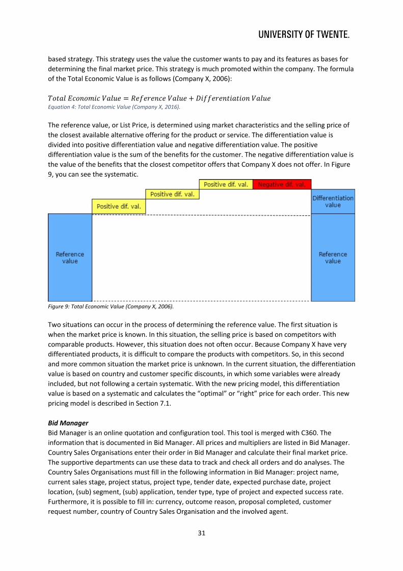
31
based strategy. This strategy uses the value the customer wants to pay and its features as bases for
determining the final market price. This strategy is much promoted within the company. The formula
of the Total Economic Value is as follows (Company X, 2006):
𝑇𝑜𝑡𝑎𝑙 𝐸𝑐𝑜𝑛𝑜𝑚𝑖𝑐 𝑉𝑎𝑙𝑢𝑒 = 𝑅𝑒𝑓𝑒𝑟𝑒𝑛𝑐𝑒 𝑉𝑎𝑙𝑢𝑒 + 𝐷𝑖𝑓𝑓𝑒𝑟𝑒𝑛𝑡𝑖𝑎𝑡𝑖𝑜𝑛 𝑉𝑎𝑙𝑢𝑒 Equation 4: Total Economic Value (Company X, 2016).
The reference value, or List Price, is determined using market characteristics and the selling price of
the closest available alternative offering for the product or service. The differentiation value is
divided into positive differentiation value and negative differentiation value. The positive
differentiation value is the sum of the benefits for the customer. The negative differentiation value is
the value of the benefits that the closest competitor offers that Company X does not offer. In Figure
9, you can see the systematic.
Figure 9: Total Economic Value (Company X, 2006).
Two situations can occur in the process of determining the reference value. The first situation is
when the market price is known. In this situation, the selling price is based on competitors with
comparable products. However, this situation does not often occur. Because Company X have very
differentiated products, it is difficult to compare the products with competitors. So, in this second
and more common situation the market price is unknown. In the current situation, the differentiation
value is based on country and customer specific discounts, in which some variables were already
included, but not following a certain systematic. With the new pricing model, this differentiation
value is based on a systematic and calculates the “optimal” or “right” price for each order. This new
pricing model is described in Section 7.1.
Bid Manager
Bid Manager is an online quotation and configuration tool. This tool is merged with C360. The
information that is documented in Bid Manager. All prices and multipliers are listed in Bid Manager.
Country Sales Organisations enter their order in Bid Manager and calculate their final market price.
The supportive departments can use these data to track and check all orders and do analyses. The
Country Sales Organisations must fill in the following information in Bid Manager: project name,
current sales stage, project status, project type, tender date, expected purchase date, project
location, (sub) segment, (sub) application, tender type, type of project and expected success rate.
Furthermore, it is possible to fill in: currency, outcome reason, proposal completed, customer
request number, country of Country Sales Organisation and the involved agent.

32
When all information is filled in, the orders are converted into a list with an overview of all projects.
After that, all project information is converted into a code. The List Price is retrieved from Company
X’s database and the selling price is calculated automatically. The supportive departments (Business
Development and Product Management) check these multipliers and adjust if the multiplier is too
low or too high. If the multiplier is lower than the Minimal Multiplier, the Country Sales Organisation
must ask permission of the supportive departments whether they can continue with their calculated
List Multiplier.
In Bid Manager, the List Price is divided into four categories. These four categories are: standard
product (switchgear), special materials for non-standard engineering, accessories and other (mostly
pack and transport cost). It is striking that for many orders the List Multiplier is only used for the first
category (the standard product or switchgear). The other three categories are in almost all cases
multiplied with 1.0. When we start with calculating the volumes in US Dollars, we use the same
method.
C360
C360 gathers information and status of every customer or project. This tool is merged with Bid
Manager, therefore the employees who work with one of these tools can change the data in the
other tool. Within C360, specific data of customer and project are stored. Examples are country, type
of product, special requirements, List Price, and List Multiplier. Furthermore, an estimated chance
that the order is continued is kept up. When the order is converted to C360, all actions are
documented and if the customer does not go along with Company X, the reason why is kept up. The
reason why the customer does not go along, is very important in this research. The lost orders due to
price, competitor or relationship, should be won now because the new model calculates the “right”
selling price.
When Country Sales Organisations convert the Bid Manager file to C360 the following fields must be
filled in: project name, sales stage, project type, tender date, expected purchase date, customer
name, segment (sales vertical), application, sub application and confidence percentage. Besides
these obligatory information, there are also fields that are not obligatory. These fields are: outcome
(won, lost or abandoned), currency, Country Sales Organisation, agent, tender version, project
location, end-use segment and project type. If not, all obligatory information is entered in Bid
Manager, the person who enters it, receives the message that required data are missing. Only after
the required information is filled in, the order information can be converted to C360. This could lead
to the fact that sales person guesses the required information to convert the information, which
leads to inaccurate data. Furthermore, not all variables of the new pricing model are (obligatory)
inputs in to convert to C360. To successfully implement and measure the new model, these variables
must be added and made obligatory to convert to C360. I come back to these two points in the
recommendations.
Two important limitations came forward in the interview with Employee Z (specialist in C360). The
first limitation was the fact that the data are not always documented properly because of slackness,
lack of personal interest or incomplete and unknown data. A second limitation that came forward,
was the fact that some orders are entered late in the sales process. The main reason for this, is that
the sales persons do not have to guess information, which is not known yet or because of laziness of
the sales persons. Furthermore, whether an order has less potential, the sales persons do not enter

33
the information, because the plant would know that they are working on a low potential order and
could be marked as time waste. This comes forward in the entered confidence levels of both
products in C360. This confidence level is the chance of success of a specific project. This is
respectively: X% and X% for Product 1 and Product 2. These are relatively high percentages
compared to the current hit-rates. Therefore, we conclude that the projects are entered late in C360.
Because of this, the performance measurements are not entirely accurate.
6.3 In which way are the price performances measured? In this section, we describe the price measuring tool of Company X.
Price measuring tool
Company X uses the Realized Price Index to measure the current performance against a period
average (Employee Z, 2016). The tool measures on a higher aggregated level and similar product
ranges. The tool uses historical data (from Bid Manager and C360) to measure the price changes. The
measurement is done monthly. However, the outcomes of the RPI-model are not used by the
management. Although this model is very useful to ground, pricing targets for specific markets or
products.
The RPI is calculated with the published price index (PPI) value, the List Multiplier, the constant price
(price at start of measuring) and the obtained price (price of won order)( Employee Z, 2016). To
calculate the RPI, all numbers in the equations must be known.
The RPI-values are calculated using two formulas(Employee Z, 2016):
𝑅𝑃𝐼 = 𝑃𝑃𝐼 ∗ 𝐿𝑖𝑠𝑡 𝑀𝑢𝑙𝑡𝑖𝑝𝑙𝑖𝑒𝑟 , where 𝐿𝑖𝑠𝑡 𝑀𝑢𝑙𝑡𝑖𝑝𝑙𝑖𝑒𝑟 =𝑂𝑏𝑡𝑎𝑖𝑛𝑒𝑑 𝑝𝑟𝑖𝑐𝑒
𝐿𝑖𝑠𝑡 𝑝𝑟𝑖𝑐𝑒
and 𝑃𝑃𝐼(𝑛𝑒𝑤) = (1 +𝐿𝑖𝑠𝑡 𝐶ℎ𝑎𝑛𝑔𝑒 (%)
100) ∗ 𝑃𝑃𝐼(𝑜𝑙𝑑)
𝑅𝑃𝐼 =𝑂𝑏𝑡𝑎𝑖𝑛𝑒𝑑 𝑝𝑟𝑖𝑐𝑒
𝐶𝑜𝑛𝑠𝑡𝑎𝑛𝑡 𝑝𝑟𝑖𝑐𝑒 , where Obtained price= Price of won order
Constant price= Price at start of measuring (2010)
𝐶𝑜𝑛𝑠𝑡𝑎𝑛𝑡 𝑝𝑟𝑖𝑐𝑒 =𝐿𝑖𝑠𝑡 𝑝𝑟𝑖𝑐𝑒
𝑃𝑃𝐼
Equation 5: RPI calculations (Employee Z, 2016).
It is also possible to calculate a combined RPI (this can be used for a product family) (Employee Z,
2016):
𝐶𝑜𝑚𝑏𝑖𝑛𝑒𝑑 𝑅𝑃𝐼 =𝑂𝑏𝑡𝑎𝑖𝑛𝑒𝑑 𝑝𝑟𝑖𝑐𝑒 (𝑝𝑟𝑜𝑑𝑢𝑐𝑡 1) + ⋯ + 𝑂𝑏𝑡𝑎𝑖𝑛𝑒𝑑 𝑃𝑟𝑖𝑐𝑒 (𝑝𝑟𝑜𝑑𝑢𝑐𝑡 𝑁)
𝐶𝑜𝑛𝑠𝑡𝑎𝑛𝑡 𝑝𝑟𝑖𝑐𝑒 (𝑝𝑟𝑜𝑑𝑢𝑐𝑡 1) + ⋯ + 𝐶𝑜𝑛𝑠𝑡𝑎𝑛𝑡 𝑝𝑟𝑖𝑐𝑒 (𝑝𝑟𝑜𝑑𝑢𝑐𝑡 𝑁)
Equation 6: Combined RPI calculation (Employee Z, 2016).
In the RPI-calculations, there are a couple limitations and points of attention to be considered
(Employee Z, 2016):
• If you raise the list price, the PPI must increase with the same percentage to get an accurate
RPI calculation. Otherwise an inverse relationship between the PPI value and RPI-value will
exist.
• Because the data in C360 and Bid Manager are not used consistently for trade pricing, the
accuracy of the RPI is not always reliable.

34
• Not many employees are familiar with this tool or use the outcomes of this tool, therefore
this tool is not always used or correctly used.
The new pricing model calculates for every order a List Multiplier, which changes the RPI-values. In
Section 8.1, we look at whether it is feasible to implement the variable List Multiplier in the RPI-
measurements and to which extent the RPI-values will change for Product 1 and Product 2.
6.4 What are the current financial performances? In this chapter, we evaluate the current (financial) performances of the Product Family X. It is
important to understand the current financial performances, to evaluate the financial impact.
Without the current situation, the new financial performances after implementation, cannot be
compared and the improvements are more difficult to measure. Besides the financial performances
also other relevant information are handled in this section. At the end of this chapter, we compare
the List Multiplier of four won projects with the new List Multiplier. This section gives us an idea of
what the exact impact on the selling price is and to which extent this differs to the won List
Multiplier.
6.4.1 Contracts vs projects In this assignment, we focus on projects, because contracts have only one moment of quotation for
mostly multiple deliveries. Therefore, the contracts are filtered and excluded in further calculations.
For this analysis, we use the report of Employee S (2017), in which for many countries the percentage
of public and private customers are calculated. Countries with large net sales ($) are also the ones
with the highest percentages of public customers. In a meeting with employee X, we decided to set
this percentage equal to the contract’s percentage for each country. In Table 7, the percentages
(%public/%private) for the concerning countries are shown (Employee S, 2017).
<CONFIDENTIAL TABLE> Table 7: Contracts vs. projects per country.
* Unfortunately, not all percentages are handled in the research of Employee S (2017). Therefore,
the countries with no percentage are considered 0/100.
6.4.2 Results and reasons lost, won or abandoned according to C360 In this section, we discuss the results of the analyses with the data of C360. Before starting the
analyses, the big contractors are excluded. Examples of big contractors of Company X are: Customer
X, Customer Y, and Customer Z (Employee S, 2017). In this way, the aim is more at the results of
projects, resulting in more reliable percentages. After the filtering, we look at the distribution of the
won, lost or abandoned revenue to determine the volume. This is evaluated in C360 because in this
tool, the outcome and reason why, are stored for each entered order.
In the table below we can see the percentages of projects that are won, lost or abandoned. These
data are retrieved from the data gathering tool: C360. According to Employee W (C360) not all data
are valid because carelessness of the filler or because the fact the data are not known. For the
Product 1 X orders and for the Product 2 X orders are analysed.

35
<CONFIDENTIAL FIGURE> Figure 10: Results Product 1 and Product 2.
In the graphs below the reasons why a deal is lost, won or abandoned is analysed.
<CONFIDENTIAL FIGURE> Figure 11: Reasons won, lost or abandoned for Product 1 and Product 2.
From both lost figures, we conclude that Company X lost many projects because of Company X’s
price and smaller but still notable number of projects are lost because of product offering and
relationship. If we look at the deals won, Company X aims at the relationship with its customers.
Also, the involvement of Company X in the decision-making process is shown in the percentage of
won because of Company X’s solution. The company aims to start in an early phase with the
customer to discover the customer’s needs to come up with a product which meets all properties.
This is shown in the reasons why projects are won due to price, these were only X% and X% of the
total won projects. Won due to relationship is by far the highest, namely X% and X% of the total won
projects. Therefore, we conclude that Company X is not a price fighter and focus on customer
relationship.
6.4.3 Current hit-rate To calculate the current hit-rate according to C360, the won projects are divided by the total projects
each month for the period of 2015-2016. So, the ratio of successful projects is examined.
Furthermore, we calculated the current hit-rate based on volume. To calculate this hit-rate, the
intake of 2016 from C360 is compared with the total quotation value from Bid Manager and from
C360. We have chosen to calculate further with the intake of 2016, because this number presents the
amount of money that is won, without the consideration of delivery times and payment terms. So,
when the project is won, this amount of money is added immediately to the intake.
However, the validity of the two data sources should be criticised. C360 is the most reliable source
for the won projects, because often only the quotations with high potential are entered in C360. The
most reliable source for the total quoted volume is determined by looking at the number of orders
that are entered in C360. Some countries have to few orders to do a good analyse. Therefore, we
consider C360 for the total quoted volume, if there is met to the minimal number of orders (the
priority rule). Otherwise, the quoted volume of Bid Manager is used for further calculations. The
drawback of Bid Manager is that quotations are sometimes entered multiple times or are just used as
an indication.
Together with my principal, we decided which hit-rate is most likely and created the priority rule. For
the countries in which C360 was often used, the C360 outcomes are taken seriously. When too few
orders have been entered in C360, the quotation volume of Bid Manager is taken. Only for Country
17 the outcome was extremely high and unlikely (X%). Therefore, no further calculations are done
with this hit-rate of Country 17.

36
Hit-rate with outcomes C360
Firstly, we discuss the calculations using only C360. The number of won projects is compared to the
number of lost or abandoned projects for each month, from January 2015 until December 2016. This
time range has been chosen because C360 was not fully operational at Company X before 2015. As
already mentioned in the theoretical perspective the hit-rate is the ratio of awarded projects. The
number of orders is listed in the table below for each month starting on January 2015 to December
2016. In the graphs below you can see that some hit-rates are 100% or 0%. In these months, mostly a
few orders are placed and therefore all orders in these months are successful (100%) or not
successful (0%). The average hit-rate is X% and X%, respectively for the Product 1 and Product 2,
according to C360.
<CONFIDENTIAL TABLE> Table 8:Number of entered quotations Product 1 & Product 2 2015-2016.
<CONFIDENTIAL FIGURE> Figure 12: Hit-rate 2015-2016 Product 1 (C360).
<CONFIDENTIAL FIGURE> Figure 13: Hit-rate 2015-2016 Product 2(C360).
In the graphs above, the average hit-rate is relatively high. This is because low potential orders are
not always converted from Bid Manager to C360, because these are considered as a waste of time.
Order volume hit-rate using intake and total quotation volume
Another way to calculate the hit-rate is by involving Bid Manager. This calculation is done by dividing
the intake of 2016 with the quoted volume of Bid Manager and C360. The projects do not have to be
filtered in these analyses, because no contracts are concluded. Because of the two different sources,
also two different hit-rates are calculated. This a very different calculation from the calculation as be
done in the previous paragraph. In this calculation, the focus is on the volume of the projects instead
of the number of projects that are won, lost or abandoned. The bold hit-rate percentages are the
percentages that represent best the actual hit-rates. In the rest of this report, these hit-rates are
named as most-likely hit-rate. The priority rule to choose the most-likely hit-rate is explained in
Section 7.2.
<CONFIDENTIAL TABLE> Table 9: Hit-rate Bid Manager.
6.4.4 Sales turnover In this section, we present the sales turnovers of both products. Firstly, we look at the volume of
orders won according to C360. Secondly, we look at the total sales turnover and intake per country
for 2016. The intake of 2016 per country is used in further calculations.
Sales turnover per month (C360)
In the graphs below, we present the revenues (sales turnover), retrieved from C360, for the Product
1 and Product 2 plotted for the 24 months of 2015 and 2016. In these graphs, we see that in the last
months of the year more revenue is achieved with several peaks. However, we must consider the
number of the projects. Not all information has been entered in 2015. In 2016 more projects have
been converted to C360 and this gives a better indication for the sales turnover.

37
<CONFIDENTIAL FIGURE> Figure 14: Revenues Product 1 2015-2016.
<CONFIDENTIAL FIGURE> Figure 15:Revenues Product 2 2015-2016.
In the graphs above, some peaks arise. This could mean that many or big projects have been offered
to Company X or many offers have been created. As already said in earlier sections, the data of C360
are not completely accurate. Not all orders have been entered in C360 and especially the volumes of
lost revenues and abandoned revenues should be much higher, because many projects are not
transferred from Bid Manager to C360.
Sales turnover and intake per country (C360)
In the table below the intake and sales turnovers are shown. Both are retrieved from C360. These
numbers are taken as base for the calculations for the most likely hit-rate, which is discussed in
Section 7.2.
<CONFIDENTIAL TABLE> Table 10: Sales turnover and intake 2016 (Employee W, 2017).
In Table 10, we miss the following countries: Country 10, Country 11, Country 12 and Country 15.
This means that no data were available for these countries. The sales have not been not filled in in
C360 or no sales have taken place at all. In further calculations, we continue with the intake (last
column), because this presents best the won volume. The sales turnover is the amount of money
received, after delivery times and payment terms. The intake gives us the sales when there is no time
between agreement and payment.
6.4.5 Segments The number of orders and the volume of each segment are investigated with two sources: C360 and
the report of Employee S (2017). This evaluation is useful to get a better insight in which segment
most projects are ordered to understand the impact per segment.
In Figure 16, the number of orders per segment are shown, retrieved from C360. Many projects are
entitled as unknown, other or unspecified and is a very large category compared to the known
segments. This is because many projects are filled in with carelessness or are set the wrong segment.
Therefore, many segments have zero projects. Because these data are not entirely valid, it cannot be
used in further calculations or an analyse per segment.

38
Figure 16: Orders per segment Product 1 and Product 2.
Besides the data of C360, also the report from Employee S (2017) is used to get a better
understanding of the distribution of the segments. The distribution is shown in Figure 17.
Figure 17: Breakdown by segment (Employee S, 2017).
These outcomes correspond to the outcomes of C360. Also, the utility, commercial and industries are
in this report the largest markets for Company X. Therefore, we conclude that Company X has the
largest sales in these segments.
6.4.6 Financial performances In this section, we discuss the current financial performance indicators, current standard,
manufacturing and operating profit. Furthermore, we explain the Transfer Multiplier.
Standard profit and margin
Firstly, we discuss the standard profit. As already mentioned in Section 4.1 the standard profit is the
sales turnover or revenue, minus the material cost and labour cost. The material cost is the cost for
the materials that are needed to manufacture the concerned product. The labour cost is calculated
by multiplying the necessary working hours by the salary per hour. In the current operations,
Company X aims to get a standard average margin of approximately Z% per order. This percentage is
119
200
232
15 4 0 0 0
191
132
0
50
100
150
200
250
Orders segments per segments Product 1 2015-
2016
57
160
197
271 0 0 0
36
81
0
50
100
150
200
250
Orders segments Product 2 2015-2016

39
chosen because with this percentage it is likely that there is an operating profit or end-to-end profit
at the end. We took the average List Price and average material- and labour cost. Therefore, the only
variable is the List Multiplier to calculate the standard profit of all countries.
𝑆𝑡𝑎𝑛𝑑𝑎𝑟𝑑 𝑝𝑟𝑜𝑓𝑖𝑡 𝑝𝑒𝑟 𝑝𝑟𝑜𝑑𝑢𝑐𝑡($) = 𝐿𝑖𝑠𝑡 𝑃𝑟𝑖𝑐𝑒 ∗ 𝐿𝑖𝑠𝑡 𝑀𝑢𝑙𝑡𝑖𝑝𝑙𝑖𝑒𝑟 − 𝑀𝑎𝑡𝑒𝑟𝑖𝑎𝑙 𝑐𝑜𝑠𝑡 − 𝐿𝑎𝑏𝑜𝑢𝑟 𝑐𝑜𝑠𝑡 Equation 7: Standard profit per product ($) (Company X, 2006).
If we fill this equation with the prices and cost for a standard Product 1 and Product 2(see Section
7.2) the Standard profit ($) and the necessary, List Multiplier to achieve Z% standard margin is as
follows:
• Product 1.
X * List Multiplier -Y.
Positive standard profit per product is achieved with a List Multiplier of Y/X=0.458. To achieve a Z%
standard profit (profit/sales), to cover manufacturing cost and operating cost, the List Multiplier
should be: X / (1-Z) / X= 0.705.
• Product 2.
x*List Multiplier-Y.
Positive standard profit per product is achieved with a List Multiplier of Y/X=0.433. To achieve a Z%
standard profit (profit/sales), to cover manufacturing cost and operating cost, the List Multiplier
should be: Y / (1-Z) / X=0.666.
To calculate the current profit margins, the Product Line X May 2017 YTD document is used
(Company X, 2017). The current overall standard margin is X%. In US Dollars, this means: $X standard
profit. The total overview and calculations of all current margins are listed in Appendix 1, in the
column named: “2017 Profit Plan”.
Current manufacturing profit and margin
The manufacturing profit is calculated by subtracting the manufacturing cost (or net variance cost)
from the standard profit. Because not all data have been stored of these cost per country, the overall
manufacturing cost per product of Company X is used, retrieved from the YTD Actuals of May 2017.
The overall manufacturing cost per product is X%-X%=X% of total sales (Company X, 2017). In US
Dollars, this means: $X manufacturing cost. The current overall manufacturing profit is $X and the
manufacturing margin is X% of total sales (Company X, 2017).
𝑀𝑎𝑛𝑢𝑓𝑎𝑐𝑡𝑢𝑟𝑖𝑛𝑔 𝑝𝑟𝑜𝑓𝑖𝑡($) = 𝑆𝑡𝑎𝑛𝑑𝑎𝑟𝑑 𝑝𝑟𝑜𝑓𝑖𝑡($) − 𝑀𝑎𝑛𝑢𝑓𝑎𝑐𝑡𝑢𝑟𝑖𝑛𝑔 𝑐𝑜𝑠𝑡($) Equation 8: Manufacturing profit.
Current operating profit and margin
Just as the manufacturing profit, the average of supportive cost per product of Company X is used,
resulting from the YTD Actuals of May 2017. The average operating cost for the Product Line X is X%
of total sales (Company X, 2017). In US Dollars, this means: $ X operating cost. The current operating
profit is $X and the operating margin is X% of total sales (Company X, 2017).
𝑂𝑝𝑒𝑟𝑎𝑡𝑖𝑛𝑔 𝑝𝑟𝑜𝑓𝑖𝑡($) = 𝑀𝑎𝑛𝑢𝑓𝑎𝑐𝑢𝑡𝑢𝑟𝑖𝑛𝑔 𝑝𝑟𝑜𝑓𝑖𝑡($) − 𝐷𝑖𝑠𝑡𝑟𝑖𝑏𝑢𝑡𝑖𝑜𝑛 𝑐𝑜𝑠𝑡($) −
𝐴𝑑𝑚𝑖𝑛𝑖𝑠𝑡𝑟𝑎𝑡𝑖𝑣𝑒 𝑐𝑜𝑠𝑡($) − 𝑆𝑒𝑙𝑙𝑖𝑛𝑔 𝑐𝑜𝑠𝑡($) − 𝑅&𝐷 𝑐𝑜𝑠𝑡($) − 𝑜𝑡ℎ𝑒𝑟 𝑐𝑜𝑠𝑡($) + 𝑜𝑡ℎ𝑒𝑟 𝑖𝑛𝑐𝑜𝑚𝑒($) Equation 9: Operating profit.

40
Link with transfer multiplier
The supportive cost caused by the wages of the supportive employees (wages), wages of the
employees of Country Sales Organisations and bonusses for the Country Sales Organisations, which
are different for each order and product (variable cost). For standard projects or contracts a fixed
percentage is taken to pay the Country Sales Organisations. When it is a special, mostly with more
volume, the Country Sales Organisations are payed with X percent of the total sales volume, which is
called Commit. Unfortunately, not all product lines are following this systematic, especially the
Product Line X (including Product 1 and Product 2). These products have their own calculation of
what the Country Sales Organisation can keep as their wage. For these products, the difference
between the Transfer Multiplier and the achieved List Multiplier is payment for the Country Sales
Organisations. So, the Transfer Multiplier is the purchase price for Company X’s Country Sales
Organisation. These Transfer Multipliers are mostly around X. For example, when a Country Sales
Organisation won a project with a List Multiplier of X with a Transfer Multiplier of X, the Country
Sales Organisation keep X percent of the total sales turnover. With these revenues, the Country Sales
Organisation can pay the wages and all other variable and fixed cost. On top of that, it was agreed
within Company X that each Country Sales Organisation should make approximately X percent profit
margin. The overview of all Transfer Multipliers is listed below. Country 7 and Country 15 have no
own Transfer Multiplier. This is because the sales for Country 7 are directly from Company X, and
Country 15 uses the same Transfer Multiplier as Country 5.
<CONFIDENTIAL TABLE> Table 11: Transfer Multipliers.
Every country has different Transfer Multiplier because every country has their own market
characteristics and own customer’s willingness to pay. The Transfer Multipliers are reviewed and
adapted if necessary, every year by the financial and pricing departments.
6.4.7 Comparison won orders Finally, we evaluate some won orders in the past. In this section, we compare the List Multiplier, with
which the order is won and the List Multiplier following the new pricing model of Edens (2016).
Furthermore, the difference in sales is calculated using the New Multiplier. The information to fill in
all variables are obtained with employee U (Manager Business Support Commercial and Large
Projects), employee Y (Manager Product Marketing Bid Manager) and Employee R (Manager Business
Development Segments). These data are used to fill in the variables as stated by Edens (2016). Four
recent orders are evaluated. These four have been selected because these contain a Product 1 or
Product 2 order. Many orders were not included because the order was maintenance or partial
renewal. In the tables below the plural comparison is made. Because there is also a different List
Multiplier used for the accessories and others, we used 1.000 for this category. The calculated List
Multiplier is used for the List Price of the Product 1 Switchgear.
<CONFIDENTIAL TABLE> Table 12: Data four won projects/contracts.
<CONFIDENTIAL TABLE> Table 13: Calculation new multiplier & difference in sales for four won projects/contracts.

41
In Table 12 the choices for every variable are shown, resulting in a new List Multiplier. This new List
Multiplier is shown in the first column of Table 13. In the second and third column of Table 13, the
List Multiplier is shown for which the order is won. As can be seen, the difference for the larger
project or long contract is not very big (<10%). Therefore, we see no big implications for these two
orders. For the small orders, there is a greater difference. Especially for SSE contracting, in which
Eaton could miss almost three thousand US Dollars. Therefore, it is wise to check and analyse the
orders with a large volume. In the recommendations, I come back to this. Four comparisons are too
low to draw conclusions. Therefore, these comparisons should be extended in further research. With
more comparisons, Eaton can test the new pricing model and link this with this assignment.
7. Financial impact of new pricing model In this chapter, we evaluate the financial impact of the new pricing model (Edens, 2016). Firstly, we
describe the variables of the new pricing model and in which way they calculate the “right” price.
Secondly, we evaluate the margin changes. So, we compare the old margins (operating and standard
margin) with the margins using the new pricing model. Thirdly, we give an estimation of the sales
volume changes because of the new pricing model. All these outcomes are calculated using an Excel
document. The assumptions and methods are described in concerning sections. Many outcomes are
listed within this chapter. Summary sheets of all calculations and the Product Line statement are
placed in Appendix 1. Finally, we look at other performances rates that changes because of the new
pricing model. In this sub-question, we look for example at the change in RPI-value. The main
question together with the sub-questions are listed below.
Which performances are affected by the new pricing model and what is the expected impact on these performances? This main question is divided into the following sub-questions:
• What are the new variables and in which way do they calculate the “right” selling price?
• What are the expected profit and demand changes?
• Which other important performances change because of the new pricing model?
7.1 What are the new variables and in which way do they calculate the “right” selling
price? In this research, we must understand the bachelor assignment of Edens (2016) to gain a better
understanding the modifications and the (financial) impact. Currently the selling price is determined
with country and customer related discounts. Edens (2016) determines the price based on seven
variables. These variables and the table with weights and score ranges are listed below.

42
Variable (i) Explanation
1. Position Five different scales for classifying the countries. The countries are classified using SF6 free, which is based on the Climate Change Performance Index. This index considers: emission level, development of emissions and climate policy. The better the country scores on this index, the higher the score for this variable.
2. Country Customer’s country of residence score based on purchasing power, surveys and a benchmark score. The higher these aspects, the higher the score for this variable.
3. Customer relationship
Four different states of customer relation: Long relationship (>5 deals in the past), short relationship (1-5 deals in the past), rejected (contracted but no deals in the past) and first contract (no contact in the past). The more contacts in the past, the higher score for this variable.
4. Volume Five different volumes. Small project (<$20000), medium project ($20000-$50000), large project (>$50000), short contract and long contract. The smaller or shorter the project or contract, the higher the score for this variable.
5. Segment Ten different market segments of customers. Because the average prices differ in different markets, key account managers and business development managers are asked to rank the segments. Fifth and sixth are the reference points and the upward or downward step size is 2,5%.
6. Sales process Moment of customer contract. The phase in which the customer enters the sales stages, the higher the score for this variable.
7. Competitors Number of competitors in the market in a certain area. This has five different states, namely: 0 competitors, 1 competitor, 2 competitors, 3-4 competitors and 5 or more competitors. The higher the number of competitors present in the market, the lower the score of this variable.
Table 14 New variables (Edens, 2016).
Variable Weight (Wi) Score range(Si)
1. Position - [0.00-0.07]
2. Country - [-0.08-0.08]
3. Customer relationship 0.349 [0.80-1.15]
4. Volume 0.156 [0.80-1.15]
5. Segment 0.068 [0.90-1.10]
6. Sales process 0.272 [0.80-1.15]
7. Competitors 0.156 [0.85-1.10] Table 15: Weights and Scores per variable.
Each variable received a weight (Wi) and score (Si), in which all customers can be assigned to a
specific multiplier (see table above). For the determination of the selling price, Company X first
determines a List Price for every product. This List Price is set for every product with every type of
addition to the standard product. When new features are added for a certain product, a new List
Price is created considering the material, development and labour cost. According to Employee R
(manager business development), this List Price is based on market prices of competitors and
experience. The final market price for the Product Family X is calculated according to the following
formulas (Edens, 2016):
𝐹𝑖𝑛𝑎𝑙 𝑚𝑎𝑟𝑘𝑒𝑡 𝑝𝑟𝑖𝑐𝑒 = 𝐿𝑖𝑠𝑡 𝑝𝑟𝑖𝑐𝑒 ∗ (0.735 + 𝐷𝑖𝑓𝑓𝑒𝑟𝑒𝑛𝑡𝑖𝑎𝑡𝑖𝑜𝑛 𝑣𝑎𝑙𝑢𝑒) Equation 10 Final market price.
𝐷𝑖𝑓𝑓𝑒𝑟𝑒𝑛𝑡𝑖𝑎𝑡𝑖𝑜𝑛 𝑣𝑎𝑙𝑢𝑒 = 𝑆1 + 𝑆2 − (1 − (𝑊3 ∗ 𝑆3 + 𝑊4 ∗ 𝑆4 + 𝑊5 ∗ 𝑆5 + 𝑊6 ∗ 𝑆6 + 𝑊7 ∗ 𝑆7) Equation 11: Differentiation value.

43
With this new way of calculating the differentiation value, the pricing policy is more variable and
customised for each customer. The final market price is restricted to 0.470 on the lower side and
1.000 on the upper side (Edens, 2016). With this variable way of pricing, we assume that a better first
offer is given to the customers and the objective to increase the operating profit can be pursued. But,
this assumption must be evaluated and tested further in this research.
7.2 What are the expected profit and demand changes? In this section, we estimate the possible financial impact of the new pricing model. To estimate the
impact, we do calculations on the following aspects to estimate the (expected) financial impact:
change in List Multiplier, change in hit-rate, change in sales turnover and change in profit margins.
These calculations are done using the program Excel. In this way, all calculations are linked to each
other. In the excel document, a summary sheet is created with all the main outcomes of all.
Furthermore, the input sheets (labelled with a green colour), can be adapted by Company X, when
better data are available. This makes it possible to use this model in the future.
7.2.1 Change in List Multiplier In this section, we discuss the current List Multipliers and the List Multipliers calculated with the new
pricing model. All these multipliers are plotted in the graphs further in this section. An explanation
and the source and method of these multipliers are explained below for every multiplier.
• Firstly, we discuss the worst-case and best-case multiplier for each country, when following
the new pricing model. The worst-case and best-case multipliers are calculated with the
country specific variable scores supplemented with all minimal or maximal scores for each
variable.
• Secondly, we discuss the current Minimal Multiplier. This multiplier is retrieved from the first
revision of the Multiplier Overview made on 1st February 2017. In the current situation, all
List Multipliers are defined per country. For every country, there is a target and minimal List
Multiplier. Country Sales Organisations can offer Company X’s product in this range (see
Section 6.1). Often the used List Multiplier is close to the Minimal Multiplier. This is because
the Target Multiplier is often not achievable. When the Country Sales Organisations only can
sell Company X’s products for a lower List Multiplier than the Minimum Multiplier, they
should ask permission to the supportive departments. The higher the volume, the higher
ranked employee who must give permission for the order.
• Thirdly, the quoted List Multiplier is retrieved from the RPI-calculations, which are retrieved
from Bid Manager. Because only the Product 1 is measured with the RPI-model, only the
quoted List Multiplier for the Product 1 is available. Therefore, this List Multiplier is excluded
in the graph of the Product 2. The quoted List Multiplier is calculated by taking the weighted
average of the period 2016-2017. Unfortunately, there were no data for the countries:
Country 15, Oman, Country 11, Country 12 and Country 16 in the chosen time interval. This
can have two meanings: no data have been entered in Bid Manager or there were no
successful deals in the time interval. For these countries, the Minimal Multiplier is taken. In a
conversation with Employee Z (Strategic Pricing Manager), these values are taken from the
last entered data for each order. Therefore, it cannot be said with 100% certainty that these
values are the locked and winning List Multiplier. The quoted List Multiplier is often near the
Minimal Multiplier.
• Fourthly, the new List Multiplier is calculated, according to the new pricing model. The new
List Multiplier is calculated by taking the country and position specific variable score,

44
multiplied by the weight for these two variables. For the other five variables, a different
approach is chosen. the most common outcome per variable per type of order (project or
contract) is chosen together with my principal. These outcomes for both projects and
contracts are filled in and multiplied with the weight of each variable. These outcomes are
summed for both projects and contracts. After that these outcomes are multiplied with the
distribution of contracts and projects in each country. This weighted average gives a good
direction for what the differentiation value is when implementing the new pricing model.
The outcomes of these five multipliers for each country can now be summarised in graphs. With
these graphs, we can seek for striking results and make several comparisons. The worst case, new
and best-case multipliers are the same for Product 1 and Product 2. However, the Minimal Multiplier
is different for some countries. Both graphs are shown below.
<CONFIDENTIAL FIGURE> Figure 18: Multiplier scenarios per country per product.
The first striking thing in these graphs are that the Minimal Multipliers of Country 1 and Country 2
are above the best-case List Multiplier. This means that, in the current situation the products in these
two countries are offered for a too high List Multiplier. Therefore, there is much potential in these
markets, when lowering the List Multiplier. All other Minimal Multipliers are within the bandwidth of
the worst case and best-case List Multiplier. Furthermore, for many countries the Minimal Multiplier
is above the new, calculated List Multiplier. This would mean that these countries can lower their
price. All changes in percentages are shown in Figure 19 and Figure 20.
Another striking point is that the average quoted List Multipliers for some countries are below the
Minimal Multiplier. This is remarkable because all the orders that are below the Minimal Multiplier
must be communicated to the plant in City X and for the big differences even to the Product Line
manager: employee X. Especially Country 3 is very remarkable. The quoted List Multiplier is 0.123
lower than the Minimal Multiplier. This would mean that for many order permissions should have
been asked from the supportive departments in City X.
<CONFIDENTIAL FIGURE> Figure 19: Difference minimal and calculated List Multipliers.
<CONFIDENTIAL FIGURE> Figure 20: Difference minimal and calculated List Multiplier (%).
From Figure 19 and Figure 20, we conclude that the new List Multipliers decrease for most countries.
Especially Country 1 and Country 2, which even decrease by X%. It should be said that these
countries had a very high List Multiplier, almost equal to the best-selling countries. Therefore, it is
not very strange that these two countries have almost no market shares.
7.2.2 Change in hit-rate In this section, we look at the change in the hit-rate. During the assignment, we concluded that it is
not possible to predict the ratio using the price elasticity of demand, because of the diversified
product with very diversified prices for each country and customer. Therefore, we have changed the
approach to calculate the hit-rate. We investigate the volume which is lost because of the variables

45
of the new pricing model. Not all countries have sales entered in Bid Manager and C360 in the period
2015-2016. Therefore, these countries are not considered further in the calculations and this
assignment. The countries for which this is the case are: Country 15, Oman, Country 11 and Country
12.
Data gathering with C360 and Bid Manager
In Section 6.4, we calculated the current hit-rate using the intake (revenues from all completed
projects) and quotation value from Bid Manager and C360. This calculation is more focused on the
volume of the orders instead of the amount of orders which are successful, compared to the number
of lost orders.
Intake 2016
To indicate the project volume per country we multiplied the intake of 2016 by the percentages of
projects per country, according to Employee S (2017). In this way, we investigate the volume of the
projects for each country. Contracts are excluded because they can have multiple payments, which
results in an inaccurate comparison, because the quoted volume could be in earlier periods and the
output in later periods. Even after the contracts exclusion still some unexpected results arise. This is
because not many orders have taken place (for example Country 4), have been entered incorrectly,
or have been entered twice. Therefore, the validity of these outcomes should be doubted. In the
recommendations, we come back to this to calculate the intakes, when more reliable intakes are
known.
Current most likely hit-rate and priority rule
For the quoted volumes of 2016 we consider Bid Manager and C360. For C360 the quoted volume of
2016 is calculated in two ways, namely using the data from total list of all orders and the data from
the document, from which the intake and profit plan are retrieved. For some countries, the volume
and number of orders were equal in these two documents but for most countries this was not the
case. Therefore, both documents are used and the document with most orders is considered as most
reliable. The reason why these documents are different is because the data are filtered on doubles,
contracts or other aspects. Because no contracts are quoted in C360 in 2016, the quoted volumes of
C360 do not have to be multiplied with the percentage of projects in the concerned country.
Together with my principal, we selected the most likely hit-rates for all 18 concerned countries,
choosing between the data from Bid Manager and C360. We developed a priority rule to choose the
most likely quoted volume, resulting in a most likely hit-rate. In addition, this priority rule is also used
whether the outcomes for percentage of lost due to price, competitor and relationship is reliable.
The data of C360 had the main priority when choosing the most likely hit-rate, despite some not
entered data (especially lost orders). If there were enough observations (orders), C360 is used as
source for the calculations. To do further calculations using the data of C360, we have chosen for a
minimal number of 9 orders per country for 2016. In this way, the top-selling and medium-selling
countries are calculated with the data of C360. When countries have less than 9 orders in 2016, we
considered the quoted volume of Bid Manager. After that, the most likely hit-rate is calculated by
dividing the intake 2016 (excl. contracts) with the selected quoted volume. We considered the most
likely hit-rate, if the hit-rate is below 50%. So, the won volume should be less than the half of the
quoted volume.

46
After this priority rule, for 17 of 18 countries a likable hit-rate is calculated. Only for Country 17 an
unlikeable hit-rate came forward, namely X%. Because no data was available in C360, the data from
Bid Manager must be taken. This would mean that Xpercent of all quoted volume is won by Company
X. This is very unlikely, which is also strengthened by the percentage that is lost on price, relationship
and competitor, according to the Country Sales Organisation (see Section 7.3). Therefore, we have
chosen to set this most likely hit-rate as invalid. The average hit-rate for Product 1, using the priority
rule is X%.
<CONFIDENTIAL TABLE> Table 16:Most likely hit-rate Product 1 2016.
For Product 2 it was more difficult to calculate the most likely hit-rates because of more
incompleteness of the data. The results are shown in the table below. Many countries have a most
likely hit-rate of 0%. This indicates that no successful projects took place in 2016 and converted to
C360. The average hit-rate for Product 2 using the priority rule is X%.
<CONFIDENTIAL TABLE> Table 17: Most likely hit-rate Product 2 2016.
Now we know the current hit-rates and the priority rule, we can compare these numbers to the
expectations for 2017 and 2018 using the new pricing model. This is elaborated below.
Growth potential
To predict the new hit-rates we take a closer look at the potential market shares and the part of the
lost orders due to price, relationship and competitor. Because of the extra intake, the market share
also increases. In the beginning, we assumed that all orders which are lost due to price, relationship
and competitor are won, when using the new calculated List Multiplier. This extra intake is summed
with the current market sales of Company X market and divided by the total market volume of the
Secondary Switchgears. Especially the three top-selling countries with a market share above X%,
should get extra attention, because these sales are very important for the profitability of Company X.
It is difficult to predict precisely the new intake, because of the assumptions that have been made
and many unknown side effects that play a role in winning an order.
Firstly, the percentage of lost orders due to price, relationship and competitors (P.R.C.) is
determined. These three variables are included in the new pricing model and should be won now.
The percentage is calculated by the number of projects that are lost due to P.R.C. divided by the total
projects. During the calculations with data of C360 in Chapter 6, we came to the conclusions that not
all data are available to calculate this percentage. Therefore, we have chosen to contact the Country
Sales Organisations, to ask what they estimate based on their experience. For each country, one
employee of the concerned country has been contacted. The findings of these contacts are listed
below. Not all sales persons give the percentages of both products. When only one percentage is
given, this percentage is used for both products.
<CONFIDENTIAL TABLE> Table 18: Lost due to price, relationship and competitor according to Country Sales Organisations.

47
In Table 18, we see that the percentages are very high in most countries. Therefore, we conclude
that there is much potential for all these countries. The outcomes of Country 1, Country 2 and
Country 5 are remarkable. Country 1 has no up-to-date data, because Company X is abandoning this
market and no new orders are taking place soon. Country 2 has just started with selling the products
of the Product Family X and therefore, the data are insufficient to give a good approximation.
Country 5 lose 0% on price, relationship and competitor. This is because the selling prices of the
Country 5 are argued as very fine tuned with the market. In a conversation with Employee Z, we
concluded that the outcomes of the above table do not perfectly represent the actual percentages.
These sales persons look from their sales perspective and could deviate from reality. Therefore, these
outcomes are only taken when the data of C360 are insufficient.
Secondly, the market share potential is evaluated. To calculate the market share increase, the intake
increase must be calculated. This increase should be added to the current market sales of Company
X. For these calculations, we use multiple sources, both internal as external. The potential is
calculated by looking at the current market share per country, current market sales of Company X
per country, total market volume per country (Company X, 2017), Intake of 2016 (C360), quotation
volume from Bid Manager, quotation volume from C360 and percentage of which amount of orders
are lost due to price, relationship and competitor (C360 & survey with Country Sales Organisations).
The current market share is the current market share on the market of secondary switchgears.
Besides the Product Family X, also more products are included in this market sales, but these
products are not in the scope of this assignment. Because the markets sales are not separated per
product, we use the market sales of this market sales as base and add the potential extra intake from
the Product Family X.
As mentioned earlier, the data from Bid Manager and C360 are not entirely accurate. In Bid Manager,
some orders are placed multiple times to check or because of other reasons, after which not all
double orders have been removed and remained in the Bid Manager data. Together with employee
Y, we have chosen to multiply the total quoted volume with a correction factor of 0.8 to calculate a
more reliable quoted volume. The quoted volume of C360 is also not entirely reliable because not all
orders are transferred from Bid Manager to C360. However, the orders that are transferred to C360,
are considered as reliable.
Besides the calculations of C360 (lost because of P.R.C.) with C360 (quoted volume) and survey
(C.S.O.) with Bid Manager (quoted volume), also a hybrid is created and calculated. For this hybrid,
the same priority rule is used as for the most likely hit-rate. Therefore, firstly the number of orders of
C360 is analysed. If the number of orders is more than 9 orders, the data from C360 are used.
Otherwise the survey and the quoted volume of Bid Manager is used. The sales persons give their
expectations on the total lost orders. To calculate the potential extra intake, this percentage must be
corrected to a percentage on the total orders (see second possibility in Equation 12). Concluding the
following formulas are used to calculate the intake increase and market volume increase:
1. 𝑃𝑜𝑡𝑒𝑛𝑡𝑖𝑎𝑙 𝑒𝑥𝑡𝑟𝑎 𝑖𝑛𝑡𝑎𝑘𝑒(𝑢𝑠𝑖𝑛𝑔 𝐶360 𝑝𝑒𝑟 𝑐𝑜𝑢𝑛𝑡𝑟𝑦) = 𝐿𝑜𝑠𝑡 𝑑𝑢𝑒 𝑃. 𝑅. 𝐶. (𝐶360) ∗
𝑇𝑜𝑡𝑎𝑙 𝑞𝑢𝑜𝑡𝑒𝑑 𝑣𝑜𝑙𝑢𝑚𝑒 (𝐶360)
2. 𝑃𝑜𝑡𝑒𝑛𝑡𝑖𝑎𝑙 𝑒𝑥𝑡𝑟𝑎 𝑖𝑛𝑡𝑎𝑘𝑒(𝑢𝑠𝑖𝑛𝑔 𝐵𝑖𝑑 𝑀𝑎𝑛𝑎𝑔𝑒𝑟 𝑎𝑛𝑑 𝑠𝑢𝑟𝑣𝑒𝑦) =
𝐿𝑜𝑠𝑡 𝑑𝑢𝑒 𝑃. 𝑅. 𝐶. (𝑠𝑢𝑟𝑣𝑒𝑦) ∗ 𝑇𝑜𝑡𝑎𝑙 𝑞𝑢𝑜𝑡𝑒𝑑 𝑣𝑜𝑙𝑢𝑚𝑒 (𝐵𝑖𝑑 𝑀𝑎𝑛𝑎𝑔𝑒𝑟)
3. 𝑃𝑜𝑡𝑒𝑛𝑡𝑖𝑎𝑙 𝑒𝑥𝑡𝑟𝑎 𝑖𝑛𝑡𝑎𝑘𝑒(ℎ𝑦𝑏𝑟𝑖𝑑) = 𝐿𝑜𝑠𝑡 𝑑𝑢𝑒 𝑃. 𝑅. 𝐶. (𝐻𝑦𝑏𝑟𝑖𝑑) ∗
𝑇𝑜𝑡𝑎𝑙 𝑞𝑢𝑜𝑡𝑒𝑑 𝑣𝑜𝑙𝑢𝑚𝑒(𝐻𝑦𝑏𝑟𝑖𝑑) Equation 12: Potential extra intake (three possibilities).

48
𝑃𝑜𝑡𝑒𝑛𝑡𝑖𝑎𝑙 𝑚𝑎𝑟𝑘𝑒𝑡 𝑠ℎ𝑎𝑟𝑒 =𝐶𝑢𝑟𝑟𝑒𝑛𝑡 𝑚𝑎𝑟𝑘𝑒𝑡 𝑠𝑎𝑙𝑒𝑠 + (𝑛𝑒𝑤 𝑝𝑜𝑡𝑒𝑛𝑡𝑖𝑎𝑙 𝑚𝑎𝑟𝑘𝑒𝑡 𝑠𝑎𝑙𝑒𝑠 − 𝑖𝑛𝑡𝑎𝑘𝑒 2016)
𝑇𝑜𝑡𝑎𝑙 𝑚𝑎𝑟𝑘𝑒𝑡 𝑣𝑜𝑙𝑢𝑚𝑒
Equation 13: Potential market share.
The current market share and the market share increases for all 18 researched countries with the
new intake of Product 1 are shown in the table below.\
<CONFIDENTIAL TABLE> Table 19: Potential market share increase with new intake Product 1 and Product 2.
According to employee X, it is unrealistic that the top-selling countries (Country 8, Country 7 and
Country 6) increase much. Maintaining the sales in these markets should be the main priority.
Therefore, the top selling countries should get more attention, to avoid a lowering of the overall
profitability. In the worst case, the current sales and market share decrease, because regular
customers abandon Company X. To avoid such situation, I advise to have more supervision on the
larger projects and contracts (>$ 50,000) of the Product Line and Business Development department
in City X. In this way, the profitability is more protected and improved, if possible. I come back to this
in the recommendations.
Calculation potential hit-rate
To calculate the potential hit-rate, we formulated an equation. Because the assumption is made, that
the new List Multiplier results in the “right” price, the orders that are lost due to P.R.C. are now won.
Therefore, this percentage is added to the current most likely hit-rate. The hybrid percentage is taken
because this is considered as the most reliable increase.
𝑃𝑜𝑡𝑒𝑛𝑡𝑖𝑎𝑙 𝑛𝑒𝑤 ℎ𝑖𝑡 − 𝑟𝑎𝑡𝑒 (%) = 𝑀𝑜𝑠𝑡 𝑙𝑖𝑘𝑒𝑙𝑦 ℎ𝑖𝑡 − 𝑟𝑎𝑡𝑒 2016 (%) + 𝐿𝑜𝑠𝑡 𝑑𝑢𝑒 𝑃. 𝑅. 𝐶. (ℎ𝑦𝑏𝑟𝑖𝑑) Equation 14: Potential new hit-rate.
The outcomes of the potential hit-rates for Product 1 are shown in Table 20.
<CONFIDENTIAL TABLE> Table 20: Calculated potential new hit-rate Product 1.
With the findings of Table 20, we see that there is potential in most of the markets when the orders
which are lost due to price, relationship and competitor are won. The higher the percentage lost due
to price, competitor and relationship, the higher the potential extra intake, given the total quoted
volume. Some countries have very high potential hit-rates, Country 6 even above 100%. This is
because all orders that are lost due to P.R.C. are added to current situation. Whether all these lost
orders will be won, should be proven in practice. For Country 6, the current intake of 2016 summed
with the potential intake is more than the total quoted volume of 2016. Therefore, we see again that
the data are not entirely accurate.
In Table 21, the same method is used to calculate the potential new hit-rate for Product 2.
<CONFIDENTIAL TABLE> Table 21:Calculated potential new hit-rate Product 2.

49
Just as the outcomes for Product 1, the potential hit-rates of Product 2 increase much. Furthermore,
Product 2 has just been launched in many countries. This can also be seen in the current most likely
hit-rates, which are zero for seven countries and are below 1 percent for many.
7.2.3 Change in sales turnover In the previous section, we already calculated the potential extra intake, to calculate the potential
market share. In this section, we calculate the new potential intake. The change in sales turnover is
very important to measure the success of the new pricing model. We chose to calculate with the
outcomes of the hybrid formula, because this formula considers the number of observations (orders)
in C360, to calculate with a more reliable quoted volume. The potential intake volume is calculated
using the following formula:
𝑃𝑜𝑡𝑒𝑛𝑡𝑖𝑎𝑙 𝑖𝑛𝑡𝑎𝑘𝑒 𝑣𝑜𝑙𝑢𝑚𝑒 (ℎ𝑦𝑏𝑟𝑖𝑑)= 𝐶𝑢𝑟𝑟𝑒𝑛𝑡 𝑖𝑛𝑡𝑎𝑘𝑒 2016 (𝑖𝑛𝑐𝑙𝑢𝑑𝑖𝑛𝑔 𝑐𝑜𝑛𝑡𝑟𝑎𝑐𝑡𝑠) +
(𝐿𝑜𝑠𝑡 𝑑𝑢𝑒 𝑃. 𝑅. 𝐶. (ℎ𝑦𝑏𝑟𝑖𝑑) ∗ 𝑇𝑜𝑡𝑎𝑙 𝑄𝑢𝑜𝑡𝑒𝑑 𝑣𝑜𝑙𝑢𝑚𝑒 (ℎ𝑦𝑏𝑟𝑖𝑑)) Equation 15:Potential intake volume.
Using the formula above for hybrid, the outcomes per product and per country are calculated and
shown in Table 22 and Table 23.
<CONFIDENTIAL TABLE> Table 22: New intake Product 1.
<CONFIDENTIAL TABLE> Table 23: New intake Product 2.
In the calculated (ideal) situation the intake volume of Product 1 goes from $X to $X. So, an increase
of $X extra intake volume for the Product 1. For Product 2 the intake volume increases with $ X to $
X.
Not all data are 100 percent watertight, therefore we looked whether the increase is realistic. As
already mentioned in the section of the market shares, Country 6, Country 7 and Country 8 have
large market shares and are very important for the profitability of Company X. Therefore, large
projects and contract should get extra attention, at the beginning. In this way, the profitability is
more protected and the risks are lower. In the recommendations, we come back to this.
An extra calculation has been made without the three top-selling countries. In this case the current
intake volume of Product 1 increases with $X. For Product 2 this comes down to a $X extra intake.
Because it is, according to the calculations, possible to increase with the calculated amounts, the
increase for the countries mentioned is included in further calculations.
Increases in sales turnover according to profit plan 2017
To test the calculated new potential intake, we look at the profit plan of 2017. In the profit plan, the
expectations are shown what the sales turnover should be at the end of 2017. These expectations
are examined per country and for the total market. On average, the increases are for respectively the
Product 1 and Product 2: X% and X% of the current sales turnover. Furthermore, we look at the
percentage grow per country, but these outcomes are not in line with previous data. On the other

50
hand, we have looked at which countries have high potential according to this profit plan. The
concerned countries are divided into three categories.
• High potential sales (>100,000 sales increase): <<CONFIDENTIAL>>.
• Maintain sales (-100,000<profit plan<+100,000): <<CONFIDENTIAL>>.
• Low potential sales (>100,000 sales decrease): <<CONFIDENTIAL>>.
7.2.4 Change in profit margins Now we know the change in intake volume, we can continue with the calculation of the change in
margins. At the start of this assignment, we selected two profit margins as key indicators whether
the new pricing model could be successful or not. As already mentioned in Section 6.4, Company X
has three levels of profit margin, these are: standard profit, manufacturing profit and operating
profit.
• The standard profit is calculated by the total sales turnover subtracted by the material cost
and labour cost.
• The manufacturing profit is calculated by subtracting the manufacturing cost, such as failure
cost or other variances that are unprofitable for the production process.
• The operating profit, or end-to-end profit, is calculated by subtracting the support cost and
other costs. The support costs are expenses incurred in activities not directly associated with
production. Examples of these supportive cost are: transportation and logistics.
To calculate these three profits, some aspects and assumptions need to be considered. These aspects
and assumptions are explained further in this section. The profit calculations are shown below.
Total sales turnover
Material cost -
Labour cost -
Standard profit
Net variances cost -/+
Manufacturing profit
Distribution cost -
Administrative cost -
Selling cost -
Research &development cost -
Other income and expenses -/+ -
Operating profit Figure 21: Profit calculations Company X.
To calculate these margins and cost, we firstly discuss which List price and which cost structure we
take to calculate the standard profit per country. After that, the standard profit is projected at the
new intake volume. Knowing the new standard profit, we continue to calculate the manufacturing
profit and the operating profit.
List Price and cost structure
In this section, we discuss the List Price and cost structure for both Product 1 and Product 2. To
calculate these two aspects, we have chosen to do two calculations. The first calculation looks at the
51
historical data from Bid Manager. The second calculation is done by taking the List Price and costs for
the most sold type of product. The most sold type is aligned with my principal (Product Line
Manager). The average List Price and cost structure of these types are retrieved from Bid Manager.
The types that are most sold for Product 1 and Product 2 are respectively: Type X (Product 1) and
Type Y(Product 2). For these two products, the prices are discussed. In the observation, we saw that
the List price is divided in four sections.
Firstly, we discuss the average List Price and cost based on historical data from Bid Manager. 17
orders have been evaluated in a time interval of 90 days. This interval is chosen because this is the
largest interval before entering a specific start and end date. Most of these orders were processed by
the plant in City X. Most of the customers were in Country 7, because the plant in City X is integrated
with the Country Sales Organisation for Country 7. Taking the average of all these orders, I calculated
the average List Price and average cost (material + labour) per product.
<CONFIDENTIAL TABLE> Table 24: Average list price and cost using historical data.
Secondly, we use a different approach to calculate the average List Price and average cost per
product. Because every type has a different List Price and cost structure, we evaluate the most sold
or most common Product 1 and Product 2. As already said in the Section about Change in List
Multiplier, the List Price has four categories. Because we have chosen for the standard versions of
the products the special materials for non-standard engineering is equal to $X. The average List price
and average cost per standard products are listed in the table below.
<CONFIDENTIAL TABLE> Table 25: Average list price and cost using most sold product.
From Table 24 and Table 25, we see that the average List Price and cost of Product 2 are close to
each other, but are very different for the Product 1. In the historical data, most customers were
Dutch and we assume that these customers order often customised products with very specific
features. Because all these additional features must be processed by Company X, the production cost
and therefore the List Price are much higher than a standard version as in Table 25. Because the
Product 2 is a specialised product on itself, the difference is smaller. The most sold products seem as
an inexpensive product compared to the average order amount, but this product has no additional
features and the average order amount sometimes includes multiple products, which result in not
entirely valid data. Therefore, we use the List Price and cost structure of the most sold Product 1 and
Product 2 for further calculations.
In the table above, the costs are summed for both products. However, these average List price and
costs are divided into different categories. The List price is divided into: Switchgear, non-standard
cost, other and accessories. The amount at Switchgear is most situations by far the most expensive
and the only amount that is multiplied with the multiplier. The other three divisions are mostly
multiplier with one. The costs are divided into material cost and labour cost. This information for the
average Product 1 products can also be retrieved from Bid Manager. Because we have chosen to
evaluate the most ordered Product 1 and Product 2, the costs of specials are normally much higher,
because special materials or special labour must be added to the production. These products are
therefore more engineered to order or ETO than the most ordered, which is more assembled to

52
order (ATO). The material and labour cost for the most sold Product 1 and Product 2 are listed below.
The material cost the most determining factor for the cost structure.
<CONFIDENTIAL TABLE> Table 26: Cost structure standard products.
The division for the determination of the List price is shown in Table 27. No special materials are
needed for the standard version, so the amount is equal to zero in this representation.
<CONFIDENTIAL TABLE> Table 27: List price determination standard products.
However, it should be considered that countries on average require other specifications, which
results in an increase of the cost of non-standard materials. In the next section, we look at this
average quote per order per country.
Average quote value per order per country
To indicate the average quote value per order per country, we looked at the quoted value per
country divided by the number of orders. This gives an indication of which countries order more
standard products or more featured product. Because the data do not show us the number of
products that were ordered and which orders include maintenance, the average quote value per
order per country is not reliable to take as average selling price per country. However, it gives an
indication of the average largeness of the order volumes per country. No further calculations are
done with these data.v
<CONFIDENTIAL TABLE> Table 28: Average quoted volume per order per country (RPI measurements).
The tables above show us the average quoted volume, according to historical data and the standard
product. We can see that Country 8, Country 9 and Country 10 order relatively high volumes. This
could be an indication, that these countries order more featured products. A remarkable point, is
that the average quoted volume per order are the same for Country 11, Country 12 and Country 13.
We expect that these three countries are taken as one country in Bid Manager and C360.
Standard profit and standard margin
As already mentioned in Section 6.4, the standard profit is calculated by the total sales turnover
subtracted by the material and labour cost and is the first step in the calculation of the operating or
end-to-end profit. If we use the calculated new List Multipliers as calculated earlier, List Price and
subtracting the material cost and labour cost of a standard product, we calculate the standard profit
and standard margin (see Table 29). Countries that were excluded before, are included again for the
standard margins. The standard margin is calculated for the worst-case, minimal, calculated and
best-case multiplier. These outcomes are shown in the graphs below the table.
<CONFIDENTIAL TABLE> Table 29: Standard profit and standard margin per country Product 1.
<CONFIDENTIAL FIGURE> Figure 22: Standard profit most common configuration Product 1.

53
<CONFIDENTIAL FIGURE> Figure 23: Standard margin most common configuration Product 1.
<CONFIDENTIAL FIGURE> Figure 24: Standard margin projection onto new intake most common configuration Product 1 ($).
The expectation that the standard profit margin per product for most countries decreases because of
the new pricing model is demonstrated by the graphs of Figure 22 and Figure 23. The line for the
standard margin in the calculated situation is for 15 countries lower than the minimum situation. This
comes down to an average decline in standard profit of $X and an average decline in standard margin
of X% per Product 1. A lower standard margin should be no problem, if the summed operating profit
per country increases. This is examined in the section about the operating profit.
The same method is used for the calculation of the Product 2. The table and graphs are shown below.
<CONFIDENTIAL TABLE> Table 30: Standard profit and standard margin per country Product 2.
<CONFIDENTIAL FIGURE> Figure 25: Standard profit most common configuration Product 2($).
<CONFIDENTIAL FIGURE> Figure 26: Standard margin most common configuration Product 2(%)
<CONFIDENTIAL FIGURE> Figure 27: Standard margin projection onto new intake most common configuration Product 2($).
For Product 2 the standard margin in the calculated situation is in 13 countries lower than minimal
situation. This comes down to an average decline in standard profit of $X and an average decline in
standard margin of X% per Product 2.
Using the two projections, the overall standard margins (%) are calculated for both products
combining all countries for the four situations. These two standard profit margins are shown below.
In the calculated situation, the standard margin (%) decreases, which was expected at the beginning.
<CONFIDENTIAL TABLE> Table 31: Standard margins (%) four situations.
These calculated new standard margins are used for the projection on the manufacturing margin and
operating profit, in which the calculations are done for entire Product Line (Product Line X). This
Product Line also includes Product 3, but we assumed nothing changes with the sales and profit
margins for this product when implementing the new pricing model.
Compound annual growth rate
To do a good projection for 2018, we must know what the sales turnover is, when nothing is
changed. In previous sections, the minimal situation is marked as the situation if nothing is changed.
But with the theory of the compound annual growth rate a better estimation can be made. We
calculate a compound annual growth rate (CAGR) for all three products in the Product Line X. CAGR is

54
a critical quantitative concept with a very wide range of applications. The CAGR makes it possible to
estimate future values with historical data (Chan, 2009). The formula is shown below:
𝐶𝑜𝑚𝑝𝑜𝑢𝑛𝑑 𝑎𝑛𝑛𝑢𝑎𝑙 𝑔𝑟𝑜𝑤𝑡ℎ 𝑟𝑎𝑡𝑒 = (𝐸𝑛𝑑𝑖𝑛𝑔 𝑣𝑎𝑙𝑢𝑒
𝑆𝑡𝑎𝑟𝑡𝑖𝑛𝑔 𝑣𝑎𝑙𝑢𝑒)
1𝑁𝑢𝑚𝑏𝑒𝑟 𝑜𝑓 𝑦𝑒𝑎𝑟𝑠 𝑏𝑒𝑡𝑤𝑒𝑒𝑛 𝑒𝑛𝑑𝑖𝑛𝑔 𝑎𝑛𝑑 𝑠𝑡𝑎𝑟𝑡𝑖𝑛𝑔 𝑣𝑎𝑙𝑢𝑒
− 1
Equation 16: Compound annual growth rate (Chan, 2009).
With this formula, the CAGR for all three products have been calculated. Because Product 2 has just
launched in 2012, the maturity rule of Company X should be applied. This maturity rule states, that
the sales can be measured after four years of sales. Therefore, Product 2 is measured from 2016. The
other two products are measured from 2009 until now (2017). The outcomes are listed below.
<CONFIDENTIAL TABLE> Table 32: Compound annual growth rates.
These numbers are used to calculate the expectations for 2018 (CAGR). In this situation, nothing
changes and the pricing policy is continued. This makes it possible to compare the expectations for
2018 more accurately. We see that the CAGR for Product 2 is very high. For this assignment, this
approximation is used but for future years this should be calculated again.
Product Line X statement
In this section, we calculate the potential sales turnover and profit margins. The numbers (in
thousands total sales) are corrected by the sales volume per product with the calculated situation as
base. The ‘2018 CAGR’ situation is handled as the situation with no adaptions on the pricing
systematic. For all four situations, the new sales turnover, standard profit and standard margin is
calculated. The minimal situation uses the 2018 CAGR situation as base, because current systematic
is continued. To calculate the potential sales, this base is multiplied with the expected growth in
sales. For the other three situations, the potential sales turnover is calculated using the numbers of
the 2017 profit plan and the potential intake from Table 22 and Table 23. We made three different
Product Line statements. Firstly, the new pricing model is adapted to the sales of only Product 1.
Secondly, the model is adapted to the sales of only Product 2. Finally, both adaptions are adapted.
The results are shown in Table 33.
<CONFIDENTIAL TABLE> Table 32: Standard margin in Product Line X profit measurement, three possibilities, four situations.
In Table 33, we see that the standard margin (%) in the calculated situation is lower than the
minimal situation, profit plan of 2017 and 2018 CAGR. However, the standard margin in US Dollars
increases. This makes sense because the new average calculated List Multiplier is lower than the
average Minimal Multiplier. Furthermore, this satisfies one of the expectations made in Table 3 in
Section 4.1. Namely, the percentage of the new situation decreases compared to the minimal
situation and the 2018 CAGR situation. To evaluate whether the new pricing is successful, the
operating profit ($) or end-to-end profit must be evaluated. This is discussed in the sections below.
Manufacturing profit and manufacturing margin
After calculating the standard margins, we calculate the manufacturing margins. The necessary data
to calculate the manufacturing profit and operating profit have been documented in the financial
reports of Employee Q (Product Line Controller systems & Services/Large Products). In this

55
assignment, we use the 2016 Actuals and 2017 May YTD. In these documents, the fixed and variable
manufacturing and supporting cost have been calculated over the entire product line. Therefore, the
manufacturing profit and operating profit have been calculated over the Product Line X and not per
product. This product line includes Product 1, Product 2 and Product 3. In the current reports of 2016
Product 2 is not included. This is because Product 2 was first reported in another Product Line. From
2017, Product 2 is included in the Product Line X financial reports.
The manufacturing profit has been calculated by subtracting the variances and other manufacturing
cost from the standard profit. The variances include failure cost and other unforeseen cost in the
production process. To calculate the manufacturing cost and profit, the cost must be divided into
variable and fixed. For these calculations, we use the numbers of the YTD of May 2017. The
percentages variable or fixed cost of 2016 are not considered because these estimations are too
high, according to employee X. The percentages of the variable cost are corrected with the change in
sales turnover. Most of the manufacturing cost are variable. This is logical because normally, if the
number of produced product increases, with a same production scheme, the numbers of failures and
tests increase too. The fixed costs are calculated per month and afterwards extended to year,
assuming that the fixed costs are equally distributed over the year. By subtracting these costs from
the standard profit, the manufacturing profits are calculated for the handled four situations (worst-
case, minimal, calculated and best-case). Furthermore, the profit plan of 2017 and 2018 CAGR is
considered. With these extra columns, we compare the outcomes with the number of 2017 and the
expected 2018 situation without implementation. The outcomes of the manufacturing profits are
shown in Table 34.
<CONFIDENTIAL TABLE> Table 33: Manufacturing profit Product Line X, three possibilities, four situations (Employee Q, 2017).
In Table 34, our expectations are shown. The manufacturing cost are increased in the calculated
situation. This is because the total sales turnover increases much, resulting in an increase of the
variable manufacturing cost. However, the manufacturing margin is already close to the percentages
of the 2017 profit plan, 2018 CAGR and the minimal situation. This indicates that the volume increase
would bring more end-to-end profit at the end than the volume increase would bring extra cost. If
this is really the case, is calculated in the next section.
Operating profit and operating margin
After calculating the manufacturing margin, we calculate the operating profit or end-to-end profit.
For the calculation of the operating profit, the supporting cost and other costs should be subtracted
and other revenues should be added. For these supporting cost, other cost and revenues also the
profit plan YTD of May 2017 is used. These numbers are expectations of employees with more
knowledge of these numbers and are therefore considered as reliable. The supporting cost are
determined in the same way as the manufacturing cost in the previous section. The variable costs are
grown with the same ratio as the increase in sales turnover and the fixed are calculated converted
over the year. The outcomes of the operating profit for all four situations (worst-case, minimum,
calculated and best-case) and the 2018 CAGR current 2017 numbers, are shown in Table 35.
<CONFIDENTIAL TABLE> Table 34: Operating profit Product Line X, three possibilities, four situations (Employee Q,207).

56
In Table 35, we conclude that the operating profit ($) and operating margin (%) increase. Firstly, we
compare the minimal and calculated situations. The support expenses are in the calculated situation
$X higher than in the Minimal Situation. However, the operating profit is $X higher. This indicates
that the growth in supportive costs increases less rapidly than the extra sales, which results in a
higher end-to-end profit. The operating margin increases by X%. Secondly, we compare the CAGR
2018 with the calculated situation. The support expenses are in the calculated situation $X higher.
Because of the higher volume, the operating profit is increased by $X, under the assumption that all
products that are lost due to price, relationship and competitor are won in the new situation. The
operating margin (%) even increases by X%. This seems as a very big increase, but if we look at the
increase from 2017 to 2018, this already indicates an increase of X%. Therefore, we conclude that the
Product Line X has a lot of potential. Concluding based on this assignment, with all made
assumptions, the new pricing model has a large positive impact on the profitability of this Product
Line (Product Line X).
We must also consider the worst-case situation, because this would mean a very large decrease of
the profitability for the Product Line X. Therefore, clear permission borders must be set to implement
the new pricing model successfully. Large contracts (>$ 300,000) could have huge impact on the
profit margins and should therefore always be checked by managers. An important role for this is for
employee X (Manager Product Lines) and employee T (Manager Business Development). These
boundaries are described in the Section 7.3.
7.3 Which other important performances change because of the new pricing model? In this section, we describe important other changes, because of the new pricing model. Firstly, we
investigate the change in RPI-values. Secondly, the communications to the Country Sales
Organisations are discussed. Thirdly, the Transfer Multipliers are discussed. Transfer Multiplier
should be aligned with the new List Multipliers. For these Transfer Multipliers only a direction is
given, which can be used for further research. Fourthly, we calculate the future development of the
List Multiplier, if a customer orders multiple times by Company X. Fifthly, a proposal for a new
permission boundary systematic is discussed, which shows at which volumes Country Sales
Organisations must ask permission to continue with an order. Finally, some possible drawbacks from
the literature review are applied to Company X.
7.3.1 RPI-values According to Employee Z (Strategic Pricing Manager) only the normal Product 1 is measured with the
RPI-model, because Product 2 has not been for sale until recently. Therefore, we look at the change
of the RPI-values of the Product 1 and examine what is necessary to setup a RPI model for the
Product 2.
To calculate the new RPI-values, four elements are needed:
• Product code.
• New List Multiplier.
• List Price.
• Percentage change of the List price.
• PPI of last year.

57
The product code is different for every product and every characteristic. For all these variants, a List
Price is set in Bid Manager. In this assignment, we have chosen to take the List Price of the standards
model for the Product 1 and Product 2. However, in the real situation the List Price depends on the
features of the ordered product. All these prices for these features are set in Bid Manager. The List
Multiplier is also different in every order as calculated and explained in the previous chapters. The
List Multiplier has the direct relationship with the resulting RPI. The List Price changes every year
with a determined percentage change of the List price. This estimation is made by employee X and
Employee Z. The developments in the material prices (for example iron price) and the change in
labour wages are considered. The PPI-value of last year is subtracted from Company X’s Data. With
this PPI value, the obtained price is calculated to a constant.
Four of the necessary five elements are already present, to start measuring the Product 2. The
product code is already present in Bid Manager. The List Multiplier and List Price roll out of the order
data. The Percentage change of the List Price is determined each year. Only the PPI of last year is not
yet determined. Company X can choose to start all over with 1.00 or continue with the PPI of the
Product 1 of last year (1.14). This depends on the starting point of measuring of the constant. If these
is not present yet, I recommend starting with 1.00. If the management want to parallelise Product 2
with Product 1, 1.14 should be taken. However, the quality of the data must be checked before the
start measuring.
Now we have the necessary information, we can start with the RPI calculations for Product 1. To
evaluate the impact of the new pricing model on the RPI-value, we calculate the RPI-values using the
minimal quoted and new multiplier. In this assignment, the List price of a most common Product 1
product is taken. These are respectively: $X and $X for Product 1 and Product 2. The percentage
change of the List Price is set at +X% and the PPI of 2016 is 1.14. Therefore, the PPI of 2017 is 1.14+
(X/100) =X.
To calculate the new RPI, we use the formulas from Equation 5 in Section 6.3. We calculate the RPI-
values and constants for the mentioned three situations. The RPI-values for each country and the
averages for situations are listed in Table 35 and Table 36. The outcomes for the RPI-values for the
worst-case and best-case multiplier are listed in the summary sheets of Appendix 1.
<CONFIDENTIAL TABLE> Table 35: RPI outcomes: Min., Quoted & Calculated.
<CONFIDENTIAL TABLE> Table 36: Averages RPI-values Product 1 & Product 2.
The average calculated RPI-value for Product 1 is 0.053 lower than the minimal situation and 0.045
lower than the quoted situation. The average calculated RPI-value for Product 2 is 0.041 lower than
the minimal situation. This is a very important outcome that must be considered during
implementation of the new pricing model. This is because many Country Sales Organisations of
Company X are evaluated on their RPI-value and margin (%). This is not a big problem, but it must be
communicated to these organisations before implementation. In this way, a Country Sales
Organisation can use these data for their profit plan for the next year, which is made in October or
November. Furthermore, the new values should be completely understood by the Country Sales
Organisations, because they must explain these data to their managers and supervisors. An

58
important role to play here, is for employee X. He shall start the implementation and should be the
contact person for questions.
The Product 2 RPI-values are calculated in the same way as for the Product 1. When using a PPI of
1.00 the RPI-value is the same as the List Multiplier. However, Product 2 sales started in 2012.
Therefore, the PPI should not be equal to zero. If we use the same PPI as for Product 1, the RPI new is
the same as for the Product 1. The RPI-value of quoted List Multiplier is not available for Product 2
and the RPI-value of the Minimal Multiplier is the only outcome that is different. This is because not
all Minimal Multipliers are the same. The correct PPI-value should be determined, before Company X
starts measuring Product 2. In this assignment, we chose to take the same PPI as Product 1.
7.3.2 Communications to the Country Sales Organisations To successfully implement the new pricing model, the performance indicators should change and this
should be communicated to the Country Sales Organisations. The most important performance
indicators are: change in sales turnover, change in margins and change in profit. The profit plan is
made every year in October or November and includes the expectations concerning sales and profits
per Product Line for 2018. Because the aim is to implement to new pricing model in 2018, it is
important to communicate the new method to calculate the new List Multiplier and the expected
changes. In this way, the sales organisations, can adapt this in their profit plans for 2018. This is
important because the Country Sales Organisations and the plant in City X are reviewed on their
profit margins in percentages instead of their margins in US Dollars or Euro’s. The Country Sales
Organisations should understand the possibilities and advantages of the new pricing model and
always refer to the increasing profit in US Dollars instead of their percentages. In the
recommendations, I come back to this.
7.3.3 Transfer Multipliers For some projects, the new List Multipliers are already used. However, for these projects and in
conversations with several employees of Company X, an important influence on the Transfer
Multiplier is detected. Most List Multipliers will decrease because of the new pricing model and in
this way, less profit is left over for the Country Sales Organisation. Therefore, it is likely that the
Country Sales Organisations resist against this new pricing model. Therefore, the changes in working
tasks and the protection of the interest of the Country Sales Organisations should be communicated
in an early phase to these organisations. Together with B my principal and employee V (Regional tax
manager) we recommend letting go the current Transfer Multiplier policy. The purchasing price
should be moving together with the new List Multiplier. The Country Sales Organisations should pay
a fair Transfer Multiplier and should not be financially disadvantaged by the new pricing model. It
should be clear communicated that Company X takes responsibility for the outcomes of the new
pricing model and the support to the Country Sales Organisations. The plant in City X is accountable
for the success or failure of the new pricing model.
The new policy for the Transfer Multiplier does not fall within the scope of this assignment, but we
discuss some possible directions to achieve the mentioned interest. Company X could use:
- The calculated List Multiplier: fill in all seven variables according to the new pricing model of
Edens (2016).
- The average List Multiplier: use the List Multipliers as calculated in Section 7.2.
- A fixed pay-out per country: determine fixed pay-out per country in a way that the Country
Sales Organisation can pay their costs and have a little profit.

59
All directions have their own drawbacks. Using the calculated List Multiplier takes a lot of time to fill
in all variables. Using the average List Multiplier, the Country Sales Organisation could avoid the
segments with a lower List Multiplier, because this would be unprofitable for them. Using the fixed
price per country, the Country Organisations could be less motivated to close successful orders.
I recommended Company X to do further research on these possibilities and design a well-fitting new
model for the purchase prices of the Country Sales Organisations and the rewards the Country Sales
Organisations should receive, in a way these organisations are not disadvantages because of the new
pricing model. This can be analysed and evaluated in, for example, a next bachelor assignment.
7.3.4 Future developments List Multiplier Two of the seven variables are influenced by the number of contacts from customer with Company X.
These two are the customer relationship and the entering stage in the sales stages. There are four
possible paths in the variable of the customer relationship when following the categories of the new
pricing model. Furthermore, we evaluate three paths for the variable of the sales stage. In these
calculations, we take the List Price for most common Product 1 ($X).
Customer relationship
• First contact to rejected
The first contact was unsuccessful and the customer contact Company X for the second time. In this
way, the weight*score increases from 0.349*0.8=0.2792 to 0.349*0.9=0.3141. This increase in List
Multiplier, results in a $X increase in selling price.
• First contact to short relationship
The first contact gets a score of 0.8 which results in a 0.349*0.8=0.2792 to 0.349*1.05=0.3665. So, an
increase of 0.0875 in the List Multiplier. This increase in List Multiplier, results in a $X increase of the
selling price.
• Rejected to short relationship
The second increase of the multiplier is when a customer who has ordered for the first time at
Company X but started with contacted Company X with no successful order to the second order at
Company X (short relationship). Their first weight*score of this variable was 0.349*0.9=0.3141 and
goes to 0.349*1.05=0.3665. If This increase in List Multiplier, results in a $X increase of the selling
price.
• Short relationship to long relationship
The third increase is when the customer has more than 4 successful orders placed at Company X. In
this case the score*weight increases from 0.349*1.05=0.3665 to 0.349*1.10=0.3839. So, an increase
of 0.0175 in the multiplier. This increase in List Multiplier, results in $X increase of the selling price.
In the table below the change in List Multiplier (increase in selling price).
Category First contact Rejected Short Relationship Long relationship
First contact X 0.0349 ($X) 0.0875 ($X) N/A
Rejected N/A X 0.0524 ($X) N/A
Short relationship N/A N/A X 0.0175 ($X) Table 367:Change in multiplier because of change in customer relationship.

60
Sales stage
It is likely that a customer who already ordered by Company X, will enter in a later stage. Entering in
the last three stages is likely unprofitable for Company X. Therefore, we calculate the changes until
stage 4. The changes are calculated if a customer enter one stage further in the sales process. If more
stages are skipped, the changes can be summed.
• Entering in the second sales stage instead of the first sales stage.
This different entering stage results in a 0.075*0.272=0.0204 decrease in the List Multiplier. This
result in a $X decrease in the selling price.
• Entering in the third sales stage instead of the second sales stage.
This different entering stage results in a 0.075*0.272=0.0204 decrease in the List Multiplier. This
result in a $X decrease in the selling price.
• Entering in the fourth sales stage instead of the third sales stage.
This different entering stage results in a 0.05*0.272=0.0136 decrease in the List Multiplier. This result
in a $X decrease in the selling price.
7.3.5 New permission boundaries systematic In the current situation, Country Sales Organisations, should ask permission below a certain
multiplier (see the Quotation process in Section 6.1). Because with the new pricing model this
systematic disappears a new systematic should be designed. Especially in the start-up phase risky
orders can take place. For example, a one million order in Country 3 is offered with a List Multiplier
of 0.748 which results in $748,000, but using the Minimal Multiplier (0.882), the sales turnover
results in $882,000. This is a large difference and could have big consequences for the plant in City X.
Therefore, it is wise to base the new permission systematic on the volume of the orders, to keep
track and maintain the profitability margins. Together with employee T (Manager Business
Development), we distributed the permission systematic on the volume using the following
boundaries.
Volume in US $ Tasks Country Sales Organisations
$ 0 $ 50,000 Calculate new multiplier using the new pricing model. No request for permission has to be asked. However, all order details (variables) should be kept and eventually given to the Plant in City X.
$ 50,001 $ 300,000 Request permission from the Business Development department when the standard profit is beneath X%. Business development asks for the used variables and accept when nothing is deviant and the standard profit is above X%. Orders with a standard profit lower than X% must be
passed through the Manager Business Development (employee T) and
Manager Product Lines (employee X).
$ 300,001 All orders must be requested using Company X’s Deal Submitted Form (DSF). The permission must be given by the Senior Management.
Table 378: Tasks Country Sales Organisation.
The boundaries are chosen based on the new variables (Edens, 2016). $50,000 is the boundary from
medium order to large order and could have a large impact on the profitability. X% is chosen because
this is the (average) standard profit when following the worst-case situation, as described in Section
7.2. To protect Company X that all orders are won with relatively low List Multipliers, this is boundary
is set and Country Sales Organisation are not allowed to proceed without permission. $ 300,000
includes all (big) contracts and needs permission of the Senior Management.

61
It is very important that all Country Sales Organisation fill in the variables, as discussed in the new
pricing model. At the beginning of implementation, it is the most important to keep track of all data.
When deviations arise, it is important to adjust the expectations from this assignment and calculate a
more representative expectation. With these data, the Business Development together with my
principal. My principal can do several analyses on all variables. In this way, the new pricing model and
this analysis have more reliable input and therefore more reliable predictions can be made. I
recommend Company X to start with this new method, but this is still a starting situation. Practice
should show the threats and possibilities. This is very important task for employee T and employee X
to be responding to all possible outcomes.
7.3.6 Preventing the drawbacks of variable pricing In the literature review (Section 3.2.5) and in interviews with employees of Company X, some
drawbacks of a variable pricing strategy have been mentioned. To implement the new pricing model
successfully all these drawbacks most be considered and evaluated repeatedly.
• To implement successfully the new pricing model especially in the early stages, regular
attention should be given to data gathering tools. In this way, the new pricing model can be
used and analysed in practice. In this assignment, we noticed that based on the known
information of each order, the new variables cannot easily be filled in. For example, the
comparison with won orders in Section 6.4, multiple employees of Company X had to be
involved, to fill in the variables. Besides not all data are filled in accurately. Therefore, it is
important that the Country Sales Organisations carefully enter these data. If all data are
available, the List Multiplier can be easily calculated and analysed per variable.
• A second very important possible point to consider is the willingness and interpretation of
the Country Sales Organisations. The List Multipliers are lower than in the current situation.
In this way, the Country Sales Organisations earn money, because Company X’s products are
bought-in against a fixed price. Lowering the List Multipliers together with no change in the
Transfer Multiplier, the Country Sales Organisations will resist against this new pricing model.
To solve this problem the Transfer Multiplier should be redesigned. This is outside the scope
of this assignment and no recommendations are made.
• Company X should start with some educational briefings or mails towards to employees who
will work differently and for whom the performances are going to change, because of the
new pricing model. Especially the Country Sales Organisations are very important in these
communications. Everybody should know that they take advantage out of this new pricing
model because of the increasing operating profit.
• The customer’s reaction to the new pricing model should constantly be reviewed and
analysed. The results of this assignment are based on several assumptions, which must be
proven in practice.
• At the beginning of the implementation, the loyal customers with high value should be
approached with extra attention. In this way, the goodwill of the company is protected.
• Company X should always keep an eye on the reaction of the competitors. For example, if
the competitors lower their prices, they can steal potential customers. Therefore, Company X
should always be reactive to the market changes.

62
8. Price measuring at Company X In this chapter, we investigate the modifications within the price measuring and data gathering tools.
We handle the following question:
How can Company X measure the results of the new pricing model successfully?
This main question of this chapter is answered by answering the following sub-question:
• In which way, should the pricing measurement and data gathering tools be adapted to implement the pricing model successfully?
8.1 In which way should the pricing measurement and data gathering tools be adapted
to implement the pricing model successfully? In this section, we discuss the adaptions needed in the RPI-model and data gathering tools.
8.1.1 Adaptions in RPI-model As already mentioned in Section 7.3, no big changes should be made in the RPI-model. The most
important fact that should considered, is that because of the decrease of the List Multiplier, the RPI-
measurements decrease as well. In the conversation with Employee Z, this is no problem, if this is
communicated to the Country Sales Organisations and other departments, which are reviewed on
this measurement. When communicate this in an early phase, the Country Sales Organisations and
department can implement and explain these numbers in their profit plan or expectations for the
next year.
I recommend starting measuring Product 2 with the RPI-values. For this, two things must be in order:
PPI value should be known and it should be possible to retrieve data filtered on Product 2, just as for
Product 1.
In the beginning, we were afraid that it would be difficult to use the very variable List Multiplier into
the RPI-model, but this is not the case. The RPI measurement retrieves the data from Bid Managers,
and takes the List Multiplier as stated. All orders are measured separately and are the weighted
average is calculated for each period.
8.1.2 Adaptions in data gathering tools To measure the new pricing model, the data should be valid and known for the management at the
Plant in City X. As already mentioned in Chapter 6 and Chapter 7, the gathered pricing data are not
always accurate. In the current situation, it often occurs that the data are not correct or specific
enough to determine the selling price according the new pricing model or do a valid analysis.
Therefore, it should be communicated through every department that the new way of pricing is
more profitable and the data are needed to do further analyses on the new pricing model.
Adaptions in Bid Manager
As already mentioned in the Section 6.2 about C360 & Bid Manager, some order details are
obligatory to fill in. To measure successfully the new pricing model, the variables which determine
the right price should be made obligatory when transporting the data to C360. So, the priority is to
implement and track the following variables in Bid Manager for each order: country, segment or end-
use application, volume, type of order (project or contract), number of historical orders
(relationship), entering sales process and number of competitors. For these new variables, new
63
input boxes should be made, in which the variables can be filled in. Some of these variables are easy
to retrieve from the customers (country, end-use application, volume and type of order and entering
sales stage). According to employee Y most of the variables can be added to the product code, which
is in the current situation 5,6 or 7 numbers or letters, in which country is included. Segment, volume,
type of order and sales stages should be entered easily by the sales person. For the relationship, it is
very important that the name of the customer is entered always the same. In this way, retrieving the
number of historical orders can easily retrieved from the database. The number of competitors
should be known by the Country Sales Organisations and Business Development department. In this
way, the Country Sales Organisation can fill in easily this variable in Bid Manager.
Furthermore, the multiple orders in Bid Manager should be reduced. According to Employee Z and
employee Y, the data from Bid Manager are not entirely valid because of these multiplications of
orders. This leads to the fact that the analyses with Bid Manager are not entirely valid. The sales
persons know which order is the good variant. Therefore, it is important that these sales persons
enter these data in Bid Manager. This should be communicated clear and stimulated to the Country
Sales Organisations. Another solution for this could be an extra button, which is selected when the
order is the good variant of the multiple orders. In this way, the analyses can be done by filtering the
orders in which this button is selected.
Adaptions in C360
It should be communicated to the Country Sales Organisations that it is very important to convert the
order data from Bid Manager to C360. In this assignment, I concluded that there is a huge gap
between the data from Bid Manager and C360. For example, the difference between the quoted
volume of both tools is over 30 Million US Dollars, including possible multiplications in Bid Manager.
The ideal situation is when all orders are converted to C360 and all orders are entered once, the both
tools should give the same quoted volume. It should be communicated to the Country Sales
Organisations, that even when an order is lost, still the order should be converted to C360. Even
when the order is lost in a very early phase, the data that are known should be converted. Therefore,
it is not ideal when all variables are obligatory to fill in. An extra option should be made. If the order
is lost not all variables should be obligatory or it should be possible to select unknown.
When the new fields for the new variables are implemented, it can be converted into documents of
C360. This new information should be inserted in the C360 documents as new columns. In this way,
reliable analysis can be done per variable.

64
9. Conclusion and recommendations In this chapter, we give a conclusion of our findings, answer the main question and made
recommendations for after this assignment.
9.1 Conclusion In this assignment, we investigated the following main question:
What is the financial impact of implementing the new pricing model in the Product Family X?
We measured the new pricing model, using five performance indicators for both products in the
Product Family X. Four situations were calculated and compared with the 2017 numbers according to
the Profit Plan of 2017 and the 2018 CAGR (Compound Annual Growth Rate). The four situations are:
worst-case (all variables lowest as possible), minimal (current Minimal Multiplier is used), calculated
(using the expected average per type of order) and best-case (all variables highest as possible). The
profit margins are calculated for the Product Line X in which the product Product 3 is included. In this
conclusion, we compare the calculated situation when implementing the new pricing model with the
2018 CAGR situation (the situation is calculated when Company X continues with their operations)
for the first three indicators and with the minimal situation for the last two indicators.
• Standard margin (%) -X%
The standard margin (%) decreases because of the new pricing model. This is because of the lower
List Multiplier and therefore less margin per product. The standard margin for Product Line X
decreases with from X% (2018 CAGR) to X%, when the new pricing model is implemented for both
Product 1 and Product 2.
• Operating profit ($) +$X
The operating profit or end-to-end profit increases a lot, namely from $X (2018 CAGR) to $X
(calculated.) With the assumption that all orders are won which are now lost due to the variables of
the new pricing model, the sales turnover increases much. The manufacturing costs and supportive
costs grow less rapidly with the increase in sales turnover, which results in more operating profit.
• Sales turnover +$X
With respect to the operating profit, the sales turnover has increased much compared to the 2018
CAGR situation, namely from $X to $X. This seems as a very large increase. However, compared to
data in previous years, we saw that the Product Line X grows every year. Especially with the just
launched Product 2, with a CAGR of X%, there is a great potential.
• Hit-rate +X% (Product 1) and +X% (Product 2)
Both hit-rates increase much because of the new pricing model. The “right” or winning price is
calculated and therefore the previous lost orders due to price, relationship and competitors are now
won. Therefore, the intake compared to the quoted volume increases.
• RPI-values -X (Product 1) and -X (Product 2)
The RPI-values are decreased because of the new pricing model. Compared to the RPI-values for the
Minimal Multiplier, the RPI-values for the calculated situation, the RPI decrease from 0.864 to 0.819
for Product 1 and from 0.860 to 0.819 for Product 2.
Because of these findings, we conclude that the new pricing model has a positive financial impact on
the profitability of Company X. Therefore, we recommend implementing the new pricing model for
the Product Family X. However, to implement the new pricing model successfully, several steps must
be taken. These are listed in the recommendations.

65
9.2 Recommendations after implementation To successfully implement the new pricing model the following improvements, should be made:
Firstly, I recommend to check the new pricing model and the calculations in this assignment
frequently, and to adapt when needed. In this assignment, it was not possible to consider every
aspect that influences the financial performances and many assumptions have been made. These
assumptions must be checked and if the results do not meet the expectations, the assumptions and
the calculations, this must be adapted.
Secondly, I recommend Company X to improve the data gathering tools: C360 and Bid Manager. The
new variables should be implemented, causing that every sales person can easily enter the new
information and calculating the new List Multiplier in Bid Manager. Furthermore, the sales persons
should be guided and encouraged in how the data gathering tools should be used to have reliable
data to have more valid data and do detailed analyses.
Thirdly, I recommend Company X to be alert and attentive in the starting phase of implementing the
new pricing model Especially for the top-selling countries (Country 6, Country 7 and Country 8) the
impact could be enormous. Because of the assumptions that are made and the not 100% valid data,
the expectations can differ from reality. I advise Company X to check and follow the permissions
borders as described in Section 7.3. Especially in the beginning phase, do not accept large projects or
contracts (>$300,000) with low List Multipliers. This permissions boundary model should be
evaluated continuously and adapted when necessary.
Fourthly, I recommend to Company X to put a lot of time in communication with the managers,
Country Sales Organisations and other related employees of Company X. Managers must be
convinced to change their policy and see the possibilities. The related-employees of Company X must
know what they have to do and on which point their focus must be and which tasks differ with the
new pricing model. The Country Sales Organisations are probably the key to success. A lot changes
for them, and they must be aware of the change in their way of working, possibilities, the changing
performance indicators (for example: profit margins, RPI-values and volume), why these are going to
change, what the long term and short-term goals are of this new pricing model, how they must use
the data gathering tools and the fact that Company X always is available for questions. Employee X
and employee T must lead this project.

66
9.3 Recommendations further research After this assignment, we have also some recommendations for further research, building on this
assignment.
Firstly, I recommend checking the data and results repeatedly. As mentioned earlier, the data are not
entirely valid and should therefore be adapted when more reliable data are known. Therefore, we
made my calculations all linked with each other in the excel document (see for the summary sheets
Appendix 1). The sheets with the green colour are used as input for the calculations and can be
adapted when having more reliable data. We expect some difficulties for the availability of these
data and therefore, I recommend doing further research how the data gathering can be more
efficient and reliable, in a way that financial analyses can be done per variable.
Secondly, I would like to recommend that the Transfer Multiplier policy should be redesigned. The
new List Multipliers are lower than the current Minimal Multipliers and with the same Transfer
Multiplier policy the Country Sales Organisations disadvantage themselves when using the new List
Multipliers. A new policy should be developed in which the Country Sales Organisations are not
disadvantaged and Company X is accountable for the outcomes of the new pricing model. This can be
done by letting the Transfer Multiplier move along with the new List Multipliers. However, the effect
of this and the exact implications are for now unknown and should be analysed in further research.
Thirdly, I recommend doing further comparison with won projects and contracts in the past, using
the new pricing model (see Section 6.2.4). In this way, the expected changes for that order can be
analysed better.

67
Appendix
Appendix 1. Screenshots Excel document In Appendix, we show the summary and operating profit calculation for both products and the
Product Line X.
Product 1 summary Sheet
<CONFIDENTIAL TABLE>
Product 2 summary sheet
<CONFIDENTIAL TABLE>
Product Line X Summary sheet
<CONFIDENTIAL TABLE>
Operating profit calculations (new pricing model for both products implemented)
<CONFIDENTIAL TABLE>
CAGR Calculations
<CONFIDENTIAL TABLE>
Appendix 2. Instruction guide Excel document <<CONFIDENTIAL>>
68
References Employee P (2017). Order Managing Process. City X: Company X. Retrieved June 14, 2017.
Employee R, F. (2013). Procedure for pricing Ess bids. Company X. Retrieved June 14, 2017.
Employee Q (2017). PRODUCT LINE X Anlysis. City X: Company X Industries. Retrieved July 11, 2017.
Brealey, R., Myers, S., & Allen, F. (2014). Principles of Corporate Finance (11th ed.). New York: Mc
Irwin.
Employee Z (2016). Assemblies price measurement. Company X. Retrieved April 13, 2017.
BusinessDictionary. (2017). Support cost. Retrieved June 21, 2017, from
http://www.businessdictionary.com/definition/support-costs.html
Chan, E. (2009). Harvard Business School: Secrets of Succes. Singapore: John Wiley & Sons Pte. Ltd.
Debitoor. (2017). Sales turnover – What is sales turnover? Retrieved April 20, 2017, from
https://debitoor.com/dictionary/sales-turnover
Company X. (2006). Value pricing: Methods & Tools. Company X. Retrieved April 14, 2017.
Company X. (2006). Value pricing: Methods & Tools Formula Sheet. Company X. Retrieved April 14,
2017.
Company X. (2015). Primary processes. City X: Company X Industries. Retrieved June, 5 2017.
Company X. (2017). Product and Services. Retrieved maart 12, 2017, from http://www.Company
X.com/Company X/ProductsServices/index.htm
Company X. (2017). Product Line X May 2017 YTD. City X: Company X Industries. Retrieved July 11,
2017.
Company X. (2017). B.V. Commercial Info. City X: Company X Industries. Retrieved July 8, 2017.
Company X. (2017). Historie. Retrieved March 14, 2017, from http://www.Company
X.nl/nederland/Onsbedrijf/OverCompany X/Historie/index.htm
Edens, M. (2016). Value Based Pricing. Enschede: University of Twente. Retrieved March 3, 2017,
from http://essay.utwente.nl/71569/1/Edens_BA_BMS.pdf
Employee W (2017 ). Sales turnover and Intake C360. City X: Company X Industries. Retrieved June
21, 2017.
Gallo, A. (2015). A Refresher on Price elasticity. Retrieved April 14, 2017, from
https://hbr.org/2015/08/a-refresher-on-price-elasticity
Goolsbee, A., Levitt, S. & Syverson C. (2013). Microeconomics (2 ed.). New York: Worth Publishers.
Heerkens & van Winden. (2012). Geen probleem (1st ed.). Nieuwegein: Van Winden Communicatie.
Heerkens, H. (2016, February). Retrieved March 18, 2017, from Elements of project plan.
Investopedia. (2017). Contribution margin. Retrieved April 13, 2017, from
http://www.investopedia.com/terms/c/contributionmargin.asp

69
Investopedia. (2017). EBIT. Retrieved May 5, 2017, from
http://www.investopedia.com/terms/e/ebit.asp
Investopedia. (2017). Profit. Retrieved May 5, 2017, from
http://www.investopedia.com/terms/p/profit.asp
Investopedia. (2017). Profit margin. Retrieved April 24, 2017, from
http://www.investopedia.com/terms/p/profitmargin.asp
Investopedia. (2017). Revenue. Retrieved May 5, 2017, from
http://www.investopedia.com/terms/r/revenue.asp
Jan, I. (2013). Revenue accounts. Retrieved May 5, 2017, from
http://accountingexplained.com/financial/introduction/revenue
Kumar, M. (2016). Measuring Price Elasticity of Demand (5 Methods). Retrieved May 16, 2017, from
http://www.economicsdiscussion.net/elasticity-of-demand/measuring-price-elasticity-of-
Leggitt, A. (2011, July 5). Constructs, variables, and operationalization. Retrieved May 2, 2017, from
https://is.muni.cz/el/1456/podzim2015/MPH_CSMR/um/50644629/7_5_constructs_variable
s_and_operationalization.pdf
Nunes, P. (2015, October 15). The risk of customer intimacy. Retrieved May 4, 2017, from
http://sloanreview.mit.edu/article/the-risks-of-customer-intimacy/
Schindler, D.R. & Cooper P.S. (2014). Business Research Methods (12 ed.). New York: McGraw-
Hill/Irwin.
Sleeth-Keppler, D. (2015). Variable-Pricing Models. Retrieved May 10, 2017, from Strategic Business
Insights: http://www.strategicbusinessinsights.com/about/featured/2015/2015-03-variable-
pricing-models.shtml
Su, X. (2010). Optimal pricing with speculators and strategic consumers. Management Science, Vol
56, No 1, 25-41.
Employee S, T. (2017). Current Business MV Switchgear. Presentation, Market Intelligence EEMEA.
Retrieved May 2, 2017.
Treacy, M. & Wiersema, F. (1993). Customer intimacy and Other Value Disciplines. Harvard Business
Review, 12.
Wall, S. & Griffiths, A. (2008). Economics for Business and Management. (2nd ed.). Harlow: Pearson
Education.
Wikipedia. (2016). Company X Corporation. Retrieved maart 12, 2017, from
https://en.wikipedia.org/wiki/Company X_Corporation
Yang, H., Zhang D. & Zhang, C. (2017, February 7). The influence of reference effect on pricing
strategies in revenue management settings. Optimization of Industrial Systems with Market
Disruptions, Vol 24, No 4, 907-924.