final_draft (1)
TRANSCRIPT

B y S y e d I b r a h i m R a s h i d S c h o o l : D u b a i I n t e r n a t i o n a l A c a d e m y T e a c h e r : M s . C a r l a M u l l e r
Investigating how the Diameter of a Skateboard Wheel affects the Acceleration of the Skateboard IB Mathematics Standard Level Internal Assessment
08 Fall

2
Table of Contents Section Pg. # Introduction: Plan of Investigation 3 Abbreviations and Definitions Used Throughout the Exploration 5 Displacement, Velocity, and Acceleration 6 The Exploration: Using and Explaining Tracker 6 Making Sense of the Raw Data 8 Determining the Equation from the Raw Data 10 Determining the Acceleration of the 52-‐Skateboard 11 Determining the Acceleration of the 53-‐Skateboard 12 Determining the Acceleration of the 54-‐Skateboard 14 Mapping the Relationship between the Diameter of a Wheel And the Skateboard’s Acceleration 15 Understanding the Quadratic Model 16 Proof 21 Integrating to find the Velocity for the 47-‐Skateboard 27 Integrating to find the Velocity of the 51-‐Skateboard 28 Integrating to find the Velocity of the 54-‐Skateboard 28
Integrating to find the Velocity of the 55-‐Skateboard 28 Integrating to find the Velocity of the 61-‐Skateboard 29 Conclusion: Final Results 30 How Could This Exploration have Been Improved? 30 Final Concluding Remarks 34 Works Cited 34 Appendices A: Full Data Table for the 52-‐Skateboard 35 B: Full Data Table for the 53-‐Skateboard 36 C: Full Data Table for the 54-‐Skateboard 37
3
How Does the Diameter of a Skateboard Wheel affect a Skateboard’s acceleration?
Introduction: Whether it’s for the thrills, beating the rush, or competing in a race, speed is everything in skateboarding. Maintaining a high speed is a sign of mastery while riding slowly is a right of passage that many beginners undergo when they first get their feet on the board. For myself, speed is up utmost important in skateboarding, which is why I have chosen to investigate how the diameter of a skateboard’s wheel affects the skateboard’s acceleration. Ultimately, the objective is to create an equation that models the relationship between the acceleration of a skateboard and the diameter of its wheels. For riders, manufactures, and parents, the results of this investigation can be of significant use. For advanced skaters, knowing and understanding what size wheel will produce the fastest ride can help riders make cost effective buying decisions and obtain the most out of their product. For parents whose kids are just learning how to skateboard, knowing how to ensure that their beginner kids are riding as slowly and as safely as possible can help parents better cope with the fact that they’re kids are taking on an “extreme sport”. And finally, understanding how to maximize speed or safety in a skateboard can be of utmost important for manufactures who are trying to create the fastest or even the safest product for the market. To carry out this investigation, a strong understanding of kinematics and motion of a particle was needed to analyze my results. Because of this, I had to read ahead in my maths course and learn about how differential calculus and integration can be used to model the motion of a particle while also learn about the basic concepts of vectors. Beyond this, I had to do some extensive reading on Newton’s laws and physical forces to create an experiment that would investigate the relationship between the wheel diameter and the skateboard’s acceleration without any other factors influencing the final results. Introduction: Plan Of Investigation: For the purpose of this investigation, three different sets of wheels will be used from the same manufacturer. Each set contains four wheels. The diameters of the wheels for each set are 54 mm, 53 mm, and 52 mm from the skateboard and accessory brand Mini-‐Logo.

4
Figure 1.0 above shows the 52 mm, 53 mm, and 54 mm wheel from left to right. Four of each of these wheels will be attached to the skateboard in the background in Figure 1.0 and the skateboard will be pushed down an inclined plane of a height of 45 cm, a length of 179 cm, and hypotenuse of 465 cm. This inclined plane was assumed to be a perfect right triangle.
Figure 2.0 shows the measured dimensions of the inclined plane. To investigate the relationship between wheel diameter (mm) and the acceleration of the skateboard (ms-‐2), a high-‐speed camera attached to a tripod was placed 256 cm away from the top of the inclined plane and while the camera was recording at 60 frames per second (fps), the skateboard was lightly pushed down the
Figure 1.0
179 cm
45 cm
465 cm
Figure 2.0

5
inclined plane until it travelled through the entire 465 cm (4.65 m) and came to a halt at the bottom of the ramp by a barrier. After five trials were taken for each wheel size (comprising of a total of 15 trials), the video footage of the skateboard’s descent was analyzed in the video analysis program Tracker to model the displacement of the skateboard as a function of time. Tracker will produce values for the skateboard’s position at distinct time intervals for five trials for each distinct diameter. The average of these positions as a function of time will be obtained and then plotted on a graph showing the average position of the skateboard as a function of time. The equation for this graph will then be calculated to determine a function that models the position of the skateboard as a function of time. From here, differential calculus will be used to determine the acceleration. This will be further explained below. For the sake of this investigation, it will be assumed that frictional forces were negligible and had no effect on the data. The purpose of placing the skateboard at the top of an inclined plane was to ensure that the amount of force exerted on the skateboard was constant throughout the whole experiment, which, by extension allows us to consider frictional forces as negligible as it was assumed that the friction affected the skateboard’s acceleration equally for each trial. Friction or Frictional force is the force felt by an object that restricts its movement. As a book slides across a desk the frictional forces acting on the book slow it down and prevent it from moving in a straight line continuously. As the force that causes the object to move increases, so will the frictional force (Cox). This is why the skateboard was placed on an inclined plane as the only force that would act on it would be the force of gravity, which remains constant. By having a constant force act on the skateboard the frictional forces remains constant throughout the whole experiment which means that no one trial is too affected by the frictional force which would alter it’s data. Instead, all trials are equally affected by the same amount of frictional force as a result of being pushed by gravity. So for the sake of this investigation, it can be assumed that frictional forces were negligible since it was constant because the only force acting on the skateboard was the constant force of gravity. Introduction: Abbreviations and Definitions Used Throughout this Exploration When referring to different wheel sizes, the terms:
• 52-‐Skateboard • 53-‐Skateboard • And 54-‐Skateboard

6
Will be used to distinguish between each distinct wheel size for the skateboard where the number preceding “Skateboard” is the diameter of each wheel in millimeters. This will also be the same case when referring to extrapolated diameters and their extrapolated accelerations. Introduction: Displacement, Velocity, and Acceleration: These might seem to be simple definitions and concepts yet in terms of kinematic analysis, it is important to understand how to define these quantities as well as how to derive them to form an equation. It is important to note that each of these quantities is a vector indicating that they each have both a direction and magnitude. As a rule of thumb, if an object is moving to the left or downwards, its value is negative. Conversely, if an object is moving to the right or upwards, its value is positive. Displacement can be defined as the position that a particle is in relative to its origin and/or starting position. For example, if there is a runner who moves from a stationary position and travels 10 meters to the left, his displacement is (-‐) 10 meters as that is his new position relative to his origin. Displacement is generally denoted by the function s(t) where t is time. Velocity can be defined as the rate of change of displacement per unit time. This is an indictor as to how much the position of the particle changes in a given time frame. For example, if the same runner moves 5 meters within 1 second, then his velocity is 5 ms-‐1 meaning that in one second he ran five meters. If there is a function showing the displacement of a particle per unit time, the velocity will be the first derivative of this function and will be denoted by the function v(t). Finally, acceleration can be defined as the rate of change of velocity per unit time and if there is a function showing the displacement of a particle as a function of time, the second derivative of this function will be the acceleration and this will be denoted by the function a(t). The Exploration: Using and Explaining Tracker As mentioned earlier, the video analysis program Tracker was used to model the motion of each skateboard with different wheel sizes and was then used to create an equation to represent the skateboard’s position as a function of it’s time.

7
Figure 3.0 below shows a screenshot of the Tracker interphase.
The blue line is the scale for the video frame and serves as a reference point. As shown in Figure 2.0, the slant height (hypotenuse) of the ramp was 465 cm hence why the scale was set to 465. Once the scale has been set, a coordinate system can be mapped inside the video frame. This is shown with the purple converging horizontal and vertical lines which represent the X-‐Axis and Y-‐Axis. The red dots trailing behind the skateboard show where each data point was plotted on the axis and on the right side of Figure 3.0 is a graph that plots the Y-‐Position and the X-‐Position as a function of time. The Y-‐Position is not shown in the figure above. These two positions correspond to different vector components of the skateboard’s motion in both the Y-‐direction and the X-‐direction. For the sake of this investigation only the X-‐component of the object’s motion will be taken into consideration when creating functions and graphs. This is because when the experiment was taken place, the skateboard generally rolled down the ramp in an almost perfect linear line. Despite this, Tracker managed to plot the Y-‐position of the skateboard’s motion as well. This is because the camera was positioned at a slant to get the entire ramp in its viewing frame. To compensate for the slant, the purple axis was tilted so that it would align as close to possible to the path of the skateboard. Despite this, tracker was not able to perfectly align itself with the skateboard’s motion hence why only the X-‐component of the position was taken. This might alter the calculated equation for the displacement as a function of time since we are knowingly excluding a part of the data. While conducting this experiment, in some trials the skateboard did shift from side to side whenever it came across a pebble or a crack in the surface which ultimately changed the path of descent it took down the ramp. If the skateboard were to shift from side to side while making it’s descent, then the total distance that it covers would have been greater than the 465 cm ramp that was used as a reference frame. Also, sometimes the
Figure 3.0

8
skateboard came across cracks in the surface, which derailed the skateboard and slightly shifted it into the Y-‐Direction. Not only did this effect the total distance the skateboard actually travelled, but also it affected the time that the skateboard would take to complete its descent down the plane. Irregularities in the surface would affect the final calculations for the displacement and the acceleration. To ensure that tracker was only taking into consideration the time it took to make a descent down the 465 cm plane, only the x-‐component was taken. This is because the combined component using both the X and Y components would have the total distance travelled which would be greater than 465 cm because of the changes in the descent of the skateboard because of irregularities in the surface. In the future, if this experiment were to be repeated, then a completely smooth and lubricated surface should be used to prevent any changes in the path of the board’s descent. With respect to the set of values shown on the right side of the image, all positions with respect to time have negative values that slowly increase in the positive direction. This is because from the frame of reference of the camera, the object is moving to the left, which, due to its vector nature, denotes a negative sign. Although from the viewer’s frame of reference the skateboard is moving from right to left which suggests that the particle’s displacement is decreasing, the purple horizontal and vertical axis’ were inverted so that the data would show that the particle’s displacement was increasing in reference to the origin. The Exploration: Making Sense of the Raw Data: Depicted below will be the graphs for the average position of each skateboard as a function of time including all raw data tables and calculations with accompanying explanations to obtain the acceleration for each distinct wheel diameter (mm). What is important to note is that the positions were measured in centimeters (m) so the derived acceleration will be in cms-‐2. For the sake of representing the acceleration in familiar units, the derived acceleration will be divided by 100 in order to convert it from centimeters to meters so that the acceleration can be represented in ms-‐2.
Table 1.0
Time%(s) Trial%1 Trial%2 Trial%3 Trial%4 Trial%5 Average Standard%Deviaton0.267 &430.801 &424.601 &429.985 &448.157 &457.771 &438.263 14.04730.283 &429.399 &423.444 &428.583 &447.075 &456.954 &437.091 14.24790.300 &427.035 &421.305 &426.928 &445.404 &457.011 &435.5366 15.06190.317 &425.339 &418.846 &424.87 &444.266 &455.918 &433.8478 15.60200.333 &422.994 &416.735 &422.296 &443.069 &455.595 &432.1378 16.48820.350 &421.038 &413.953 &419.912 &441.564 &454.948 &430.283 17.28670.367 &419.052 &411.067 &417.301 &439.25 &454.022 &428.1384 17.92260.383 &416.24 &408.131 &414.714 &437.158 &453.029 &425.8544 18.68750.400 &413.954 &404.575 &411.645 &434.932 &453.187 &423.6586 20.0107
Position%(cm)

9
Table 1.0 shows the condensed table displaying the average position and standard deviations for the 52-‐Skateboard. The excluded data is included in Appendix A. When plotting the average position of the 52-‐Skateboard as a function of time, the domain was chosen to be from 0.267 seconds to 0.917 seconds. It is important to note that not all trials had a domain restricted to these values but rather, each trial had a much larger domain than the one allocated to the average position. The reason why this domain was chosen was because each trial had data values within this range so by setting these values as our domain, we can prevent any gaps in the data by ensuring that all trials had data within the same time interval. However this method was a bit problematic. This is because at different times, depending on when the skateboard was released, the skateboard would be at a different position along the inclined plane. At a different position, the skateboard would have a different velocity as compared to other trials. This likely contributed to the large standard deviations that we see in Table 1.0 and will see in Tables 2.0 and 3.0 for the other skateboards. These large standard deviations will affect the accuracy of the final calculated average, which could influence the accuracy of the final model that will be used to determine the relationship between the acceleration of skateboard, and it’s wheel’s diameter. To prevent this in the future this experiment should be conducted with a partner and the recordings should start at the same time for each trial and the skateboard should be released at the exact same time for each trial. This will prevent having to look for a similar domain and will prevent the large standard deviations that we see in Table 1.0, Table 2.0, and Table 3.0. Figure 4.0 below shows a scatter plot that was obtained using Microsoft Excel that shows time (s) on the X-‐axis and the average position (cm) of the 52-‐skateboard on the Y-‐axis with an accompanying equation.
Figure 4.0
y"="537.35x2"*"333.5x"*"379.61"R²"="0.98919"
*500"
*450"
*400"
*350"
*300"
*250"
*200"0.15" 0.25" 0.35" 0.45" 0.55" 0.65" 0.75" 0.85" 0.95" 1.05"
Posi%
on'(cm)
'
Time'(s)'
520Skateboard:''Posi%on'VS'Time'

10
It is important to note that the average position of the skateboard is in the negative Y-‐Quadrant. This is because the purple axis that was used to create a coordinate plane in the video footage was inverted. As shown in Figure 3.0, the skateboard had started its descent in the negative quadrant on the axis and it’s position value slowly became more positive which is why the average position is in the negative Y-‐quadrant but shows a positive trend line. This explanation will apply to all subsequent graphs. To determine the acceleration of the 52-‐Skateboard, an equation for its motion had to be produced. This was done using a TI-‐ 84 calculator. The subsequent explanation on how to obtain the equation will apply to every other non-‐differentiated/integrated function in this exploration. The Exploration: Determining the Equation from the Raw Data: To determine the equation, our X and Y values had to be obtained. For the purpose of obtaining a function for the average position as a function of time, the average positions were calculated by Microsoft Excel and placed in a table which can be seen in Table 1.0, 2.0 and 3.0 along with Appendix A, B, and C. The positions were our Y-‐values while the value for time was our X-‐values. To determine the equation of the line, the data was plotted in Microsoft excel and a scatter plot was produced. Then a trend line was applied to the graph and the trend line with the largest R2 value was used. R2 is a value that represents how accurate the trend line best models the data where accurate functions have an R2 value close to 1 and inaccurate functions have an R2 value close to zero. In this exploration, all graphs showing the average displacement of the skateboard as a function of time could be modeled by the polynomial trendline which gave a quadratic function as the polynomial trend line had the largest R2 value. To reaffirm the derived equation from Excel, a TI-‐84 Calculator was used to plot the data in a graph and verify if the obtained quadratic function on the Graphing Calculator was the same as the one that was obtained from Excel. The explanation for how to do this will be shown below: *Note that the following screenshots contain arbitrary values that were not used in
this exploration. First of all, on the TI-‐84, press: STAT and then EDIT. This will bring up the menu that is shown on the right in Figure 5.0. There will be two lists; L1 and L2. In L1 input all values for the X-‐Coordinate, which represents each value for the time. In L2 in put all the values for the position of the skateboard at each respective point in time.
Secondly, after plotting all values in both L1 and L2, press: 2nd and Mode, this will exit to the home screen. From here, press: STAT, shift once to the right
Figure 5.0
Figure 6.0

11
and you will be in the CALC screen. From here, scroll down and press QuadReg.
Thirdly, after pressing QuadReg, you will be brought to a new menu, which at the bottom will say Calculate. Press calculate and you will be brought to the screen shown in Figure 7.0 which will give the values for the Quadratic function
(Guide for Texas Instruments) The Exploration: Determining the Acceleration of the 52-‐Skateboard: After plotting the displacement of the 52-‐Skateboard as a function of time on both Excel and the TI-‐84, the following function was obtained:
𝑠 𝑡 = 537.35𝑥! − 333.5𝑥 − 379.61 Where S is the displacement in centimeters and t is the specific time in seconds. This function allows us to predict the position of the 52-‐Skateboard at any value of t for time. We can deduce that that function is fairly accurate and models the exact nature of the 52-‐skateboard’s motion by referring to the R2 value which is 0.98919, which is very close to 1, hence showing that the equation is an accurate model for the displacement of the 52-‐skateboard as a function of time. By taking the second derivative of the function above, the acceleration of the skateboard can be determined. This is based on the definitions of velocity and acceleration where velocity is the rate of change of displacement or the derivative of a function of displacement with respect to time, as shown below:
𝑠! 𝑡 =𝑑𝑠𝑑𝑡 = 𝑣(𝑡)
And acceleration is the rate of change of velocity with respect to time:
𝑠!! 𝑡 =𝑑𝑣𝑑𝑡 = 𝑎(𝑡)
By understanding the definitions of velocity and acceleration, we can determine the acceleration of the 52-‐Skateboard, which will be shown below: 𝑠(𝑡) = 537.35𝑥! − 333.5𝑥 − 379.61 ßThis is the original function for position. 𝑠! 𝑡 = 𝑣(𝑡) = 1074.7𝑥 − 333.5 ßBy taking the first derivative of the original function, a new function for the velocity can be obtained
Figure 7.0

12
𝑠!! 𝑡 = 𝑎(𝑡) = 1074.7 ßBy differentiating the velocity function once more, the acceleration of the particle can be determined Therefore the acceleration is 1074.7 cms-‐2, which can further be expressed as 10.747 ms-‐2 by dividing the value by 100 and converting the units from cms-‐2 to ms-‐2. The conversion is shown below:
1074.7 𝑐𝑚 ∗1 𝑚
100 𝑐𝑚 =1074.7 𝑐𝑚 ∗𝑚
100 𝑐𝑚 = 10.747 𝑚 10.474 ms-‐2 is the acceleration of the 52-‐Skateboard. This value will be compared to the derived accelerations of both the 53-‐Skateboard and the 54-‐Skateboard to see if there is a relationship between the diameter of the wheel and it’s acceleration. The explanation shown above will apply to all subsequent calculations. The Exploration: Determining the Acceleration for the 53-‐Skateboard:
Table 2.0 shows the condensed table displaying the average position and standard deviations for the 53-‐Skateboard. The excluded data is shown in Appendix B. For the 53-‐Skateboard, the time interval that was chosen was between 0.533-‐0.867 seconds for the same reasons as stated in “Making Sense of the Raw Data”. Figure 8.0 below shows a scatter plot showing time on the X-‐axis and the average position of the 53-‐skateboard on the Y-‐axis with an accompanying equation.
Table 2.0
Time%(s) Trial%1 Trial%2 Trial%3 Trial%4 Trial%5 Average Standard%Deviation0.533 %427.869 %419.599 %444.512 %486.144 %416.473 %438.9194 28.55110.550 %425.736 %416.725 %443.254 %483.307 %413.531 %436.5106 28.59630.567 %422.949 %412.248 %442.005 %480.33 %412.289 %433.9642 28.62330.583 %419.546 %408.835 %441.217 %477.347 %408.288 %431.0466 29.11500.600 %416.53 %404.98 %439.525 %473.329 %404.21 %427.7148 29.21720.617 %412.559 %400.812 %438.38 %470.188 %399.978 %424.3834 29.9375
Position%(cm)

13
The accompanying equation for the graph shown in Figure 5.0 is:
𝑠 𝑡 = 644.35𝑥! − 622.12𝑥 − 287.49 Which is a function that allows us to predict the position of the 53-‐Skatboard at any time interval. This function is a strong model for the data as the R2 is 0.98234, which is fairly close to 1, hence showing it’s accuracy. This function was obtained by using both Microsoft Excel and a TI-‐84 Graphing Calculator. As stated before in Determining the Acceleration of the 52-‐Skateboard, by taking the second derivative of the function above, the acceleration of the 53-‐Skateboard can be determined. These calculations are shown below: 𝑠 𝑡 = 644.35𝑥! − 622.12𝑥 − 287.49 𝑠! 𝑡 = 𝑣 𝑡 = 1288.7𝑥 − 622.12 𝑠!! 𝑡 = 𝑎 𝑡 = 1228.7 As explained in Determining the Acceleration of the 52-‐Skateboard, the first derivative of a position function is a function for the velocity therefore the second derivative of the position function is a function for the acceleration of the particle. Through the calculations shown above, it has been determined that the acceleration of the 53-‐Skateboard was 1228.7 cms-‐2 which, by metric conversions, is 12.887 ms-‐2.
y = 644.35x2 -‐ 622.12x -‐ 287.49 R² = 0.98234
-‐450
-‐430
-‐410
-‐390
-‐370
-‐350
-‐330
-‐310 0.500 0.550 0.600 0.650 0.700 0.750 0.800 0.850 0.900
Position (cm)
Time (s)
53-‐Skateboard: Position VS Time
Figure 8.0

14
The Exploration: Determining the Acceleration of the 54-‐Skateboard:
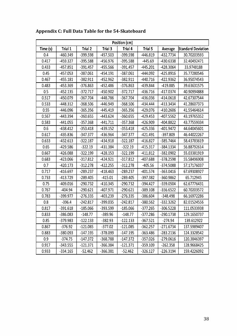
Table 3.0 shows the condensed table displaying the average position and standard deviations for the 54-‐Skateboard. The excluded data is shown in Appendix C. For the 54-‐Skateboard, the time interval that was chosen was between 0.400-‐0.944 seconds for the same reasons as stated in “Determining the Acceleration for the 52-‐Skateboard”. Figure 9.0 below shows a scatter plot showing time on the X-‐axis and the average position of the 54-‐skateboard on the Y-‐axis with an accompanying equation.
The accompanying equation for the graph shown in Figure 9.0 is: 𝑠 𝑡 = 691.52𝑥! − 574.5𝑥 − 306.82
Table 3.0
Figure 9.0

15
Which, with referral to the R2 value of 0.97758, very accurately models the position of the 54-‐Skateboard as a function of time. This equation was obtained using a TI-‐84 calculator and Microsoft Excel. The steps are shown in Determining the Equation from the Raw Data. As stated before in Determining the Acceleration of the 52-‐Skateboard, by taking the second derivative of the function above, the acceleration of the 53-‐Skateboard can be determined. These calculations are shown below: 𝑠(𝑡) = 691.52𝑥! − 574.5𝑥 − 306.82 𝑠! 𝑡 = 𝑣 𝑡 = 1383.04𝑥 − 574.5 s’’(t) = a(t)= 1383.04 Through the calculations shown above, it has been determined that the acceleration of the 53-‐Skateboard was: 1383.04 cms-‐2, which, by metric conversions, is 13.8304 ms-‐2. The Exploration: Mapping the Relationship Between the Diameter of a Wheel and the Skateboard’s Acceleration:
Diameter (mm) Average Acceleration (ms-‐2) 52 10.474 53 12.887 54 13.8304
Table 4.0 above shows the respective calculated accelerations for each skateboard with varying wheel sizes (mm). When graphing the average acceleration as a function of the wheel’s diameter, the expectation was to look at the R2 values and see which trend-‐line could best model the relationship between the acceleration and the wheel size. At a glance, I expected a linear relationship between the acceleration and the wheel diameter. Figure 10.0 shows a graphical representation of the average acceleration as a function of time with a linear trendline.
Table 4.0

16
Figure 10.0 shows a strong linear correlation between the diameter of the wheel (mm) and the average acceleration of the skateboard (ms-‐2) with a linear function of a(D)=1.6782x – 76.547 which has a large R2 value of 0.93993, which suggests that this function is an accurate model . This equation was calculated by plotting the values shown in Table 4.0 into Microsoft Excel in order to create both an equation and obtain the value for R2. Afterwards, the TI-‐84 Calculator was used to reaffirm the authenticity of equation using the method shown in Determining the Equation from the Raw Data. This should have been the end of the exploration however, out of curiosity, I wanted to see if any other trendline could be applied to the data. To my complete surprise, when I plotted the polynomial trendline to the data, I got a function that had an R2 value of 1! This suggested that the quadratic function was a perfect representation of the relationship between the diameter of a wheel and it’s acceleration. This graph is shown below in Figure 11.0.
Logically, the equation with the largest R2 value should be the one that is used to model the relationship between the skateboard and it’s wheel diameter.
Figure 10.0
y"="1.6782x"+"76.547"R²"="0.93993"
10"
10.5"
11"
11.5"
12"
12.5"
13"
13.5"
14"
14.5"
51.5" 52" 52.5" 53" 53.5" 54" 54.5"
Avera
ge'Ac
celera
*on'(
ms02 )'
Diameter'of'Wheel'(mm)'
Diameter'of'Skateboard'Wheel'VS'Average'Accelera*on'(Linear)'
Figure 11.0
y"="$0.7348x2"+"79.567x"$"2140.1"R²"="1"
10"
10.5"
11"
11.5"
12"
12.5"
13"
13.5"
14"
14.5"
51.5" 52" 52.5" 53" 53.5" 54" 54.5"
Avera
ge''A
cceler
a*on
'(ms02)'
Diameter'of'Wheel'(mm)'
Diameter'of'Skateboard'Wheel'VS'Average'Accelera*on'(Polynomial)'

17
Based on this premise, that means that the acceleration of a skateboard can be obtained using this equation a(D) =-‐0.7348D2 + 79.567D – 2140.1 where “a” is the acceleration of the skateboard and D is its diameter. However the fact that this is a quadratic function brings to light several things that don’t necessarily make sense. First, it suggests that there is a maximum value for the diameter of the skateboard which would result in the greatest acceleration. This value, which can be obtained by calculating both the vertex of the quadratic function or by differentiating the function and calculating it’s stationary point, suggests that there is a maximum threshold for the wheel size diameter. By having a threshold, it implies that any diameter greater than the threshold would result in a decrease in acceleration as compared to it’s predecessors and any increase in the diameter converging towards the threshold would result in an increase in acceleration until the threshold has been met. This means that skateboard would slow down if the diameter of the wheel increased passed the threshold. Beyond this, if the relationship is assumed to be modeled by a quadratic function, then there is also the underlying assumption that there are two diameters which would have no acceleration at all. From a mathematical perspective, these diameters would be the X-‐intercepts for the quadratic function. Both the suggestion that there are two diameters which will result in zero acceleration along with one specific diameter that will provide a maximum acceleration and a maximum diameter seems very counterintuitive. This is because first of all, if a skateboard is experiencing zero acceleration, then it means that no matter how hard a rider pushes, he will never be able to speed up. Objects need to accelerate initially in order to start moving. If an object can’t accelerate at all, which is what is implied by this equation, then the object can’t move. Meaning that any skateboard with a diameter at the X-‐intercepts for the equation will not be able to move at all. Beyond this, if there is a threshold for the maximum acceleration and diameter, then it implies that any diameter greater than the threshold will result in the skateboard slowing down. Because of these implications, I have trouble reconciling myself with the quadratic model. It seems very counter intuitive. On the other hand, from Figure 10.0, if we apply this linear relationship to model the relationship between the diameter and the skateboard’s acceleration, it means that by increasing the diameter of the skateboard wheel, the skateboard’s average acceleration will increase as well. This seems like a much more attractive and realistic model as there is no threshold value for the diameter and there is only one value for the diameter which would have zero acceleration as opposed to two values, as proposed in the quadratic model. This linear models seems much more realistic yet by referral to the R2 values, it seems that the quadratic model is the more accurate depiction for the relationship between the diameter of a wheel and it’s acceleration despite all the strange implications that come out of it.

18
The subsequent sections of this investigation will seek to determine the maximum threshold for the quadratic model, the values for the diameter that will have no acceleration, and in the end will try to explain whether this models is an accurate model, despite the large R2 value, and if it is proven that this model was incorrect, will suggest reasons as to why this occurred. The Exploration: Understanding the Quadratic Model: If we are to assume that the equation from the quadratic graph is the true model for the relationship between the wheel size of a skateboard and it’s average acceleration, than by calculating the point of inflexion for the curve we can determine what wheel size would create the maximum acceleration. Our function is: a(D) = −0.7348D! + 79.567D – 2140.1 By taking the first derivative of this function and equating the gradient to 0, we can determine at what value of D will we have a point of inflexion (which should be a maximum but this will be proved later on). This value of D will be the diameter of the wheel that yields the largest possible average acceleration if this model is assumed to be true. So: 𝑎! 𝐷 = −1.4696𝐷 + 79.567 0 = −1.4696𝐷 + 79.567 −1.4696𝐷 = −79.567
𝐷 =−79.567−1.4696
= 54.14194339 =54 Despite getting a decimal an answer, by convention we represent diameters as whole numbers hence why D was simplified to be 54 mm. It is important to note that the unrounded value for D is the real diameter at which there will be maximum acceleration. From the calculations above, we have shown that 54 is a stationary point as it is the value of D when the derivative is equal to zero yet to determine if this is a maximum or a minimum point, the two points 53 and 55 will be used to compare gradients. 53: 𝑎! 53 = ((−)1.4696 53 + 79.567) = 1.6782
ßD is the symbol for diameter (mm)

19
This is a positive value which indicates all values before 54 will have a positive gradient. 55: 𝑎! 55 = ( − 1.4696 55 +79.567)= -‐1.261 As this value is a negative value, this indicates that all values greater than 54 will have a negative gradient. The findings can be summarized in the table below: (D) 53 54 55 a’(D) + 0 -‐ Shape of Curve
Table 5.0 shows the sign for each value of D as well as a depiction of what the curve would look like. This table shows that when D= 54, it is a maximum value. By substituting 54 into the original function, we can determine the maximum possible acceleration for a skateboard wheel. These calculations are shown below: a(D) = −0.7348D! + 79.567D – 2140.1 𝑎 54 = −0.7348 54 ! + 79.567 54 − 2140.1 = 13.8412 The acceleration for a wheel with a diameter of 54 mm is shown to be 13.8 ms-‐2. Based on the calculations above, the maximum possible wheel size that a skateboard can have is 54 mm in diameter and would reach an average acceleration of 13.8 ms-‐2. If the polynomial function is to be applied, then that would indicate that as the wheel size increases passed 54 mm, the average acceleration of the wheel would decrease. This is shown in Figure 12.0 below where the equation for the polynomial is extrapolated to include a domain of 47 mm ≤ x ≤ 62 mm:
Table 5.0

20
The extrapolated accelerations were obtained by inputting 47-‐62 into the value for D for the quadratic function. These findings are summarized below in Table 6.0:
With referral to Figure 12.0, because the graph is a concave-‐down graph where the Y-‐Axis is average acceleration (ms-‐2) and the X-‐axis is the diameter of the wheel (mm), we see that as the value of X increases, the value of Y will decrease as it increases beyond our maximum point of 54 mm. To verify whether 54 is the maximum diameter for a skateboard wheel for there to be the largest possible acceleration, the vertex of the quadratic function will be obtained. These calculations will be shown below:
𝑉𝑒𝑟𝑡𝑒𝑥 = −𝑏2𝑎
y"="$0.7348x2"+"79.567x"$"2140.1"R²"="1"
$36"$33"$30"$27"$24"$21"$18"$15"$12"$9"$6"$3"0"3"6"9"12"15"18"
45" 47" 49" 51" 53" 55" 57" 59" 61" 63"
Average'Ac
celera*o
n'(m
s02)'
Diameter'of'Skateboard'Wheel'(mm)'
Diamater'of'Skateboard'Wheel'VS'Average'Accelera*on'(Extrapolated)'
Figure 12.0
Table 6.0

21
Our function for average acceleration as a function of wheel diameter is in the standard form for a quadratic equation which is:
𝑆𝑡𝑎𝑛𝑑𝑎𝑟𝑑 𝐹𝑜𝑟𝑚 = 𝐴𝑥! + 𝐵𝑥 + 𝑐 So by looking at our function:
a(D) = −0.7348D! + 79.567D – 2140.1 We see that: A=-‐0.7348 B= 79.567 and C= 2140.1 So by using our equation for the vertex, we can verify whether 54 is a maximum point.
𝑉𝑒𝑟𝑡𝑒𝑥 = −𝑏2𝑎
= −79.567
2 ∗ − 0.7348 = 54.14194339
This is the exact same value obtained by equating the first derivative to zero and solving for D prior to rounding to the nearest whole number. For the sake of simplification, we can assume that the X coordinate of our vertex is 54 which is the same value that we determined to be the maximum point. Through using both the first derivative to obtain a stationary point and by calculating the vertex for the parabolic curve we have found that if this equation is to be used, then the maximum acceleration will be obtained when the diameter of the wheel is 54 mm. Any wheel with a larger diameter will experience a decrease in it’s acceleration. The first thing that this makes me think is that any diameters greater than 54 will result in the skateboard slowing down rather than increasing in speed as indicated by the decrease in acceleration. Yet this model seems very counter intuitive. Why would an increase in the size of the wheel decrease it’s average acceleration? In this experiment the brand and manufacturing of the wheel remained constant. The amount of force that was applied to the skateboard remained constant as it was rolled from an inclined plane and the only force acting on it was gravity. Though one can say that the increased diameter of the wheel increased the mass of the wheel as it’s overall size was increasing, this could not have slowed down the wheel so much since we were working in a very small range. TO me, this model does not make much sense. Initially, I would assume that the greater the diameter of the wheel, the more distance the wheel could cover in a given time period given that it has a greater circumference.

22
To demonstrate this point, I have produced a proof and an explanation below to explain my theory. The Exploration: Proof: First of all, we have to assume that each wheel is a perfect circle. So if we have Wheel 1 with a radius of 1 meter and Wheel 2 with a radius of 2 meters then we can calculate the distance the wheel will travel in one revolution by calculating the circumference, which we know, is obtained by using the equation:
𝐶𝑖𝑟𝑐𝑢𝑚𝑓𝑒𝑟𝑛𝑒𝑐𝑒 = 2 ∗ 𝑃𝑖 ∗ 𝑅 Wheel 1: If Radius=1 meter, then the circumference is 2 ∗ 𝑃𝑖 ∗ 1 = 6.3 𝑚𝑒𝑡𝑒𝑟𝑠 (2 𝑠𝑖 𝑓𝑖𝑔𝑠) Wheel 2: If the Radius= 2 meters, then the circumference is 2 ∗ 𝑃𝑖 ∗ 2 = 13 meters (2 sig figs) Since we have calculated the circumference for both Wheel 1 and Wheel 2, we can now determine which wheel is faster. By setting a fixed distance of 40 units, if we calculate quotient of 40 and both the circumference of Wheel 1 and Wheel 2, we can determine how many revolutions does the wheel need to make in order to cover this distance. This calculation is shown below: Wheel 1:
𝑅𝑒𝑣𝑜𝑙𝑢𝑡𝑖𝑜𝑛𝑠 = 406.3 = 6.3 𝑟𝑒𝑣𝑜𝑙𝑢𝑡𝑜𝑖𝑛𝑠 2 𝑠𝑖𝑔 𝑓𝑖𝑔𝑠
Wheel 2:
𝑅𝑒𝑣𝑜𝑙𝑢𝑡𝑖𝑜𝑛𝑠 = 4013 = 3.0 𝑟𝑒𝑣𝑜𝑙𝑢𝑡𝑖𝑜𝑛𝑠 2 𝑠𝑖𝑔 𝑓𝑖𝑔𝑠
If both wheels were pushed down an inclined plane with the same amount of force and frictional forces were considered negligible, then from the calculation shown above, we can conclude that Wheel 2, the wheel with the larger diameter, would cover the same distance as wheel 1 in fewer spins. This means that wheel 2 is moving faster than wheel one because it can cover more distance than wheel 1 in a given time. We can prove this even further by setting a fixed number of revolutions and seeing which wheel would cover more distance. Lets say we want to calculate the distance traveled for both wheels in ten revolutions, from the calculations below, we will see that the wheel with the larger radius will cover more distance in the same amount of revolutions: We can use cross multiplication to determine the total distance travelled by each wheel. This is shown below:

23
Wheel 1:
𝐷𝑖𝑠𝑡𝑎𝑛𝑐𝑒 𝑇𝑟𝑎𝑣𝑒𝑙𝑙𝑒𝑑 =6.3 𝑚𝑒𝑡𝑒𝑟𝑠1 𝑅𝑒𝑣𝑜𝑙𝑢𝑡𝑖𝑜𝑛 =
𝑋 𝑚𝑒𝑡𝑒𝑟𝑠10 𝑅𝑒𝑣𝑜𝑙𝑢𝑡𝑖𝑜𝑛𝑠
𝑋 = 6.3 ∗ 10
= 63 The first function represents the circumference of the wheel. Within just one revolution, the wheel would have travelled the distance of its circumference. By using cross multiplication, we can use this conversion to determine the distance that the wheel would travel if it were to undergo 10 revolutions. For Wheel 2 the exact same procedure will be used as shown below. Wheel 2:
𝐷𝑖𝑠𝑡𝑎𝑛𝑐𝑒 𝑇𝑟𝑎𝑣𝑒𝑙𝑙𝑒𝑑 =13 𝑚𝑒𝑡𝑒𝑟𝑠
1 𝑅𝑒𝑣𝑜𝑙𝑢𝑡𝑖𝑜𝑛 =𝑋 𝑚𝑒𝑡𝑒𝑟𝑠
10 𝑅𝑒𝑣𝑜𝑙𝑢𝑡𝑖𝑜𝑛𝑠
𝑋 = 13 ∗ 10 = 130
From this, we can see that Wheel 2 will cover a greater distance in the same amount of revolutions as Wheel 1. This shows that the greater the diameter of the wheel, the more distance the wheel can travel per revolution which means that the greater the diameter of the wheel, the greater it’s speed. Yet despite this proof, the polynomial function completely contradicts the logic of this proof. The polynomial models suggest that after the threshold diameter, the skateboard’s acceleration would decrease and ultimately slow down. Beyond this, my biggest issue with this quadratic model was that it also assumed that there were two diameters for the wheels, which would result in no acceleration whatsoever. We can see this by using the Quadratic Formula to calculate the X-‐intercepts of our function, which represents the wheel size diameters that have zero acceleration. The Quadratic Formula is:
𝑋 =−𝐵 ± 𝐵! − 4𝐴𝐶
2𝐴

24
So by inputting our quadratic function, which shows the acceleration of the skateboard as a function of its wheel diameter into the quadratic equation, we can calculate both wheel sizes that experience zero acceleration. So our original equation is:
a(D) = −0.7348D! + 79.567D – 2140.1 Where: A= -‐0.7348 B= 79.567 And C= -‐2140.1 By inputting these values into the quadratic function, we can calculate the diameters of the wheel, which apparently will have no acceleration. These calculations are shown below:
𝐷 =−𝐵 ± 𝐵! − 4𝐴𝐶
2𝐴
𝐷 =−79.567± 79.567! − 4(−0.7348)(−2140.1)
2 −0.7348
𝐷 =−79.567± 6330.907489 − (6290.18192)
2 −0.7348
𝐷 =−79.567± 40.725569
−1.4696
𝐷 =−79.567± (6.381658797)
−1.4696 From this function, we can calculate both diameters that will have an acceleration of zero, which will be referred to as D1 and D2, respectively from this point on. .
𝐷! =−79.567+ 6.381658797
−1.4696 = 49.79949728 = 49 (2 𝑠𝑖𝑔. 𝑓𝑖𝑔𝑠)
As shown above, D1 , which is one of the two diameters which would result in zero acceleration, is 49 mm. With the calculation for D1, (-‐)B was added to the square root of B2-‐4AC.

25
The calculation for D2, which is the second diameter in which the acceleration is zero, is shown below:
𝐷! =−79.567− 6.381658797
−1.4696
=−(85.9486588)
−1.4696 = 58.48438949
= 58 2 𝑠𝑖𝑔. 𝑓𝑖𝑔𝑢𝑟𝑒𝑠 As shown above, D2 is equal to 58 mm. it is important to note that in this calculation (-‐)B was subtracted from the square root of B2-‐4AC. Although in Table 6.0 the values for D1 and D2 are shown to have non-‐zero accelerations, the values were simplified with no decimals to represent them in a familiar and conventional form. The true values for D1 and D2 at which the acceleration is zero is the unrounded form shown above. Although the maths makes sense and the R2 value was a perfect match, I don’t like how the polynomial model suggests that when the wheel diameter is 48 mm or 58 mm, the skateboard experiences no acceleration at all. This is incredibly counter intuitive because when the skateboard was released down the incline plane, the only force acting on it was gravity, which means that the skateboard should experience some sort of acceleration as there was a force acting on it. By Newton’s second law, the Acceleration is directly proportional to the force that the object experiences. This is related by the following equation:
𝐹 = 𝑚 ∗ 𝑎 Where F is the force in Newtons, m is the mass of the object in kilograms, and a is the acceleration in ms-‐2. Since mass is always constant, we can see that acceleration is directly proportional to the force. And when gravity acts on an object, it exerts a downward force indicating by Newton’s second law that the object must be accelerating (Newton’s Second Law). Yet this quadratic model contradicts this very well established law of Physics, which makes me seriously question the accuracy of this model despite the large R2 value. Upon serious contemplation about the implications of the quadratic model, I realized that I had a serious misconception about the very nature of acceleration. Initially, I had believed that any value passed the threshold of 54 mm would result in the skateboard slowing down which to me seemed incredibly counter intuitive as this is what I believed a decrease in acceleration implied. But later on, I realized that a particle could still have negative acceleration and still be speeding up!

26
Based off of this premise, I believe that if I can prove that the skateboard is not slowing down after the threshold value, then the implications that I had put forth before about the quadratic model can be negated and we can then assume that the linear model is the more accurate way of representing the data, as this suggests that the greater the diameter, the more the skateboard will speed up. This belief is also supported by the proof shown above. In short, I aim to prove that as the diameter increases, the skateboard never slows down but rather, continues to speed up. Doing this is very simple, we can figure out if an object is speeding up or slowing down if both the acceleration and its velocity have the same sign and are in the same direction. For example, if a particle has a positive velocity (denoted by a “+”) and a positive acceleration, then it is speeding up. If a particle has a negative velocity (denoted by a “-‐“) and a negative acceleration, then it is also speeding up. However, if a particle has a positive velocity and a negative acceleration or vice versa, then it is slowing down. The reason why a particle with both a negative acceleration and velocity is actually speeding up is because of the vector nature of these quantities. If the velocity of a particle is negative, then it is simply moving in the negative direction, and if it’s acceleration is negative, then it’s velocity is simply increasing in the negative direction, which the particle is moving in to begin with. This would result in an overall increase in speed. This is the same premise that is to be applied if the particles had opposite sign accelerations and velocities. If the velocity of a particle was positive, then it is indicating then it is travelling in the positive direction and if it’s acceleration is negative, then it shows that the particle is accelerating in the negative direction, which is in the opposite direction of the particles moment. So essentially, the negative sign indicates deceleration, which is the rate at which the velocity decreases per unit time, which is why the particle would slow down when it’s acceleration and velocity have opposite signs as the particle is travelling in the opposite direction at which the particle is accelerating. Based off of this premise, I believe that I will be able to prove that the polynomial model is actually incorrect and was attributed to several flaws in the experiment, which will be explained below. To do this, I believe that if I take the acceleration of skateboard for different wheel diameters, by integrating the acceleration with respect to time and determine its velocity, I will be able to look at the signs for the acceleration and the integrated velocity and determine if the skateboard is actually slowing down or speeding up. The significance of doing this is because initially, I had believed that the quadratic model suggested that the skateboard was in fact slowing down whenever it had negative acceleration. However, I believe that if I can prove that the skateboard is actually speeding up, then I can disprove the quadratic model. If corret, in the end I

27
will explain what caused the quadratic model to have the larger R2 value compared to the linear model. From Table 6.0, the following values were obtained and will be used to preform this calculation as shown in Table 7.0. Table 7.0 Diameter (mm)
Acceleration (ms-‐2)
47 -‐23.6242
51 6.6022
54 13.8412
55 13.3150
61 -‐20.70398
I have taken great care in choosing the values that I will integrate. The values that I have chosen are accelerations that have a corresponding diameter less than D1 in the negative Y quadrant, less than the threshold value in the positive Y-‐Quadrant, the threshold diameter value (54 mm), a diameter that has an acceleration greater than the threshold value in the Y-‐Quadrant, and an acceleration with a corresponding diameter greater than D2. I believe that if the integrated velocity for each of these accelerations has the same sign as it’s acceleration, then I would have proved that the acceleration of the skateboard wheel is proportional to wheel size. This is because if both velocities and accelerations have the same sign, then it indicates that the particle is speeding up. By choosing values from all quadrants, I hope to show that the particle continues to speed up with increasing wheel size. If this is shown to be the case, then it means that the quadratic model was incorrect, there is no threshold, and there are no two values at which the particle is moving at zero acceleration. So for the following calculations, the domain for the time for each velocity will be from 0-‐5 seconds. This domain was chosen arbitrarily. It does not matter what the time domain for the velocity is so long as it remains constant for each calculation. The purpose of using a definite integral was to eliminate the need to calculate a value for the constant of integration. These calculations will be shown below: The Exploration: Integrating to find the Velocity for the 47-‐Skateboard: When the diameter was 47 mm, its acceleration was extrapolated to be (-‐)23.6242 ms-‐2. The integration of this function to determine the velocity will be shown below:

28
𝑉 𝑇5 − 𝑇0 = 𝑎 𝑡 𝑑𝑡 = −23.6242 𝑑𝑡 = −23.6242 5 − −23.6242 05
0
5
0
= −118.121 The velocity when the diameter of the skateboard’s wheel was 47 mm was integrated to be (-‐)118.121 ms-‐1. The acceleration was also (-‐)23.6242. Since both functions have the same sign, it can be deduced that the particle’s speed is increasing at this point. This is the velocity before D1. The same method seen above will be carried for the remaining accelerations. The Exploration: Integrating to find the Velocity of the 51-‐Skateboard: When the diameter of the wheel was 51mm, it’s acceleration was found to be 6.6022 ms-‐2. The integration of this function to determine the velocity will be shown below:
𝑉 𝑇! − 𝑇! = 𝑎 𝑡 𝑑𝑡 = 6.6022 𝑑𝑡 = 6.6022(5) − 6.6022 0!
!
!
!
= 33.011 The velocity when the diameter of the skateboard’s wheel was 51 mm was integrated to be (+) 33.011ms-‐1. The acceleration was also (+) 6.6022 ms-‐2. Since both functions have the same sign, it can be deduced that the particle’s speed is increasing at this point. This is the velocity after D1 and before the threshold. The Exploration: Integrating to find the Velocity of the 54-‐Skateboard: When the diameter of the wheel was 54 mm, its acceleration was found to be 13.8412 ms-‐2. The integration of this function to determine the velocity will be shown below:
𝑉 𝑇! − 𝑇! = 𝑎 𝑡 𝑑𝑡 = 13.8412 𝑑𝑡 = 13.8412(5) − 6.6022 0!
!
!
!
= 69.206 The velocity when the diameter of the skateboard’s wheel was 54 mm was integrated to be (+) 69.206 ms-‐1. The acceleration was also (+)13.8412 ms-‐2. Since both functions have the same sign, it can be deduced that the particle’s speed is increasing at this point. This is the value for the velocity at the threshold.

29
The Exploration: Integrating to find the Velocity of the 55-‐Skateboard: When the diameter of the wheel was 55 mm, its acceleration was found to be 13.8412 ms-‐2. The integration of this function to determine the velocity will be shown below:
𝑉 𝑇! − 𝑇! = 𝑎 𝑡 𝑑𝑡 = 13.3150 𝑑𝑡 = 13.3150(5) − 13.3150 0!
!
!
!
= 66.575 The velocity when the diameter of the skateboard was 55 mm was integrated to be (+) 66.575 ms-‐1. The acceleration was also (+)13.3150 ms-‐2. Since both functions have the same sign, it can be deduced that the particle’s speed is increasing at this point. This is the velocity after the threshold but before D2. The Exploration: Integrating to find the Velocity of the 61-‐Skateboard: When the diameter of the wheel was 61 mm, its acceleration was found to be -‐20.7038 ms-‐2. The integration of this function to determine the velocity will be shown below:
𝑉 𝑇! − 𝑇! = 𝑎 𝑡 𝑑𝑡 = −20.7038 𝑑𝑡 = −20.7038(5) — 20.7038 0!
!
!
!
= −103.519 The velocity when the diameter of the skateboard was 61 mm was integrated to be (-‐) 103.519 ms-‐1. The acceleration was also (-‐) 20.7038 ms-‐2. Since both functions have the same sign, it can be deduced that the particle’s speed is increasing at this point. This is the velocity after D2. Just to summarize the calculated values:
• When the diameter was 47mm, it’s velocity between 0 and 5 seconds was (-‐)118.121 ms-‐1 and it’s acceleration was (-‐)23.624 ms-‐2. This was the value before D1.
• When the diameter was 51 mm, it’s velocity between 0 and 5 seconds was (+)33.011 ms-‐1 and it’s acceleration was (+)6.6022 ms-‐2. This was the value after D1 and before the threshold.
• When the diameter was 54 mm, it’s velocity between 0 and 5 seconds was (+)69.206 ms-‐1 and it’s acceleration was (+)13.8412 ms-‐2. This was the value at the threshold.
• When the diameter was 55 mm, the skateboard’s velocity was (+)66.575 ms-‐1 and it’s acceleration was (+)13.3150 ms-‐2. This was the value after the threshold but before D2.

30
• Finally, when the diameter was 61 mm, it’s velocity was calculated to be (-‐) 103.519 ms-‐1 and it’s acceleration was (-‐) 20.7038 ms-‐2. This was the value after D2.
Conclusion: Final Results From the calculations made above, it is shown that as the diameter of the wheel increases, the skateboard continues to speed up despite having a negative acceleration. The fact that the skateboard is speeding up for diameters even after the threshold diameter size negates the previous belief that the skateboard was slowing down as previously inferred by the quadratic function that plotted the acceleration of the skateboard as a function of it’s wheel diameter. The belief that the skateboard slows down passed the threshold value was a problem on my behalf regarding the concepts of acceleration. By showing that the skateboard is speeding up as the diameter increases, I believe that this is definite proof for the authenticity of the linear model that was proposed in Figure 10.0 which suggests that as the diameter increases, so will the average acceleration. The main issue that I have with the quadratic model is the suggestion of two wheel diameters at which there will be no acceleration. As we have shown that despite having a negative acceleration, the skateboard is increasing in speed, I believe that this shows that the linear model is an accurate depiction of the relationship between the diameter of the skateboard wheel and its acceleration. With this new model, there is no maximum diameter or threshold value that can be calculated seeing as it is a linear curve.
𝑎 𝐷 = 1.6782𝑥 − 76.54 𝑎 𝐷 ! = 1.6782
From the calculation above, we see that if we take the first derivative of our linear function, we lose the D variable meaning we cannot equate the equation to zero and determine a maximum or minimum point. This shows that there are no maximum or minimum points for this model suggesting that if we increase the diameter of the skateboard, we should get an increase it’s acceleration as well. Based on the calculations above, it can be deduced that although the Polynomial/Quadratic function had given a perfect R2 value of 1, it can be concluded that this is not an accurate model for depicting the relationship between the acceleration of a skateboard and the diameter of it’s wheels. Instead, it can be concluded that the more appropriate model is the linear model which has an equation of a(D)= 1.6782D -‐76.547 with an R2 value of 0.93993. Therefore, based off of this premise, we can conclude that the larger the diameter of a skateboard wheel,

31
the faster the skateboard will go. This claim was backed up by both the experimental results and the proof put forth before. Conclusion: How could this Exploration Have been Improved? One of the biggest pitfalls of this exploration was the fact that the polynomial function for the average acceleration as a function of the diameter of the skateboard wheel had given a perfect R2 value suggesting a perfect correlation. However, as stated before, this would have been problematic as it suggested a supposed maximum acceleration a skateboard could travel at while suggesting certain diameters of the wheel for which the skateboard would not accelerate at all. I believe that the data in itself was flawed and did not have a wide enough range which meant that small anomalies in preforming the experiment would have significant effects on the results. The fact that only a small range of diameters was used really hindered the accuracy of this experiment. In this experiment only three different diameters were used (52, 53, and 54 mm) that were all within close proximity of one another. This meant that there was both limited data available to really test how the diameter wheel size affected acceleration while at the same time, made it necessary to extrapolate data and create potential possible accelerations for varying diameters, all from limited data. Since only a small range of data was used, it is very possible that the trend proposed in the conclusion could only apply to skateboard wheels between 52-‐54 mm. Had other wheel diameters been used in the 40’s or even in the 60’s, we would have had sufficient data to create an accurate model for the relationship between the wheel’s diameter and the skateboard’s acceleration. In real life, we see skateboard wheels with diameters greater than 70 mm or even 90 mm. The fact that this experiment was constrained only to diameters in the 50s severely limits the accuracy of the model that we have proposed above One of my biggest issues with this experiment and the linear model is the fact that it suggests that the acceleration would increase infinitely as the diameter increases however, realistically, we don’t see skateboard wheels that are 1 meter in diameter or even greater. There is definitely a limit as to what size a wheel can be in order to experience maximum acceleration. Ultimately, being constrained to a small range and having limited data meant that any errors or mistakes made while carrying out the experiment would significantly affect the final result.

32
If we had a greater range of wheel diameters, I believe that at one point, we would reach a limit in which there is a maximum acceleration that no increase in the diameter will result in an increase in acceleration. I believe that there definitely has to be some limit for the diameter of the wheel to ensure maximum speed. I think theoretically speaking, the greater the size of the wheel, the faster it will go however when it comes to practicalities, skateboards are not very big so using massive wheels that are a foot large or so would not be a viable way to increase the speed of the skateboard as it simply just would not fit on conventional skateboards. Beyond this, I believe that there were significant errors in the data collection of this experiment which could have resulted in the polynomial function having the large R2 value. This can be shown by looking at the average of the standard deviations for each skateboard. Reproduced below is the condensed form of Table 1.0, which shows the position of the skateboard as a function of time for each trial for the 52-‐Skateboard:
For the calculation showing how the standard deviation was obtained, positions of the 52-‐Skateboard when the time was 0.267 seconds will be used. The equation for Standard Deviation is:
𝑆𝑡𝑎𝑛𝑑𝑎𝑟𝑑 𝐷𝑒𝑣𝑖𝑎𝑡𝑖𝑜𝑛 =(𝑥 − 𝑥)!
𝑛 − 1
Where: 𝑋 = 𝑀𝑒𝑎𝑛 𝑃𝑜𝑠𝑖𝑡𝑖𝑜𝑛𝑠
𝑁 = 𝑁𝑢𝑚𝑏𝑒𝑟 𝑜𝑓 𝑋 𝑣𝑎𝑙𝑢𝑒𝑠 𝑋 = 𝑃𝑜𝑠𝑖𝑡𝑖𝑜𝑛 𝑜𝑓 𝐵𝑎𝑙𝑙𝑜𝑜𝑛 𝑎𝑡 𝑡𝑖𝑚𝑒 (𝑡)
To determine the mean (𝑋), the following equation should be used:
𝑀𝑒𝑎𝑛 =(𝑋! + 𝑋! + 𝑋!… )
𝑛 Where X1 and preceding values represent a specific value in the data set. In this case, the subscript denotes the trial number and the value of X is the corresponding value
Time%(s) Trial%1 Trial%2 Trial%3 Trial%4 Trial%5 Average Standard%Deviaton0.267 &430.801 &424.601 &429.985 &448.157 &457.771 &438.263 14.04730.283 &429.399 &423.444 &428.583 &447.075 &456.954 &437.091 14.24790.300 &427.035 &421.305 &426.928 &445.404 &457.011 &435.5366 15.06190.317 &425.339 &418.846 &424.87 &444.266 &455.918 &433.8478 15.60200.333 &422.994 &416.735 &422.296 &443.069 &455.595 &432.1378 16.48820.350 &421.038 &413.953 &419.912 &441.564 &454.948 &430.283 17.28670.367 &419.052 &411.067 &417.301 &439.25 &454.022 &428.1384 17.92260.383 &416.24 &408.131 &414.714 &437.158 &453.029 &425.8544 18.68750.400 &413.954 &404.575 &411.645 &434.932 &453.187 &423.6586 20.0107
Position%(cm)Table 1.0

33
for the position at the designated time and N denotes the number of values in the data set. The calculation for the mean is shown below:
𝑀𝑒𝑎𝑛 =( − 430.801 + − 424.601 + − 429.985 + − 448.157 + − 457.771)
5
=-‐438.263 After calculating the mean, the standard deviation for the position of the skateboard at 0.267 seconds can be obtained. This calculation is shown below. 𝑆𝑡𝑎𝑛𝑑𝑎𝑟𝑑 𝐷𝑒𝑣𝑖𝑎𝑡𝑖𝑜𝑛
=(430.801 − (−)438.263)2 + (424.601 − (−)438.263)2 + (429.985 − (−)438.263)2 + (448.157 − (−)438.263)2 + (457.771 − (— )438.263)2
5 − 1
= 14.0473 This same calculation was preformed for each position value as a function of time for all the values for the 52-‐Skateboard, 53-‐Skateobard, and 54-‐Skateboard to obtain the standard deviation. Each respective Standard Deviation can be seen in Tables 1.0, 2.0, and 3.0 and in the appendix. To determine if there was an error or mistake in preforming the experiment, by taking the average of all the standard deviations for each respective skateboard, we can see which skateboard’s data had the largest range of values which would indicate a mistake in the procedure of the experiment. The Average Standard Deviations for each Skateboard diameter are shown below: Table 8.0
Diameter (mm) 52 53 54 Average Standard Deviation 36.90879975 35.06270332 69.47102138 Each standard deviation was calculated in the same way that was shown above and the average was calculated by taking the sum of all the standard deviations for each wheel diameter and dividing it by the number of values in the series. These values for the standard deviations were obtained from the complete raw data tables for the 52-‐Skateboard, 53-‐Skateboard, and 54-‐Skateboard which is shown in Appendix A, B, and C, respectively. Based off of the results from Table 8.0, it is seen that the 54-‐Skateboard had the largest range of values as noted by having the largest average standard deviation. It is clear that there must have been some anomaly in the experiment because by taking a look at Table 8.0, in both the 52-‐Skateboard and 53-‐Skateboard the average standard deviation was well within the same range of one another. The large jump in

34
average standard deviation values shown in the 54-‐Skateboard shows that there must have been some problems in the actual experiment. This could have been attributed to only taking the X-‐Component of the displacement. It is possible that as the skateboard was making it’s descent, because it was moving so fast, it went out of control and slowed down. As stated in the proof, the greater the diameter of the wheel, the more distance it should cover in a fixed amount of time therefore it should have a greater velocity. This could be why the quadratic model better fit the data. If we were to go by the assumption that the greater the diameter, the faster the skateboard, then it seems plausible that the large velocity of the skateboard could have resulted in the skateboard drastically losing control if it were to hit a crack in the ground or even a pebble. This would ultimately affect the value of the X-‐Component drastically as the skateboard’s path of descent changed and started to move in the Y-‐direction. This could be why the average acceleration for the 54-‐Skateboard was less than the average acceleration for the 53-‐Skateboard which is why, when the Acceleration was plotted as a function of diameter, the quadratic trendline was better able to model the data-‐ because the 54-‐skateboard had spun out of control into the Y-‐Direction. This meant that the skateboard would take longer to complete the descent down the inclined plane which is why the acceleration for the 54-‐Skateboard was calculated to be lower than that of the 53-‐Skateboard. The Conclusion: Final Concluding Remarks: Despite several key faults in the actual experiment and some doubt regarding the legitimacy of the final results and equation, I believe the information garnered through this investigation can be of utmost importance. By understanding how the diameter of a skateboard wheel influences the skateboard’s acceleration, as stated before, riders of all levels can make better buying choices on how to maximize the benefit from their product, parents can ensure that their kids are riding as safely and as slowly as possible, and skateboard manufacturers can use this information in creating newer wheels that are either faster with larger diameters, or safer and slower with smaller diameters. Beyond the realm of skateboarding, the principle of increasing the diameter of a wheel to increase acceleration can be applied to the automobile industry as well. Sports car manufactures such as Ferrari can use this information to create wheels that could allow their cars to go faster. For anything that involves using wheels for motion, speed and safety is often the first consideration. So whether it’s for sports or for transport, the information obtained through this experiment can be an incredible asset. Word Count: 10,117

35
Works Cited
Cox, Elena. "What Is Friction? - Definition, Formula & Forces." Education Portal. N.p.,
n.d. Web. 22 Nov. 2014. <http://education-portal.com/academy/lesson/what-is-
friction-definition-formula-forces.html#lesson>.
"Guide for Texas Instruments TI-83, TI-83 Plus, or TI-84 Plus Graphing Calculator."
Houghton Mifflin Company, n.d. Web. 21 Nov. 2014.
<http://college.cengage.com/mathematics/latorre/calculus_concepts/4e/assets/st
udents/gcp/latorre_4e_grcalcguide.pdf>.
"Newton's Second Law." The Physics Classroom. The Physics Classroom, n.d. Web. 21
Nov. 2014. <http://www.physicsclassroom.com/class/newtlaws/Lesson-
3/Newton-s-Second-Law>.
Appendices

36
Appendix A: Full Data Table for the 52-‐Skateboard:

37
Appendix B: Full Data Table for the 53-‐Skateboard:
38
Appendix C: Full Data Table for the 54-‐Skateboard