THE AERODYNAMIC ANALYSIS OF BWB BASELINE II

E5-8 UAV WITH CANARD ASPECT RATIO (AR) OF 8 AT

ANGLE OF ATTACK OF 10 DEGREE AT 0.1 MACH

NUMBER THROUGH CFD SIMULATION AT DIFFERENT

CANARD SETTING ANGLES

MUHAMMAD NAZREEN BIN ZULKARNAIN

(2008400848)

BACHELOR ENGINEERING (HONS) (MECHANICAL)

UNIVERSITI TEKNOLOGI MARA (UiTM)

JULY 2012

“I/We declared that this thesis is the result of my/our own work except the ideas and

summaries which I/We have clarified their sources. The thesis has not been accepted for

any degree and is not concurrently submitted in candidature of any degree.”

Signed : ………………………..

Date : …………………....

Muhammad Nazreen Bin Zulkarnain

UiTM No : 2008400848

“I declared that I read this thesis and in our point of view this thesis is qualified in term

of scope and quality for the purpose of awarding the Degree of Mechanical Engineering

(Hons) Mechanical.”

Signed : ……………………..

Date : ……………………..

Supervisor or Project Advisor

Prof. Dr. Wirachman Wisnoe

Faculty of Mechanical Engineering

MARA University of Technology (UiTM)

40450 Shah Alam

Selangor

Signed : ……………………..

Date : ……………………..

Co- Supervisor

Puan Zurriati Mohd. Ali

Faculty of Mechanical Engineering

MARA University of Technology (UiTM)

40450 Shah Alam

Selangor

Accepted :

Signed : ……………………….

Date : ……………………….

Course Coordinator

Wan Sulaiman Bin Wan Mohamad

Faculty of Mechanical Engineering

MARA University of Technology (UiTM)

40450 Shah Alam

Selangor

i

Page Title

THE AERODYNAMIC ANALYSIS OF BWB BASELINE II E5-8 UAV WITH

CANARD ASPECT RATIO (AR) OF 8 AT ANGLE OF ATTACK OF 10

DEGREE AT 0.1 MACH NUMBER THROUGH CFD SIMULATION AT

DIFFERENT CANARD SETTING ANGLES

MUHAMMAD NAZREEN BIN ZULKARNAIN

(2008400848)

A thesis submitted in partial fulfillment of the requirements for the award of Bachelor

Engineering (Hons) (Mechanical)

Faculty of Mechanical Engineering

Universiti Teknologi MARA (UiTM)

JULY 2012

ii

ACKNOWLEDGEMENT

In the name of Allah the Most Gracious, Most Merciful, I would like to express

my greatest gratitude for giving me the strength and patience to overcome the challenges

and difficulties in completing this thesis and also for His Blessings. I would also like to

express my sincere gratitude and appreciation to my supervisor and co-supervisor for

their continuous support, generous guidance, patience and encouragement in the

duration of the thesis preparation until its completion.

I would also like to express my special thanks of gratitude to my project’s

supervisor Prof Dr Wirachman Wisnoe as well as to my co-supervisor Puan Zurriati

Mohd Ali who gave me the golden opportunity to do this great project and also for their

continuous support, generous guidance, patience and encouragement in the duration of

the thesis preparation until its completion.

Last but not least, I also like to express my sincere gratitude and appreciation to

my friends who helped me a lot when I am in difficulties in finishing this project. A

million thanks to all who involved in this project. Thank you very much and may Allah

bless all of you and repay your kindness.

iii

ABSTRACT

This thesis represented the study on aerodynamic of a Blended Wing Body

(BWB) with canard aspect ratio of 8 for various canard angle of deflection at angle of

attack 10° by using Computational Fluid Dynamics (CFD) software. The objectives of

this project are to obtain the aerodynamics characteristic such as lift (CL), drag (CD), and

pitching moment coefficient (CM); to analyze the result obtained through CFD

simulation and to acquire the CFD visualization of pressure and Mach contour. The

CAD design of BWB is obtained from the previous research and the design is modified

with a rectangular canard placed in front of the main wing. The CAD format file is

converted to parasolid format for it to be readable by NUMECA software. Generally,

there are three stages of processes in NUMECA: pre-processing, processing and post-

processing. In NUMECA, Fine Hexpress is used as the mesher to acquire the appropriate

mesh quality. Then, it use a solver for the CFD simulation process known as Fine Hexa

by using Spalart-Allmaras turbulence model. The results are analyse by using CFView

in order to obtain the pressure and Mach contour.

iv

TABLE OF CONTENT

Contents

Page Title i

ACKNOWLEDGEMENT ii

ABSTRACT iii

TABLE OF CONTENT iv

LIST OF TABLES vii

LIST OF FIGURES ix

LIST OF ABBREVIATIONS xii

1. INTRODUCTION 1

1.1 Project Title 1

1.2 Project Background 2

1.3 Problem Statement 4

1.4 Objectives of Project 4

1.5 Significance of Project 4

1.6 Scope of Work 5

v

1.7 Methodology 6

2. LITERATURE REVIEW 9

2.1 AERODYNAMICS ANALYSIS 9

2.2 CANARD 12

2.3 BLENDED WING BODY 12

2.4 ASPECT RATIO 14

2.5 MACH NUMBER 15

3. PARAMETER VALIDATION 16

3.1 Selection of Object 18

3.2 Computer Aided Design (CAD) Drawing 18

3.3 Computational Fluid Dynamics (CFD) Simulation 19

3.4 Summary 30

4. GRID SENSITIVITY STUDY 36

4.1 BWB Baseline-II E5 CAD Drawing 38

4.2 CFD Analysis with Variation of Grid Sensitivity 38

4.2.1 Initial Parameters 38

4.2.2 Grid Sensitivity Analysis 41

4.3 Final Parameter Settings 52

4.3.1 Box 52

4.3.2 Faceting 52

4.3.3 Initial Mesh 53

4.3.4 Number of Refinement 53

5. RESULT AND DISCUSSION 54

5.1 Aerodynamic Analysis for BWB Baseline-II E5-8 55

5.1.1 Result of BWB Baseline-II E5-8 CFD Simulation 55

vi

5.1.2 Coefficient of Lift, CL 56

5.1.3 Coefficient of Drag, CD 62

5.1.4 Coefficient of Pitching Moment, CM 64

5.1.5 Pressure Distribution 65

6.0 CONCLUSION AND RECOMMENDATION 67

6.1 Conclusion 68

6.2 Recommendation 68

7.0 REFERENCES 69

APPENDICES 72

APPENDIX A – CAD Drawing of BWB Baseline II E5-8 72

APPENDIX B – Velocity Vectors Flow Visualization 73

APPENDIX B1 – Velocity Vectors Flow Visualization 75

vii

LIST OF TABLES

TABLE TITLE PAGE

Table 3.1 Test condition for surrounding 26

Table 3.2 Test condition for BWB Baseline-II E2 27

Table 3.3 Wind tunnel and Numeca Data 30

Table 4.1 Box parameter 39

Table 4.2 Faceting parameter 39

Table 4.3 Initial mesh parameter 40

Table 4.4 Surrounding Condition 40

Table 4.5 BWB Baseline-II E5 Condition 40

Table 4.6 Variation of box 41

Table 4.7 Minimum length parameter 43

Table 4.8 Curve and Surface Tolerance parameter 45

Table 4.9 Curve Resolution parameter 46

Table 4.10 Surface Resolution parameter 48

Table 4.11 Initial Mesh parameter 49

Table 4.12 Types of Initial Mesh 49

Table 4.13 Number of Refinement parameter 50

Table 4.14 Box parameter 52

viii

Table 4.15 Faceting parameter 52

Table 4.16 Initial Mesh parameter 53

Table 4.17 Number of Refinement parameter 53

Table 5.1 Table of results for BWB Baseline-II E5-8 55

ix

LIST OF FIGURES

FIGURE TITLE PAGE

Figure 1.1 Motion of Aircraft about its Axes [6] 3

Figure 1.2 BWB-Baseline II E5 [5] 3

Figure 2.1 Aircraft Motion [17] 10

Figure 2.2 Forces in Aircraft [18] 11

Figure 2.3 BWB Baseline-I 13

Figure 2.4 BWB Baseline-II 13

Figure 2.5 BWB Baseline-II E2 without canard 13

Figure 2.6 Evolution of BWB in UiTM 14

Figure 3.1 BWB Baseline-II E2 [16] 18

Figure 3.2 Box size parameters 19

Figure 3.3 Position of BWB in the box. 19

Figure 3.4 Box with a hole of BWB Baseline-II E2 after subtracted 20

Figure 3.5 Domain Setting 20

Figure 3.6 BWB Baseline-II E2 with domain 20

Figure 3.7 Boundary Conditions Set up 21

Figure 3.8 Boundary conditions setting 21

Figure 3.9 Initial Mesh setting 22

x

Figure 3.10 Global Paramaters under Mesh Adaptation 22

Figure 3.11 Surface Adaptation for local refinement number 23

Figure 3.12 Viscous layers setting 23

Figure 3.13 Finished mesh of BWB 24

Figure 3.14 Total number of cells 24

Figure 3.15 General properties setting 25

Figure 3.16: Fluid model setting. 25

Figure 3.17: Flow model parameters 26

Figure 3.18 Boundary conditions setting (solid) 27

Figure 3.19 Boundary conditions setting (external) 27

Figure 3.20 Initial solution setting. 28

Figure 3.21 Outputs setting. 29

Figure 3.22 Lift Coefficient, CL vs Angle of Attack, α 33

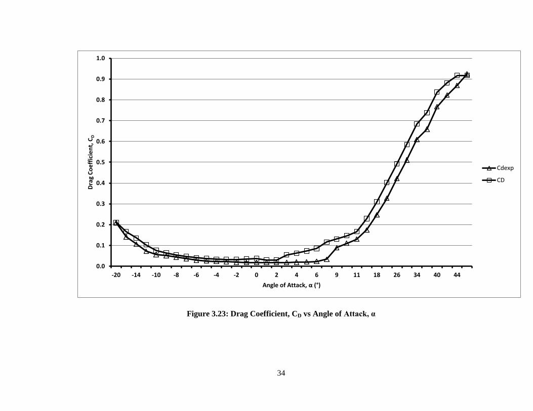
Figure 3.23: Drag Coefficient, CD vs Angle of Attack, α 34

Figure 4.1 L/D Ratio vs No of Cells (Box) 42

Figure 4.2 L/D Ratio vs Number of Cells (Min Length) 44

Figure 4.3 L/D Ratio vs Tolerance 45

Figure 4.4 L/D Ratio vs No of Cells (Curve Resolution) 47

Figure 4.5 L/D Ratio vs No of Cells (Surface Resolution) 48

Figure 4.6 L/D Ratio vs No of Cells (Initial Mesh) 50

Figure 4.7 L/D Ratio vs No of Cells (No of Refinement) 51

Figure 5.1 Lift Coefficient, CL versus Canard Setting Angle, δ 56

Figure 5.2 Mach number at δ = -11°, upper surface 57

Figure 5.3 Mach number at δ = -11°, bottom surface 57

Figure 5.4 Canard’s velocity vector at δ = -11° 58

Figure 5.5 Mach number contour at δ = -3°, upper surface 59

Figure 5.6 Mach number contour at δ = -3°,bottom surface 59

Figure 5.7 Canard’s velocity vectors at δ = -3° 60

Figure 5.8 Mach number contour at δ = 3°, upper surface 61

Figure 5.9 Mach number contour at δ = 3°, bottom surface 61

Figure 5.10 Canard’s velocity vectors at δ = 3° 62

xi

Figure 5.11 Drag Coefficient, CD versus Canard Setting Angle, δ 63

Figure 5.12 Pitching Moment Coefficient, CM versus Canard Setting Angle, δ 64

Figure 5.13 Pressure contours at δ = -11° for upper (left) and lower (right) surfaces 65

Figure 5.14 Pressure contours at δ = -5° for upper (left) and lower (right) surfaces 65

Figure 5.15 Pressure contours at δ = -3° for upper (left) and lower (right) surfaces 65

Figure 5.16 Pressure contours at δ = 3° for upper (left) and lower (right) surfaces 66

xii

LIST OF ABBREVIATIONS

Re Reynold Number

AR Aspect ratio

Ma Mach number

V speed of flow

ρ density

c chord

s span

F force

CL lift coefficient

CD drag coefficient

CM pitching moment coefficient

δ canard setting angle, degree

α angle of attack, degree

1

CHAPTER I

1. INTRODUCTION

1.1 Project Title

The Aerodynamic Analysis of BWB Baseline II E5-8 UAV with Canard Aspect

Ratio (AR) of 8 at Angle of Attack of 10 degree at 0.1 Mach Number through CFD

Simulation at Different Canard Setting Angles.

2

1.2 Project Background

In aircraft, there are two motions that are involve which are translational and

rotational motion. The translational motion is the relative linear position from the origin.

Rotational motion relates to the orientation of the body which consists of yawing,

pitching and rolling [1]. These motions are influenced by the control surfaces; ailerons

(rolling), elevator (pitching) and rudder (yawing) [2]. The pitching motion or

longitudinal motion is influenced by the elevator or canard [3]. Canard is a longitudinal

stabilizer located ahead of the main wing, on the fuselage. There are three types of

canard; lifting canard, control canard and couple canard. However, this project will

focus on control canard. Control canard provides the same function as the aft horizontal

stabilizer by introducing a moment that changes the angle of attack of fuselage and main

wing [4].

From the previous aerodynamics analysis data obtained, the BWB-Baseline II

shows a better result rather than Baseline-I, therefore UITM has continued their study on

Baseline-II until now which is BWB Baseline-II E5 [5]. The BWB-Baseline II E5-8 will

use a rectangular canard as a secondary wing and the primary wing tip will be twisted a

little. The aerodynamics analysis data in this project will be obtained using CFD.

3

Figure 1.2 BWB-Baseline II E5 [5]

Canard

Twisted wing

Figure 1.1 Motion of Aircraft about its Axes [6]

4

1.3 Problem Statement

There are a few setbacks in this project since the data is not available for the

aerodynamic analysis (lift coefficient CL, drag coefficient CD, and pitching moment

coefficient CM) of the BWB Baseline II E5-8. Furthermore, this project is a new research

to study the effect of a rectangular canard on the BWB Baseline II E5.

1.4 Objectives of Project

This project consists of several objectives which are:

1. To obtain lift, drag and pitching moment coefficient.

2. To analyze the result obtained through the CFD simulation.

3. To obtain CFD visualization: pressure and Mach countour, velocity vectors.

1.5 Significance of Project

The significance of this project is obtaining the aerodynamics data for BWB-

Baseline II E5-8 for analyzing the aerodynamic characteristics. Furthermore, the result

from this project can also be included in the database for BWB-Baseline II E5-8.

5

1.6 Scope of Work

This project consists of several scopes of work which are:

1. Model to be used: BWB-Baseline II E5-8

2. Type of Canard to be used: Rectangular Canard with Aspect Ratio (AR) 8

[Area = 0.36 m2]

3. Canard setting angle : -22° to 8°

4. Mach Number 0.1

5. CFD simulation

6. Turbulence models to be use : Spalart-Allmaras turbulence model

6

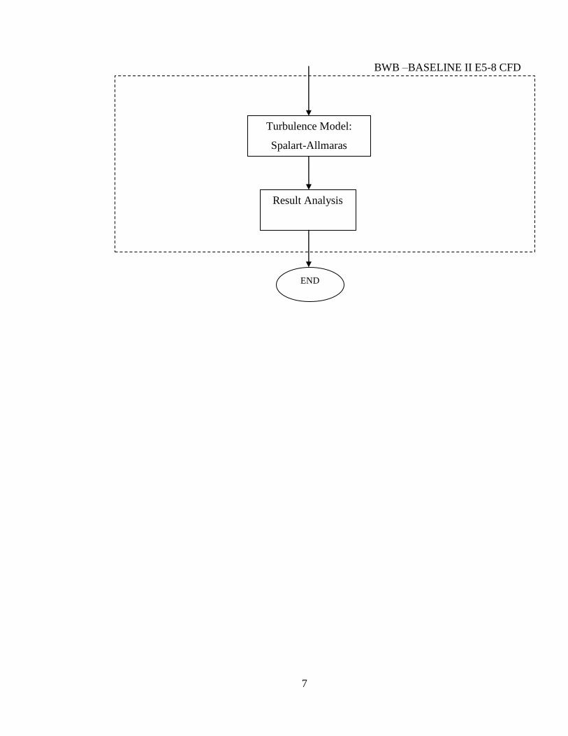
1.7 Methodology

GRID SENSITIVITY STUDY

PARAMETER VALIDATION

START

Literature review

YES

Obtain BWB-Baseline II E5-8

CAD Drawing

CFD Analysis with variation

of grid sensitivity, N

Independence

achieved?

NO

YES

Model Selection

CAD Drawing

CFD Simulation

Data

Validate

?

Reference from

journals/article

NO

7

BWB –BASELINE II E5-8 CFD

ANALYSIS

Turbulence Model:

Spalart-Allmaras

Result Analysis

END

8

Literature Review

To gain basic knowledge on aerodynamic analysis, canard, Blended Wing Body

(BWB) and previous research on books and journals that may help to develop the

project. Literature review will be done throughout the project.

Parameter Validation

Search for any suitable flying model such as wing blade or aerofoil. Then, draw

the model in CAD drawing and do CFD simulation. Next, is to validate the data obtained

from the simulation with the data from the reference journals and books. If the obtained

data is inaccurate with the data from the references, repeat the CFD simulation.

Grid Independence Study

The CAD drawing for BWB-Baseline II E5-8 and rectangular canard with aspect

ratio of 8 are obtained. The model for BWB-Baseline II E5-8 is the half model of the

structure which is to reduce the simulation time by reducing the computer’s memory and

saving time in modeling. Next, the CAD drawing is transferred to CFD to generate

meshing. The analysis will be done by using different meshing sizes to test the L/D ratio.

This process will continue until the L/D ratio approach to constant at certain

no of grid, N.

BWB –Baseline II E5-8 CFD Analysis

Then, the process is continued for the aerodynamic analysis section. Spalart-

Allmaras will be use as the turbulence model at the angle of attack 10° with different

canard setting angles from δ = -22° to δ = 8°. The result will be obtained through the

CFD simulation and graph will be plot where the CL, CD, and CM versus the different

canard setting angle at angle of attack 10°. Then, by using the CFView, we can get the

pressure and Mach contour and also velocity vectors. The data from the CFD simulation

will be analyze and the result will be discussed together with the velocity vectors,

pressure and Mach contour.

9

CHAPTER II

2. LITERATURE REVIEW

2.1 AERODYNAMICS ANALYSIS

2.1.1 Aircraft motion

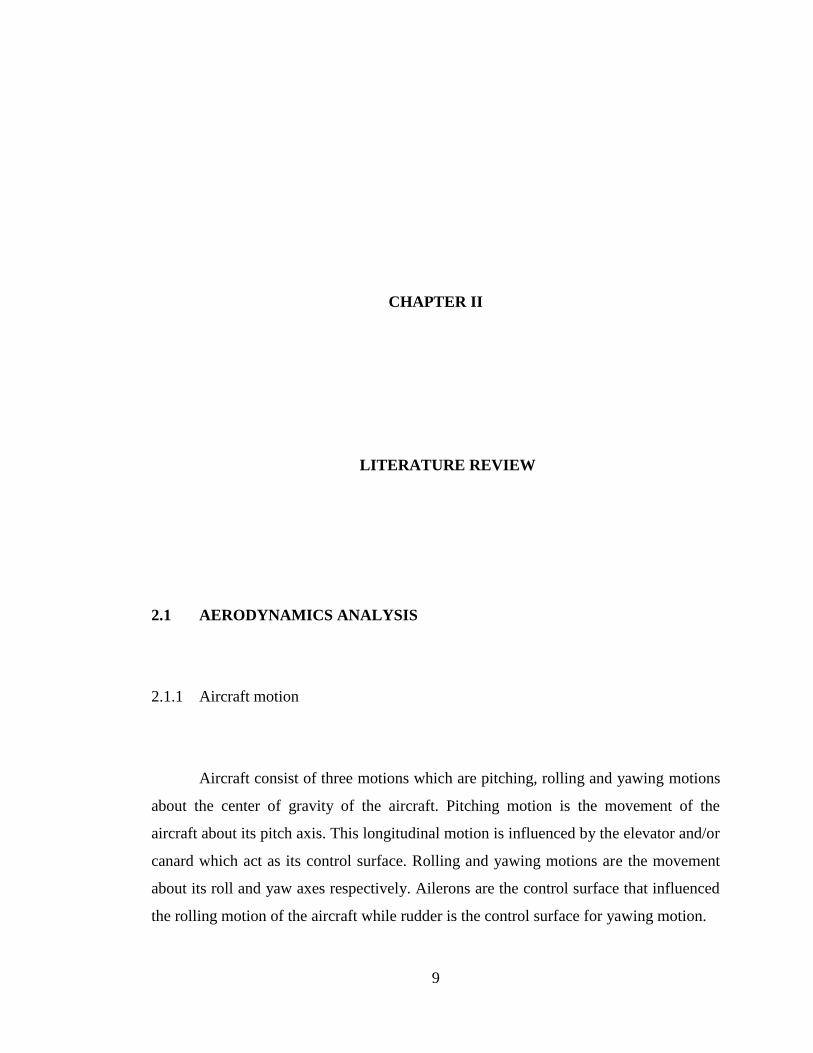
Aircraft consist of three motions which are pitching, rolling and yawing motions

about the center of gravity of the aircraft. Pitching motion is the movement of the

aircraft about its pitch axis. This longitudinal motion is influenced by the elevator and/or

canard which act as its control surface. Rolling and yawing motions are the movement

about its roll and yaw axes respectively. Ailerons are the control surface that influenced

the rolling motion of the aircraft while rudder is the control surface for yawing motion.

10

Figure 2.1 Aircraft Motion [17]

11

2.1.2 Aircraft Forces

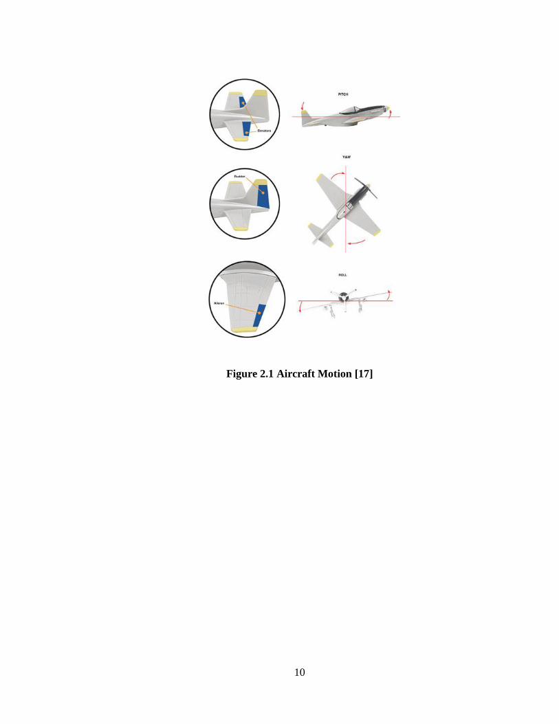
Mainly, there are four forces acted on an aircraft. These forces that are exerted

on the aircraft are lift, thrust, drag and weight forces.

Lift force is the sum of components of the pressure and wall shear forces in the

direction normal to the flow tend to move the body in that direction [7].

Drag on the other hand, is the force that acts in a direction that is opposite to the

motion of the aircraft. Drag is a vector quantity which has magnitude and direction [7].

Figure 2.2 Forces in Aircraft [18]

12

2.2 CANARD

Canard is a longitudinal stabilizer which is located ahead of the primary wing

and on the fuselage [8]. For high performance aircraft, canard-wing configuration is

often required for this type of aircraft design which it need to provide high lift for wide

range of angles of attack in order for it to be maneuverable [9]. There are three types of

canard which are control canard, lifting canard and couple canard. Control canard will

be use in this project which act as the secondary wing and it provide the same function

as the front horizontal stabilizer by introducing a moment that changes the angle of

attack of the fuselage as well as the main wing [10].

2.3 BLENDED WING BODY

Blended Wing Body (BWB) is a concept which was introduced by

Liebeck et. al [11]. Blended Wing Body is a concept where the fuselage and wing is

combined together to form a single body [12]. BWB is a hybrid of flying-wing aircraft

and the conventional aircraft where the body is designed to have a shape of an airfoil

and carefully streamlined with the wing to have a desired planform [13].

2.2.1 History of BWB in UiTM

In University of Technology MARA (UiTM), the research on Blended Wing

Body has been started since 2005. The UiTM’s BWB has been classified as a mini UAV

(Unmanned Aerial Vehicle). There are many types of BWB which are developed by

UiTM for research purposes which are BWB Baseline-I and BWB Baseline-II. BWB

Baseline-I is designed with an elevator for pitching motion. BWB Baseline-II

13

completely revised version from BWB Baseline-I. It has a simpler planform, broader

chord wing and slimmer body compared to BWB Baseline-I. BWB Baseline-II E2

without canard has a slight modification where part of the wing is twisted down at

certain angle [5][14].

Figure 2.3 BWB Baseline-I

Figure 2.4 BWB Baseline-II

Figure 2.5 BWB Baseline-II E2 without canard

14

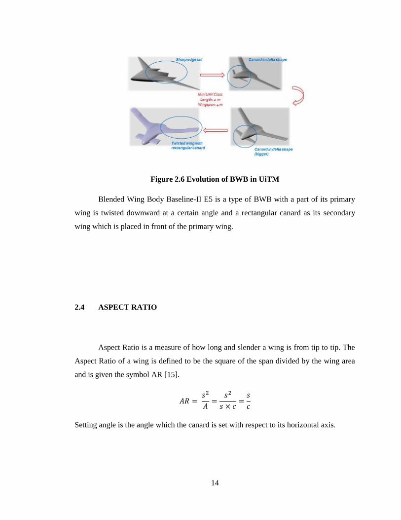
Figure 2.6 Evolution of BWB in UiTM

Blended Wing Body Baseline-II E5 is a type of BWB with a part of its primary

wing is twisted downward at a certain angle and a rectangular canard as its secondary

wing which is placed in front of the primary wing.

2.4 ASPECT RATIO

Aspect Ratio is a measure of how long and slender a wing is from tip to tip. The

Aspect Ratio of a wing is defined to be the square of the span divided by the wing area

and is given the symbol AR [15].

Setting angle is the angle which the canard is set with respect to its horizontal axis.

15

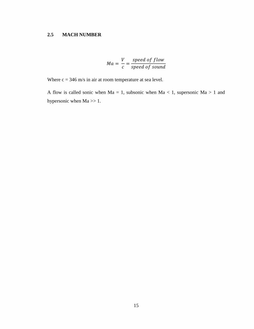
2.5 MACH NUMBER

Where c = 346 m/s in air at room temperature at sea level.

A flow is called sonic when Ma = 1, subsonic when Ma < 1, supersonic Ma > 1 and

hypersonic when Ma >> 1.

16

CHAPTER III

3. PARAMETER VALIDATION

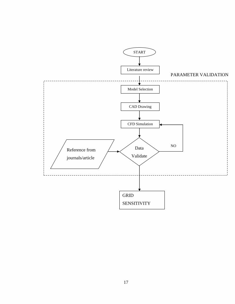
In this chapter, Parameter Validation will be discussed briefly. Parameter

Validation is a process of running a simulation on a selected object with the valid data as

reference from journals. The data that are obtained from the simulation will be compared

to the data in the journal. The main idea of this stage is to obtain the values of lift

coefficient (CL), drag coefficient (CD) and pitching moment (CM) (any which that are

provided in the journal) that is as near as possible to the data from the referred journal.

17

GRID

SENSITIVITY

PARAMETER VALIDATION

START

Literature review

Model Selection

CAD Drawing

CFD Simulation

Data

Validate

?

Reference from

journals/article

NO

18

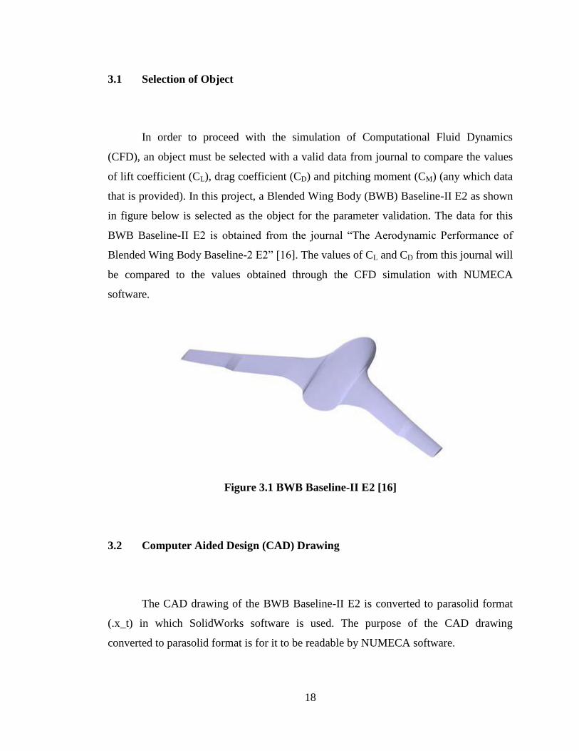
3.1 Selection of Object

In order to proceed with the simulation of Computational Fluid Dynamics

(CFD), an object must be selected with a valid data from journal to compare the values

of lift coefficient (CL), drag coefficient (CD) and pitching moment (CM) (any which data

that is provided). In this project, a Blended Wing Body (BWB) Baseline-II E2 as shown

in figure below is selected as the object for the parameter validation. The data for this

BWB Baseline-II E2 is obtained from the journal “The Aerodynamic Performance of

Blended Wing Body Baseline-2 E2” [16]. The values of CL and CD from this journal will

be compared to the values obtained through the CFD simulation with NUMECA

software.

Figure 3.1 BWB Baseline-II E2 [16]

3.2 Computer Aided Design (CAD) Drawing

The CAD drawing of the BWB Baseline-II E2 is converted to parasolid format

(.x_t) in which SolidWorks software is used. The purpose of the CAD drawing

converted to parasolid format is for it to be readable by NUMECA software.

19

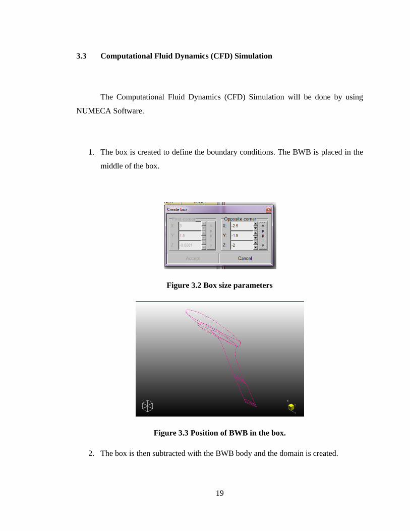
3.3 Computational Fluid Dynamics (CFD) Simulation

The Computational Fluid Dynamics (CFD) Simulation will be done by using

NUMECA Software.

1. The box is created to define the boundary conditions. The BWB is placed in the

middle of the box.

Figure 3.2 Box size parameters

Figure 3.3 Position of BWB in the box.

2. The box is then subtracted with the BWB body and the domain is created.

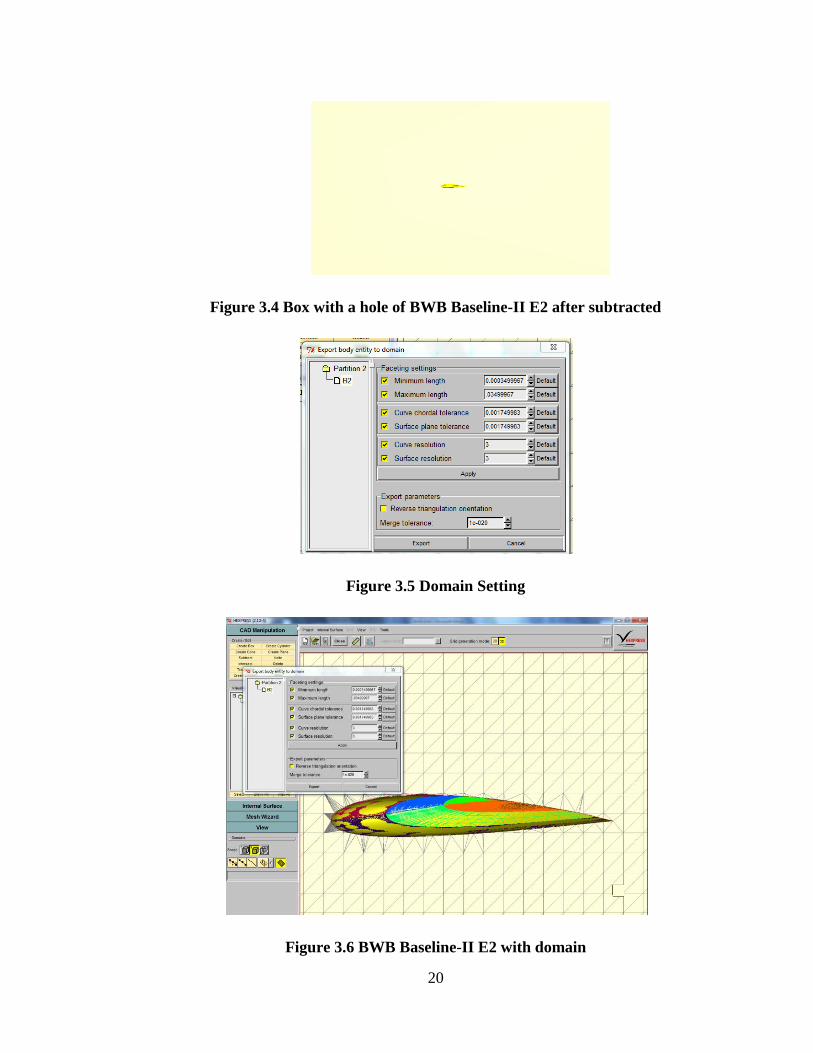
20

Figure 3.4 Box with a hole of BWB Baseline-II E2 after subtracted

Figure 3.5 Domain Setting

Figure 3.6 BWB Baseline-II E2 with domain

21

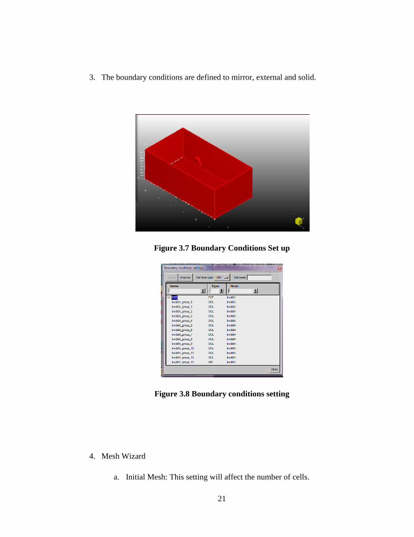
3. The boundary conditions are defined to mirror, external and solid.

Figure 3.7 Boundary Conditions Set up

Figure 3.8 Boundary conditions setting

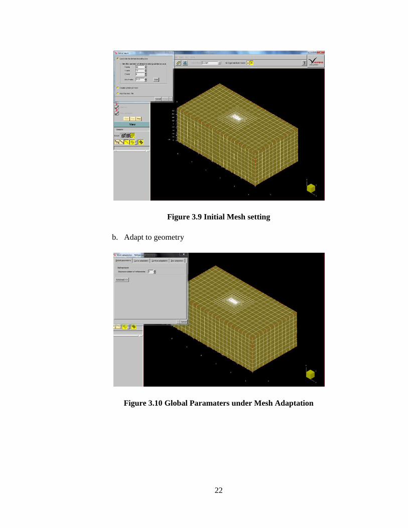
4. Mesh Wizard

a. Initial Mesh: This setting will affect the number of cells.

22

Figure 3.9 Initial Mesh setting

b. Adapt to geometry

Figure 3.10 Global Paramaters under Mesh Adaptation

23

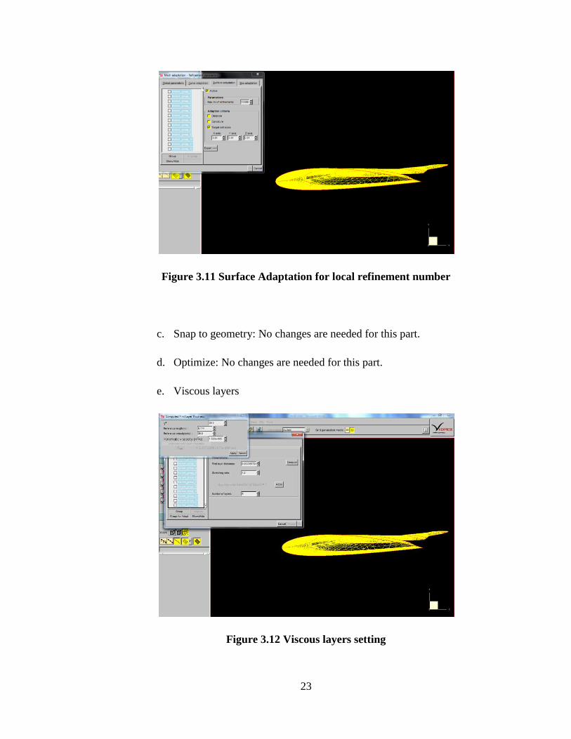
Figure 3.11 Surface Adaptation for local refinement number

c. Snap to geometry: No changes are needed for this part.

d. Optimize: No changes are needed for this part.

e. Viscous layers

Figure 3.12 Viscous layers setting

24

Figure 3.13 Finished mesh of BWB

Figure 3.14 Total number of cells

5. The meshing file is saved to .igg file. Meshing program need to be close first to

proceed to HEXSTREAM.

6. The mesh file is loaded automatic in computation program.

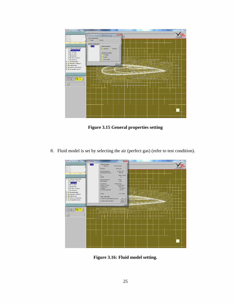
7. The general properties are set.

25

Figure 3.15 General properties setting

8. Fluid model is set by selecting the air (perfect gas) (refer to test condition).

Figure 3.16: Fluid model setting.

26

9. Flow model is set.

Figure 3.17: Flow model parameters

10. No changes are done in solid model, rotating machinery and heat source.

11. The boundary conditions are set according to the information given from

reference.

Table 3.1 Test condition for surrounding

Atmospheric pressure, Patm 100424 Pa

Air temperature, Tair 25°C / 298K (average)

Air density, ρair 1.165 kg/m3

Air kinematic viscosity, νair m2/s

Air velocity, Vair 35 m/s

27

Table 3.2 Test condition for BWB Baseline-II E2

Reference length, Lref 0.114 m

Reference area, Sref 0.03995 m2

Figure 3.18 Boundary conditions setting (solid)

Figure 3.19 Boundary conditions setting (external)

28

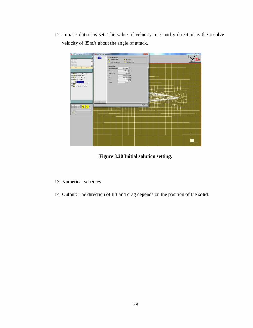
12. Initial solution is set. The value of velocity in x and y direction is the resolve

velocity of 35m/s about the angle of attack.

Figure 3.20 Initial solution setting.

13. Numerical schemes

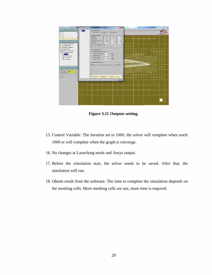
14. Output: The direction of lift and drag depends on the position of the solid.

29

Figure 3.21 Outputs setting.

15. Control Variable: The iteration set to 1000, the solver will complete when reach

1000 or will complete when the graph is converge.

16. No changes at Launching mode and Ansys output.

17. Before the simulation start, the solver needs to be saved. After that, the

simulation will run.

18. Obtain result from the software. The time to complete the simulation depends on

the meshing cells. More meshing cells are use, more time is required.

30

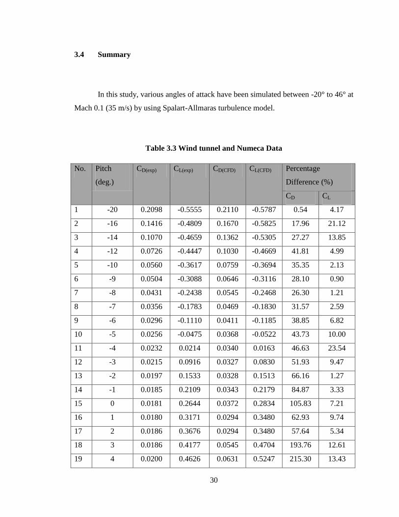
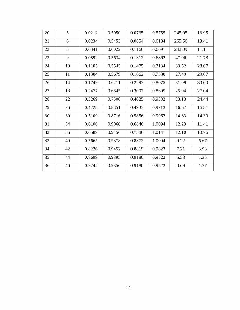
3.4 Summary

In this study, various angles of attack have been simulated between -20° to 46° at

Mach 0.1 (35 m/s) by using Spalart-Allmaras turbulence model.

Table 3.3 Wind tunnel and Numeca Data

No. Pitch

(deg.)

CD(exp) CL(exp) CD(CFD) CL(CFD) Percentage

Difference (%)

CD CL

1 -20 0.2098 -0.5555 0.2110 -0.5787 0.54 4.17

2 -16 0.1416 -0.4809 0.1670 -0.5825 17.96 21.12

3 -14 0.1070 -0.4659 0.1362 -0.5305 27.27 13.85

4 -12 0.0726 -0.4447 0.1030 -0.4669 41.81 4.99

5 -10 0.0560 -0.3617 0.0759 -0.3694 35.35 2.13

6 -9 0.0504 -0.3088 0.0646 -0.3116 28.10 0.90

7 -8 0.0431 -0.2438 0.0545 -0.2468 26.30 1.21

8 -7 0.0356 -0.1783 0.0469 -0.1830 31.57 2.59

9 -6 0.0296 -0.1110 0.0411 -0.1185 38.85 6.82

10 -5 0.0256 -0.0475 0.0368 -0.0522 43.73 10.00

11 -4 0.0232 0.0214 0.0340 0.0163 46.63 23.54

12 -3 0.0215 0.0916 0.0327 0.0830 51.93 9.47

13 -2 0.0197 0.1533 0.0328 0.1513 66.16 1.27

14 -1 0.0185 0.2109 0.0343 0.2179 84.87 3.33

15 0 0.0181 0.2644 0.0372 0.2834 105.83 7.21

16 1 0.0180 0.3171 0.0294 0.3480 62.93 9.74

17 2 0.0186 0.3676 0.0294 0.3480 57.64 5.34

18 3 0.0186 0.4177 0.0545 0.4704 193.76 12.61

19 4 0.0200 0.4626 0.0631 0.5247 215.30 13.43

31

20 5 0.0212 0.5050 0.0735 0.5755 245.95 13.95

21 6 0.0234 0.5453 0.0854 0.6184 265.56 13.41

22 8 0.0341 0.6022 0.1166 0.6691 242.09 11.11

23 9 0.0892 0.5634 0.1312 0.6862 47.06 21.78

24 10 0.1105 0.5545 0.1475 0.7134 33.52 28.67

25 11 0.1304 0.5679 0.1662 0.7330 27.49 29.07

26 14 0.1749 0.6211 0.2293 0.8075 31.09 30.00

27 18 0.2477 0.6845 0.3097 0.8695 25.04 27.04

28 22 0.3269 0.7500 0.4025 0.9332 23.13 24.44

29 26 0.4228 0.8351 0.4933 0.9713 16.67 16.31

30 30 0.5109 0.8716 0.5856 0.9962 14.63 14.30

31 34 0.6100 0.9060 0.6846 1.0094 12.23 11.41

32 36 0.6589 0.9156 0.7386 1.0141 12.10 10.76

33 40 0.7665 0.9378 0.8372 1.0004 9.22 6.67

34 42 0.8226 0.9452 0.8819 0.9823 7.21 3.93

35 44 0.8699 0.9395 0.9180 0.9522 5.53 1.35

36 46 0.9244 0.9356 0.9180 0.9522 0.69 1.77

32

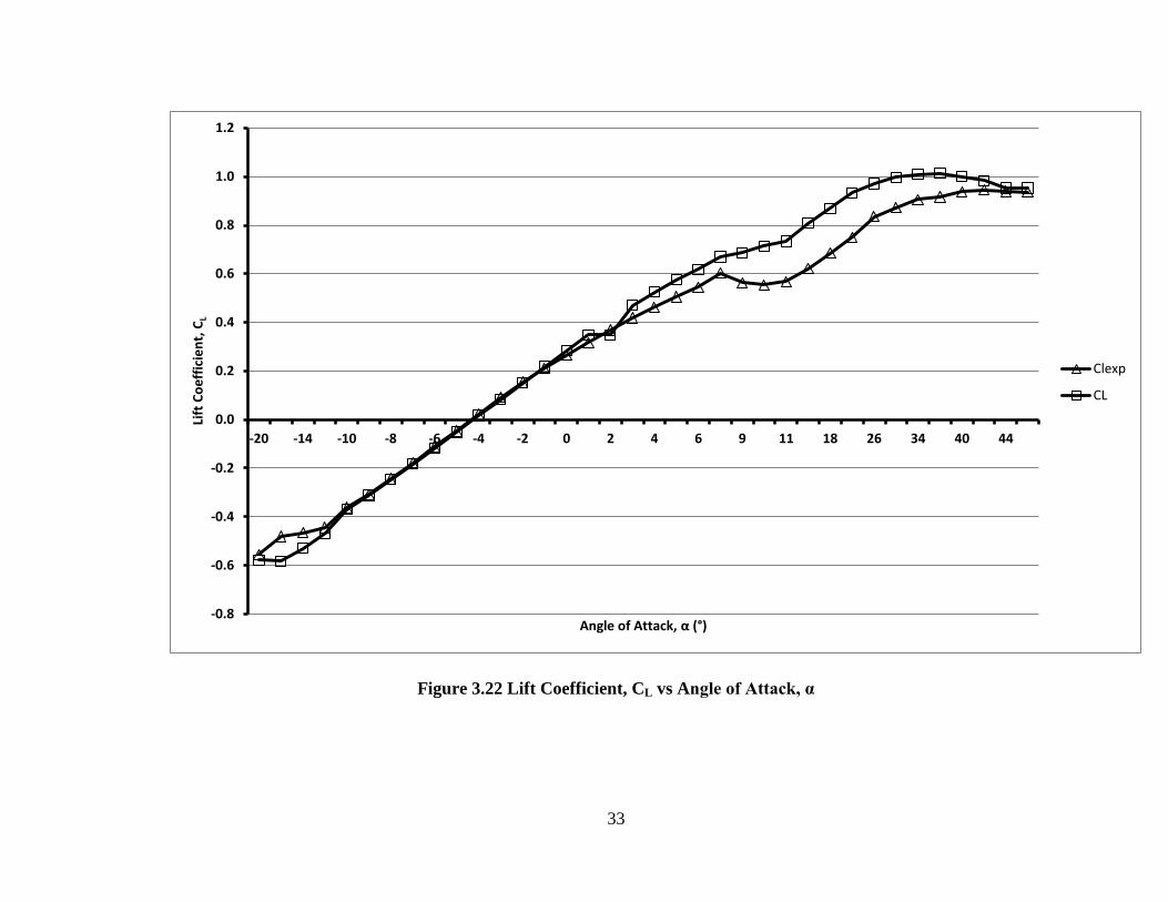
1. Lift Coefficient, CL analysis

From Figure 3.22, it shows the comparison result between CFD simulation and

experimental data for BWB Baseline-II E2. The lift curves show a trend that are similar

to the linear region (α = -10° to 8°) although at α = 2°, there is a slight drop since the

percentage of error at that specific angle of attack is 5.34% which is approaching the

experimental data. However, at α = 3° the percentage of error increased to 12.61% and it

continue to increase linearly till α = 8°. The graph has a curve that is slightly similar to

the experimental result. At α = 44° and 46°, the value of lift coefficient is nearly as the

experimental result with percentage of error 1.35% and 1.77% respectively.

2. Drag Coefficient, CD analysis

As shown in Figure 3.23, the graph of CFD simulation shows a trend

line that is roughly similar to the data obtained from wind tunnel test. The trend

line moves nearly to the experimental data. However, at α = 3°, the line moves

away from the experimental data with the increasing percentage of error. At

α = 9°, the line moves along the experimental data with a significant distance

separating them. The data from CFD simulation is almost the same with the

experimental data at α = 46° with its percentage of error 0.64%.

33

Figure 3.22 Lift Coefficient, CL vs Angle of Attack, α

-0.8

-0.6

-0.4

-0.2

0.0

0.2

0.4

0.6

0.8

1.0

1.2

-20 -14 -10 -8 -6 -4 -2 0 2 4 6 9 11 18 26 34 40 44

Lift

Co

eff

icie

nt,

CL

Angle of Attack, α (°)

Clexp

CL

34

Figure 3.23: Drag Coefficient, CD vs Angle of Attack, α

0.0

0.1

0.2

0.3

0.4

0.5

0.6

0.7

0.8

0.9

1.0

-20 -14 -10 -8 -6 -4 -2 0 2 4 6 9 11 18 26 34 40 44

Dra

g C

oe

ffic

ien

t, C

D

Angle of Attack, α (°)

Cdexp

CD

35

The investigation on aerodynamic characteristics data obtained from CFD

simulation and wind tunnel test, shows that the curve of the graph for both lift and

drag coefficient are slightly similar to each other although there is a signicant

percentage of error with 30% of error at α = 14° for lift coefficient and 265% of error

at α = 6° for drag coefficient. The smallest percentage of error for lift coefficient is

0.9% at α = -9° as for drag coefficient, 0.54% of error at α = -20°.

36

CHAPTER IV

4. GRID SENSITIVITY STUDY

Proceeding from the Parameter Validation, the next chapter is to carry out the

Grid Sensitivity study. Grid Sensitivity study is the stage of obtaining the most

suitable parameter setting that will be use for the simulation using NUMECA. In

order to proceed with this stage, some parameters will be taken into account that will

be vary accordingly to obtain the most suitable parameter setting to be use for the

BWB Baseline-II E5-8 CFD Simulation purposes.

37

CFD Analysis with variation

of grid sensitivity

Independence

achieved?

NO

YES

GRID SENSITIVITY STUDY

STUDY

BWB Baseline-II E5-8

CFD Simulation

Parameter Validation

Obtain BWB-Baseline II E5-8

CAD Drawing

START

Literature review

38

4.1 BWB Baseline-II E5 CAD Drawing

The CAD drawing of the BWB Baseline-II E5 and rectangular canard with

aspect ratio of 8 will be obtained. However, in this chapter, only the drawing of the

half body BWB Baseline-II E5 will be use for the CFD simulation. The drawing of

rectangular canard will be use in the next chapter. The purposes of using the half

body of BWB Baseline-II E5 are to reduce the simulation time by reducing the

computer’s memory usage and saving time in modeling [19].

4.2 CFD Analysis with Variation of Grid Sensitivity

The drawing of the half body BWB Baseline-II E5 is then import to CFD to

generate the meshing. The analysis will be done by varying the values for selected

parameters to obtain a fine mesh and to test the CL, CD and L/D ratio. The process

will stop when the CL, CD, and L/D is approaching to constant at certain number of

grid.

There are mainly four parameters that will be vary to obtain the most suitable

parameter settings which are, (1) Box; (2) Initial Mesh; (3) Faceting; and (4) Number

of Refinement.

4.2.1 Initial Parameters

In order to run the simulation process for grid sensitivity study, a benchmark

parameter setting will be used. For example, when the parameter for the box is to be

39

vary as to obtain the L/D ratio is approaching to constant number of grid, the other

parameters setting for initial mesh, faceting and number of refinement will be based

on the benchmark parameters.

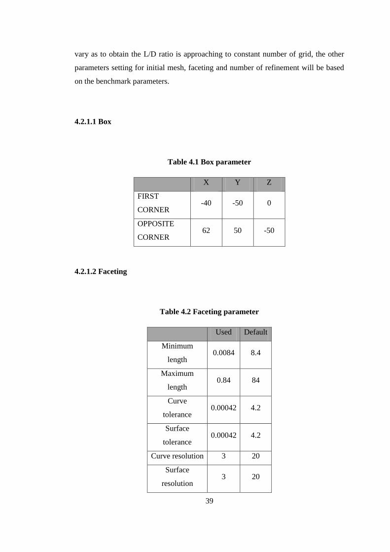
4.2.1.1 Box

Table 4.1 Box parameter

X Y Z

FIRST

CORNER -40 -50 0

OPPOSITE

CORNER 62 50 -50

4.2.1.2 Faceting

Table 4.2 Faceting parameter

Used Default

Minimum

length 0.0084 8.4

Maximum

length 0.84 84

Curve

tolerance 0.00042 4.2

Surface

tolerance 0.00042 4.2

Curve resolution 3 20

Surface

resolution 3 20

40

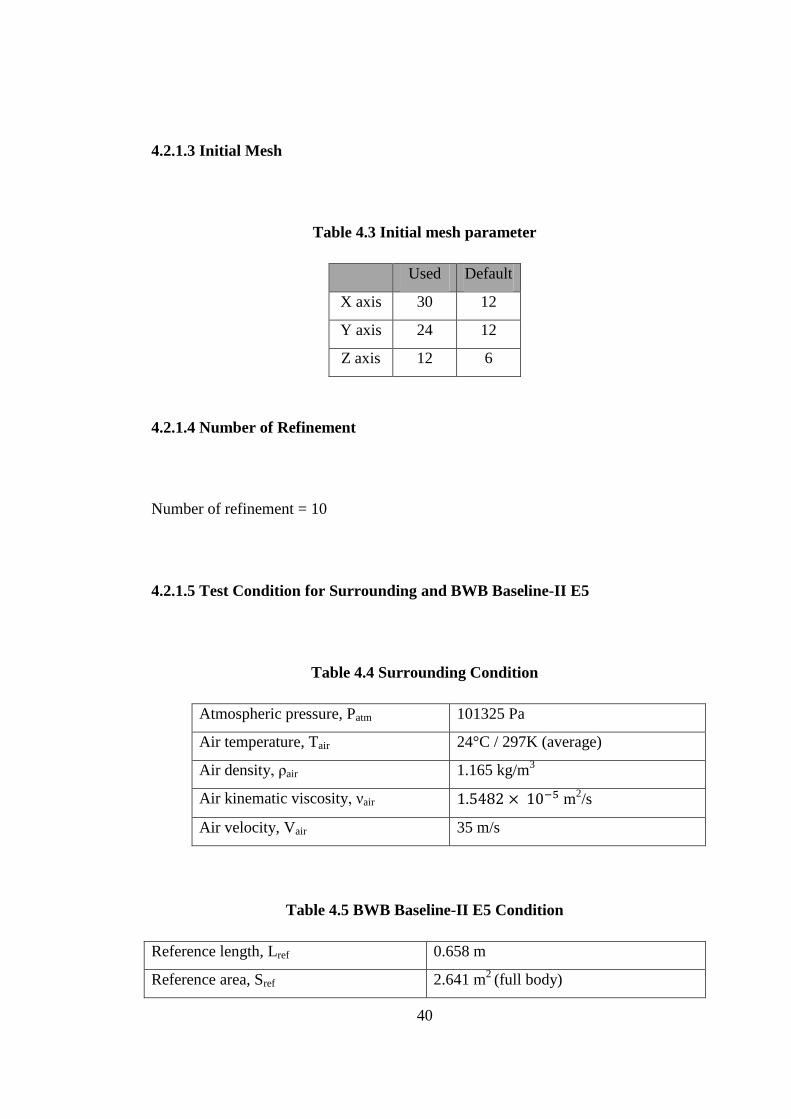
4.2.1.3 Initial Mesh

Table 4.3 Initial mesh parameter

Used Default

X axis 30 12

Y axis 24 12

Z axis 12 6

4.2.1.4 Number of Refinement

Number of refinement = 10

4.2.1.5 Test Condition for Surrounding and BWB Baseline-II E5

Table 4.4 Surrounding Condition

Atmospheric pressure, Patm 101325 Pa

Air temperature, Tair 24°C / 297K (average)

Air density, ρair 1.165 kg/m3

Air kinematic viscosity, νair m2/s

Air velocity, Vair 35 m/s

Table 4.5 BWB Baseline-II E5 Condition

Reference length, Lref 0.658 m

Reference area, Sref 2.641 m2

(full body)

41

Reference volumic mass, ρref 1.1642 kg/m3

4.2.2 Grid Sensitivity Analysis

From the above parameters, the simulation for the grid sensitivity study can

proceed by running simulation for various types of setting.

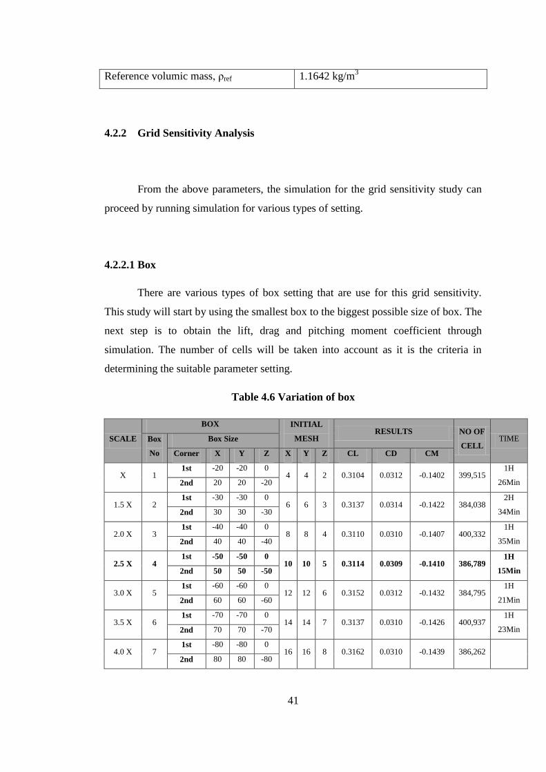
4.2.2.1 Box

There are various types of box setting that are use for this grid sensitivity.

This study will start by using the smallest box to the biggest possible size of box. The

next step is to obtain the lift, drag and pitching moment coefficient through

simulation. The number of cells will be taken into account as it is the criteria in

determining the suitable parameter setting.

Table 4.6 Variation of box

SCALE

BOX INITIAL

MESH RESULTS NO OF

CELL TIME Box

No

Box Size

Corner X Y Z X Y Z CL CD CM

X 1 1st -20 -20 0

4 4 2 0.3104 0.0312 -0.1402 399,515 1H

26Min 2nd 20 20 -20

1.5 X 2 1st -30 -30 0

6 6 3 0.3137 0.0314 -0.1422 384,038 2H

34Min 2nd 30 30 -30

2.0 X 3 1st -40 -40 0

8 8 4 0.3110 0.0310 -0.1407 400,332 1H

35Min 2nd 40 40 -40

2.5 X 4 1st -50 -50 0

10 10 5 0.3114 0.0309 -0.1410 386,789 1H

15Min 2nd 50 50 -50

3.0 X 5 1st -60 -60 0

12 12 6 0.3152 0.0312 -0.1432 384,795 1H

21Min 2nd 60 60 -60

3.5 X 6 1st -70 -70 0

14 14 7 0.3137 0.0310 -0.1426 400,937 1H

23Min 2nd 70 70 -70

4.0 X 7 1st -80 -80 0

16 16 8 0.3162 0.0310 -0.1439 386,262 2nd 80 80 -80

42

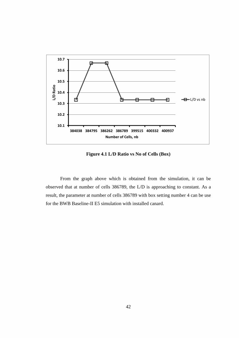
Figure 4.1 L/D Ratio vs No of Cells (Box)

From the graph above which is obtained from the simulation, it can be

observed that at number of cells 386789, the L/D is approaching to constant. As a

result, the parameter at number of cells 386789 with box setting number 4 can be use

for the BWB Baseline-II E5 simulation with installed canard.

10.1

10.2

10.3

10.4

10.5

10.6

10.7

384038 384795 386262 386789 399515 400332 400937

L/D

Rat

io

Number of Cells, nb

L/D vs nb

43

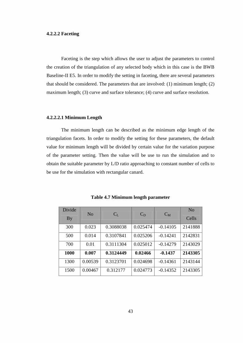
4.2.2.2 Faceting

Faceting is the step which allows the user to adjust the parameters to control

the creation of the triangulation of any selected body which in this case is the BWB

Baseline-II E5. In order to modify the setting in faceting, there are several parameters

that should be considered. The parameters that are involved: (1) minimum length; (2)

maximum length; (3) curve and surface tolerance; (4) curve and surface resolution.

4.2.2.2.1 Minimum Length

The minimum length can be described as the minimum edge length of the

triangulation facets. In order to modify the setting for these parameters, the default

value for minimum length will be divided by certain value for the variation purpose

of the parameter setting. Then the value will be use to run the simulation and to

obtain the suitable parameter by L/D ratio approaching to constant number of cells to

be use for the simulation with rectangular canard.

Table 4.7 Minimum length parameter

Divide

By No CL CD CM

No

Cells

300 0.023 0.3088038 0.025474 -0.14105 2141888

500 0.014 0.3107841 0.025206 -0.14241 2142831

700 0.01 0.3111304 0.025012 -0.14279 2143029

1000 0.007 0.3124449 0.02466 -0.1437 2143305

1300 0.00539 0.3123701 0.024698 -0.14361 2143144

1500 0.00467 0.312177 0.024773 -0.14352 2143305

44

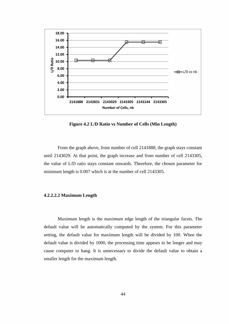
Figure 4.2 L/D Ratio vs Number of Cells (Min Length)

From the graph above, from number of cell 2141888, the graph stays constant

until 2143029. At that point, the graph increase and from number of cell 2143305,

the value of L/D ratio stays constant onwards. Therefore, the chosen parameter for

minimum length is 0.007 which is at the number of cell 2143305.

4.2.2.2.2 Maximum Length

Maximum length is the maximum edge length of the triangular facets. The

default value will be automatically computed by the system. For this parameter

setting, the default value for maximum length will be divided by 100. When the

default value is divided by 1000, the processing time appears to be longer and may

cause computer to hang. It is unnecessary to divide the default value to obtain a

smaller length for the maximum length.

0.00

2.00

4.00

6.00

8.00

10.00

12.00

14.00

16.00

18.00

2141888 2142831 2143029 2143305 2143144 2143305

L/D

Rat

io

Number of Cells, nb

L/D vs nb

45

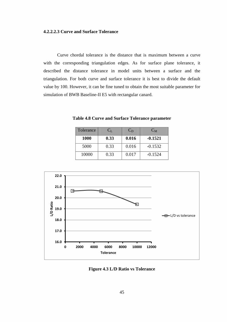
4.2.2.2.3 Curve and Surface Tolerance

Curve chordal tolerance is the distance that is maximum between a curve

with the corresponding triangulation edges. As for surface plane tolerance, it

described the distance tolerance in model units between a surface and the

triangulation. For both curve and surface tolerance it is best to divide the default

value by 100. However, it can be fine tuned to obtain the most suitable parameter for

simulation of BWB Baseline-II E5 with rectangular canard.

Table 4.8 Curve and Surface Tolerance parameter

Tolerance CL CD CM

1000 0.33 0.016 -0.1521

5000 0.33 0.016 -0.1532

10000 0.33 0.017 -0.1524

Figure 4.3 L/D Ratio vs Tolerance

16.0

17.0

18.0

19.0

20.0

21.0

22.0

0 2000 4000 6000 8000 10000 12000

L/D

Rat

io

Tolerance

L/D vs tolerance

46

From the graph of L/D ratio against tolerance above, the value of L/D can be

observed constant at tolerance 1000 until 5000. However, this value drops at

tolerance 10000. Therefore, the most suitable parameter to be use can be determined

at tolerance 1000.

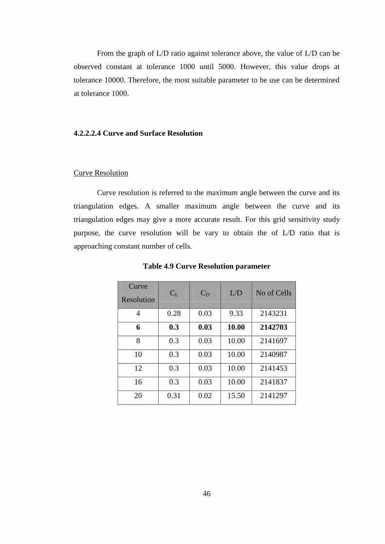
4.2.2.2.4 Curve and Surface Resolution

Curve Resolution

Curve resolution is referred to the maximum angle between the curve and its

triangulation edges. A smaller maximum angle between the curve and its

triangulation edges may give a more accurate result. For this grid sensitivity study

purpose, the curve resolution will be vary to obtain the of L/D ratio that is

approaching constant number of cells.

Table 4.9 Curve Resolution parameter

Curve

Resolution CL CD L/D No of Cells

4 0.28 0.03 9.33 2143231

6 0.3 0.03 10.00 2142703

8 0.3 0.03 10.00 2141697

10 0.3 0.03 10.00 2140987

12 0.3 0.03 10.00 2141453

16 0.3 0.03 10.00 2141837

20 0.31 0.02 15.50 2141297

47

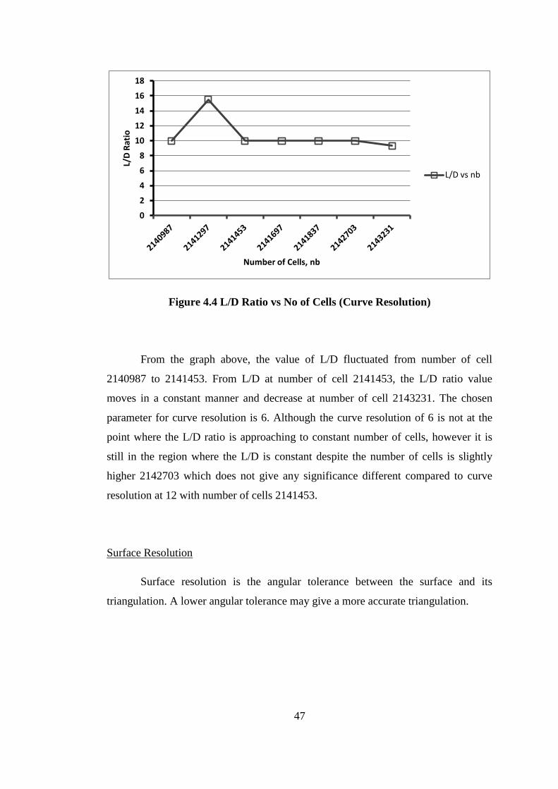
Figure 4.4 L/D Ratio vs No of Cells (Curve Resolution)

From the graph above, the value of L/D fluctuated from number of cell

2140987 to 2141453. From L/D at number of cell 2141453, the L/D ratio value

moves in a constant manner and decrease at number of cell 2143231. The chosen

parameter for curve resolution is 6. Although the curve resolution of 6 is not at the

point where the L/D ratio is approaching to constant number of cells, however it is

still in the region where the L/D is constant despite the number of cells is slightly

higher 2142703 which does not give any significance different compared to curve

resolution at 12 with number of cells 2141453.

Surface Resolution

Surface resolution is the angular tolerance between the surface and its

triangulation. A lower angular tolerance may give a more accurate triangulation.

0

2

4

6

8

10

12

14

16

18

L/D

Rat

io

Number of Cells, nb

L/D vs nb

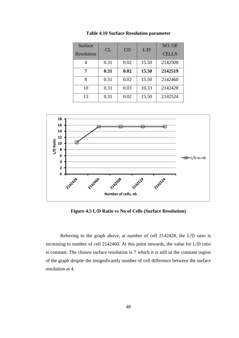
48

Table 4.10 Surface Resolution parameter

Surface

Resolution CL CD L/D

NO. OF

CELLS

4 0.31 0.02 15.50 2142508

7 0.31 0.02 15.50 2142519

8 0.31 0.02 15.50 2142460

10 0.31 0.03 10.33 2142428

13 0.31 0.02 15.50 2142524

Figure 4.5 L/D Ratio vs No of Cells (Surface Resolution)

Referring to the graph above, at number of cell 2142428, the L/D ratio is

increasing to number of cell 2142460. At this point onwards, the value for L/D ratio

is constant. The chosen surface resolution is 7 which it is still in the constant region

of the graph despite the insignificantly number of cell difference between the surface

resolution at 4.

0

2

4

6

8

10

12

14

16

18

L/D

Rat

io

Number of cells, nb

L/D vs nb

49

4.2.2.3 Initial Mesh

The initial mesh is the crucial part that gives a large effect to the number of

cells. As the number of mesh increases, the number of cells will also increase.

Therefore, in order to obtain a lower number of cells in order to save time during

meshing, the number of mesh should be lower. With a higher number of cells, the

mesh quality would be finer.

Table 4.11 Initial Mesh parameter

Mesh CL CD L/D No. of

Cells

Mesh 1 0.3265 0.0164 19.97 1080

Mesh 2 0.3243 0.0163 19.94 2560

Mesh 3 0.3271 0.0170 19.21 5000

Mesh 4 0.3266 0.0163 19.98 8640

Mesh 5 0.3250 0.0159 20.47 13720

Mesh 6 0.3242 0.0163 19.84 20480

Mesh 7 0.3251 0.0154 21.05 29160

Mesh 8 0.3270 0.0170 19.18 40000

Mesh 9 0.3270 0.0166 19.75 53240

Mesh 10 0.3268 0.0164 19.97 69120

Table 4.12 Types of Initial Mesh

Mesh

1

Mesh

2

Mesh

3

Mesh

4

Mesh

5

Mesh

6

Mesh

7

Mesh

8

Mesh

9

Mesh

10

X axis 15 20 25 30 35 40 45 50 55 60

Y axis 12 16 20 24 28 32 36 40 44 48

Z axis 6 8 10 12 14 16 18 20 22 24

50

Figure 4.6 L/D Ratio vs No of Cells (Initial Mesh)

Graph above shows L/D ratio against number of cells. It can be observed that

the graph is fluctuating until at number of cell 40000, the L/D ratio is approaching to

constant number of cells. At this point, the parameter to be use for simulation of

BWB Baseline-II E5 with rectangular canard can be determined.

4.2.2.4 Number of Refinement

The number of refinement is use to adjust the quality of the mesh. A higher

number of refinements, the quality of the mesh will be finer. However, when the

number of the refinement increase, the number of cells will also increase.

Table 4.13 Number of Refinement parameter

No of

Refinement CL CD CM

No. of

Cells L/D

7 0.3173 0.0392 -0.1436 222772 8.09

15.9

16

16.1

16.2

16.3

16.4

16.5

16.6

0 20000 40000 60000 80000

L/D

Rat

io

Number of Cells, nb

L/D vs nb

51

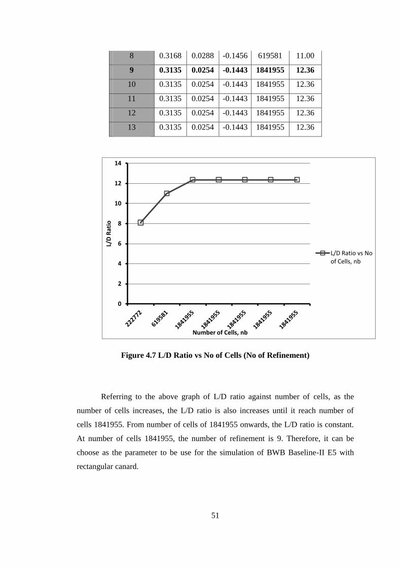
8 0.3168 0.0288 -0.1456 619581 11.00

9 0.3135 0.0254 -0.1443 1841955 12.36

10 0.3135 0.0254 -0.1443 1841955 12.36

11 0.3135 0.0254 -0.1443 1841955 12.36

12 0.3135 0.0254 -0.1443 1841955 12.36

13 0.3135 0.0254 -0.1443 1841955 12.36

Figure 4.7 L/D Ratio vs No of Cells (No of Refinement)

Referring to the above graph of L/D ratio against number of cells, as the

number of cells increases, the L/D ratio is also increases until it reach number of

cells 1841955. From number of cells of 1841955 onwards, the L/D ratio is constant.

At number of cells 1841955, the number of refinement is 9. Therefore, it can be

choose as the parameter to be use for the simulation of BWB Baseline-II E5 with

rectangular canard.

0

2

4

6

8

10

12

14

L/D

Rat

io

Number of Cells, nb

L/D Ratio vs No of Cells, nb

52

4.3 Final Parameter Settings

After running the simulation for the grid sensitivity study, it can be come to a

consideration for the parameter setting that will be use for the simulation of BWB

Baseline-II E5 with a rectangular canard which will be use in the next chapter.

4.3.1 Box

Table 4.14 Box parameter

PARAMETER VALUE

X Y Z

FIRST CORNER -50 0 -50

OPPOSITE

CORNER 50 50 50

4.3.2 Faceting

Table 4.15 Faceting parameter

PARAMETER VALUE

min length 0.007

max length /100

curve tolerance /1000

surface tolerance /1000

curve resolution 6

surface resolution 7

53

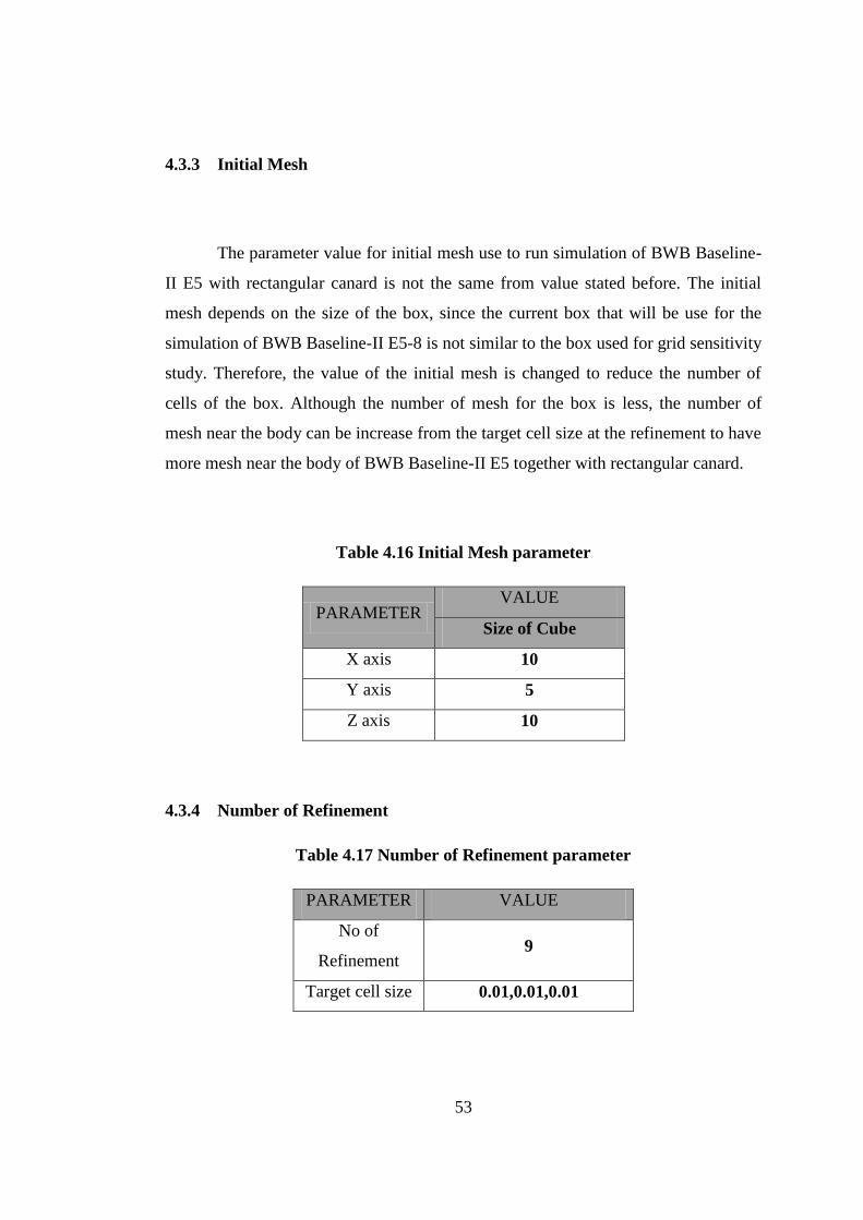
4.3.3 Initial Mesh

The parameter value for initial mesh use to run simulation of BWB Baseline-

II E5 with rectangular canard is not the same from value stated before. The initial

mesh depends on the size of the box, since the current box that will be use for the

simulation of BWB Baseline-II E5-8 is not similar to the box used for grid sensitivity

study. Therefore, the value of the initial mesh is changed to reduce the number of

cells of the box. Although the number of mesh for the box is less, the number of

mesh near the body can be increase from the target cell size at the refinement to have

more mesh near the body of BWB Baseline-II E5 together with rectangular canard.

Table 4.16 Initial Mesh parameter

PARAMETER VALUE

Size of Cube

X axis 10

Y axis 5

Z axis 10

4.3.4 Number of Refinement

Table 4.17 Number of Refinement parameter

PARAMETER VALUE

No of

Refinement 9

Target cell size 0.01,0.01,0.01

54

CHAPTER V

5. RESULT AND DISCUSSION

This chapter will discuss the result that is obtained from the simulation of the

BWB Baseline-II E5-8 with rectangular canard aspect ratio of 8 at various canard

setting angles, δ, at angle of attack, α = 10° by using the steps and parameters as

mentioned in the previous chapter.

The obtained data will be tabled and the graph of lift, drag and pitching

moment coefficient (CL, CD, and CM) will be plotted against the canard setting angle.

The aerodynamic characteristics from the result will be discuss by taking into

account the pressure and Mach contour as well as the velocity vectors.

55

5.1 Aerodynamic Analysis for BWB Baseline-II E5-8

The simulation process for BWB Baseline-II E5-8 is done at angle of attack

10° with various canard setting angles. For this project purposes, the deflection

angles of canard is taken from δ = -22° to δ = 8°. From the collected data, the lift,

drag and pitching moment coefficient (CL, CD and CM) of the BWB Baseline-II E5-8

can be discussed.

5.1.1 Result of BWB Baseline-II E5-8 CFD Simulation

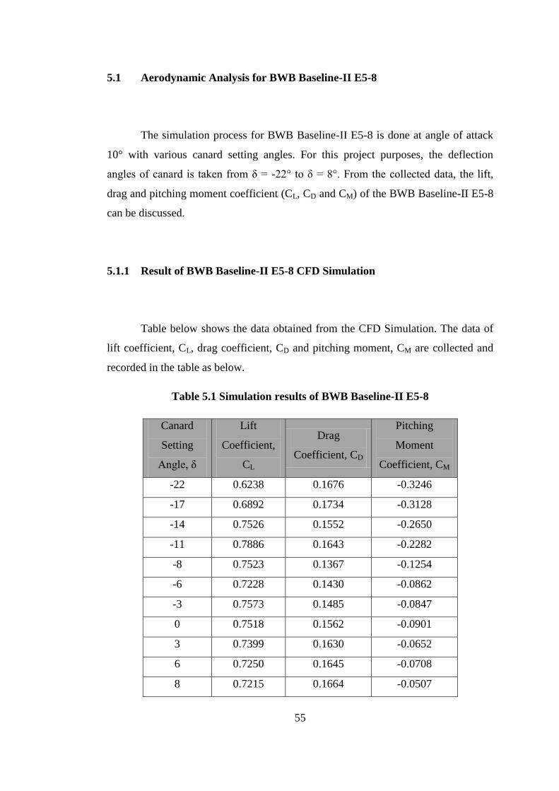
Table below shows the data obtained from the CFD Simulation. The data of

lift coefficient, CL, drag coefficient, CD and pitching moment, CM are collected and

recorded in the table as below.

Table 5.1 Simulation results of BWB Baseline-II E5-8

Canard

Setting

Angle, δ

Lift

Coefficient,

CL

Drag

Coefficient, CD

Pitching

Moment

Coefficient, CM

-22 0.6238 0.1676 -0.3246

-17 0.6892 0.1734 -0.3128

-14 0.7526 0.1552 -0.2650

-11 0.7886 0.1643 -0.2282

-8 0.7523 0.1367 -0.1254

-6 0.7228 0.1430 -0.0862

-3 0.7573 0.1485 -0.0847

0 0.7518 0.1562 -0.0901

3 0.7399 0.1630 -0.0652

6 0.7250 0.1645 -0.0708

8 0.7215 0.1664 -0.0507

56

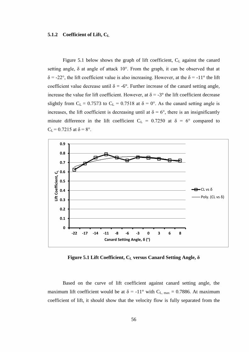
5.1.2 Coefficient of Lift, CL

Figure 5.1 below shows the graph of lift coefficient, CL against the canard

setting angle, δ at angle of attack 10°. From the graph, it can be observed that at

δ = -22°, the lift coefficient value is also increasing. However, at the δ = -11° the lift

coefficient value decrease until δ = -6°. Further increase of the canard setting angle,

increase the value for lift coefficient. However, at δ = -3° the lift coefficient decrease

slightly from CL = 0.7573 to CL = 0.7518 at δ = 0°. As the canard setting angle is

increases, the lift coefficient is decreasing until at δ = 6°, there is an insignificantly

minute difference in the lift coefficient CL = 0.7250 at δ = 6° compared to

CL = 0.7215 at δ = 8°.

Figure 5.1 Lift Coefficient, CL versus Canard Setting Angle, δ

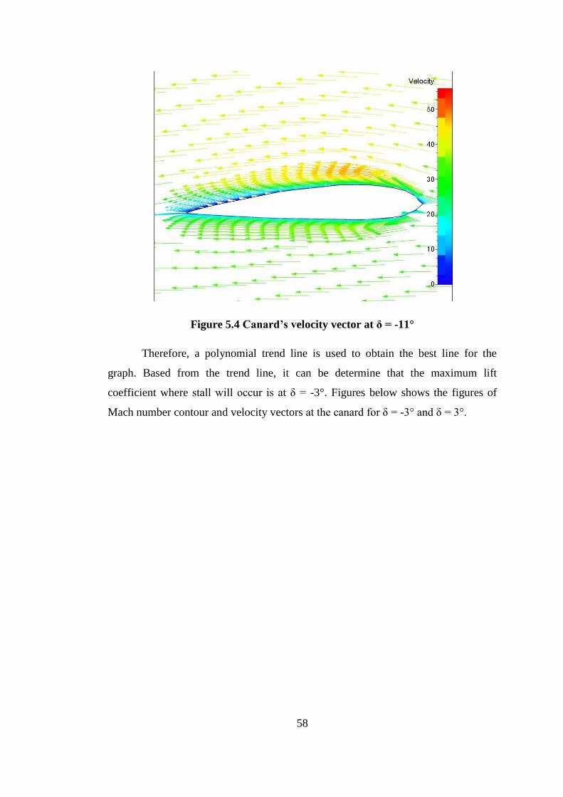
Based on the curve of lift coefficient against canard setting angle, the

maximum lift coefficient would be at δ = -11° with CL, max = 0.7886. At maximum

coefficient of lift, it should show that the velocity flow is fully separated from the

0

0.1

0.2

0.3

0.4

0.5

0.6

0.7

0.8

0.9

-22 -17 -14 -11 -8 -6 -3 0 3 6 8

Lift

Co

eff

icie

nt,

CL

Canard Setting Angle, δ (°)

CL vs δ

Poly. (CL vs δ)

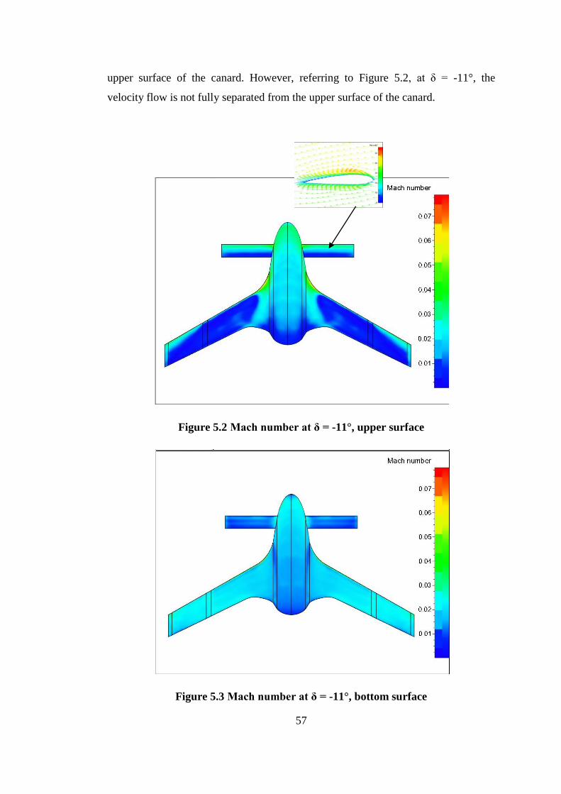
57

upper surface of the canard. However, referring to Figure 5.2, at δ = -11°, the

velocity flow is not fully separated from the upper surface of the canard.

Figure 5.2 Mach number at δ = -11°, upper surface

Figure 5.3 Mach number at δ = -11°, bottom surface

58

Figure 5.4 Canard’s velocity vector at δ = -11°

Therefore, a polynomial trend line is used to obtain the best line for the

graph. Based from the trend line, it can be determine that the maximum lift

coefficient where stall will occur is at δ = -3°. Figures below shows the figures of

Mach number contour and velocity vectors at the canard for δ = -3° and δ = 3°.

59

Figure 5.5 Mach number contour at δ = -3°, upper surface

Figure 5.6 Mach number contour at δ = -3°,bottom surface

60

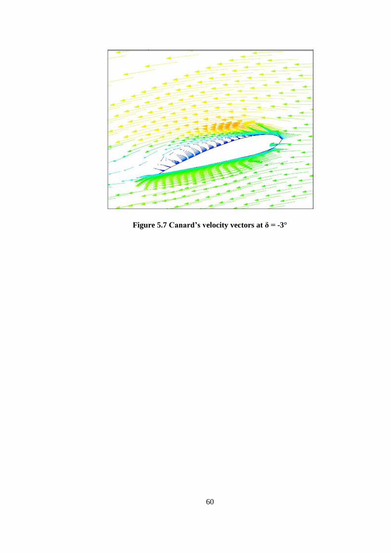
Figure 5.7 Canard’s velocity vectors at δ = -3°

61

Figure 5.8 Mach number contour at δ = 3°, upper surface

Figure 5.9 Mach number contour at δ = 3°, bottom surface

62

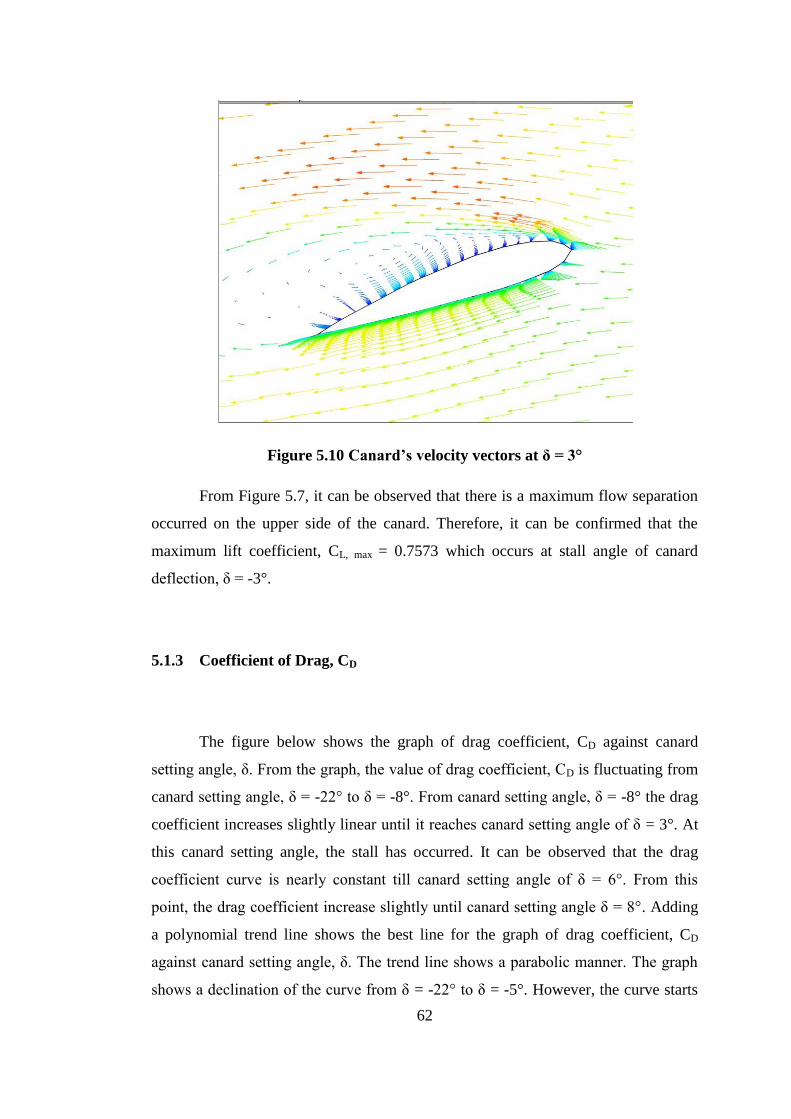
Figure 5.10 Canard’s velocity vectors at δ = 3°

From Figure 5.7, it can be observed that there is a maximum flow separation

occurred on the upper side of the canard. Therefore, it can be confirmed that the

maximum lift coefficient, CL, max = 0.7573 which occurs at stall angle of canard

deflection, δ = -3°.

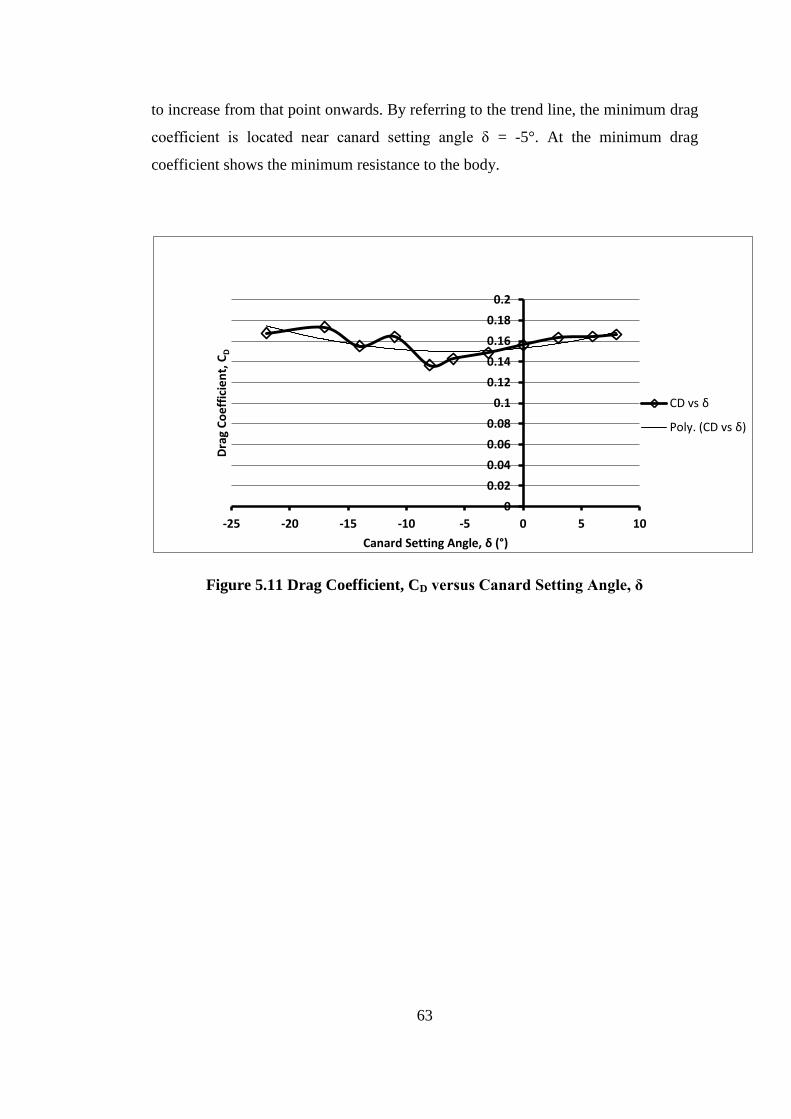
5.1.3 Coefficient of Drag, CD

The figure below shows the graph of drag coefficient, CD against canard

setting angle, δ. From the graph, the value of drag coefficient, CD is fluctuating from

canard setting angle, δ = -22° to δ = -8°. From canard setting angle, δ = -8° the drag

coefficient increases slightly linear until it reaches canard setting angle of δ = 3°. At

this canard setting angle, the stall has occurred. It can be observed that the drag

coefficient curve is nearly constant till canard setting angle of δ = 6°. From this

point, the drag coefficient increase slightly until canard setting angle δ = 8°. Adding

a polynomial trend line shows the best line for the graph of drag coefficient, CD

against canard setting angle, δ. The trend line shows a parabolic manner. The graph

shows a declination of the curve from δ = -22° to δ = -5°. However, the curve starts

63

to increase from that point onwards. By referring to the trend line, the minimum drag

coefficient is located near canard setting angle δ = -5°. At the minimum drag

coefficient shows the minimum resistance to the body.

Figure 5.11 Drag Coefficient, CD versus Canard Setting Angle, δ

0

0.02

0.04

0.06

0.08

0.1

0.12

0.14

0.16

0.18

0.2

-25 -20 -15 -10 -5 0 5 10

Dra

g C

oe

ffic

ien

t, C

D

Canard Setting Angle, δ (°)

CD vs δ

Poly. (CD vs δ)

64

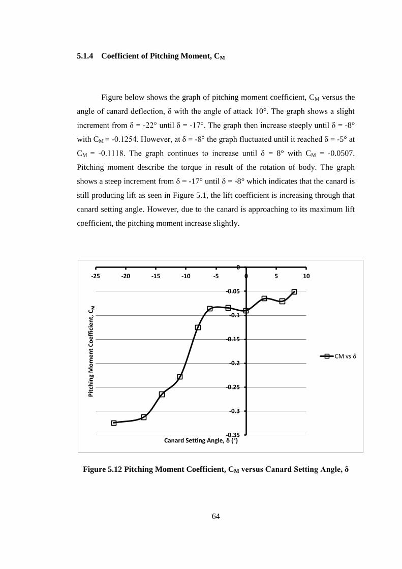
5.1.4 Coefficient of Pitching Moment, CM

Figure below shows the graph of pitching moment coefficient, CM versus the

angle of canard deflection, δ with the angle of attack 10°. The graph shows a slight

increment from δ = -22° until δ = -17°. The graph then increase steeply until δ = -8°

with CM = -0.1254. However, at δ = -8° the graph fluctuated until it reached δ = -5° at

CM = -0.1118. The graph continues to increase until δ = 8° with CM = -0.0507.

Pitching moment describe the torque in result of the rotation of body. The graph

shows a steep increment from δ = -17° until δ = -8° which indicates that the canard is

still producing lift as seen in Figure 5.1, the lift coefficient is increasing through that

canard setting angle. However, due to the canard is approaching to its maximum lift

coefficient, the pitching moment increase slightly.

Figure 5.12 Pitching Moment Coefficient, CM versus Canard Setting Angle, δ

-0.35

-0.3

-0.25

-0.2

-0.15

-0.1

-0.05

0

-25 -20 -15 -10 -5 0 5 10

Pit

chin

g M

om

en

t C

oe

ffic

ien

t, C

M

Canard Setting Angle, δ (°)

CM vs δ

65

5.1.5 Pressure Distribution

From the pressure distribution, when there is a difference in pressure at upper

and lower surface of the body, the body will experience lift.

Figure 5.13 Pressure contours at δ = -11° for upper (left) and lower (right)

surfaces

Figure 5.14 Pressure contours at δ = -5° for upper (left) and lower (right)

surfaces

Figure 5.15 Pressure contours at δ = -3° for upper (left) and lower (right)

surfaces

66

Figure 5.16 Pressure contours at δ = 3° for upper (left) and lower (right)

surfaces

Figure 5.14 shows the pressure contours at δ = -5°. As mentioned previously,

the minimum drag coefficient is at δ = -5°. It can be observed that at δ = -5° the

pressure at the leading edge of wing is less compared to other canard setting angle.

When the pressure is less, the resistance to the wind is also decrease. Since the

resistance is less, the drag is at its minimum.

Figures above show that there is a pressure difference at the upper and lower

surfaces. The pressure at the lower surface is higher than the pressure at the upper

surface. As a result, the lift force is produced due to this difference in pressure

distribution.

67

CHAPTER VI

6.0 CONCLUSION AND RECOMMENDATION

68

6.1 Conclusion

The BWB Baseline-II E5-8 have a maximum lift coefficient, CL, max = 0.7573

at canard setting angle δ = -3°. At this point, the flow separation occurs which result

in stall. From the result obtained, the minimum drag coefficient is located at canard

setting angle δ = -5° with CD = 0.1430.

6.2 Recommendation

There are some improvements that can be done for the future work.

1) Improve mesh quality by using a smaller mesh size to obtain the finest mesh

2) Increase the initial mesh parameter to increase the number of mesh in the

boundary.

3) Upgrade the existing computer in order for it to be able to run simulation of a

body with more number of cells and smaller mesh size.

69

7.0 REFERENCES

1. Robert F. Stengel, “Aircraft Flight Dynamics”, 2008.

2. John P. Fielding, “Introduction to Aircraft Design”, 2008.

3. John D. Anderson, “Introduction to Flight”, 2008.

4. Thomas C. Corke, “Design of Aircraft”. Upper Saddle River, New Jersey:

Pearson/Prentice Hall, 2003.

5. Zurriati M. Ali, Wahyu Kuntjoro, Wirachman Wisnoe, Rizal E. M Nasir.

“The Effect of Canard on Aerodynamics of Blended Wing Body”, Applied

Mechanics and Materials, Trans Tech Publications, Switzerland.

6. http://www.aerospaceweb.org/question/dynamics/q0045.shtml, September 23,

2001.

7. Yunus A.Cengel, John M. Cimbala, “Fluid Mechanics Fundamentals and

Applications”, Singapore, Mc-Graw Hill, 2006.

8. Canards, Evan Neblett, Mike Metheny, Leifur Thor Leifsson, AOE 4124

Configuration Aerodynamics Virginia Tech 17. March 2003.

70

9. M.R. Soltani, F. Askari, A.R. Davari and A. Nayebzadeh. “Effects of Canard

Position on Wing Surface Pressure Transaction” Mechanical Engineering

Vol. 17, No. 2, pp. 136-145, Sharif University of Technology, April 2010.

10. Thomas C. Corke, “Design of Aircraft”. Upper Saddle River, New Jersey:

Pearson/Prentice Hall, 2003.

11. The Blended Wing Body Aircraft Leifur T. Leifsson and William H. Mason

Virginia Polytechnic Institute and State University Blacksburg, VA, USA.

12. N. Qin, A. Vavalle, A Le Moigne, M. Laban, K.Hackett, P. Weinerfelt.

Aerodynamics Studies for Blended Wing Body Aircraft. 9th AIAA/ISSMO

Symposium on Multidisciplinary Analysis and optimization, 4 – 6 September

(2002), Atlanta, Georgia.

13. S. Siouris, N. Qin. Study of the Effects of Wing Sweep on the Aerodynamic

Performance of a Blended Wing Body. (2006) Aerodynamics and

Thermofluids Group, Department of Mechanical Engineering, University of

Sheffield, UK.

14. Wirachman Wisnoe, Wahyu Kuntjoro, Firdaus Mohamad, Rizal Effendy

Mohd Nasir, Nor F Reduan, Zurriati Ali, "Experimental Results Analysis for

UiTM BWB Baseline-I and Baseline-II UAV Running at 0.1 Mach number",

International Journal of Mechanics, Issue 2, Volume 4, 2010, ISSN: 1998-

4448, pp. 23-32.

15. John P. Fielding, “Introduction to Aircraft Design”, 2008.

16. Zurriati M. Ali, Wahyu Kuntjoro, Wirachman Wisnoe, Rizal Efendy M.

Nasir, Firdaus Mohamad, Nor F. Reduan, “The Aerodynamics Performance

of Blended Wing Body Baseline-II E2”, The 2011 International Conference

on Fluid Dynamics and Thermodynamics Technologies (FDTT 2011), Bali,

Indonesia, April 1-3, 2011, ISBN: 978-1-4244-9831-4.

17. http://science.howstuffworks.com/transport/flight/modern/airplanes5.htm

18. http://science.howstuffworks.com/transport/flight/modern/airplanes1.htm

71

19. Zurriati M. Ali, Wahyu Kuntjoro, Wirachman Wisnoe, Rizal Efendy M.

Nasir, Matzaini K., “The Aerodynamic Study of Low Aspect Ratio Canard on

BWB-Baseline II E2”, The 2010 International Conference on Advances in

Mechanical Engineering (ICAME 2010), Faculty of Mechanical Engineering,

UiTM.

72

APPENDICES

APPENDIX A – CAD Drawing of BWB Baseline II E5-8

73

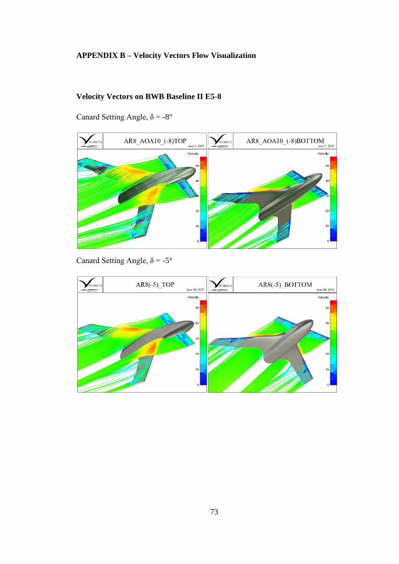
APPENDIX B – Velocity Vectors Flow Visualization

Velocity Vectors on BWB Baseline II E5-8

Canard Setting Angle, δ = -8°

Canard Setting Angle, δ = -5°

74

Canard Setting Angle, δ = -3°

Canard Setting Angle, δ = 0°

Canard Setting Angle, δ = 3°

75

APPENDIX B1 – Velocity Vectors Flow Visualization

Wing’s Velocity Vectors

Canard Setting Angle, δ = -8°

Canard Setting Angle, δ = -5°

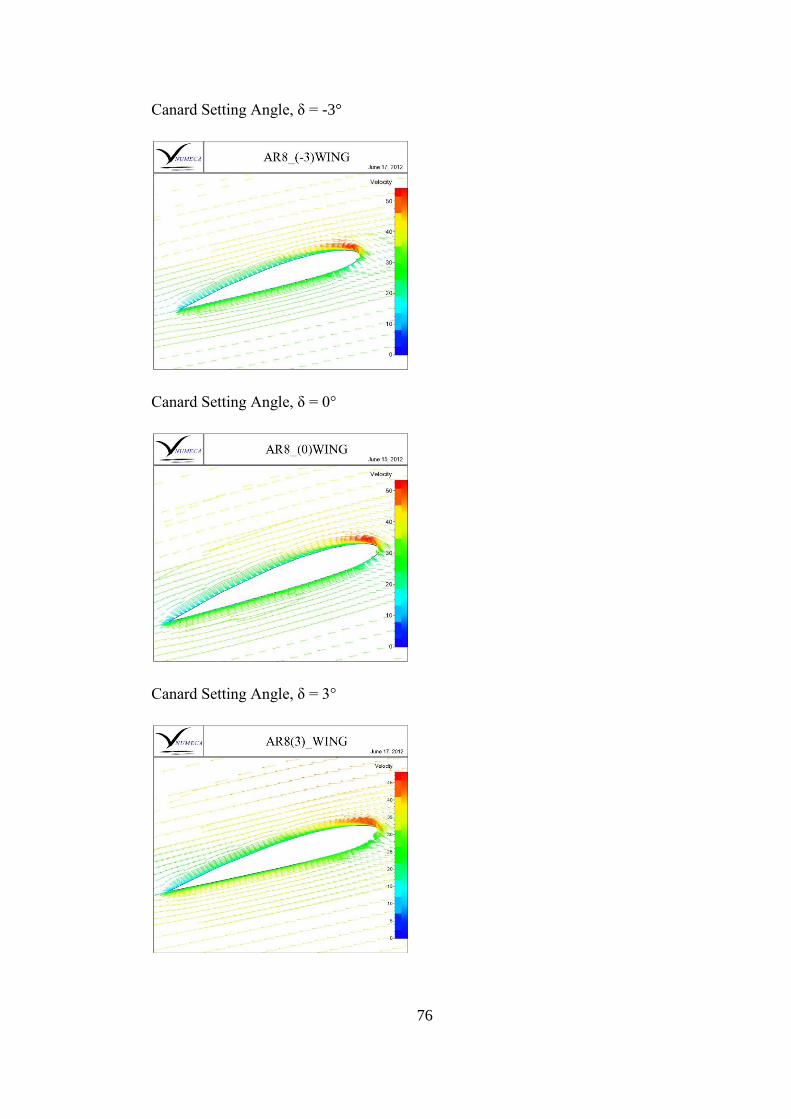
76

Canard Setting Angle, δ = -3°

Canard Setting Angle, δ = 0°

Canard Setting Angle, δ = 3°