final report to the florida department of …swashware.com/flagsim/final report_bdk77-977-18.pdf ·...
TRANSCRIPT

FINAL REPORT
to
THE FLORIDA DEPARTMENT OF TRANSPORTATION RESEARCH CENTER
on Project
“Impact of Lane Closures on Roadway Capacity, Phase 2”
FDOT Contract BDK77-977-18 (UF Project 93879)
January 2014
University of Florida Transportation Research Center
Department of Civil and Coastal Engineering

ii
DISCLAIMER
The contents of this report reflect the views of the authors, who are responsible for the facts and the accuracy of the data published herein. The opinions, findings, and conclusions expressed in this publication are those of the authors and not necessarily those of the State of Florida Department of Transportation.

iii
SI (MODERN METRIC) CONVERSION FACTORS
iv
TECHNICAL REPORT DOCUMENTATION PAGE
1. Report No. 2. Government Accession No. 3. Recipient's Catalog No.
4. Title and Subtitle 5. Report Date
Impact of Lane Closures on Roadway Capacity, Phase 2
January 2014 6. Performing Organization Code
UF-TRC 8. Performing Organization Report No.
7. Author(s) TRC-FDOT-93879-2014 Scott S. Washburn, Donald Watson, and Ziqi Song
9. Performing Organization Name and Address 10. Work Unit No. (TRAIS)
Transportation Research Center University of Florida 512 Weil Hall / P.O. Box 116580 Gainesville, FL 32611-6580
11. Contract or Grant No.
FDOT Contract BDK77-977-18
13. Type of Report and Period Covered 12. Sponsoring Agency Name and Address
Final Report Florida Department of Transportation 605 Suwannee St. MS 30 Tallahassee, Florida 32399 (850) 414 - 4615 14. Sponsoring Agency Code
15. Supplementary Notes
16. Abstract This project is a follow-up to Florida Department of Transportation (FDOT) research project BD545-61, “Impact of Lane Closures on Roadway Capacity” (specifically, Part A: Development of a Two-Lane Work Zone Lane Closure Analysis Procedure and Part C: Modeling Diversion Propensity at Work Zones). In this previous project, the primary objective was to update the procedure in the Plans Preparation Manual (PPM), Volume 1, Section 10.14.7 (2006), for two-lane roadways. Field data collection was not included in the previous project; thus, the results were based strictly on simulation data from the FlagSim simulation program.
The primary objective of this project was to update the two-lane roadway with a lane closure analysis procedure developed under the previous project, based on calibrating the FlagSim simulation program to field data. An additional aspect of this that was not considered in the BD545-61 project was to account for the effect of grade on the work zone performance measures. An additional project objective was to update the RTF estimation method developed under the BD545-61 project, as necessary, based on measured traffic demands (before and during) at work zone field sites.
Field data were collected at three sites and used to calibrate the FlagSim program. FlagSim was then used to generate the data used to update the models contained in the analysis procedure developed under the previous project. Local area traffic demand data were also used to update the RTF estimation model.
17. Key Words 18. Distribution Statement
Work Zones, Work Zone Capacity, Two-Lane Roadways, Lane Closure, Traffic Diversion
No restrictions. This document is available to the public through the National Technical Information Service, Springfield, VA, 22161.
19 Security Classif. (of this report) 20.Security Classif. (of this page) 21.No. of Pages 22 Price
Unclassified Unclassified 135
Form DOT F 1700.7 (8-72) Reproduction of completed page authorized
v
ACKNOWLEDGMENTS
The authors would like to express their sincere appreciation to Mr. Ezzeldin Benghuzzi of the Florida Department of Transportation (Central Office) for the support and guidance he provided on this project. Thanks also to Mr. Scott Hardee of the Florida Department of Transportation for coordinating the local area before- and during-construction traffic counts at the work zone field sites. Thanks also to the numerous people that assisted us with coordinating our data collection efforts in the field.

vi
EXECUTIVE SUMMARY
This project is a follow-up to Florida Department of Transportation (FDOT) research project
BD545-61, “Impact of Lane Closures on Roadway Capacity” (specifically, Part A: Development
of a Two-Lane Work Zone Lane Closure Analysis Procedure and Part C: Modeling Diversion
Propensity at Work Zones). In this previous project, the primary objective was to update the
procedure in the Plans Preparation Manual (PPM), Volume 1, Section 10.14.7 (2006), for two-
lane roadways. Field data collection was not included in the previous project; thus, the results
were based strictly on simulation data from the FlagSim simulation program.
Before the preceding research project, the FDOT developed an analysis procedure for two-
lane roadways with a lane closure that was a relatively simple deterministic procedure, with
rough approximations for work zone capacity and other important parameter values. Through
the previous project (BD545-61), a new analysis procedure was developed that is sensitive to the
major factors that influence work zone performance measures. However, the main limitation
from the BD545-61 project was the lack of field data to use for calibrating the various simulation
parameters.
Another aspect of the BD545-61 project was to develop a method to estimate the amount
of traffic diversion that occurs at a work zone location. The previous analysis procedure in the
PPM included the “Remaining Traffic Factor” (RTF) term. This term accounts for “The
percentage of traffic that will not be diverted onto other facilities during a lane closure” (FDOT,
2006 PPM). The value to use for this input was left strictly to the analyst’s judgment, as there
was no method or quantitative guidance provided. Again, since field data were not available in
the BD545-61 project, a stated preference (SP) survey, via telephone, approach was used to
develop a method to estimate that amount of traffic diversion that will occur at a work zone site.

vii
The primary objective of this project was to update the two-lane roadway with lane closure
analysis procedure developed under the previous project based on calibrating the FlagSim
simulation program to field data. An additional aspect of this that was not considered in the
BD545-61 project was to account for the effect of grade on the work zone performance
measures. An additional project objective was to update the RTF estimation method developed
under the BD545-61 project, as necessary, based on measured traffic demands (before and
during) at field sites.
Field data were collected from three sites. Two of these sites were in fairly rural locations,
which featured longer lane closure lengths and lower demand volumes. The third site was less
rural in nature and featured shorter lane closures and higher demand volumes. All three sites
were located in the north-central Florida region. From the field data, values for factors critical to
the calibration of FlagSim were determined, such as startup lost time, saturation headway, travel
speed through the work zone, flagging right-of-way changing behavior, etc.
After FlagSim was calibrated to the field conditions, it was then used to generate the data
used to update the models contained in the analysis procedure developed under the previous
project. Specifically, models for average work zone travel speed, average saturation headway,
total queue delay, and maximum queue length were updated. The models were updated in the
analysis worksheet tool.
The RTF task aimed to refine the estimation model proposed in Phase 1 using field-
observed diversion data. The binary Logit model developed in Phase 1 was calibrated based on
SP survey data, and SP data tend to overestimate the diversion rate in work zones. The
aggregate traffic data collected in a work zone on SR-20 confirmed this phenomenon. A
simplistic methodology is adopted primarily due to limitations in data availability and quality.

viii
The constant coefficient associated with the original route is adjusted to fix the overestimation
problem while retaining the preference structure of the estimated route choice model. The
recalibrated model was incorporated into the RTF modeling framework proposed in Phase 1 by
updating the route choice model.
ix
TABLE OF CONTENTS
Disclaimer ....................................................................................................................................... ii
SI (Modern Metric) Conversion Factors ........................................................................................ iii
Technical Report Documentation Page ......................................................................................... iv
Acknowledgments............................................................................................................................v
Executive Summary ....................................................................................................................... vi
List of Tables ................................................................................................................................. xi
List of Figures ............................................................................................................................... xii
Introduction ......................................................................................................................................1
Problem Statement ....................................................................................................................3 Research Objective and Supporting Tasks ...............................................................................4 Document Organization ............................................................................................................5
Review of Previous FDOT Analysis Methods.................................................................................6
Original FDOT PPM Analysis Procedure .........................................................................6 Revised Analysis Procedure through FDOT Project BD545-61 .......................................9
Overall Analysis Procedure ........................................................................................9 Remaining Traffic Factor (RTF) Task .....................................................................13
Field Data Collection and Analysis ...............................................................................................15
Data Requirements ..................................................................................................................15 Description of Study Sites ......................................................................................................16
Site 1 Description ............................................................................................................17 Site 2 Description ............................................................................................................18 Site 3 Description ............................................................................................................19
Data Collection Procedure ......................................................................................................20 Description of Data Obtained from Study Sites .....................................................................22
Video from Stationary Cameras ......................................................................................22 Video from Instrumented Honda Pilot ............................................................................24
Data Processing ......................................................................................................................27 Data from Stationary Camera Video ...............................................................................28
Displayed paddle/sign indication change times .......................................................28 Vehicle type and work zone travel time ...................................................................28 Average speed of vehicles in the work zone per phase ............................................29 Number of vehicles entering the work zone per phase ............................................29 Startup lost time .......................................................................................................29

x
Queue length ............................................................................................................30 Saturation headway ..................................................................................................30 Type of flagging control employed ..........................................................................31
Video from Instrumented Vehicle ...................................................................................35 Effective lane width .................................................................................................35 Construction activity ................................................................................................38 Construction vehicle presence ..................................................................................38 Travel direction of closed lane .................................................................................39 Percentage of construction vehicles entering the work zone ...................................39
Models from Field Data ..........................................................................................................40 Work Zone Speed Model .................................................................................................40 Saturation Headway Model .............................................................................................41
Simulation Analysis and Results ...................................................................................................42
Calibration ..............................................................................................................................43 Vehicle Parameters ..........................................................................................................43
Vehicle Dimensions (length, width, height) .............................................................43 Maximum Acceleration ............................................................................................44 Vehicle Weight .........................................................................................................44 Drag Coefficient .......................................................................................................44 Maximum Torque and Power ...................................................................................45 Transmission Gear Ratios ........................................................................................45 Maximum Deceleration ............................................................................................45
Driver Parameters ............................................................................................................45 Desired Acceleration ................................................................................................45 Desired Deceleration ................................................................................................46 Desired Speed % ......................................................................................................46 Desired Headway .....................................................................................................46 Stop Gap ...................................................................................................................47
Other Input Values ..........................................................................................................47 Flag Control Settings ................................................................................................47 Vehicle Distribution .................................................................................................47 Approach Roadway Length ......................................................................................48 Approach Roadway Posted Speed ............................................................................48 Work Zone Travel Delay Threshold Speed ..............................................................48 Queue Delay Threshold Speed .................................................................................48 Simulation Duration .................................................................................................48
Results .............................................................................................................................48 Simulation-Based Models .......................................................................................................49
Work Zone Speed Model .................................................................................................49 Saturation Headway Model .............................................................................................51 Total Queue Delay and Maximum Queue Length Models .............................................52
Analysis Procedure Overview ........................................................................................................55
RTF Task .......................................................................................................................................60

xi
Introduction .............................................................................................................................60 Methodology ...........................................................................................................................62 Data Collection .......................................................................................................................63 Data Analysis ..........................................................................................................................65 Summary .................................................................................................................................66
References ......................................................................................................................................68
Data Collected from Field Sites .....................................................................................................69
Pictures of Vehicle Types by Category .........................................................................................73
FlagSim Users Guide .....................................................................................................................78
LIST OF TABLES
Table 1. FDOT PPM Analysis Method Work Zone Factor (WZF) ................................................7
Table 2. Startup Lost Time Values Determined for Each Site .....................................................30
Table 3. Critical Time Gap Out Values Determined for Each Site ..............................................33
Table 4. Vehicle Type Physical Characteristics ...........................................................................45
Table 5. Vehicle Type Drivetrain Characteristics .........................................................................45
Table 6. Experimental Design for Simulation-Based Models ......................................................52
Table 7. Final RTF Model Specification ......................................................................................61
Table 8. Before and During Construction Traffic Counts (Westbound) ......................................64
Table 9. Average Queuing Delay (Westbound) ............................................................................65
Table A-1. Accepted and Rejected Gap Data for Determining Critical Gap at Site 1 .................69
Table A-2. Accepted and Rejected Gap Data for Determining Critical Gap at Site 2 .................69
Table A-3. Accepted and Rejected Gap Data for Determining Critical Gap at Site 3 .................70

xii
LIST OF FIGURES
Figure 1: Two-lane work zone operated with flagging control .......................................................1
Figure 2. Analysis worksheet tool developed in FDOT project BD545-61 screen capture (1-hour analysis) .....................................................................................................................11
Figure 3. Analysis worksheet tool developed in FDOT project BD545-61 screen capture (24-hour analysis) .....................................................................................................................12
Figure 4. RTF estimation spreadsheet tool developed in FDOT project BD545-61 screen capture (1) ..........................................................................................................................14
Figure 5. RTF estimation spreadsheet tool developed in FDOT project BD545-61 screen capture (2) ..........................................................................................................................14
Figure 6. Work zone site locations ...............................................................................................16
Figure 7. Extent of construction along SR-145 (site 1) ................................................................17
Figure 8. Extent of construction along SR-235 (site 2) ................................................................18
Figure 9. Extent of construction along SR-20 (site 3) ..................................................................19
Figure 10. Video camera and external hard drive recorder setup used for data collection ...........20
Figure 11. Instrumented Honda Pilot used to collect data inside work zone ................................21
Figure 12. Entrance to work zone at site 1 on 10/25/2011 ...........................................................22
Figure 13. Entrance to work zone at site 2 on 2/3/2012 ...............................................................23
Figure 14. Entrance to work zone at site 3 on 1/25/2013 .............................................................24
Figure 15. Video from instrumented Honda Pilot at site 1 on 10/25/2011 ...................................25
Figure 16. Video from instrumented Honda Pilot at site 2 on 2/9/2012 .......................................26
Figure 17. Video from instrumented Honda Pilot at site 3 on 1/24/2013 .....................................26
Figure 18. Critical gap for site 1 ...................................................................................................33
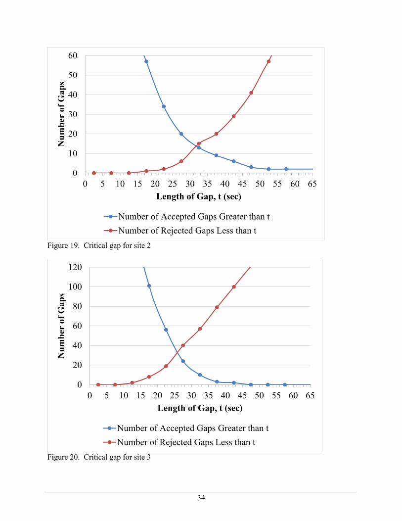
Figure 19. Critical gap for site 2 ...................................................................................................34
Figure 20. Critical gap for site 3 ...................................................................................................34
Figure 21. Example of narrow effective lane width from site 1 ...................................................36

xiii
Figure 22. Example of medium effective lane width from site 2 .................................................37
Figure 23. Example of wide effective lane width from site 3 .......................................................37
Figure 24. SR-20 work zone site ...................................................................................................64
Figure A-1: Example of Excel spreadsheet for video data from stationary cameras .....................71
Figure A-2: Example of Excel spreadsheet for video data from instrumented Honda Pilot .........72
Figure B-1. Small trucks. A) Panel truck. B) Garbage truck. C) Two-axle single-unit dump truck. D) Small delivery truck. E) Passenger cars with trailers .............................73
Figure B-2. Medium trucks. A) Three-axle single-unit dump truck. B) Concrete mixer. C) Passenger car with trailer using fifth wheel. D) Delivery truck. E) Single-unit cargo truck. ..................................................................................................................................75
Figure B-3. Large trucks. A) Tractor plus trailer. B) Tractor plus flatbed. C) Buses. ...............76
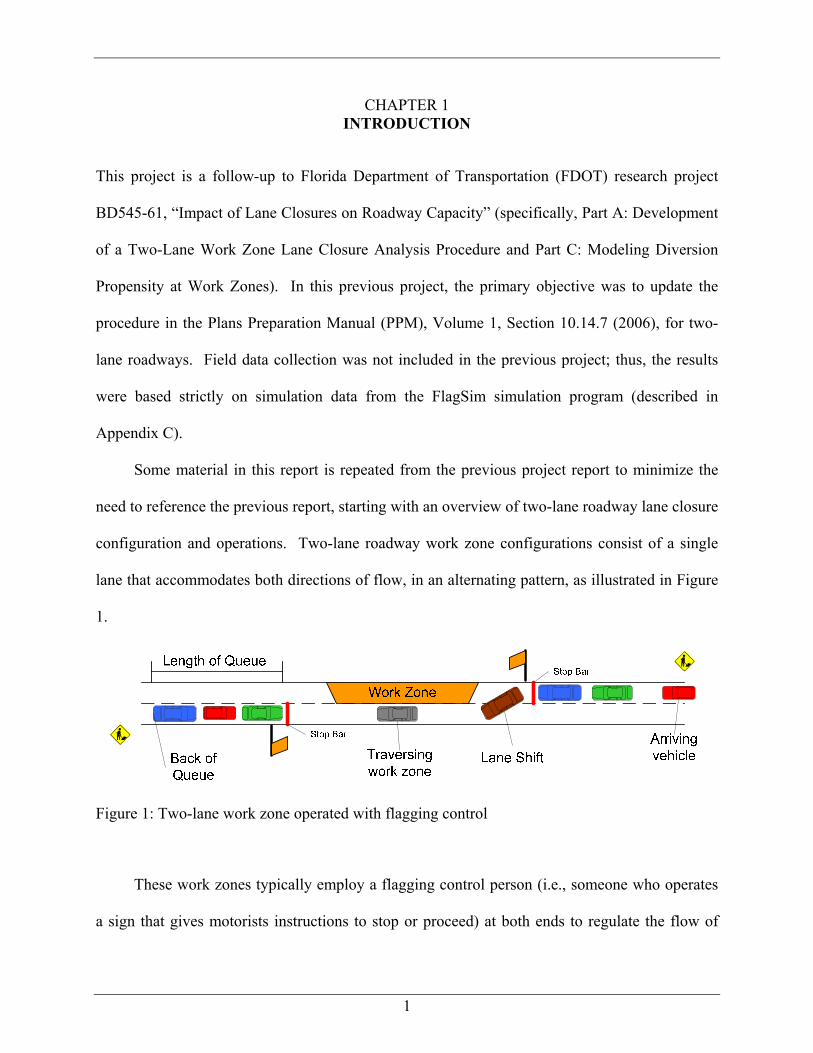
1
CHAPTER 1 INTRODUCTION
This project is a follow-up to Florida Department of Transportation (FDOT) research project
BD545-61, “Impact of Lane Closures on Roadway Capacity” (specifically, Part A: Development
of a Two-Lane Work Zone Lane Closure Analysis Procedure and Part C: Modeling Diversion
Propensity at Work Zones). In this previous project, the primary objective was to update the
procedure in the Plans Preparation Manual (PPM), Volume 1, Section 10.14.7 (2006), for two-
lane roadways. Field data collection was not included in the previous project; thus, the results
were based strictly on simulation data from the FlagSim simulation program (described in
Appendix C).
Some material in this report is repeated from the previous project report to minimize the
need to reference the previous report, starting with an overview of two-lane roadway lane closure
configuration and operations. Two-lane roadway work zone configurations consist of a single
lane that accommodates both directions of flow, in an alternating pattern, as illustrated in Figure
1.
Figure 1: Two-lane work zone operated with flagging control
These work zones typically employ a flagging control person (i.e., someone who operates
a sign that gives motorists instructions to stop or proceed) at both ends to regulate the flow of

2
traffic through the work zone. In some situations (usually where the lane closure is long or there
are a large number of driveways), a lead vehicle, called a pilot car, may be required to lead the
platoon of vehicles through the work zone.
Significant delay is incurred by motorists due to the lost time that accrues while the
opposing direction has the right-of-way. Additionally, both directions incur lost time when there
is a change in the right-of-way as the last vehicle that received the right-of-way must traverse the
entire length of the work zone; therefore, all vehicles must wait until the last vehicle has passed
the opposite stop location. The queue discharge process is similar to the operation of a
signalized intersection, but the queue discharge rate may be lower due to driver caution and
various work zone factors and activities.
Changing of the right-of-way is rarely performed in an optimal manner. Flag persons are
not trained on how to switch the right-of-way in such a manner as to minimize delay, or
otherwise optimize some particular performance measure (Evans, 2006). Generally, flag persons
change the flow direction due to queue and cycle length. The queue at the beginning of the
“green” period discharges at the saturation flow rate. After the initial queue dissipates, flag
persons usually extend the green to allow for vehicles still arriving. This extension time can be
lowered if there is a significant queue in the opposite direction. At this point, the flow through
the work zone will drop to the arrival rate. The arrival rate can be significantly lower than the
queue discharge rate on low volume roadways, thus increasing the overall average delay if
vehicles are queuing at the opposite approach (Cassidy and Son, 1994).
The typical performance measures for evaluating a work zone with flagging operations are:
Capacity – maximum vehicle throughput
Delay – time spent not moving, or at a slower speed than desired
Queue length – vehicle arrivals minus vehicle departures for a specified length of time

3
Problem Statement
Since there is not a single accepted national standard for analyzing work zone operations and
estimating performance measures, such as might be provided by the Highway Capacity Manual
(HCM) (TRB, 2010), transportation agencies are tasked with developing their own methods or
adopt/adapt ones from existing methods. Before the preceding research project, the FDOT
developed an analysis procedure for two-lane roadways with a lane closure that was a relatively
simple deterministic procedure, with rough approximations for work zone capacity and other
important parameter values. Through the previous project (BD545-61), a new analysis
procedure was developed that is sensitive to the major factors that influence work zone
performance measures. However, the main limitation from the BD545-61 project was the lack of
field data to use for calibrating the various simulation parameters. While some of these
parameters were set based on results of field data collection at signalized intersections from a
previous FDOT research project (BD545-51, Washburn and Cruz-Casas, 2007), it is likely that
there are still a number of significant differences in the queue accumulation and discharge
process at two-lane roadway lane closure sites. Furthermore, the extent to which conditions
within the work zone might further reduce drivers’ desired speed, relative to the posted speed,
was not known. Another aspect of the BD545-61 project was to develop a method to estimate
the amount of traffic diversion that occurs at a work zone location. The previous analysis
procedure in the PPM included the ‘Remaining Traffic Factor’ (RTF) term. This term accounts
for “The percentage of traffic that will not be diverted onto other facilities during a lane closure.”
(FDOT, 2006 PPM) The value to use for this input was left strictly to the analyst’s judgment, as
there was no method or quantitative guidance provided. Again, since field data were not
available in the BD545-61 project, a stated preference (SP) survey, via telephone, approach was
4
used to develop a method to estimate that amount of traffic diversion that will occur at a work
zone site.
Research Objective and Supporting Tasks
The primary objective of this project was to update the two-lane roadway with lane closure
analysis procedure developed under the previous project based on calibrating the FlagSim
simulation program to field data. An additional aspect of this that was not considered in the
BD545-61 project was to account for the effect of grade on the work zone performance
measures. An additional project objective was to update the RTF estimation method developed
under the BD545-61 project, as necessary, based on measured traffic demands (before and
during) at field sites. The tasks that were conducted to support completion of the objectives were
as follows:
Collected work zone operations data at three lane closure sites in north-central Florida.
Reduced and analyzed the field operations data.
Developed models for estimating work zone travel speed and saturation headway based on the field data.
Calibrated various FlagSim input parameters to yield a good match between simulated work zone traffic operations and field work zone operations.
Incorporated a new truck acceleration model into FlagSim (the same model used in FDOT Project BDK77-977-15) and updated truck characteristics in FlagSim based on analysis of weigh-in-motion (WIM) data from several two-lane highway sites.
Developed models for estimating work zone travel speed, saturation headway, queue delay, and queue length based on simulation data.
Revised the analysis procedure spreadsheet developed under the previous project to reflect the updated models developed in this project.
Collected local area traffic demand data at each field site, before and during the lane closure, (this was performed by FDOT staff) and analyzed the data.
Updated the RTF estimation model based on the field site local area traffic counts.

5
Document Organization
The remaining chapters in this report are organized as follows. Chapter 2 provides a brief
overview of the results of the preceding project as well as an overview of the original FDOT
PPM procedure (this material is repeated from the BD545-61 project report). Readers interested
in other research efforts and/or analysis tools applicable to two-lane roadways with a lane closure
should consult Chapter 2 of the BD545-61 project report. Chapter 3 describes the field site data
collection, analysis, and model development. Chapter 4 describes the simulation calibration
effort, the incorporation of the effect of grade, and the development of the final models to be
incorporated into the analysis spreadsheet tool. Chapter 5 provides a step-by-step overview of
the analysis procedure. Chapter 6 describes the results of the RTF task.

6
CHAPTER 2 REVIEW OF PREVIOUS FDOT ANALYSIS METHODS
This chapter presents a summary of the original FDOT PPM analysis procedure for two-lane
roadways with a lane closure and a summary of the results of the previous project (BD545-61).
Original FDOT PPM Analysis Procedure
The FDOT developed a lane closure analysis procedure for use with all road type classes.
The procedure is in the Plans Preparation Manual (PPM), Volume I, Section 10.14.7 (2006). The
procedure can analyze two-lane two-way work zones. In order to accommodate flagging
operations, the procedure attempts to determine the peak hour volume and the restricted capacity.
From these two values, the time during when lane closures can occur without creating excessive
delays is determined.
This procedure’s main limitation is that capacity is an input, and the given capacities were
not specific to two-lane work zones. With capacity not based on a flagging work zone value, the
procedure quite likely will be unable to model the field conditions accurately. Another limitation
with modeling flagging operations with this procedure is that it is based on only the ratio of
green time to the cycle length. This assumption does not take in to account the differences in
delays of flagging operations, such as the lost time due to the traversing the work zone, startup
lost time, and the variation of extended green time.
The capacity is adjusted by the work zone factor (WZF) shown in Table 1. The WZF is
used instead of a calculated travel time based on a typical speed. All of the lost time is also
incorporated in to the WZF. This is a simplistic adjustment to incorporate these important
factors. The travel time through the work zone is an easy calculation, which would make a
logical factor. One of the problems is the WZF is not adjusted by speed and is not documented
by what speed the factor is based on. This is an important question, as speeds through a work
7
zone can be quite different for an intense construction operation like chip and seal versus a less
intense operation such as shoulder work.
Table 1. FDOT PPM Analysis Method Work Zone Factor (WZF)
The FDOT PPM lane closure analysis procedure is as follows:
1. Select the appropriate capacity (c) from the table below:
LANE CLOSURE CAPACITY TABLE
Capacity (c) of an Existing 2-Lane-Converted to 2-Way, 1-Lane=1400 veh/h
Capacity (c) of an Existing 4-Lane-Converted to 1-Way, 1-Lane=1800 veh/h
Capacity (c) of an Existing 6-Lane-Converted to 1-Way, 1-Lane=3600 veh/h
Therefore, for a two-lane highway work zone, the capacity (c) is 1400 veh/h.
2. The restricted capacity (RC) is then calculated taking into consideration the following
factors:
TLW = Travel Lane Width
LC = Lateral Clearance. This is the distance from the edge of the travel lane to the obstruction (e.g., Jersey barrier)
WZF = Work Zone Factor. This factor is proportional to the length of the work zone. It is only used in the procedure for two-lane two-way work zones.
WZL (ft.) WZF WZL (ft.) WZF WZL (ft.) WZF200 0.98 2200 0.81 4200 0.64400 0.97 2400 0.8 4400 0.63600 0.95 2600 0.78 4600 0.61800 0.93 2800 0.76 4800 0.591000 0.92 3000 0.74 5000 0.571200 0.9 3200 0.73 5200 0.561400 0.88 3400 0.71 5400 0.541600 0.86 3600 0.69 5600 0.531800 0.85 3800 0.68 5800 0.512000 0.83 4000 0.66 6000 0.5

8
OF = Obstruction Factor. This factor reduces the capacity of the travel lane if the one of the following factors violates their constraints: TLW less than 12 ft and LC less than 6 ft.
G/C = Ratio of green time to cycle time. This factor is applied when the lane closure is through or within 600 ft of a signalized intersection.
ADT = Average Daily Trips. This value is used to calculate the design hourly volume.
The RC for roadways without signals is calculated as follows:
RC (Open Road) = c OF WZF [1]
If the work zone is through or within 600 feet of a signalized intersection, then RC is
determined by applying the following additional calculation.
RC (Signalized) = RC (Open Road) G/C [2]
If Peak Traffic Volume ≤ RC, there is no restriction on the lane closure. That is, if the
peak traffic volume is less than or equal to the restricted capacity, the work zone lane
closure can be implemented at any time during the day.
If Peak Traffic Volume > RC, calculate the hourly percentage of ADT at which a lane
closure will be permitted.
Open Road% = RTFPSCFDATC
OpenRoadRC
)(
[3]
where
ATC = Actual Traffic Counts. The hourly traffic volumes for the roadway during the desired time period.
D = Directional distribution of peak hour traffic on multilane roads. This factor does not apply to a two-lane roadway converted to two-way, one-lane.
PSCF = Peak Season Conversion Factor RTF = Remaining Traffic Factor. The percentage of traffic that will not be diverted onto
other facilities during a lane closure. Signalized% = (Open Road %) (G/C)
Plot the 24-hour traffic, relative to capacity, to determine when a lane closure is
permitted.

9
Revised Analysis Procedure through FDOT Project BD545-61
Overall Analysis Procedure
As described above, the original FDOT analysis procedure in the PPM is fairly simple and
considers a limited number of factors. Consequently, there is a very limited range of field
conditions for which this method will yield reasonably accurate results. Furthermore, the only
output from the method is work zone capacity. The objective of project BD545-61was to
develop an analysis procedure for two-lane roadway work zones (with a lane closure) that was
more robust, both in terms of inputs and outputs, than the FDOT’s current PPM method. The
FDOT also had the requirement that this new procedure still be easy to use.
A custom microscopic simulation program, FlagSim, was used to generate the data used in
the development of the models contained in the new analysis procedure. Specifically, models
were developed to estimate work zone travel speed, saturation headway, queue delay, and queue
length, as follows.
i
ii
HVLMin
PostedSpddWorkZoneSp
1063336.0)10560),5280((
000601.0706381.0608474.4 [4]
where
WorkZoneSpdi = estimated average travel speed of vehicles through the work zone for direction i (mi/h)
PostedSpdi = the posted speed, or maximum desirable travel speed of vehicles, through the work zone for direction i (mi/h)
L = work zone length (mi) HVi = percentage of heavy vehicles in the traffic stream for direction i
137.2
100145)45,(00516.0192.1_
iiisat
HVspeedMinh [5]
where
isath _ = saturation headway for direction i (s/veh)
speedi = average travel speed downstream of stop bar for direction i (veh/h)
10
HVi = percentage of heavy vehicles in the traffic stream for direction i
iii
iii
gHVg
CsvCgyTotalQDela
001376.0148503.0
003387.0(%)/242061.0(%)/276980.0 [6]
where
TotalQDelayi = total queue delay for a 1-hr time period for direction i (veh-hr) (gi /C) = average effective green time to average cycle length ratio for direction i (expressed as a percentage) (v/s)i = volume to saturation flow rate ratio for direction i (expressed as a percentage) C = average cycle length (sec)
ig = average green time for direction i (sec)
HVi = percentage of heavy vehicles in the traffic stream for direction i
iii
iii
gHVg
CsvCgngthMaxQueueLe
003199.0299197.0
0006855.0(%)/598965.0(%)/616983.0 [7]
where
MaxQueueLengthi = average maximum queue length per cycle for direction i (veh/cycle) Other terms are as previously defined.
The analysis procedure also employs calculation elements consistent with the analysis of
signalized intersections. This procedure is much more robust than the original PPM procedure,
and the results match well with the simulation data. The analysis procedure was implemented
into an easy-to-use spreadsheet format. Screen captures of the analysis spreadsheet are shown in
Figure 2 and Figure 3.

11
Figure 2. Analysis worksheet tool developed in FDOT project BD545-61 screen capture (1-hour analysis)
12
Figure 3. Analysis worksheet tool developed in FDOT project BD545-61 screen capture (24-hour analysis)
While it was felt that the results of this project (BD545-61) provided significant improvements
over the existing FDOT PPM procedure, there were several areas that were identified that could
benefit from additional research, as follows:
One obvious limitation to the results of this project is the lack of field data for verification/validation of several aspects of the simulation program. Although certain parameter values used in the simulation program were compared for consistency to field data values obtained from the Cassidy and Son research (1994), most of their field sites utilized a pilot car; thus, their parameter values may not be directly comparable to sites that do not use a pilot car. Field data should be collected at several sites, under only flagging control, to confirm the following factors:
o Saturation flow rates and/or capacities What are typical values, and how do they differ due to traffic stream
composition? Are they different by direction, e.g., due to the required lane shift in
one direction? o Travel speeds through the work zone
Are they related to, or independent of, posted speed limits? Are they different by direction due to the lane crossover at the
beginning of the work zone? Son (1994) states from their literature review that vehicles in the blocked travel direction usually have lower speeds than the opposite direction.
o Startup lost time What are typical values?
13
Are they different by direction? o Flagging methods
Is a gap-out strategy ever applied, and if so, how? Is a maximum green time used, and if so, what value? Is a green time extension used, and if so, what value?
Remaining Traffic Factor (RTF) Task
When estimating the hourly traffic demand, the FDOT PPM procedure applies a
"Remaining Traffic Factor" (RTF) to the observed hourly traffic demand without the lane
closure. The RTF accounts for possible traffic diversion during the lane closure. However, no
guidance has been offered on how to obtain the value of the RTF in the PPM.
The purposes of this research task were twofold. First, diversion behaviors at work zones
were modeled in a discrete choice modeling framework. A stated preference survey was carried
out to obtain the data on drivers’ diversion propensity from work zones. By calibrating a Logit
model with the data, we identified three major factors that influence drivers’ diversion decisions,
namely, travel time, work zone location, and weather condition. For other factors, such as trip
purpose and drivers’ social economic characteristics, we found no evidence that they are
important in drivers’ decision making about diversion at work zones. The calibrated model
provides us with more insight on drivers’ work zone diversion behaviors and may be used to
forecast diversion rates or be incorporated into a work zone traffic analysis tool.
Second, we proposed two procedures, namely open-loop and closed-loop, to apply the
calibrated binary Logit model to estimate the RTF. The former directly applies the choice model
without considering the feedback of remaining and diverted flows on travel times. It may be
more appropriate to be used for a short-term work zone lane closure. The latter applies the
notion of equilibrium to maintain the consistency between travel times and flows at different
routes. Therefore, it may better replicate the situation at a long-term work zone. Based on the
14
combinations of the weather condition and work zone location, four Fisk’s stochastic user
equilibrium models have been formulated, which can be solved by the Excel solver to compute
the RTF. An Excel tool was developed to facilitate the computation, screen captures of which
are shown below in Figure 4 and Figure 5.
Figure 4. RTF estimation spreadsheet tool developed in FDOT project BD545-61 screen capture
(1)
Figure 5. RTF estimation spreadsheet tool developed in FDOT project BD545-61 screen capture
(2)

15
CHAPTER 3 FIELD DATA COLLECTION AND ANALYSIS
This chapter describes the data requirements for calibration of the FlagSim simulation program.
This is followed by discussion on the sites where data were collected, the data collection
procedure undertaken, and a brief description of the data collected at these sites. The data
processing procedure is then described, and results from this processing are presented and
discussed. Lastly, the work zone speed and saturation headway models developed from the field
data are presented.
Data Requirements
In order to calibrate the FlagSim simulation program to field conditions, it was first necessary to
identify what type of data were necessary to perform this task. Based on the simulation program
internal models and possible outputs from this program, the following data parameters were
identified:
Length of lane closure
Posted speed in work zone
Posted speed of work zone approach
Travel time of each vehicle through work zone for each phase
Vehicle type of each vehicle entering the work zone per phase
Number of vehicles entering the work zone per phase
Average speed of vehicles in the work zone per phase
“Green” time per phase
Startup lost time per phase
Queue delay per phase
Queue length per phase
16
Saturation headway per phase
Type of flagging control used at the lane closure
These parameters collectively comprise the inputs and outputs of the FlagSim program. In
addition, it was also necessary to obtain some data regarding traffic operations within the lane
closure. Specifically, how traffic operations were impacted by construction taking place in the
work zone.
Description of Study Sites
To facilitate the calibration of the FlagSim program, it was necessary to identify several study
sites that provided different traffic characteristics and work zone conditions. Ultimately, field
data were collected from three sites. Two of these sites were in fairly rural locations, which
featured longer lane closure lengths and lower demand volumes. The third site was less rural in
nature and featured shorter lane closures and higher demand volumes. The general location of
these sites is indicated in Figure 6. Each of these sites is discussed in more detail in the
following sections.
Figure 6. Work zone site locations

17
Site 1 Description
The first field site identified was located on SR-145 between the cities of Madison, FL and
the Florida/Georgia border. This road is a frequent logging route and features a large percentage
of heavy vehicles. It is more rural in nature, and the total AADT on this road was approximately
2000 in 2010. The length of lane closures on this roadway varied between 1.29 and 1.95 miles.
The distance weighted average of the posted speed in these lane closures was mainly 55 mi/h,
while one lane closure had an average posted speed of 60 mi/h. Construction activities consisted
mainly of milling and resurfacing. Figure 7 shows a general map of the location of the
construction along this road. It should also be noted that a few access roads are located along
this stretch of road and had some contribution to the traffic through the lane closures. These
roads primarily provide access to residential neighborhoods.
Figure 7. Extent of construction along SR-145 (site 1)

18
Site 2 Description
The second field site identified was located on SR-235 between the cities of Alachua, FL
and La Crosse, FL. This road is more rural in nature, and the total AADT on this road was
approximately 2800 in 2010. The length of lane closures on this roadway varied between 1.63
and 2.00 miles. The distance weighted average of the posted speed in these lane closures was 55
mi/h. Construction activities consisted mainly of milling and resurfacing. Occasional access
roads are located along this stretch of road. These roads primarily provide access to more rural
residences although a couple provided access to religious institutions. Figure 8 shows a map of
where construction was being performed along this stretch of road.
Figure 8. Extent of construction along SR-235 (site 2)
19
Site 3 Description
The third field site identified was located on SR-20 between the city of Hawthorne, FL and
the intersection of SR-20 and SR-21. This road is heavily trafficked by commuters in the both
the morning and afternoon. As a result, this road is less rural in nature during these peak periods
and features larger volumes of traffic compared to sites 1 and 2. The total AADT on this road
was approximately 8200 in 2010. The length of lane closures on this roadway varied between
0.74 and 1.63 miles with only one lane closure being over 1 mile. The distance weighted
average of the posted speed in these lane closures was mainly 55 mi/h, while one lane closure
had an average posted speed of 50 mi/h. Construction activities performed at this site primarily
consisted of shoulder reconstruction and sodding. Figure 9 shows a map of the location of the
construction along this road. Occasional access roads are located along this stretch of road.
These roads can serve as alternate routes to the nearby city of Hawthorne and SR-21.
Figure 9. Extent of construction along SR-20 (site 3)

20
Data Collection Procedure
To obtain adequate data for calibration of the FlagSim simulation program, it was desirable to
obtain approximately 4 hours of data each day for 4 different days at each of the three study
sites. Due to the microscopic nature of the data required for this study, video was selected as the
method by which to collect the data. For each study site, stationary cameras were placed at each
end of the lane closures to observe vehicles entering and exiting the work zone, queuing at the
work zone, and flagging operations. The video feed was recorded to an external hard drive
recorder which was secured in a Pelican case next to the camera. Both the camera and hard drive
recorder were powered by a single 12-volt battery. An example of the type of equipment and set
up used to collect the data is shown in Figure 10.
Figure 10. Video camera and external hard drive recorder setup used for data collection
21
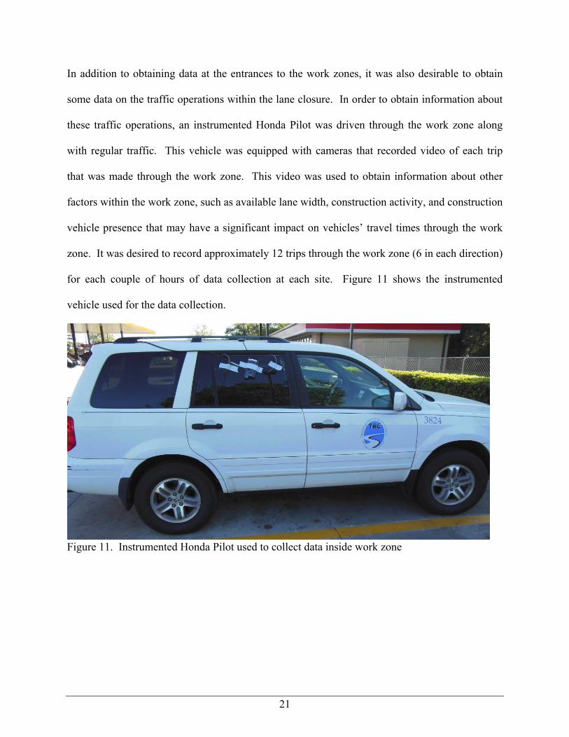
In addition to obtaining data at the entrances to the work zones, it was also desirable to obtain
some data on the traffic operations within the lane closure. In order to obtain information about
these traffic operations, an instrumented Honda Pilot was driven through the work zone along
with regular traffic. This vehicle was equipped with cameras that recorded video of each trip
that was made through the work zone. This video was used to obtain information about other
factors within the work zone, such as available lane width, construction activity, and construction
vehicle presence that may have a significant impact on vehicles’ travel times through the work
zone. It was desired to record approximately 12 trips through the work zone (6 in each direction)
for each couple of hours of data collection at each site. Figure 11 shows the instrumented
vehicle used for the data collection.
Figure 11. Instrumented Honda Pilot used to collect data inside work zone

22
Description of Data Obtained from Study Sites
Video from Stationary Cameras
A total of 34.5 hours of data was obtained from the three study sites. Data for site 1 were
collected on 10/25/2011, 10/27/2011, and 10/28/2011. Approximately 4 hours of data was
collected on 10/25/2011 and 10/27/2011, while 3 hours of data were collected on 10/28/2011.
Figure 12 shows a frame capture from one of the videos recorded at this site.
Figure 12. Entrance to work zone at site 1 on 10/25/2011
Data for site 2 were collected on 02/01/2012, 02/03/2012, 02/06/2012, 02/08/2012, and
02/09/2012. Unfortunately, the data collected on 02/01/2012 did not prove useful as it contained
very minimal amounts of traffic (only 1 to 3 vehicles in queue). This very low traffic demand
does not lend itself well to reliable calibration of the FlagSim program. As a result, these data

23
was not used for the purposes of this project. Approximately 13.5 hours of data were collected
on the remaining three days at the site. Specifically, 6, 2.5, 1.5, and 3.5 hours of data were
collected on 02/03/2012, 02/06/2012, 02/08/2012, and 02/09/2012, respectively. Figure 13
shows a frame capture from one of the videos recorded at this site.
Figure 13. Entrance to work zone at site 2 on 2/3/2012
Data were collected from site 3 on 01/21/2013, 01/23/2013, 01/24/2013, and 01/25/2013.
Because this site featured shorter lane closures, it was necessary for the construction crew to
move the location of the lane closure more frequently as the construction progressed throughout
the day. As a result, the length and location of the lane closure varied throughout each day.
Approximately 10 hours of data were collected at this site. Specifically, 2, 2.5, 3, and 2.5 hours

24
of data were collected on 01/21/2013, 01/23/2013, 01/24/2013, and 01/25/2013, respectively.
Figure 14 shows a frame capture from one of the videos recorded at this site.
Figure 14. Entrance to work zone at site 3 on 1/25/2013
Video from Instrumented Honda Pilot
A total of 117 trips were made through the various work zones at the three sites. Fifty-one
trips were made at site 1, 29 trips were made at site 2, and 37 trips were made at site 3. Figure
15, Figure 16, and Figure 17 show frame captures from the in-vehicle videos recorded at sites 1,
2, and 3, respectively.

25
Figure 15. Video from instrumented Honda Pilot at site 1 on 10/25/2011
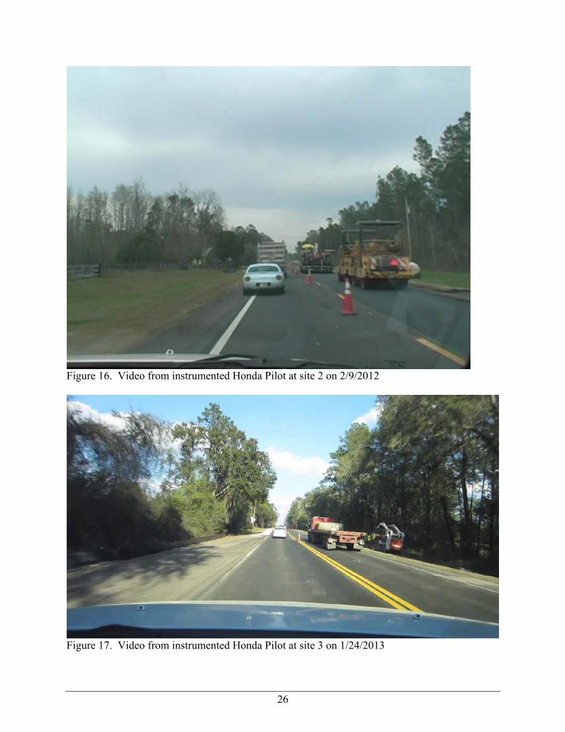
26
Figure 16. Video from instrumented Honda Pilot at site 2 on 2/9/2012
Figure 17. Video from instrumented Honda Pilot at site 3 on 1/24/2013
27
Data Processing
Once the data had been collected at a lane closure site, it was necessary to process these data to
obtain the information needed for the calibration of FlagSim. This processing required watching
the videos from both the stationary cameras as well as from the instrumented Honda Pilot.
Pertinent information from these videos was recorded into Excel spreadsheets. The data items
that were obtained from these two video sources are discussed in the following sections.
Before proceeding with the discussion, the following definitions are provided for several
terms used throughout the remainder of this report:
Green time: “Green” time, which means “go time”, is the time during which, for a given travel direction, the flag person’s paddle/sign is displaying ‘slow’. The total green time is calculated as the difference in time from when the flag person changes the paddle/sign from ‘stop’ to ‘slow’ and back to ‘stop’. The definition of this term as used in this study is consistent with the definition of ‘displayed green time’ in signalized intersection analysis.
Red time: “Red” time, which means “stopped time”, is the time during which, for a given travel direction, the flag person’s paddle/sign is displaying ‘stop’. The total red time is calculated as the difference in time from when the flag person changes the paddle/sign from ‘slow’ to ‘stop’ and back to ‘slow’. The definition of this term as used in this study is consistent with the definition of ‘displayed red time’ in signalized intersection analysis.
Phase time: The phase time was calculated as the green time plus the time it takes the last vehicle to enter the work zone during the displayed green to exit the work zone. More generally, this is referred to as green time plus work zone travel time. There were some cases where the flag person allowed one or more vehicles to enter the work zone after he/she turned the paddle/sign to ‘stop’. In these cases, the time that the flag person changed the flag to ‘stop’ was changed to the time that the last vehicle entered the work zone. However, this was not done in cases where the vehicle(s) that entered after the paddle/sign had been changed to ‘stop’ were associated with the construction activities (i.e., the vehicle did not exit the work zone during that phase).
Lost time: As used in this study, the definition of total lost time for a phase is consistent with the definition as used in signalized intersection analysis—that is, the time during which vehicles for a given approach/direction are not moving. This lost time is typically separated into a ‘startup’ lost time component and a ‘clearance’ lost time component. The startup lost time is considered to be the difference between the time when the front bumper of the last vehicle to exit the work zone crosses the stop bar and the time when the front bumper of the first vehicle of the opposing direction enters the work zone. The
28
clearance lost time is considered to be the travel time through the lane closure area of the last vehicle for the opposing direction to enter the work zone, for a given phase.
Cycle time: The cycle time (or length) is calculated as the difference in time from when the flag person for a given travel direction changes the paddle/sign from ‘stop’ to ‘slow’ to ‘stop’ and back to ‘slow’ again. This is equivalent to the phase time for one travel direction plus the phase time for the opposing travel direction.
Data from Stationary Camera Video
Some of the parameters outlined in the data requirements section were obtained from the
stationary camera videos. An Excel spreadsheet was used to organize data for each travel
direction for each day and site. An example of the type of Excel spreadsheet created for the
stationary camera video data is shown in Appendix A. The data are organized for each phase
observed from the video recordings. For each phase, certain information was recorded in order
to obtain data for the parameters outlined in the data requirements section. This section
discusses how such information was used to determine values for the parameters in the data
requirements section. A discussion on what type of flagging control was employed in the field is
also discussed.
Displayed paddle/sign indication change times
The time at which a flag person for a given travel direction change the displayed indication
(‘slow’ or ‘stop’) was recorded. This allowed several of the above-defined time-related
definitions to be calculated.
Vehicle type and work zone travel time
A record of each vehicle that entered the work zone was created. Each record contained
the vehicle’s work zone entry time and work zone exit time (for those vehicles that exited the
work zone). Using the work zone entry and exit times of the vehicle, the work zone travel time
for the vehicle was obtained. The vehicle was also classified as either a passenger car (PC),

29
small truck (ST), medium truck (MT), or large truck (LT). Pictures showing how the truck
categories were classified can be found in Appendix B.
Average speed of vehicles in the work zone per phase
The work zone travel times for all vehicles entering the work zone during a given phase
were averaged. This average work zone travel time was then used along with the length of the
lane closure to determine the average speed of vehicles through the work zone for the phase.
Number of vehicles entering the work zone per phase
The time when each flag person switched their paddle/sign was recorded. From this
information and the work zone entry time for each vehicle, the number of vehicles entering the
work zone for each phase could be determined. It was also possible to determine how many
vehicles of each different vehicle classification (e.g., passenger car, small truck) entered the
work zone during each phase.
Startup lost time
The amount of startup lost time is a function of several factors. The first delay occurs as
the last vehicle exiting the work zone travels from the work zone exit point to a safe distance in
order to allow the next direction of vehicles to proceed. The exiting vehicle must maneuver the
lane switch area and pass the first few vehicles queued. Second, additional time is needed for the
flag person to switch their paddle/sign, such as the time it takes the flag person to determine
when the work zone is clear. Finally, there is lost time for the first vehicle reacting to the change
of the sign, similar to vehicles’ startup lost time at a signalized intersection.
The startup lost time for each phase was calculated by taking the difference between the
time the first vehicle in queue entered the work zone and the time the last vehicle traveling in the
opposing direction exited the work zone. If the last vehicle traveling in the opposing direction
exited after the flag person changed the paddle/sign to ‘slow’, the startup lost time calculation

30
was modified. In this case, the startup lost time was calculated by taking the difference between
the time the first vehicle in queue entered the work zone and the time the flag person changed the
paddle/sign to ‘slow’.
The mean and standard deviation of the startup lost time was determined for each site.
These values are shown in Table 2. From this table, it can be seen that the first two sites had
larger means and standard deviations than the third site. This is likely a result of the longer lane
closures at these sites. Since these sites were more rural in nature and had longer lane closures,
the amount of time that some drivers were waiting to enter the work zone was in the order of 4 to
7 minutes. As a result, some drivers were not paying as much attention to the flag person and
took a little more time to start up after the flag person changed the paddle/sign to ‘slow.’ This
resulted in larger startup lost time values compared to those obtained from the third site, which
had shorter lane closures and was less rural in nature.
Table 2. Startup Lost Time Values Determined for Each Site
Site #
Startup Lost Time
Mean (s) Std. Dev. (s)
1 14.73 10.56
2 15.18 11.56
3 10.00 4.75
Queue length
The queue length for each phase and direction was obtained by simply counting the
number of vehicles in queue prior to the flag person changing the paddle/sign to ‘slow’.
Saturation headway
The saturation headway for each phase and direction was obtained by using the work zone
entry times of the first eight vehicles in queue. Specifically, this value was calculated by taking

31
the difference between the work zone entry times of the first and eighth vehicle in queue and
dividing by the number of headways between the first and eighth vehicle.
Type of flagging control employed
After watching the videos from the stationary cameras, it seemed as though most flag
persons were using a ‘distance gap out’ mechanism to judge when to switch the travel direction
right-of-way. The main input for this type of flagging control in FlagSim is the mean distance
gap out value. From watching the videos, it was difficult to determine the distance gaps that the
flag persons were using to control their paddle/sign. Therefore, the mean distance gap out value
could not be determined with much accuracy. The time gaps associated with the distance gaps
that the flag persons used, however, could be easily determined from the videos. While it is
unrealistic for a flag person to directly employ a ‘time gap out’ method in the field, since the flag
person would have to constantly look at a timing device, the use of a time gap out flagging
control would allow for the best calibration of the FlagSim program. Therefore, a time gap out
flagging control was used in place of a distance gap out flagging control for calibration of the
FlagSim program.
In order to use this time gap out flagging control for the FlagSim calibration, it was
necessary to determine the mean and standard deviation of the time gap out values used by the
flag persons. The mean time gap out value was determined using a critical gap procedure.
Specifically, Raff’s critical gap method (1950) was used, which required the use of the gaps the
flag persons accepted as well as rejected. This is the same method used to identify critical gap
acceptance values for the unsignalized intersection analysis procedure in the HCM.
An accepted gap was calculated by taking the difference between the work zone entry
times of two consecutive vehicles that entered the work zone during the same phase. Each phase
contained multiple accepted gaps if more than two vehicles entered the work zone during the

32
phase. A rejected gap was calculated for a given phase by taking the difference between the time
the first vehicle arrived at the work zone after the flag person changed the paddle/sign to ‘slow’
and the time the last vehicle in the phase entered the work zone. There was only one rejected
gap per phase.
Rather than estimating the time gap out values to the nearest second, it was determined that
it would be more beneficial to estimate the time gap out values to the nearest 5 seconds. This
was because the actual values of the accepted and rejected gap values were only accurate within
a couple of seconds, since the work zone entry times could only be obtained from the videos to
the nearest second. Therefore, the accepted and rejected gap values were placed into 5 second
bins between 0 and 60 seconds. Values greater than or equal to 60 seconds were placed into a
separate bin, since a very small number of gaps greater than or equal to 60 seconds were
accepted by the flag persons.
After the accepted and rejected gaps were placed into these bins, the critical time gap out
value was determined. A graph was created to show the cumulative number of accepted gaps
and rejected gaps for the different bins. From this graph the critical time gap out value was
determined by looking at the point where these cumulative curves intersected. This value was
used as the mean time gap out value in FlagSim. Since the critical time gap out value was only
accurate within 5 seconds, it was decided that a standard deviation of 5 seconds was appropriate
for the time gap out value.
Critical time gap out values were determined for each site. These values are shown in
Table 3. From this table, it can be seen that the first two sites had a larger mean critical time gap
out value as compared to the third site. This is likely a result of the longer lane closures and
smaller traffic demands at sites 1 and 2. Because the lane closures were longer and not as many

33
vehicles needed to enter the work zone, the flag persons would generally allow any late arriving
vehicles to enter the work zone, even if the vehicles were a good distance away from the work
zone. This in turn increased some of the accepted gap values, which resulted in a larger critical
gap. The graphs that were used to obtain the critical gap values for each site are shown in Figure
18, Figure 19, and Figure 20. The data used to create these plots can be found in Appendix A.
Table 3. Critical Time Gap Out Values Determined for Each Site
Site #
Critical Time Gap Out
Mean (s) Std. Dev. (s)
1 30 5
2 30 5
3 25 5
Figure 18. Critical gap for site 1
0
10
20
30
40
50
60
0 5 10 15 20 25 30 35 40 45 50 55 60 65
Nu
mb
er o
f G
aps
Length of Gap, t (sec)
Number of Accepted Gaps Greater than t
Number of Rejected Gaps Less than t
34
Figure 19. Critical gap for site 2
Figure 20. Critical gap for site 3
0
10
20
30
40
50
60
0 5 10 15 20 25 30 35 40 45 50 55 60 65
Nu
mb
er o
f G
aps
Length of Gap, t (sec)
Number of Accepted Gaps Greater than t
Number of Rejected Gaps Less than t
0
20
40
60
80
100
120
0 5 10 15 20 25 30 35 40 45 50 55 60 65
Nu
mb
er o
f G
aps
Length of Gap, t (sec)
Number of Accepted Gaps Greater than t
Number of Rejected Gaps Less than t

35
Video from Instrumented Vehicle
Video of trips made through the work zone in the instrumented Honda Pilot were used to
ascertain information about different factors within the work zone that may have an impact on
traffic operations in the work zone. Specifically, it was desirable to determine what factors may
have an impact on vehicles’ speeds through the work zone. From watching the videos, it was
observed that the following factors may have influenced vehicles’ speeds:
Effective lane width – the width of the pavement available for vehicles to drive on (includes paved shoulders)
Construction activity – level of construction activity taking place (e.g., milling and resurfacing, shoulder work, sodding)
Construction vehicle presence – number of stationary construction vehicles parked on the closed lane in close proximity to vehicles traveling on the open lane
Travel direction of closed lane – whether drivers will have to travel in the “opposing” lane through the work zone
Percentage of construction vehicles entering the work zone – the percent of construction vehicles that entered the work zone during a phase but did not exit
Information about the first four factors above was determined from the instrumented
Honda Pilot video. Information about the last factor, percentage of construction vehicles
entering the work zone, was determined from both the stationary camera video and instrumented
Honda Pilot video. An Excel spreadsheet was used to organize information about each of these
factors for all recorded trips through the work zone. A screenshot of this spreadsheet can be
found in Appendix A. The type of information obtained for each of these factors is discussed
below in its respective section.
Effective lane width
Based on observations from the videos, it was hypothesized that as the lane width available
to drivers in the work zone decreased, the average speed of vehicles in the work zone also
decreased. Therefore, this effective lane width was recorded for each trip made through the
work zone by the instrumented Honda Pilot. It was difficult to determine a precise numeric

36
value for the effective lane width from the videos, so this variable was categorized into three
general levels (narrow, medium, and wide).
Narrow lane widths were assigned for lanes that had no, or a very narrow, shoulder and
cones placed inside the lane. Figure 21 shows an example of a narrow effective lane width.
Medium lane widths were assigned for lanes that had a small shoulder and cones placed outside
the lane or on the centerline. Medium lane widths were also assigned for lanes that had a
relatively wide shoulder and cones placed inside the lane. Figure 22 shows an example of a
medium effective lane width. Wide lane widths were classified for a lane with a relatively wide
shoulder and cones placed outside the lane or on the centerline. Wide lane widths were also
assigned for lanes that had a narrow shoulder but cones placed outside the lane. Figure 23 shows
an example of a wide effective lane width.
Figure 21. Example of narrow effective lane width from site 1

37
Figure 22. Example of medium effective lane width from site 2
Figure 23. Example of wide effective lane width from site 3

38
Construction activity
The construction activity in the work zone also appeared to have an effect on vehicles’
speeds in the work zone. Therefore, the construction activity was recorded for each trip through
the work zone. Since a numeric value was not able to be put on the construction activity, three
different categorical levels were used for this variable (low, medium, and high). Low
construction activity was considered for activities such as sodding, shoulder work, or any other
activity that required few construction vehicles or equipment to operate close to the open travel
lane. Medium construction activity was considered for activities such as milling or resurfacing
or any other activity that required several construction vehicles or pieces of equipment to operate
close to the open travel lane. High construction activity considered for activities such as both
milling and resurfacing taking place at the same time or any other activity that required a large
number of construction vehicles or equipment to operate close to the open travel lane.
Construction vehicle presence
The number of stationary construction vehicles that were in proximity to the open travel
lane was also thought to have some effect on vehicles’ speeds in the work zone. Since some
construction vehicles (e.g., dump trucks, rolling equipment) would sit on the closed travel lane in
close proximity to the open travel lane, it was thought that drivers may tend to slow down when
driving past these vehicles. This could lead to lower average speeds in the work zone. The
presence of construction vehicles was recorded for each trip made with the instrumented Honda
Pilot. Developing a precise numeric value for this factor was not practical; thus, three different
categorical levels were used (low, medium, and high). Low construction vehicle presence was
defined as having very few construction vehicles in the work zone, and if there were vehicles,
they were not close to the open travel lane. Medium construction vehicle presence was defined
as having a few construction vehicles in the work zone. These were mainly pickup trucks or

39
other smaller pieces of construction equipment, but there could be a few larger construction
vehicles (e.g., dump trucks). A few of these construction vehicles would be close to the open
travel lane, but the majority would not. High construction vehicle presence was defined as
having a large number of construction vehicles in the work zone. These vehicles would consist
of larger construction vehicles (e.g., dump trucks, semi-tractor trailers), and many of these
vehicles would be in close proximity to the open travel lane.
Travel direction of closed lane
If a driver is traveling on the lane that is closed, he/she will have to temporarily switch
lanes and travel on the opposing lane when proceeding through the work zone. Since drivers are
not accustomed to driving in the opposite lane, they may be more cautious when proceeding
through the work zone. As a result, the average speed of vehicles in the work zone may be
slightly lower for the travel direction with the closed lane as opposed to the direction with the
open lane. The travel direction of the closed lane was recorded for each of the trips through the
work zone in the Honda Pilot.
Percentage of construction vehicles entering the work zone
When watching some of the videos, vehicles associated with the construction activities
(e.g., dump trucks) were seen departing from the open travel lane and moving onto the closed
travel lane to help with the construction activities. Before these vehicles moved off the open
travel lane and onto the closed travel lane, they usually decelerated, sometimes causing the
vehicles traveling behind them to slow down. As a result, the travel times of these vehicles may
have been extended due to this impedance by the construction vehicles. Information about how
many of these construction vehicles entered the work zone was not able to be accurately
determined from the instrumented Honda Pilot videos. Fortunately, this information could be
obtained from the stationary camera video. Therefore, the construction vehicles which entered
40
the work zone but did not exit were identified for each phase. These vehicles were temporarily
assigned a classification of CV, for construction vehicle, within the spreadsheet data logs. The
percentage of construction vehicles that entered the work zone was then determined for each of
the trips the Honda Pilot made through the work zone. It should be noted that most of the
construction vehicles that entered the work zone and did not exit were dump trucks.
Models from Field Data
Two models were estimated from the field data—one for average travel speed through the work
zone and one for the average saturation headway of vehicles discharging from a queue into the
work zone.
Work Zone Speed Model
With the impact to the overall cycle length due to the lost time caused by traversing the
work zone, the estimation of the work zone travel speed must be as accurate as possible. A
regression analysis was performed on all of the data recorded from the Honda Pilot trips through
the work zone (92 trips). The resulting model formulation is shown in Eq. 8.
MediumLWHVNarrowLWHVMedHighConstAct
NumVehlosedLaneTravelDirCPostedSpd
MediumLWNarrowLWHVdWorkZoneSp
ii
i
ii
_%2993.0_%5310.0_5092.2
0590.033.18501.0
_2328.8_9068.12%4694.04611.0
[8]
where
WorkZoneSpdi = average travel speed of vehicles through the work zone for phase i (mi/h) %HVi = percentage of heavy vehicles in the traffic stream for phase i LW_Narrow = 1 if the effective lane width is narrow, 0 otherwise LW_Medium = 1 if the effective lane width is medium, 0 otherwise PostedSpd = the posted speed limit through the work zone (mi/h) TravelDirClosedLane = 1 if vehicles are traveling in the direction of the closed lane (i.e.,
they perform a lane shift when entering and exiting work zone), 0 otherwise NumVehi = the number of vehicles entering the work zone for phase i ConstAct_MedHigh = 1 if the level of construction activity in the work zone is medium or
high, 0 otherwise
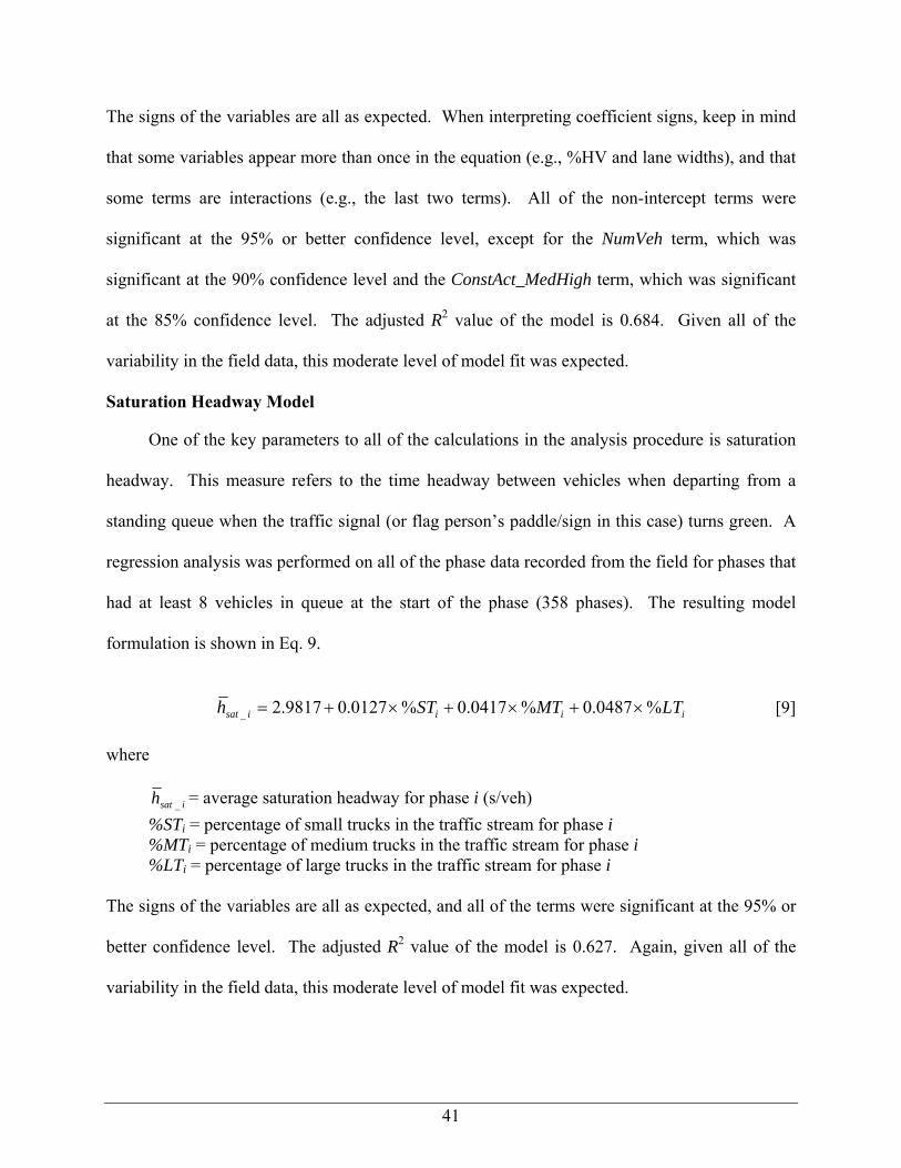
41
The signs of the variables are all as expected. When interpreting coefficient signs, keep in mind
that some variables appear more than once in the equation (e.g., %HV and lane widths), and that
some terms are interactions (e.g., the last two terms). All of the non-intercept terms were
significant at the 95% or better confidence level, except for the NumVeh term, which was
significant at the 90% confidence level and the ConstAct_MedHigh term, which was significant
at the 85% confidence level. The adjusted R2 value of the model is 0.684. Given all of the
variability in the field data, this moderate level of model fit was expected.
Saturation Headway Model
One of the key parameters to all of the calculations in the analysis procedure is saturation
headway. This measure refers to the time headway between vehicles when departing from a
standing queue when the traffic signal (or flag person’s paddle/sign in this case) turns green. A
regression analysis was performed on all of the phase data recorded from the field for phases that
had at least 8 vehicles in queue at the start of the phase (358 phases). The resulting model
formulation is shown in Eq. 9.
iiiisat LTMTSTh %0487.0%0417.0%0127.09817.2_ [9]
where
isath _ = average saturation headway for phase i (s/veh)
%STi = percentage of small trucks in the traffic stream for phase i %MTi = percentage of medium trucks in the traffic stream for phase i %LTi = percentage of large trucks in the traffic stream for phase i
The signs of the variables are all as expected, and all of the terms were significant at the 95% or
better confidence level. The adjusted R2 value of the model is 0.627. Again, given all of the
variability in the field data, this moderate level of model fit was expected.

42
CHAPTER 4 SIMULATION ANALYSIS AND RESULTS
This chapter describes the simulation aspect of this project. Because a wide range of input
conditions were not obtained from the field sites described in the previous chapter, it was
necessary to use simulation to be able to analyze the performance of two-lane roadways with a
lane closure across a wide range of conditions (e.g., length of lane closure, traffic demand, work
zone posted speed, etc.). The main purpose of the field data was to identify the appropriate
values for the various settings that affect the behavior of the vehicles and flagging operations in
the simulation program.
Two-lane work zones are unique in their operation. In order to model the operations
reasonably accurately, a simulation program must have the following capabilities at a minimum:
model the flagging control method used in the field
model vehicle arrivals at the work zone
model vehicles discharging from the stop line
model heavy vehicles, in addition to passenger cars
model vehicles traveling through the work zone
record various simulation results in order to allow for the following performance measures to be calculated, such as
o queue delay
o travel time delay due to reduced speeds
o queue length
o capacity
Most, if not all, existing commercially available simulation packages do not explicitly
provide for modeling work zones on two-lane roadways, nor are they easily configured for such
43
modeling, particularly because of the unique aspects of flagging control. The FlagSim
simulation program was used for the simulation aspects of this project. This program was also
used for the predecessor project to this one; however, it has undergone a number of
enhancements since that time. A detailed overview of the program is provided in the Users
Guide, which is included in Appendix C of this report.
Calibration
The calibration effort consisted of initially setting the various driver and vehicle
parameters in FlagSim to values consistent with observations from the field data and/or other
data sources. A large number of simulation runs, with a range of input conditions consistent with
the range of input conditions observed in the field, were then made. The simulation results for
average work zone travel speed and average saturation headway were then compared to the field
values. This process was repeated many times, with small revisions made to one or more of the
driver parameters each time. The driver parameter values that resulted in the best fit of the
simulation data to the field data were retained for further use in the FlagSim simulation runs.
The vehicle parameters were not varied from their initial settings. The vehicle and driver
parameters are accessed through the ‘Advanced Vehicle/Driver Parameters’ screen in FlagSim
(see Users Guide in Appendix C). These parameters and their settings are described in the
remainder of this section.
Vehicle Parameters
Vehicle Dimensions (length, width, height)
The three truck classifications discussed in the previous chapter were generally matched to
the standard FHWA classifications as follows:
Small Truck—Class 5 and 6 Medium Truck—Class 8 Large Truck—Class 9, 11, and 12
44
The dimensions of the three truck types were set accordingly. The passenger car dimensions
were based on common sedan-type vehicle—specifically a Honda Civic. The selected
dimensions are shown in Table 4.
Maximum Acceleration
Maximum acceleration is not an input to FlagSim. FlagSim now uses a full vehicle
dynamics modeling approach to determine the maximum acceleration of a vehicle. This model
takes into account the vehicle’s physical (such as frontal area, drag coefficient, and weight) and
drivetrain (such as engine output and transmission gearing) characteristics to determine the
tractive effort available to accelerate the vehicle at every time step during the simulation. This
approach also allows roadway grade to be accounted for, as this affects the grade resistance in
the acceleration calculations. This approach for modeling maximum acceleration is described in
more detail in the FlagSim Users Guide (see Appendix C).
Vehicle Weight
For another FDOT research project (BDK77-977-15), weigh-in-motion (WIM) data were
obtained for numerous locations across the state for a recent 3.5 year period. Of the 24 WIM
data collection locations, three of these stations were located on two-lane highways. The data
from these three sites were used to establish weight values for the three truck types. The
passenger car weight was based on the vehicle manufacturer’s data specification sheet. The
selected weights are shown in Table 4.
Drag Coefficient
The drag coefficient values were set according to guidance in Mannering and Washburn
(2012) (see Chapter 2).

45
Maximum Torque and Power
The maximum engine torque and power were set according to the values established
through FDOT Project BDK77-977-15. These values are shown in Table 5.
Transmission Gear Ratios
The transmission gear ratios were set according to the values established through FDOT
Project BDK77-977-15. The reader is referred to that project report for the specific values.
Maximum Deceleration
Typically achievable maximum deceleration rates as shown in Table 5 were used.
However, since these deceleration rates usually only occur in emergency braking situations, they
rarely are utilized in a FlagSim simulation.
Table 4. Vehicle Type Physical Characteristics Vehicle Type Length (ft) Width (ft) Height (ft) Weight (lb) Drag Coeff. Passenger car 14.6 5.7 4.5 3060 0.33Small truck 30 7 10 17000 0.55Medium truck 45 8 10 36000 0.66Large truck 68.5 9 10 53000 0.66 Table 5. Vehicle Type Drivetrain Characteristics Vehicle Type Max Torque (ft-lb) Max Power (hp) Max Decel (ft/s2) Passenger car 139 197 -19Small truck 660 300 -15Medium truck 1650 485 -15Large truck 1650 485 -15 Driver Parameters
Desired Acceleration
The desired acceleration rates were set as 3.8 ft/s2, 2.5 ft/s2, 2.0 ft/s2, and 2.0 ft/s2 for
passenger cars, small trucks, medium trucks, and large trucks, respectively. These values were
consistent with in-vehicle GPS data from other studies and observations from the field videos.
46
Desired Deceleration
Values of 10 and 11 ft/s2 have been identified as appropriate for non-emergency braking
situations (Mannering and Washburn, 2012). A value of 11 ft/s2 was used for passenger cars.
Since truck drivers are usually a little less tolerant of having to decelerate, slightly lower values
were used—9 ft/s2, 8 ft/s2, and 7 ft/s2 for small, medium, and large trucks, respectively.
Desired Speed %
The base desired speed value is a function of factors such as posted speed limit,
construction activity, effective lane width, and direction of closed lane. This desired speed %
input specifies the percentage difference from the base desired speed value that a driver will
desire to travel when not constrained by other vehicles. To identify these values, the average
speeds through work zone of the different vehicles types were calculated. Values were
calculated for all vehicles traveling through the work zone, just the vehicles not considered to be
in a following mode (using a headway threshold of 6 seconds), and just the lead vehicle of each
platoon of vehicles traveling through the work zone. After examination of all the values, it was
felt that the values based on just the lead vehicles of platoons were the most reliable. From these
measurements, values of 7.5%, 0%, -3%, and -5% were set for passenger cars, small trucks,
medium trucks, and large trucks, respectively. In other words, passenger car drivers will travel
7.5% above the base desired speed value, on average, while large truck drivers will travel 5%
below the base desired speed value, on average.
Desired Headway
The desired following headway values were set as 1.5 s, 2.25 s, 2.75 s, and 3.0 s for
passenger cars, small trucks, medium trucks, and large trucks, respectively.

47
Stop Gap
This input specifies the distance between the rear bumper of a lead vehicle and the front
bumper of a trail vehicle, while at a stop (i.e., in a queue waiting to enter the work zone). The
stop gap values were set as 12 ft, 16 ft, 20 ft, and 22 ft for passenger cars, small trucks, medium
trucks, and large trucks, respectively.
Other Input Values
Other inputs necessary to run the simulations for the calibration, as well as all subsequent
simulations are as follows.
Flag Control Settings
Flagging method: As discussed in Chapter 3, the ‘time gap out’ flagging method was employed in FlagSim. Based on the field results of gap out times, it was decided to use a mean gap out time of 30 seconds (with a standard deviation of 5 seconds) for ‘rural’ conditions, which were considered to be sites with lane closures of one mile or greater and posted speed limits greater than 40 mi/h, and a mean gap out time of 25 seconds (with a standard deviation of 5 seconds) for all other conditions.
Startup lost time: As for the gap out times, two different sets of times were used for rural and non-rural conditions. For rural conditions, a mean startup lost time of 15 seconds (with a standard deviation of 10 seconds) was used, and for all other conditions a mean startup lost time of 10 seconds (with a standard deviation of 5 seconds) was used.
Minimum green time: This value was set to 5 seconds. This variable is essentially a non-factor when the time gap out flagging method is used.
Maximum green time: This value was set to 300 seconds. Most field phases were considerably shorter than this, but a few phases reached as high as 290 seconds.
Vehicle Distribution
While a variety of total truck percentages were run as part of the overall set of simulation
runs, the relative percentages of small, medium, and large trucks were varied only at two levels.
Based on the field data, the small, medium, and large truck percentage splits used were 20, 35,

48
and 45, respectively, for rural conditions. For non-rural conditions, the small, medium, and large
truck percentage splits used were 45, 20, and 35, respectively.
Approach Roadway Length
The approach roadway length was set to 1.5 miles, which was sufficient to accommodate
the queuing for nearly all simulation scenarios. Any simulation runs that resulted in a queue
length equal to the approach roadway length (FlagSim will only report queue lengths up to the
length of the approach roadway length) were removed from the data set.
Approach Roadway Posted Speed
The approach roadway posted speed was set to the same value as the work zone posted
speed.
Work Zone Travel Delay Threshold Speed
The work zone travel delay threshold speed is set to the work zone posted speed. Vehicles
traveling less than this speed in the work zone accumulate travel delay.
Queue Delay Threshold Speed
The queue delay threshold speed is set to 10 mi/h. Vehicles traveling less than this speed
on the approach roadway accumulate queue delay.
Simulation Duration
A 5-minute warm-up period and a 60-minute simulation period were used for each
simulation run.
Results
The calibration results between FlagSim and the field data for average work zone travel
speed were based on a total of 1012 individual phases that covered a wide range of inputs. A
linear regression analysis of the two sets of values produced an adjusted R2 value of 0.732.
49
The calibration results between FlagSim and the field data for average saturation headway
were based on a total of 845 individual phases that covered a wide range of inputs. A linear
regression analysis of the two sets of values produced an adjusted R2 value of 0.852.
Again, any driver parameter values different from the values given above resulted in lower
R-squared values. Overall, this level of calibration between the field data and FlagSim is quite
reasonable given the considerable variability in the field conditions.
Simulation-Based Models
With the appropriate values set for the various driver parameters and other input variables
through the calibration effort, the final models to be used in the analysis procedure were then
developed. These models consisted of work zone travel speed, saturation headway, queue delay,
and queue length.
Work Zone Speed Model
The work zone speed model was based on results for over 17,000 one-hour simulation runs
that covered a wide range of inputs. A regression analysis of all the simulation results yielded
the model formulation shown in Eq. 10.
PostedSpdGradePropWZLen
losedLaneTravelDirCMedHighConstAct
umNarrowMediLWHVMediumLW
NarrowLWHVdWorkZoneSp
i
i
ii
7492.0)300 ),(Min(0004.0
6907.0_1289.2
_%0577.0_3768.7
_5697.11%1246.07481.2
[10]
where
WorkZoneSpdi = average travel speed of vehicles through the work zone for direction i (mi/h)
%HVi = percentage of heavy vehicles in the traffic stream for direction i LW_Narrow = 1 if the effective lane width is narrow, 0 otherwise LW_Medium = 1 if the effective lane width is medium, 0 otherwise LW_NarrowMedium = 1 if the effective lane width is narrow or medium, 0 otherwise ConstAct_MedHigh = 1 if the level of construction activity in the work zone is medium or
high, 0 otherwise

50
TravelDirClosedLane = 1 if vehicles are traveling in the direction of the closed lane (i.e., they perform a lane shift when entering and exiting work zone), 0 otherwise
WZLen = length of the work zone (ft) GradePropi = grade proportion (i.e., %grade/100) in direction i (downhill grades should be
entered as zero) PostedSpd = the posted speed limit through the work zone (mi/h)
This model is generally consistent with the field data based model, with a few small
differences. The field model included a term for the number of vehicles entering the work zone
during a phase, although this variable was only marginally significant. Given the controlled
entry of vehicles into the work zone, the traffic volume level by itself has much less effect on
average travel speed like it does under less controlled traffic flow environments. Furthermore,
significant reductions in average travel speed are usually not observed for low to moderate flow
rates (of passenger cars only), which is usually the norm for work zone situations. The number
of trucks in the traffic stream has a much more significant effect on the work zone average travel
speed than the overall traffic demand level. While the number of trucks can be implemented
through an interaction term of demand and percent heavy vehicles, the use of the percent heavy
vehicles variable individually provides nearly as good of a model fit as the interaction term, and
since this model is applied at the simulation period level as opposed to the phase level, the
application of this model using just an overall average of heavy vehicle percentage is more
straightforward.
The simulation model includes a term for the combination of grade proportion and length
of grade. This term is statistically significant in the model, but it has a very small impact on the
overall average speed. While steep and/or long grades can have a large effect on truck speeds,
average speeds through the work zone are typically only in the 30-40 mi/h range, even for a
passenger car only stream. Trucks are usually able to maintain speeds in this range even on

51
moderately steep and/or long grades. Length of grade multiplied by grade proportion is limited
to a maximum value of 300, which corresponds approximately to the point at which trucks will
reach their crawl speed. The effect of grade was not observed from the field data because all of
the study sites had level or very nearly level terrain.
The other difference from the field model is that the narrow and medium effective lane
width variables have been combined into one term. All of the model terms are significant at the
99% or better confidence level. The adjusted R2 value of the model is 0.960.
Saturation Headway Model
The saturation headway model was based on over 109,000 individual phases that covered a
wide range of inputs. A regression analysis of all the simulation results yielded the model
formulation shown in Eq. 11.
AvgWZspeedGradeProp
LTMTSTh iiiisat
0095.02812.0
%0379.0%0276.0%0180.00875.3_ [11]
where
isath _ = average saturation headway for direction i (s/veh)
%STi = percentage of small trucks in the traffic stream for direction i %MTi = percentage of medium trucks in the traffic stream for direction i %LTi = percentage of large trucks in the traffic stream for direction i GradePropi = grade proportion (i.e., %grade/100) in direction i (downhill grades should be
entered as zero) AvgWZspeed = average work zone travel speed for direction i, as calculated from Eq. 10 or
using field-measured speeds (mi/h)
This model is generally consistent with the field data based model, with the difference that
two additional terms are included, one for the GradeProp variable and one for the AvgWZspeed
variable. Since the grades at the field sites were generally level, it was not possible to include
this variable in the field model. Since FlagSim can now account for the effect of grade on
52
vehicle acceleration, grade was included as a variable in the experimental design, and as
expected its effect was found to be statistically significant. Also, given that the field sites had a
narrow range of posted speeds (50-60 mi/h), it was not surprising that average work zone travel
speed was not found to be significant in the field data based model. With the wider range of
work zone posted speeds run in the experimental design for the simulation based models,
average work zone travel speed was found to be significant. The coefficient sign is also as
expected—higher speeds through the work zone will reduce the saturation headway. All of the
model terms are significant at the 99% or better confidence level. The adjusted R2 value of the
model is 0.792.
Total Queue Delay and Maximum Queue Length Models
The queue delay and queue length models were based on a very large set of simulation
scenarios. The variables and ranges of input values used to develop the set of simulation input
scenarios are identified in Table 6.
Table 6. Experimental Design for Simulation-Based Models Variable Range of Input Values Length (mi) 0.25-2Posted Speed (mi/h) 35-55Grade (%) 0-6Total Volume (veh/h) 200-1000D Factor 0.5-0.7HV % 0-20Effective Lane Width Narrow, Medium, WideConstruction Activity Low, Medium, HighLane Closure Direction Direction 1, Direction 2
Six replications were run for each input scenario. After removing simulation runs that
resulted in over-capacity conditions, a total of 7541 simulation runs were used for the
development of the queuing models. For the development of queue delay and queue length
models in this project, scenarios that yielded volume-to-capacity ratios of 1.2 or greater were

53
removed from the analysis data set. Generally, for over-capacity conditions, simple
deterministic queuing equations can be applied to estimate queue delay and queue length.
A regression analysis of all the simulation results yielded the total queue delay model
formulation shown in Eq. 12.
iii
iii
gHVg
CsvCgyTotalQDela
00064.009670.0
00591.0(%)/42799.0(%)/56844.0 [12]
where
TotalQDelayi = total queue delay for a 1-hr time period for direction i (veh-hr) (gi /C) = average effective green time to cycle length ratio for direction i
(expressed as a percentage) (v/s)i = volume to saturation flow rate ratio for direction i (expressed as a percentage) C = average cycle length (sec) HVi = percentage of heavy vehicles in the traffic stream for direction i
ig = average green time for direction i
All of the model terms are significant at the 99% or better confidence level. The adjusted R2
value of the model is 0.790. A regression analysis of all the simulation results yielded the
maximum queue length model formulation shown in Eq. 13.
iii
iii
gHVg
CsvCgMaxQLength
00138.035359.0
01432.0(%)/65045.0(%)/49485.1 [13]
where
MaxQLengthi = average maximum queue length per cycle for direction i (veh/cycle) Other terms are as defined previously
All of the model terms are significant at the 99% or better confidence level. The adjusted R2
value of the model is 0.738. These two models have the same formulation, but with differing
coefficient values, as expected. It should be noted that the use of queue delay in this study
represents an intermediate measure of delay. The value of queue delay will fall between the

54
measure of stop delay (where delay is only accumulated when vehicle velocity equals zero) and
the measure of control delay (where delay is accumulated for a vehicle any time its velocity is
less than what the average running speed would be without the control).

55
CHAPTER 5 ANALYSIS PROCEDURE OVERVIEW
This chapter provides a step-by-step overview of the analysis procedure that is implemented into
the spreadsheet tool.
Step 1: Enter input values The analyst needs to enter values for the following inputs:
Traffic demand for each direction Percentage of small trucks, medium trucks, and large trucks for each direction Roadway grade for each direction Length of work zone Field measured or estimated work zone travel speed If work zone travel speed is field measured
o Work zone travel speed by direction If work zone travel speed is estimated
o Work zone posted speed o Effective lane width o Level of construction activity o Travel direction with lane closure
Startup lost time (or can use default value) Green time (or can use calculated minimum value)
Step 2: Calculate the work zone average travel speed
This step is skipped if the analyst enters field-measured average work zone travel speeds.
PostedSpdGradePropWZLen
losedLaneTravelDirCMedHighConstAct
umNarrowMediLWHVMediumLW
NarrowLWHVdWorkZoneSp
i
i
ii
7492.0)300 ),(Min(0004.0
6907.0_1289.2
_%0577.0_3768.7
_5697.11%1246.07481.2
[14]
where
WorkZoneSpdi = average travel speed of vehicles through the work zone for direction i (mi/h)
%HVi = percentage of heavy vehicles in the traffic stream for direction i LW_Narrow = 1 if the effective lane width is narrow, 0 otherwise LW_Medium = 1 if the effective lane width is medium, 0 otherwise LW_NarrowMedium = 1 if the effective lane width is narrow or medium, 0 otherwise
56
ConstAct_MedHigh = 1 if the level of construction activity in the work zone is medium or high, 0 otherwise
TravelDirClosedLane = 1 if vehicles are traveling in the direction of the closed lane (i.e., they perform a lane shift when entering and exiting work zone), 0 otherwise
WZLen = length of the work zone (ft) GradePropi = grade proportion (i.e., %grade/100) in direction i (downhill grades should be
entered as zero) PostedSpd = the posted speed limit through the work zone (mi/h)
Step 3: Calculate average saturation headway
AvgWZspeedGradeProp
LTMTSTh iiiisat
0095.02812.0
%0379.0%0276.0%0180.00875.3_ [15]
where
isath _ = average saturation headway for direction i (s/veh)
%STi = percentage of small trucks in the traffic stream for direction i %MTi = percentage of medium trucks in the traffic stream for direction i %LTi = percentage of large trucks in the traffic stream for direction i GradePropi = grade proportion (i.e., %grade/100) in direction i (downhill grades should be
entered as zero) AvgWZspeed = average work zone travel speed for direction i, as calculated from Eq. 10 or
using field-measured speeds (mi/h) Step 4: Calculate saturation flow rate
(s/veh)
(s/h) 3600(veh/h)
_ isati h
s [16]
Step 5: Calculate cycle length
iii
i SLTgspeed
wzlenPT [17]
where
PTi = phase time direction i (s) wzlen = length of the work zone (ft) speedi = average work zone travel speed, as calculated from Eq. 14 or using field-measured
speed, for direction i (ft/s) gi = green time for direction i (s) SLT = startup lost time—elapsed time between last vehicle to exit work zone and time
when flag person turns paddle/sign to “Slow” for other direction

57
21 PTPTC [18]
where
C = cycle length (sec) Initially, the green time used in Eq. 17 will use a maximum green time (determine by the analyst)
in order to determine whether the work zone will operate below are above capacity, as discussed
in the next step. If it is determined the work zone will operate under capacity, then the
calculation for phase time will use either the analyst-entered green time or a calculated minimum
green time, as determined from Eqs. 20 and 21.
It should be noted that to be entirely accurate, the value for the speedi variable used to
calculate the phase time for direction i should be the speed of the last vehicle to enter the work
zone in direction i. The use of the average work zone travel speed from Eq. 14 will create some
error, but this error is minimal.
Step 6: Calculate capacity
Capacity can be calculated with the standard equation used for signalized intersection
analysis (TRB, 2010), as shown in Eq. 19.
Cgsc i
ii [19]
where
ci = capacity of the work zone in direction i (veh/h) si = saturation flow rate for direction i (veh/h) (g i /C) = effective green time to cycle length ratio for direction i
To determine if the work zone will operate under capacity (i.e., conditions do not result in
continually building queue lengths) for the given configuration, it is suggested to calculate Eq.
58
17 using the maximum green time (default is 300 seconds). The resulting capacity from Eq. 19
can then be compared to the input volume (by direction) to determine if none, either, or both
directions are under or over capacity. If one or both directions are over capacity, an alternative
work zone configuration should be considered; otherwise, delays and queue lengths will quickly
become intolerable to motorists. Generally, for over-capacity conditions, simple deterministic
queuing equations can be applied to estimate queue delays and queue lengths.
If the work zone is under capacity, the standard formula for calculating the minimum cycle
length can be applied (TRB, 2010), shown in Eq. 20.
21
s
v
s
vX
XL = C
c
cmin [20]
where
Cmin = minimum necessary cycle length (sec) L = total lost time for cycle (sec) Xc = critical v/c ratio for the work zone (v/s)i = flow ratio for direction i
Note again that the total lost time includes the startup and clearance lost times. Here it assumed
the critical v/c ratio, Xc, is 1.0. Eq. 21 (TRB, 2010) can be applied to proportion the green times
to the two directions of travel.
iii X
C
s
vg [21]
where
gi = effective green time for phase (direction) i (v/s)i = flow ratio for direction i C = cycle length in seconds Xi = v/c ratio for direction i (again, assumed to be 1.0)

59
It should be noted that the use of minimum cycle length, and corresponding green times,
calculated from equations 20 and 21 do not necessarily lead to minimum delay values. These
values just ensure that all the vehicles queued during the red period for a direction are served
during the subsequent green period. It was beyond the scope of this project to develop optimal
timing strategies, that is, timing guidelines that would minimize the value of specific
performance measures, such as vehicle delay. Thus, for an under-capacity situation, the
calculation procedure implemented in the spreadsheet tool uses equations 20 and 21 to determine
the minimum cycle length and minimum green times to apply for the queue delay and queue
length estimation models.
Step 7: Calculate total queue delay
iii
iii
gHVg
CsvCgyTotalQDela
00064.009670.0
00591.0(%)/42799.0(%)/56844.0 [22]
where
TotalQDelayi = total queue delay for a 1-hr time period for direction i (veh-hr) (gi /C) = effective green time to cycle length ratio for direction i
(expressed as a percentage) (v/s)i = volume to saturation flow rate ratio for direction i (expressed as a percentage) C = cycle length (sec) HVi = percentage of heavy vehicles in the traffic stream for direction i
ig = green time for direction i
Step 8: Calculate maximum queue length
iii
iii
gHVg
CsvCgMaxQLength
00138.035359.0
01432.0(%)/65045.0(%)/49485.1 [23]
where
MaxQLengthi = average maximum queue length per cycle for direction i (veh/cycle) Other terms are as defined previously

60
CHAPTER 6 RTF TASK
Introduction
The FDOT Plans Preparation Manual contains a chapter (Chapter 10) titled "Work Zone Traffic
Control" that discusses a lane closure analysis procedure to calculate the restricted capacity for
roadway segments with lane closures. The calculated capacity is compared with the estimated
hourly traffic demand to determine the time of day/night that the lane(s) can be closed. The
procedure employs a remaining traffic factor (RTF), which denotes the percentage of travelers
choosing not to divert, to estimate the hourly traffic demand through the work zone. The
estimation of RTF plays a critical role in the lane closure analysis. However, no guidance has
been provided on obtaining the value of the RTF in the current manual.
Phase 1 of the project titled “Impact of Lane Closures on Roadway Capacity, Part C:
Modeling Diversion Propensity at Work Zones” investigates drivers’ diversion behaviors at work
zones and estimates the RTF within the framework of discrete choice modeling. A binary Logit
model was calibrated based on the route choice data obtained through a stated preference (SP)
survey, considering 11 potential attributes that may contribute to drivers’ diversion decisions.
The model calibration procedure identifies three major factors influencing the diversion
behavior, namely travel time, work zone location, and weather condition. No statistical evidence
was found to support the hypothesis that the remaining eight factors are important to drivers’
diversion decision at work zones. Table 7 summarizes the coefficient specification of the final
calibrated model obtained from the Phase 1 study.
61
Table 7. Final RTF Model Specification
Explanatory Variables Original Route
Alternative Route
Param. t stat Param. t stat Constant -0.5013 -2.0800 -- --
Travel time -0.1416 -10.1580 -0.1416 -10.1580 Location 0.7220 2.8440 -- --
Weather conditions 0.3959 1.5840 -- -- Number of cases 436 Log likelihood at
convergence -201.3115
LL for no-coefficient model
-302.2122
Rho2 0.3339 Adjusted Rho2 0.3277
The negative sign associated with the travel time coefficient indicates that travelers prefer routes
with shorter travel time, given other factors being equal. The positive sign associated with the
location coefficient implies that travelers tend to stay on the original route in rural areas. This
behavior can be explained by the fact that fewer alternative routes are generally available in rural
areas than in urban ones. Furthermore, it could be more difficult for travelers to obtain updated
travel information in rural areas. The sign of the weather coefficient is also positive, and it can be
interpreted that travelers are more likely to divert when encountering bad weather. Intuitively,
travel time reliability in work zone decreases in bad weather conditions and safety becomes one
of the prominent concerns.
The Phase 1 study also proposes two estimation procedures to apply the calibrated binary
Logit model to estimate the RTF, namely open- and closed-loop procedures. The former directly
applies the model without considering the feedback of remaining and diverted flows on travel
times while the latter applies the notion of traffic equilibrium and attempts to maintain the
consistency between travel times and flows on different routes. As traffic equilibrium may not be
62
achieved in a short time, the open-loop procedure may be more appropriate for short-term work
zones while the closed-loop procedure may be closer to actual diversion rates at long-term work
zones. Therefore, the calibrated model from Phase 1 not only provides us more insights on the
diversion behavior in work zone but also serves as the basis for developing analytic tools for
work zone analysis.
That being said, the model calibration in Phase 1 was solely based on the SP survey data. It
is widely known that respondents in SP surveys tend to over-predict their own responses. As a
result, the calibrated model may overestimate the diversion rate and subsequently underestimate
the RTF. One indication of that is the sign of the constant associated with the original route is
negative (-0.5013) in Table 7. This implies that even when the travel times are equal, drivers are
still inclined to divert, which may not be necessarily consistent with actual behaviors observed at
work zones. Indeed, Hensher et al. (2005) pointed out that SP data often provide good estimates
about the preference trade-offs that decision makers make but will not, unless by chance, reflect
the true aggregate shares observed in the real world.
Methodology
The objective of this study is to further refine the choice model obtained in Phase 1 using field
observed traffic data. One commonly adopted approach in the literature is to combine the actual
choices made by individual travelers (i.e., revealed preference (RP) data) and SP survey data to
address the validity issue of SP data and improve the accuracy of parameter estimates, see, e.g.,
Ben-Akiva et al. (1994) and Hensher et al. (2005). However, the integration of RP and SP data is
only made possible when both data sources are available. Considering the time and budget
limitations faced by this study, there are not enough resources to conduct another survey to
collect RP data of individual travelers. Therefore, the data collection task in Phase 2 only records
aggregate choice data instead of disaggregate route choices made by travelers.

63
To fully explore the limited data collected, the model refinement task in this phase focuses
on calibrating the alternative-specific constants of the choice model estimated in Phase 1. By
calibrating the constant term of the discrete choice model using the aggregate choice data
collected in this phase, the inflated diversion rate can be adjusted to reproduce the actual
diversion rate observed in the field. Meanwhile, the preference structure of the estimated choice
model is also retained (Hensher et al., 2005).
Data Collection
It is difficult to exactly measure the number of vehicles diverting to alternative routes in a work
zone construction site. In this study, tube detectors were strategically deployed in the road
network surrounding a work zone. Traffic counts before and during the work zone construction
were collected, and the difference between them was used to approximate the actual diversion
rate in the field. The locations of the vehicle detectors were intended to cover major potential
detours as well as the work zone site. Our research team initially identified three work zones
located in both rural and urban areas. However, only one work zone site produced relatively
reliable traffic counts and was adopted for the model recalibration in this study. It is also worth
mentioning that limited useful data greatly restrict data analysis options available to us, but they
justify the simplified model recalibration methodology proposed in the previous section.
The remaining parts of this section describe the work zone site and data collection work.
The work zone is located on SR-20 near Hawthorne in Alachua County. Figure 24 illustrates the
locations of the work zone site and loop detectors deployed. The work zone construction site is
located just east of detector 1 shown in this figure. Detector 1 is intended to count traffic
through the work zone site, while detectors 2 to 4 are used to capture traffic volumes on potential
detour routes.

64
Figure 24. SR-20 work zone site
Traffic counts for both before- and during-construction periods were collected for three
consecutive days in December 2012 and February 2013, respectively. Weather conditions during
both periods were normal. Westbound traffic counts were collected and are shown in Table 8.
Table 8. Before and During Construction Traffic Counts (Westbound)
Before Construction (veh/day) During Construction (veh/day) Date Dec-18 Dec-19 Dec-20 Average Feb-19 Feb-20 Feb-21 Average
Detector 1 3410 3568 3576 3518 3136 3292 3406 3278 Detector 2 270 286 264 273 339 259 274 291 Detector 3 33 42 33 36 66 53 50 56 Detector 4 445 440 415 433 396 374 393 388
It is estimated that roughly 240 vehicles (6.8%) diverted during the work zone construction time
assuming the total travel demand remains the same before and during construction. Table 8 also
shows that more traffic passed through detectors 2 and 3 during the construction time as
expected. For detector 4, slightly fewer vehicles actually used this segment during the
construction time, which indicates that travelers may have already diverted to detours upstream
of this segment, which is not accounted for by the deployed detectors. Traffic counts of different
days have been averaged to reduce the influence of daily demand variation, however, the impact
65
of seasonal demand variation cannot be eliminated since the before- and during-construction
traffic counts were collected two months apart.
Travel delays due to work zone construction directly influence travelers’ diversion
decisions. A flag person on each end of the work zone controlled the construction site. Only
vehicles from one direction were allowed to enter the work zone site at a time while vehicles
from the other direction have to wait in queue. Therefore, the primary source of travel delay
experienced by travelers is the queuing delay before vehicles actually enter the work zone site. In
this study, data obtained from video were used to estimate the queuing delay. Queuing delays for
518 vehicles were extracted from video obtained at the construction site on February 21. Table 9
shows the average queuing delays experienced by travelers.
Table 9. Average Queuing Delay (Westbound)
Length of Lane Closure (miles)
Posted Speed in Work Zone
(mi/h)
Average Queuing Delay
(s/veh) 0.904 55 206.52
Data Analysis
The utility functions of original (O) and alternative (A) routes obtained in Phase 1 are as follows:
0.5013 0.1416 0.7220 0.3959 [24]
0.1416 [25]
where
TT = travel time L is a binary variable indicating the location of the work zone ( 1 for rural work zone
and 0 otherwise) W is a weather condition binary variable ( 1 for normal weather conditions and
0 for bad weather conditions).

66
Based on the binary Logit model, the diversion rate can be calculated using the following
equation:
[26]
If the above equation is adopted in estimating the diversion rate for the work zone on SR-20, the
estimated diversion rate is 24.90%. It is evident that the observed diversion rate (6.8%) is much
lower than the estimated one, which coincides with the literature that models based on SP data
tend to over-predict users’ responses. Following the methodology discussed previously, the
constant coefficient associated with the original route, , is adjusted to solve the overestimation
problem. Essentially, is treated as an unknown variable instead of a known constant and the
diversion rate, , is set to equal to 6.8%. The equation to calculate the diversion rate is used
to solve for an adjusted , and 1.013. Therefore, the new utility function for the original
route can be recalibrated as:
1.1013 0.1416 0.7220 0.3959 [27]
and the utility function for the alternative route remains unchanged. The sign of changed from
negative in Phase 1 to positive. The newly recalibrated model implies that travelers have a
general preference towards the original route and are not willing to divert to alternative routes,
all things being equal.
Summary
This task aimed to refine the RTF model proposed in Phase 1 using field observed diversion
data. The binary Logit model developed in Phase 1 was calibrated based on SP survey data, and
SP data tend to overestimate the diversion rate in work zones. The aggregate traffic data
collected in a work zone on SR-20 confirm this phenomenon. A simplistic methodology is
adopted primarily due to limitations in data availability and quality. The constant coefficient

67
associated with the original route is adjusted to fix the overestimation problem while retaining
the preference structure of the estimated route choice model. The recalibrated model was
incorporated into the RTF modeling framework proposed in Phase 1 by updating the route choice
model.

68
REFERENCES Ben-Akiva, M., Bradley, M., Morikawa, T., Benjamin, J., Novak, T., Oppewal, H., and Rao, V.
(1994) Combining Revealed and Stated Preferences Data. Marketing Letters, 5(4), 335−349.
Cassidy, M. J and Han, L. D. (1993). A Proposed model for Predicting Motorist Delays at Two-
Lane Highway Work Zones. ASCE Journal of Transportation Engineering. Vol. 119., No 1 Jan/Feb. 27-42.
Cassidy, M. J. and Son, Y. T. (1994). Predicting Traffic Impacts at Two-Lane Highway Work
Zones. Final Report. Indiana Department of Transportation. Cassidy, M.J., Son, Y.T. and Rosowsky, D. V. (1993) Predicting Vehicle Delay During
Maintenance or Reconstruction Activity on Two-Lane Highways. Final Report No. CE-TRA-93-1, Purdue University, West Lafayette, Indiana.
Evans, A. (2006). Personal Email. Florida Transportation Technology Transfer Center. Florida Department of Transportation (FDOT). (2006) Plans Preparation Manual, Volume I. Hensher, D. A., Rose, J. M. and Greene, W. H. (2005) Applied Choice Analysis: A Primer.
Cambridge University Press, Cambridge. Mannering, Fred L. and Washburn, Scott S. Principles of Highway Engineering and Traffic
Analysis, 5th Edition (U.S. Customary Units). John Wiley and Sons, Hoboken, NJ, March 2012. 336 pages.
Raff, M.S. (1950) A Volume Warrant for Urban Stop Signs. The Eno Foundation for Highway
Traffic Control, Washington, D.C., 121 pp. Son, Y. T. (1994) Stochastic Modeling of Vehicle Delay at Two-Lane Highway Work Zones.
Doctoral Dissertation, Purdue University. Transportation Research Board (TRB). (2010) Highway Capacity Manual, National Research
Council, Washington, D.C. Washburn, S.S. and Cruz-Casas, C. (2007) Impact of Trucks on Arterial LOS and Freeway Work
Zone Capacity. Final Report BD545-51. Florida Department of Transportation. Tallahassee, FL.

69
APPENDIX A DATA COLLECTED FROM FIELD SITES
Table A-1. Accepted and Rejected Gap Data for Determining Critical Gap at Site 1
Gap Interval
(sec)
Midpoint of Gap Interval (t)
(sec)
Number of Gaps AcceptedGreater than t
Number of Gaps Rejected
Less than t
0 - 4.9 2.5 380 0 5 - 9.9 7.5 173 0
10 - 14.9 12.5 83 0 15 - 19.9 17.5 53 2 20 - 24.9 22.5 36 5 25 - 29.9 27.5 27 13 30 - 34.9 32.5 18 23 35 - 39.9 37.5 10 29 40 - 44.9 42.5 9 36 45 - 49.9 47.5 9 48 50 - 54.9 52.5 8 56 55 - 59.9 57.5 6 63
>= 60 300 4 164 Table A-2. Accepted and Rejected Gap Data for Determining Critical Gap at Site 2
Gap Interval
(sec)
Midpoint of Gap Interval (t)
(sec)
Number of Gaps AcceptedGreater than t
Number of Gaps Rejected
Less than t
0 - 4.9 2.5 507 0 5 - 9.9 7.5 203 0
10 - 14.9 12.5 85 0 15 - 19.9 17.5 57 1 20 - 24.9 22.5 34 2 25 - 29.9 27.5 20 6 30 - 34.9 32.5 13 15 35 - 39.9 37.5 9 20 40 - 44.9 42.5 6 29 45 - 49.9 47.5 3 41 50 - 54.9 52.5 2 57 55 - 59.9 57.5 2 67
>= 60 300 2 207

70
Table A-3. Accepted and Rejected Gap Data for Determining Critical Gap at Site 3
Gap Interval
(sec)
Midpoint of Gap Interval (t)
(sec)
Number of Gaps AcceptedGreater than t
Number of Gaps Rejected
Less than t
0 - 4.9 2.5 1259 0 5 - 9.9 7.5 354 0
10 - 14.9 12.5 180 2 15 - 19.9 17.5 101 8 20 - 24.9 22.5 56 19 25 - 29.9 27.5 24 40 30 - 34.9 32.5 10 57 35 - 39.9 37.5 3 79 40 - 44.9 42.5 2 100 45 - 49.9 47.5 0 121 50 - 54.9 52.5 0 140 55 - 59.9 57.5 0 146
>= 60 300 0 210

71
Figure A-1: Example of Excel spreadsheet for video data from stationary cameras

72
Figure A-2: Example of Excel spreadsheet for video data from instrumented Honda Pilot

73
APPENDIX B PICTURES OF VEHICLE TYPES BY CATEGORY
A
B
C D
Figure B-1. Small trucks. A) Panel truck. B) Garbage truck. C) Two-axle single-unit dump truck. D) Small delivery truck. E) Passenger cars with trailers

74
E Figure B-1. Continued
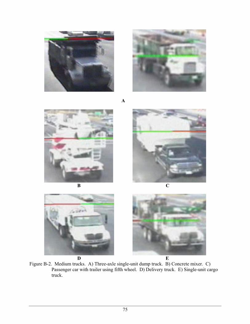
75
A
B C
D E Figure B-2. Medium trucks. A) Three-axle single-unit dump truck. B) Concrete mixer. C)
Passenger car with trailer using fifth wheel. D) Delivery truck. E) Single-unit cargo truck.
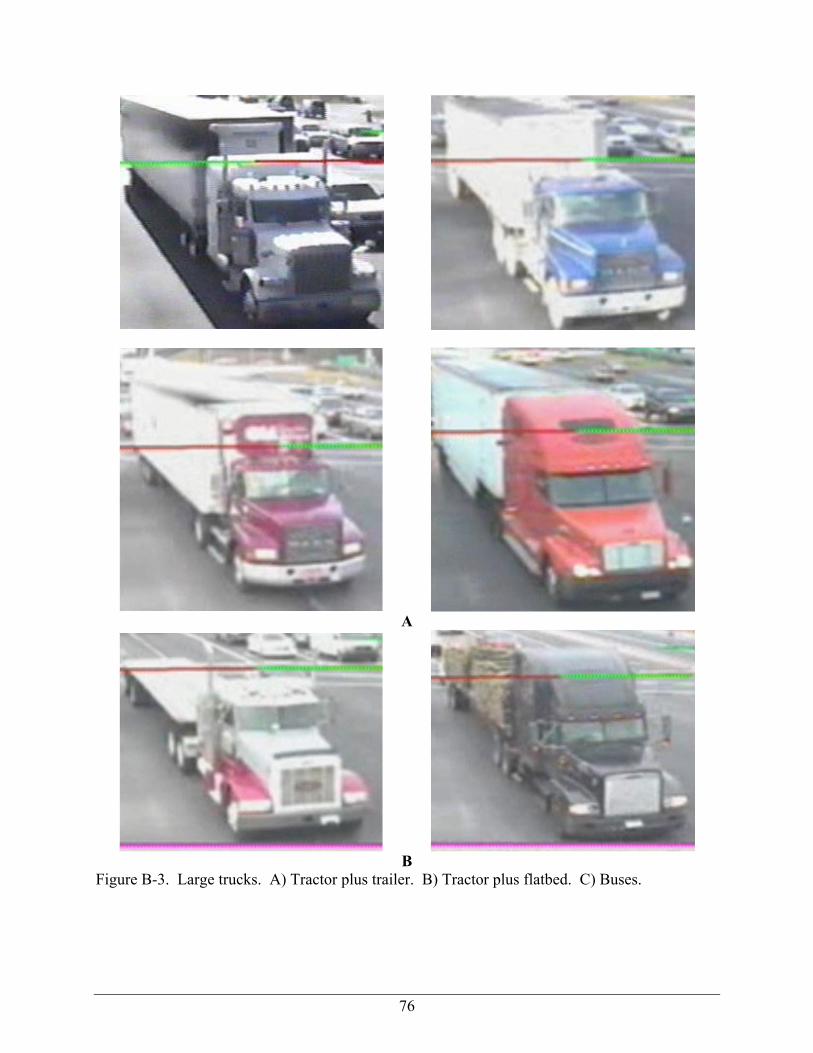
76
A
B
Figure B-3. Large trucks. A) Tractor plus trailer. B) Tractor plus flatbed. C) Buses.

77
C Figure B-3. Continued

78
APPENDIX C FLAGSIM USERS GUIDE

FlagSim User Guide Simulation Program for Two-Lane Roadways with a Lane Closure under Flagging Control
Dr. Scott Washburn University of Florida
Department of Civil and Coastal Engineering
January 2014
FlagSim User Guide January 2014
University of Florida i Transportation Institute
Table of Contents
Introduction to FlagSim .................................................................................................................. 1
Menu Items ...................................................................................................................................... 1
File ............................................................................................................................................... 1
View ............................................................................................................................................ 2
Help ............................................................................................................................................. 2
Main Inputs Screen ......................................................................................................................... 2
File Information ........................................................................................................................... 3
Roadway Information .................................................................................................................. 4
Roadway Variables ..................................................................................................................... 4
Traffic Variables ......................................................................................................................... 5
Vehicle Composition (%) ............................................................................................................ 5
Vehicle Arrivals Distribution ...................................................................................................... 6
Car-Following Model ..................................................................................................................... 6
Advanced Vehicle/Driver Parameter Values Screen ...................................................................... 8
Vehicle Characteristics ................................................................................................................ 9
Driver Characteristics ................................................................................................................ 10
Results Calculations Variables .................................................................................................. 11
Flagging Control Variables ....................................................................................................... 12
Simulation Control Panel .......................................................................................................... 18
Animation Screen .......................................................................................................................... 22
Run Control ............................................................................................................................... 23
Vehicle Tracker ......................................................................................................................... 24
Results Screen ............................................................................................................................... 25

FlagSim User Guide January 2014
University of Florida ii Transportation Institute
Output Parameters and Equations ............................................................................................. 25
Multi-Run Capability .................................................................................................................... 31
References ..................................................................................................................................... 34
APPENDIX A Vehicle Dynamics Approach to Truck Acceleration Modeling in FlagSim: Example Calculation ....................................................................................................................... 1

FlagSim User Guide January 2014
University of Florida 1 Transportation Institute
IntroductiontoFlagSimFlagSim is a Windows-based computer simulation program developed at the University of Florida Transportation Institute for the purpose of research and analysis of two-lane, two-way work zones under flagging or signal control (as illustrated in Fig. 1). This program utilizes a stochastic, microscopic modeling approach. It explicitly models the movement of every vehicle through the specified lengths of roadway, at a 0.1-second simulation time resolution.
It is not meant or designed to be used for other roadway/work zone configurations, and is designed only for operations utilizing flagging or signal control, without a pilot car. This user guide explains the inputs, how to run the simulation, and the outputs.
Figure 1. Work zone configuration to which FlagSim applies
MenuItems
File
Open
To open an existing file, select “Open” or press Ctrl+O on the keyboard.
Save/Save As
To save progress on a current file, select “Save” to save to an existing file or press Ctrl+S on the keyboard. Choose “Save As” in order to save the file under a different location or to a different name. Note that only the input data are saved to this file. The results are created in another file, as explained later.
Exit
To exit the FlagSim program, select “Exit” or click the “X” in the top right corner of the program window.

FlagSim User Guide January 2014
University of Florida 2 Transportation Institute
View
Inputs
To display the “Inputs” tab; enter all appropriate numerical inputs here.
Results
To display the summarized output file produced by FlagSim.
Help
Users Guide
This selection opens this document. This can also be accomplished by pressing Ctrl+F1 on the keyboard.
About
This selection opens the program information window.
MainInputsScreenThis screen (see Fig. 2) facilitates the setting of the values for the roadway variables, traffic variables, results calculation variables, and flagging control variables. Information on the screen should generally be entered from left to right.

FlagSim User Guide January 2014
University of Florida 3 Transportation Institute
Figure 2. Inputs screen.
File Information
File Name
Displays the name of the file for this project after it has been saved to disk. This field is not user-editable.
Analyst
Field for entering the name of the analyst.
Analysis Date
Field for entering the date of analysis. Defaults to current date.
Agency
Field for entering the name of the agency for which the analyst works.
Notes
Field for entering any additional information.

FlagSim User Guide January 2014
University of Florida 4 Transportation Institute
Roadway Information
Road Name
Field for entering the name of the roadway being analyzed.
Direction 1
The chosen direction of travel to assign to direction 1.
Direction 2
The chosen direction of travel to assign to direction 2.
Roadway Variables
Approach Roadway Length
This input specifies the length of roadway preceding the lane closure area (i.e., work zone). This is the length of roadway where vehicles approach the work zone, and subsequently accommodate storage of queued vehicles waiting to enter the work zone. The minimum and maximum input values are 0.1 miles and 5 miles, respectively. To obtain accurate queue delay and queue length estimates, the specified approach roadway length should be longer than the longest expected maximum back of queue.
Approach Roadway Posted Speed
This input specifies the legal speed limit (in units of mi/h) that vehicles can travel on the section of roadway before and after the work zone area. The minimum and maximum input values are 25 and 70, respectively.
Roadway Grade
This input specifies the incline of the roadway, in percent. Note that for downhill grades, a value of zero should be entered.
Work Zone Length
This input specifies the length of the lane closure. The units are in miles; the minimum and maximum values are 0.1 and 10, respectively.
Field-Measured Work Zone Average Travel Speed
If an existing work zone site is being analyzed, and average travel speeds through the work zone have been measured, this checkbox should be checked. If field-measured speeds are not available, the average work zone travel speed will be estimated with the following four input variables. The minimum and maximum input values are 5 and 70, respectively.
Work Zone Posted Speed
This input assigns the legal speed limit (in units of mi/h) that vehicles can travel while traversing the work zone. The minimum and maximum input values are 25 and 70, respectively.

FlagSim User Guide January 2014
University of Florida 5 Transportation Institute
Travel Direction with Lane Closed
This input specifies the travel direction that must shift lanes when entering and exiting the work zone area.
Effective Lane Width
Narrow lane widths are considered to apply to lanes that have no, or a very narrow, shoulder and cones placed inside the lane. Medium lane widths are considered to apply to lanes that have a small shoulder and cones placed outside the lane or on the centerline. Medium lane widths also apply to lanes that have a relatively wide shoulder and cones placed inside the lane. Wide lane widths are considered to apply to lanes with a relatively wide shoulder and cones placed outside the lane or on the centerline. Wide lane widths also apply to lanes that have a narrow shoulder but cones placed outside the lane.
Construction Activity
Low construction activity is considered to apply for activities such as sodding, shoulder work, or any other activity that requires few construction vehicles or equipment to operate close to the open travel lane. Medium construction activity is considered to apply for activities such as milling or resurfacing or any other activity that requires several construction vehicles or pieces of equipment to operate close to the open travel lane. High construction activity is considered to apply for activities such as both milling and resurfacing taking place at the same time or any other activity that requires a large number of construction vehicles or equipment to operate close to the open travel lane.
Advanced Work Zone Setup (Feature Forthcoming)
This feature will allow the user to adjust settings pertaining to the configuration of the work zone and approach roadways.
Traffic Variables This section of inputs allows the user to enter specific traffic flow parameters pertinent to the roadway being simulated.
Vehicle Arrival Rate
The total number of vehicles entering the network during the analysis hour (per direction, 1 and 2). Note that a “vehicle” includes both passenger cars and trucks. The minimum and maximum input values are 10 and 2000 veh/h, respectively.
Vehicle Composition (%) FlagSim has the capability to model passenger cars and three different sized trucks. The percentage of small, medium, and large trucks present in the traffic stream can be specified. The percentage of passenger cars is calculated.

FlagSim User Guide January 2014
University of Florida 6 Transportation Institute
Percent Small Trucks
This input specifies the percentage of small-sized trucks in the traffic stream.
Percent Medium Trucks
This input specifies the percentage of medium-sized trucks in the traffic stream,
Percent Large Trucks
This input specifies the percentage of large–sized trucks in the traffic stream.
Percent Passenger Cars
The percentage of passenger cars is determined implicitly from the percentage of heavy vehicles (HV). Note that the passenger cars category includes SUVs, pickup trucks, minivans, etc.
Note: The length of each vehicle type, as well as its performance capabilities (acceleration and deceleration) can be modified in the advanced vehicle/driver parameters screen.
Vehicle Arrivals Distribution This input (a drop down list box) specifies the vehicle arrival headway distribution. The two headway options are:
Negative Exponential: Arrivals are assumed to be random (i.e., according to a Poisson distribution).
Uniform: The headway between consecutive vehicle arrivals is a constant value.
The default setting is ‘negative exponential’. Thus, the vehicle arrival headway times are generated according to Eq. 1.
ln( )h r [1]
where
h = vehicle headway, in seconds r = random number generated from a uniform distribution
= average arrival rate, in veh/s ln = natural logarithm
Car‐FollowingModelThe car-following model is the mathematical foundation for the movement of a vehicle
following another vehicle. The queue discharge aspect of traffic flow in the work zone area is a critical element to the validity of the simulation results. Therefore, the car-following model has
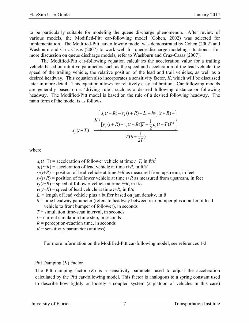
FlagSim User Guide January 2014
University of Florida 7 Transportation Institute
to be particularly suitable for modeling the queue discharge phenomenon. After review of various models, the Modified-Pitt car-following model (Cohen, 2002) was selected for implementation. The Modified-Pitt car-following model was demonstrated by Cohen (2002) and Washburn and Cruz-Casas (2007) to work well for queue discharge modeling situations. For more discussion on queue discharge models, refer to Washburn and Cruz-Casas (2007).
The Modified-Pitt car-following equation calculates the acceleration value for a trailing vehicle based on intuitive parameters such as the speed and acceleration of the lead vehicle, the speed of the trailing vehicle, the relative position of the lead and trail vehicles, as well as a desired headway. This equation also incorporates a sensitivity factor, K, which will be discussed later in more detail. This equation allows for relatively easy calibration. Car-following models are generally based on a ‘driving rule’, such as a desired following distance or following headway. The Modified-Pitt model is based on the rule of a desired following headway. The main form of the model is as follows.
2
( ) ( ) ( )
1[ ( ) ( )] ( )
2( )1
( )2
l f l f
f l l
f
s t R s t R L hv t RK
v t R v t R T a t T Ta t T
T hT
where
af (t+T) = acceleration of follower vehicle at time t+T, in ft/s2 al (t+R) = acceleration of lead vehicle at time t+R, in ft/s2 sl (t+R) = position of lead vehicle at time t+R as measured from upstream, in feet sf (t+R) = position of follower vehicle at time t+R as measured from upstream, in feet vf (t+R) = speed of follower vehicle at time t+R, in ft/s vl (t+R) = speed of lead vehicle at time t+R, in ft/s Ll = length of lead vehicle plus a buffer based on jam density, in ft h = time headway parameter (refers to headway between rear bumper plus a buffer of lead
vehicle to front bumper of follower), in seconds T = simulation time-scan interval, in seconds t = current simulation time step, in seconds R = perception-reaction time, in seconds K = sensitivity parameter (unitless)
For more information on the Modified-Pitt car-following model, see references 1-3.
Pitt Damping (K) Factor
The Pitt damping factor (K) is a sensitivity parameter used to adjust the acceleration calculated by the Pitt car-following model. This factor is analogous to a spring constant used to describe how tightly or loosely a coupled system (a platoon of vehicles in this case)

FlagSim User Guide January 2014
University of Florida 8 Transportation Institute
operates. This factor essentially adjusts how quickly or slowly acceleration changes, for one or more vehicles, propagate through the platoon.
The sensitivity parameter, K, has two separate values in the car-following model—one for the queue arrival and discharge and for the travel through the work zone. Cohen stated that a larger K value should be used in interrupted flow conditions (a more tightly coupled system) due to over-damping effects (Cohen, 2002a). This assumption was tested in the car-following model and yielded the best results. Vehicles had a smoother interaction in the work zone (uninterrupted flow, a more loosely coupled system) with K = 0.75 and for the queue arrival and queue discharge processes performed well with K = 1.1. The definition of the queue arrival area was 300 feet upstream of the last vehicle in queue, and the definition of the queue discharge area was 300 feet downstream of the entering work zone stop bar (see Figure 3).
Figure 3. Modified-Pitt K-values
AdvancedVehicle/DriverParameterValuesScreenClicking on the “Advanced Vehicle/Driver Setup…” button will open the “Vehicle and Driver Parameter Values” screen (see Fig. 4). This screen allows the user to specify the parameter values for the drivers and vehicles that enter and travel through the simulated network. Note that the default values for these parameters have been carefully chosen based on previous studies and field data collection. Unless the analyst has more specific data for a particular work zone location, it is not recommended that these values be changed. The values of these parameters can significantly affect the simulation results. Note that parameters that use a mean and standard deviation input are based on a normal distribution. Thus, approximately 68% of the parameter values will fall within +/− one standard deviation.

FlagSim User Guide January 2014
University of Florida 9 Transportation Institute
Figure 4. Vehicle and Driver Parameter Values screen.
Vehicle Characteristics Being a microscopic simulation program, FlagSim generates, moves, and tracks individual vehicles through the specified network. The following properties can be specified for each of the four vehicle types available in FlagSim.
Vehicle Length
This input specifies the length of each type of vehicle, in units of feet.
Vehicle Width
This input specifies the width of each type of vehicle, in units of feet.
Vehicle Height
This input specifies the height of each type of vehicle, in units of feet.
Vehicle Weight
This input specifies the length of each type of vehicle, in units of pounds.
Drag Coefficient
This input specifies the drag coefficient of each type of vehicle. This value is unitless.
Maximum Torque
This input specifies the maximum torque of the engine for each type of vehicle, in units of ft-lb.
FlagSim User Guide January 2014
University of Florida 10 Transportation Institute
Maximum Power
This input specifies maximum power of the engine for each type of vehicle, in units of hp.
Maximum Deceleration
This input specifies the maximum deceleration (i.e., braking) rate for each type of vehicle, in units of ft/s2.
Driver Characteristics For each individual vehicle generated during the simulation, a unique driver is attached to
the vehicle. A number of characteristics are associated with each driver. Furthermore, to allow for variance from one driver to another, values of each of the characteristics are drawn from a Normal distribution, as specified by mean and standard deviation values. Thus, the property values were set according to Eq. 2.
normValue s r x [2]
where
Value = vehicle parameter value, such as desired acceleration s = standard deviation input by the user rnorm = random normal number generated by the random normal function x = mean value of the property inputted by the user
Desired Acceleration (mean and standard deviation)
This input specifies the desired acceleration rate for a driver, in units of ft/s2. This value will be applied when a vehicle is not in a car-following mode and is traveling less than its desired speed.
Desired Deceleration (mean and standard deviation)
This input specifies the desired deceleration rate for a driver, in units of ft/s2. This deceleration rate is applied for normal braking situations, such as stopping when joining the queue at the approach to the work zone. Note that this value should be less than the maximum deceleration rate, which is used only in emergency braking situations.
Desired Speed % (mean and standard deviation)
This input specifies the percentage above (for positive values) or below (for negative values) the base desired speed that a particular driver will travel. For example, passenger car drivers will travel 7.5% above the base desired speed, on average, while large truck drivers will travel 5% below the base desired speed, on average (for the default values shown). The base desired speed value is a function of factors such as posted speed limit, construction activity, effective lane width, and direction of closed lane.

FlagSim User Guide January 2014
University of Florida 11 Transportation Institute
Headway (mean and standard deviation)
This input specifies the length of the vehicle headway (time interval between consecutive vehicles) value used in the Modified-Pitt car-following model (the h parameter).
Reaction Time (mean and standard deviation)
This input specifies the driver reaction time used in the Modified-Pitt car-following model (the R parameter).
Stop Gap (mean and standard deviation)
This input specifies the distance, in units of feet, between the rear bumper of a lead vehicle and the front bumper of a trail vehicle, while at a stop (i.e., in a queue waiting to enter the work zone). This value combined with the vehicle length value comprises the L parameter used in the Modified-Pitt car-following model.
Note that maximum acceleration is not an input to FlagSim. This value is determined explicitly by FlagSim for every vehicle at every simulation time step. More information about the maximum acceleration modeling approach utilized in FlagSim can be found in Appendix A.
The ‘Modified-Pitt Damping Factor’ inputs pertain to the car-following model employed in FlagSim. These inputs are discussed in more detail in the previous section.
It is not recommended that any of the above values be changed unless the analyst has
specific data for a site contrary to these values.
Results Calculations Variables Time delay accumulates when drivers are forced to travel under the specified speed limit or their desired free flow speed. The following two parameters allow the user to specify speeds that are considered “time-delay” to motorists – whether in a queue or traveling through the work zone at a speed lower than the posted speed limit.
Work Zone Travel Delay Threshold Speed
This input specifies the speed threshold for which delay for vehicles traveling through the work zone is accumulated. The average speed is calculated for every vehicle traveling through the work zone. If this average speed is below the speed threshold, it will have travel time delay calculated for it. Minimum and maximum input values are 5 mi/h and 70 mi/h, respectively.
Queue Delay Threshold Speed
This input specifies the speed threshold for which delay for vehicles approaching the work zone is accumulated. For example, if the threshold speed is 10 mi/h, for every time step (i.e., 0.1 seconds during the simulation) that a vehicle’s speed is below this speed, it accumulates queue delay. Note that a queue threshold speed of 0 mi/h would be

FlagSim User Guide January 2014
University of Florida 12 Transportation Institute
considered to be just stop delay. A higher value will also account for the delay accumulated while moving up in a queue (at slow speed) and some of the time decelerating to join the back of queue or re-accelerating from a queue to enter the work zone. Generally, the threshold speed accounts for the all the delays tallied from a queue listed previously. Minimum and maximum input values are 0 mi/h and 15 mi/h, respectively.
Flagging Control Variables The “Flagging Control” variables section of the inputs window allows the user to first specify how the traffic volumes using the work zone will be controlled. Then, the user can specify the values of the applicable parameters for the chosen right-of-way allocation method.
Flagging Control
Four flagging control methods are available for use in FlagSim:
Fixed Time
Distance Gap Out
Time Gap Out
Maximum Queue Length

FlagSim User Guide January 2014
University of Florida 13 Transportation Institute
Fixed Time
The “Fixed Time” flagging control method assigns a fixed amount of green time to each direction, as specified in the “Max Green Time” input. Minimum and maximum values for mean max green time are 5 seconds and 300 seconds, respectively. The standard deviation for this input can also be adjusted by the user to allow for randomness in the actual green times applied by the flag person. A non-zero standard deviation would more realistic for human flaggers. Maximum and minimum standard deviation values are 0 seconds and 10 seconds, respectively.
Time Gap Out
The “Time Gap Out” flagging method keeps green time assigned to a given direction until the time elapsed between the last vehicle to enter the work zone and the next approaching vehicle exceeds the specified gap-out time. The minimum and maximum mean gap-out times are 0 seconds and 50 seconds, respectively. Minimum and maximum standard deviations are 0 seconds and 10 seconds, respectively.
Minimum and maximum green times are also applicable in this control mode, and take priority over the gap-out time. These minimum and maximum values are 5 seconds and 300 seconds, respectively. Note that the minimum green time can be automatically computed based upon the method given in reference 1. To have the minimum green time calculated, simply click on the “Calculate Minimum Green Time” button.

FlagSim User Guide January 2014
University of Florida 14 Transportation Institute
Distance Gap Out
The “Distance Gap Out” flagging method keeps green time assigned to a given direction until the distance between the last vehicle to enter the work zone and the next approaching vehicle exceeds the specified gap-out distance. The minimum and maximum mean gap-out distances are 20 feet and 1200 feet, respectively. A non- zero standard deviation can be applied to the mean distance gap out. Although a clear gap out zone can be marked by an orange cone or striped line across the road, the flag person may have a difficult time accurately depicting whether or not a vehicle has entered the gap out zone. Hence, a non-zero standard deviation would better simulate such flagging conditions. Minimum and maximum standard deviations are 0 ft and 50 ft, respectively.
Minimum and maximum green times are also applicable in this control mode, and take priority over the gap-out distance. These minimum and maximum values are 5 seconds and 300 seconds, respectively. Note that the minimum green time can be automatically computed based upon the method given in reference 1. To have the minimum green time calculated, simply click on the “Calculate Minimum Green Time” button.
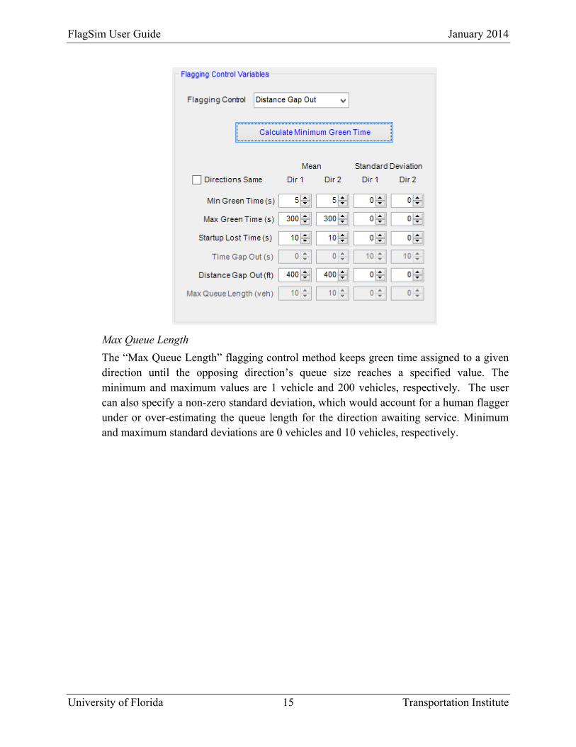
FlagSim User Guide January 2014
University of Florida 15 Transportation Institute
Max Queue Length
The “Max Queue Length” flagging control method keeps green time assigned to a given direction until the opposing direction’s queue size reaches a specified value. The minimum and maximum values are 1 vehicle and 200 vehicles, respectively. The user can also specify a non-zero standard deviation, which would account for a human flagger under or over-estimating the queue length for the direction awaiting service. Minimum and maximum standard deviations are 0 vehicles and 10 vehicles, respectively.

FlagSim User Guide January 2014
University of Florida 16 Transportation Institute
Minimum and maximum green times are also applicable in this control mode, and take priority over the max queue length. These minimum and maximum values are 5 seconds and 300 seconds, respectively. Note that the minimum green time can be automatically computed based upon the method given in reference 1. To have the minimum green time calculated, simply click on the “Calculate Minimum Green Time” button.
Other Inputs
Startup Lost Time
Mean
This input specifies the average time, in seconds, that elapses between when the last vehicle in one direction exits the work zone and when the first queued vehicle in the other direction enters the work zone. The default value is 10 seconds. Minimum and maximum values for both directions are 1 second and 20 seconds, respectively.
Standard Deviation
The standard deviation for the startup lost time can also be specified in order to account for natural phase-to-phase randomness in this value. The randomness occurs from a difference in both the time it takes the flag person to turn the paddle to “Slow” after the last vehicle exits the work zone and the time it takes the first queued vehicle to startup and enter the work zone once the flag person turns the paddle to “Slow.” It should be noted that the position of the flag person and the beginning of work zone are assumed to

FlagSim User Guide January 2014
University of Florida 17 Transportation Institute
be at the same location, which is also where the first vehicle in queue stops in FlagSim. In the field, however, it is more typical that the first vehicle in queue stops 2-3 car lengths upstream of the flag person/work zone entry point. Thus, in FlagSim, the entry of the first vehicle in queue into the work zone and the changing of the flag paddle to “Slow” happen at the same time. In the field, the first vehicle usually enters the work zone a couple of seconds after the flag person turns the paddle to “Slow”. Thus, it is important that any field-measured lost times include the additional 2-3 seconds that it usually takes the first vehicle in queue to reach the work zone entry point after the flag paddle is turned “Slow”.
Directions Same Checkbox
Checking this box disables the inputs for direction 2 and applies the input values for direction 1 to both directions.
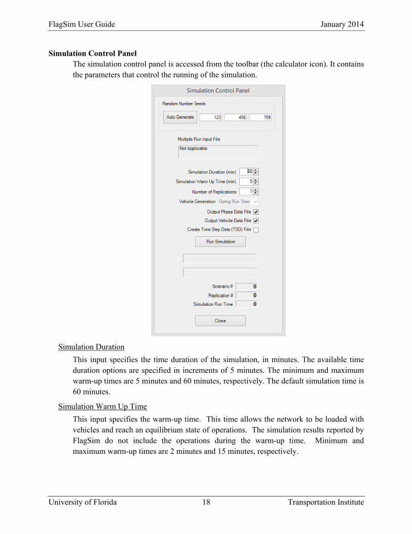
FlagSim User Guide January 2014
University of Florida 18 Transportation Institute
Simulation Control Panel The simulation control panel is accessed from the toolbar (the calculator icon). It contains the parameters that control the running of the simulation.
Simulation Duration
This input specifies the time duration of the simulation, in minutes. The available time duration options are specified in increments of 5 minutes. The minimum and maximum warm-up times are 5 minutes and 60 minutes, respectively. The default simulation time is 60 minutes.
Simulation Warm Up Time
This input specifies the warm-up time. This time allows the network to be loaded with vehicles and reach an equilibrium state of operations. The simulation results reported by FlagSim do not include the operations during the warm-up time. Minimum and maximum warm-up times are 2 minutes and 15 minutes, respectively.
FlagSim User Guide January 2014
University of Florida 19 Transportation Institute
Number of Replications
The input specifies the number of times a given set of input conditions will be simulated. The random number seeds will be changed with each subsequent run.
Vehicle Generation
This feature is currently disabled.
Output Data Files
The output data files are generated for the simulation if the user checks the corresponding boxes. These files are written to the folder where FlagSim is installed, and are in a comma-separated values (CSV) format. Thus, they can easily be opened in the Microsoft Excel program. The data file for direction 1 is designated with a “1”, while the data file for direction 2 is designated with a “2”. Note that times reported in these files are in units of tenths of seconds.
Phase Data File
This output file summarizes data results for each phase (i.e., start of green to end of green). This file gives information such fields as the beginning and ending vehicle per phase; the time (in tenths of a second) at the start and end of green; the queue (number of vehicles lined up waiting to enter the work zone) at the onset of each green phase, the time when the maximum queue occurs, the maximum back of queue (the distance, in feet, from the stop bar to the rear bumper of the last car in the queue for a given phase); the amount of time spent delayed in the queue, and the average work zone speed. Note that the work zone speed is given in units of miles per hour. These parameters are specified for each direction (1 and 2). Separate CSV files are generated for each direction: “PhaseData_Dir_1 or PhaseData_Dir_2.”
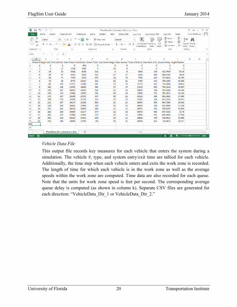
FlagSim User Guide January 2014
University of Florida 20 Transportation Institute
Vehicle Data File
This output file records key measures for each vehicle that enters the system during a simulation. The vehicle #, type, and system entry/exit time are tallied for each vehicle. Additionally, the time step when each vehicle enters and exits the work zone is recorded. The length of time for which each vehicle is in the work zone as well as the average speeds within the work zone are computed. Time data are also recorded for each queue. Note that the units for work zone speed is feet per second. The corresponding average queue delay is computed (as shown in column k). Separate CSV files are generated for each direction: “VehicleData_Dir_1 or VehicleData_Dir_2.”
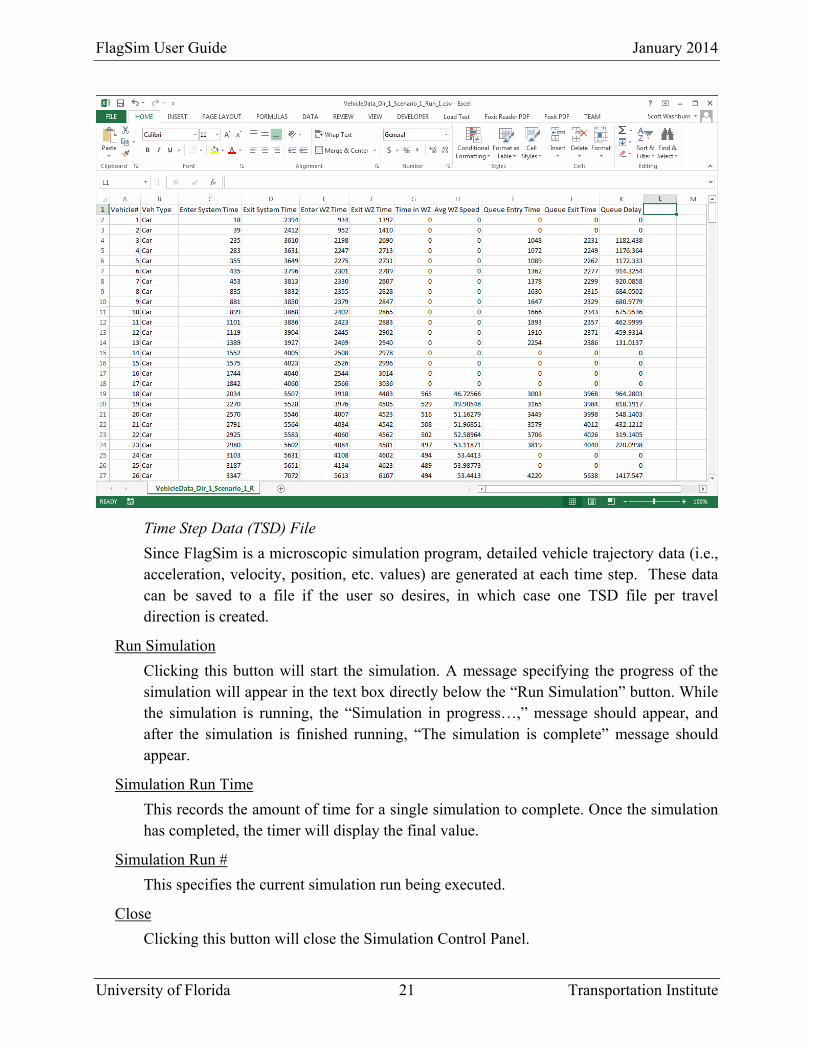
FlagSim User Guide January 2014
University of Florida 21 Transportation Institute
Time Step Data (TSD) File
Since FlagSim is a microscopic simulation program, detailed vehicle trajectory data (i.e., acceleration, velocity, position, etc. values) are generated at each time step. These data can be saved to a file if the user so desires, in which case one TSD file per travel direction is created.
Run Simulation
Clicking this button will start the simulation. A message specifying the progress of the simulation will appear in the text box directly below the “Run Simulation” button. While the simulation is running, the “Simulation in progress…,” message should appear, and after the simulation is finished running, “The simulation is complete” message should appear.
Simulation Run Time
This records the amount of time for a single simulation to complete. Once the simulation has completed, the timer will display the final value.
Simulation Run #
This specifies the current simulation run being executed.
Close
Clicking this button will close the Simulation Control Panel.

FlagSim User Guide January 2014
University of Florida 22 Transportation Institute
AnimationScreenFlagSim incorporates a 2-D post-processor animation viewer, shown in the figure below.
The animation allows the user to view the computations previously performed. Viewing the animation gives the user an opportunity to review the simulation scenario visually. Items that can be easily checked are vehicle generation, car-following interaction, and the flagging operations.
Click on the right-most button on the toolbar. This displays the work zone simulation animation. The work zone stop bars (also assumed to be the flagger position) are identified with green, yellow, and red vertical bars (i.e., running perpendicular to the roadway). The color of the stop bar indicates which direction will have or has the right-of-way. Yellow indicates the start-up lost time for a given phase.
Passenger cars are shown in blue, small trucks in purple, medium trucks in green, and large trucks in red. Since the animation can cover a significant length of roadway, the display of the roadway is presented in a stacked fashion to utilize the full screen area and avoid a lot horizontal scrolling. Thus, a vehicle that disappears off the edge of the screen on one side will reappear on the other side of the screen (except for vehicles exiting the system), one level higher or lower, depending on the direction of vehicle movement. This also allows most of the roadway network to be observed in its entirety for many roadway configurations.
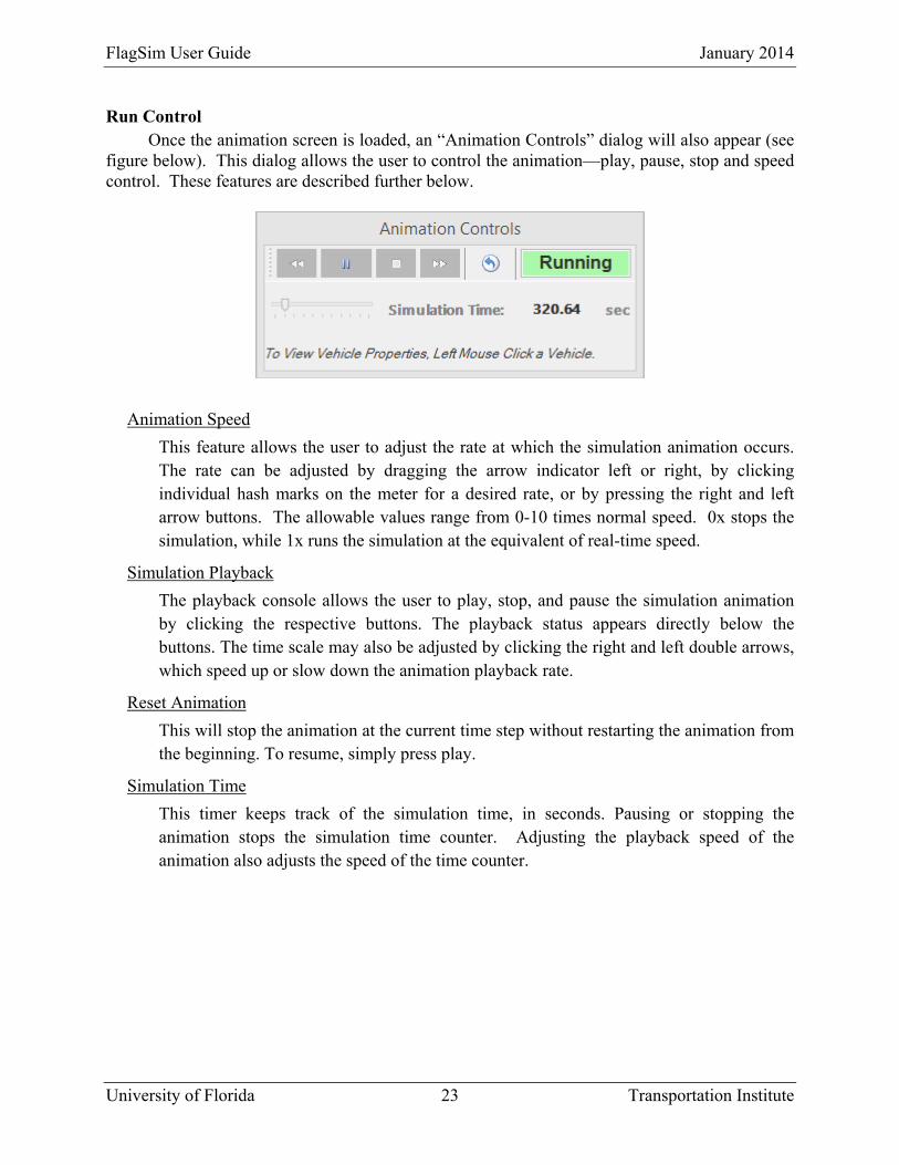
FlagSim User Guide January 2014
University of Florida 23 Transportation Institute
Run Control Once the animation screen is loaded, an “Animation Controls” dialog will also appear (see
figure below). This dialog allows the user to control the animation—play, pause, stop and speed control. These features are described further below.
Animation Speed
This feature allows the user to adjust the rate at which the simulation animation occurs. The rate can be adjusted by dragging the arrow indicator left or right, by clicking individual hash marks on the meter for a desired rate, or by pressing the right and left arrow buttons. The allowable values range from 0-10 times normal speed. 0x stops the simulation, while 1x runs the simulation at the equivalent of real-time speed.
Simulation Playback
The playback console allows the user to play, stop, and pause the simulation animation by clicking the respective buttons. The playback status appears directly below the buttons. The time scale may also be adjusted by clicking the right and left double arrows, which speed up or slow down the animation playback rate.
Reset Animation
This will stop the animation at the current time step without restarting the animation from the beginning. To resume, simply press play.
Simulation Time
This timer keeps track of the simulation time, in seconds. Pausing or stopping the animation stops the simulation time counter. Adjusting the playback speed of the animation also adjusts the speed of the time counter.
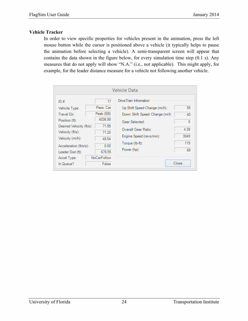
FlagSim User Guide January 2014
University of Florida 24 Transportation Institute
Vehicle Tracker In order to view specific properties for vehicles present in the animation, press the left mouse button while the cursor is positioned above a vehicle (it typically helps to pause the animation before selecting a vehicle). A semi-transparent screen will appear that contains the data shown in the figure below, for every simulation time step (0.1 s). Any measures that do not apply will show “N.A.” (i.e., not applicable). This might apply, for example, for the leader distance measure for a vehicle not following another vehicle.

FlagSim User Guide January 2014
University of Florida 25 Transportation Institute
ResultsScreenOnce a simulation run is complete, the overall results for the simulation period can be accessed by clicking on the tab in the lower right corner of the screen.
This window provides a summary of the key performance measures for the work zone operation, such as total system delay, maximum queue length, average delay in work zone, etc. This file is written to the same folder that contains the FlagSim program. It can be loaded into any text editing program for further formatting and/or printing.
Output Parameters and Equations This section describes each of the measures provided in the results file. The equations used to calculate each of the output values, as appropriate, are also described.
System Entry Volume — number of vehicles entering the system for the simulation time period Note that the system entry volume can be smaller than the work zone entry volume. This happens if a vehicle enters the system before the end of the warm-up period but enters the work zone after the warm-up period ends (excludes warm-up period).

FlagSim User Guide January 2014
University of Florida 26 Transportation Institute
Work Zone Entry Volume — number of vehicles entering the work zone for the simulation time period (excludes warm-up period).
Work Zone Exit Volume — number of vehicles exiting the work zone for the simulation time period. Note that the work zone exit volume can be smaller than the work zone entry volume. This happens if the simulation time period expires while some vehicles are still present in the work zone (excludes warm-up period).
Average Time in Work Zone —average travel time through the work zone for all vehicles traveling inside the work zone area. It is calculated according to the following equation.
_1
__ _
_ = average travel time through the work zone for vehicles traveling in direction k, in
seconds _ _ = travel time through work zone for vehicle i in direction k, in seconds
= time vehicle i exits work zone time vehicle i enters work zone x = the first vehicle to enter the work zone in direction k after the simulation warm-up period
has ended y = the last vehicle to exit the work zone in direction k after the simulation warm-up period
has ended i = vehicle number k = travel direction (1 or 2) nveh_k = total number of vehicles to traverse the work zone in direction k after the simulation
warm-up period has ended in direction
Average Speed in Work Zone —average speed of all vehicles traveling inside the work zone area. It is calculated according to the following equation.
_1
_ _ _ 3600⁄
_ = average vehicle speed in the work zone for direction k, in mi/h WZlength = work zone length, in miles
Average Delay in Work Zone — average travel time delay experienced by all vehicles while within the work zone.

FlagSim User Guide January 2014
University of Florida 27 Transportation Institute
_
1
__ _
_ = average work zone delay for vehicles traveling in direction k, in seconds
_ _ = work zone delay for vehicle i traveling in direction k, in seconds = _ _
BaseWZTravTime = travel time through work zone if traveling at “Work Zone Travel Delay Threshold Speed” (WZdelspd) in seconds
= ⁄ 3600⁄ WZdelspd = travel speed below which work zone travel delay accumulates (default is work
zone posted speed), in mi/h
Average Delay in Queue — average travel time delay experienced by all vehicles while in queue. Queue delay for an individual vehicle is obtained by adding a second of delay for every second the vehicle is traveling at a speed below the “Queue Delay Threshold Speed.” The default “Queue Delay Threshold Speed” is 10 mi/h.
_
1
__ _
_ = average queue delay for vehicles traveling in direction k, in seconds
_ _ = queue delay for vehicle i traveling in direction k, in seconds
Total Delay in Work Zone — total travel time delay experienced by all vehicles while within the work zone.
_ _ _ _ 3600⁄
_ _ = total work zone delay for all vehicles traveling in direction k, in hours
Total Delay in Queue — total travel time delay experienced by all vehicles while in queue.
_ _ _ _ 3600⁄
_ _ = total queue delay for all vehicles traveling in direction k, in hours

FlagSim User Guide January 2014
University of Florida 28 Transportation Institute
Total Delay per Direction — total travel time delay (sum of Total Delay in Work Zone and Total Delay in Queue) experienced by all vehicles for a given direction for the simulation time period.
_ _ _ _ _
_ = total delay for all vehicles traveling in direction k, in hours
Total System Delay — total travel time delay (sum of Total Delay for both directions) experienced by all vehicles traversing the work zone during the simulation time period (excluding the warm-up time).
_ _
_ = total delay for all vehicles that traverse the work zone, traveling in direction k, during the simulation time period (excluding the warm-up time), in hours
Average Queue Size at Beginning of Green — the average number of vehicles in queue per phase measured at the time when the flag indication turns to green.
_1
__ _
_ = average queue size per phase at the beginning of green period for direction k, in vehicles
_ _ = queue size at the beginning of green period for phase j in direction k, in vehicles a = the first phase to occur in direction k after the simulation warm-up period has ended b = the last phase to occur in direction k after the simulation warm-up period has ended j = phase number nphase_k = total number of phases that occur for direction k after the simulation warm-up
period has ended
Average Maximum Queue Size — the average number of vehicles in queue per phase measured at the time when the queue is largest. It should be noted that the queue size used for each phase is the absolute maximum queue, which accounts for vehicles arriving on green at the back of the initial queue at the start of green.
_1
__ _
_ = average maximum queue size per phase for direction k, in vehicles
_ _ = maximum queue size for phase j in direction k, in vehicles

FlagSim User Guide January 2014
University of Florida 29 Transportation Institute
Maximum Queue Size — the maximum number of vehicles in queue during the entire simulation period; that is, across all phases.
_ max _ _
_ = maximum queue size across all phases for direction k, in vehicles
Maximum Back of Queue — the distance corresponding to the maximum queue size, _ .
This distance is calculated by taking the difference between the position of the stop bar for direction k and the position of the back bumper of the last vehicle in queue. This value is reported in feet.
Average Green per Phase — the average green period per phase where the green period is the elapsed time between when the flag indication turns to green and when it turns back to red. It should be noted that if the green period of the last phase to occur after the warm-up period has ended, phase b, does not terminate before the end of the simulation period this phase is not included in the calculation. In this case the phase prior to this phase is used as phase b.
1
__
= average green period per phase for direction k, in seconds _ = green period for phase j in direction k, in seconds
= _ _ _ _
_ _ = time flag indication turns to red to end phase j in direction k, in seconds after simulation began
_ _ = time flag indication turns to green to begin phase j in direction k, in seconds after simulation began
Average Cycle Length — the average cycle length, calculated simply as the sum of all cycle lengths divided by the number of cycles in the simulation period. Cycle length is measured as the time elapsed between the beginning of green for one phase and direction and the beginning of green for the next phase in the same direction.
1_

FlagSim User Guide January 2014
University of Florida 30 Transportation Institute
= average cycle length for direction k, in seconds _ = cycle length corresponding to phase j in direction k, in seconds
= _ _ _ _ ncycle = total number of cycles that occur after the simulation warm-up period has ended
Average g/C — the average green period to cycle length ratio. It is calculated according to the following formula.
1 _
_
= average green period to cycle length ratio for direction k, unitless

FlagSim User Guide January 2014
University of Florida 31 Transportation Institute
Multi‐RunCapabilityTo facilitate multiple runs for different scenarios (i.e., different sets of inputs), the user can
choose to open a Multi-Run File from the FlagSim open dialog screen.
The multi-run file must be in a comma-separated values (i.e., “*.csv”) format and have the FlagSim inputs arranged in a specific way. The first row is used to label the FlagSim inputs, but is not read by the program. This simply provides the user with a reference as to which column corresponds to which FlagSim input. The second and subsequent rows are used to assign the FlagSim input values for the different scenarios. Each row is a separate scenario. Therefore, the inputs in row 2 are for scenario 1, and the inputs in row 3 are for scenario 2, etc. This is done for as many scenarios as one wishes to run. The FlagSim inputs should be placed in the .csv file in the following order with the corresponding column letters (per Microsoft Excel’s column labeling scheme, other programs may vary).
A. Scenario # — the scenario number corresponding to the row of inputs B. AppLength — approach roadway length, in miles C. WZLength — length of the work zone, in miles D. AppSpeed_Dir1 — approach roadway posted speed for direction 1, in mi/h E. AppSpeed_Dir2 — approach roadway posted speed for direction 2, in mi/h F. GradeProp_Dir1 — roadway grade for direction 1, expressed as a proportion
FlagSim User Guide January 2014
University of Florida 32 Transportation Institute
G. GradeProp_Dir2 — roadway grade for direction 2, expressed as a proportion H. WZMeasSpeed — average speed (or other appropriate percentile speed, at discretion of
analyst) through the work zone measured from the field (if speed was not measured, use value of 0), in mi/h
I. WZPostSpeed — posted speed in the work zone area, in mi/h J. EstSpeed? — is the work zone speed estimated? (use value of “Yes” if using
“WZPostSpeed” for simulation and “No” if using “WZMeasSpeed”) K. EffLaneWidth — effective lane width in work zone (use value of “Narrow” for narrow
lane width, “Med” for medium lane width, and “Wide” for wide lane width) L. ConstAct — level of construction activity in work zone (use value of “Low” for no or
low construction activity, “Med” for medium construction activity, and “High” for high construction activity)
M. DirClose — specifies which travel direction has the closed lane (use value of “Dir1” if the lane for direction 1 is closed and value of “Dir2” if the lane for direction 2 is closed)
N. WZDelaySpeed — speed threshold used to calculate travel time delay of vehicles in the work zone. Vehicles accumulate work zone delay when traveling at a speed below this threshold. Set “WZDelaySpeed” equal to “WZMeasSpeed” or “WZPostSpeed,” unless it is desirable to use a different speed. Value should be in mi/h.
O. QueueDelaySpeed — speed threshold used to calculate travel time delay of vehicles in queue. Vehicles accumulate queue delay when traveling at a speed below this threshold. Set QueueDelaySpeed equal to 10, unless there is a reason to use a different speed. Value should be in mi/h.
P. PctCar_Dir1 — percentage of passenger cars traveling in direction 1 Q. PctST_Dir1 — percentage of small trucks traveling in direction 1 R. PctMT_ Dir1 — percentage of medium trucks traveling in direction 1 S. PctLT_ Dir1 — percentage of large trucks traveling in direction 1 T. PctCar_ Dir2 — percentage of passenger cars traveling in direction 2 U. PctST_ Dir2 — percentage of small trucks traveling in direction 2 V. PctMT_ Dir2 — percentage of medium trucks traveling in direction 2 W. PctLT_ Dir2 — percentage of large trucks traveling in direction 2 X. Vol_Dir1 — vehicle arrival rate for direction 1, in veh/h Y. Vol_Dir2 — vehicle arrival rate for direction 2, in veh/h Z. Control — type of flagging control used at the work zone (use value of “FixedTime” for
Fixed Time flagging control, “MaxQueue” for Max Queue Length flagging control, “GapOutDistance” for Distance Gap Out flagging control, and “GapOutTime” for Time Gap Out flagging control)
AA. MinGreenMean_Dir1 — mean of minimum green time for direction 1, in sec AB. MinGreenMean_Dir2 — mean of minimum green time for direction 2, in sec AC. MinGreenStdev_Dir1 — standard deviation of minimum green time for direction 1, in
sec

FlagSim User Guide January 2014
University of Florida 33 Transportation Institute
AD. MinGreenStdev_Dir2 — standard deviation of minimum green time for direction 2, in sec
AE. MaxGreenMean_Dir1 — mean of maximum green time for direction 1, in sec AF. MaxGreenMean_Dir2 — mean of maximum green time for direction 2, in sec AG. MaxGreenStdev_Dir1 — standard deviation of maximum green time for direction 1, in
sec AH. MaxGreenStdev_Dir2 — standard deviation of maximum green time for direction 2, in
sec AI. LostTimeMean_Dir1 — mean of startup lost time for direction 1, in sec AJ. LostTimeMean_Dir2 — mean of startup lost time for direction 2, in sec AK. LostTimeStdev_Dir1 — standard deviation of startup lost time for direction 1, in sec AL. LostTimeStdev_Dir2 — standard deviation of startup lost time for direction 2, in sec AM. ControlMean_Dir1 — mean of input used for flagging control for direction 1 (for “Max
Queue Length” flagging control is mean of “Max Queue Length” in vehicles, for “Distance Gap Out” flagging control is mean of “Distance Gap Out” in feet, and for “Time Gap Out” flagging control is mean of “Time Gap Out” in seconds). If using “Fixed Time” flagging control leave this input blank (fixed time uses the maximum green time inputs).
AN. ControlMean_Dir2 — mean of input used for flagging control for direction 2 (for “Max Queue Length” flagging control is mean of “Max Queue Length” in vehicles, for “Distance Gap Out” flagging control is mean of “Distance Gap Out” in feet, and for “Time Gap Out” flagging control is mean of “Time Gap Out” in seconds). If using “Fixed Time” flagging control leave this input blank (fixed time uses the maximum green time inputs).
AO. ControlStdev_Dir1 — standard deviation of input used for flagging control for direction 1 (for “Max Queue Length” flagging control is standard deviation of “Max Queue Length” in vehicles, for “Distance Gap Out” flagging control is standard deviation of “Distance Gap Out” in feet, and for “Time Gap Out” flagging control is standard deviation of “Time Gap Out” in seconds). If using “Fixed Time” flagging control leave this input blank (fixed time uses the maximum green time inputs).
AP. ControlStdev_Dir2 — standard deviation of input used for flagging control for direction 2 (for “Max Queue Length” flagging control is standard deviation of “Max Queue Length” in vehicles, for “Distance Gap Out” flagging control is standard deviation of “Distance Gap Out” in feet, and for “Time Gap Out” flagging control is standard deviation of “Time Gap Out” in seconds). If using “Fixed Time” flagging control leave this input blank (fixed time uses the maximum green time inputs).
FlagSim User Guide January 2014
University of Florida 34 Transportation Institute
References
1. Washburn, Scott S, Hiles, Thomas, and Heaslip, Kevin. Impact of Lane Closures on Roadway Capacity: Development of a Two-Lane Work Zone Lane Closure Analysis Procedure (Part A). Final Report. Florida Department of Transportation. Tallahassee, FL. January 2008.
2. Cohen, Stephen, L. (2002). Application of Car-Following Systems in Microscopic Time-Scan Simulation Models. Journal of the Transportation Research Board, TRR 1802, 239-247.
3. Cohen, Stephen, L. (2002). Application of Car-Following Systems to Queue Discharge Problem at Signalized Intersections. Journal of the Transportation Research Board, TRR 1802, 205-213.
For more information, contact:
Scott S. Washburn, Ph.D., P.E. Associate Professor University of Florida Dept. of Civil and Coastal Engineering 365 Weil Hall, Box 116580 Gainesville, FL 32611-6580 [email protected] http://www.transportation.ufl.edu/
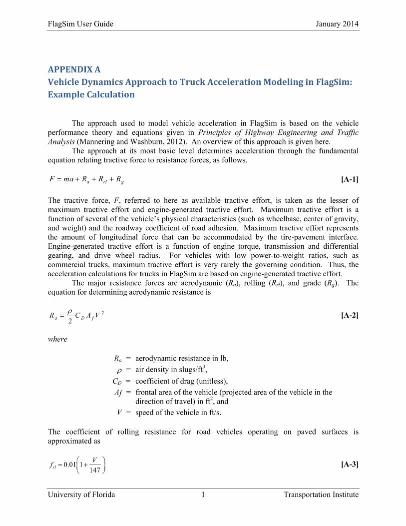
FlagSim User Guide January 2014
University of Florida 1 Transportation Institute
APPENDIXAVehicleDynamicsApproachtoTruckAccelerationModelinginFlagSim:ExampleCalculation
The approach used to model vehicle acceleration in FlagSim is based on the vehicle performance theory and equations given in Principles of Highway Engineering and Traffic Analysis (Mannering and Washburn, 2012). An overview of this approach is given here.
The approach at its most basic level determines acceleration through the fundamental equation relating tractive force to resistance forces, as follows.
a rl gF ma R R R [A-1]
The tractive force, F, referred to here as available tractive effort, is taken as the lesser of maximum tractive effort and engine-generated tractive effort. Maximum tractive effort is a function of several of the vehicle’s physical characteristics (such as wheelbase, center of gravity, and weight) and the roadway coefficient of road adhesion. Maximum tractive effort represents the amount of longitudinal force that can be accommodated by the tire-pavement interface. Engine-generated tractive effort is a function of engine torque, transmission and differential gearing, and drive wheel radius. For vehicles with low power-to-weight ratios, such as commercial trucks, maximum tractive effort is very rarely the governing condition. Thus, the acceleration calculations for trucks in FlagSim are based on engine-generated tractive effort.
The major resistance forces are aerodynamic (Ra), rolling (Rrl), and grade (Rg). The equation for determining aerodynamic resistance is
2
2a D fR C A V
[A-2]
where
Ra = aerodynamic resistance in lb,
= air density in slugs/ft3,
CD = coefficient of drag (unitless),
Af = frontal area of the vehicle (projected area of the vehicle in the direction of travel) in ft2, and
V = speed of the vehicle in ft/s. The coefficient of rolling resistance for road vehicles operating on paved surfaces is approximated as
0.01 1147rl
Vf
[A-3]
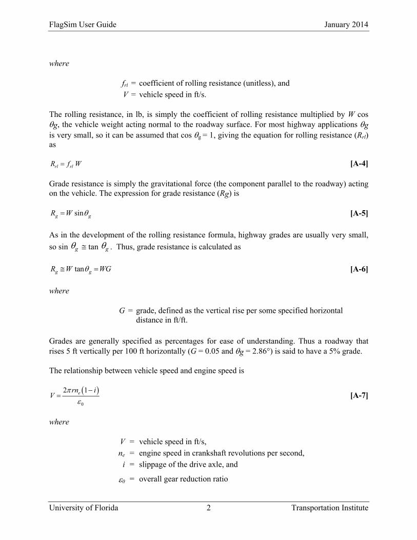
FlagSim User Guide January 2014
University of Florida 2 Transportation Institute
where
frl = coefficient of rolling resistance (unitless), and
V = vehicle speed in ft/s. The rolling resistance, in lb, is simply the coefficient of rolling resistance multiplied by W cos g, the vehicle weight acting normal to the roadway surface. For most highway applications g is very small, so it can be assumed that cos g = 1, giving the equation for rolling resistance (Rrl) as
rl rlR f W [A-4] Grade resistance is simply the gravitational force (the component parallel to the roadway) acting on the vehicle. The expression for grade resistance (Rg) is
sing gR W [A-5]
As in the development of the rolling resistance formula, highway grades are usually very small,
so sin g tan g . Thus, grade resistance is calculated as
tang gR W WG [A-6]
where
G = grade, defined as the vertical rise per some specified horizontal distance in ft/ft.
Grades are generally specified as percentages for ease of understanding. Thus a roadway that rises 5 ft vertically per 100 ft horizontally (G = 0.05 and g = 2.86°) is said to have a 5% grade. The relationship between vehicle speed and engine speed is
0
2 1ern iV
[A-7]
where
V = vehicle speed in ft/s,
ne = engine speed in crankshaft revolutions per second,
i = slippage of the drive axle, and
0 = overall gear reduction ratio

FlagSim User Guide January 2014
University of Florida 3 Transportation Institute
The overall gear reduction ratio is a function of the differential gear ratio and the transmission gear ratio, which is a function of the selected transmission gear for the running speed. This equation can be rearranged to solve for engine speed given the current vehicle speed (if vehicle speed is zero, engine speed is a function of throttle input).
With the calculated engine speed, the torque being produced by the engine can be determined from the torque-engine speed relationship. For example, assuming an engine speed of 2000 revolutions/min with the torque-engine speed relationship (Paccar PX-7 Engine) shown in Figure 5 (Ref. 3), the resulting torque is 660 ft-lb. In addition, Figure 6 shows the torque-engine speed relationship for a Paccar MX-13 engine (Ref. 4).
Figure 5. Torque-engine speed curve for a Paccar PX-7 engine
FlagSim User Guide January 2014
University of Florida 4 Transportation Institute
Figure 6. Torque-engine speed curve for a Paccar MX-13 engine
Power is the rate of engine work, expressed in horsepower (hp), and is related to the engine’s torque by the following equation:
2hp
550e e
e
πM n = [A-8]
where
hpe = engine-generated horsepower (1 horsepower equals 550 ft-lb/s),
Me = engine torque in ft-lb, and
ne = engine speed in crankshaft revolutions per second.
The engine-generated tractive effort reaching the drive wheels is given as
0e de
MF
r
[A-9]
where
FlagSim User Guide January 2014
University of Florida 5 Transportation Institute
Fe = engine-generated tractive effort reaching the drive wheels in lb,
Me = engine torque in ft-lb,
0 = overall gear reduction ratio,
d = mechanical efficiency of the drivetrain, and
r = radius of the drive wheels in ft. Note that since torque and horsepower are directly related, if only a power-engine speed relationship is available, this can be converted to a torque-engine speed relationship through equation A-8.
For determining vehicle acceleration, equation A-1 is rearranged and an additional term, m, to account for the inertia of the vehicle’s rotating parts that must be overcome during acceleration, is included.
m
F Ra
m
[A-10]
m, referred to as the mass factor, is approximated as
201.04 0.0025m [A-11]
More detail on this approach can be found in reference 1. An example application of this approach follows.
References
1. Mannering, Fred L. and Washburn, Scott S. Principles of Highway Engineering and Traffic Analysis, 5th Edition (U.S. Customary Units). John Wiley and Sons, Hoboken, NJ, March 2012. 336 pages.
2. Washburn, Scott S. and Ozkul, Seckin. Heavy Vehicle Effects on Florida Freeways and Multilane Highways. Florida Department of Transportation. Tallahassee, FL. October 2013. 146 pages.
3. http://www.peterbilt.com/resources/Engine%20Spec%20Sheets/2013%20PX7%20Spec%20Sheet%20121212.pdf – Last accessed on August 8, 2013.
4. http://www.peterbilt.com/resources/Engine%20Spec%20Sheets/2013%20MX%20Spec%20Sheet%20121212.pdf – Last accessed on August 8, 2013.

FlagSim User Guide January 2014
University of Florida 6 Transportation Institute
Example Calculation

FlagSim User Guide January 2014
University of Florida 7 Transportation Institute