final report: industrial storm water monitoring program
TRANSCRIPT

Final Report: Industrial Storm Water Monitoring Program
Existing Statewide Permit Utility and Proposed Modifications
Michael K. Stenstrom and Haejin Lee Civil and Environmental Engineering Department, UCLA
Los Angeles, California
January 2005

Final Report: Industrial Storm Water Monitoring Program
Existing Statewide Permit Utility and Proposed Modifications
Michael K. Stenstrom and Haejin Lee Civil and Environmental Engineering Department, UCLA
Los Angeles, California
January 2005 ABSTRACT Data collected from the California statewide General Industrial Storm Water Permit
(GISP) was examined over the nine-year period from 1992 to 2001. The data were
evaluated to determine if it could be used to identify permittees with high emissions, as
well as to determine if the storm water loads from various classes of industries could be
characterized in order to create rankings and typical emission rates. It was hoped that the
GISP would provide information for regulators and others to better implement future
storm water management programs.
The data collected by the permittees was highly variable, with coefficients of variation as
high as 15. This compares to coefficients of variation, generally less than 0.5 for other
environmental monitoring programs, such as water and wastewater treatment plant
influents. There are several sources for the variability and the use of grab samples,
untrained sampling personnel, and a limited selection of monitored parameters are among
the largest sources.
The requirements of a new monitoring program are proposed. They include a broadened
suite of parameters, use of composite samples and certified laboratories, joint sampling
programs and a web-based reporting system.
ii

ACKNOWLEDGEMENTS
This work was supported in part by funds from the US EPA through cooperative
agreement CP-82969201 from the California State Water Resources Control Board,
contract number 02-172-140-0. The authors are grateful for their support.
The authors are also grateful for the assistance of the review team and Xavier
Swamikannu and Dan Radulescu of the California Regional Water Control Board, Los
Angeles Region.
iii

TABLE OF CONTENTS
ABSTRACT i
ACKNOWLEDGEMENTS ii
TABLE OF CONTENTS iii
LIST OF TABLES iv
LIST OF FIGURES v
1. INTRODUCTION 1
2. PROJECT BACKGROUND 2
2.1 Study objectives 3
2.2 Report organization 3
2.3 Background 4
3. ANALYSIS OF EXISTING DATA 5
3.1 Basic statistic analysis 5
3.2 Reevaluation of existing data 12
3.3 Summary of existing data 26
4. REVIEW COMMITTEE AND RECOMMENDATIONS 33
5. PROPOSED NEW MONITORING PROGRAM REQUIREMENTS 36
5.1 Sampling method 36
5.2 Parameter selection 38
5.3 Reporting Method 40
5.4 Co-Sampling Programs 41
6. CONCLUSIONS 42
7. REFERENCES 44
8. APPENDIX 46
iv

LIST OF TABLES
Table 3.1 Case number of each season for nine years (1992 – 2001)
6
Table 3.2 Contents of each season and case number according to its parameters for nine years (1992 –2001)
7
Table 3.3 Pearson correlation value (lower part) and the observation number (upper part) for nine years (1992 -2001)
13
Table 3.4 Description of the selected eight major sectors
13
Table 3.5 Observation number according to the parameter after clipping outliers for 1992-2001
14
Table 3.6 Result of a neural model, multi-layer perceptron, on training file
21
Table 3.7 Basic statistics for three Industrial General Permit programs 27
v

LIST OF FIGURES
Figure 3.1 Anatomy of a Box Plot 8 Figure 3.2 Histograms for TSS, SC (Specific Conductance), O_G (Oil and
Grease) and TOC 9
Figure 3.3 Histograms for BOD, COD, Al and Cu 10 Figure 3.4 Histograms for Fe, Pb, Ni, and Zn 11 Figure 3.5 Distribution of TSS, O_G (Oil and Grease), SC (Specific
Conductance) and TOC for nine years 15
Figure 3.6 Distribution of Al, Cu, Fe and Pb for nine years 16 Figure 3.7 Distribution of Ni and Zn for nine years 17 Figure 3.8 Distribution of number and percentage of outliers according to its
sector for TSS, SC (Specific Conductance), O&G (Oil and Grease) and TOC
19
Figure 3.9 Distribution of number and percentage of outliers according to its sector for Al, Cu, Pb, and Zn
19
Figure 3.10 The result of the discriminant analysis 20 Figure 3.11 An example of discriminant analysis using Iris data 20 Figure 3.12 Monthly average rainfall in California, 1970- 2000 23 Figure 3.13 Distribution of TSS, SC (Specific Conductance), TOC and Zn for
1998-1999 24
Figure 3.14 Distribution of TSS, SC (Specific Conductance), TOC and Zn for 1999-2000
24
Figure 3.15 Distribution of TSS, SC (Specific Conductance), TOC and Zn for 2000 -2001
25
Figure 3.16 Typical variability of water and wastewater treatment plant influents as compared to variability in storm water quality.
28
Figure 3.17 Number of observations (cases) required to detect differences in means with different variability
30
Figure 3.18 Distribution of Cu, Zn, Fe, and Ni in various landuse. Data is from the landuse monitoring by LACDPW.
31
Figure 3.19 Comparison of grab sample from the industrial General Permit data for 1992- 1998 to flow-weighted composite sample from the industrial landuse monitoring data by LACDPW for 1996-2001
32
vi

1. INTRODUCTION The completion of wastewater treatment plants mandated by the Clean Water Act has
reduced pollution from point sources to the waters of the United States. As a result, non-
point sources pollution, such as storm water runoff are now major contributors to
pollution of receiving waters. Storm water pollution control has not enjoyed the
technology benefits of secondary treatment, and remains a difficult task for agencies and
permittees. The problem of storm water pollution is growing worse because of continuing
development, which results in increased impervious surface area. In order to reduce
storm water pollution, regulatory agencies are requiring storm water monitoring
programs. These programs are implemented under the National Pollutant Discharge
Elimination System (NPDES) storm water permits.
In addition to the development of a better understanding of the mechanisms and sources
of storm water pollution, with the long-term goal of reducing pollutants to less harmful
levels, the overall goal of storm water monitoring programs include the identification of
high-risk polluters. Most storm water monitoring programs are relatively new, and
evaluations of their usefulness for satisfying these goals are only now possible (Duke et
al., 1998; Lee and Stenstrom, 2005; Pitt et al., 2003). In 2004, we evaluated facility-
monitoring in Los Angeles County under the statewide General Industrial Storm Water
Permit (GISP) and permittee monitoring in the Los Angeles County Municipal Storm
Water Permit (LA County Municipal Storm Water Permit) for three wet seasons (1998 -
2001) and five wet seasons (1996 - 2001), respectively. The results of our previous study
suggest that parts of the current GISP monitoring program will not be helpful to identify
high dischargers, nor will they be useful in developing Total Maximum Daily Loads
(TMDLs). The design and requirements of the monitoring program do not produce data
with sufficient precision for decision-making.
In this report, we will summarize the results of our evaluation of several storm water
monitoring programs to determine their usefulness in achieving their dual goals, as well
as make recommendations for improvement. Our analysis included more than 20
1

monitoring programs and datasets. The appendix includes a draft of a submitted paper,
which more thoroughly discusses the statistical results.
Based upon these findings, the recommended requirements for a new GISP, which will
achieve the stated objectives, are proposed. The proposed new requirements include
additional parameters; trained sampling teams with QA/QC requirements; more
sophisticated sampling techniques, which are mindful of the first flush phenomenon; real-
time reporting requirements; and possible reorganization of industry group
categorizations.
2

2. PROJECT BACKGROUND
2.1 Study Objectives
The goal of this study was to evaluate the existing statewide General Industrial Storm
Water Permit (GISP) and to develop a new program, which better characterizes storm
water discharges and better serves the regulated community to make informed decisions
to reduce storm water pollution. The following steps were envisioned:
compile the industrial wet weather monitoring information
conduct crucial QA/QC evaluation of these data
conduct informative statistical analyses
evaluate the current monitoring program
recommend a new monitoring plan enabling management decision-making
As a part of this process, a committee of experts and representatives from the various
stakeholders in the monitoring plan was assembled to review our findings and comment
on proposed modifications to the monitoring program.
The original goal of the monitoring program associated with the GISP was to identify
polluters and modify their behavior to deter or reduce future storm water pollution. A
second and equally important goal was to collect information to better understand storm
water pollution, develop Total Maximum Daily Loads (TMDLs), and formulate pollution
reduction plans. The overall goal is to eventually reduce pollutants in storm water
discharges from various industries at a reasonable cost.
2.2 Report Organization
The report is divided into five sections. The basic statistic results for data from nine
years of GISP monitoring for the Los Angeles Region (1992 –2001) are presented in
section 3.1. The last three years of this data set were analyzed previously (Ha and
Stenstrom, 2005). The first six years of data became available afterwards. Section 3.2
includes the analysis of the early data and confirms previously cited conclusions.
Identifying a review committee is described in section 4. Developing the requirements for
3

an improved monitoring program are discussed in section 5. The findings and suggestions
based on the present results are summarized in section 6.
2.3 Background
On November 19, 1991, the State Water Resource Control Board (the State Board) issued
the statewide General Permit for Discharges of Storm Water Associated with Industrial
Activities Excluding Construction Activities (the GISP). The GISP requires facilities that
discharge storm water associated with the industrial activities directly or indirectly into
the State waters must apply and obtain coverage under the permit. In 1997, the
California State Water Resources Control Board (State Board) renewed the GISP as
State Board Order No. 97-03-DWQ.
Currently, there are approximately 2962 permittees within Los Angeles County that are
covered under the GISP. Under the monitoring requirements, permittees must collect
water quality samples from two storms per year and analyze them for four basic
parameters: pH, specific conductance, total suspended solids, and oil and grease--total
organic carbon can be substituted for oil and grease. Certain facilities must analyze for
specific additional pollutants, and permittees must analyze for pollutants that they believe
are pervasive in their storm water. Permittees in some cases may be required to sample at
more than one location. Industries are categorized by Standard Industrial Classification
Codes (SIC codes).
The original goals of the monitoring program were to identify high-risk polluters,
influence their pollution prevention behavior, and to create a database to help in the
development of Total Maximum Daily Loads (TMDLs). It is natural to ask if the
monitoring program is valuable. To answer this question, we reviewed the current GISP
program with the latest three years of monitoring data. We determined that the
monitoring data was unrelated to industry type based on SIC code. We, therefore,
propose the selection of appropriate pollutant parameters and sampling methods to
improve upon the current monitoring program.
4

3. ANALYSIS OF EXISTING DATA Table 3.1 shows case numbers for each of the nine years (92-93, 93-94, 94-95,95-96,96-
97, 97-98, 98-99, 99-00, 00-01). A case number is a set of reported data for a single
sample and includes all of the analysis for that particular sample. Table 3.2 shows the
cases by year and reports the number of observations by water quality parameter. For
some years and parameters, no information was provided. In general, SIC codes,
imperviousness, and other site-specific information were provided.
3.1 Basic Statistic Analysis
This report uses many figures and tables that have been generated from various software
packages, however, Systat 10.2 (SPSS Inc., Chicago, IL) was used in most cases. Systat
10.2 generates “box plots” and the general key to the box plots is shown in Figure 3.1.
The Figure shows the box, which extends from the 25 to 75% of the data as ordered by
the parameter being examined. The horizontal line in the box plot shows the median
(50% point) of the data. The “whiskers” or upper and lower fences represent the 25 or 75
percentile values, plus or minus 1.5 times the difference of the 25 and 75 percentile
values. Values beyond the two fences are termed outliers and may be deleted in further
analysis, depending on the nature of the analysis. This procedure is very commonly
applied and further information is available (SYSTAT 10 user’s guide).
Outliers in the data set were first eliminated. Outliers are defined as any data point that lie
below lower inner fence or above upper inner fence (Figure 3.1). Histograms are most
useful for large data set to display the shape of data distribution. Histograms for TSS,
Specific Conductance, Oil and Grease, and TOC are shown in Figure 3.2. The histogram
shows the number of samples that fall within specific concentration intervals. Histograms
for BOD, COD, aluminum, and copper are shown in Figure 3.3. Histograms for iron,
lead, nickel, and zinc are shown in Figure 3.4. The left height of each bar represents the
number of data points that fall inside the interval covered by the bar. The right of each
bar indicates the proportion of data points. In general, the distribution is
5

Table 3.1 Case number of each season for nine years (1992-2001)
Season Case number Comment
92-93 632 93-94 2021 94-95 2555 95-96 2812 96-97 2393 97-98 863 98-99 4477a Previously analyzed 99-00 4719a Previously analyzed 00-01 4949a Previously analyzed 00-02 NA Not received yet
a. After deletion of cases that have no value.
6

Table 3.2. Contents of each season and case number according to its parameter for nine
years (1992-2001)
Season 92-93 93-94 94-95 95-96 96-97 97-98 98-99 99-00 00-01
Sequence y y y y y y y y y
Date of Storm n n y y n y y y y
Date Analyzed n n n n n n y y y
pH 619 2004 2477 2749 2347 824 4374 4588 4870
TSS (mg/L) 556 1928 2374 2680 2182 827 4371 4543 4637
SC (µmhos/cm) 553 1864 2316 2612 2212 802 4219 4383 4588
O&G (mg/L) 367 1242 1831 2013 1670 690 3615 3602 3554
TOC (mg/L) 228 727 896 1037 1045 346 1784 1866 1777
BOD (mg/L) _ _ 99 120 115 20 _ 214 157
COD (mg/L) _ _ 183 124 86 87 414 482 453
Al (mg/L) _ 25 44 10 _ 49 442 461 581
Cr (mg/L) _ 127 _ _ 91 _ _ _ _
Cd (mg/L) _ 62 _ _ _ _ _ _ _
Cu (mg/L) _ _ 366 313 16 145 758 846 899
Fe (mg/L) _ _ 18 19 _ 41 458 600 701
Pb (mg/L) _ 245 405 342 166 135 604 800 816
Ni (mg/L) _ _ 291 237 130 77 288 424 403
Zn (mg/L) _ 471 440 414 5 208 1046 1222 1338
Toluene _ _ _ _ 354 _ _ _ _
Xylene _ _ _ _ 6 _ _ _ _
TDS _ _ _ _ 2 _ _ _ _
Facility_SiteSize y y y y y y y y y
FacilitySizeUnits y y y y y y y y y
FacilityPercentImpervious y y y y y y y y y
SIC1 y y y y y y y y y
SIC2 y y y y y y n n n
SIC3 y y y y y y n n n
1) – indicates sample was not analyzed 2) y indicates the information was provided but n indicates the information was not
provided
7

25th percentile (Q25)
75th percentile (Q75)
Median Interquartile Range (IQR)
* (outlier)
Lower Inner fence =Q25 -1.5 (IQR)
Upper outer fence = Q75 + 3(IQR)
o (far outliers)
Upper inner fence
Figure 3.1. Anatomy of a boxplot.
8

0 100 200 300TSS
0
1000
2000
3000
Cou
nt
0.00
0.02
0.04
0.06
0.08
0.10
0.12
0.14
Proportion per Bar
0 100 200 300 400 500 600 700SC
0
500
1000
1500
2000
Cou
nt
0.00
0.01
0.02
0.03
0.04
0.05
0.06
0.07
0.08
0.09
Proportion per Bar
0 5 10 15 20 25O_G
0
1000
2000
3000
4000
5000
Cou
nt
0.0
0.1
0.2
0.3
Proportion per Bar
0 10 20 30 40 50 60 70 80 90TOC
0
100
200
300
400
500
600
700
800
900
Cou
nt
0.00
0.02
0.04
0.06
0.08
0.10
Proportion per Bar
Figure 3.2. Histogram for TSS, SC (Specific Conductivity), O_G(Oil and Grease) and TOC(Unit of the parameters are mg/L except SC. The unit for SC is µmhos/cm).
9

0 50 100 150 200BOD
0
50
100
150
200
250
Cou
nt
0.0
0.1
0.2
0.3 Proportion per Bar
0 100 200 300 400 500 600COD
0
100
200
300
Cou
nt
0.00
0.02
0.04
0.06
0.08
0.10
0.12
0.14
0.16
0.18
Proportion per Bar
0 1 2 3 4 5 6 7AL
0
100
200
300
Cou
nt
0.0
0.1
0.2
Proportion per Bar
0.0 0.1 0.2 0.3 0.4 0.5CU
0
100
200
300
400
500
600
Cou
nt
0.0
0.1
0.2
Proportion per Bar
Figure 3.3. Histogram for BOD, COD, Al and Cu(Unit of the parameters are mg/L).
10

0 5 10 15FE
0
100
200
300
400
Cou
nt
0.0
0.1
0.2
Proportion per Bar
0.0 0.1 0.2 0.3PB
0
100
200
300
400
500
600
Cou
nt0.00
0.02
0.04
0.06
0.08
0.10
0.12
0.14
0.16
0.18
Proportion per Bar
0.00 0.05 0.10 0.15 0.20NI
0
100
200
300
400
500
Cou
nt
0.0
0.1
0.2
0.3
Proportion per Bar
0 1 2 3ZN
0
100
200
300
400
500
600
Cou
nt
0.00
0.02
0.04
0.06
0.08
0.10
0.12
Proportion per Bar
Figure 3.4. Histogram for Fe, Pb, Ni, and Zn (Unit of the parameters are mg/L)
11

severely skewed toward the low values. Oil and Grease, copper, lead, and nickel readings
show the highest percentage of values at 5mg/l, 0.05 mg/l, 0.014 mg/l, and 0.016 mg/l,
respectively. The large number of cases in these lower intervals probably represents
observations that fall at or below detection limits. The detection limits are not known and
are probably different for each case since a variety of contract labs were probably used by
the permittees.
To see the relationship between parameters, the Pearson correlation value is obtained
using Systat 10. The procedure compares each parameter to every other parameter,
which means that a correlation coefficient is obtained for every possible combination of
two parameters. Table 3.3 shows the correlation value and the number of observations.
There is a close relationship between aluminum and iron, copper and lead, copper and
nickel, and lead and nickel. The rest of them are poorly related.
3.2 Reevaluation of Existing Data
Eight industrial sectors were selected based on their prevalence in the data set, which
means some SIC codes are more numerous than others. The selected eight industrial
sectors are shown in Table 3.4. The distributions of the conventional water quality
parameters and metals as a function of their industrial sectors for nine years are displayed
as Figures 3.5 through 3.7. The number of cases for all parameters varies from as many
as 2887 for TSS to only 9 for aluminum. The dashed line in the figures indicates
benchmark levels (BLs) that have been suggested by US EPA for storm water. All the
observations for TOC and nickel were below the BL at all major sector industries. The
BL for TOC, 110 mg/L is above the highest graphed value and is not shown. Oil and
Grease remained below BL at most major facilities. Median concentration of zinc
exceeds BL at all major facilities. The median concentration of Oil and Grease, Specific
Conductivity, and TOC were the highest for wholesale trade-durable good (WT)
facilities. The median concentration of aluminum and iron were highest for food and
kindred products (FKP), but their observation number is fewer than the other parameters
(see Table 3.5). In general, distribution of conventional water quality parameters and
12

metals are similar between various industrial activities, however, observation of metals is
limited because only certain facilities must analyze for metal.
13

Table 3.3. Pearson correlation value (lower part) and the observation number (upper part) for nine years (1992 -2001)
pH TSS SC O & G TOC Al Cu Fe Pb Ni Zn
pH 23850 23358 18275 9549 1595 3290 1816 3443 1802 5060
TSS 0.008 22803 17956 9409 1581 3236 1801 3417 1788 4991
SC -0.001 0.027 17437 9250 1568 3163 1774 3320 1690 4851
O & G -0.001 0.015 0.001 5219 1305 2695 1411 2829 1450 3933
TOC -0.052 0.067 0.029 0.162 331 988 557 1078 677 1519
Al 0.019 0.126 0.013 0.042 0.128 668 1113 535 187 1250
Cu 0.014 0.003 -0.003 0.001 0.089 0.14 677 2397 1519 3043
Fe -0.056 0.293 0.197 0.006 0.007 0.797 0.21 650 275 1168
Pb 0.009 0.002 -0.008 -0.001 0.011 0.4 0.954 0.02 1544 2783
Ni 0.001 0.005 -0.009 -0.001 -0.009 0.024 0.976 0.33 0.737 1513
Zn -0.085 0.01 0.061 0.003 0.197 0.121 0.321 0.671 0.143 0.165
1) Pearson correlation value is highlighted. 2) Dark shell indicates a close relationship between two parameters.
Table 3.4. Description of the selected eight major sectors
Description SIC code
Food and kindred products (FKP) 20
Chemical and allied products (CAP) 28
Primary metal industries (PMI) 33 Fabricated metal products, except machinery and transportation equipment (FMP) 34
Transportation equipment (TE) 37
Motor freight transportation and warehousing (MFTW) 42
Electric, gas, and sanitary services (EGSS) 49
Wholesale trade-durable goods (WT) 50
14
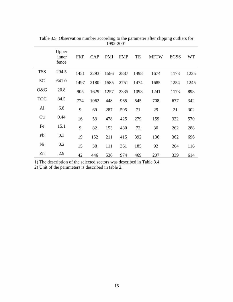
Table 3.5. Observation number according to the parameter after clipping outliers for 1992-2001
Upper inner fence
FKP CAP PMI FMP TE MFTW EGSS WT
TSS 294.5 1451 2293 1586 2887 1498 1674 1173 1235 SC 641.0 1497 2180 1585 2751 1474 1685 1254 1245
O&G 20.8 905 1629 1257 2335 1093 1241 1173 898 TOC 84.5 774 1062 448 965 545 708 677 342 Al 6.8 9 69 287 505 71 29 21 302 Cu 0.44 16 53 478 425 279 159 322 570 Fe 15.1 9 82 153 480 72 30 262 288 Pb 0.3 19 152 211 415 392 136 362 696 Ni 0.2 15 38 111 361 185 92 264 116 Zn 2.9 42 446 536 974 469 207 339 614
1) The description of the selected sectors was described in Table 3.4. 2) Unit of the parameters is described in table 2.
15

CAPEGSS
FKPFMP
MFTW PMI TE WT
DESCRIPTION
0
100
200
300
TSS
CAPEGSS
FKPFMP
MFTW PMI TE WT
DESCRIPTION
0
5
10
15
20
25
O_G
CAPEGSS
FKPFMP
MFTW PMI TE WT
DESCRIPTION
0
100
200
300
400
500
600
700
SC
CAPEGSS
FKPFMP
MFTW PMI TE WT
DESCRIPTION
0
10
20
30
40
50
60
70
80
90
TOC
Figure 3.5. Distribution of TSS, O_G (Oil and Grease), SC (Specific Conductance) and TOC for nine years
16

CAPEGSS
FKPFMP
MFTW PMI TE WT
DESCRIPTION
0
1
2
3
4
5
6
7A
L
CAPEGSS
FKPFMP
MFTW PMI TE WT
DESCRIPTION
0.0
0.1
0.2
0.3
0.4
0.5
CU
CAPEGSS
FKPFMP
MFTW PMI TE WT
DESCRIPTION
0
5
10
15
20
FE
CAPEGSS
FKPFMP
MFTW PMI TE WT
DESCRIPTION
0.0
0.1
0.2
0.3
PB
Figure 3.6. Distribution of Al, Cu, Fe, and Pb for nine years
17

CAPEGSS
FKPFMP
MFTW PMI TE WT
DESCRIPTION
0.0
0.5
1.0
1.5N
I
CAPEGSS
FKPFMP
MFTW PMI TE WT
DESCRIPTION
0
1
2
3
ZN
Figure 3.7. Distribution of Ni and Zn nine years
18

Figures 3.8 and 3.9 show the number and percentage of outliers by sector for the
conventional water quality parameters and metals. Over 20 percent of Electric, Gas, and
Sanitary services (EGSS) observations are outliers for SC and TSS. Over 20 percent of
Primary Metal Industries (PMI) observations are outliers for lead and zinc. Over 20
percent of Transportation Equipment (TE) samples are outliers for copper.
Discriminant analysis (Systat 10) was used as a preliminary classification approach to
discriminate among the eight sectors. The data cases that contain both the mandatory
conventional water quality parameters (pH, TSS, SC, TOC, Oil and Grease) and metals
are very limited. For this reason, discriminant analysis was performed only for
conventional water quality parameters. The analysis indicates which parameter is more
valuable to differentiate among the different class. Figure 3.10 shows the result of
discriminant analysis. The more useful parameters for this purpose are pH, SC, and Oil
& Grease. However, only 19 percent of the data were correctly classified. The
distribution of the eight sectors using a linear combination of the three parameters totally
overlaps.
Figure 3.11 shows an example of successful discriminant analysis. The example uses
well-known Iris flower data. The patterns allow one to recognize three types of flowers
from four parameters.
To further seek a relationship between water quality data and various activities of
industries, a supervised neural network, multi-layer perceptron model was used. Neural
Connection 2.1 (SPSS Inc. and Recognition System Inc, Chicago, IL) was used to build
the neural model. The neural model was extensively trained with various architectures.
The performance was only a little better than using the discriminant analysis (see Table
3.6). The performance was still very poor and only 15 to 31 percent of the cases were
correctly classified for each sampling season.
19

FKP
CA
P
PMI
FMP
TE
MFT
W
EGSS WT
0
100
200
300
400
500
Num
ber o
f out
liers
TSS
0
100
200
300
400
SC
0
100
200
O&
G
0
40
80
120
160
TOC
FKP
CA
P
PMI
FMP
TE
MFT
W
EGSS WT
0
10
20
30
Out
liers
(%)
TSS
0
5
10
15
20
25
SC
0
5
10
15
20
25
O&
G
0
4
8
12
16
20
TOC
Figure 3.8. Distribution of number and percentage of outliers according to its sector for
TSS, SC (Specific Conductance), O&G (Oil and Grease) and TOC
FKP
CA
P
PMI
FMP
TE TW
EGSS WT
MF
0
20
40
60
Num
ber o
f out
liers
Al
0
20
40
60
80
Cu
0
40
80
120
160
Pb
0
40
80
120
160
Zn
FKP
CA
P
PMI
FMP
TE TW
EGSS
MF W
T
0
4
8
12
16
Out
liers
(%)
Al
0
5
10
15
20
25
Cu
0
10
20
30
Pb
0
5
10
15
20
25
Zn
Figure 3.9. Distribution of number and percentage of outliers according to its sector for Al, Cu, Pb, and Zn
20

Figure 3.10 The result of the discriminant analysis
Figure 3.11 An Example of discriminant analysis using the Iris data
21

Table 3.6. Results of a neural model, multi-layer preceptron.
Season Correct classification (%)
Case number of
training file
Parameters = input variables
Categories based on SIC = output variables
92-93 30.64 235 pH, TSS, SC 20,28,33,34,37,42,49 93-94 24.57 814 pH, TSS, SC 20,28,33,34,37,42,49
18.76 1125 pH, TSS, SC 20,28,33,34,36,37,42,4994-95
28.45 840 pH, TSS, SC, Oil&Grease 20,28,33,34,36,37,42,4995-96 17.08 890 pH, TSS, SC, Oil&Grease 20,28,33,34,37,42,49
28.40 960 pH, TSS, SC 20,28,33,34,37,42,49 96-97
31.31 674 pH, TSS, SC, Oil&Grease 20,28,33,34,37,42,49 97-98 14.65 314 pH, TSS, SC, Oil&Grease 20,28,33,34,37,42,50
SIC; Standard Industrial Classification
22

The data set was also examined to determine if a seasonal first flush could be identified.
alifornia has a Mediterranean te typified by winter and spring precipitation and
summer drought. Most western parts of California including Los Ange
May to August. Figure 3.12 shows the monthl l for si
C ia duri - 2000. rds y average rainf
o ttp://w dc.noaa a/ /ccd/nrmlprc
C clima
les are dry from
x locations in y average rainfal
aliforn ng 1971 Reco of the monthl all were obtained
nline (h ww.nc .gov/o climate/online p.html). This
ra attern a long p or d-up and the fi
season usually has higher pollu on a
fl
To determine a seasonal first flush phen t
r ree yea orm wat nit T
ears are shown in Figures 3.13 through 3.15.
ow data are shown. The daily precipitation
record from Los Angles Civic Center station was used for the rainfall and antecedent dry
days instead of real site rainfall data, which is not monitored. Records of the daily
precipitation data were obtained online (http://www.nwsla.noaa.gov/climate/climate.html
infall p creates eriod f pollutant buil rst storm of the
tant c centrations, which is called “seasonal first
ush.”
omenon for GISP storm wa er discharges, the
ecent th rs of st er mo oring data were examined. SS, specific
conductance, TOC, and Zn for the three y
Since flow monitoring is not required, no fl
).
Although, rainfall will vary by site, the record from Civic Center was used as
representative of the general pattern of rainfall for Los Angeles area.
The GISP requires that the first storm and one later storm be sampled. In some cases, the
first sample does not represent the first rainfall event. Several events for each sampling
year were sampled by the GISP permittees, which means that some storm events have
more cases than other storm events. The permittees had no direct guidance for selecting
storm events other than an early event in the rainfall year.
The guidance to select the first storm of the year virtually ensures that high data will be
observed. Median concentrations of all parameters were highest in the initial event of
storm water and decreased--except during the 1998-1999 season. The four parameters
show similar trends for all events. The rainfall pattern in California is such that most
portions of the state are likely to experience a seasonal first flush. Therefore, data
collected using sampling strategies based upon first storm data can be biased high.
23

24
JAN
FEB
MAR AP
RM
AY JUN
JUL
AUG
SEP
OC
TN
OV
DEC
0
0.5
1
1.5
2
2.5
p(
)
Fresno, CA
JAN
FEB
MAR AP
RM
AY JUN
JUL
AUG
SEP
OC
TN
OV
DEC
0
1
2
3
4
5
Pre
cipi
tatio
n(in
ch)
Santa Barbara, CA
JAN
FEB
MAR AP
RM
AY JUN
JUL
AUG
SEP
OC
TN
OV
DEC
0
0.5
1
1.5
2
Prec
ipita
tion(
inch
)
2.5San Diego, CA
JAN
FEB
MAR AP
RM
AY JUN
JUL
AUG
SEP
OC
T V CN
O DE
0
0.5
1
1.5
2
2.5
3
Prec
ipita
tion(
inch
)
3.5Los Angeles, CA
JAN
FEB
MAR AP
RM
AY JUN
JUL
AUG
SEP
OC
TN
OV
DEC
0
1
2
3
4
5P
reci
pita
tion(
inch
)San Francisco, CA
JAN
FEB
MAR AP
RM
AY JUN
JUL
AUG
SEP
OC
T VN
O DEC
0
1
2
3
4
Prec
ipita
tion(
inch
)
Sacramento,CA
Figure 3.12. Monthly average rainfall in California, 1970-2000

0 0.2 0.4 0.6 0.8 1 Normalized Cumulative Precipitation,1998-1999
40
80
120
160
200S
C(u
mho
s/cm
)
8
12
16
20
24
28
32
TOC
(mg/
l)
0.3
0.4
0.5
0.6
0.7
0.8
Zn (m
g/l)
SCTOC ZnTSSRainfallAnte. dry day
0
1
2
Rai
nfal
l (in
ch)
04080
Ant
eced
net
dry
per
iod
(day
)
30
40
50
60
70
TSS
(mg/
l)
Figure 3.13. Distribution of TSS, SC (Specific Conductance), TOC and Zn for 1998-
1999
0 0.2 0.4 0.6 0.8 1 Normalized Cumulative Precipitation,1999-2000
40
80
120
160
200
240
SC
(um
hos/
cm)
0
10
20
30
40
TOC
(mg/
l)
0.2
0.4
0.6
0.8
1
1.2
Zn (m
g/l)
SCTOC ZnTSSAnte. dry dayRainfall
0123
Rai
nfal
l (in
ch)
0
80
160A
ntec
edne
t d
ry p
erio
d (d
ay)
0
20
40
60
TSS
(mg/
l)
Figure 3.14. Distribution of TSS, SC (Specific Conductance), TOC and Zn for 1999-2000
25

0 0.2 0.4 0.6 0.8 1 Normalized Cumulative Precipitation,2000-2001
40
80
120
160
200
SC
(um
hos/
cm)
5
10
15
20
25
30
TOC
(mg/
l)
0.2
0.4
0.6
0.8
1
Zn (m
g/l)
SCTOC ZnTSSRainfallAnte. dry day
024
Rai
nfal
l (in
ch)
0
80
160
Ant
eced
net
dry
per
iod
(day
)
20
40
60
80TS
S (m
g/l)
Figure 3.15. Distribution of TSS, SC (Specific Conductance), TOC and Zn for 2000-
2001
26
3.3 Summary of Existing Data
The existing data show very limited utility. The variability among reported results is so
great that differences amongst different industries and landuses are not possible to
identify. Although quantitative evidence for differences in storm water runoff from
different SIC codes has not yet been documented in the published literature, it is
reasonable to assume that in most cases there should be differences. Differences in storm
water quality from different landuses have been well documented for more than 20 years
(Stenstrom, et al., 1984, Fam et al., 1987) and have become an important tool for
prioritizing BMPs. Therefore, the failure to identify quantitative differences in pollution
based on SIC codes is considered a monitoring program failure rather than the inference
that there are no differences in storm water pollutant emissions. The power of the
database provided by the monitoring program simply too weak to show the differences
at are of concern for regulators and storm water program managers.
o illustrate this effect, Table 3.7 shows the basic statistics from three GISP programs
os Angeles County, Sacramento County, and Connecticut State). The data are all
mped together for all SIC codes. The table illustrates differences among programs (e.g.,
cilities in the County of Los Angeles have a greater number of observations by far), but
e purpose of the table is to show the coefficients of variation (CV). The coefficient of
ariation is the standard deviation of the data divided by the mean of the data. Since both
atistics are in the same units, the ratio is dimensionless, which allows the variability of
ata with different magnitudes to be directly compared. The CVs in Table 3.7 range from
.17 to 16.5. This shows that in most cases the variability in the data is greater than the
ean value of the data.
his high variability may be surprising to professionals who have been monitoring water
nd wastewater treatment plant influents and effluents. Figure 3.16 shows CVs for a
pical, large west coast wastewater treatment plant influent, a large typical west coast
variability in storm water quality is drama
is
th
T
(L
lu
fa
th
v
st
d
0
m
T
a
ty
water treatment plant, and the two storm water programs being evaluated. The greater
tic.
27
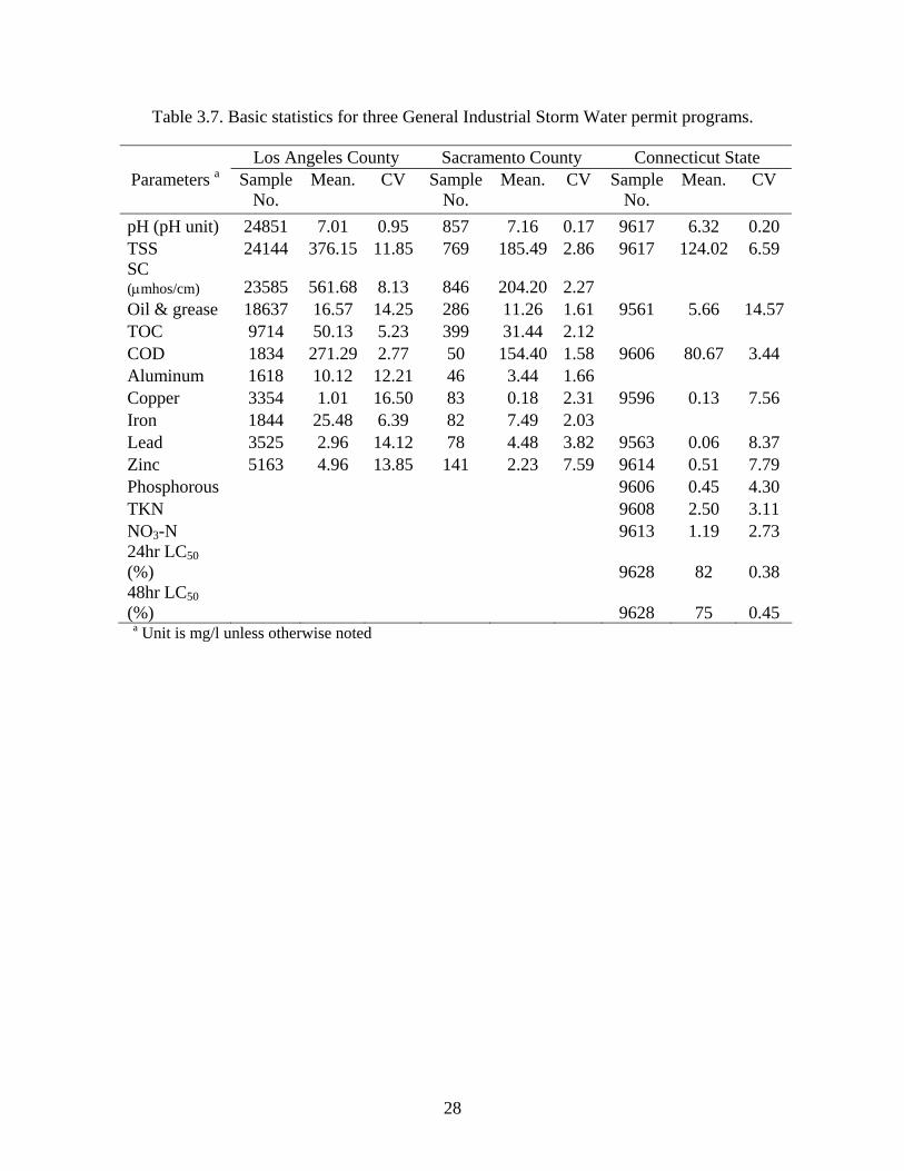
Table 3.7. Basic statistics for three General Industrial Storm Water permit programs.
Sacramento County Connecticut State Los Angeles CountyParameters a Sample
No. Mean. CV Sample
No. Mean. CV Sample
No. Mean. CV
pH (pH unit) 24851 7.01 0.95 857 7.16 0.17 9617 6.32 0.20 T 6.59
7 3.44 Alum
6
8.37 7.79
8 2.50 3.11
NO3-N 9613 1.19 2.73
(%)
SS 24144 376.15 11.85 769 185.49 2.86 9617 124.02SC (µmhos/cm) 23585 561.68 8.13 846 204.20 2.27 Oil & grease 18637 16.57 14.25 286 11.26 1.61 9561 5.66 14.57TOC 9714 50.13 5.23 399 31.44 2.12 COD 1834 271.29 2.77 50 154.40 1.58 9606 80.6
inum 1618 10.12 12.21 46 3.44 1.66 Copper 3354 1.01 16.50 83 0.18 2.31 9596 0.13 7.5Iron 1844 25.48 6.39 82 7.49 2.03 Lead 3525 2.96 14.12 78 4.48 3.82 9563 0.06 Zinc 5163 4.96 13.85 141 2.23 7.59 9614 0.51 Phosphorous 9606 0.45 4.30TKN 960
24hr LC50 (%) 9628 82 0.38 48hr LC50
9628 75 0.45 a Unit is mg/l unless otherwise noted
28

0
4
8
16
12TS BO CO NH nit
O U
S D 3
Alk
ali T
C VB
rom
i TSS
Con
duct
ivi
CO
DTK
N Cu
TSS
Con
duct
ivity
TOC
CO
DD y de ty Zn Zn
Coe
ffici
ent o
f Var
iatio
nWaste Water plantRaw WaterMunici erm atipal P it (N onal)Industrial GP ( nLos A geles)
Add
Add
Figure 3.16 Typical variability of water and wastewater treatment plant influents as compared to variability in storm water quality.
29

To illustrate the impact of the greater variability on hypothesis testing, Figure 3.17 is
provided. Each line on Figure 3.17 shows the required number of cases or observations
to conclude with 95% confidence that there is a significant difference in two means. The
assumptions are for two-tailed normal distributions. Each line represents a different CV.
The horizontal axis shows the desired difference in the means. For example, if one
wanted to detect a 50% difference in the mean pollutant discharge from two sources (e.g.,
categories or facilities, etc.), only 12 observations are required if the CV is 0.4, which
according to Figure 3.16 is typical for water and wastewaters. For storm waters, however,
the CVs are often 6 or more. For this high a CV, 2,270 observations are required. This
graph shows very dramatically that it is impractical to interpret and perform hypothesis
testing with such data. Table 3.5 shows that few categories had this many observations--
even if all nine years of the monitoring program were used. If the storm water monitoring
program is to be successful in detecting differences among permittees and categories, a
different type of monitoring with lower variability must be developed.
The use of composite samplers and professionally trained monitoring personnel is one
candidate solution to the monitoring problem. Many monitoring programs use composite
or flow-weighted composite samplers. Figure 3.18 shows data collected in such a
program. Four metals--copper, zinc, iron and nickel--are shown. Figure 3.19 shows data
from the industrial monitoring program using grab samples and untrained sampling
personnel. The difference in variabilities is dramatic and log scales are required to show
e ranges. th
30

31
0 20 40 60 80 100
1
10
100
1000
10000
100000N
umbe
r of C
ases
per
gro
up
253
64
29
1712
97 6
5
570
143
64
3724
1713
10
C.V. = 6.0
97
C.V. = 4.0C.V.= 2.0C.V.= 1.0C.V.= 0.8C.V.= 0.6C.V.= 0.4
1580
394
176
100
6445
3426
2117
6300
1580
700
394
253176
130100
7964
25117
6300
2800
1580
1010700
520394
312253
56512
14128
6300
3540
22701580
1160890
700570
4
AA
Figure 3.17. Number of observations (cases required to detect differences in means with
different variability.
Percent difference in means

Commercial
H-D-Resident
Industrial
Transportat
iVaca
nt
LANDUSE
0
50
100
150
200T_
CU
Commercial
H-D-Resident
Industrial
Transportat
iVaca
nt
LANDUSE
0
500
1000
1500
T_ZN
Commercial
H-D-Resident
Industrial
Transportat
iVaca
nt
LANDUSE
0
1000
2000
3000
4000
5000
T_FE
Commercial
H-D-Resident
Industrial
Transportat
iVaca
nt
LANDUSE
0
20
30
_NI
T
10
Figure 3.18. Distribution of Cu, Zn, Fe, and Ni in various landuse. Data are from the
landuse monitoring by LACDPW. Unit of the parameters are ug/l.
32

igure3.19 Comparison of grab samples from the General Industrial Storm Water Permit data for 1992-1998 to flow-weighted compos e samples from the industrial landuse mcomposite s
Comparison of grab sample and composite sample
TSS_GTSS_C
SC_GSC_C
TOC_GTOC_C
Trial
0.01
0.10
1.00
10.00
100.00
1000.00
10000.00
100000.00
Con
cen t
ratio
n (m
g/l o
r um
hos/
cm)
Comparison of grab sample and composite sample
CU_GCU_C
NI_GNI_C
ZN_GZN_C
Trial
0.001
0.010
0.100
1.000
10.000
100.000
1000.000
Con
cent
ratio
n (m
g/l )
Fit
onitoring data by LACDPW for 1996-2001. G indicates a grab sample and C indicates ample.
33

4. REVIEW COMMITTEE AND RECOMMENDATIONS
idway through the project, a review committee was assembled. The objective of the
view was to provide expert guidance, as well as provide stakeholder insight. The
llowing individuals attended a meeting on the UCLA campus on November 17, 2003.
heir agency or employer is shown.
Name Agency or Employer
Michael Drennan Brown and Caldwell (consulting firm) Mark Gold Heal-the Bay (NGO) Gerry Green City of Downey Kosta Kaporis City of Los Angeles, Bureau of Sanitation Ken Schiff Southern California Coastal Water Research Project (Joint
Powers Agency monitoring coastal waters) Eric Strecker Geosyntec, Inc (consulting firm) Xavier Swamikannu California Regional Water Quality Control Board,
Los Angeles Region Tracy Wilcox MWH, Inc (consulting Firm) Surfrider Foundation (NGO)
ost of the material contained in Section 3 was presented at the meeting and the
llowing suggestions were made as desirable or necessary inclusions in a new permit:
1. The new permit should clearly state its objectives. Three objectives are
recommended: being able to identify high emitters (polluters); encouraging
pollution prevention; and creating data for use by planners and particularly by
developers of TMDLs.
2. The monitoring program should have more specifications. Among those
recommended are requirements for the use of certified laboratories, except for
field measurements; trained sampling personnel; quality assurance plans;
improved sampling protocols; and specification of analytical techniques,
including minimum detection limits.
ude
M
re
fo
T
M
fo
3. Expand the list of monitored pollutants to include industry-specific pollutants
(e.g., metals analysis for those industries likely to be discharging metals). Incl
parameters in the Clean Water Act Section 303(d) listing for industries in
34

impacted watersheds. Allow requirements for monitoring specific pollutants to
expire if they are routinely not detected.
ll
t of the permit. An example is estimating the
ct runoff. In this way, a
eviewing the data collected by the permittees will be able to estimate
m f
5. i g resu e to regulators. A web-based
to eliminate
e ors by
sea water, neither of
o be
ble by authorized personnel
gram should be able to
was done and was included in Figures 3.17 in the previous Section. The group
partially
7. ew
irements are being implemented, the permittees should
. The
ld
od
from
4. The committee was reluctant to require flow weighted composite sampling of a
permittees. Only the larger permittees should be required to perform such
sampling. For smaller permittees, a method of estimating flow should be
developed and included as par
amount of impervious area and other factors that affe
person r
mass emissions fro low rate and concentrations.
Make monitor n lts available in real-tim
reporting method was proposed. Such a procedure should be able
transcription rr ic conductivity flagging implausible values (e.g., the specif
data shown earlier ranges from the best distilled water to
which is likely for sto monitoring program should alsrm water runoff). The
able to include the data into a database that is accessi
so that routine reports can be generated. In addition, the pro
identify problematic data for early investigation.
6. Answer the question, “How much more data is required to make decision?” This
was interested to know if simply collecting more samples would solve or
solve the problem or if better protocols are also required.
The new permit will likely increase cost and training requirements. While the n
monitoring program requ
be exempt from monitoring (anticipated to be 12 to 24 months maximum)
State Board should develop a new guidance and training document, which shou
include training material on the new requirements. A method to select a go
sampling site and estimating flow rate are two new topics that will benefit
guidance and training.
35

The gro
that the h emitters (polluters) and should be web
bas
up felt that from all of the recommendations made, the two most important were
new permit should be able to identify hig
ed to speed up reporting and eliminate implausible values.
36

5. PROPOSED REQUIREMENTS OF THE NEW MONITORING PROGRAM.
New provisions are proposed for the new monitoring program. These are based in large
part on the recommendations of the review committee, as well as in part of the experience
of the research team and their findings in the project. They are divided into three general
sections: sampling methodology, parameter selection, and reporting method. There are
also recommendations for future research and development that will improve monitoring
techniques.
5.1 Sampling Methodology
The sampling methodology is probably the most lacking part of the existing permit. The
new permit should require a minimum level of training for sampling personnel for all but
the smallest of facilities. Training is required to ensure that representative sites are chosen.
The skills to do this are beyond most industrial employees who have had no reason to be
trained in this area before. Alternatively, a certified laboratory or professional engineer
can be employed.
Certified laboratories or consultants may offer the best opportunity to implement the new
training program. Certified laboratories and consultants are already familiar with many
sampling issues since they may be sampling or monitoring results in other environmental
sampling programs. Typical issues, such as sampling preservation and holding time
should be well known to them.
A model is envisioned for a certified laboratory to perform the sampling, which will
involve the permittee, as well as laboratory personnel. Laboratory personnel can
complete a training program provided by the State Board where they receive instruction
on the monitoring program requirements, as well as general knowledge of representative
sampling techniques. The permittee contracts with a laboratory for sample analysis, and
in so doing, is contracting with the laboratory to set up a representative sampling program.
In this way, the certified laboratory provides a “package”--a sampling plan, analytical
services and reporting.
37

A model exists for permittees to use consultants for monitoring. The California
Department of Transportation (Caltrans) was required to monitor freeway runoff in many
areas of the state. They successfully contracted with consultants to perform the
monitoring, quality assurance, and reporting. The State Board may wish to adopt a
similar approach utilizing monitoring funds paid by industrial permittees to perform
targeted samplings. Through this process, a subset of representative sites could be
selected, which w
ill result in financial savings to the permittees.
o storms per season--maybe adequate, but more guidance
is needed. For example, collecting the first runoff of an early storm creates a bias. The
t
were selected for convenience, low cost, and ability to measure in
e field. Their environmental significance is sometimes limited. For example, the
t
e measured reliably and accurately. The following list of
ut
The frequency of sampling--tw
sampling plan should provide some way of compositing samples. Even if only several
grab samples are composited, this will be an improvement.
5.2 Parameter Selection
The rationale for choosing the existing parameters is not known to the research team, bu
it appears that some
th
specific conductivity is of little importance in predicting the environmental impact of
storm water on receiving waters. Only the most pristine of receiving waters will have
conductivities lower than most storm water. The value of the conductivity measurements
is counter-intuitive. It has shown that an easily measured parameter using reliable, bu
inexpensive instruments cannot b
parameters is proposed:
Some of the measurements are included because of environmental significance, b
others are included because they are either simple, inexpensive, and/or are useful in
determining the reliability of the monitoring program. The specific conductivity analysis
is retained because it can serve as a validity check and because is it very inexpensive to
perform. Oil and Grease has been omitted for two reasons: it is not a trivial test and
requires care in sampling since oil adsorption to glassware and sampling equipment can
38

be significant. The environmental significance of Oil and Grease, as well as efficiency of
t al.,
Turbidity
ptional measurements
ther regulator needs to be able to add specific parameters
e
arge
y to detect small differences, and as shown earlier, was one of
e more useful parameters.
ing a
the measuring technique depends upon the source (Stenstrom et al., 1986, Fam, e
1987). In addition, Oil and Grease from highway runoff, COD or TOC are adequate
surrogates (Khan, et al., 2004).
The following minimum list of parameters is proposed:
Field measurements Specific Conductivity pH Laboratory measurements
Total suspended solids Chemical oxygen demand or total organic carbon
Total metals – cadmium, chrome, copper, lead, nickel, zinc O
The Regional Board or ano
when they may be needed. This would include parameters on the Clean Water Act
Section 303(d) impacted waters list. Nutrients, such as nitrogen and phosphorous are th
likely candidates. In addition, pesticides from industries that are likely to be using l
amounts of pesticides in their business or industries whose runoff discharges into
sensitive surface waters are also good candidates. These measurements will be made in
the field or in a laboratory as required.
Toxicity is also a good candidate for additional measurements. While toxicity is quite
expensive, it has the abilit
th
5.3 Reporting Method
One of the most significant improvements that can be made to the existing monitoring
program is to require web based reporting. Although it will require the State Board to
develop a program and maintain servers, this effort should be less costly than manag
paper based reporting system.
39

The web-based reporting has several important advantages. First, it provides data to th
regulatory agencies in real-time. The server can be programmed to provide periodic
summary reports. Second, permittee
e
s will most likely find it easier to use web based
he web based reporting.
has another advantage that may not be obvious. The parameters
e values. The range of specific conductivity for storm
n and ranges outside this value are probably errors. Many are
scription errors--the wrong units are used or a person’s
handwriting is hard to read. A web based reporting system can incorporate a simple
usly implausible or unlikely value of pH is reported (e.g., 11 or
s or
g water monitoring requirements. The MS4 permittees are
quired to operate or contract with state certified laboratories. The MS4 permittees are
erform the industrial monitoring required by the existing permit
Ls.
reporting. If certified laboratories are used, they can do t
Web based reporting
being reported all have plausibl
water is reasonably know
obviously reporting or tran
expert system that can query the user.
For example, if an obvio
higher), the person entering the data can be asked to confirm the entry. If it is still
implausible, the person can be asked a second question, such as confirming the unit
the person can suspend the reporting and come back after checking the data. Finally, if no
error is found, the program accepts the implausible data and marks it for attention by the
appropriate person at the regulatory agency. The web based system can also be
programmed to create summary or annual reports.
5.4 Co-Sampling Programs
There are many Municipal Separate Storm Sewer System (MS4) permittees in the State,
and they are required to develop and implement municipal storm water monitoring
programs that include receivin
re
trained and equipped to p
and the new proposed permit. The MS4 permittees are also charged with meeting TMD
40

The TMDL requirement provides an incentive for MS4 permittees to locate discharges
ill
option
as
or laboratories.
that are causing water quality violations. Therefore, they have an incentive to locate and
correct high emitters.
An alternative that should be available, is for industrial permittees to fund the MS4
permittees to do the required monitoring and reporting. The economies of scale w
ensure that the cost of funding MS4 programs will be less than the industrial permittees
would have to pay to do the work themselves. The MS4 permittees would have the
responsibility for selecting the number of industrial permittees to be sampled and through
this process, attempt to locate and correct high emitters. This could be a desirable
for small facilities and might help MS4 permittees more easily meet TMDLs, as well
provide funding to support technicians
41

6. CONCLUSIONS
Data collected from the California statewide General Industrial Storm Water Permit
(GISP) was examined over the nine-year period from 1992 to 2001. The data were
and
der
2. There are several sources for the variability and the use of grab samples,
untrained sampling personnel, and a limited selection of monitored parameters are
among the largest sources.
3. The data generally do not allow for hypothesis testing and generally could not be
used to identify high dischargers using statistical tests with confidences of 0.05 or
greater. The data also could not be used to identify differences in discharges from
different types of industries.
4. The variability in the collected data is so great that the collection of additional
data points, up from two to ten or more storms per year, will still not provide the
needed precision. Improving the precision of sampling, by using composite
samples for example, is a more promising approach.
5. The data collected in Los Angeles has greater means, medians, and variability
than data collected by two similar programs (Sacramento, CA and the state of
Connecticut). The frequency of exceeding US EPA target levels is also greater for
the Los Angeles data.
6. A review committee composed of experts from consulting, government, and
NGOs suggested improvements for a new permit. Among the most important of
those were requirements for trained sampling personnel, certified laboratories,
evaluated to determine if it could be used to identify permittees with high emissions
if the storm water loads from various classes of industries could be characterized in or
to create rankings and typical emission rates. The data were also compared to data
collected in other monitoring programs. The following conclusions are made:
1. The data collected by the permittees are highly variable with coefficients of
variation as high as 16.5. This compares to coefficients of variation, generally
less than 0.5 for other environmental monitoring programs, such as water and
wastewater treatment plant influents.
42

and web-based reporting. The most important goal for the new permit is to be able
ned
to identify high dischargers.
The requirements of a new monitoring program are proposed. They include a broade
suite of parameters, use of composite samples and certified laboratories, joint sampling
programs, and a web-based reporting system. It is also proposed that the current
monitoring program be suspended while the State Board develops the new program.
43

7. REF
ay, S., Jones, B.H., Schiff, K. and Washburn, L. (2003) Water quality impacts of
, 997-
ff from metal plating facilities, Los Angeles, California. Waste Management, 18, 25-38.
am, S,. Stenstrom, M.K. and G. Silverman, G (1987) “Hydrocarbons in Urban Runoff,” Journal of the Environmental Engineering Division, ASCE, Vol. 113, pp 1032-1046.
Khan, S., Lau, S-L, Kayhanian, M. and Stenstrom, M.K. (2004) Oil and Grease Measurement in Highway Runoff – Sampling Time and Event Mean Concentrations. submitted to the Journal of Environmental Engineering, ASCE.
Lee, H. and Stenstrom, M.K. (2005) Utility of stormwater monitoring. Water Environmental Research, Vol. 77, No. 1.
Lee, H., Lau, S-L., Kayhanian, M. and Stenstrom, M.K. (2004) Seasonal first flush phenomenon of urban stormwater discharges. Water Research, 38, 4153-4163.
Lee, J.H., Bang, K.W., Ketchum, L.H., Choe, J.S., and Yu, M.J. (2002) First flush analysis of urban storm runoff. The Science of the Total Environment, 293,163-175.
Leecaster, M.K., Schiff, K. and Tiefenthaler, L.L. (2002) Assessment of efficient sampling designs for urban stormwater monitoring. Water Research, 36, 1556-1564.
Ma, J-S., Khan, S., Li, Y-X., Kim, L-H., Ha, H., Lau, S-L., Kayhanian, M., and Stenstrom, M.K. (2002) Implication of oil and Grease measurement in stormwater management systems. Presented at the 9th ICUD, Portland, Oregon, September 2002.
Pitt, R., Maestre, A. and Morquecho, R. (2003) Compilation and review of nationwide MS4 stormwater quality data. Proceedings of 76th Water Environment Federation Technical Exposition and Conference, Los Angeles, CA, 2003.
Pitt, R (2004) http://unix.eng.ua.edu/~rpitt/Research/ms4/Final%20Table%20NSQD%20v1_1%
ERENCES
Bstormwater discharges to Santa Monica Bay. Marine Environmental Research, 56, 205-223.
Davis, A.P., Shokouhian M. and Ni, S. (2001) Loading estimates of lead, copper, cadmium, and zinc in urban runoff from specific sources. Chemosphere, 441009.
Duke, L.D., Buffleben, M. and Bauersachs, L.A. (1998) Pollutants in storm water runo
F
20020704.xls . Sansalone, J.J. and Buchberger, S.G. (1997) Partitioning and first flush of metals in urban
roadway storm water. Journal of Environmental Engineering, ASCE, 123(2), 134-143.
Stenstrom, M. K., Silverman, G.S. and Bursztynsky, T.A., (February 1984) Oil and Grease in Urban Stormwaters, Journal of the Environmental Engineering Division, ASCE, Vol. 110, No. 1, pp 58-72.
44

Stenstrom, M.K., Fam S., and Silverman (1986), G.S.Analytical Methods for Quantitative and Qualitative Determination of Hydrocarbons and Oil and Grease in Wastewater, Environmental Technology Letters, Vol. 7, pp 625-636.
Stenstro to Santa Monica Bay. Vol. I, Annual Pollutants Loadings to Santa
. I, pp
Stenstro ., Lau, S-L., Lee, H-H., Ma, J-S., Ha, H., Kim, L-H., Khan, S. and
Stenstro ., Lau, S-L., Ma, J-S., Ha, H., Lim, L-H., Lee, S., Khan, S. and
Stenstr K., Lau, S-L., Lee, H-H., Ma, J-S., Ha, H., Kim, L-H., Khan, S. and r3).
02. Stenstro
ear4). nia Transportation, July, 2003.
m, M.K. and Strecker, E. (1993) Assessment of Storm Drain Sources of ContaminantsMonica Bay from Stormwater Runoff, UCLA-ENG-93-62, May 1993, Vol1-248. m, M.K
Kayhanian, M. (2000) First Flush Stormwater runoff from Highways. Research report for California Department of Transportation, September, 2000. m, M.K
Kayhanian, M. (2001) First Flush Stormwater runoff from Highways. Research report for Department of California Transportation, September, 2001. om, M.Kayhanian, M. (2002) First Flush Stormwater runoff from Highways (yeaResearch report for Department of California Transportation, July, 20m, M.K., Lau, S-L., Lee, H-H., Ma, J-S., Ha, H., Kim, L-H., Khan, S. and
Kayhanian, M. (2003) First Flush Stormwater runoff from Highways (yResearch report for Department of Califor
45

APPENDIX
Design of Storm Water Monitoring Programs for Industrial Sites:
A Manuscript Submitted to Water Research
Haejin Lee and Michael K. Stenstrom

Design of Storm Water Monitoring Programs for
Industrial Sites
Haejin Leea, Seung-jai Kimb and Michael K. Stenstromc*
a United States Department of Agriculture, Natural Resources Conservation Service,
El Centro Office, 177 N. Imperial Ave., El Centro, California 92243, USA
bDepartment of Environmental Engineering, Chonnam National University,
300 Yongbong-dong, Buk-gu, Gwangju 500-757, KOREA
c Department of Civil and Environmental Engineering, 5714 Boelter Hall, University of
California, Los Angeles, Los Angeles, California 90095, USA
Abstract Storm water runoff is now the leading source of water pollution in the United States, and
storm water monitoring programs have only recently been developed. This paper
evaluates more than 20 storm water monitoring programs and datasets to determine their
usefulness in characterizing discharges and achieving their ultimate goal of reducing
storm water pollution. The monitoring results are highly variable, with coefficients of
variation that are 2 to 60 times higher than those observed in water or wastewater
monitoring programs. Although the monitoring programs could not differentiate metals
contribution from different types of industries, industrial land use is an important source
of metals. Data from California, which has distinct dry periods, showed a seasonal first
flush, whereas data from Connecticut did not show a seasonal first flush.
47

Recommendations for improving monitoring programs include using composite samplers,
selecting alternate or additional water quality parameters, alternate timing of sample
collection, and strategies that sample a subset of the total permittees using more
sophisticated methods.
Keywords: First flush; Industrial General Permit; Monitoring; Municipal Permit; Storm water
1. Introduction
The completion of wastewater treatment plants mandated by the Clean Water Act has
reduced pollution from point sources to the waters of the United States. As a result, non-
point sources pollution such as storm water runoff are now the major contributor to
pollution of receiving waters. The problem of storm water pollution is growing worse
because of continuing development, which results in increased impervious surface area.
In order to reduce storm water pollution, regulatory agencies are requiring storm water
monitoring programs. The programs are implemented through the National Pollutant
Discharge Elimination System (NPDES) Storm water Permit.
Although the overall goal of storm water monitoring programs include the identification
of high risk dischargers, it is also for the development of a better understanding of the
mechanisms and sources of storm water pollution with the long-term goal of reducing
pollutants to less harmful levels. Most storm water monitoring programs are relatively
new and evaluations of their usefulness for satisfying these goals are only now possible
(Duke et al., 1998; Lee and Stenstrom, 2003; Pitt et al., 2003). In 2003, Lee and
evaluated the General Industrial Storm Water and Municipal Storm Water Permits for
Los Angeles County for three wet seasons (1998 - 2001) and five wet seasons (1996 -
2001), respectively. The results of our previous study suggest that parts of the current
48

industrial storm water monitoring programs will not be helpful to identify high
dischargers, nor will they be useful in developing Total Maximum Daily Loads
(TMDLs). The design and requirements of the monitoring programs do not produce data
with sufficient precision for decision-making.
In this paper, we evaluated a number of storm water monitoring programs to determine
their usefulness in achieving their dual goals, as well as make recommendations for
improvement. Our analysis included more than 20 monitoring programs and datasets,
which covered three General Industrial Storm water Permit programs--US EPA’s Multi-
Sector Storm Water General permit (MSGP) program, Municipal Storm Water Permit
programs from 17 states, and Caltrans’ first flush highway runoff characterization study.
The programs are summarized in Table 1. We believe our results will be helpful to
planners and regulators to interpret existing datasets and programs, as well as provide
recommendations for improving the future programs.
2. Background
2.1. General Industrial Storm Water Permit Programs
The General Storm Water Industrial Permit (GISP) Programs require facilities that
discharge storm water associated with the industrial activities directly or indirectly to
apply and obtain coverage under the GISP. Industries are categorized by Standard
Industrial Classification (SIC) codes. Industrial monitoring programs generally vary by
state. Currently, there are approximately 3,000 permittees within Los Angeles County.
Under the monitoring requirements, permittees must collect water quality samples from
two storms per year and analyze four conventional parameters: pH, specific conductance
49

(SC), total suspended soils (TSS), and oil and grease (O&G). Total organic carbon (TOC)
can be substituted for oil and grease, and certain facilities must analyze for specific
additional pollutants such as metals. Permittees are requested to collect storm water
samples during the first hour of discharge from the first storm event of the wet season and
at least one other storm event later in the wet season. In our previous study (Lee and
Stenstrom, 2003), we analyzed data from three recent wet seasons (1998-2001) . In this
study, we extended the evaluations to the available data, which covered a total of nine
wet seasons (1992-2001), and we also analyzed eight wet seasons (1993-2001) of data
from a similar GISP in Sacramento County.
Nine years (1995-2003) of storm water data were available from the State of Connecticut.
Their program requirements are different from California’s requirements. Permittees in
Connecticut must analyze for three metals (total copper, lead, and zinc), nutrients (total
phosphorous, total Kjeldahl nitrogen and nitrate as nitrogen), aquatic toxicity (LC50), and
conventional parameters (pH, COD, O&G and TSS). They must collect a grab sample
within the first 30 minutes of runoff from at least one storm per year.
The U.S. Environmental Protection Agency (USEPA) issued the Multi-Sector Storm
Water General permit (MSGP) for storm water discharges associated with most industrial
activities in September 1995 (revised in 2000). The permit covers industrial activities in
states and territories that have not been authorized to run the NPDES general permitting
program. The types of monitoring and required parameters vary among industry sectors
and sub-sectors. Grab samples may be used except at airports, which must collect a flow-
weighted composite in addition to a grab sample. Grab samples are to be collected within
50

the first 30 minutes of discharge. Permittees are required to sample every other year. Six
years (1998-2003) of data were available.
2.2. Municipal Storm Water Permit Programs
The Storm Water Program for Municipal Separate Storm Sewer Systems (MS4) is
designed to monitor and reduce sediment and pollution that enters surface and ground
waters from storm sewer systems to the maximum extent practicable. Storm water
discharges associated with MS4s are regulated using NPDES permits. Under US EPA
sponsorship, Pitt et al (2003) compiled and evaluated storm water data from a
representative number of NPDES MS4 storm water permitees. Over ten years of data
from more than 200 municipalities throughout the United States were assembled. The
areas were primarily located in the southern, Atlantic, central and western parts of the
United States. Only data from well-described storm water outfall locations were used in
the database. Most pollutants were characterized using flow-weighted composite
samples except for pollutants having restrictive holding time requirements, such as
bacterial indicators, which were sampled using grab samples. Numerous pollutants were
analyzed including typical conventional pollutants, heavy metals, and organic toxicants.
Los Angeles County MS4 data were not included in the database.
Since the 1970’s, the Los Angeles County Department of Public Works (LACDPW) has
had its own municipal monitoring program. In 1994, they began an improved program,
which was designed to determine total pollutant emissions to coastal waters, as well as
landuse specific discharges (Stenstrom and Strecker, 1993). Total emissions are
estimated from flow-weighted composite samples that are collected at five sampling
51

stations (four stations are required under the 1996 NPDES Municipal Permit and one
station remains from an earlier permit.). The stations are equipped with flow monitoring
equipment and operate unattended in secure facilities. Many water quality parameters are
measured, including indicator organisms, general minerals, nutrients, metals, semi-
volatile organic compounds, and pesticides.
2.3. Caltrans First Flush Monitoring Study
The Department of Civil and Environmental Engineering at UCLA has characterized
storm water runoff from three highway sites for California Department of Transportation
(Caltrans) since 1999 (Stenstrom et al., 2000, 2001, 2002, and 2003). The study was
conducted to assess runoff water quality and quantity from California freeways with
particular emphasis on characterizing runoff during the early stage of storm events. Grab
samples were collected every 15 minutes during the first hour of the storm. After the first
hour, additional grab samples were collected each hour for up to 8 hours. An automatic
composite sampler was also used after the first year to collect flow-weighted composite
samples. A large suite of constituents including indicator bacteria, general minerals,
nutrients, oil and grease, organic, and metals were monitored.
52

3. Utility of the programs
3.1. Variation
Our early results showed that storm water data sets are fundamentally different that data
sets derived from water and wastewater monitoring programs. The variability of storm
water data--especially industrial storm water data--is much greater than commonly found
in potable water or wastewater datasets. This results in part because of the time-varying
nature of storms, but is also due to the use of grab samples and less experienced
monitoring personnel. Most of the storm water monitoring programs allow for self-
monitoring, which is similar to water and wastewater programs. The important
difference is that many storm water permittees usually have no experience with water
quality monitoring, whereas the water and wastewater permittees are usually formally
trained and certified in the operation of a water or wastewater plant.
Figure 1 illustrates this difference in monitoring programs and shows the coefficient of
variation (CV) for various routinely monitored water quality parameters. The leftmost
bars show the CVs for influent wastewater quality parameters, which are typical for large
west coast wastewater treatment plants. The CVs range from 0.09 to 0.2. The next set of
bars show the CVs for raw water quality parameters for a large Los Angeles area potable
water treatment plant. The CVs range from 0.07 to 0.3. The next group of bars shows the
CVs from the Municipal Storm Water Permit which range from 1.1 to 3.3 (Pitt 2004).
The final group of bars shows the CVs from the GISP data for Los Angeles County. The
CVs range from 2.8 to 14.
53

This graph dramatically illustrates the difficulty in using storm water monitoring data.
The variability in the data is several times the mean value. With such high variability, it is
virtually impossible to make statistical inferences, even for such simple matters as
identifying high dischargers. The sampling method is a major source of much of the
variation. For GISP monitoring, grab samples are allowed, whereas flow-weighted
composite samples were collected in the Municipal Storm Water Permit program. Water
and wastewater treatment plant data are generally collected with composite samplers.
Reducing the variability in data collection is the first problem that needs to be solved to
improve the current monitoring program. In the recommendation section, we discuss the
problem in detail and suggest ways to reduce the variability for improving future
programs.
3.2. Regional Differences
Figure 2 shows the percentage of the data collected under the GISP and Multi-sector
General Permit (MSGP) that falls outside the US EPA’s benchmarks. Only the data from
Massachusetts are shown for the MSGP, which had the largest number of observations;
most other states had too few data to analyze. Data from Los Angeles County have the
highest percentage outside the benchmark for all parameters except pH. Zinc exceeds the
benchmark level in over 50 percent of samples for all of the monitoring results and in
over 90 percent of the observations from Los Angeles County. The data from Except for
pH, Connecticut has the lowest percentage outside benchmark. Table 2 shows the basic
statistics for the three major industrial monitoring. In general, samples from Los Angeles
have the highest mean concentration and the largest range of CV for all parameters
among the three GISP programs.
54

Climatic conditions, such as the existence of long dry periods may greatly impact
pollutant emissions from urban storm water discharges. Figure 3 shows the monthly
average rainfall for Los Angeles, California and Hartford, Connecticut during 1971-2000
(http://www.ncdc.noaa.gov/oa/climate/online/ccd/nrmlprcp.html). Most western parts of
California, including Los Angeles and Sacramento are dry from May through September.
This rainfall pattern creates a long period for pollutant build-up and, therefore, the initial
storm of the wet season may have higher pollutant concentrations than in later events
(Lee et al., 2004). This phenomenon is called a “Seasonal First Flush,” and is illustrated
in Figure 4. Figure 4 shows the median concentrations of Specific Conductance, TOC,
TSS, and Zn as a function of the normalized cumulative precipitation during the 2000-
2001 wet season for GISP data from Los Angeles County. The first event of the wet
season clearly has greater pollutant concentrations, and if only the first storm is
monitored, it will overestimate pollutant concentrations in later storms. Areas with more
uniform rainfall, such as Connecticut did not shown a seasonal first flush. This presence
of a seasonal first flush is a dilemma for monitoring programs, which attempt to identify
high dischargers, as well as estimate central tendencies, such as yearly emissions.
3.3. Facility Landuse Differences
In our previous study (Lee and Stenstrom, 2005), we used several statistical procedures
and several types of neural networks to identify relationships between water quality data
and various landuses for three wet seasons (1998-2001). In this study, we extended the
analysis to the previous six wet seasons (1992-1998) and we also analyzed eight wet
seasons (1993-2001) of Sacramento County’s data and the nine years (1995-2003) of
55

Connecticut’s data. Eight major industries were selected--food and kindred products;
chemical and allied products; primary metal industries; fabricated metal products;
transportation equipment; motor freight transportation and warehousing; electric; gas;
sanitary services; and whole trade-durable goods. Outliers in the data set were first
eliminated and were defined as greater than 1.5 times the interquartile range plus the 75%
data or less than 25% data minus 1.5 times the interquartile range. The lower value was
generally zero. The neural models were extensively trained using various architectures;
however, as previously observed, the performance of all models was very poor
confirming that no relationship exists between the industrial categories based on SIC
code and the storm water runoff quality.
To further evaluate relationships between water quality and various types of industries, a
t-test for two industrial categories was used. The food and kindred products and primary
metal industry were selected for demonstration because they are both major industries
with many observations and representative industry for a light and heavy industry,
respectively. In addition, the nature of the businesses suggests that there should be
differences in storm water runoff quality. Data from two GISP programs, Los Angeles
County and Connecticut were analyzed.
Table 3 shows the case number and basic statistics for the two categories from the two
regions after removal of outliers. The mean concentrations for all parameters are
dramatically reduced as compared to the original data (Table 2). The table shows the t-
value and the associated probability of obtaining a false result (Type I error) from a two-
group t-test. The t-value is positive if the mean concentration of the food and kindred
56

group is larger than the mean concentration of the primary metal group and negative if it
is smaller. The exception is the aquatic toxicity test, LC50, which has the opposite
meaning of normal concentrations with higher LC50 indicating less toxicity.
The significant t-values (alpha = 0.05) suggest that the conventional water quality
parameters (TSS, SC, P, BOD, and COD) from the food and kindred products industries
are higher than from the primary metal industry for both Los Angeles County and
Connecticut programs (the only exception is for pH in Los Angeles County). For several
metals, the t-value from the primary metal industry is higher than from the food and
kindred products industry. Unfortunately, the evaluation is unbalanced with many more
observations for the primary metals industries. The combination of removal of outliers
(approximately 5 to 10% of the observations for the food and kindred products and 20 to
25% for the primary metal industry) and the unbalanced and limited number of
observations reduces the confidence of any statistical comparisons for metals. The data
do not support the commonly held view that the metals-related industries discharge more
metals than the food producing industries. Four of six comparisons implicate the metals
industries in Los Angeles County and two of three implicate the metals industries in
Connecticut. Overall, there is no basis for comparison due to problems with the number
of observations and outliers in the datasets.
The aquatic toxicity test, LC50, is a more useful comparison parameter. The LC50 from the
food and kindred products industries are higher (i.e., less toxic) than from the primary
metal industry. The results support the commonly held view that storm waters from the
primary metal industries are likely to be more toxic than storm waters from the food and
57

kindred products. The other metal related industry in the Connecticut database, fabricated
metal products industry, also has lower LC50 than the other major industries (data not
shown). Unlike the metals concentration data, the toxicity data provides a stronger basis
for comparison.
In general, the level of confidence associated with comparisons of large numbers of
parameters needs to be higher than 0.95, which is an often-used value to indicate
significance. For the 24 comparisons shown in Table 3, there is likely to be at least one
Type I error using alpha = 0.05. Overall, the t-values and levels of confidence shown in
Table 3 are not sufficient to differentiate the two industries as categories. For example,
the range of t- value for the four parameters from the Iris data set, which is the best
known database in the pattern recognition literature (Systat 10.2, SPSS Inc., Chicago, IL),
ranges from approximately 9 to 40 (alpha = 0.01). With the large value of the t-value, the
iris data set can be successfully classified in three different groups using a typical
supervised neural network model or other classification tool.
To illustrate the effect of the large CVs of the storm water data and the associated
difficulty of hypothesis testing, the required number of observations to differentiate
parameters was calculated. Figure 5 shows the required sample number per group as a
function of mean difference in percentage over a range of CVs. For example, the
required sample number for the pooled CV of 1.0 and the mean difference of 50% is 64
for each group or category. If the CV increases by a factor of two, the number of required
samples increases approximately four times. The data generated from nine years of
58

sampling that is shown in Table 3 is insufficient to detect differences of less than 50% in
the mean for most parameters.
4. Recommendations
In this section, we discuss and offer recommendations to improve the overall utility of
monitoring programs. The sampling method, sampling time, and sampling frequency are
discussed and ways to improve accuracy and reduce variability are recommended.
Reducing sampling variability is a key object in order to make monitoring programs
useful for developing and enforcing TMDLs. The parameters to be monitored are also
discussed.
4.1. Sampling Method
A large part of the variability associated with the industrial monitoring programs is the
reliance on grab samples. The CVs for the municipal program were only 15% to 40% of
the CVs for the same parameters monitored in the industrial monitoring program (Figure
1). It is believed that the major reason for this reduction is the use of flow-weighted
composite samples in the Municipal Storm Water Permit program. Grab samples are
discrete samples taken within a short period of time, usually less than 15 minutes. They
capture both the variability within the storm (i.e., the first flush), as well as random
fluctuations in runoff quality.
It is universally recognized that collecting flow weighted composite samples is better for
storm water monitoring. The result is often called an event mean concentration (EMC),
which is not only more representative than a grab sample, but can also be used to
estimate pollutant loading since the product of EMC and total runoff volume is the
59

pollutant load (Sansalone and Buchberger, 1997; Lee et al., 2002). However, collecting
flow-weighted composite samples is more difficult and expensive. An automatic flow
weighted sampler costing thousands of dollars must be used. The location and
installation of the sampler generally requires engineering and construction before the
storm. Suitable locations must be found that allow flow measurement, as well as security
for the equipment. It will burden all industrial permittees to construct composite sampling
facilities. In addition, several water quality parameters, such as oil and grease, toxicity,
and indicator bacteria are not easily measured by an automated composite sampler.
Using automated composite samplers may have the additional benefit of employing more
skillful sampling crews. At present, most industrial permittees use ordinary
employees,who may have no formal or practical training to collect samples. Many
aspects of storm water sampling require a skilled specialist. The training required to
program a flow-weighted composite sampler could include other basic sampling skills,
such as using appropriate containers (e.g., glass or plastic), handling and transportation,
and sample preservation.
60

4.2. Sampling Frequency
The sampling time among storm events is also problematic. In areas like southern
California with extended dry periods, a seasonal first flush exists. If only the first storm is
sampled, a biased result is obtained. The early storms have higher pollutant concentration
than in later storms (Figure 4). Sampling only one or two storms each year is not likely to
be representative. Leecaster et al., (2002) recommended sampling seven storms per year
to obtain small confidence intervals. Increasing the number of samples will create a
burden to all industrial permittees and permittees will understandably question the
benefits.
An alternative approach might be to select a subset of representative industrial facilities
from each major category. A larger number of events could be sampled using improved
sampling technology, such as flow-weighted composite samplers. The cost of such an
approach could be shared and the overall cost might even be lower than current costs.
Even if only 10% of the permittees were sampled using composite samplers, the CVs
should be reduced. The remainder of the permittees could continue using grab samples or
use some other program as mandated. A regulatory agency or “broker” will have to
develop appropriate methods for selecting sampling sites and distributing costs.
4.3. Sampling Time
Sampling time during a storm event is important to avoid the bias of the first flush and
properly characterize the event. The industrial sites are generally small watersheds and
will experience an event first flush. Figure 6 shows the impact of sampling time for TSS
61

and total Zn from highway sites. The ratio of observed concentration to EMC is shown
for more than 30 events during 2000-2001 and 2001-2002 wet seasons. If the grab
samples were the same as EMC, the line at 1.0 is the ideal ratio. In general, the ratio of
the observed concentration to EMC is much higher than 1.0 in the beginning of storm and
declines as the storm progresses. It is obvious that collecting a sample in the early part of
the storm overestimates the EMC and the total load. Khan et al. (2004) has examined this
effect for sampling oil and grease, which must be collected as a grab sample. They
concluded that collecting a grab sample 2 to 3 hours into a typical storm more closely
approximates the EMC more than sampling earlier or later in the storm. If grab samples
are to be used, the most appropriate time to sample should be investigated.
4.4. Monitored Parameters
The choice of monitored parameters will depend on the expected loads, which can be
related to landuse. Industrial and transportation landuses are generally known as greater
sources of heavy metals (generally six metals: cadmium, copper, chromium, lead, nickel,
and zinc) than other landuses such as residential. Figure 7 shows this relationship by
plotting metal concentrations as a function of landuse (data adapted from Pitt et al., 2003).
Industrial landuse has the highest median concentrations for all metals except copper,
which is highest from highways. Similar results were found from Los Angeles County’s
Municipal Storm Water Permit program, which were not included in the survey.
Industrial landuse had the highest concentrations of aluminum, nickel, and zinc. Copper
was highest in transportation landuse (not shown in this paper). All the metals can usually
be analyzed from a single sample using an instrument called an ICP/MS.
62

Including metals in storm water monitoring programs is also important to assess
environmental impact. Industrial permittees exceeded the US EPA’s storm water
benchmark concentrations for metals more frequently than for basic water quality
parameters (Figure 2). For example, zinc concentrations exceeded the benchmark
concentration in over 50 percent of samples for all the GISP monitoring results. In
addition, Bay et al. (2003) reported that zinc was the primary cause of toxicity in both the
storm water in Ballona Creek and the near shore waters where it discharges. Ballona
Creek is the largest stormdrain to Santa Monica Bay.
Including metals in industrial storm water monitoring programs should be a high priority,
but varies among states and industrial categories. It is mandatory in Connecticut for all
industrial categories, whereas only certain industrial facilities are required to analyze for
metals in California. There may be logic for including or excluding metals in specific
industrial permits, but the current monitoring results showed no remarkable differences
among industrial categories. In addition, the source of metals from industrial landuse is
not only from industrial activity, but also may be from building materials, such as roof
material and siding material of the industrial facilities (Davis et al., 2001). In anticipation
of controlling metals for TMDLs and other purposes, any future permit should require
monitoring for metals for the six metals previously noted for all industrial landuses.
63

5. Conclusions
This paper has examined several General Industrial Storm Water Permit monitoring
programs--the Multi-Sector Storm Water General permit, Municipal Permit programs
from 17 states and Los Angeles County, and Caltrans’ first flush highway runoff
characterization study. We evaluated the storm water monitoring programs to determine
their usefulness in characterizing discharges and achieving their ultimate goal of reducing
pollutants in storm water discharges. The following conclusions and recommendation are
made for improving future programs:
1. The variability of storm water data, especially the General Industrial Storm water
Permit monitoring data collected with grab samples, is much greater than
commonly found in potable water or wastewater monitoring programs.
Regulators and others need to understand that decision-making using the storm
water monitoring results is limited due to its high variability. Reducing the
variability in data collection is the first problem that needs to be solved to
improve current monitoring programs.
2. Data from Los Angeles County have the highest percentage of observations
outside the US EPA benchmarks among the four Industrial storm water
monitoring programs. The only exception was pH. Zinc exceeded the benchmark
concentration in over 50 percent of samples for all the Industrial monitoring
results and in over 90 percent of the observations from Los Angeles County.
3. Data from Los Angeles County, which has distinct dry periods from May through
September, had higher pollutant concentrations in early storm events than in later
events, which documents the existence of a seasonal first flush. Data from
64

Connecticut, with more uniform rainfall throughout the year, did not show a
seasonal first flush.
4. Several techniques were used to differentiate industrial categories based upon
monitoring results. Neural models were extensively trained using various
architectures to identify relationships between water quality data and various
landuses, but were unable to detect relationships. Variability in monitoring data
obscured any relationship that might exist between the industrial categories based
on SIC code and the runoff water quality. To further evaluate relationships
between water quality and various types of industries, a t-test for two distinct
industrial categories was used. In general, the t-values and levels of confidence
were not sufficient to differentiate the two industries.
5. A power analysis was performed to determine how many additional observations
are needed to differentiate landuse or industry types. The number of required
additional observations was several times the current number of observations,
confirming that measures to reduce variability are preferred to additional
observations.
6. Several recommendations for improved monitoring programs were made.
Selecting a subset of each monitored category using more advanced sampling
techniques, such as flow-weighted composite samplers is a reasonable approach
and may result in lower overall cost with improved accuracy and variability.
7. The timing of grab sample collection will affect results. Samples collected early
in the storm will have higher concentrations than the EMC and will be lower than
the EMC if collected late in the storm. Areas with long dry periods are likely to
65

show a seasonal first flush. Grab samples need to be collected at the appropriate
time.
8. Industrial landuse have the highest concentrations for all metals except copper. In
addition, concentrations of metals exceeded the storm water benchmark values
suggested by US EPA more frequently than the basic water quality parameters. In
anticipation of controlling metals for TMDLs and other purposes, future permits
should require monitoring for metals for all industrial landuses.
We believe our results will be helpful to planners and regulators to interpret existing
datasets and programs, as well as provide recommendations for improving future
programs.
66

Table 1 Summary of the monitoring data sets for this study
Name of monitoring program
Monitoring area Primary landuse
Observation year
in this study General Industrial Permit County of Los Angeles, CA Industrial 1992 - 2001
General Industrial Permit County of Sacramento, CA Industrial 1993 - 2001
General Industrial Permit Connecticut Industrial 1995 - 2003
Industrial Storm water Monitoring
Multi-Sector General Permit
States and territories that have not been authorizes to run NPDES general permit program
Industrial
1998 - 2003
Municipal Permit 17 states in U.S. Various landuse
1991 - 2002 Municipal Storm water Monitoring
Municipal Permit
County of Los Angeles, CA Various landuse
1996 - 2001
Other Storm water Monitoring
First Flush Highway Runoff Characterization
405 and 101 freeway near UCLA, CA
Transportation (highway)
1999 - 2003
67

Table 2 Basic statistics for three General Industrial Storm Water Permit programs Los Angels County Sacramento County Connecticut State
Parameters a Sample No.
Mean. CV Sample No.
Mean. CV Sample No.
Mean. CV
pH (pH unit) 24851 7.01 0.95 857 7.16 0.17 9617 6.32 0.20 TSS 24144 376.15 11.85 769 185.49 2.86 9617 124.02 6.59 SC (µmhos/cm) 23585 561.68 8.13 846 204.20 2.27 Oil & grease 18637 16.57 14.25 286 11.26 1.61 9561 5.66 14.57 TOC 9714 50.13 5.23 399 31.44 2.12 COD 1834 271.29 2.77 50 154.40 1.58 9606 80.67 3.44 Aluminum 1618 10.12 12.21 46 3.44 1.66 Copper 3354 1.01 16.50 83 0.18 2.31 9596 0.13 7.56 Iron 1844 25.48 6.39 82 7.49 2.03 Lead 3525 2.96 14.12 78 4.48 3.82 9563 0.06 8.37 Zinc 5163 4.96 13.85 141 2.23 7.59 9614 0.51 7.79 Phosphorous 9606 0.45 4.30 TKN 9608 2.50 3.11 NO3-N 9613 1.19 2.73 24hr LC50 (%) 9628 82 0.38 48hr LC50 (%) 9628 75 0.45 a Unit is mg/l unless otherwise noted
68

Table 3 Basic statistics and t-value between food and kindred products and primary metal industry
Food and kindred products Primary metal industry Program Parameters Sample
No. Mean. S.D. Sample No. Mean. S.D.
t-value Probability
pH 1594 6.740 0.63 1649 6.898 0.64 -7.08 0.000 TSS 1451 66.402 66.59 1586 56.035 60.22 4.49 0.000 SC 1497 159.222 146.65 1585 134.780 127.62 4.92 0.000 O&G 905 5.803 4.59 1257 5.525 4.24 1.44 0.151 TOC 774 21.509 19.01 448 19.862 17.19 1.55 0.121 BOD 62 38.942 36.98 25 17.652 18.20 3.58 0.001 COD 65 179.986 167.65 57 86.544 93.65 3.86 0.000 Al 9 2.624 1.69 287 1.664 1.63 1.68 0.129 Cu 16 0.063 0.06 478 0.095 0.10 -2.09 0.052 Fe 9 4.839 2.70 153 3.484 3.40 1.44 0.182 Pb 19 0.048 0.04 211 0.068 0.07 -2.08 0.046 Ni 15 0.032 0.03 111 0.052 0.04 -2.57 0.017
Los Angeles County
Zn 42 0.713 0.63 536 0.851 0.74 -1.35 0.183 pH 168 6.421 1.07 699 5.847 1.24 6.07 0.000 TSS 153 38.608 37.87 657 25.129 31.76 4.08 0.000 COD 146 42.795 34.80 668 36.473 31.29 2.02 0.044 P 153 0.192 0.15 659 0.144 0.13 3.65 0.000 TKN 145 1.666 1.12 670 1.405 0.96 2.61 0.010 NO3 150 0.829 0.72 664 0.768 0.60 0.97 0.333 Cu 151 0.035 0.03 526 0.040 0.03 -2.14 0.033 Pb 163 0.019 0.02 646 0.021 0.02 -1.15 0.250 Zn 139 0.236 0.18 589 0.199 0.16 2.20 0.029
24hr LC50 156 0.926 0.17 518 0.845 0.22 4.78 0.000
Connecticut State
48hr LC50 168 0.786 0.32 700 0.570 0.38 7.59 0.000
69

TSS
BOD
CO
DN
H3
Alk
alin
ityTO
CU
VB
rom
ide
TSS
Con
duct
ivity
CO
DTK
N Cu Zn
TSS
Con
duct
ivity
TOC
CO
D Zn
0
4
8
12
16
Coe
ffici
ent o
f Var
iatio
n
Waste Water plantRaw WaterMunicipal Permit (National)Industrial GP (Los Angeles)
Add
Add
Fig. 1. Coefficient of variation in various water sampling programs.
70

pH (6
.0 - 9
.0)
COD (120
mg/l)
TSS (100 m
g/l)
Cu (0.06
36 m
g/l)
Pb (0.0
816 m
g/l)
Zn (0.1
17 mg/l
)0
20
40
60
80
100
Out
side
ben
chm
ark
(%)
Connecticut (2000 - 2002)Sacramento (1998 - 2001)Los Angeles (1998 - 2001)Massusetts (1999 - 2003)
Add A
Fig. 2. Percentage of observations outside the US EPA benchmark for Industrial General Permit programs. Concentration in parenthesis on the x-axis indicates the storm water benchmark concentration.
71

JAN
FEB
MAR
APR
MA
YJU
NJU
LA
UG
SEP
OC
TN
OV
DE
C
0
30
60
90
120
Pre
cipi
tatio
n (m
m)
Los Angels, CA
JAN
FEB
MAR
APR
MAY JU
NJU
LA
UG
SEP
OC
TN
OV
DEC
0
30
60
90
120
Pre
cipi
tatio
n (m
m)
Hartford, CT
Add
Fig. 3. Monthly average rainfall in Los Angeles and Hartford during 1971-2000.
72

0 0.2 0.4 0.6 0.8 1 Normalized Cumulative Precipitation, 2000-2001
50
100
150
200
SC (u
mho
s/cm
)
10
20
30
TOC
(mg/
l)
0.25
0.5
0.75
1
Zn (m
g/l)
SCTOC TSSZn
04080
Rai
nfal
l (m
m)
0
80
160
Ant
eced
net
dry
per
iod
(day
)
20
40
60
80
TSS
(mg/
l)
Fig. 4. Concentrations versus normalized cumulative rainfall during 2000-2001wet season for Los Angeles General Industrial Storm Water Permit monitoring.
73

0 20 40 60 80 100
1
10
100
1000
10000
100000N
umbe
r of C
ases
per
gro
up
253
64
29
1712
97 6
54
570
143
64
3724
1713
10 97
C.V. = 6.0C.V. = 4.0C.V.= 2.0C.V.= 1.0C.V.= 0.8C.V.= 0.6C.V.= 0.4
1580
394
176
100
6445
3426
2117
6300
1580
700
394
253176
130100
7964
25117
6300
2800
1580
1010700
520394
312253
56512
14128
6300
3540
22701580
1160890
700570
AA
Fig. 5. The required sample number per group as a function of mean differences in percentage at alpha = 0.05 and power = 0.8.
74

0 60 120
180
240
300
360
420
480
540
600
Sampling time (min.)
0
2
4
6
8
Obs
erva
tion
Con
./ EM
C fo
r TS
S
0 60 120
180
240
300
360
420
480
540
600
Sampling time (min.)
0
4
8
12
16
Obs
erva
tion
Con
./ E
MC
for T
otal
Zn
A
A Fig. 6. The ratio of observed concentration to EMC for TSS (left) and Total Zn (Right) from UCLA first flush Study during 2000-2001 and 2001-2002 wet seasons.
75

Indus
trial
Freeway
s
Commerc
ial
Reside
ntial
Open s
pace
0
1
2
3
Cd
(ug/
L)
4
8
12
16
Cr (
ug/L
)
10
20
30
40
Cu
(ug/
L)
10
15
20
25
Pb (ug/L)
5
10
15
20
Ni (ug/L)
0
80
160
240
Zn (ug/L)
CdCrCuPbNiZn
Fig. 7. Median concentrations of metals in various landuse from the Municipal Stormwater Permit program.
76

REFERENCES Bay, S., Jones, B.H., Schiff, K. and Washburn, L. (2003) Water quality impacts of
stormwater discharges to Santa Monica Bay. Marine Environmental Research,
56, 205-223.
Davis, A.P., Shokouhian M. and Ni, S. (2001) Loading estimates of lead, copper,
cadmium, and zinc in urban runoff from specific sources. Chemosphere, 44, 997-
1009.
Duke, L.D., Buffleben, M. and Bauersachs, L.A. (1998) Pollutants in storm water runoff
from metal plating facilities, Los Angeles, California. Waste Management, 18,
25-38.
Khan, S. and Stenstrom, M.K. (2004) Oil and Grease Measurement in Highway Runoff –
Sampling Time and Event Mean Concentrations. submitted to the Journal of
Environmental Engineering, ASCE.
Lee, H. and Stenstrom, M.K. (2005) Utility of stormwater monitoring. Water
Environmental Research, Vol. 77, No. 1.
Lee, H., Lau, S-L., Kayhanian, M. and Stenstrom, M.K. (2004) Seasonal first flush
phenomenon of urban stormwater discharges. Water Research, 38, 4153-4163.
Lee, J.H., Bang, K.W., Ketchum, L.H., Choe, J.S., and Yu, M.J. (2002) First flush
analysis of urban storm runoff. The Science of the Total Environment, 293,163-
175.
Leecaster, M.K., Schiff, K. and Tiefenthaler, L.L. (2002) Assessment of efficient
sampling designs for urban stormwater monitoring. Water Research, 36, 1556-
1564.
77

Pitt, R., Maestre, A. and Morquecho, R. (2003) Compilation and review of nationwide
MS4 stormwater quality data. Proceedings of 76th Water Environment Federation
Technical Exposition and Conference, Los Angeles, CA, 2003.
Pitt, R (2004)
http://unix.eng.ua.edu/~rpitt/Research/ms4/Final%20Table%20NSQD%20v1_1%
20020704.xls .
Sansalone, J.J. and Buchberger, S.G. (1997) Partitioning and first flush of metals in urban
roadway storm water. Journal of Environmental Engineering, ASCE, 123(2),
134-143.
Stenstrom, M.K. and E. Strecker (1993) Assessment of Storm Drain Sources of
Contaminants to Santa Monica Bay. Vol. I, Annual Pollutants Loadings to Santa
Monica Bay from Stormwater Runoff, UCLA-ENG-93-62, May 1993, Vol. I, pp
1-248.
Stenstrom, M.K., Lau, S-L., Lee, H-H., Ma, J-S., Ha, H., Kim, L-H., Khan, S. and
Kayhanian, M. (2000) First Flush Stormwater runoff from Highways. Research
report for California Department of Transportation, September, 2000.
Stenstrom, M.K., Lau, S-L., Ma, J-S., Ha, H., Lim, L-H., Lee, S., Khan, S. and
Kayhanian, M. (2001) First Flush Stormwater runoff from Highways. Research
report for Department of California Transportation, September, 2001.
Stenstrom, M.K., Lau, S-L., Lee, H-H., Ma, J-S., Ha, H., Kim, L-H., Khan, S. and
Kayhanian, M. (2002) First Flush Stormwater runoff from Highways (year3).
Research report for Department of California Transportation, July, 2002.
78
Stenstrom, M.K., Lau, S-L., Lee, H-H., Ma, J-S., Ha, H., Kim, L-H., Khan, S. and
Kayhanian, M. (2003) First Flush Stormwater runoff from Highways (year4).
Research report for Department of California Transportation, July, 2003.
79