filtering cse p 576 larry zitnick ([email protected])
Post on 19-Dec-2015
216 views
TRANSCRIPT


243 239 240 225 206 185 188 218 211 206 216 225
242 239 218 110 67 31 34 152 213 206 208 221
243 242 123 58 94 82 132 77 108 208 208 215
235 217 115 212 243 236 247 139 91 209 208 211
233 208 131 222 219 226 196 114 74 208 213 214
232 217 131 116 77 150 69 56 52 201 228 223
232 232 182 186 184 179 159 123 93 232 235 235
232 236 201 154 216 133 129 81 175 252 241 240
235 238 230 128 172 138 65 63 234 249 241 245
237 236 247 143 59 78 10 94 255 248 247 251
234 237 245 193 55 33 115 144 213 255 253 251
248 245 161 128 149 109 138 65 47 156 239 255
190 107 39 102 94 73 114 58 17 7 51 137
23 32 33 148 168 203 179 43 27 17 12 8
17 26 12 160 255 255 109 22 26 19 35 24
What do computers see?
Images can be viewed as a 2D function.

0 0 0 0 0 0
0 0 0 0 0 0
0 0 200 0 0 0
0 0 0 0 0 0
0 0 0 100 0 0
0 0 0 0 0 0
Image filteringLinear filtering = Applying a local function to the image using
a sum of weighted neighboring pixels.
Such as blurring:
0 0 0 0 0
0 0.11 0.11 0.11 0
0 0.11 0.11 0.11 0
0 0.11 0.11 0.11 0
0 0 0 0 0
* =0 0 0 0 0 0
0 22 22 22 0 0
0 22 22 22 0 0
0 22 33 33 11 0
0 0 11 11 11 0
0 0 11 11 11 0
Input image Kernel Output image

Image filtering
0 0 0 0 0 0
0 0 0 0 0 0
0 0 200 0 0 0
0 0 0 0 0 0
0 0 0 100 0 0
0 0 0 0 0 0
0 0 0 0 0
0 0.11 0.11 0.11 0
0 0.11 0.11 0.11 0
0 0.11 0.11 0.11 0
0 0 0 0 0
* =0 0 0 0 0 0
0 22 22 22 0 0
0 22 22 22 0 0
0 22 33 33 11 0
0 0 11 11 11 0
0 0 11 11 11 0
Input image f Filter h Output image g
Mean filter

Image filtering
• Linear filters can have arbitrary weights.• Typically they sum to 0 or 1, but not always.• Weights may be positive or negative.• Many filters aren’t linear (median filter.)
0 0 0 0 0
0 0 0 0 0
0 0 0 1 0
0 0 0 0 0
0 0 0 0 0
What does this filter do?

Gaussian filter
* =Input image f
Filter hOutput image g
Compute empirically

Gaussian vs. mean filters
What does real blur look like?
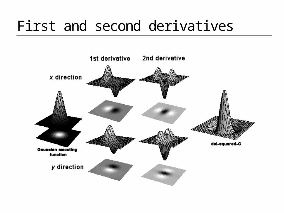
First and second derivatives
* =

First and second derivatives
Original First Derivative x Second Derivative x, y
What are these good for?

Subtracting filters
Original Second Derivative Sharpened

for some
Combining filters
*
*
0 0 0 0 0
0 0 0 0 0
0 -1 0 1 0
0 0 0 0 0
0 0 0 0 0
0 0 0 0 0
0 0 -1 0 0
0 -1 4 -1 0
0 0 -1 0 0
0 0 0 0 0
=
=It’s also true:

Combining Gaussian filters
More blur than either individually (but less than )
* = ?
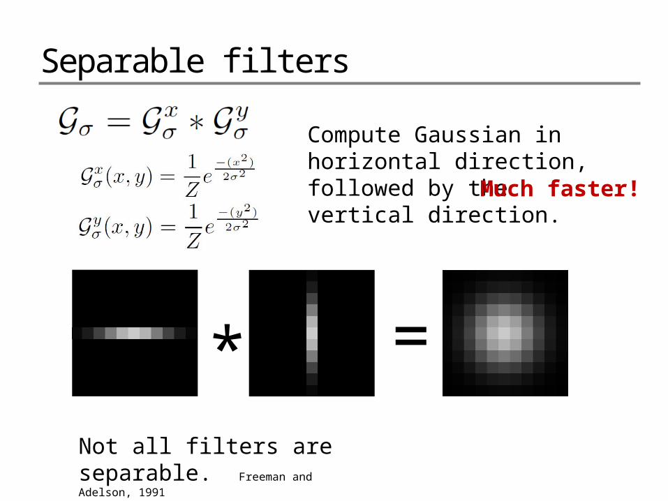
Separable filters
* =
Compute Gaussian in horizontal direction, followed by the vertical direction.
Not all filters are separable. Freeman and Adelson, 1991
Much faster!

Sums of rectangular regions
243 239 240 225 206 185 188 218 211 206 216 225
242 239 218 110 67 31 34 152 213 206 208 221
243 242 123 58 94 82 132 77 108 208 208 215
235 217 115 212 243 236 247 139 91 209 208 211
233 208 131 222 219 226 196 114 74 208 213 214
232 217 131 116 77 150 69 56 52 201 228 223
232 232 182 186 184 179 159 123 93 232 235 235
232 236 201 154 216 133 129 81 175 252 241 240
235 238 230 128 172 138 65 63 234 249 241 245
237 236 247 143 59 78 10 94 255 248 247 251
234 237 245 193 55 33 115 144 213 255 253 251
248 245 161 128 149 109 138 65 47 156 239 255
190 107 39 102 94 73 114 58 17 7 51 137
23 32 33 148 168 203 179 43 27 17 12 8
17 26 12 160 255 255 109 22 26 19 35 24
How do we compute the sum of the pixels in the red box?
After some pre-computation, this can be done in constant time for any box.
This “trick” is commonly used for computing Haar wavelets (a fundemental building block of many object recognition approaches.)

Sums of rectangular regions
The trick is to compute an “integral image.” Every pixel is the sum of its neighbors to the upper left.
Sequentially compute using:
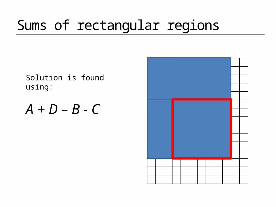
Sums of rectangular regions
A B
C D
Solution is found using:
A + D – B - C

Spatially varying filters
Some filters vary spatially.
Useful for deblurring.
Durand, 02

*
*
*
input output
Same Gaussian kernel everywhere.Slides courtesy of Sylvian Paris
Constant blur

*
*
*
input output
The kernel shape depends on the image content.Slides courtesy of Sylvian Paris
Bilateral filter
Maintains edges when blurring!

Borders
What to do about image borders:
black fixed periodic reflected

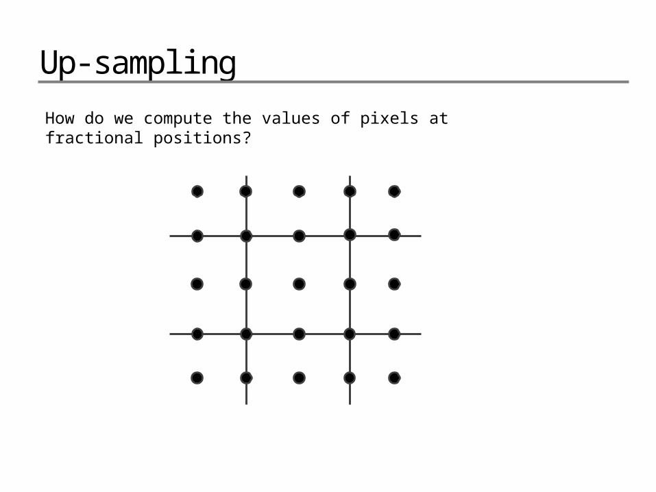
Up-sampling
How do we compute the values of pixels at fractional positions?

Up-sampling
f (x,y) f (x+1,y)
f (x+1,y+1)f (x,y+1)
f (x+0.8,y+0.3) f (x + a, y + b) = (1 - a)(1 - b) f (x, y) + a(1 - b) f (x + 1, y) + (1 - a)b f (x,y + 1) + ab f (x + 1, y + 1)
Bilinear sampling:
Bicubic sampling fits a higher order function using a larger area of support.
How do we compute the values of pixels at fractional positions?

Up-sampling
Nearest neighbor Bilinear Bicubic

Down-sampling
If you do it incorrectly your images could look like this:
Check out Moire patterns on the web.

Down-sampling
• Aliasing can arise when you sample a continuous signal or image– occurs when your sampling rate is not high enough to capture the
amount of detail in your image– Can give you the wrong signal/image—an alias– formally, the image contains structure at different scales
• called “frequencies” in the Fourier domain– the sampling rate must be high enough to capture the highest frequency
in the image
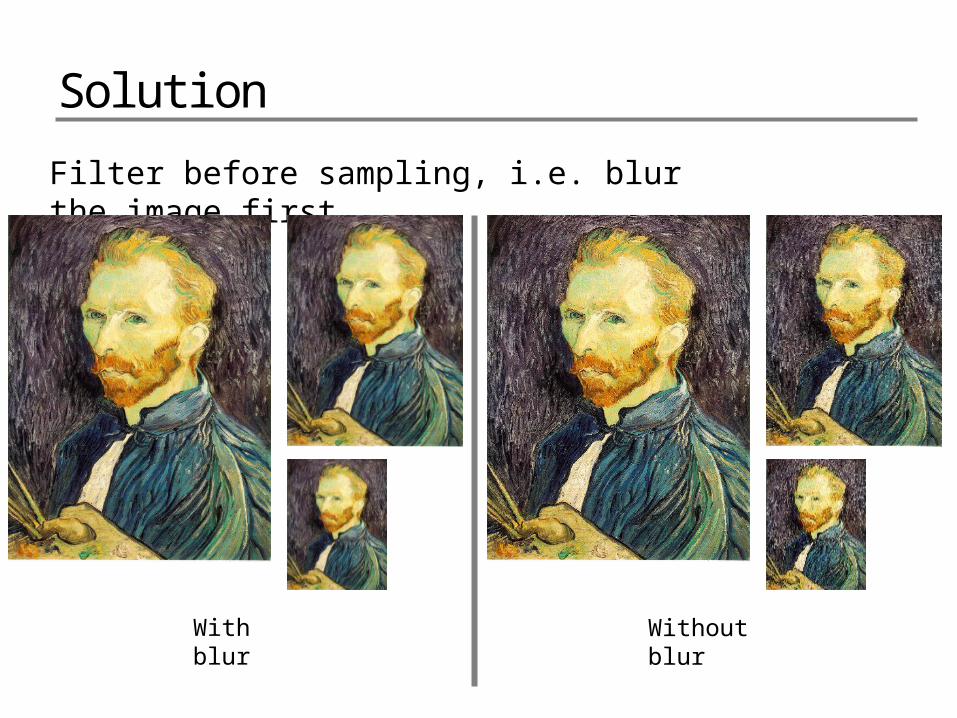
Solution
Filter before sampling, i.e. blur the image first.
With blur Without blur