remote sensing

Article

Filling the Polar Data Gap in Sea Ice ConcentrationFields Using Partial Differential Equations

Courtenay Strong 1,* and Kenneth M. Golden 2

1 Department of Atmospheric Sciences, University of Utah, 135 S 1460 E, Rm 819, Salt Lake City, UT 84112,USA

2 Department of Mathematics, University of Utah, 155 S 1400 E, RM 233, Salt Lake City, UT 84112, USA;golden@math.utah.edu

* Correspondence: court.strong@utah.edu; Tel.: +1-801-585-0049; Fax: +1-801-585-3681

Academic Editors: Walt Meier, Mark Tschudi, Xiaofeng Li, Raphael M. Kudela and Prasad S. ThenkabailReceived: 28 February 2016; Accepted: 18 May 2016; Published: date

Abstract: The “polar data gap” is a region around the North Pole where satellite orbit inclination andinstrument swath for SMMR and SSM/I-SSMIS satellites preclude retrieval of sea ice concentrations.Data providers make the irregularly shaped data gap round by centering a circular “pole holemask” over the North Pole. The area within the pole hole mask has conventionally been assumedto be ice-covered for the purpose of sea ice extent calculations, but recent conditions around theperimeter of the mask indicate that this assumption may already be invalid. Here we proposean objective, partial differential equation based model for estimating sea ice concentrations withinthe area of the pole hole mask. In particular, the sea ice concentration field is assumed to satisfyLaplace’s equation with boundary conditions determined by observed sea ice concentrations on theperimeter of the gap region. This type of idealization in the concentration field has already provedto be quite useful in establishing an objective method for measuring the “width” of the marginal icezone—a highly irregular, annular-shaped region of the ice pack that interacts with the ocean, andtypically surrounds the inner core of most densely packed sea ice. Realistic spatial heterogeneityin the idealized concentration field is achieved by adding a spatially autocorrelated stochasticfield with temporally varying standard deviation derived from the variability of observationsaround the mask. To test the model, we examined composite annual cycles of observation-modelagreement for three circular regions adjacent to the pole hole mask. The composite annual cycle ofobservation-model correlation ranged from approximately 0.6 to 0.7, and sea ice concentration meanabsolute deviations were of order 10−2 or smaller. The model thus provides a computationallysimple approach to solving the increasingly important problem of how to fill the polar datagap. Moreover, this approach based on solving an elliptic partial differential equation with givenboundary conditions has sufficient generality to also provide more sophisticated models whichcould potentially be more accurate than the Laplace equation version. Such generalizations andpotential validation opportunities are discussed.

Keywords: sea ice; interpolation; passive microwave

1. Introduction

Declines in Arctic sea ice provide some of the most compelling evidence of climate change, andquantitative assessment of sea ice trends from 1979 to the present relies heavily on satellite-basedpassive microwave retrievals of sea ice concentrations [1,2]. The satellite platforms used to observethese long-term concentration trends are the Special Sensor Microwave Imager/Sounder (SSMIS) andits two predecessors: the Special Sensor Microwave/Imager (SSM/I), and the Scanning MultichannelMicrowave Radiometer (SMMR). Data from these platforms suffer from a “polar data gap,” which

Remote Sens. 2016, xx, x; doi:10.3390/—— www.mdpi.com/journal/remotesensing

Remote Sens. 2016, xx, x 2 of 10

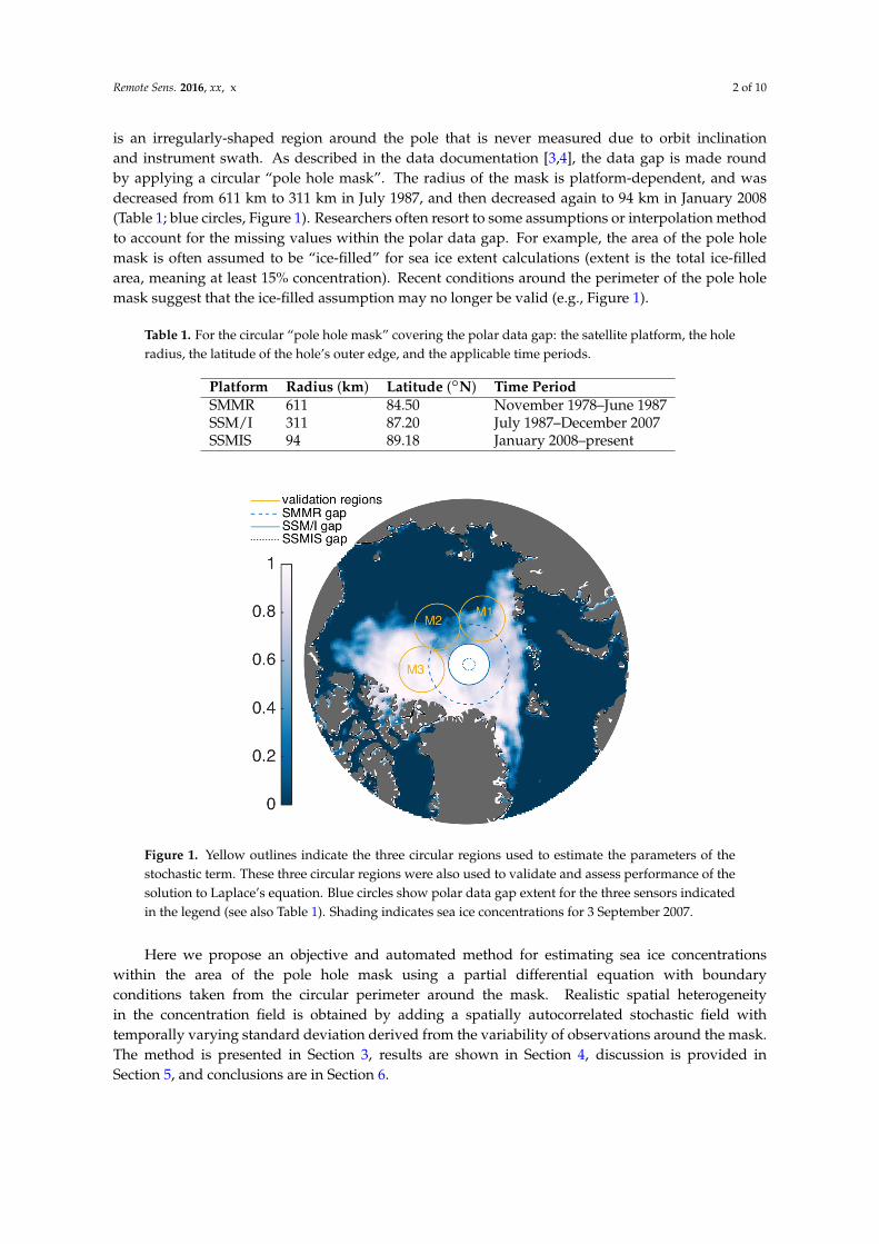
is an irregularly-shaped region around the pole that is never measured due to orbit inclinationand instrument swath. As described in the data documentation [3,4], the data gap is made roundby applying a circular “pole hole mask”. The radius of the mask is platform-dependent, and wasdecreased from 611 km to 311 km in July 1987, and then decreased again to 94 km in January 2008(Table 1; blue circles, Figure 1). Researchers often resort to some assumptions or interpolation methodto account for the missing values within the polar data gap. For example, the area of the pole holemask is often assumed to be “ice-filled” for sea ice extent calculations (extent is the total ice-filledarea, meaning at least 15% concentration). Recent conditions around the perimeter of the pole holemask suggest that the ice-filled assumption may no longer be valid (e.g., Figure 1).

Table 1. For the circular “pole hole mask” covering the polar data gap: the satellite platform, the holeradius, the latitude of the hole’s outer edge, and the applicable time periods.

Platform Radius (km) Latitude (N) Time PeriodSMMR 611 84.50 November 1978–June 1987SSM/I 311 87.20 July 1987–December 2007SSMIS 94 89.18 January 2008–present

Figure 1. Yellow outlines indicate the three circular regions used to estimate the parameters of thestochastic term. These three circular regions were also used to validate and assess performance of thesolution to Laplace’s equation. Blue circles show polar data gap extent for the three sensors indicatedin the legend (see also Table 1). Shading indicates sea ice concentrations for 3 September 2007.

Here we propose an objective and automated method for estimating sea ice concentrationswithin the area of the pole hole mask using a partial differential equation with boundaryconditions taken from the circular perimeter around the mask. Realistic spatial heterogeneityin the concentration field is obtained by adding a spatially autocorrelated stochastic field withtemporally varying standard deviation derived from the variability of observations around the mask.The method is presented in Section 3, results are shown in Section 4, discussion is provided inSection 5, and conclusions are in Section 6.

Remote Sens. 2016, xx, x 3 of 10

2. Data

We explored filling the polar data gap in three principal passive microwave sea ice concentrationdata sets from the National Snow and Ice Data Center (NSIDC): concentrations based on the Bootstrapalgorithm [5], concentrations based on the National Aeronautics and Space Administration (NASA)Team algorithm [6], and concentrations from the Climate Data Record of Passive Microwave Sea IceConcentration (CDR) which is a blending of different algorithms intended to produce a consistentrecord over time [4]. The presented analyses use the NASA Team algorithm, which tends toproduce lower concentrations [7], and hence more challenging cases for filling the polar data gap(i.e., boundary concentrations uniformly close to 1.0 can be realistically treated with more trivialinterpolation). Using the other two data sets (bootstrap and CDR), the proposed model performedcomparably (not shown) to the NASA Team algorithm data results presented in Section 4.

3. Method

3.1. Formulation of Data Fill Model

In prior publications (e.g., [8]), we filled the polar data gap (region here denoted G) usingmethods based on “thin plate splines” or other radial basis functions [9]. In exploring alternativemethods for the present study, we also experimented with techniques similar to a modifiedspherical Shepard’s interpolant [10] and various planar multiquadric methods [11]. These familiesof interpolation techniques can produce seemingly realistic fills at modest computational expense,but we are here interested in presenting and exploring advantages of fills based on solutions topartial differential equations. Specifically, we investigate ideas emerging from “inpainting” or“disocclusion” techniques [12], meaning that a partial differential equation (PDE) is solved in adomain to replace missing data within its perimeter, given known boundary conditions on theperimeter. Here, we propose to model the sea ice concentration field ( f ) in a region G on Earth’ssurface, the pole hole mask, as the sum of two functions

f (λ, φ) = ψ(λ, φ) + Ω(λ, φ) (1)

where λ is longitude and φ is latitude, or f (~r) = ψ(~r) + Ω(~r) where ~r ∈ G. The scalar field ψ isassumed to be a solution of Laplace’s equation

∇2ψ = 0 (2)

in spherical coordinates, and Ω is a stochastic term that provides realistic spatial heterogeneityassociated with deviations of the concentration field from ψ. We show below that Ω estimatedfrom observations exhibits a characteristic spatial autocorrelation, and we incorporate this into itsformulation (Section 3.2).

Dirichlet boundary conditions for ψ are obtained from ice concentration data on the pole holemask boundary ∂G. Then a unique harmonic function ψ, satisfying Equation (2), exists if ∂G issufficiently smooth and the ice concentration is a continuous function along ∂G. Using m to denotethe number of grid points within the mask, we have m unknown sea ice concentrations for eachday. Expressing the Laplacian as a second-order finite difference operator gives m linear equationsin m unknowns with boundary conditions specified by the concentrations on ∂G. The unknownconcentrations are then obtained using computationally efficient methods for solving sparse linearsystems [13]. For convenience, we hereafter work with the Cartesian coordinates (x, y) of the polarstereographic projection used by NSIDC. This projection is a conformal mapping, so ψ(x, y) alsosolves Laplace’s equation when projected back onto the sphere as ψ(λ, φ).

Remote Sens. 2016, xx, x 4 of 10

3.2. Stochastic Term Ω

Satellite-retrieved sea ice concentration fields contain noise or uncertainty associated with thepassive microwave retrieval algorithms, and also heterogeneity due to physical processes such asmelt pond formation and the various thermodynamic and dynamic controls on concentration [14].Here, we model Ω as spatially correlated, zero-mean additive Gaussian noise with two parameters:σ, the standard deviation of the surface amplitude, and η, the spatial autocorrelation length scale.They are both estimated using data from regions near the pole hole mask (yellow circles M1–M3,Figure 1). These circles were chosen to be the size of the SSM/I pole hole mask used for the majorityof the record (Table 1), they were positioned close to the pole hole mask but away from regions whereopen ocean is common, and they were arranged so as to be non-overlapping. The parameter σ has astrong annual cycle as shown below, but is assumed spatially uniform on any given day of year.

For each day of the year, we collected three samples of the stochastic function Ω by first solvingLaplace’s equation to obtain ψ within each of the circular regions M1–M3 in Figure 1. Given thesolution ψ, we then solved Equation (1) to obtain a sample stochastic field Ωs via

Ωs(~r) = fobs(~r)− ψ(~r), ~r ∈ Mj, j = 1, 2, 3 (3)

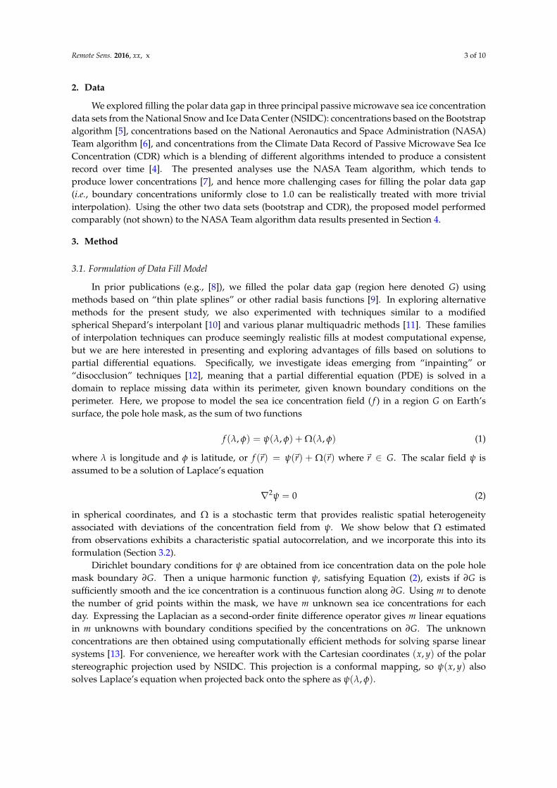
where fobs(~r),~r ∈ Mj is the observed sea ice field from region Mj, j = 1,2,3. The spatial standarddeviation of Ωs for all the M regions displayed together (Figure 2) motivates a model of σ with highervalues in the melt season. Specifying that t denotes decimal day of the year, the model

σ = σ0 +nk

∑k=1

[αk cos(2πk(t− 1)/364) + βk sin(2πk(t− 1)/364)] (4)

accounts for 52% of the variation in σ with nk = 2, σ0 = 2.3× 10−2, (α1, α2) = (−1.3,−1.8)× 10−3,and (β1, β2) = (−1.7, 6.8)× 10−3.

day of year0 50 100 150 200 250 300 350

σ

0

0.02

0.04

0.06

0.08

0.1

0.12

Figure 2. Circles indicate empirical estimates of the standard deviation σ of the stochastic term Ω,as a function of day of the year for 1988–2013, where 1988 is selected because it is the first full yearafter adoption of the moderately-sized pole hole mask (radius 311 km, Table 1). The curve is a fit ofEquation (4) with k = 2. Values exceeding 0.12 (less than 1% of the data) are not shown, but wereincluded in the curve fit.

Remote Sens. 2016, xx, x 5 of 10

We defined η as the spatial autocorrelation e-folding distance, and we calculated it for each rowand column of grid points in the smallest square capturing M1, M2, or M3 for each day of the year for1988–2013. The parameter η had neither a strong annual cycle nor a strong anisotropy (e.g., averaged60 km versus 62 km in two orthogonal directions), and we prescribed η to be 61 km.

To generate a realization of Ω, we produced a field of spatially uncorrelated Gaussian noiseΓ(x, y) with standard deviation σ. We then introduced the desired spatial autocorrelation byconvolution of Γ with the Gaussian function

g = exp

[− (x2 + y2)

2( η

2)2

](5)

which yields η as the autocorrelation e-folding length scale (e.g., [15]). The full field Ω is defined by

Ω(x, y) =2h

η√

πF−1 F Γ(x, y) · F g(x, y) (6)

where the convolution [Γ(x, y) ∗ g(x, y)] is achieved via Fourier transform F for computationalefficiency, the symbol · denotes point-wise multiplication, h is the grid spacing, and the coefficient2h/(η

√π) is included to approximately recover σ as the root mean square amplitude of Ω. Having

calculated a solution ψ and a stochastic realization Ω, we restricted concentration to the range0 ≤ c ≤ 1 by imposing

f =

ψ + Ω where 0 ≤ ψ + Ω ≤ 1

1 where ψ + Ω > 1

0 where ψ + Ω < 0.

(7)

4. Results

4.1. Illustrative Examples

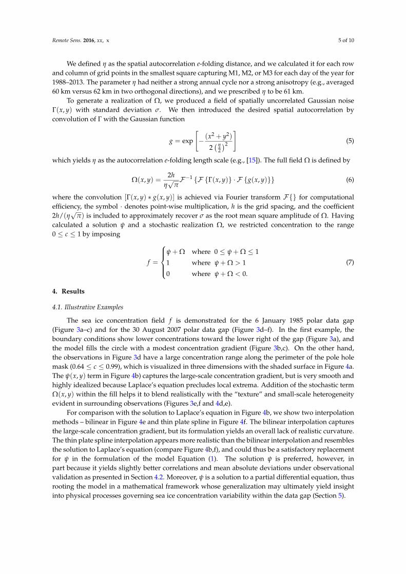
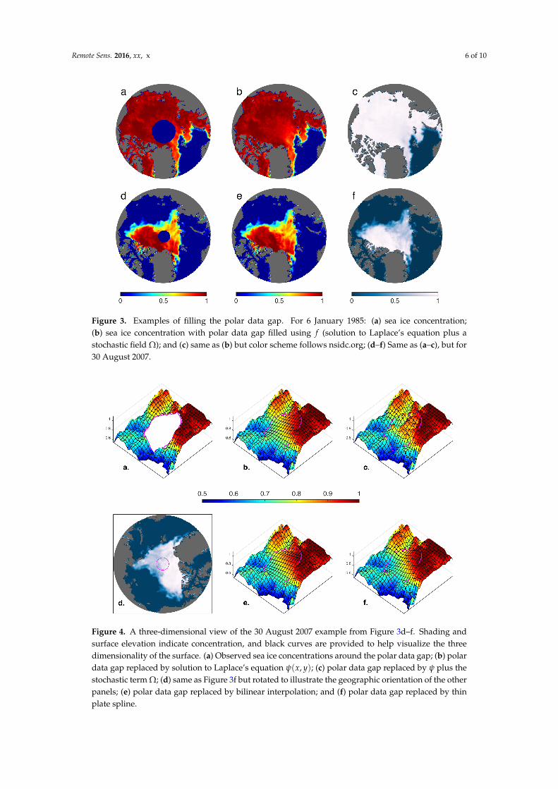
The sea ice concentration field f is demonstrated for the 6 January 1985 polar data gap(Figure 3a–c) and for the 30 August 2007 polar data gap (Figure 3d–f). In the first example, theboundary conditions show lower concentrations toward the lower right of the gap (Figure 3a), andthe model fills the circle with a modest concentration gradient (Figure 3b,c). On the other hand,the observations in Figure 3d have a large concentration range along the perimeter of the pole holemask (0.64 ≤ c ≤ 0.99), which is visualized in three dimensions with the shaded surface in Figure 4a.The ψ(x, y) term in Figure 4b) captures the large-scale concentration gradient, but is very smooth andhighly idealized because Laplace’s equation precludes local extrema. Addition of the stochastic termΩ(x, y) within the fill helps it to blend realistically with the “texture” and small-scale heterogeneityevident in surrounding observations (Figures 3e,f and 4d,e).

For comparison with the solution to Laplace’s equation in Figure 4b, we show two interpolationmethods – bilinear in Figure 4e and thin plate spline in Figure 4f. The bilinear interpolation capturesthe large-scale concentration gradient, but its formulation yields an overall lack of realistic curvature.The thin plate spline interpolation appears more realistic than the bilinear interpolation and resemblesthe solution to Laplace’s equation (compare Figure 4b,f), and could thus be a satisfactory replacementfor ψ in the formulation of the model Equation (1). The solution ψ is preferred, however, inpart because it yields slightly better correlations and mean absolute deviations under observationalvalidation as presented in Section 4.2. Moreover, ψ is a solution to a partial differential equation, thusrooting the model in a mathematical framework whose generalization may ultimately yield insightinto physical processes governing sea ice concentration variability within the data gap (Section 5).

Remote Sens. 2016, xx, x 6 of 10

Figure 3. Examples of filling the polar data gap. For 6 January 1985: (a) sea ice concentration;(b) sea ice concentration with polar data gap filled using f (solution to Laplace’s equation plus astochastic field Ω); and (c) same as (b) but color scheme follows nsidc.org; (d–f) Same as (a–c), but for30 August 2007.

Figure 4. A three-dimensional view of the 30 August 2007 example from Figure 3d–f. Shading andsurface elevation indicate concentration, and black curves are provided to help visualize the threedimensionality of the surface. (a) Observed sea ice concentrations around the polar data gap; (b) polardata gap replaced by solution to Laplace’s equation ψ(x, y); (c) polar data gap replaced by ψ plus thestochastic term Ω; (d) same as Figure 3f but rotated to illustrate the geographic orientation of the otherpanels; (e) polar data gap replaced by bilinear interpolation; and (f) polar data gap replaced by thinplate spline.

Remote Sens. 2016, xx, x 7 of 10

4.2. Validation and Performance Assessment

To validate the data fill model and assess performance, we generated ψ for the three regionsM1–M3 (Figure 1) for each day of the year from 1988–2013. Because Ω in Equation (1) is stochastic,it has zero correlation with observations, so the performance analysis is on ψ rather than the fullf . Our validation method assumes that the three selected regions near the polar data gap arerepresentative of concentration conditions within the gap itself. Validation results are presented foreach region as composite annual cycles (Figure 5), meaning values were averaged across years toproduce one value for each day of the year.

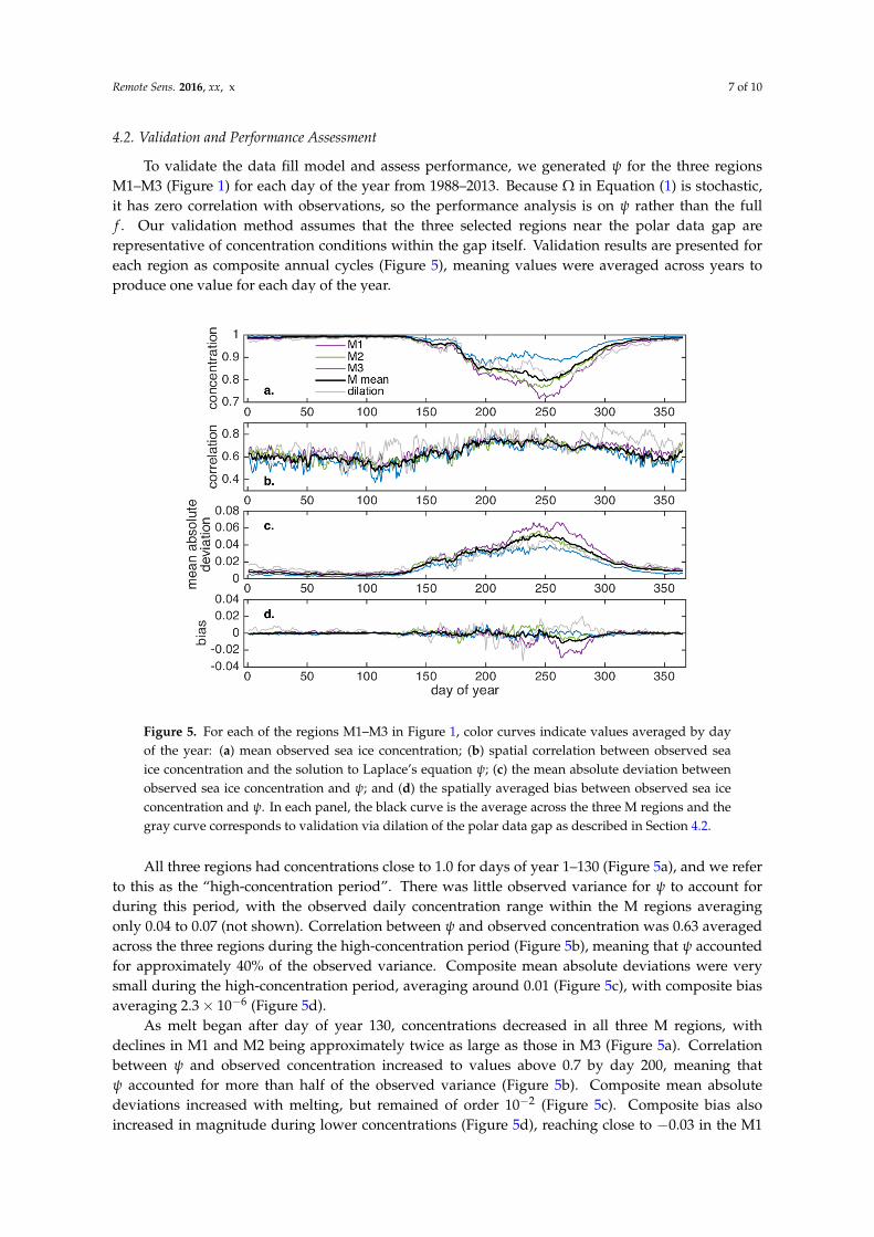
Figure 5. For each of the regions M1–M3 in Figure 1, color curves indicate values averaged by dayof the year: (a) mean observed sea ice concentration; (b) spatial correlation between observed seaice concentration and the solution to Laplace’s equation ψ; (c) the mean absolute deviation betweenobserved sea ice concentration and ψ; and (d) the spatially averaged bias between observed sea iceconcentration and ψ. In each panel, the black curve is the average across the three M regions and thegray curve corresponds to validation via dilation of the polar data gap as described in Section 4.2.

All three regions had concentrations close to 1.0 for days of year 1–130 (Figure 5a), and we referto this as the “high-concentration period”. There was little observed variance for ψ to account forduring this period, with the observed daily concentration range within the M regions averagingonly 0.04 to 0.07 (not shown). Correlation between ψ and observed concentration was 0.63 averagedacross the three regions during the high-concentration period (Figure 5b), meaning that ψ accountedfor approximately 40% of the observed variance. Composite mean absolute deviations were verysmall during the high-concentration period, averaging around 0.01 (Figure 5c), with composite biasaveraging 2.3× 10−6 (Figure 5d).

As melt began after day of year 130, concentrations decreased in all three M regions, withdeclines in M1 and M2 being approximately twice as large as those in M3 (Figure 5a). Correlationbetween ψ and observed concentration increased to values above 0.7 by day 200, meaning thatψ accounted for more than half of the observed variance (Figure 5b). Composite mean absolutedeviations increased with melting, but remained of order 10−2 (Figure 5c). Composite bias alsoincreased in magnitude during lower concentrations (Figure 5d), reaching close to −0.03 in the M1

Remote Sens. 2016, xx, x 8 of 10

region on day of year 264 because local maxima of concentration formed on the interior of this regionduring several of the analyzed years (recall that the solution to Laplace’s equation precludes localextrema). Averaged across the three M regions, the composite bias remained smaller than 1.2× 10−2

in magnitude and averaged 9.9× 10−4 overall (black curve, Figure 5d).As an additional validation, we also dilated the SSMIS 94-km radius gap to the 311-km radius

of its SSMI/I predecessor, and compared modeled and observed concentrations within the 311-kmradius region (the 94-km and 311-km radius gaps are indicated by dotted and solid blue circles,respectively, Figure 1). This dilation-based validation has more sampling variability than theM-region analysis because the 94-km radius is available for only 2008–2015, but the results are similarfor the two validations (gray curves, Figure 5).

As noted in Section 4.1, a thin plate spline could provide a reasonable substitute for ψ in themodel formulation (compare Figure 4b,f). We repeated the above-described observational validationprocedure for the M regions, but now replacing ψ with a thin plate spline, and found a slightdegradation in overall performance. Specifically, correlation averaged r = 0.56 for the thin platespline versus r = 0.64 for ψ, and the overall mean absolute deviation was approximately 8% largerfor the thin plate spline (not shown).

5. Discussion

The model proposed here is toward the simpler end of the spectrum of possible methods.An even simpler fill method could replace the solution to Laplace’s equation (ψ in Equation (1)) witha linear function of the form

ψlin(x, y) = γ1x + γ2y + γ3, (8)

where the γ parameters minimize, for example, the sum of squared deviations from observationsalong the gap’s perimeter. The simplest possible model would be the special case of Equation (8)where γ1 = γ2 = 0, meaning the gap is filled by a constant. Using a PDE such as Laplace’s equationenables the solution to agree with observations on the boundary ∂G, which is clearly desirable.We could instead specify the normal derivative of concentration on the boundary rather thanthe concentration itself (i.e., impose Neumann boundary conditions), but then existence imposesrestrictions on the derivative and we have uniqueness only up to a constant.

If we progress in complexity beyond the model proposed here, we could considergeneralizations of Laplace’s equation such as Poisson’s equation or time-dependent formulations.The incorporation of a local conductivity or diffusivity field D(x, y), written

∇ · (D∇ψ) = 0, (9)

would enable the PDE portion of the model (ψ) to accommodate a much broader class ofconcentration features including local extrema precluded by Laplace’s equation. At maximalconceptual complexity, and perhaps also maximal computational expense, we havedynamic-thermodynamic sea ice models that simulate evolution of fractional ice coverage acrossmultiple thickness classes, and it would be possible to fill the polar data gap using this class ofmodels along with suitable initial and boundary conditions.

We also sought relative simplicity in our treatment of the stochastic term Ω(x, y). Its amplitudeclearly motivated a time-dependent standard deviation, but we assumed this parameter washomogeneous in space for any given day of the year. Observations moreover supported a relativelysimple isotropic autocorrelation e-folding length scale η for the stochastic term. The precedingproduces realistic results suitable for displaying single maps or initializing a simulation. Otherapplications may motivate a more sophisticated treatment where the stochastic term is an evolvingspace-time field Ω(x, y, t) with temporal as well as spatial autocorrelation, and this model couldbe estimated as, for example, a vector autoregressive process. Finally, our formulation of the

Remote Sens. 2016, xx, x 9 of 10

stochastic term uses parameters (η and σ) that are empirically estimated from observations, andfurther advances in realism may be possible by adjusting parameters of the stochastic realizationto reflect, for example, surrounding variance and anisotropy in the observed ice field.

The availability of concentration data within the pole hole mask now or in the future presentsan opportunity to enhance the proposed model. Examples of data available now include valueswithin the irregular edge of the polar data gap that are currently covered by the circular pole holemask, but their inclusion may invalidate the assumption that the perimeter ∂G is sufficiently smooth.Considering hypothetical data sets, a single measurement at the pole could provide an additionalDirichlet boundary condition for solving Laplace’s equation. If the new data are distributed sparselyacross the gap, they could pair with the boundary conditions around the perimeter to inform aleast-squares solution to Laplace’s equation or, perhaps more effectively, to inform the stochasticheterogeneity field that is added to the solution to Laplace’s equation.

6. Conclusions

A conceptually and computationally simple model was proposed for objective, automated fillingof the polar data gap in passive microwave sea ice concentration data. The formulation of themodel is largely a solution to a PDE (here we used Laplace’s equation) with boundary conditionstaken from the circular perimeter of the pole hole mask. The solution of the PDE was added to aspatially autocorrelated, additive Gaussian white noise that mimics the spatial heterogeneity evidentin surrounding observations of sea ice concentration. The standard deviation of the stochastic termfit to observations had a prominent annual cycle, with maxima during low sea ice concentrations.The stochastic term has cosmetic utility, helping the fill data to blend naturally with surroundingobservations, and it also provides a realistic spatial heterogeneity enabling observations to be used asinitial conditions for simulation.

The fill also enables objective treatment of the missing data for the purpose of calculating extentand area trends. The polar data gap has conventionally been assumed to be ice-covered for thepurpose of extent calculations, but recent conditions around the perimeter of the gap indicate thatthis assumption may already be invalid. Fortunately, the trend toward lower concentrations nearthe pole has been accompanied by two substantial reductions in the radius of the pole hole mask,mitigating uncertainty associated with the assumptions made in treating the missing data. Basedon validation and skill assessment in circular regions around the pole hole mask, the PDE portionof the fill maintains composite mean absolute deviations of order 10−2 or smaller, and accounts for40%–50% of the variance in observed concentrations depending on region.

Acknowledgments: The authors gratefully acknowledge support from the Division of Mathematical Sciencesat the U.S. National Science Foundation (NSF) through Grants DMS-1413454 and DMS-0940249. We also thankthe NSF Math Climate Research Network for their support of this work. Three anonymous reviewers providedcomments that helped to improve an earlier version of the manuscript.

Author Contributions: Courtenay Strong and Kenneth Golden conceived the research project and contributedto writing the manuscript. Courtenay Strong performed the coding and data analysis.

Conflicts of Interest: The authors declare no conflict of interest.

References

1. Cavalieri, D.J.; Parkinson, C.L. Arctic sea ice variability and trends, 1979–2010. Cryosphere 2012, 6, 881–889.2. Simmonds, I. Comparing and contrasting the behavior of Arctic and Antarctic sea ice over the 35 year

period 1979–2013. Ann. Glaciol. 2015, 56, 18–28.3. Cavalieri, D.; Parkinson, C.; Gloersen, P.; Zwally, H.J. Sea Ice Concentrations from Nimbus-7 SMMR and DMSP

SSM/I Passive Microwave Data. National Snow and Ice Data Center: Boulder, CO, USA, 1996.4. Meier, W.; Fetterer, F.; Savoie, M.; Mallory, S.; Duerr, R.; Stroeve, J. NOAA/NSIDC Climate Data Record of

Passive Microwave Sea Ice Concentration. National Snow and Ice Data Center: Boulder, CO, USA, 2011.5. Comiso, J.C. Characteristics of arctic winter sea ice from satellite multispectral microwave observations.

J. Geophys. Res. 1986, 91, 975–994.

Remote Sens. 2016, xx, x 10 of 10

6. Cavalieri, D.J.; Gloersen, P.; Campbell, W.J. Determination of sea ice parameters with the NIMBUS 7 SMMR.J. Geophys. Res. 1984, 89, 5355–5369.

7. Notz, D. Sea-ice extent and its trend provide limited metrics of model performance. Cryosphere 2014,8, 229–243.

8. Strong, C.; Rigor, I.G. Arctic marginal ice zone trending wider in summer and narrower in winter. Geophys.Res. Lett. 2013, 40, 4864–4868.

9. Duchon, J. Splines minimizing rotation-invariant semi-norms in Sobolev spaces. In Constructive Theoryof Functions of Several Variables; Springer: Berlin, Germany; Heidelberg, Germany, 1977; Volume 571,pp. 85–100.

10. Cavoretto, R.; De Rossi, A. Fast and accurate interpolation of large scattered data sets on the sphere.J. Comput. Appl. Math. 2010, 234, 1505–1521.

11. Pottmann, H.; Eck, M. Modified multiquadric methods for scattered data interpolation over a sphere.Computer Aided Geometr. Des. 1990, 7, 313–321.

12. Arias, P.; Facciolo, G.; Caselles, V.; Sapiro, G. A Variational Framework for Exemplar-Based ImageInpainting. Int. J. Computer Vis. 2011, 93, 319–347.

13. Gilbert, J.R.; Moler, C.; Schreiber, R. Sparse Matrices in MATLAB: Design and Implementation. SIAM J.Matrix Anal. Appl. 1992, 13, 333–356.

14. Carsey, F.D. Microwave Remote Sensing of Sea Ice; American Geophysical Union: Washington, DC, USA,1992; p. 462.

15. Garcia, N.; Stoll, E. Monte Carlo Calculation for Electromagnetic-Wave Scattering from Random RoughSurfaces. Phys. Rev. Lett. 1984, 52, 1798–1801.

c© 2016 by the authors; licensee MDPI, Basel, Switzerland. This article is an open accessarticle distributed under the terms and conditions of the Creative Commons Attribution(CC-BY) license (http://creativecommons.org/licenses/by/4.0/).