Field and Lab Convergence in Poisson LUPI Games�

Robert Östlingy Joseph Tao-yi Wangz Eileen Choux

Colin F. Camerer{

SSE/EFI Working Paper Series in Economics and Finance No. 671

This version: October 30, 2007

�The �rst two authors, Joseph Tao-yi Wang and Robert Östling, contributed equally to this paper. Weare grateful for helpful comments from Tore Ellingsen, Magnus Johannesson, Botond Köszegi, David Laib-son, Erik Lindqvist, Stefan Molin, Noah Myung, Rosemarie Nagel, Charles Noussair, Carsten Schmidt,Dmitri Vinogradov, Mark Voorneveld, Jörgen Weibull, seminar participants at California Institute ofTechnology, Stockholm School of Economics, Mannheim Empirical Research Summer School 2007, andUC Santa Barbara Cognitive Neuroscience Summer School 2007. Robert Östling acknowledges �nancialsupport from the Jan Wallander and Tom Hedelius Foundation. Colin Camerer acknowledges supportfrom the NSF HSD program, HSFP, and the Betty and Gordon Moore Foundation.

yDepartment of Economics, Stockholm School of Economics, P.O. Box 6501, SE�113 83 Stockholm,Sweden. E-mail: robert.ostling@hhs.se.

zDepartment of Economics, National Taiwan University, 21 Hsu-Chow Road, Taipei 100, Taiwan.E-mail: josephw@ntu.edu.tw.

xManagement and Organization, Kellogg School of Management, Northwestern University, EvanstonIL 60201, USA. E-mail: e-chou@kellogg.northwestern.edu.

{Division for the Humanities and Social Sciences, MC 228-77, California Institute of Technology,Pasadena CA 91125, USA. E-mail: camerer@hss.caltech.edu.

Abstract

In the lowest unique positive integer (LUPI) game, players pick positive integers and the

player who chose the lowest unique number (not chosen by anyone else) wins a �xed

prize. We derive theoretical equilibrium predictions, assuming fully rational players with

Poisson-distributed uncertainty about the number of players. We also derive predictions

for boundedly rational players using quantal response equilibrium and a cognitive hier-

archy of rationality steps with quantal responses. The theoretical predictions are tested

using both �eld data from a Swedish gambling company, and laboratory data from a

scaled-down version of the �eld game. The �eld and lab data show similar patterns: in

early rounds, players choose very low and very high numbers too often, and avoid focal

(�round�) numbers. However, there is some learning and a surprising degree of conver-

gence toward equilibrium. The cognitive hierarchy model with quantal responses can

account for the basic discrepancies between the equilibrium prediction and the data.

jel classification: C72, C92, L83, C93.

keywords: Population uncertainty, Poisson game, QRE, congestion game, guessing

game, experimental methods, behavioral game theory, cognitive hierarchy.

1 Introduction

In early 2007, a Swedish gambling company introduced a simple lottery. In the lottery,

players simultaneously choose positive integers from 1 to K. The winner is the player

who chooses the lowest number that nobody else picked. We call this the LUPI game1,

because the lowest unique positive integer wins. This paper analyzes LUPI theoretically

and reports data from the Swedish �eld experience and from parallel lab experiments.

LUPI is not an exact model of anything in the political economy, but it combines

strategic features of other important naturally-occurring games. For example, in games

with congestion, a player�s payo¤s are lower if others choose the same strategy. Examples

include choices of tra¢ c routes and research topics, or buyers and sellers choosing among

multiple markets. LUPI has the property of an extreme congestion game, in which having

even one other player choose the same number reduces one�s payo¤to zero. However, LUPI

is not a congestion game as de�ned by Rosenthal (1973) since the payo¤ from choosing

a particular number does not only depend on how many other players that picked that

number, but also on how many that picked lower numbers.

The closest analogues to LUPI in the economy are unique bid auctions (see the ongoing

research by Eichberger and Vinogradov, 2007, Raviv and Virag, 2007 and Rapoport,

Otsubo, Kim, and Stein, 2007). In these auctions, an object is sold either to the lowest

bidder whose bid is unique, or in some versions of the auction to the highest unique bid.

LUPI di¤ers from these auctions in that players don�t have to pay their bid if they win and

also avoids complications resulting from private valuations. LUPI focuses on the essential

strategic con�ict: players want to choose low numbers, in order to be the lowest, but also

want to avoid numbers others will choose, in order to be unique.

While LUPI is an arti�cial game that was not designed to model a familiar economic

situation, it is interesting to study for several reasons.

First, since game-theoretic reasoning is generally hoped to apply universally across

many classes of games, studying its application in an arti�cial game (where predictions

are clear and bold) is scienti�cally useful. And since the number of players who participate

in the Swedish lottery is not �xed, analyzing the LUPI game presents an opportunity to

empirically test theory in which the number of players is Poisson-distributed (Myerson,

1998) for the �rst time.2

Second, the clear structure of the Swedish LUPI lottery allows us to create a parallel

lab experiment. This parallelism provides a rare opportunity to see whether an experiment

1The Swedish company called the game Limbo, but we think LUPI is more apt and mnemonic.2This also distinguishes our paper from the research on unique bid auctions by Eichberger and Vino-

gradov (2007), Raviv and Virag (2007) and Rapoport, Otsubo, Kim, and Stein (2007) which all assumethat the number of players is �xed and commonly known.

1

deliberately designed to replicate the empirical regularities observed in a particular �eld

setting can lead to comparable �ndings. The �eld and lab conclusions are very similar.

The strengths of each of the lab and �eld methods also compensate for weaknesses in the

other method. In the �eld data, there is no way of knowing if the assumption that the

number of players is Poisson-distributed is plausible, whether there is collusion, and how

individual players di¤er and learn. All these concerns can be controlled for or measured

in the lab. In the lab, it is expensive to produce a large sample; there is substantially

more data from the �eld (more than two million choices).

Third, the simple structure of the LUPI game means it is possible to compare Poisson-

equilibrium predictions with precise predictions of two parametric models of boundedly

rational play� quantal response equilibrium, and a level-k cognitive hierarchy approach.

The �eld and lab choices are reasonably close to those predicted by equilibrium. However,

players typically choose more low and high numbers than predicted, and the cognitive

hierarchy approach can account for those deviations.

The next section provides a theoretical analysis of a simple form of the LUPI game,

including the (symmetric) Poisson-Nash equilibrium, quantal response equilibrium and

cognitive hierarchy behavioral models. Section 3 and 4 analyze the data from the �eld

and the lab, respectively. Section 5 discusses the issues concerning �eld vs. lab, and

section 6 concludes the paper.

2 Theory

In the simplest form of LUPI, the number of players, N , has a known distribution, the

players choose integers from 1 to K simultaneously, and the lowest unique number wins.

The winner earns a payo¤ of 1, while all others earn 0.3

We�rst analyze the game when players are assumed to be fully rational, best-responding,

and have equilibrium beliefs. We focus on symmetric equilibria since players both in the

�eld and lab are generally anonymous to each other. We also assume the number of

players is a random variable that has a Poisson distribution, which is a plausible ap-

proximation (and can be exactly implemented in the lab) and much easier to work with

analytically.4 Appendix A and B discusses the �xed-n equilibrium and why it is so much

3In this stylized case, we assume that if there is no lowest unique number there is no winner. Thissimpli�es the analysis because it means that only the probability of being unique must be computed. Inthe Swedish game, if there is no unique number then the players who picked the least-frequently-chosennumber share the top prize. This is just one of many small di¤erences between the simpli�ed gameanalyzed in this section and the game as played in the �eld, which are discussed further below.

4Players did not know the number of total bets in both the �eld and lab versions of the LUPI game.Although players in the �eld could get information about the current number of bets that had beenmade so far during the day, players had to place their bets before the game closed for the day and could

2

more di¢ cult to compute than the Poisson-Nash equilibrium. We then discuss the quan-

tal response equilibrium (QRE), and predictions from a cognitive hierarchy model with

quantal response.

2.1 Properties of Poisson Games

In this section, we brie�y summarize the theory of Poisson games developed by Myerson

(1998, 2000), which is then used in the next section to characterize the Poisson-Nash

equilibrium in the LUPI game.

Games with population uncertainty relax the assumption that the exact number of

players is common knowledge. In particular, in a Poisson game the number of players N

is a random variable that follows a Poisson distribution with mean n. We have

N � Poisson(n) : N = k with probabilitye�nnk

k!

and, in the case of a Bayesian game, players�types are independently determined according

to the probability distribution r = (r(t))t2T on some type space T . Let a type pro�le be

a vector of non-negative integers listing the number of players of each type t in T , and let

Z (T ) be the set of all such type pro�les in the game. Combining N and r can describe

the population uncertainty with the distribution y � Q(y) where y 2 Z (T ) and y(t) isthe number of players of type t 2 T .Players have a common �nite action space C with at least two alternatives, which

generates an action pro�le Z(C) containing the number of players that choose each action.

Utility is a bounded function U : Z(C) � C � T ! R, where U(x; b; t) is the payo¤ of aplayer with type t, choosing action b, and facing an opponent action pro�le of x. Let x(c)

denote the number of other players playing action c 2 C.Myerson (1998) shows that the Poisson distribution has two important properties that

are relevant for Poisson games and simplify computations dramatically. The �rst is the

decomposition property, which in the case of Poisson games imply that the distribution of

type pro�les for any y 2 Z (T ) is given by

Q(y) =Yt2T

e�nr(t)(nr(t))y(t)

y(t)!:

Hence, ~Y (t), the random number of players of type t 2 T , is Poisson with mean nr(t), andis independent of ~Y (t0) for any other t0 2 T . Moreover, suppose each player independentlyplays the mixed strategy �, choosing action c 2 C with probability �(cjt) given his type t.

therefore not know with certainty the total number of players that would participate in that day.

3

Then, by the decomposition property, the number of players of type t that chooses action

c, Y (c; t), is Poisson with mean nr(t)�(cjt) and is independent of Y (c0; t0) for any otherc0; t0.

The second property of Poisson distributions is the aggregation property which states

that any sum of independent Poisson random variables is Poisson distributed. This prop-

erty implies that the number of players (across all types) who choose action c, ~X(c), is

Poisson with meanP

t2T nr(t)�(cjt), independent of ~X(c0) for any other c0 2 C. We referto this property of Poisson games as the independent actions (IA) property.

Myerson (1998) also shows that the Poisson game has another useful property: envi-

ronmental equivalence (EE). Environmental equivalence means that conditional on being

in the game, a type t player would perceive the population uncertainty as an outsider

would, i.e., Q(y).5 If the strategy and type spaces are �nite, Poisson games are the only

games with population uncertainty that satisfy both IA and EE (Myerson, 1998).

A (symmetric) equilibrium for the Poisson game is de�ned as a strategy function � such

that every type assigns positive probability only to actions that maximize the expected

utility for players of this type; that is, for every action c 2 C and every type t 2 T ,

if �(cjt) > 0 then U(cjt; �) = maxb2C

U(bjt; �)

for the expected utility

U(bjs; �) =X

x2Z(C)

Yc2C

�e�n�(c)(n�(c))x(c)

x(c)!

�U(x; b; s)

where

�(c) =Xt2T

r(t)�(cjt)

is the marginal probability that a random sampled player will choose action c under �.

Myerson (1998) proves existence of equilibrium under all games of population uncer-

tainty with �nite action and type spaces, which includes the Poisson game.6 Note that the

equilibria in games with population uncertainty must be symmetric in the sense that each

type plays the same strategy. This existence result provides the basis for the following

characterization of the Poisson-Nash equilibrium and the cognitive hierarchy model with

quantal responses.

5In particular, for a Poisson game, the number of opponents he faces is also a random variable ofPoisson(n).

6For in�nite types, Myerson (2000) proves existence of equilibrium for Poisson games alone.

4

2.2 Poisson-Nash Equilibrium for the LUPI Game

In the symmetric Poisson-Nash equilibrium, all players employ the same mixed strategy

p = (p1; p2; � � � ; pK) wherePK

i=1 pi = 1. Let the random variable X(k) be the number of

players who pick k in equilibrium. Then, Pr(X(k) = i) is the probability that the number

of players who pick k in equilibrium is i. By environmental equivalence, Pr(X(k) = i)

would also be the probability that i opponents pick k. Hence, the expected payo¤s for

choosing di¤erent numbers are:7

�(1) = Pr(X(1) = 0) = e�np1

�(2) = Pr(X(1) 6= 1) � Pr(X(2) = 0)�(3) = Pr(X(1) 6= 1) � Pr(X(2) 6= 1) � Pr(X(3) = 0)

...

�(k) =k�1Yi=1

Pr(X(i) 6= 1) � Pr(X(k) = 0)

=k�1Yi=1

�1� npie�npi

�� e�npk

for all k > 1. If both k and k+1 are chosen with positive probability in equilibrium, then

�(k) = �(k + 1). Rearranging this equilibrium condition implies

enpk+1 = enpk � npk: (1)

In addition to this condition, the probabilities must sum up to one and the expected

payo¤ from playing numbers not in the support of the equilibrium strategy cannot be

higher than the numbers played with positive probability.

The three equilibrium conditions allows us to characterize the equilibrium and show

that it is unique.

Proposition 1 There is a unique equilibrium p = (p1; p2; � � � ; pK) of the Poisson LUPIgame that satis�es the following properties:

1. Full support: pk > 0 for all k.

2. Decreasing probabilities: pk+1 < pk for all k.

3. Convexity/concavity: (pk � pk+1) is increasing in k for pk < 1=n and decreasing ink for pk > 1=n.

7Recall that winner�s payo¤ is normalized to 1, and others are 0.

5

4. Convergence to uniform play: for any �xed K, n!1 implies pk+1 ! pk.

Proof. We �rst prove the four properties and then prove that the equilibrium is

unique.

1. We prove this property by induction. For k = 1, we must have p1 > 0. Otherwise,

deviating from the proposed equilibrium by choosing 1 would guarantee winning for

sure. Now suppose that there is some number k+1 that is not played in equilibrium,

but that k is played with positive probability. We show that � (k + 1) > � (k),

implying that this cannot be an equilibrium. To see this, note that the expressions

for the expected payo¤s allows us to write the ratio � (k + 1) =� (k) as

� (k + 1)

� (k)=

Qki=1 Pr(X(i) 6= 1) � Pr(X(k + 1) = 0)Qk�1i=1 Pr(X(i) 6= 1) � Pr(X(k) = 0)

=Pr(X(k) 6= 1) � Pr(X(k + 1) = 0)

Pr(X(k) = 0):

If k+1 is not used in equilibrium, Pr(X(k+1) = 0) = 1, implying that the ratio is

above one. This shows that all integers between 1 and K are played with positive

probability in equilibrium.

2. Rewrite equation (1) as

enpk+1 � enpk = �npk:

By the �rst property, both pk and pk+1 are positive, so that the right hand side is

negative. Since the exponential is an increasing function, we conclude that pk >

pk+1.

3. First rearrange equation (1) as

pk+1 = pk +1

nln�1� npke�npk

�: (2)

We want to determine (pk � pk+1) = (pk+1 � pk+2). Using (2) we can write this ratioas

pk � pk+1pk+1 � pk+2

=ln (1� npke�npk)

ln (1� npk+1e�npk+1)=

ln (Pr(X(k) 6= 1))ln (Pr(X(k + 1) 6= 1)) :

The derivative of Pr(X(k) 6= 1) with respect to pk is positive if pk > 1=n and

negative if pk < 1=n. We therefore have shown that (pk � pk+1) is increasing in kwhen pk > 1=n, whereas the di¤erence is decreasing for pk > 1=n.

4. Taking the limit of (2) as n!1 implies that pk+1 = pk.

6

In order to show that the equilibrium p = (p1; p2; � � � ; pK) is unique, suppose by con-tradiction that there is another equilibrium p0 = (p01; p

02; � � � ; p0K). By the equilibrium

condition (1), p1 uniquely determines all probabilities p2; :::; pK , while p01 uniquely deter-

mines p02; :::; p0K . Without loss of generality, we assume p

01 > p1. Since in any equilibrium,

pk+1 is strictly increasing in pk by condition (1), it must be the case that all positive

probabilities in p0 are higher than in p. However, since p is an equilibrium,PK

k=1pk = 1.

This means thatPK

k=1p0k > 1, contradicting the assumption that p0 is an equilibrium.

Q.E.D.

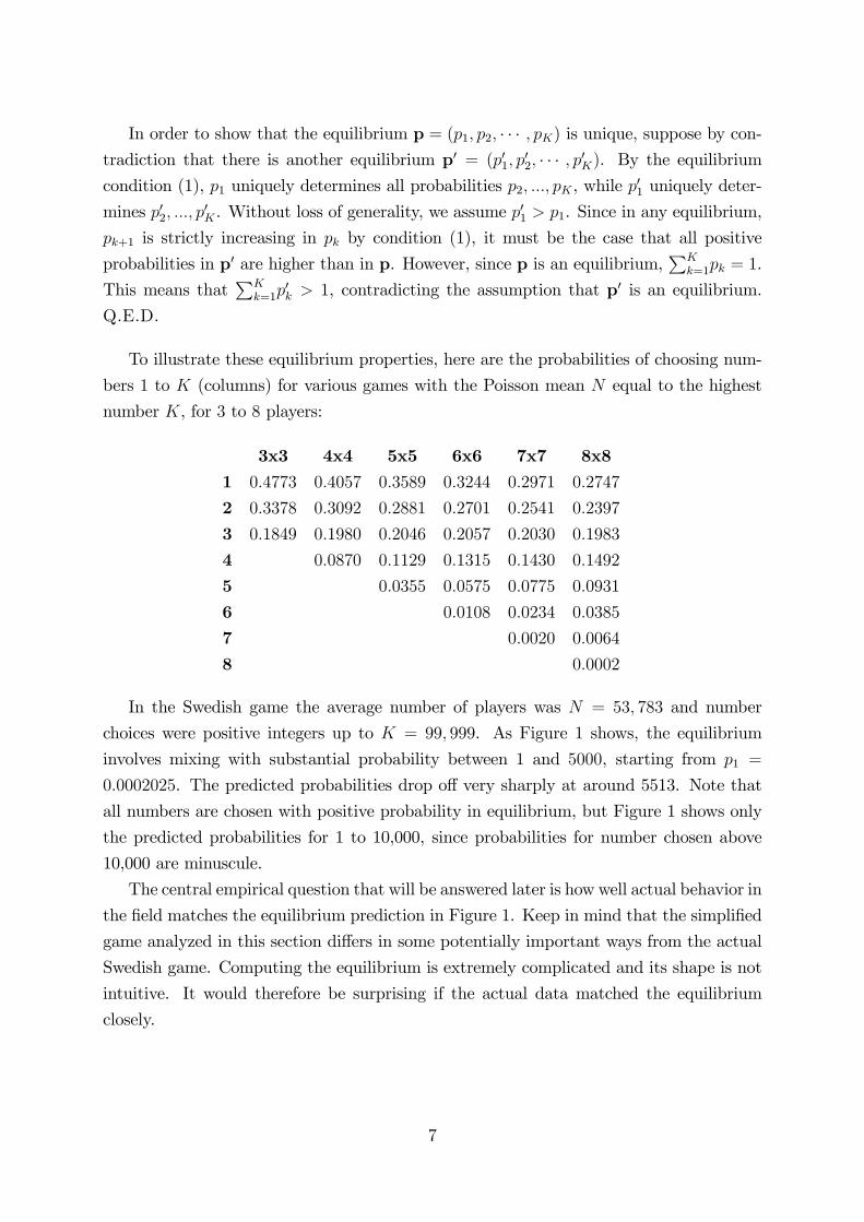
To illustrate these equilibrium properties, here are the probabilities of choosing num-

bers 1 to K (columns) for various games with the Poisson mean N equal to the highest

number K, for 3 to 8 players:

3x3 4x4 5x5 6x6 7x7 8x81 0:4773 0:4057 0:3589 0:3244 0:2971 0:2747

2 0:3378 0:3092 0:2881 0:2701 0:2541 0:2397

3 0:1849 0:1980 0:2046 0:2057 0:2030 0:1983

4 0:0870 0:1129 0:1315 0:1430 0:1492

5 0:0355 0:0575 0:0775 0:0931

6 0:0108 0:0234 0:0385

7 0:0020 0:0064

8 0:0002

In the Swedish game the average number of players was N = 53; 783 and number

choices were positive integers up to K = 99; 999. As Figure 1 shows, the equilibrium

involves mixing with substantial probability between 1 and 5000, starting from p1 =

0:0002025. The predicted probabilities drop o¤ very sharply at around 5513. Note that

all numbers are chosen with positive probability in equilibrium, but Figure 1 shows only

the predicted probabilities for 1 to 10,000, since probabilities for number chosen above

10,000 are minuscule.

The central empirical question that will be answered later is how well actual behavior in

the �eld matches the equilibrium prediction in Figure 1. Keep in mind that the simpli�ed

game analyzed in this section di¤ers in some potentially important ways from the actual

Swedish game. Computing the equilibrium is extremely complicated and its shape is not

intuitive. It would therefore be surprising if the actual data matched the equilibrium

closely.

7

2.3 Logit QRE

As described in McKelvey and Palfrey (1995) and Chen, Friedman, and Thisse (1997),

the quantal response equilibrium (QRE) replaces best responses by quantal responses,

allowing for either error in actions or uncertainty about payo¤s. In a logit QRE, a vector

p = (p1; p2; � � � ; pK) is a symmetric equilibrium if all probabilities satisfy

pk =exp (��(k))PKj=1 exp (��(j))

;

where payo¤s are expected payo¤s given the equilibrium probabilities.

If we assume that the number of players are Poisson distributed, we can use the

expression for the payo¤ from playing the kth number from the previous section. This

gives the following symmetric QRE probabilities of the game:

pk =exp

��Qk�1i=1 [1� npie�npi ] e�npk

�PK

j=1 exp��Qj�1i=1 [1� npie�npi ] e�npj

� :Note that in a logit QRE, as in the Poisson equilibrium, all numbers are played with

positive probability.

The ratio between pk+1 and pk is

pk+1pk

=exp

��Qki=1 [1� npie�npi ] e�npk+1

�exp

��Qk�1i=1 [1� npie�npi ] e�npk

�= exp

�k�1Yi=1

�1� npie�npi

� ��1� npke�npk

�e�npk+1 � e�npk

�!:

In the logit QRE, the equilibrium probabilities satisfy pk � pk+1 with strict inequality

whenever � > 0 (when � = 0 all strategies are played with equal probability 1=K).8

8To see why this is the case, suppose by contradiction that pk+1 > pk, i.e., pk+1=pk > 1. From theexpression for the ratio pk+1=pk we know that this implies that

�k�1Yi=1

�1� npie�npi

� ��1� npke�npk

�e�npk+1 � e�npk

�!> 0:

Dividing by � (assuming that � > 0) and the multiplicative operator and rearranging we get�1� npke�npk

�enpk > enpk+1 :

Taking logarithms1

nln�1� npke�npk

�> pk+1 � pk:

8

Some intuition about how QRE behaves9 can be obtained from the case implemented

in the lab experiments, which has an average of N = 26:9 players (Poisson-distributed)

and numbers from 1 to K = 99. Figure 2 shows the QRE probability distributions for

three values of � and for the Poisson-Nash equilibrium. When � is low, the distribution

is approximately uniform. As � increases more probability is placed on lower numbers 1-

10. When � is high enough the QRE closely approximates the Poisson-Nash equilibrium,

which puts roughly linear declining weight on numbers 1 to 15 and in�nitesimal weight

on higher numbers.

2.4 Cognitive Hierarchy with Quantal Response

A natural way to model limits on strategic thinking is by assuming that di¤erent players

carry out di¤erent numbers of steps of iterated strategic thinking in a cognitive hierarchy

(CH). This idea has been developed in behavioral game theory by several authors (e.g.,

Nagel, 1995, Stahl and Wilson, 1995, Costa-Gomes, Crawford, and Broseta, 2001 and

Camerer, Ho, and Chong, 2004) applied to many games of di¤erent structures (Camerer,

Ho, and Chong, 2004). A precursor to these models was the insight, developed much

earlier in the 1980�s by researchers studying negotiation, that people often �ignore the

cognitions of others� in asymmetric-information bidding and negotiation games (Bazer-

man, Curhan, Moore, and Valley, 2000).

These models require a speci�cation of how k-step players behave and the proportions

of players for various k. We follow Camerer, Ho, and Chong (2004) and assume that the

proportion of players that do k thinking steps is Poisson distributed with mean � , i.e.,

the proportion of players that think in k steps is given by

f (k) = e��� k=k!:

We assume that k-step thinkers correctly guess the proportions of players doing 0 to k�1steps. Then the conditional density function for the belief of a k-step thinker about the

proportion of l < k step thinkers is

gk (l) =f (l)Pk�1h=0 f (h)

:

The IA and EE properties of Poisson games imply that the number of players that a

Since pk+1 > pk, the right hand side is positive. The left hand side, however, is always negative since1 � npke�npk = P (X (k) 6= 1) (which is a probability between zero and one). This is a contradiction,and we can therefore conclude that pk > pk+1 whenever � > 0.

9We have not shown that the symmetric logit QRE is unique, but no other symmetric equilibria haveemerged during numerical calculations.

9

k-step thinker believes will play strategy i is Poisson distributed with mean

nqki = n

k�1Xj=0

gk (j) pji .

Hence, the expected payo¤ for a k-step thinker of choosing number i is

�k(i) =i�1Yj=1

h1� nqkj e�nq

kj

i� e�nqki :

To �t the data well, it is necessary to assume that players respond stochastically (as in

QRE) rather than always choose best responses (see also Camerer, Palfrey, and Rogers,

2006).10 We assume that level 0 players randomize uniformly across all numbers 1 to K,

and higher-step players best respond with probabilities determined by a power function.11

The probability that a k step player plays number i is given by

pki =

�Qi�1j=1

h1� nqkj e�nq

kj

ie�nq

ki

��PK

l=1

�Qi�1j=1

h1� nqkj e�nq

kj

ie�nql

�� ;for � > 0. In order for probabilities to be increasing in the payo¤ of a number, the

payo¤s have to be non-negative, which is the case in the LUPI game. Since qkj is de-

�ned recursively� it only depends of what lower step thinkers do� it is straightforward

to compute the outcome numerically. Apart from the number of players and the numbers

of strategies, there are two parameters: the average number of thinking steps, � , and the

precision parameter, �.

To illustrate how the CH model behaves, consider the parameters of our lab experi-

ments, in which N = 26:9 and K = 99, with � = 1:5 and � = 2. Figure 3 shows how 0 to

5 step thinkers play LUPI and the predicted aggregate frequency, summing across the dif-

ferent thinking step distributions. In this example, one-step thinkers put most probability

10The reason why quantal response is empirically helpful is that best-response models pile up predictedresponses at a very small range of the lowest integers, which does not match the data when the numberrange is large. That is, if k-step thinkers choose best responses and there are many players, a one-stepthinker always chooses 1. A two-step thinker anticipates that others will randomize or choose 1, so shechooses 2. In games where the number range is large, this best-response CH approach predicts numberchoices will be highly clustered at only the �rst few integers. Assuming quantal response smoothes outthe predicted choices over a wider number range.11A logit choice function �ts substantially worse in this case. Note that the logit form implies invariance

of choice probabilities to adding a constant to all payo¤s, while the power form implies invariance tomultiplying payo¤s by a positive number. The fact that selected and unselected players in the labexperiment playing for money and pride, respectively, behave similarly is consistent with the powerfunction implication that changing stake in scale does not matter much, assuming that there is someintrinsic payo¤ even when there is no money payo¤.

10

on number 1, whereas two-step thinkers put most probability on number 5. Three-step

thinkers put most probability on numbers 3 and 7. (Remarkably, these predictions put

more overall weight on odd numbers, which is evident in the �eld data too.)

Figure 4 shows the prediction of the cognitive hierarchy model for the parameters of the

�eld LUPI game, i.e., when N = 53; 783 and K = 99; 999. The dashed line corresponds

to the case when players do relatively few steps of reasoning and their responses are very

noisy (� = 3 and � = 0:008). The dotted line corresponds to the case when players do

more steps of reasoning and respond more precisely (� = 10 and � = 0:011).

There is an important contrast between the ways in which QRE and CHmodels deviate

from equilibrium. QRE predicts number choices will be more evenly spread across the

entire range than what equilibrium predicts; i.e., there will be too few low numbers and

too many higher numbers. As Figure 4 shows, when compared to Poisson equilibrium,

CH predicts there will be too many very low numbers, not enough numbers at the high

end (e.g. 3000 to 5518 in Figure 4, when � and � are low, and 4500 to 5518 when � and

� are high).

3 The Field LUPI Game

The �eld version of LUPI called Limbo, was introduced by the Swedish government-owned

gambling monopoly Svenska Spel on the 29th of January 2007.12 This section describes

its essential elements with additional description in Appendix C.

In Limbo, players chose up to six integers between 1 and 99,999, and each number bet

costs 10 SEK each (approximately 1 EURO). The game was played daily and the winning

number was presented on TV in the evening and on the Internet. The winner received

18 percent of the total sum of bets, with the prize guaranteed to be at least 100,000 SEK

(approximately 10,000 EURO).13 In the unlikely event that there is no number that only

one player picked, which never happened, the prize would have been split between those

who chose the lowest number with the fewest number of bets. There were also second

and third prizes, as well as a special weekly ��nal prize�. The second prize was 1000 SEK

and was received by everyone who chose numbers that were close (below or above) to the

winning number. The third prize was 20 SEK and was received by everyone who chose

numbers close to the winning number, but not close enough to win the second prize.14

12Stefan Molin at Svenska Spel told us that he invented the game in 2001 after taking a game theorycourse from the Swedish theorist and experimenter Martin Dufwenberg.13The prize guarantee of 100,000 SEK was �rst extended until the 11th of March and then to the 18th

of March. We use data from the 29th of January to the 18th of March, so the prize guarantee coveredall days for which we have data.14The thresholds for the second and third prizes were determined so that the second prizes constituted

11

The winner of the �rst prize also won the possibility to participate in a ��nal game�.15

The �nal game ran weekly and had four to seven participants. The ��nal game�consisted

of three rounds where the participants chose two numbers in each round. The rules of

this game were very similar to the original game, but what happened in this game did not

depend on what number you chose in the main game, so we leave out the details about

this game.

During the �rst three to four weeks, it was only possible to play the game at physical

branches of Svenska Spel. Players had to �ll out the form shown in Figure A1 when

playing at physical branches. The form allowed players to bet on up to six numbers,

and it also allowed players to play the same numbers for up to 7 days in a row. More

importantly, there was also an option called �HuxFlux�, which indicated that the player

wanted a computer to select a number. The computer selected numbers from a uniform

distribution where the support of the distribution was determined by the play during the

7 previous days.16 It became possible to play the game on the Internet sometime between

the 21st and 26th of February 2007. The web interface for online play is shown in Figure

A2. This interface also included the option �HuxFlux�, but in this case players could see

the number that was generated by the computer before deciding whether to place the bet.

We use daily data from the �rst seven weeks. The reason is that the game was

withdrawn from the market on the 24th of March 2007 and we were only able to access

data up to the 18th of March 2007. The game was stopped one day after a newspaper

article claimed that some players had colluded in the game, but it is unclear to what extent

collusion actually occurred.17 Unfortunately, we have only gained access to aggregate daily

frequencies, not to individual data. The data used includes choices from players that let

a random number generator pick an integer for them.18

Note that the theoretical analysis of the LUPI game di¤ers from the �eld LUPI game

11 percent of all bets and the third prizes 17.5 percent.153.5 percent of all daily bets were reserved for this ��nal game�.16In the �rst week HuxFlux randomized numbers uniformly between 1 and 15000. After seven days of

play, the computer randomized uniformly between 1 and the average 90th percentile from the previousseven days. However, the only information given to players about HuxFlux was that a computer wouldchoose a number for them.17The rule that players could only pick up to six numbers a day was enforced by the requirement that

players had to use a �gambler�s card� linked to their personal identi�cation number when they played.Colluding in LUPI can increase the probability of winning. For example, in the �eld data we obtained,the lowest number not played was always below 4800, meaning that a coalition consisting 800 peopleeach choosing 6 distinctive numbers could guarantee a win facing the empirical distribution of bets inany given day. The total payo¤ for the coalition would be at least 100; 000 � 48; 000 = 52; 000 (SEK).Note this requires a large number of people to work, and will fail miserably if more than one coalitionact on the same day.18We don�t know exactly how many players used this option. However, in the �rst week, we can infer

that the number of players choosing this option was approximately 19 percent. (Since we know the uppercuto¤ for the randomizing device, we use the number of bets above and below this cuto¤ to get thisapproximation.)

12

in three respects. First, in the theoretical analysis we assume a tie-breaking rule such

that nobody gets anything if there is no unique number. In the �eld version of LUPI, the

prize is split between those that guessed the lowest number with the fewest number of

guesses. Since the probability that there is no number that only one player guessed is very

small when the number of players and numbers to choose from are large, we believe that

this di¤erence plays little role for the theoretical predictions. A second, more important,

di¤erence is that we assume that each player can only pick one number. In the �eld

game, players are allowed to bet on up to six numbers. This does play a role for the

theoretical predictions, since it allows players to �knock out�a winner by choosing the

same number twice and then bet on a higher number hoping that this will be the only

winning number. However, this di¤erence is less likely to play a role when the number of

players is very large, as it is in our �eld data. Finally, we do not take the second and third

prizes present in the �eld version into account, but this is unlikely to make a big di¤erence

for the strategic nature of the game. Nevertheless, these three di¤erences between the

game analyzed theoretically and the �eld game is an important motivation for why we

also run laboratory experiments with single bets, no opportunity for direct collusion, and

only a �rst prize, which match the game analyzed theoretically.

3.1 Descriptive Statistics

Table 1 reports summary statistics for the �rst 49 days of the game. To get some notion

of possible learning over time, two additional columns display the corresponding daily

averages for the �rst and last weeks. The last column displays the corresponding statistics

that would result if players played according to Poisson-Nash equilibrium.

Overall, the average number of bets was 53,783, but there was considerable variation

over time. There is no apparent time trend in the number of participating players, but

there is less participation on Sundays and Mondays (see Figure A3). The variation of the

number of bets across days is therefore much higher than what the Poisson distribution

predicts (its standard deviation is 232), which is one more reason to expect the equilibrium

prediction to not �t very well.

However, the average number chosen overall was 2835, which is close to the equilibrium

prediction of 2595. Winning numbers, and the lowest numbers not chosen by anyone, also

varied a lot over time. Comparing the �rst and last week, all the aggregate statistics

and frequencies in low-number intervals converge reasonably closely to equilibrium. For

example, in equilibrium essentially nobody should choose a number above 10,000. In the

�rst week 12 percent chose these high numbers, but that fraction fell to one percent in

the last week.

13

All days 1st week 7th week Eq.Avg. Std. Min Max Avg. Avg. Avg.

# Bets 53783 7782 38933 69830 57017 47907 53783Average number played 2835 813 2168 6752 4512 2484 2595Median number played 1674 348 435 2272 1203 1935 2541Winning number 2095 1266 162 4465 1159 1982 2585Lowest number not played 3103 929 480 4597 1745 3462 4077Below 100 (%) 6.08 4.84 2.72 2.97 15.16 3.19 2.02Below 1000 (%) 32.31 8.14 21.68 63.32 44.91 27.52 20.05Below 5000 (%) 92.52 6.44 68.26 97.74 78.75 96.44 93.34Below 10000 (%) 96.63 3.80 80.70 98.94 88.07 98.81 100.00Even numbers (%) 46.75 0.58 45.05 48.06 45.91 47.45 49.99Divisible by 10 (%) 8.54 0.466 7.61 9.81 8.43 9.01 9.99Proportion 1900�2010 (%) 71.61 4.28 67.33 87.01 7.94 68.79 49.7811, 22, etc. (%) 12.2 0.82 10.8 14.4 12.4 11.4 9.00111, 222 etc. (%) 3.48 0.65 2.48 4.70 4.27 2.78 0.901111, 2222, etc. (�) 4.52 0.73 2.81 5.80 4.74 3.95 0.7411111, 22222, etc. (�) 0.76 0.84 0.15 5.45 2.26 0.21 0

Proportion of numbers between 1900 and 2010 refers to the proportion relative to numbers between1844 and 2066. "11, 22, etc" refers to the proportion relative to numbers below 100, "111,222, etc"relative to numbers below 1000 and so on. The prediction refers to the equilibrium with n = 53; 783 andK = 99; 999:

Table 1: Descriptive statistics for �eld data

An interesting feature of the data is a tendency to avoid round or focal numbers and

choose quirky numbers that are perceived as �anti-focal�(as in hide-and-seek games, see

Crawford and Iriberri, 2007). Even numbers were chosen less often than odd ones (46.75%

vs. 53.25%). Numbers divisible by 10 are chosen a little less often than predicted. Strings

of repeating digits (like 1111) are chosen too often.19 Players also overchoose numbers that

represent years in modern time (perhaps their birth years), except for round years (e.g.,

1950). If players had played according to equilibrium, the fraction of numbers between

1900 and 2010 divided by all numbers between 1844 and 2066 should be 49.78 percent,

but the actual fraction was 70 percent. Figure 5 shows a histogram of numbers between

1900 and 2010 (aggregating all 49 days). Note that although the numbers around 1950

are most popular, there are dips at years that are divisible by ten. Figure 5 also shows

the aggregate distribution of numbers between 1550 and 2400, which clearly shows the

popularity of numbers around 1950 and 2007. There are also spikes in the data for special

19Similar behavior can be found in the federal tax evasion case of Joe Francis, the founder of �GirlsGone Wild.�Mr. Francis was indicted on April 11, 2007 for claiming false business expenses such as$333,333.33 and $1,666,666.67 in insurance, which were too suspicious not to attract attention. Seehttp://consumerist.com/consumer/taxes/girls-gone-wild-tax-indictment-teaches-us-not-to-deduct-funny+looking-numbers-252097.php for the proposed tax lesson.

14

numbers like 2121, 2222 and 2345.

3.2 Results

Do subjects in the �eld LUPI game play according to the equilibrium prediction? In order

to investigate this, we assume that the number of players is Poisson distributed with mean

equal to the empirical daily average number of numbers chosen (53783). As noted, this

assumption is wrong because the variation in number of bets across days is much higher

than what the Poisson distribution predicts.

Recall that in the Poisson equilibrium, probabilities of choosing higher numbers �rst

decrease slowly, drop quite sharply at around 5500, and asymptotes to zero after p5513 �1=n (recall Proposition 1 and Figure 1). Figure 6 shows the average daily frequencies from

the �rst week together with the equilibrium prediction (indicated by the dashed line), for

all numbers up to 100,000 and for the restricted interval up to 10,000. Compared to

equilibrium, there is overshooting at numbers below 1000 and undershooting at numbers

between between 2000 and 5500. It is also noteworthy how spiky the data is compared

to the equilibrium prediction, which is a re�ection of clustering on special numbers, as

described above.

Figure 7 shows average daily frequencies of choices from the second through the last

(7th) week. Behavior in this period is much closer to equilibrium than in the �rst week.

Indeed, when the full range of numbers is graphed (the left-hand graph) it is clear that

there are too many low choices, but the frequencies do drop o¤ sharply quite close to

where the equilibrium predicts a dropo¤. However, when only numbers below 10,000 are

plotted, the overshooting of low numbers and undershooting of intermediate numbers is

still clear and there are still many spikes of clustered choices. (These two deviations are

still evident even in the seventh and last week, as shown in Figure A4.)

Statistical tests of the signi�cance of these deviations are unnecessary because the large

sample sizes will reject the equilibrium hypothesis strongly. The more important question

is whether alternative theories can explain both the degree to which the equilibrium

prediction is surprisingly accurate and the degree to which there is systematic deviation.

3.3 Rationalizing Non-Equilibrium Play

In this section, we investigate if the cognitive hierarchy model can account for the two main

deviations from equilibrium just described in the previous section. We do not estimate

the QRE model because it cannot account for overshooting of low numbers, and it is very

15

computationally challenging to estimate for the large-scale �eld data. (We do estimate it

for the lab data discussed later.)

Table 2 reports the results from the maximum likelihood estimation of the data using

the cognitive hierarchy model.20 The best-�tting estimates week-by-week, shown in Table

2, suggest that both parameters increase over time. The average number of thinking steps

that people carry out, � , increases from about 3 in the �rst week� an estimate reasonably

close to estimates from 1.5 to 2.5 that typical �t experimental data sets well (Camerer,

Ho, and Chong, 2004) to 10 in the last week.

Week 1 2 3 4 5 6 7� 2.9777 5.8338 7.3156 7.208 7.8175 10.2672 10.2672� 0.0080 0.0094 0.0103 0.0108 0.0110 0.0108 0.0107

Table 2: Maximum likelihood estimation of the cognitive hierarchy model for �eld data

Figure 8 shows the average daily frequencies from the �rst week together with the

cognitive hierarchy estimation and equilibrium prediction. The cognitive hierarchy model

does a reasonable job of accounting for the over- and undershooting tendencies at low and

intermediate numbers. The model also accounts for the fact that some players pick very

high numbers (which any model with extra randomness will do). For the �rst week, the

cognitive hierarchy model predicts that 5 percent of all numbers are above 10,000, which

is too low since the corresponding number in data from the �rst week is 12 percent, but is

closer than the equilibrium prediction of approximately zero. Furthermore, while the CH

model does have two degrees of freedom which the Poisson equilibrium prediction does

not, there is a large amount of data so the good account of the deviations is not due to

over�tting.

In the last week, the estimated � and � both are considerably higher. As a result,

the cognitive hierarchy prediction is much closer to equilibrium but still accounts for the

smaller over- and undershooting (see Figure 9).

To get some notion of how close to the data the �tted cognitive hierarchy model is,

Table 3 displays two goodness-of-�t statistics. The log-likelihoods reveal that the cognitive

hierarchy model does better in explaining the data toward the last week. (Likelihoods of

the Poisson-Nash equilibrium are an unfair test because many numbers are chosen that

have essentially zero predicted probability; likelihood comparisons like the Vuong test

would therefore very strongly reject the equilibrium prediction.)

In order to compare the CH model with the equilibrium prediction, we calculate the

20It is di¢ cult to guarantee that these estimates are global maxima since the likelihood function isnot smooth and concave. We also used a relatively coarse grid search, so there may be other parametervalues that yield higher likelihoods.

16

proportion of the empirical density that lies below the predicted density, i.e., the propor-

tion of choices that were correctly predicted. This statistic also shows that the cognitive

hierarchy model can explain the data better toward the end of the time period. The

cognitive hierarchy model does better than the equilibrium prediction in all seven weeks

based on this statistic. For example, in the �rst week, 61 percent of players�choices were

consistent with the cognitive hierarchy model, whereas only 50 percent were consistent

with equilibrium. However, the cognitive hierarchy model is �tted with two free para-

meters, whereas the equilibrium prediction is calculated without any parameters. We

therefore can not conclude that one of the two models is better.

Week 1 2 3 4 5 6 7Log-likelihood CH -63956 -36390 -23716 -20546 -20255 -19748 -18083Proportion below CH (%) 61.08 72.50 77.69 79.87 81.86 82.63 81.94Proportion below eq. (%) 49.56 61.82 67.66 67.70 70.23 76.79 76.61

The proportion below the theoretical prediction refers to the fraction of the empirical density thatlies below the theoretical prediction.

Table 3: Goodness-of-�t for cognitive hierarchy and equilibrium for �eld data

The players� tendency to embrace or avoid particular numbers is more di¢ cult to

explain using general formal models. As was shown in Table 1, players seem to have pref-

erences for odd numbers, numbers that represent round-numbered years, and repeating

same-digit strings, whereas they avoid numbers divisible by 10 and even numbers. In

the CH approach, the natural way to model this is to assume that 0-step thinkers do

not choose randomly, but they instead choose using simple low-e¤ort heuristics, including

prominent numbers. One-step thinkers then correctly avoid these numbers and choose

anti-focal numbers (e.g. avoiding numbers that are multiples of 10). It is hard to explain

these choices parametrically without some theory of what makes certain choices focal or

anti-focal, so we simply note this tendency and leave a deeper understanding to future

research. Note however that Crawford and Iriberri (2007) use a CH approach to explain

similar patterns in simpler hide-and-seek games. In their games the number of strategies

is small, so the strategies which are not focal (in a graphical display) are typically anti-

focal. With the large number of strategies in our games the same approach does not work

so neatly (e.g., avoid the numbers 10 and 20 do not necessarily point to the choices of 11

and 22, neither than 16 or 28).

17

4 The Laboratory LUPI Game

The rules of the �eld LUPI game do not exactly match the theoretical assumptions used

to generate the predicted equilibrium described above. The �eld data included some

choices made by a random number generator and some players might have chosen mul-

tiple numbers or simply colluded. It is possible that these features can account for the

discrepancies between the data and the equilibrium prediction. We then took the natural

next step, playing the LUPI game in a controlled laboratory environment which more

closely matches the assumptions of the theory.

In designing the laboratory game, we compromise between two goals: to create a

simple environment in which theory should apply (theoretical validity), and to recreate

the features of the �eld LUPI game in the lab. Because we use this opportunity to

create an experimental protocol that is closely matched to a particular �eld setting, we

sometimes sacri�ced theoretical validity for �eld replication.

The �rst choice is the scale of the game, in number of players (N), permissible numbers

(K), and stakes. We choose to scale down the number of players and the largest payo¤

by a factor of roughly 2000. This implies that there were on average of 26.9 players and

the prize to the winner in each round was $7, whereas we used K = 99.21 Since the

�eld data span 49 days, the experiment has 49 rounds in each session. (We typically

refer to experimental rounds as �days�and seven-�day�intervals as �weeks�for semantic

comparability between the lab and �eld descriptions.) While the winning number was

announced in each �eld-game day, we do not know how much subjects learned about the

number distribution (which was only available online); thus, we choose to announce only

the winning number in the lab.

Because the number of players is endogenous in the �eld, in the lab experiment the

number of players in each round was also determined randomly. In two sessions, we scaled

down the empirical distribution of number of bets in the �eld as in the 49 days by 2000,

then re-scaled it so that the mean equals the variance (both are 26.9), consistent with

a Poisson distribution. In a third session, we used a Poisson distribution with a mean

of 26.9 players to generate the numbers of players. Because players in the �eld did not

necessarily know the number of players, we did not tell the lab subjects the process by

which the number of players in each round was determined. This is an example of how

the design opted for lab-�eld parallelism at the expense of theoretical validity.

In contrast to the �eld game, each player was allowed to choose only one number and

there was only one prize per round, in the amount of $7. There was no option to use

21Rescaling by 2000 would lead to a range from 1 to K = 50, but we used K = 99 since we worriedthat we otherwise would miss the chance to see some focal numbers like 66 and 88.

18

a random number generator and in the case there was no number that only one player

picked, nobody won in that round. These rules implement theoretical assumptions but

depart from the rules in the �eld game.

Three laboratory sessions were conducted at the California Social Science Experi-

mental Laboratory (CASSEL) at University of California Los Angeles on the 22nd and

25th of March 2007. The experiments were conducted using the Zürich Toolbox for

Ready-made Economic Experiments (zTree) developed by Urs Fischbacher, as described

in Fischbacher (2007). Within each session, 38 graduate and undergraduate students were

recruited, through CASSEL�s web-based recruiting system, to participate. All subjects

had the knowledge that their payo¤ will be determined by their performance. We made

no attempt to replicate the demographics of the �eld data, which we unfortunately know

very little about. However, the players in the laboratory are likely to di¤er in terms of

gender, age and ethnicity compared to the Swedish players. In all three sessions, we had

more female than male subjects, with all of them clustered in the age bracket of 18 to

22, and the majority spoke a second language. The majority of the subjects had never

participated in any form of lottery before. According to subjects�self-perceived income

group, roughly half indicated that they were below the 50th percentile.22 Subjects had

various levels of exposure to game theory, but very few had seen or heard of a similar

game prior to this experiment.

4.1 Experimental Procedure

At the beginning of each session, the experimenter �rst explained the rules of the LUPI

game. The instructions were based on a version of the lottery ticket for the �eld game

translated from Swedish to English (see Appendix D). Subjects were then given the option

of leaving the experiment, in order to see how much self-selection in�uences experimental

generalizability. None of the recruited subjects chose to leave, which indicates a limited

role for self-selection (after recruitment and instruction).

After having received everyone�s consent, the experiment continued. In order to avoid

an end-game e¤ect, subjects were told that the experiment would end at a predeter-

mined, but non-disclosed time (also matching the �eld setting, which ended abruptly and

unexpectedly). Subjects were told that participation was randomly determined at the

beginning of each round, with 26.9 subjects participating on average. In the beginning of

each round, subjects were informed whether they would participate in the current round.

22Subjects were asked to report their household income percentile. Since we were interested in howthe subjects perceived themselves, we purposely did not de�ne the size of household, whether countingthemselves as independent head of household or as a dependent of their parents�household. Along thesame line of reasoning, we did not provide subjects with the current national income distribution.

19

They were required to submit a number in each round, even if they were not selected to

participate. (The di¤erence between behavior of selected and non-selected players gives

us some information about the e¤ect of marginal incentives.)

When all subjects had submitted numbers, the lowest unique positive integer was

determined. If there was a lowest unique positive integer, the winner earned $7. Each

subject was privately informed, immediately after each round, what the winning number

was, whether they had won that particular round, and their payo¤ so far during the

experiment. This procedure was repeated 49 times, with no practice rounds (as is the case

of the �eld). After the last round, subjects were asked to complete a short questionnaire

which allowed us to build the demographics of our subjects and a classi�cation of strategies

used. In one of the sessions, we included the cognitive re�ection test as a way to measure

cognitive ability (to be described below). All sessions lasted for less than an hour, and

subjects received a show-up fee of $8 or $13 in addition to prizes from the experiment

(which averaged $8.6).

Screenshots from the experiment are shown in Appendix D.

4.2 Lab Descriptive Statistics

Behavior in the laboratory di¤ers slightly among the three sessions. We cannot reject

that the two sessions that used the scaled down �eld distribution of number of players are

di¤erent (the p-value using a Mann-Whitney test is 0:44), but the session that follows an

actual Poisson distribution is statistically di¤erent from the pooled data from the other

two sessions (Mann-Whitney p-value 0:009). However, if we only use the choices of players

who were selected to participate in each round, we cannot reject that the distribution of

the data is the same in all sessions at p < 0:05.23

In the remainder of the paper, we therefore pool the data from all three sessions, but

only use the choices of participating subjects. It should be noted, however, that we cannot

reject that participating and non-participating players�behavior di¤er when pooling data

from all sessions (Mann-Whitney p-value 0:16). Figure 10 displays the aggregate data

from non-selected and selected subjects�choices. Subjects are slightly more likely to play

high numbers above 20 when they are not selected to participate, but overall the pattern

looks very similar. This implies that subjects�behavior in a particular round is almost

una¤ected depending on whether they had marginal monetary incentives or not.

23Using only selected players�choices, a Mann-Whitney test of the null hypothesis that the two sessionswith the �eld distribution are the same results in a p-value of 0.22. Separately comparing the Poissonsession with the two sessions with the �eld distribution of players result in p-values of 0.06 and 0.46.Comparing the session with the Poisson distribution with the pooled data from the two sessions with the�eld distribution results in a p-value of 0.13.

20

Figure 11 shows the data for the choices of participating players. There are very few

numbers above 20 and we therefore focus on the numbers 1 to 20 in the following graphs.

In line with the �eld data, players have a predilection for certain numbers, while others

are avoided. Judging from Figure 11, subjects avoid some even numbers, especially 2 and

10, while they endorse the odd (and prime) numbers 3, 11, 13 and 17. Interestingly, no

subject played 20, while 19 was played �ve times and 21 was played six times.

All rounds R 1-7 R. 43�49 Eq.Avg. Std.dev. Min Max Avg. Avg. Avg.

Average number played 5.7 1.6 4.2 13.1 9.0 5.3 5.2Median number played 4.8 1.0 3.5 8.0 6.0 5.0 5Below 20 (%) 98.13 3.43 78.05 100.00 92.81 98.83 1.00Even numbers (%) 44.07 5.84 29.47 56.94 39.79 47.16 46.86Session 1 (Field dist.)Winning number 6.0 9.3 1 67 13.0 2.5 2.9Lowest number not played 8.1 2.5 1 12 4.9 8.1 3.3Session 2 (Poisson dist.)Winning number 5.1 2.6 1 10 5.8 5.1 2.9Lowest number not played 7.5 2.9 1 12 6.3 8.4 3.3Session 3 (Field dist.)Winning number 5.6 3.2 1 14 6.1 5.7 2.9Lowest number not played 7.5 2.7 2 13 7.4 10.0 3.3

Summary statistics are based only on choices of subjects that are selected to participate. Theequilibrium column refers to what would result if all players played according to equilibrium (n = 26:9and K = 99)

Table 4: Descriptive statistics for laboratory data

Table 4 shows some descriptive statistics for the participating subjects in the lab

experiment. As in the �eld, some players in the �rst week tend to pick very high numbers.

In the �rst week, 93 percent of all numbers are below 20 (7 percent above 20), while only

one percent chose above 20 in the last week. The average number chosen in the last

week corresponds closely to the equilibrium prediction (5.3 vs. 5.2) and the medians are

identical (5.0). The average winning numbers are too high compared to equilibrium play,

which is consistent with the observation that players pick very low numbers too much,

creating non-uniqueness among those numbers so that unique numbers are high. The

tendency to pick odd numbers decreases over time� 40 percent of all numbers are even

in the �rst week, whereas 47 percent are even in the last week (which coincides with the

equilibrium proportion of even numbers).

21

4.3 Aggregate Results

In the Poisson equilibrium with 26.9 average number of players, strictly positive prob-

ability is put on numbers 1 to 16, while other numbers have probabilities numerically

indistinguishable from zero. Figure 12 shows the average frequencies played in week 1 to

7 together with the equilibrium prediction (dashed line) and the estimated week-by-week

results using the cognitive hierarchy model (solid line). These graphs clearly indicates

that learning is quicker in the laboratory than in the �eld. Despite that the only feedback

given to players in each round is the winning number, behavior is remarkably close to equi-

librium already in the second week. However, we can also observe the same discrepancies

between the equilibrium prediction and observed behavior as in the �eld. The distribution

of numbers is too spiky and there is overshooting of low numbers and undershooting at

numbers just below the equilibrium cuto¤.

Figure 12 also displays the estimates from a maximum likelihood estimation of the

cognitive hierarchy model presented in the theoretical section (solid line). The cognitive

hierarchy model can account both for the spikes and the over- and undershooting. Table

5 shows the estimated parameters.24 There is no clear time trend in the two parameters,

and in some rounds the average number of thinking steps is unreasonably large compared

to other experiments showing � around 1.5. Since there are two free parameters with

relatively few choice probabilities to estimate, we might be over-�tting by allowing two

free parameters. We therefore estimate the precision parameter � while keeping the

average number of thinking steps �xed. We set the average number of thinking steps to

1:5, which has been shown to be a value of � that predicts experimental data well in a large

number of games (Camerer, Ho, and Chong, 2004). The estimated precision parameter

is considerably lower in the �rst week, but is then relatively constant. Figure 13 shows

the �tted cognitive hierarchy model when � is restricted to 1:5. It is clear that the model

with � = 1:5 can account for the undershooting also when the number of thinking steps

is �xed, but it has di¢ culties in explaining the overshooting of low numbers. The main

problem is that with � = 1:5, there are too many zero-step thinkers that play all numbers

between 1 and 99 with uniform probability.

Table 5 also displays the maximum likelihood estimate of � for the logit QRE. The

precision parameter is relatively high in all weeks, but particularly from the second week

and onwards. Recall from Figure 2 that the QRE prediction for such high � is very close

to the Poisson-Nash equilibrium.

Table 6 provides some goodness-of-�t statistics for the cognitive hierarchy model, QRE

and the equilibrium prediction. The table reveals that the cognitive hierarchy estimations24The log-likelihood function is neither smooth nor concave, so the estimated parameters may not

re�ect a global maximum of the likelihood.

22

Week 1 2 3 4 5 6 7� 8.15 13.14 6.48 5.31 11.52 5.05 9.00� 1.19 11.27 10.85 14.92 13.53 14.67 8.73� (� = 1:5) 1.08 2.37 2.85 2.82 2.76 2.34 2.16�QRE 123.40 526.83 396.24 430.83 523.30 517.25 309.89

Table 5: Maximum likelihood estimation of the cognitive hierarchy model and QRE forlaboratory data

�t the data better after the �rst week. Comparing the proportion of correctly predicted

choices, the equilibrium prediction does remarkably well. The equilibrium prediction does

better than the cognitive hierarchy model with � = 1:5 in all weeks, but the cognitive

hierarchy model with two free parameters does better than the equilibrium prediction in all

but the second week. Allowing for noise, the logit QRE performs better than equilibrium

in the �rst week, but is practically indistinguishable from equilibrium after the �rst week

(due to high �). Since the logit QRE includes the Poisson equilibrium as a special case

(when � ! 1), the log-likelihood of the logit QRE provides an upper bound for thatof the Poisson-Nash equilibrium. Hence, comparing the log-likelihood of logit QRE and

cognitive hierarchy, we also see that the Poisson-Nash equilibrium (using logit QRE as

bound) out-performs the cognitive hierarchy model with � = 1:5, but is out-performed by

the cognitive hierarchy model with two free parameters.

Week 1 2 3 4 5 6 7Log-likelihood CH -150.9 -75.9 -67.5 -65.0 -64.4 -60.7 -68.5Log-likelihood CH � = 1:5 -204.1 -180.8 -171.6 -179.8 -177.8 -178.4 -185.8Log-likelihood logit QRE -172.2 -76.8 -94.8 -88.5 -82.0 -76.9 -88.9Proportion below CH (%) 86.06 88.02 92.26 93.13 91.41 94.99 92.60Proportion below CH � = 1:5 (%) 81.11 76.53 79.00 76.79 78.23 76.22 77.18Proportion below logit QRE (%) 84.95 87.94 83.64 86.88 86.13 90.21 86.61Proportion below eq. (%) 81.71 88.16 83.60 87.19 86.13 90.79 86.88

The proportion below the theoretical prediction refers to the fraction of the empirical density that liesbelow the theoretical prediction.

Table 6: Goodness-of-�t for cognitive hierarchy, QRE and equilibrium for laboratory data

On the aggregate level, behavior in the lab is remarkably close to equilibrium from the

second to the last week. The cognitive hierarchy model can rationalize the tendencies that

some numbers are played more, as well as the undershooting below the equilibrium cuto¤.

The value-added of the cognitive hierarchy model is not primarily that it gives a slightly

better �t, but that it provides a plausible story for how players manage to play so close

to equilibrium. Most likely, few players would be capable of calculating the equilibrium

23

during the course of the experiment, whereas many of them should be able to carry out

a few steps of reasoning along the lines of the cognitive hierarchy model.

4.4 Individual Results

Behavior on the aggregate level is close to equilibrium, which is particularly remarkable

since subjects received very little feedback during the experiment (only the winning num-

bers). In the post-experimental questionnaire, several subjects said that they responded

to previous winning numbers, so we regressed players�choices on the winning number in

previous periods. Table 7 shows that the winning numbers in previous rounds do a¤ect

players�choices early on. In the �rst and second weeks, if the winning number was high,

players tend to choose higher numbers in the next round. However, this tendency is con-

siderably weaker in later weeks 3-7. The small round coe¢ cients in Table 7 also show

that there does not appear to be any general trend in players�choices over the 49 rounds.

All periods Week 1 Week 2 Week 3-7Round (1-49) -0.011 -0.529 -0.102 0.0144

(-1.09) (-0.58) (-0.47) (1.10)t� 1 winner 0:188�� 0:154�� 0:376� 0:089�

(10.55) (3.55) (2.20) (1.98)t� 2 winner 0:140�� 0:111� 0.323 0.056

(7.43) (1.99) (1.28) (1.26)t� 3 winner 0:082�� 0.078 -0.057 0.036

(4.10) (1.13) (-0.26) (0.83)Fixed e¤ects Yes Yes Yes YesObservations 3156 319 483 2354R2 0.05 0.12 0.01 0.00

*=5 percent and **=1 percent signi�cance level. The table reportresults from a linear �xed e¤ects panel regression. Only selectedsubjects are included. t�statistics within parentheses.

Table 7: Panel data regressions explaining individual play in the laboratory

The regression results in Table 7 mask a considerably degree of heterogeneity between

individual subjects. In the post-experimental questionnaire, we asked people to state why

they played as they did. Based on these responses we coded four variables depending on

whether they mentioned each aspect as a motivation for their strategy.

Random All subjects who claimed that they played numbers randomly were coded in

this category.25

25For example, one subject motivated this strategy choice in a particular sophisticated way: �First I

24

Stick All subjects who stated that they stuck to one number throughout parts of theexperiment were included in this category. Many of these subjects explained their

choices by arguing that if they stuck with the same number, they would increase

the probability of winning.

Lucky This category includes all subjects who claimed that they played a favorite orlucky number.

Strategic This category includes all players who explicitly motivated their strategy byreferring to what the other players would do.26

Several subjects were coded into more than one category.27 The fraction of subjects

within each set of categories are reported in Table 8.

(%) Random Stick Lucky StrategicRandom 35.1 7.0 1.8 7.0Stick 34.2 3.5 15.8Lucky 10.5 4.4Strategic 41.2

Table 8: Classi�cation of self-reported strategies

How well does the classi�cation based on the self-reported strategies explain behavior?

Table 9 reports regressions where the dependent variables are four summary statistics of

subjects�behavior� the number of distinct choices, the mean number, the standard devi-

ation of number, and the total payo¤. In the �rst column for each measure of individual

play only the four categories above are included as dummy variables. There are few

statistically signi�cant relationships. Subjects coded into the �Stick�category did tend

to choose fewer numbers, and subjects coded as �Lucky�tend to pick higher and more

highly varied numbers (high standard deviation). Table 9 also report regressions for

the same dependent variables and some demographic variables.28 The only statistically

tried logic, one number up or down, how likely was it that someone else would pick that, etc. That wasn�tdoing any good, as someone else was probably doing the exact same thing. So I started mentally singingscales, and whatever number I was on in my head I typed in. This made it rather random. A couple oftimes I just threw curveballs from nowhere for the hell of it. I didn�t pay any attention to whether ornot I was selected to play that round after the �rst 3 or so.�26For example, one subject stated the following: �I tried to pick numbers that I thought other people

wouldn�t think of� whatever my �rst intuition was, I went against. Then I went against my secondintuition, then picked my number. After awhile, I just used the same # for the entire thing.�27For example, the following subject was classi�ed into all but the �Lucky�category: �At �rst I picked

4 for almost all rounds (stick) because it isn�t considered to be a popular number like 3 and 5 (strategic).Afterwards, I realized that it wasn�t helping so I picked random numbers (random).�28Including demographic variables and the four categories in the same regressions does not a¤ect any

of the results reported here.

25

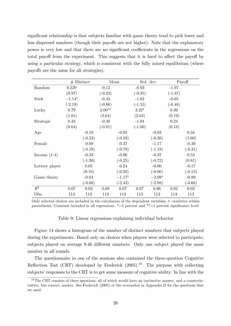
signi�cant relationship is that subjects familiar with game theory tend to pick lower and

less dispersed numbers (though their payo¤s are not higher). Note that the explanatory

power is very low and that there are no signi�cant coe¢ cients in the regressions on the

total payo¤ from the experiment. This suggests that it is hard to a¤ect the payo¤ by

using a particular strategy, which is consistent with the fully mixed equilibrium (where

payo¤s are the same for all strategies).

# Distinct Mean Std. dev. Payo¤Random 0.529 -0.12 -0.93 -1.97

(0.97) (-0.23) (-0.85) (-1.37)Stick �1:14� -0.43 -1.62 -0.65

(-2.19) (-0.86) (-1.55) (-0.48)Lucky 0.79 2:00�� 3:22� 0.39

(1.01) (2.64) (2.04) (0.19)Strategic 0.33 -0.40 -1.04 0.24

(0.64) (-0.81) (-1.00) (0.18)Age -0.19 -0.05 -0.03 0.34

(-0.23) (-0.59) (-0.20) (1.60)Female -0.09 -0.37 -1.17 -0.39

(-0.19) (-0.79) (-1.19) (-0.31)Income (1-4) -0.33 -0.06 -0.37 0.53

(-1.30) (-0.25) (-0.72) (0.81)Lottery player 0.05 -0.24 -0.00 -0.17

(0.10) (-0.50) (-0.00) (-0.13)Game theory -0.04 �1:17� �2:09� -0.89

(-0.08) (-2.43) (-2.08) (-0.68)R2 0.07 0.02 0.08 0.07 0.07 0.06 0.02 0.03Obs. 113 113 113 113 113 113 113 113

Only selected choices are included in the calculation of the dependent variables. t�statistics withinparentheses. Constant included in all regressions. *=5 percent and **=1 percent signi�cance level.

Table 9: Linear regressions explaining individual behavior

Figure 14 shows a histogram of the number of distinct numbers that subjects played

during the experiments. Based only on choices when players were selected to participate,

subjects played on average 9.46 di¤erent numbers. Only one subject played the same

number in all rounds.

The questionnaire in one of the sessions also contained the three-question Cognitive

Re�ection Test (CRT) developed by Frederick (2005).29 The purpose with collecting

subjects�responses to the CRT is to get some measure of cognitive ability. In line with the

29The CRT consists of three questions, all of which would have an instinctive answer, and a counterin-tuitive, but correct, answer. See Frederick (2005) or the screenshot in Appendix D for the questions thatwe used.

26

results reported in Frederick (2005), a majority of the UCLA subjects answered only zero

or one questions correctly. Interestingly, there does not appear to any relation between

player�s behavior or payo¤ in the LUPI game and the number of correctly answered

questions, but the sample size is small (n=38). The number of correctly answered CRT

questions is not signi�cant when the four measures in Table 9 are regressed on the CRT

score.

5 Field vs. Lab

Throughout the history of experimental economics, there has been a simmering debate

about the extent to which laboratory experiments can tell us something about partic-

ular naturally-occurring situations outside the lab (e.g., Loewenstein, 1999). There are

at least two concerns related to this argument. First, to what extent do the often ab-

stract and highly structured games used in laboratory experiments represent phenomena

in �real-world� settings? Second, to what extent do laboratory subjects�behavior dif-

fer from humans in non-laboratory settings, for example because the subject pool is not

representative or due to experimenter e¤ects. In this paper, we address both these con-

cerns. The laboratory experiment in this paper uses the same game� with a few minor

modi�cations� as the game played in the �eld. The lab and �eld LUPI games di¤er, how-

ever, in time, location, context and demographics of the players. In the �eld LUPI game,

players are self-selected from the Swedish population and play with their own money in

a naturally occurring environment. Students at UCLA on the opposite side of the globe

play as experimental subjects in a scrutinized laboratory setting.

Despite these di¤erences, behavior in the laboratory and the �eld show striking sim-

ilarities. Players in both the �eld and laboratory learn to play the game remarkably

close to the Poisson equilibrium. The over- and undershooting and special-number dis-

crepancies between their behavior and the equilibrium predictions are also similar. This

forcefully demonstrates how economic theory bridges the �eld and the lab, as well as the

power of experiments which are created to have crucial features of particular �eld settings

to produce parallel behavior.

6 Conclusion

This paper studies a new game, LUPI, in which the lowest unique positive integer wins a

�xed prize. The game has similarities with both congestion games (Rosenthal, 1973) and

numerical �beauty-contest�games (Nagel, 1995), but it is distinct from both. LUPI is a

27

close relative to auctions in which the lowest unique bid wins, but ignores that the size of

the prize depends on the bid and complications arising from private valuations.

We characterized the Poisson-Nash equilibrium and analyzed people�s behavior in this

game using both an unusually clear �eld data set including more than 2.6 million choices,

and parallel laboratory experiments. Despite the di¤erences in context, location and

participating players between the �eld and laboratory, we �nd that the behavior of the

lottery-playing public in Sweden in a naturally occurring setting is very similar to the

behavior of UCLA students in a laboratory environment.

In both the �eld and lab, players quickly learn to play close to equilibrium, but there

are some remaining discrepancies between players�behavior and equilibrium predictions.

These discrepancies can to some extent be accounted for by a cognitive hierarchy model

with quantal responses. These �ndings demonstrate the remarkable force of traditional

equilibrium analysis. Complex computations produce precise predictions about a sharp

dropo¤ in strategies, around 5513 in the �eld data and 14 in the lab data. Choices do drop

o¤ sharply, but drop o¤ below the equilibrium dropo¤ point. The data also demonstrate

the ability of parameterized behavioral models of cognitive hierarchies to explain both why

the equilibrium prediction is such a surprisingly accurate approximation, and to explain

the regular deviations from equilibrium.

Our two major conclusions are also visible in a preliminary working paper on lowest

unique bid auctions for money and consumer goods by Eichberger and Vinogradov (2007)

(though their theory is only approximately worked out and does not use the Poisson

structure). Among inexperienced bidders there are too many low and high bids and too

few bids just below the equilibrium cuto¤. But there is learning across auctions and in

general the bid distributions are remarkably close to equilibrium. The parallelism of their

conclusions and ours suggests that what we have learned from the arti�cial LUPI game

might also apply to naturally-occurring auctions and perhaps other economic settings.

28

Appendix [For referees and online availability only]

A. The Symmetric Fixed-n Nash Equilibrium

Let there be a �nite number of n players that each pick an integer between 1 and K.

If there are numbers that are only chosen by one player, then the player that picks the

lowest such number wins a prize, which we normalize to 1, and all other players get zero.

If there is no number that only one player chooses, everybody gets zero.

To get some intuition for the equilibrium in the game with many players, we �rst

consider the cases with two and three players. If there are only two players and two

numbers to choose from, the game reduces to the following bimatrix game.

1 2

1 0; 0 1; 0

2 0; 1 0; 0

This game has three equilibria. There are two asymmetric equilibria in which one player

picks 1 and the other player picks 2, and one symmetric equilibrium in which both players

pick 1.

Now suppose that there are three players and three numbers to choose from (i.e.,

n = K = 3). In any pure strategy equilibrium it must be the case that at least one player

plays the number 1, but not more than two players play the number 1 (if all three play

1, it is optimal to deviate for one player and pick 2). In pure strategy equilibria where

only one player plays 1, the other players can play in any combination of the other two

numbers. In pure strategy equilibria where two players play 1, the third player plays

2. In total there are 18 pure strategy equilibria. To �nd the symmetric mixed strategy

equilibrium, let p1 denote the probability with which 1 is played and p2 the probability

with which 2 is played. The expected payo¤ from playing the pure strategies if the other

two players randomize is given by

� (1) = (1� p1)2 ;� (2) =

�(1� p1 � p2)2 + p21

�;

� (3) =�p21 + p

22

�:

Setting the payo¤ from the three pure strategies yields p1 = 2p3 � 3 = 0:464 and p2 =

p3 = 2�p3 = 0:268.

In the game with n players, there are numerous asymmetric pure strategy equilibria

as in the three-player case. For example, in one type of equilibrium exactly one player

29

picks 1 and the other players pick the other numbers in arbitrary ways. In order to �nd

symmetric mixed strategy equilibria, let pk denote the probability put on number k.30

In a symmetric mixed strategy equilibrium, the distribution of guesses will follow the

multinomial distribution. The probability of x1 players guessing 1, x2 players guessing 2

and so on is given by

f (x1; :::; xK ;n) =

(n!

x1!���xK !px11 � � � pxKK if

PKi=1 xi = n,

0 otherwise,

where we use the convention that 00 = 1 in case any of the numbers is picked with zero

probability. The marginal density function for the kth number is the binomial distribution

fk (xk;n) =n!

xk! (n� xk)!pxkk (1� pk)

n�xk :

Let gk (x1; x2; :::; xk;n) denote the marginal distribution for the �rst k numbers. In other

words, we de�ne gk for k < K as

gk (x1; x2; :::; xk;n) =X

xk+1+xk+2+���+xK=n�(x1+x2+���+xk)

n!

x1!x2! � � �xK !px11 p

x22 � � � pxKK :

Using the multinomial theorem we can simplify this to31

gk (x1; x2; :::; xk;n) =n!

x1! � � �xk!px11 � � � p

xkk

(pk+1 + pk+2 + � � �+ pK)n�(x1+x2+���+xk)

(n� (x1 + x2 + � � �+ xk))!:

If k = K, then gk (x1; x2; :::; xk;n) = f (x1; x2; :::; xk;n). Finally, let hk (n) denote the

probability that nobody guessed k and there is at least one number between 1 to k � 1that only one player guessed. This probability is given by (again if k < K)

hk (n) =X

(x1;:::;xk�1): some xi=1& x1+���+xk�1�n

gk (x1; x2; :::; xk�1; 0;n) :

30We have not been able to show that there is a unique symmetric equilibrium, but when numericallysolving for a symmetric equilibrium we have not found any other equilibria than the ones reportedbelow. Existence of a symmetric equilibrium is guaranteed since players have �nite strategy sets. (Astraightforward extension of Proposition 1.5 in Weibull, 1995 shows that all symmetric normal form gameswith �nite number of strategies and players have a symmetric equilibrium.)31The multinomial theorem states that the following holds

(p1 + p2 + � � �+ pK)n =X

x1+x2+���+xK=n

n!

x1!x2! � � �xK !px11 p

x22 � � � p

xKK ;

given that all xi � 0.

30

If k = K, then this probability is given by

hK (n) =X

(x1;:::;xk�1): some xi=1& x1+���+xk�1=n

f (x1; x2; :::; xK�1; 0;n) :

The probability of winning when guessing 1 and all other players follow the symmetric

mixed strategy is given by

� (1) = f1 (0;n� 1) = (1� p1)n�1 :

The probability of winning when playing 1 < k < K is given by32

� (k) = fk (0;n� 1)� hk (n� 1) ;= (1� pk)n�1 � hk (n� 1) :

Similarly, the probability of winning when playing k = K is given by

� (K) = fK (0;n� 1)� hK (n� 1) .

In a symmetric mixed strategy equilibrium, the probability of winning from all pure

strategies in the support of the equilibrium must be the same. In the special case when

n = K and all numbers are played with positive probability, we can simply solve the

system of K � 2 equations where each equation is

(1� pk)n�1 � hk (n� 1) = (1� p1)n�1 ;32The easiest way to see this is to draw a Venn diagram. More formally, let A = fNo other player picks

kg and let B = fNo number below k is uniqueg, so that P (A) = fk (0;n� 1) and P (B) = hk (n� 1).We want to determine P (A \B), which is equal to

P (A \B) = P (A) + P (B)� P (A [B).

To determine P (A [B), note that it can be written as the union between two independent events

P (A [B) = P (B [ (B0 \A)) :

Since B and B0 \A are independent,

P (A [B) = P (B) + P (B0 \A):

Combining this with the expression for P (A \B) we get

P (A \B) = P (A)� P (A \B0).

31

for all 2 < k < K and the Kth equation

(1� pK)n�1 � hK (n� 1) = (1� p1)n�1 :

In principle, it is straightforward to solve this system numerically. However, computing

the hk function is computationally explosive because it requires the summation over a large

set of vectors of length k�1. The number of combinations explodes as n and K gets large

and it is non-trivial to solve for equilibrium for more than 8 players. As an illustration,

when n = K = 7, h7(6) involves the summation over 391 vectors, and when n = K = 8

computing h8 (7) involves 1520 vectors. To understand the magnitude of the complexity,

suppose we want to compute hK (n� 1). This involves the summation over all vectors(x1; :::; xK�1) such that some xi = 1 and x1 + � � � + xK�1 = n � 1. Only a small subsetof all these vectors are the ones where x1 = 1. How many such vectors are there? For

those vectors there must be n� 2 players that play numbers x2; :::; xK�1, i.e., potentiallyK � 2 di¤erent strategies. The total number of such vectors are

(K + n� 5)!(n� 2)!(K � 3)! ;

where we have used the fact that the number of sequences of n natural numbers that sum

to k is (n + k � 1)!=(k!(n� 1)!). For example, when n = 27 and K = 99, the number of

vectors in which x1 = 1 is larger than 1025. Note that this number is much lower than

the actual total number of vectors since we have only counted vectors such that x1 = 1.

Assuming n = K, the table below show the equilibrium for up to eight players.

3x3 4x4 5x5 6x6 7x7 8x81 0:4641 0:4477 0:3582 0:3266 0:2946 0:2710

2 0:2679 0:4249 0:3156 0:2975 0:2705 0:2512

3 0:2679 0:1257 0:1918 0:2314 0:2248 0:2176

4 0:0017 0:0968 0:1225 0:1407 0:1571

5 0:0376 0:0216 0:0581 0:0822

6 0:0005 0:0110 0:0199

7 0:0004 0:0010

8 0:0000

Note that these probabilities are close to the Poisson equilibrium reported in the text

(all probabilities above 5x5 are within 0.02).

32

B. Computational and Estimation Issues

This appendix provides details about the numerical computations and estimations that are

reported in the paper. We have used MATLAB 7.4.0 for all computations and estimations.

Both the data and all MATLAB programs that have been used for the paper can be

obtained from the authors upon request.

Poisson Equilibrium

The Poisson equilibrium was computed in MATLAB through iteration of the equilibrium

condition (1).

Fixed-n Equilibrium

To compute the equilibrium when the number of players is �xed and commonly known,

we programmed the functions fk; fK ; hk and hK in MATLAB and then solved the system

of equations characterizing equilibrium using MATLAB�s solver fsolve. However, the hkfunction includes the summation of a large number of vectors. For high k and n the

number of di¤erent vectors involved in the summation grows explosively and we only

managed solve for equilibrium for up to 8 players.

Cognitive Hierarchy with Quantal Response

Calculating the cognitive hierarchy prediction for a given � and � is straightforward.

However, the cognitive hierarchy prediction is non-monotonic in � and �, implying that

the log-likelihood function isn�t generally smooth.

In order to calculate the log-likelihood, we assume that all players play according

to the same aggregate cognitive hierarchy prediction, i.e., the log-likelihood function is

calculated using the multinomial distribution as if all players played the same strategy.

For the �eld data, we calculated the log-likelihood for the daily average frequency for

each week, but the frequency was rounded to integers in order to be able to calculate

the log-likelihood. For the lab data, we instead calculated the log-likelihood by summing

the frequencies for each week since we didn�t want unnecessary estimation errors due to

rounding o¤ to integers.

Maximum likelihood estimation for the �eld data is computationally demanding so we

used a relatively coarse two-dimensional grid search. We used a 20x20 grid and restricted

� to be between 0:05 and 12, and restricted � to be between 0:0001 and 0:05. We tried

33

wider bounds on the parameters as well, but that didn�t change the results. The log-

likelihood function is shown in Figure A5. The log-likelihood appears relatively smooth,

but since we have been forced to use a very coarse grid we might not have found the

global maximum.

For the maximum likelihood estimation of the lab data, we used a two-dimensional

300x300 grid search. We tried di¤erent bounds on � and �, then let both parameters vary

between 0:001 and 20. The two-dimensional log-likelihood function is shown in Figure A6.

It is clear that the log-likelihood function isn�t smooth. There is therefore no guarantee

that we have found a global maximum, but we have tried di¤erent grid sizes and bounds

on the parameters.

When � is �xed at 1:5, the maximum likelihood estimation is simpler. We used a grid

size of 300 and tried di¤erent bounds for � with unchanged results. The log-likelihood

function for � = 0:001 to � = 100 from the �rst week is shown in Figure A7. The log-

likelihood function is not globally concave, but seems to be concave around the global

maximum, so it is likely that we have found a global maximum.

QRE

In order to calculate the QRE for a given level of �, we used MATLAB�s solver fsolve

to solve the �xed-point equation that characterizes the QRE. In the ML estimation for

the laboratory data we allowed � between 0:001 and 700. To �nd the optimal value we

used a grid search with a grid size of 50. The log-likelihood function for the �rst week is

shown in Figure A8. The log-likelihood function is smooth and concave, indicating that

we have are likely to have found a global maximum. In some of the cases the estimated

� is very high, in which case there might be a computational problem when calculating

the QRE. However, for such high �, the QRE is practically indistinguishable from the

Poisson equilibrium anyway (as shown in Figure 2).

C. Information in the �eld LUPI game

The game was heavily advertised around the days when it was launched and the main

message was that this was a new game where you should be alone with the lowest number.

The winning numbers (for the �rst, second, and third prizes) were reported on TV, text-

TV and the Internet every day. In the TV programs they reported not only the winning

numbers, but also commented brie�y about how people had played previously.

The richest information about the history of play was given on the home page of

Svenska Spel. People could display and download the frequencies of all numbers played

34

for all previous days. However, this data was presented in a raw format and therefore not

very accessible. The homepage also displayed a histogram of yesterday�s guesses which

made the data easier to digest. An example of how this histogram looked is shown in

Figure A9. The homepage also showed the total number of bets that had been made so

far during the day.

The web interface for online play also contained some easily accessible information.

Besides links to the data discussed above as well as information about the rules of the

game, there were some pieces of statistics that could easily be displayed from the main

screen. The default information shown was the �rst name and home town of yesterday�s

�rst prize winner and the number that that person guessed. By clicking on the pull-down

menu in the middle, you could also see the seven most popular guesses from yesterday.

This information was shown in the way shown in Figure A10. By moving the mouse over

the bars you can see how many people guessed that number. In this example, the most

popular number was 1234 with 85 guesses! Note that this information was not easily

available before online play was possible. From the same pull-down menu, you could also

see the total number of distinct numbers people guessed on during the last seven days.

Finally, you could display the numbers of the second- and third prize winners of yesterday.

In addition to this information, Svenska Spel also published posters (and PDF) with

summary statistics for previous rounds of the game (see Figure A11). The information

given on these posters varied slightly, but the one in Figure A11 shows the winning

numbers, the number of bets, the size of the �rst prize and if there was any numbers

below the winning number that no other player chose. It also shows the average, lowest

and highest winning number, as well as the most frequently played numbers.

D. The LUPI Lab Instruction Sheet

Screenshots from the input and results screens of the laboratory experiment are shown

in Figure A12 and A13. Figure A14 shows screenshots from the post-experimental ques-

tionnaire and Figure A15 a screenshot from the CRT. Instructions for the laboratory

experiment are as follows (translated directly by author Robert Östling from the Swedish

�eld instructions, but modi�ed in order to �t the laboratory game):

Instruction for Limbo33

Limbo is a game in which you choose to play a number, between 1 and 99, that youthink nobody else will play in that round. The lowest number that has been played only

once wins.

The total number of rounds will not be announced. At the beginning of each33In order to mirror the �eld game as closely as possible, we referred to the LUPI game as �Limbo�in

the lab.

35

round, the computer will indicate whether you have been selected to participate in that

round. The computer selects participating players randomly so that the average number

of participating players in each round is 26.9. Please choose a number even if you are not

selected to participate in that round.

After all participating players have selected a number, the round is closed and all bets

are checked. The lowest unique number that has been received is identi�ed and the person

that picked that number is awarded a prize of 7$.

The winning number is reported on the screen and shown to everybody after eachround.

Prizes are paid out to you at the end of the experiment.If you have any questions, raise your hand to get the experimenter�s attention.

Please be quiet during the experiment and do not talk to anybody except the experi-

menter.

References

Bazerman, M. H., J. R. Curhan, D. A. Moore, and K. L. Valley (2000): �Ne-

gotiation,�Annual Review of Psychology, 51, 279�314.

Camerer, C. F., T.-H. Ho, and J.-K. Chong (2004): �A Cognitive Hierarchy Model

of Games,�Quarterly Journal of Economics, 119(3), 861�898.

Camerer, C. F., T. R. Palfrey, and B. Rogers (2006): �Heterogeneous Quantal

Response Equilibrium and Cognitive Hierarchies,�.

Chen, H.-C., J. W. Friedman, and J.-F. Thisse (1997): �Boundedly Rational Nash

Equilibrium: A Probabilistic Choice Approach,�Games and Economic Behavior, 18(1),

32�54.

Costa-Gomes, M., V. Crawford, and B. Broseta (2001): �Cognition and Behavior

in Normal-Form Games: An Experimental Study,�Econometrica, 69(5), 1193�1235.

Crawford, V. P., and N. Iriberri (2007): �Fatal Attraction: Salience, Naivete, and

Sophistication in Experimental Hide-and-Seek Games,�American Economic Review,

Forthcoming.

Eichberger, J., and D. Vinogradov (2007): �Least Unmatched Price Auctions,�

Mimeo.

Fischbacher, U. (2007): �z-Tree: Zürich Toolbox for Readymade Economic Experi-

ments,�Experimental Economics, 10(2), 171�178.

36

Frederick, S. (2005): �Cognitive Re�ection and Decision Making,� Journal of Eco-

nomic Perspectives, 19(4), 25�42.

Loewenstein, G. (1999): �Experimental Economics From the Vantage-point of Behav-

ioural Economics,�Economic Journal, 109(453), 25�34.

McKelvey, R. D., and T. R. Palfrey (1995): �Quantal Response Equilibria for

Normal Form Games,�Games and Economic Behavior, 10, 6�38.

Myerson, R. B. (1998): �Population Uncertainty and Poisson Games,� International

Journal of Game Theory, 27, 375�392.

(2000): �Large Poisson Games,�Journal of Economic Theory, 94, 7�45.

Nagel, R. (1995): �Unraveling in Guessing Games: An Experimental Study,�American

Economic Review, 85(5), 1313�1326.

Rapoport, A., H. Otsubo, B. Kim, andW. E. Stein (2007): �Unique Bid Auctions:

Equilibrium Solutions and Experimental Evidence,�Mimeo.

Raviv, Y., and G. Virag (2007): �Gambling by Auctions,�Mimeo.

Rosenthal, R. W. (1973): �A Class of Games Possessing Pure-strategy Nash Equilib-

ria,�International Journal of Game Theory, 2(1), 65�67.

Stahl, D. O., and P. Wilson (1995): �On Players�Models of Other Players: Theory

and Experimental Evidence,�Games and Economic Behavior, 10(1), 33�51.

Weibull, J. W. (1995): Evolutionary Game Theory. MIT Press.

37