–fft ee123 •today frequency analysis with dft …ee123/sp14/notes/lecture08...spectral analysis...

M. Lustig, EECS UC Berkeley

EE123Digital Signal Processing

Lecture 8

based on slides by J.M. Kahn1


Announcements

• Last time: –FFT

• Today Frequency Analysis with DFT• Read Ch. 10.1-10.2

• Who started playing with the SDR?

2


What is this?

The first NMR spectrum of ethanol 1951.

3

Spectral Analysis with the DFT

The DFT can be used to analyze the spectrum of a signal.

It would seem that this should be simple, take a block of the signaland compute the spectrum with the DFT.

However, there are many important issues and tradeo↵s:

Signal duration vs spectral resolutionSignal sampling rate vs spectral rangeSpectral sampling rateSpectral artifacts

Miki Lustig UCB. Based on Course Notes by J.M Kahn Spring 2014, EE123 Digital Signal Processing

4


Consider these steps of processing continuous-time signals:


5


Two important tools:

Applying a window to the input signal – reduces spectralartifactsPadding input signal with zeros – increases the spectralsampling

Key Parameters:

Parameter Symbol Units

Sampling interval T sSampling frequency ⌦

s

= 2⇡T

rad/sWindow length L unitlessWindow duration L · T sDFT length N � L unitlessDFT duration N · T s

Spectral resolution ⌦

s

L

= 2⇡L·T rad/s

Spectral sampling interval ⌦

s

N

= 2⇡N·T rad/s


6

Filtered Continuous-Time Signal

We consider an example:

x

c

(t) = A

1

cos!1

t + A

2

cos!2

t

X

c

(j⌦) = A

1

⇡[�(⌦� !1

) + �(⌦+ !1

)] + A

2

⇡[�(⌦� !2

) + �(⌦+ !2

)]

0 0.5 1 1.5 2 2.5

-1.5

-1

-0.5

0

0.5

1

1.5

t (s)

x c(t

)

CT Signal xc(t), - < t < ,

1/2 = 3.5 Hz,

2/2 = 6.5 Hz

-20 -10 0 10 200

0.5

1

1.5

2

2.5

3

3.5

/2 (Hz)

Xc(j

)

FT of Original CT Signal (heights represent areas of ( ) impulses)


Ω

Ω

7

Sampled Filtered Continuous-Time Signal

Sampled SignalIf we sampled the signal over an infinite time duration, we wouldhave:

x [n] = x

c

(t)|t=nT

, �1 < n < 1

described by the discrete-time Fourier transform:

X (e j⌦T ) =1

T

1X

r=�1X

c

✓j

✓⌦� r

2⇡

T

◆◆, �1 < ⌦ < 1

Recall X (e j!) = X (e j⌦T ), where ! = ⌦T ... more in ch 4.


8

Sampled Filtered Continuous-Time Signal

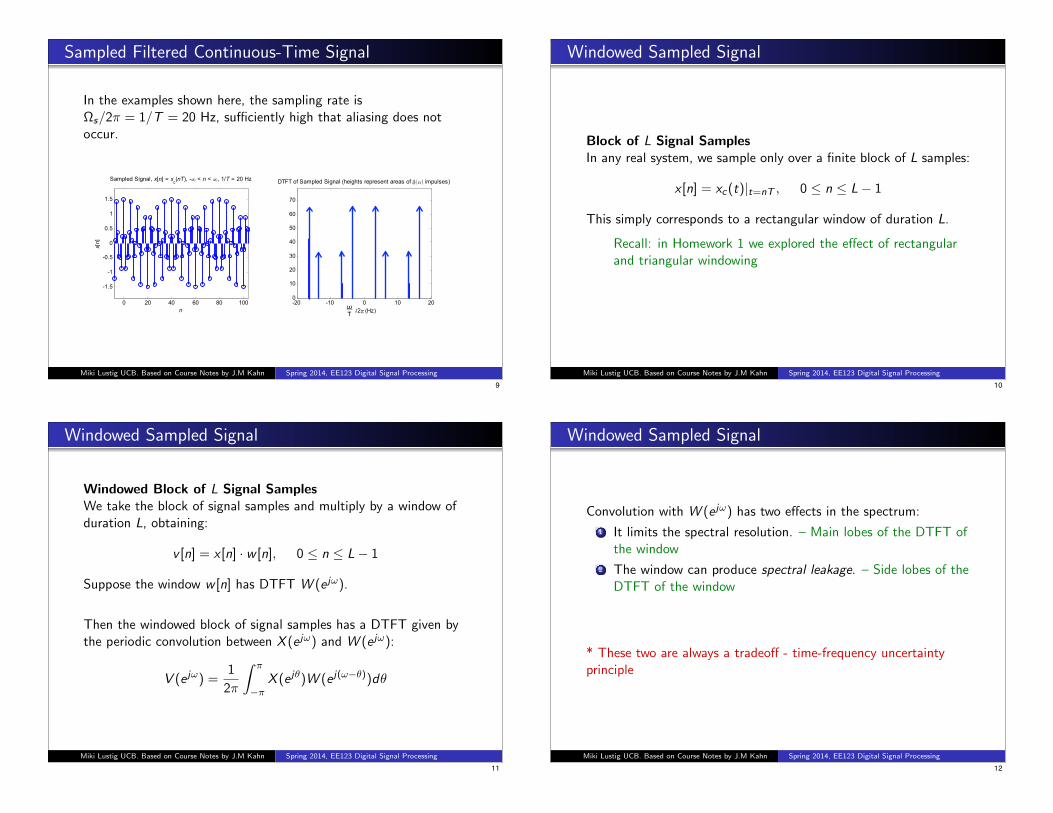
In the examples shown here, the sampling rate is⌦s

/2⇡ = 1/T = 20 Hz, su�ciently high that aliasing does notoccur.

0 20 40 60 80 100

-1.5

-1

-0.5

0

0.5

1

1.5

n

x[n]

Sampled Signal, x[n] = xc(nT), - < n < , 1/T = 20 Hz

-20 -10 0 10 200

10

20

30

40

50

60

70

/2 (Hz)

X(ejT)

DTFT of Sampled Signal (heights represent areas of ( ) impulses)


ωT

Ω

9

Windowed Sampled Signal

Block of L Signal SamplesIn any real system, we sample only over a finite block of L samples:

x [n] = x

c

(t)|t=nT

, 0 n L� 1

This simply corresponds to a rectangular window of duration L.

Recall: in Homework 1 we explored the e↵ect of rectangularand triangular windowing


10


Windowed Block of L Signal SamplesWe take the block of signal samples and multiply by a window ofduration L, obtaining:

v [n] = x [n] · w [n], 0 n L� 1

Suppose the window w [n] has DTFT W (e j!).

Then the windowed block of signal samples has a DTFT given bythe periodic convolution between X (e j!) and W (e j!):

V (e j!) =1

2⇡

Z ⇡

�⇡X (e j✓)W (e j(!�✓))d✓


11


Convolution with W (e j!) has two e↵ects in the spectrum:

1 It limits the spectral resolution. – Main lobes of the DTFT ofthe window

2 The window can produce spectral leakage. – Side lobes of theDTFT of the window

* These two are always a tradeo↵ - time-frequency uncertaintyprinciple


12

Windows (as defined in MATLAB)

-5 0 50

0.2

0.4

0.6

0.8

1

n

w[n

]

boxcar(M+1), M = 8

-5 0 50

0.2

0.4

0.6

0.8

1

n

w[n

]

boxcar(M+1), M = 8

-5 0 50

0.2

0.4

0.6

0.8

1

n

w[n

]

triang(M+1), M = 8

-5 0 50

0.2

0.4

0.6

0.8

1

n

w[n

]

triang(M+1), M = 8

-5 0 50

0.2

0.4

0.6

0.8

1

n

w[n

]

bartlett(M+1), M = 8

-5 0 50

0.2

0.4

0.6

0.8

1

n

w[n

]

bartlett(M+1), M = 8

Name(s) Definition MATLAB Command Graph (M = 8)

Rectangular

Boxcar

Fourier

nw20

21

Mn

Mnboxcar(M+1)

Triangular nw

20

212

1

Mn

MnM

n

triang(M+1)

Bartlett nw

20

22

1

Mn

MnM

n

bartlett(M+1)


13

Windows (as defined in MATLAB)

-5 0 50

0.2

0.4

0.6

0.8

1

n

w[n

]

hann(M+1), M = 8

-5 0 50

0.2

0.4

0.6

0.8

1

n

w[n

]

hann(M+1), M = 8

-5 0 50

0.2

0.4

0.6

0.8

1

n

w[n

]

hanning(M+1), M = 8

-5 0 50

0.2

0.4

0.6

0.8

1

n

w[n

]

hanning(M+1), M = 8

-5 0 50

0.2

0.4

0.6

0.8

1

n

w[n

]

hamming(M+1), M = 8

-5 0 50

0.2

0.4

0.6

0.8

1

n

w[n

]

hamming(M+1), M = 8

Name(s) Definition MATLAB Command Graph (M = 8)

Hann nw

20

22

cos12

1

Mn

MnM

n

hann(M+1)

Hanning nw

20

212

cos12

1

Mn

MnM

n

hanning(M+1)

Hamming nw

20

22

cos46.054.0

Mn

MnM

n

hamming(M+1)


14

Windows

All of the window functions w [n] are real and even.

All of the discrete-time Fourier transforms

W (e j!) =

M

2X

n=�M

2

w [n]e�jn!

are real, even, and periodic in ! with period 2⇡.

In the following plots, we have normalized the windows to unitd.c. gain:

W (e j0) =

M

2X

n=�M

2

w [n] = 1

This makes it easier to compare windows.


15

Window Example

0 0.5 1 1.5 2 2.5 3

-0.2

0

0.2

0.4

0.6

0.8

1

W(ej

)

M = 16

Boxcar

Triangular

0 0.5 1 1.5 2 2.5 3

-0.2

0

0.2

0.4

0.6

0.8

1

W(ej

)

M = 16

Hanning

Hamming

0 0.5 1 1.5 2 2.5 3-70

-60

-50

-40

-30

-20

-10

0

20

lo

g1

0|W

(ej

)|

M = 16

Boxcar

Triangular

0 0.5 1 1.5 2 2.5 3-70

-60

-50

-40

-30

-20

-10

0

20

lo

g1

0|W

(ej

)|

M = 16

Hanning

Hamming


ωω

ω ω

16

–fft ee123 •today frequency analysis with dft …ee123/sp14/notes/lecture08...spectral analysis...

Documents