RICARDO A. MADEIRA

WORKING PAPER SERIES Nº 2012-26

Department of Economics- FEA/USP

The Effects of Decentralization on Schooling: Evidence From the Sao Paulo State’s Education Reform

DEPARTMENT OF ECONOMICS, FEA-USP WORKING PAPER Nº 2012-26

The Effects of Decentralization on Schooling: Evidence from the Sao Paulo State's Education Reform

Ricardo A. Madeira (rmadeira@usp.br)

JEL Codes: I2, I28, H43, H7, C21

Keywords: Decentralization of Public Services, Education Economics, School Quality and Program Evaluation

Abstract:

Decentralization of the delivery of public services provision is an important governance reform recently witnessed in many developing countries. Public education has been one of the key public services devolved to lower level governments. This paper uses an exclusive and rich longitudinal data on primary schools to evaluate the effects of the decentralization reform implemented on the State of Sao Paulo, Brazil, on several indicators of school performance and school resources. Specific aspects of the Sao Paulo’s State education reform combined with the data available allow me to deal with some common identification issues encountered by previous empirical studies on the subject. I find conflicting results for different school quality measures; decentralization increased dropout rates and failure rates across all primary school grades but improved several school resources. Further empirical investigation suggests that the worsening of these school performance indicators for the two first grades was partially driven by the democratization of the school access promoted by the education reform. Evaluation of the distributive outcome of the reform suggests that its effects were more perverse for schools located on rural and poor areas. I also find evidence that decentralization widened the gap between the “good” and “bad” schools. Moreover, I find no evidence that the municipalities’ administrative experience affected the program’s outcome.

The Effects of Decentralization on Schooling: Evidence Fromthe Sao Paulo State’s Education Reform

Ricardo Madeira∗*University of São Paulo

September 2012

Abstract

Decentralization of the delivery of public services provision is an important governance reformrecently witnessed in many developing countries. Public education has been one of the key publicservices devolved to lower level governments. This paper uses an exclusive and rich longitudinaldata on primary schools to evaluate the effects of the decentralization reform implemented onthe State of Sao Paulo, Brazil, on several indicators of school performance and school resources.Specific aspects of the Sao Paulo’s State education reform combined with the data available allowme to deal with some common identification issues encountered by previous empirical studieson the subject. I find conflicting results for different school quality measures; decentralizationincreased dropout rates and failure rates across all primary school grades but improved severalschool resources. Further empirical investigation suggests that the worsening of these schoolperformance indicators for the two first grades was partially driven by the democratization ofthe school access promoted by the education reform. Evaluation of the distributive outcome ofthe reform suggests that its effects were more perverse for schools located on rural and poorareas. I also find evidence that decentralization widened the gap between the “good”and “bad”schools. Moreover, I find no evidence that the municipalities’administrative experience affectedthe program’s outcome.

Keywords: Decentralization of Public Services, Education Economics, School Quality andProgram Evaluation.

JEL Classifications: I2, I28, H43, H7 and C21

∗Department of Economics, Boston University. 270 Bay State Rd., Boston, MA 02215, USA; e-mail:rmadeira@bu.edu. I thank Dilip Mookherjee, Kevin Lang, Victor Aguirregabiria, Patricia Meirelles, Daulins Emilio,Gabriel Madeira, Marcos A. Rangel and participants of the BU empirical micro seminar for their helpful comments. Ihave benefited from discussions about the “Municipalizacao do Ensino”program with several scholars and governmentoffi cials, I am especially thankful to Hubert Alqueres, Neide Cruz, Felicia Madeira and Rose Neubauer. Financial sup-port from the Boston University’s Institute of Economic Development (IED) and the Brazilian Ministry of Science andTechnology (CNPq) were essential for the realization of this paper. I am also extremely thankful to Eliana Rodrigueswho provided excellent assistance with the manipulation of the GIS data. All remaining errors are mine.

1

1 Introduction

The decentralization of public services has been one of the most common governance reforms

implemented by developing countries. Decentralization reforms are commonly justified by the

belief that local governments are more accountable and responsive to the needs of their local

communities. It is believed that the proximity of elected local offi cials to their communities

gives them an informational advantage over higher-level governments concerning the local

communities’preferences, thus enhancing their ability to tailor public services delivery to the

communities’demand. Moreover it is contended that as a result from political competition

in local government, decentralization may promote innovation, experimentation and learning

about service delivery policies.

On the other hand, the existing literature on decentralization also points to some possible

impediments to the success of decentralization reform. One of the major obstacles involves

the greater susceptibility of the local governments to being captured by local elites, in the

sense that service provision may be designed to cater to the interests of local special interest

groups. This threat is believed to be particularly relevant for unequal and poor communities,

where the impoverished tend to be more alienated from the political process. It has also

been argued that local governments do not have the necessary administrative competence to

provide public services effi ciently. In addition, the existence of local public goods externalities

that go beyond the jurisdiction of local governments, combined with a low coordination effort

among them, compromises the effi ciency of service delivery under the decentralized regime.

Finally, the devolution of administrative responsibilities unmatched with the devolution of

fiscal autonomy may result on unfunded mandates. That is, if the necessary fiscal resources

to manage the new administrative responsibilities are not granted to the local governments,

the local services provision will suffer from scarcity of investments.

Under the existence of many favorable and unfavorable theoretical arguments, the consen-

sus in the decentralization literature is that decentralization outcomes are context-dependent

and must be settled by the conduct of empirical research. To that end, this paper employs

exclusive and rich longitudinal data on primary schools to evaluate the effects of the decen-

tralization reform implemented in the State of Sao Paulo, Brazil (known as "Municipalizacao

do Ensino"), on several indicators of school performance and school resources. Specific as-

pects of the Sao Paulo’s State education reform, combined with the available data, allow me

to tackle some common identification issues encountered by previous empirical studies on the

subject. Moreover, the availability of socio-economic data at the school neighborhood level

combined with socio-economic characteristics and political and fiscal data at the municipality

2

level, allow me to investigate whether there is any empirical evidence that some of channels

addressed in the literature through which decentralization affects service delivery, is at play

in the Sao Paulo context.

Owing primarily to the lack of detailed, disaggregated and longitudinal data, and the con-

stant discontinuity in the implementation of decentralization reforms in developing countries,

most empirical studies have not been able to satisfactorily identify the effects of decentral-

ization. Most of the existing evidence is contained in descriptive study cases based on small

sample analyses that lack the rigor and generality of inferences based on deeper econometric

analysis. The few rigorous empirical studies available on the decentralization effect on service

delivery in general have found conflicting results.1Faguet (2004), has found that the broad

1994’s decentralization reform implemented in Bolivia increased the responsiveness of public

policies to the local needs. Some other studies, however, have found evidence of local elite

capture. Bardhan and Mookherjee’s (2006) findings suggest the presence of elite capture in

inter-village allocation of pro-poor programs in West Bengal. Araujo et. al (2006), using

data on Ecuadorian villages, also uncovered evidence of the influence of local elites on the

village’s choice among social programs offered by the central government.

There is a growing empirical literature on the decentralization of education provision, since

public education has been one of the key public services devolved to lower level governments.

The findings also point to distinct directions. King and Ozler (1998) use cross-sectional data

on students’standardized test scores and their characteristics to evaluate the effect of the

devolution of several management decisions to the schools as a result of Nicaragua school

autonomy reform. To identify the decentralization effect, they take advantage of the time

variation wherein schools were under the decentralized regime and the fact some schools were

not decentralized. Using a two-stage procedure to control for school self-selection into the

program, they find that the devolution of the responsibilities that effectively increases school

autonomy has a positive impact on student performance. Jimenez and Sawada (1998) use

the El Salvador decentralization program to evaluate the effect of the delegation of school

administrative responsibilities to local communities on student attendance and test scores.

Employing cross-sectional student level data and a control group formed by students in non-

decentralized schools, they find that the program had no effect on test scores and diminished

student absence caused by teacher absence. They control for the possible selection bias

imposed by the students’school choice using the Heckman’s two-stage procedure. The main

concern with the empirical strategy adopted by both King and Ozler (1998) and Jimenez1Bardhan and Mookherjee (2005a) present a survey with some of the most relevant empirical evidence.

3

and Sawada (1998) is that their identification of the decentralization effect relies on a correct

specification of the selection equation, even though the causes of the possible selection bias in

either context is different. In Nicaragua, the schools self-select themselves into the program,

while in El Salvador, the students could choose the type of school (centralized or autonomous).

Rodriguez (2006) uses a panel on Colombian municipalities to asses the impact of decen-

tralization on the difference between public and private school average grades on standardized

tests. Her findings suggest that once one accounts for the increase in enrollment on public

schools promoted by the reform, the decentralization improved student performance. Gal-

liani et all (2005) use school-level data on standardized tests in Argentina to evaluate the

effect of school decentralization on student performance. They find that decentralization

improved test performance in the most affl uent municipalities located in well administered

provinces, while it decreased performance in the poorest municipalities located in weakly

administered provinces. Their results are consistent with the theoretical prediction that the

success of decentralization is related to low poverty rates and the local government’s ad-

ministrative ability. Since the identification of the decentralization effect in both papers,

Rodriguez (2006) and Galiani et all (2005), stems from the variation on the timing of the

decentralization across provinces, their identification strategy relies on the assumption that

these variations are exogenously determined.

Paes de Barros and Mendonca (1998) use a state-level panel in Brazil to evaluate the im-

pact of three innovations in school autonomy on several school quality measures and on state

average student performance on standardized tests. The innovations are direct elections of

school principals, the establishment of school councils with members from local communities,

and school financial autonomy. They find very weak evidence that these innovations had

positive effects on schooling. Their econometric strategy also relies on the assumption that

the implementation of these innovations is exogenous.

The “Municipalizacao do Ensino” program was launched in 1996 by the newly elected

government of the State of Sao Paulo. The reform was characterized by the transference of the

full management control of the primary and secondary state-run schools to the municipalities.

Different from most decentralization programs examined in the literature in the Sao Paulo

reform the decision to decentralize was also decentralized. That is, the atate government

devolved to each municipality the decision to take over the primary and secondary state

schools located within its jurisdiction. The municipalities were allowed to make this decision

at any time on a school-by-school basis. The data reveal that the municipalities’participation

in the program was gradual. Other two distinctive features of the Sao Paulo educational

4

reform were its long continuity and size. The state government administration maintained

the reform after winning two subsequent state elections (in 1998 and 2002). In the eight-year

period covered by the data (from 1996 to 2003), more than 2,200 primary state schools were

adopted by the municipalities, which is more than 50% of the state-run primary schools.

In the light of the existing literature, the contribution of this paper is threefold. First,

the fact that the Sao Paulo reform school decentralization was gradual and not universal,

combined with the availability of data on the pre-decentralization period, allows for the im-

plementation of two compelling robustness checks on the identification assumptions of the

econometric specifications used. The robustness exercises performed allow me to identify if

the econometric specifications used are controlling for possible selection biases imposed by the

municipalities’school choice. Second, the availability of data on measures of school resources

and school performance at the school and grade level allow me to identify separately the

decentralization effect on various measures of school quality across all school grades. The re-

sults confirm the relevance of this separation for deeper understanding of how decentralization

affected school quality.

The third contribution stems from a distinctive feature of the data used, i.e., it pro-

vides information on socio-economic characteristics of the school neighborhoods, which I

constructed aggregating the population census tract data through the application of GIS

techniques. Information on socio-economic characteristics of the school neighborhood is of

particular relevance for two reasons. First, they can be used as key time varying control

variables to diminish possible selection bias, since several schools neighborhood characteris-

tics are arguably related with the school adoption criteria used by municipalities. Second,

the interaction between decentralization effects with school neighborhood characteristics al-

lows me to identify whether some of these characteristics are relevant for successful of the

reform, as predicted by some of the theoretical studies. That is, it allows for identifying how

socio-economic characteristics of the school immediacy, where are located those who benefit

most from the school, affects program outcome. In the light of the previous findings in the

literature, it is of particular interest to examine the effects of the school immediacy’s poverty

rate and income distribution on the decentralization outcomes.

This paper finds conflicting results for the average reform impact for different dimension

of school outcomes. The decentralization increased dropout rates and failure rates across

all primary school grades, but improved several school resources. The robustness check

performed provides compelling evidence that my findings are free of possible biases imposed

by the mayor’s selection, once the econometric specifications considered allows for school

5

specific-trends. Further empirical investigation using grade level enrollment and performance

measures suggests that the worsening of the school performance indicators for the first and

second grades were partially driven by the democratization of the school access promoted

by the reform. However, the democratization hypothesis does not explain the performance

worsening observed in the third and fourth grades. The results for the distributive outcomes

of the reform indicate that decentralization was slightly more perverse for schools located

in poor and rural neighborhoods. However, different from the findings of other papers on

the literature I do not find a positive decentralization effect for schools located on more

affl uent areas. Interesting results are obtained when the state schools are grouped according

to their dropout rate rank before the program was launched. The findings suggest that

decentralization widened the gap between the “good” schools, the ones with low dropout

rates, and the “bad” schools, the ones with high dropout rates. Finally, I find no evidence

that the administrative experience with primary schooling management played any role on

the effect of decentralization.

This paper is organized into six sections. Section 2 presents the institutional background of

the Sao Paulo educational reform. Section 3 describes the various data sets used and explains

how the final data set was constructed. Section 4 discusses the empirical strategy implemented

along with the key underlining identification assumptions and presents the results of the

robustness checks performed for the choice of the best econometric specifications. Section 5

describes the findings and section 6 presents the concluding remarks.2

2 Institutional Background and Decentralization Reform

The Brazilian pre-college educational system is organized into four levels: preschool (attended

by 6 year-old), primary school (attended by 7 to 10 year-olds), secondary school (attended

by 11 to 14 year-olds) and high school (attended by 15 to 17 year-olds). The primary

school, which is our object of investigation here, comprises four school years, the first four

grades. The basic displines offered at the primary educational level are language (Portuguese),

mathematics, social studies and science.3

The Brazilian constitution dictates that states and municipal governments share the re-

sponsibility for the provision of primary and secondary public education. The proportion of

primary and secondary schools provided by the municipalities and the states varies widely2The tables with the results are displayed on Appendix I and the detailed description of the procedure used to

construct the school neighborhood variables is presented on the Appendix II.3All the basic subjects are taught by the same teacher, and some private schools enhence their curricular activities

additional activities such as physical education and the arts, which are taught by specialized teachers.

6

across the Brazilian states (see Table 1). In 1997, Sao Paulo had the third highest proportion

of students enrolled in state schools among all the 27 Brazilian states.

Sao Paulo State Decentralization Reform: In 1995, the Brazilian Social Democratic

Party (PSDB) won the Sao Paulo’s state government offi ce, after winning the 1994 election.

There was consensus among government offi cials about the ineffi ciency of the highly central-

ized state’s educational system, because two key reasons. First, the existence of numerous

bureaucratic tiers between state government policy makers and the schools’principal, which

imposed impediments to the system’s response to the schools specific needs. Second, the lack

of community involvement in local school management. To tackle these problems, the state

government launched one of the largest decentralization programs ever implemented in the

Brazilian public education system, known as the "Municipalizacao do Ensino.”The reform

was expected to bring the educational policy decision-making closer to the local communities,

since municipal governments are believed to be more accountable to the community demand

than is state government. Moreover the decentralization could increase the involvement of

the communities with the local schools, improving the response of school management to the

communities needs. These arguments were appealing to the Sao Paulo state due to the huge

social and economic differences across the various regions of the state.

Differently from most decentralization programs examined in the literature in the Sao

Paulo reform the decision to decentralize was also decentralized. That is, the state govern-

ment devolved to each municipality the decision to take over the primary and secondary state

schools located within their jurisdiction. The municipalities were allowed to make this deci-

sion at any time on a school-by-school basis. The mayor of each municipality was responsible

for the takeover decision, though the city council had the power to block the mayor’s decision.

The program was characterized not only for its size in terms of the number of pupils affected

(over 5 millions), but also for its long continuity, since the PSDB continued the program after

winning two succeeding state elections in 1998 and 2002.

Once a municipality adopts a school, its students are automatically transferred. State

legislation mandates that public school students must attend the public school nearest their

homes, irrespective of whether it is state or municipal. The transfer of schools was regulated

by state law 40,673, which was further augmented by the state laws 40,889 and 42,778.

Accordingly to the laws, the municipalities have total autonomy over the adopted schools;

they are fully responsible for all school management activities, from setting the school cur-

ricular core to designing the career plans of school professionals. The few restrictions on

7

the school curricular content were some general educational guidelines established by the

Brazilian National Council of Education, which were also applied to the state-run schools.

Upon school adoption, the property rights of all school physical resources, including the

school building itself, are permanently transferred to the municipal government. Some of

the school’s human resources, including school teachers and staff, are temporally lent by the

state to the municipal administration until the municipalities hire their school professionals

to attend the demand of the newly adopted school. The number of school employees lent by

the state varies according to the needs of the municipalities.

Before program implementation, the vast majority of Sao Paulo’s municipalities had ex-

pertise with primary and secondary education provision. They were only responsible for

kindergarten and preschool administration. Therefore, participation in the program repre-

sented a significant administrative challenge for the adopting municipalities as result of the

higher level of administrative complexity involved in primary and secondary education vis-

à-vis the lower levels of education. The municipalities with no past experience with primary

education had one year, accordingly to the law, to hire new professionals and put in place a

school professionals’career plan and a municipal education council (the municipal institution

responsible for setting the municipal school’s curricular content). The law further dictates

that municipalities must meet certain minimum administrative and financial criteria in order

to be able to adopt a school. However, the law does not explicitly specify those criteria. The

task to determine the municipalities’eligibility for the program was delegated to a commis-

sion composed of education experts formed by a staff of the State-Department of Education.

This commission, known as the Decentralization Team, was also responsible for providing

technical and administrative support to the municipalities engaged in the program during

the transition period.

Primary Education Funding: Before describing the decentralization process and its ex-

tents on the Sao Paulo state, it would be helpful to review the laws that regulate educational

funding in Brazil during the decentralization process. In particular, an education funding

reform (known as FUNDEF) implemented in January of 1998 played a major role in shaping

the public resources earmarked to education.

The Brazilian constitution mandates that municipalities and states must spend at least

25% of their tax revenues and transfers on their educational system to accomplish their

constitutional duty. However, until the FUNDEF4 implementation, there was no regulation4FUNDEF stands for Fundo para a Manutencao e Desenvolvimento do Ensino Fundamental e Valorizacao do

Magisterio.

8

in the constitution about how these resources earmarked to education should be spent. Due

to the heterogeneity between states and municipalities with respect to the number of pupils

enrolled in their education system, richer states and municipalities were spending more per

pupil than their poorer counterparts. That is, the allocation of resources earmarked to

education was not driven by the investment necessity. In addition, because the lack of

regulation in the constitutional law about how the earmarked resources should be allocated,

richer states and municipalities could exploit the broad definition of education to spend their

resources earmarked for education in other activities marginally related to education. The

lack of effective monitoring also contributed to this type of moral hazard behavior. This

problem was particularly acute in the municipalities on the Sao Paulo state, since most

of them were only responsible for maintaining a pre-school system, which requires fewer

resources per pupil than higher levels of education.

An additional issue of the pre-FUNDEF education funding law was the lack of specification

of how the earmarked resources should be distributed across various levels of education. For

some researchers (Castro, 1998), this problem was particularly severe, since they contended

that the lack of investments in primary and secondary education was one of the bottlenecks

of the Brazilian public education system.

As an attempt to deal with these distortions, the federal government implemented a

national education bill (FUNDEF), which was approved by the national congress in 1996,

but not implemented until January 1998. The essential features of the FUNDEF are:

i) Create a fund with resources collected from states and municipalities. Each state and

municipality must contribute 15% of its tax revenues and transfer revenues.

ii) Redistribute the resources collected within states to municipalities and state govern-

ment according to the number of students enrolled in their primary and secondary education

system.5

iii) Create a commission to annually set a minimum monetary value per pupil to be

distributed. This minimum value is based on an estimate of school management costs. Due

to the characteristics of various types of schools, this minimum can be different for primary

and secondary schools. If for some states, the resources per pupil collected by the fund are

smaller than the minimum set value, the federal government must provide the difference.6

iv) States and municipalities must spend at least 60% of the fund on teacher wages.

This new educational funding regulation represented a significant change on the fiscal in-

centives for school adoption. During the pre-FUNDEF’s period (1996 and 1997), there was no5The redistribution of resources is based on the School Census data.6 In 1997, the federal government complemented the fund for 6 states

9

pre-established financial compensation in exchange for school adoption. Financial compen-

sations were negotiated in a case-by-case basis, depending on the financial situation of each

municipality and on the number of schools they were willing to adopt. However, FUNDEF

granted to the adopting municipalities the financial resources to manage the schools, since the

fund’s resources were allocated in order to maintain the spending per pupil constant.7 After

its implementation, FUNDEF was the only fiscal incentives for the adopting municipalities,

i.e., the state government dropped all other forms of fiscal compensation.

Decentralization Diffusion Tables 2 and 3 in the appendix describe the diffusion of the

decentralization process. Table 1 compares the yearly evolution of the average municipal

enrollment share on total public enrollment for primary and secondary schools across all the

645 municipalities of the Sao Paulo state. It shows that the program engagement was much

stronger for primary schools. From 1996 to 2003, the average municipal enrollment share

of primary schools climbed from 5.98% to 70.46%, while for secondary school schools the

figures increased from 1.90% to 21.26%. The municipalities could also increase their share

on the total public school enrollment by building their own schools instead of adopting state-

managed schools. However, table 3 shows that decentralization was responsible for more

than half of the observed increase on municipal enrollment in primary schools across the

state. The third column reports the total number of decentralized schools and enrolment

in decentralized schools by year, while the second column presents the same figures for own

municipal schools. By 2003, 2,326 schools had been decentralized, accounting for 60% of the

existing municipal schools across the sate.

The number of state schools adopted by year is presented on the fourth column of Table

3. It reveals that the program participation was gradual on time. The engagement in the

program peaked in 1998 and has decreased at a slow rate since then. This pattern suggests

the important role played by the FUNDEF reform.

The spatial dispersion of the adoption decisions across municipalities over time is depicted

in Figure 1. The municipalities marked in blue are the adopters. The blue scale indicates

the fraction of state schools that were adopted (the darker it is, the higher the fraction of

adopted schools). The figure shows that decentralization diffusion across municipalities was

also gradual. In addition, the figure reveals that many municipalities adopted schools over

time, starting with a few schools and increasing the share of adopted schools in subsequent

years. Lastly, the figure suggests that the adoption decisions by the municipalities are spa-7The FUNDEF was an attempt to discipline 60% of the resources earmarked to education by the constitution.

Castro (1998) shows that the FUNDEF was effectively a fiscal reform within states, given the magnitude of its impactin municipalities and states budget.

10

tially correlated. The sequel of maps, from 1996 to 2003, shows that there were a few pioneers

in 1996; in the following years, cluster of adopters were being built around the 1996 adopters.

3 Data

The final data set used in this paper was assembled by combining four different sources of

Brazilian data: the School Census, Decennial Population Census data, electoral data and

municipalities Fiscal Data.8

School Census: The School Census is an annual survey that collects information on

every school in Brazil, both public and private. The survey is conducted by the Ministry of

Education in collaboration with state-level education departments. Questionnaires are sent

to each school principal and a response is mandatory.9

The data provide detailed information on school resources, such as number of classrooms,

libraries, computer labs, sports facilities, source of water supply, and access to sewerage. The

data also provides the number of teachers per school level and the highest degree of education

obtained by each teacher. At the student level, the School Census provides information on

the number of students per school grade, organized by gender and age. Data on student

performance is also available in the form of failure and dropouts per school grade.

I use data from 1996 to 2003 for all primary (first to fourth grades) schools (public and

private) in the State of Sao Paulo. In 1996, there were 6,615 primary schools in the Sao Paulo

State with 2,327,177 students. In 2003 there were 7,615 primary schools with 2,097,120

students. For the 8-years period covered by this paper, the data provides information on

11,709 primary schools, which comprise the set of all primary schools in the State of Sao

Paulo that were operational at some point during these years.

Decennial Population Census: The Decennial Population Census is the most detailed

Brazilian household survey. It has been collected decennially since 1950 by the Brazilian

Institute of Geography and Statistics (IBGE), an agency of the federal government.10 The8Each of these data sets are publicly available (some upon request) from their administrators. The Decennial

Population Census data can be found at the Sao Paulo state government agency Data Analysis Foundation (SEADE) at<http://www.seade.gov.br/>. The School Census data can be found at the Brazilian Ministry of Education’s websiteat <http://www.mec.gov.br/>. The fiscal data of the Municipality-level Data is available at the website of the SaoPaulo State Account Offi ce (TCE-SP) at <http://www.tce.sp.gov.br/>, and the electoral data is available from theBrazilian Supreme Electoral Court (TSE) at <http://www.tse.gov.br/>.

9 In order to check the accuracy of the information provided a random sample of schools is inspected every year bythe state-level Education Department.10The only exception was in 90’s, where the census was collected in 1991.

11

census data are organized into two different samples, the sample census and the universal

census, both provide household data. The former provides information on the universe of

the Brazilian households, while the later provides more detailed household information for a

sample of 20% of the Brazilian households (every fifth home is surveyed). Most the informa-

tion provided by the universal census is for the head-of-household, while the sample census

contains information on all household members.

This paper uses data from the census tract, which is constructed based on the universal

census, for the years of 1991 and 2003. The census tract is a geographic division of the census

that roughly contains data on 1000 households each; with its borders being defined by the

IBGE according to administrative criteria. I use data on all the 49,713 census tracts that

cover the entire territory of the Sao Paulo State. In 2000, the Sao Paulo State population

was 37,032,403 distributed among 645 municipalities.

For each census tract, there are 527 variables on the characteristics of the households

(mostly head-of-household) who live inside its boundaries. Due to the IBGE confidentiality

policy, census tract micro data are not available; IBGE only provides the marginal distri-

bution of each variable. The variables available are organized into three different groups

according to the type of information. The first group provides information on several home

characteristics, such as type of property (e.g., rented, owned), access to treated water and

sewerage, and number of bathrooms. The second and larger group is composed of variables

on the characteristics of the head-of-household, such as age, gender, income and years of

education. The last group of variables provides information on the other members of the

households, such as number of members, gender, age, and relation to the head-of-household.

This last set of variables does not provide information on the income of the other members

of the household nor detailed information on their education attainment; the only education

information available is on literacy.

Electoral Data: >From 1996 to 2003, four elections were held in Brazil, one every two

years starting from 1996. In the years 1996 and 2000, local elections were held for mayors and

city council and in 1998 and 2002, general elections were held for president, state governor, the

senate, the state congress, and the national congress. The electoral data provide information

on all election outcomes per pooling station, including the number of votes received by all

candidates, political parties, and turnout rate. This paper makes use of data from the four

elections aggregated at the municipal level for all municipalities in the state. I also use data

on the political party of the mayors and on the city councils’political party composition.

12

Fiscal Data: The fiscal data contain yearly information on municipal revenues, expen-

ditures, and deficits. The revenue data are broken down by various sources of taxes and

transfers (e.g., property tax and federal government transfers). The expenditure data are

broken down into 12 areas of public policies, including health, education, housing, trans-

portation, and social security.

Final Data Set: For all the urban municipalities with more than 25,000 habitants in 2000

(which accounts for 170 municipalities out of 645), the IBGE provides digital maps of the

census tract, and the SEADE (Data Analysis Foundation of the State of Sao Paulo) provides

digital street maps. By combining these maps, it becomes possible to identify in which

census tract each school is located through the full school addresses provided by the school

census. Making use of GIS techniques and interpolating the 1991 and the 2000 Decennial

Population Census, I have aggregated the census tract for each public school neighborhood

by year, where the school neighborhood was defined to match the area where are located

the potential public school users accordingly to the Brazilian legislation. The data appendix

explains in more detail how the school neighborhoods were constructed.

The final outcome is an eight-year school level panel, from 1996 to 2003, that includes all

primary schools (private and public) located in the State of Sao Paulo. Besides the school level

information available on the school census data, the panel also contains yearly information

on the census tract household’s variables for the public school neighborhoods and the yearly

information provided by the Electoral and Fiscal data aggregated at the municipal level.

4 Econometric Strategy

In order to obtain a comprehensive understanding of the decentralization effect on the quality

of school provision, we examine its impact on indicators of school performance and school

resource. In doing so, I use three measures of school performance aggregated across the four

primary school grades11: dropout rates, failure rates and age-grade distortion. The dropout

rate is given by the total number of students who have dropped out the school by the end of

the school year divided by total enrollment at the beginning of the school year. The failure

rate is given by the total number of students who failed by the end of the school year divided

by the initial enrollment. The age-grade distortion is given by the average difference between

the students’age and the ideal age of the grade in which they are enrolled. As for school11All the three mesures are first computed at the grade level and than aggregated across the four grades taking

a weighted average, where the weight are given the share of the student enrollment in each grade over total schoolenrollment across grades.

13

resources, we use seven different indicators; class size, pupil-teacher ratio, hours of schooling,

percentage of teachers with college degree, number of computers per hundred pupils, number

of television per hundred pupils and number of VCRs per hundred pupils.

A major econometric concern for estimating the impact of the decentralization on these

school quality indicators stems from the fact that the municipalities selected themselves into

the program, i.e., the decentralization was not randomly assigned. Therefore, observed differ-

ences in quality between the decentralized and non-decentralized schools could potentially be

driven by the adoption criteria used by the mayors, rather than the decentralization reform.

The hypothetical counterfactual exercise that one would like to perform to accurately access

the decentralization effect on the school quality indicators involves comparing at the same

time the quality indicators of the same school under the two type of administration, state

and municipal. Since this is not feasible, my identification strategy relies on the difference-in-

differences approach proposed by the treatment effect literature for non-random treatments.

The rationale for this approach is to compare the school quality indicators of the decentralized

schools (treated) to the same indicators of a control group of schools, which are not affect by

the decentralization. A valid control group must include non-decentralized schools where the

average school quality indicators would not differ from the decentralized ones on the absence

of decentralization. In other words, the control group should provide a good proxy for the

decentralized schools in the absence of the decentralization.

Based on that, my identification strategy relies on three factors: (i) the fact the school

adoption was gradual in time, (ii) the availability of panel data with information before and

after the decentralization, and (iii) the availability of several time varying control variables

that are possibly correlated with the adoption decision and the decentralization effect on

school quality. The combination of the first and second factors allows me to use as a control

group all state managed schools that were never decentralized and all the decentralized state

schools before the decentralization.12 In addition, the availability of panel data allows me

to control for all time invariant school’s unobserved heterogeneities that might be correlated

to the adoption decision and the decentralization effect. Lastly, the availability of several

time varying variables at the school, school neighborhood and municipality level allows me

to control for key time varying elements that might be related with the mayors’ choice.

Therefore, unless the mayors based their school adoption decisions on some unobservable

time varying characteristic that affects the decentralization outcome on the school quality

measures, one of the econometric specifications considered should provide unbiased estimates12For all schools decentralized after 1996, which comprises 96% of them, there are data available on the quality

indicators before an after the decentralization.

14

of decentralization effect. Given the large set of time varying controls available, it is diffi cult

to thing of any possible unobservable time varying school and municipality characteristics

that could possibly affect the impact of the reform on school quality.

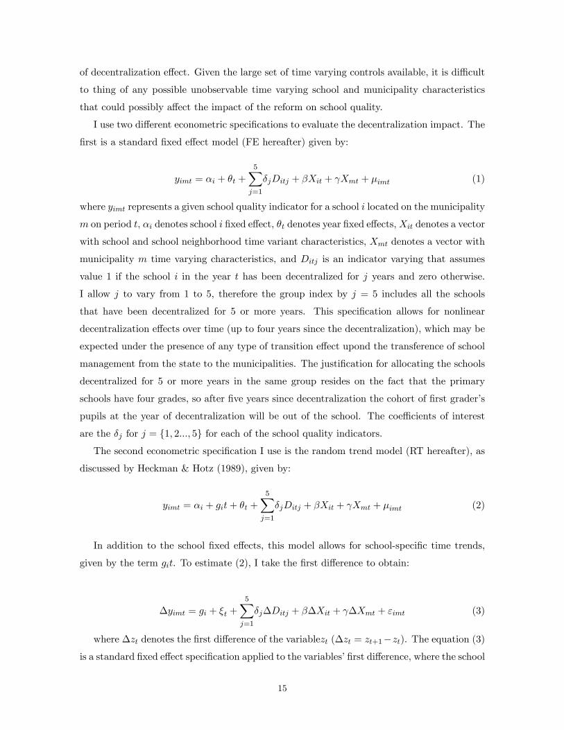
I use two different econometric specifications to evaluate the decentralization impact. The

first is a standard fixed effect model (FE hereafter) given by:

yimt = αi + θt +

5∑j=1

δjDitj + βXit + γXmt + µimt (1)

where yimt represents a given school quality indicator for a school i located on the municipality

m on period t, αi denotes school i fixed effect, θt denotes year fixed effects,Xit denotes a vector

with school and school neighborhood time variant characteristics, Xmt denotes a vector with

municipality m time varying characteristics, and Ditj is an indicator varying that assumes

value 1 if the school i in the year t has been decentralized for j years and zero otherwise.

I allow j to vary from 1 to 5, therefore the group index by j = 5 includes all the schools

that have been decentralized for 5 or more years. This specification allows for nonlinear

decentralization effects over time (up to four years since the decentralization), which may be

expected under the presence of any type of transition effect upond the transference of school

management from the state to the municipalities. The justification for allocating the schools

decentralized for 5 or more years in the same group resides on the fact that the primary

schools have four grades, so after five years since decentralization the cohort of first grader’s

pupils at the year of decentralization will be out of the school. The coeffi cients of interest

are the δj for j = {1, 2..., 5} for each of the school quality indicators.The second econometric specification I use is the random trend model (RT hereafter), as

discussed by Heckman & Hotz (1989), given by:

yimt = αi + git+ θt +5∑j=1

δjDitj + βXit + γXmt + µimt (2)

In addition to the school fixed effects, this model allows for school-specific time trends,

given by the term git. To estimate (2), I take the first difference to obtain:

∆yimt = gi + ξt +5∑j=1

δj∆Ditj + β∆Xit + γ∆Xmt + εimt (3)

where ∆zt denotes the first difference of the variablezt (∆zt = zt+1−zt). The equation (3)is a standard fixed effect specification applied to the variables’first difference, where the school

15

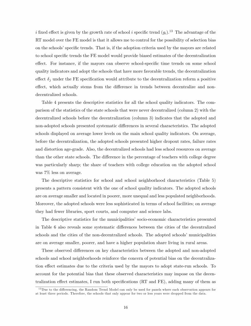
i fixed effect is given by the growth rate of school i specific trend (gi).13 The advantage of the

RT model over the FE model is that it allows me to control for the possibility of selection bias

on the schools’specific trends. That is, if the adoption criteria used by the mayors are related

to school specific trends the FE model would provide biased estimates of the decentralization

effect. For instance, if the mayors can observe school-specific time trends on some school

quality indicators and adopt the schools that have more favorable trends, the decentralization

effect δj under the FE specification would attribute to the decentralization reform a positive

effect, which actually stems from the difference in trends between decentralize and non-

decentralized schools.

Table 4 presents the descriptive statistics for all the school quality indicators. The com-

parison of the statistics of the state schools that were never decentralized (column 2) with the

decentralized schools before the decentralization (column 3) indicates that the adopted and

non-adopted schools presented systematic differences in several characteristics. The adopted

schools displayed on average lower levels on the main school quality indicators. On average,

before the decentralization, the adopted schools presented higher dropout rates, failure rates

and distortion age-grade. Also, the decentralized schools had less school resources on average

than the other state schools. The difference in the percentage of teachers with college degree

was particularly sharp; the share of teachers with college education on the adopted school

was 7% less on average.

The descriptive statistics for school and school neighborhood characteristics (Table 5)

presents a pattern consistent with the one of school quality indicators. The adopted schools

are on average smaller and located in poorer, more unequal and less populated neighborhoods.

Moreover, the adopted schools were less sophisticated in terms of school facilities; on average

they had fewer libraries, sport courts, and computer and science labs.

The descriptive statistics for the municipalities’socio-economic characteristics presented

in Table 6 also reveals some systematic differences between the cities of the decentralized

schools and the cities of the non-decentralized schools. The adopted schools’municipalities

are on average smaller, poorer, and have a higher population share living in rural areas.

These observed differences on key characteristics between the adopted and non-adopted

schools and school neighborhoods reinforce the concern of potential bias on the decentraliza-

tion effect estimates due to the criteria used by the mayors to adopt state-run schools. To

account for the potential bias that these observed characteristics may impose on the decen-

tralization effect estimates, I run both specifications (RT and FE), adding many of them as13Due to the differencing, the Random Trend Model can only be used for panels where each observation appears for

at least three periods. Therefore, the schools that only appear for two or less years were dropped from the data.

16

controls. More specifically, I include controls for school characteristics (enrollment, number

of employees, number of classrooms, school levels offered, library, science lab, computer lab

and sports court), school neighborhood and cities’socio-economic characteristics (population,

percentage of population on the primary schooling age range, average income, and income’s

coeffi cient of variation). For the school performance regressions all the measures of school

resources were also added to the controls.

Although the descriptive statistics for the municipalities (Table 6) do not suggest any

sharp differences between the political characteristics of the adopting and non-adopting mu-

nicipalities, key political characteriscs relevant for the decentralization process were included

nonetheless among the set of controls. Since the reform was proposed by the Brazilian Social

Democrat Party (PSDB), it is reasonable to conjecture that the mayor’s party affi liation

played a role on their decision to engage in the program. That is, it is possible that the

mayors whose political party is closer to PSDB were more prone to engage in the program.

To account for possible biases imposed by school adoptions induced by the mayor’s party

affi liation, a dummy variable that indicates if the PSDB belongs to the mayor’s coalition on

the municipal election was included among the controls. Also, since the city council has the

power to block the mayor’s adoption decision, I also added among the set of controls the

share of the city council members who belong to the coalition of the mayor’s party. Finally,

I also include among the city level controls revenue per-capita and a dummy variable that

indicates if the city is running a fiscal deficit or surplus (budget status).

4.1 Specification Choice

Table 7 displays the results for the FE model, while table 9 presents the results for the RT

model. The “sample year”row on tables indicates the years that were included in the sample

for each regression. Since some of the controls are only available for more recent years, due to

changes on the School Census questionnaire through the years, I present the regressions for

different years to allow for the inclusion of additional controls.1415 The dependent variable

student age-grade distortion and percentage teachers with college education are only available

after 1997.

Apart from the magnitude of effects, both specifications present similar results for school14A potential relevant control that was only included on the School Census survey after 1997 is the existence automatic

promotion policy. Schools that have adopted this policy only fail students who have extremely bad performances relatedto clear lack of effort and high school absence. Therefore is natural to expect that this policy affect students’performance.15 I also run all the regressions without the inclusion of school characteristics and school resources among the controls,

since the decentralization could be affecting the school quality indicators through changes in these resources. The resultsobtained with the omission of these variables are quite similar and are available under request. These results will showon a future version of this paper.

17

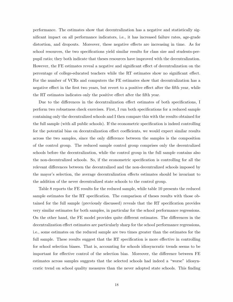
performance. The estimates show that decentralization has a negative and statistically sig-

nificant impact on all performance indicators, i.e., it has increased failure rates, age-grade

distortion, and dropouts. Moreover, these negative effects are increasing in time. As for

school resources, the two specifications yield similar results for class size and students-per-

pupil ratio; they both indicate that theses resources have improved with the decentralization.

However, the FE estimates reveal a negative and significant effect of decentralization on the

percentage of college-educated teachers while the RT estimates show no significant effect.

For the number of VCRs and computers the FE estimates show that decentralization has a

negative effect in the first two years, but revert to a positive effect after the fifth year, while

the RT estimates indicates only the positive effect after the fifth year.

Due to the differences in the decentralization effect estimates of both specifications, I

perform two robustness check exercises. First, I run both specifications for a reduced sample

containing only the decentralized schools and I then compare this with the results obtained for

the full sample (with all public schools). If the econometric specification is indeed controlling

for the potential bias on decentralization effect coeffi cients, we would expect similar results

across the two samples, since the only difference between the samples is the composition

of the control group. The reduced sample control group comprises only the decentralized

schools before the decentralization, while the control group in the full sample contains also

the non-decentralized schools. So, if the econometric specification is controlling for all the

relevant differences between the decentralized and the non-decentralized schools imposed by

the mayor’s selection, the average decentralization effects estimates should be invariant to

the addition of the never decentralized state schools to the control group.

Table 8 reports the FE results for the reduced sample, while table 10 presents the reduced

sample estimates for the RT specification. The comparison of theses results with those ob-

tained for the full sample (previously discussed) reveals that the RT specification provides

very similar estimates for both samples, in particular for the school performance regressions.

On the other hand, the FE model provides quite different estimates. The differences in the

decentralization effect estimates are particularly sharp for the school performance regressions,

i.e., some estimates on the reduced sample are two times greater than the estimates for the

full sample. These results suggest that the RT specification is more effective in controlling

for school selection biases. That is, accounting for schools idiosyncratic trends seems to be

important for effective control of the selection bias. Moreover, the difference between FE

estimates across samples suggests that the selected schools had indeed a “worse” idiosyn-

cratic trend on school quality measures than the never adopted state schools. This finding

18

is consistent with the descriptive statistics presented before, since on average the adopted

schools were located in rural, poorer and more unequal neighborhoods.

For the second robustness check exercise, I take advantage of data availability for the pre

decentralization period to perform the pre-program specification test for non-experimental

estimators.16 This test is executed in two steps. First, I selected all the schools that were

decentralized between 2000 and 2003 and I then run all regressions for both specifications for

a further reduced sample containing only the 2000-2003 period. In the second step, I lagged

the “years since decentralization”17 variable in four years for all the after-2000 decentralized

schools and I then run both specifications (all regressions) for the 1996-1999 sample and

compare them with the results obtained for the 2000-2003 sample. If the specifications are

indeed capturing the average decentralization effect, the estimates for the 1996-1999 sample

should not be significant, since these school were only decentralized after 1999. The results for

this test for the school performance regressions are reported in Table 11, and the results for

the school resource regressions are reported in Table 12. Both specifications for all regressions

pass the test, that is, they provide non-significant effects (at the 5% level or lower) for the

1996-1999 sample even when significant effects are obtained on the 2000-2003 sample.

5 Results

5.1 Average Effects

The two robustness checks performed here suggest that the RT model provides unbiased es-

timates of the average decentralization effect.18 According to the findings of the RT model,

decentralization has on average decreased school performance and improved most school re-

sources. The results for school performance reveal that the negative effects are increasing

over time, suggesting that they are not transitory effects related to possible temporary ad-

justments to the new decentralized regime. The comparison of decentralization effects to the

dependent variables’standard deviations shows that the effect is quite relevant for dropout16An example of the application of this test can be found in Heckman and Hotz (1989).17Since the 1996-1999 and 2000-2003 samples are comprised of four years, to perform the pre-program specification the

decentralization variables5∑j=1

δjDitj in the specifications (1) and (2) were replaced by δDYit, where DYit indicates years

elapsed since the decentralization occurred. Therefore this specification does not allow for nonlinear decentralizationeffects.18Under the presence of serial correlation in the error term, the standard errors of the decentralization effect estimates

could be understated. In a future version of this paper I intend to correct the standard errors using the block-bootstrappingsuggested by Bertrand, Duflo and Mullainathan (2004). However, it should be noted that since the data has a shorttime series, only 8 periods, the existence of serial correlation in the error term is not expected to have a major impactin understating the standard errors. In addition, the fact that the standard errors are clustered at municipal levelmitigates the effects of serial correlation on the standard error.

19

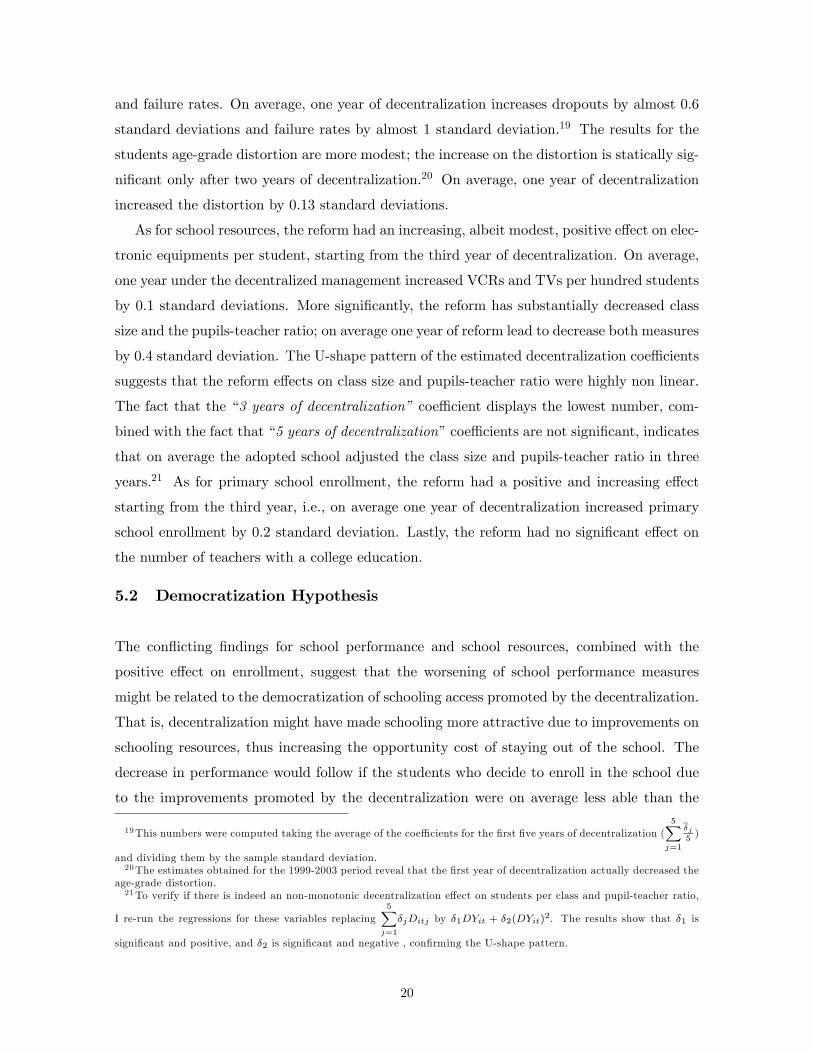
and failure rates. On average, one year of decentralization increases dropouts by almost 0.6

standard deviations and failure rates by almost 1 standard deviation.19 The results for the

students age-grade distortion are more modest; the increase on the distortion is statically sig-

nificant only after two years of decentralization.20 On average, one year of decentralization

increased the distortion by 0.13 standard deviations.

As for school resources, the reform had an increasing, albeit modest, positive effect on elec-

tronic equipments per student, starting from the third year of decentralization. On average,

one year under the decentralized management increased VCRs and TVs per hundred students

by 0.1 standard deviations. More significantly, the reform has substantially decreased class

size and the pupils-teacher ratio; on average one year of reform lead to decrease both measures

by 0.4 standard deviation. The U-shape pattern of the estimated decentralization coeffi cients

suggests that the reform effects on class size and pupils-teacher ratio were highly non linear.

The fact that the “3 years of decentralization” coeffi cient displays the lowest number, com-

bined with the fact that “5 years of decentralization”coeffi cients are not significant, indicates

that on average the adopted school adjusted the class size and pupils-teacher ratio in three

years.21 As for primary school enrollment, the reform had a positive and increasing effect

starting from the third year, i.e., on average one year of decentralization increased primary

school enrollment by 0.2 standard deviation. Lastly, the reform had no significant effect on

the number of teachers with a college education.

5.2 Democratization Hypothesis

The conflicting findings for school performance and school resources, combined with the

positive effect on enrollment, suggest that the worsening of school performance measures

might be related to the democratization of schooling access promoted by the decentralization.

That is, decentralization might have made schooling more attractive due to improvements on

schooling resources, thus increasing the opportunity cost of staying out of the school. The

decrease in performance would follow if the students who decide to enroll in the school due

to the improvements promoted by the decentralization were on average less able than the

19This numbers were computed taking the average of the coeffi cients for the first five years of decentralization (5∑j=1

δ̂j5)

and dividing them by the sample standard deviation.20The estimates obtained for the 1999-2003 period reveal that the first year of decentralization actually decreased the

age-grade distortion.21To verify if there is indeed an non-monotonic decentralization effect on students per class and pupil-teacher ratio,

I re-run the regressions for these variables replacing5∑j=1

δjDitj by δ1DYit + δ2(DYit)2. The results show that δ1 is

significant and positive, and δ2 is significant and negative , confirming the U-shape pattern.

20

students who would enroll in the school in the absence of the improvements. In this case,

decentralization would decrease average student ability, which in turn would result in lower

average student performance. Rodriguez (2006) has identified this democratization effect in

Colombia.

To identify whether the democratization hypothesis can indeed explain the findings for

school performance, I look to the decentralization effect at the grade level. The grade level

regression for dropouts and failure rates show that decentralization has worsened these mea-

sures for all four grades (Tables 13 and 14). The grade enrollment regressions reveal that

decentralization has increased enrollment in the first and second grades, but decrease it on

the third and fourth grades (Table 16). It is thus possible that the democratization hypothe-

sis is valid for the two first grades, but the effects on enrollment argue against the hypothesis

for the last two grades. The second grade enrollment regression provides further evidence of

the democratization hypothesis for the earlier grades since it shows that one year of decen-

tralization has significantly increased enrollment in the second grade. This finding provides

additional evidence that students who were out of the school were contributing to the increase

in second grade enrollment.

It is reasonable to conjecture that the pupils who decide to obtain primary education

as a result of the decentralization-induced increase in the opportunity cost of staying out

of school are on average older than the students who would attend school in the absence

of the decentralization. Accordingly, the positive effect of the decentralization on age-grade

distortion for the second grade (Table 15) provides further support that past primary school

dropouts were contributing to the increase in enrollment, since an increase in the age-grade

distortion means that older students are getting enrolled. In addition, the positive impact

of the decentralization variable on the age-grade distortion for the first grade indicates that

older students were also enrolling in the first grade. Moreover, the fact that the results

show no indication that decentralization has increased the students’age-grade distortion for

the third and fourth grades, where it has decreased enrollment, suggests that older students

indeed contributed to an increase in the overall primary school enrollment.

It is possible that the increase in the student age-distortion promoted by the decentral-

ization was a result of student retention in the school rather than being a consequence of

the enrollment of older students who were out of school. To verify whether student enroll-

ment was indeed driving the results obtained for age-grade distortion, I run the grade level

regression for age-grade distortion while controlling for grade enrollment. If the increase in

enrollment is completely responsible for the increase in the age-grade distortion, we should

21

expect positive and significant coeffi cients for the enrollment variable and a decrease in the

decentralization effect coeffi cients (the higher this decrease, the more enrollment explains the

age-grade distortion). The results are reported in Table 15. The coeffi cients for enrollment

are indeed positive and significant for all grades, except the first grade. Although the in-

clusion of grade enrollment reduces the decentralization coeffi cients, the reduction is quite

modest suggesting that the increase in the age distortion for the first two grades was only

partially driven by the increase in enrollment.

To determine if older pupils are partially responsible for the observed decrease in student

performance, I run a grade level dropout and failure rate regression, adding the grade level

age-grade distortion to the controls. The results for dropout rates reported in Table 13 are

consistent with the democratization hypothesis. They show that the age-grade distortion

variable is positively related to dropouts. Moreover, the inclusion of the age-grade distortion

in the controls reduces the decentralization effect, though the reduction is quite modest.

The results for failure rates (Table 14) corroborate the democratization hypothesis only for

the first grade, since the inclusion of the age-grade distortion reduces the decentralization

effect on the first grade failure rates. But again, the reduction is quite weak. Therefore,

the worsening in performance in the two first grades can be only partially attributed to the

democratization of schooling access promoted by the reform.

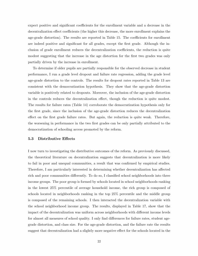
5.3 Distributive Effects

I now turn to investigating the distributive outcomes of the reform. As previously discussed,

the theoretical literature on decentralization suggests that decentralization is more likely

to fail in poor and unequal communities, a result that was confirmed by empirical studies.

Therefore, I am particularly interested in determining whether decentralization has affected

rich and poor communities differently. To do so, I classified school neighborhoods into three

income groups. The poor group is formed by schools located in school neighborhoods ranking

in the lowest 25% percentile of average household income, the rich group is composed of

schools located in neighborhoods ranking in the top 25% percentile and the middle group

is composed of the remaining schools. I then interacted the decentralization variable with

the school neighborhood income group. The results, displayed in Table 17, show that the

impact of the decentralization was uniform across neighborhoods with different income levels

for almost all measures of school quality. I only find differences for failure rates, student age-

grade distortion, and class size. For the age-grade distortion, and the failure rate the results

suggest that decentralization had a slightly more negative effect for the schools located in the

22

poorest areas. As to class size, the results indicate that decentralization has only significantly

improved the school located in more affl uent areas. It thus seems that the decentralization

was more perverse in the poorest communities, but different from the findings of Galiani et all

(2006) in Argentina, there is no evidence that the Sao Paulo reform improved performance on

the richer communities. I further investigate the decentralization distributive effects searching

for differences across rural and urban schools. Table 18 depicts the regression results for the

decentralization effect interacted with an indicator of the region (urban or rural) where the

school is located. The effects on school performance are quite similar across rural and urban

areas. However, the improvements in school resources are only statistically significant for

schools located on urban regions. These results are consistent with those obtained for the

income interaction, since rural areas are poorer than the urban areas on average.

Finally, to identify whether there were any discrepancies on the decentralization effect

between the “good”and “bad”adopted schools, I ranked all the state-run schools that were

not adopted in 1996 according to their dropout rates in 1996, and classified them in three

groups; the 25% highest 1996 dropout (high 1996 dropout), the 25% lowest 1996 (low 1996

dropout) and all the remaining (mid 1996 dropout). Table 19 displays the results for regres-

sions that include the interaction between the decentralization effect and the 1996 dropout

rank classification.22 The estimates reveal a dissimilar effect on good and bad schools (eval-

uated according to 1996 dropout rates). Decentralization has increased the dropout rate

and student age-distortion of the schools that ranked lower in 1996, while it has reduced

these measurers, thought not significantly, for higher ranked schools. As for school resources,

the most striking result stems from the fact that decentralization has decreased the teachers

with a college education in lower ranked schools, while it did not affect the teachers’aver-

age education in the higher ranked schools. The combination of these results suggests that

decentralization has enlarged the gap between the good and bad schools.

5.4 Administrative Experience Effect

The theoretical literature on decentralization argues that in the absence of the necessary

administrative competence in local government, the quality of public service provision may

decrease under the decentralized regime. One may argue that this argument may represent a

real threat to Sao Paulo reform, since before its implementation only few municipalities had

previous experience with primary education management. To test for this effect, I run the

regressions interacting the decentralization effect with a dummy variable that indicates if the22To run these regression I dropped from the data all the schools that were not operational in 1996.

23

municipality managed primary schools before the implementation of the program, in 1996.

The results displayed on Table 20 indicate that the administrative experience with education

did not play any significant role in determining the effect of the reform, since the findings for

the schools located in the experienced and non-experienced municipalities are very similar.

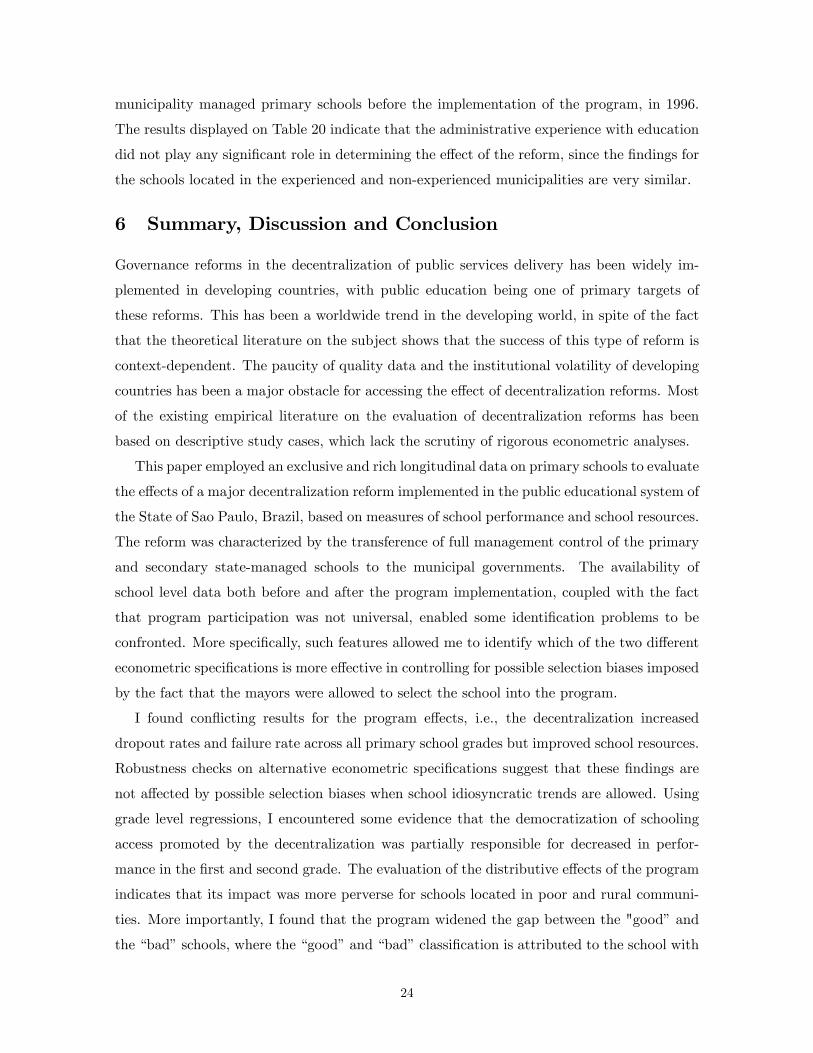
6 Summary, Discussion and Conclusion

Governance reforms in the decentralization of public services delivery has been widely im-

plemented in developing countries, with public education being one of primary targets of

these reforms. This has been a worldwide trend in the developing world, in spite of the fact

that the theoretical literature on the subject shows that the success of this type of reform is

context-dependent. The paucity of quality data and the institutional volatility of developing

countries has been a major obstacle for accessing the effect of decentralization reforms. Most

of the existing empirical literature on the evaluation of decentralization reforms has been

based on descriptive study cases, which lack the scrutiny of rigorous econometric analyses.

This paper employed an exclusive and rich longitudinal data on primary schools to evaluate

the effects of a major decentralization reform implemented in the public educational system of

the State of Sao Paulo, Brazil, based on measures of school performance and school resources.

The reform was characterized by the transference of full management control of the primary

and secondary state-managed schools to the municipal governments. The availability of

school level data both before and after the program implementation, coupled with the fact

that program participation was not universal, enabled some identification problems to be

confronted. More specifically, such features allowed me to identify which of the two different

econometric specifications is more effective in controlling for possible selection biases imposed

by the fact that the mayors were allowed to select the school into the program.

I found conflicting results for the program effects, i.e., the decentralization increased

dropout rates and failure rate across all primary school grades but improved school resources.

Robustness checks on alternative econometric specifications suggest that these findings are

not affected by possible selection biases when school idiosyncratic trends are allowed. Using

grade level regressions, I encountered some evidence that the democratization of schooling

access promoted by the decentralization was partially responsible for decreased in perfor-

mance in the first and second grade. The evaluation of the distributive effects of the program

indicates that its impact was more perverse for schools located in poor and rural communi-

ties. More importantly, I found that the program widened the gap between the "good”and

the “bad”schools, where the “good”and “bad”classification is attributed to the school with

24

high and low dropout rates before program implementation, respectively. Lastly, I did not

uncover any evidence that municipalities’ administrative experience with public schooling

management before the program implementation played any role on its effects.

These findings suggest that local government invested in school resources that make school-

ing more attractive, but is ineffective in keeping pupils in the school. The evidence that

decentralization increased enrollment and the average pupils age in the earlier grades, and

at the same time, increased dropout rates, indicates that the decentralized schools were not

prepared to receive pupils with higher educational deficits. It is possible that the implemen-

tation of the necessary pedagogical changes to deal with this new pool of students requires

school-specific experience and time, which cannot be captured here by the eight year span

of the data. If such is the case, the widening of the gap between the “good’ and “bad”

schools can be explained by the difference of experience in dealing with less able students.

This possibility can also be reconciled with the fact the decentralization was more perverse

in poor and rural areas, since these regions have higher educational deficit.

Another hypothesis that seems to be consistent with this paper’s findings is that decen-

tralization might have adversely affected the pool of students in the school. That is, the more

able students might have left the public school in response to the increase in enrollment of the

less able students promoted by the reform. This would be consistent with the worsening of

school performance and the decrease in enrollment that occurred in third and fourth grades.

Assuming that this effect is increasing in the share of less able students, this hypothesis is

also coherent with the findings for the distributive effects. In a future research, I intend

to investigate this hypothesis by examining the effect of the decentralization on the average

enrollment of private schools located in public school neighborhoods. If this effect turns out

to be present, there should be an increase in private schools’enrollment.

25

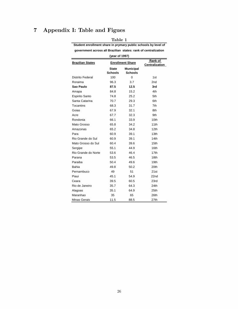
7 Appendix I: Table and Figues

Table 1

Brazilian States  Rank ofCentralization

 StateSchools

MunicipalSchools

Distrito Federal 100 0 1stRoraima 96.3 3.7 2ndSao Paulo 87.5 12.5 3rdAmapa 84.8 15.2 4thEspirito Santo 74.8 25.2 5thSanta Catarina 70.7 29.3 6thTocantins 68.3 31.7 7thGoias 67.9 32.1 8thAcre 67.7 32.3 9thRondonia 66.1 33.9 10thMato Grosso 65.8 34.2 11thAmazonas 65.2 34.8 12thPara 60.9 39.1 13thRio Grande do Sul 60.9 39.1 14thMato Grosso do Sul 60.4 39.6 15thSergipe 55.1 44.9 16thRio Grande do Norte 53.6 46.4 17thParana 53.5 46.5 18thParaiba 50.4 49.6 19thBahia 49.8 50.2 20thPernambuco 49 51 21stPiaui 45.1 54.9 22ndCeara 39.5 60.5 23rdRio de Janeiro 35.7 64.3 24thAlagoas 35.1 64.9 25thMaranhao 35 65 26thMinas Gerais 11.5 88.5 27th

Enrollment Share

Student enrollment share in prymary public schools by level of

government across all Brazilian  states: rank of centralization

(year of 1997)

26

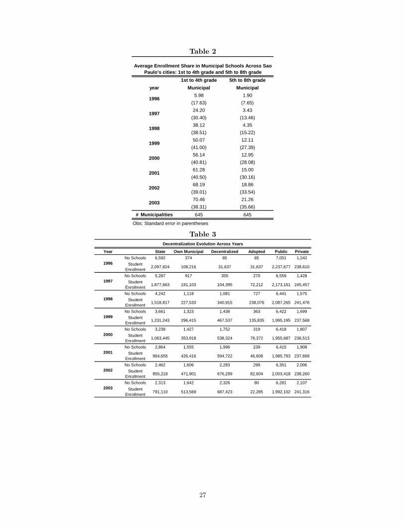
Table 2

1st to 4th grade 5th to 8th gradeyear Municipal Municipal

5.98 1.90(17.63) (7.65)24.20 3.43

(30.40) (13.46)38.12 4.35

(38.51) (15.22)50.07 12.11

(41.00) (27.39)56.14 12.95

(40.81) (28.08)61.28 15.00

(40.50) (30.16)68.19 18.86

(39.01) (33.54)70.46 21.26

(38.31) (35.66)#  Municipalities 645 645

Obs: Standard error in parentheses

Average Enrollment Share in Municipal Schools Across SaoPaulo's cities: 1st to 4th grade and 5th to 8th grade

1996

1997

1998

1999

2000

2001

2002

2003

Table 3

Year State Own Municipal Decentralized Adopted Public PrivateNo Schools 6,592 374 85 85 7,051 1,242

StudentEnrollment 2,097,824 108,216 31,637 31,637 2,237,677 238,610

No Schools 5,287 917 355 270 6,559 1,428Student

Enrollment 1,877,663 191,103 104,395 72,212 2,173,161 245,457

No Schools 4,242 1,118 1,081 727 6,441 1,575Student

Enrollment 1,518,817 227,533 340,915 238,076 2,087,265 241,476

No Schools 3,661 1,323 1,438 363 6,422 1,699Student

Enrollment 1,231,243 296,415 467,537 135,835 1,995,195 237,568

No Schools 3,239 1,427 1,752 319 6,418 1,807Student

Enrollment 1,063,445 353,918 538,324 78,372 1,955,687 236,513

No Schools 2,864 1,555 1,996 239 6,415 1,908Student

Enrollment 964,655 426,416 594,722 46,608 1,985,793 237,669

No Schools 2,462 1,606 2,283 299 6,351 2,006Student

Enrollment 855,218 471,901 676,299 82,604 2,003,418 238,260

No Schools 2,313 1,642 2,326 80 6,281 2,107Student

Enrollment 791,110 513,569 687,423 22,285 1,992,102 241,3162003

1996

1997

1998

1999

2000

2001

2002

Decentralization Evolution Across Years

27

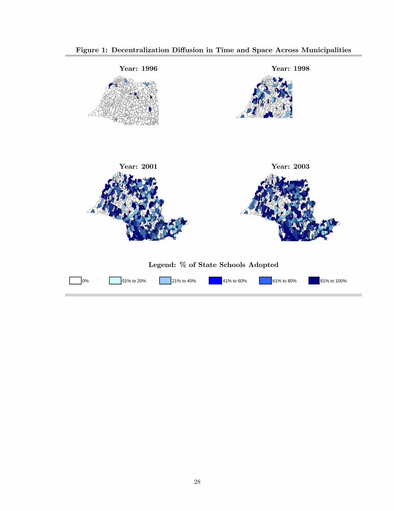
Figure 1: Decentralization Diffusion in Time and Space Across Municipalities

Year: 1996 Year: 1998

Year: 2001 Year: 2003

Legend: % of State Schools Adopted

0% 01% to 20% 21% to 40% 41% to 60% 61% to 80% 81% to 100%

28

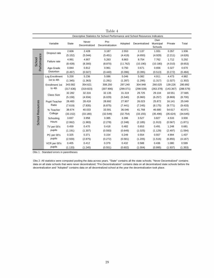
Table 4

Variable State NeverDecentralized

Pre­Decentralization

Adopted DecentralizedOwn

MunicipalSchools

Private Total

2.606 2.428 3.187 2.553 2.137 1.931 0.357 1.936(5.152) (5.044) (5.451) (4.419) (4.650) (4.929) (2.211) (4.626)4.991 4.907 5.263 8.863 8.754 7.762 1.712 5.292

(8.439) (8.300) (8.870) (11.762) (10.190) (10.180) (4.010) (8.653)0.844 0.812 0.961 0.750 0.671 0.656 0.327 0.670

(0.497) (0.507) (0.440) (0.396) (0.395) (0.513) (0.272) (0.484)

5.200 5.236 5.086 5.046 5.082 4.911 4.473 4.982(1.345) (1.363) (1.281) (1.287) (1.295) (1.317) (1.027) (1.302)343.582 354.621 308.250 297.240 304.948 260.025 139.226 280.892

(317.636) (319.823) (307.906) (299.071) (298.539) (263.378) (143.367) (288.579)32.282 32.316 32.135 31.319 29.725 29.104 18.551 27.665(5.158) (4.934) (6.029) (5.540) (5.960) (6.257) (8.869) (8.700)28.483 28.418 28.692 27.907 26.023 25.872 16.141 25.049(7.619) (7.835) (6.875) (7.441) (7.245) (8.175) (9.771) (9.433)38.674 40.033 33.591 36.046 41.768 46.680 54.617 43.971

(33.152) (33.180) (32.549) (32.754) (33.155) (35.496) (35.624) (34.645)3.837 3.958 3.385 3.396 3.527 3.827 4.533 3.930

(2.062) (1.983) (2.278) (2.248) (2.185) (1.913) (0.567) (1.871)0.459 0.470 0.418 0.482 0.653 0.491 1.248 0.681

(1.191) (1.307) (0.593) (0.649) (1.025) (1.129) (2.497) (1.594)0.325 0.371 0.154 0.249 0.554 0.557 4.994 1.437

(2.559) (2.875) (0.272) (0.581) (1.205) (1.516) (6.855) (4.167)0.405 0.412 0.379 0.432 0.588 0.436 1.080 0.599

(1.133) (1.245) (0.551) (0.602) (1.004) (0.995) (1.937) (1.353)

Obs 1 : Standard errors in parentheses

Obs 2: All statistics were computed pooling the data across years. "State" contains all the state schools; "Never Decentralized" containsdata on all state schools that were never decentralized; "Pre­Decentralization" contains data on all decentralized state schools before thedecentralization and "Adopted" contains data on all decentralized school at the year the decentralization took place.

Scho

olPe

rform

ance

Descriptive Statistics for School Performance and School Resources Indicators

% TeacherCollege

SchoolingHours

Dropout rate

Failure rate

Age­GradeDistortion

Class Size

Enrollment 1stto 4th

Scho

ol R

esou

rces

Log Enrollment1st to 4th

Pupil­TeacherRatio

TV per 00'spupils

PC per 00'spupils

VCR per 00'spupils

29

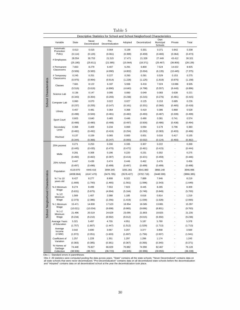
Table 5

Variable State NeverDecentralized

Pre­Decentralization Adopted Decentralized

OwnMunicipalSchools

Private Total

0.013 0.015 0.004 0.199 0.301 0.371 0.842 0.338

(0.114) (0.120) (0.061) (0.399) (0.459) (0.483) (0.364) (0.473)

28.554 30.753 21.515 17.471 21.328 27.449 43.412 30.321

(25.180) (25.811) (21.585) (15.564) (18.371) (25.467) (36.800) (28.139)

7.833 8.279 6.407 6.291 6.800 7.524 14.022 8.925

(5.506) (5.583) (4.990) (4.802) (5.004) (6.135) (10.445) (7.375)

0.245 0.251 0.227 0.293 0.281 0.529 0.153 0.275

(0.975) (0.994) (0.914) (1.228) (1.125) (1.819) (0.875) (1.158)

7.661 8.122 6.187 5.936 6.416 7.024 13.086 8.505

(5.516) (5.619) (4.890) (4.640) (4.798) (5.557) (9.440) (6.896)

0.136 0.147 0.095 0.060 0.049 0.083 0.638 0.221

(0.343) (0.354) (0.293) (0.238) (0.215) (0.276) (0.481) (0.415)

0.060 0.070 0.022 0.027 0.125 0.153 0.685 0.226

(0.237) (0.255) (0.147) (0.161) (0.331) (0.360) (0.465) (0.418)

0.457 0.481 0.364 0.368 0.419 0.386 0.868 0.528

(0.498) (0.500) (0.481) (0.482) (0.493) (0.487) (0.339) (0.499)

0.603 0.640 0.465 0.446 0.490 0.381 0.741 0.574

(0.489) (0.480) (0.499) (0.497) (0.500) (0.486) (0.438) (0.494)

0.368 0.409 0.234 0.069 0.094 0.179 0.796 0.383

(0.482) (0.492) (0.424) (0.254) (0.292) (0.383) (0.403) (0.486)

0.137 0.159 0.065 0.000 0.001 0.016 0.417 0.155

(0.344) (0.366) (0.247) (0.000) (0.032) (0.124) (0.493) (0.362)

0.271 0.253 0.330 0.335 0.307 0.222  ­ 0.269

(0.445) (0.435) (0.470) (0.472) (0.461) (0.415)  ­ (0.444)

0.281 0.308 0.196 0.220 0.231 0.302  ­ 0.275

(0.450) (0.462) (0.397) (0.414) (0.421) (0.459)  ­ (0.446)

0.447 0.439 0.474 0.446 0.462 0.476  ­ 0.456

(0.497) (0.496) (0.499) (0.497) (0.499) (0.499)  ­ (0.498)

4119.970 4440.416 3094.345 3291.361 3541.883 3866.148  ­ 3946.996

(4038.864) (4147.470) (3476.785) (3576.427) (3702.716) (3448.590)  ­ (3866.385)

8.427 8.277 8.908 8.322 7.889 7.946  ­ 8.219

(1.669) (1.700) (1.465) (1.561) (1.596) (1.543)  ­ (1.649)

8.274 8.499 7.553 7.923 8.445 8.265  ­ 8.309

(5.631) (5.875) (4.694) (5.164) (5.749) (5.849)  ­ (5.700)

1.569 1.407 2.088 1.185 0.616 0.814  ­ 1.219

(2.373) (2.386) (2.256) (1.419) (1.039) (1.628)  ­ (2.065)

15.471 14.830 17.523 16.954 16.585 13.881  ­ 15.397

(10.021) (10.034) (9.698) (9.965) (9.696) (8.801)  ­ (9.763)

21.496 20.519 24.629 23.095 21.803 19.825  ­ 21.235

(9.234) (9.210) (8.592) (9.012) (9.015) (9.350)  ­ (9.238)

5.321 5.497 4.755 4.951 5.187 5.760  ­ 5.378

(1.757) (1.807) (1.447) (1.512) (1.529) (1.713)  ­ (1.713)

3.542 3.690 3.067 3.207 3.377 3.858  ­ 3.569

(1.972) (2.051) (1.603) (1.697) (1.756) (2.007)  ­ (1.941)

1.257 1.228 1.351 1.297 1.266 1.174  ­ 1.243

(0.383) (0.385) (0.361) (0.367) (0.356) (0.340)  ­ (0.371)

74.448 76.827 66.829 70.882 74.990 82.467  ­ 76.128

(38.506) (38.741) (36.723) (34.845) (32.896) (30.855)  ­ (36.108)Obs 1 : Standard errors in parentheses

Descriptive Statistics for School and School Neigborhood Characteristics

Sch

ool C

hara

cter

istic

sS

choo

l Nei

gbor

hood

 Cha

ract

eris

tics

AutoimaticPromotion

Policy

# Employees

# PermanentClassrooms

# TemporaryClassrooms

Classes

Science Lab

Computer Lab

Library

Sport Court

SecondaryLevel

Hischool

% 1­2Minimum

Wage

Midle

25% richest

Population

% 7 to 10years old

25% poorest

% 0 MinimumWage

% 1/2Minimum

Wage

% 1 MinimumWage

% Homes w/GarbageCollection

Obs 2: All statistics were computed pooling the data across years. "State" contains all the state schools; "Never Decentralized" contains data onall state schools that were never decentralized; "Pre­Decentralization" contains data on all decentralized state schools before the decentralizationand "Adopted" contains data on all decentralized school at the year the decentralization took place.

Average Yearsof Education

AverageIncome(# MW)

Coefficient ofVariation

30

Table 6

State NeverDecentralized

Pre­Decentralization Adopted Decentralized Own Municipal

Schools Private Total

0.197 0.230 0.093 0.105 0.141 0.219 0.286 0.210(0.398) (0.421) (0.291) (0.307) (0.348) (0.414) (0.452) (0.407)0.367 0.351 0.421 0.446 0.397 0.330 0.324 0.357

(0.482) (0.477) (0.494) (0.497) (0.489) (0.470) (0.468) (0.479)0.436 0.420 0.486 0.448 0.462 0.451 0.390 0.433

(0.496) (0.494) (0.500) (0.497) (0.499) (0.498) (0.488) (0.495)21.026 20.617 22.336 21.203 21.908 20.303 18.661 20.562

(15.484) (14.925) (17.087) (13.521) (13.536) (12.810) (11.616) (14.056)

78.974 79.383 77.664 78.797 78.092 79.697 81.339 79.438

(15.484) (14.925) (17.087) (13.521) (13.536) (12.810) (11.616) (14.056)

28.505 27.635 31.289 27.153 27.817 26.548 25.140 27.375

(16.280) (15.412) (18.516) (13.851) (12.816) (12.720) (11.799) (14.398)

71.495 72.365 68.711 72.847 72.183 73.452 74.860 72.625

(16.280) (15.412) (18.516) (13.851) (12.816) (12.720) (11.799) (14.398)

4.458 4.616 3.952 4.013 3.813 4.409 4.851 4.425(1.900) (1.937) (1.680) (1.657) (1.554) (1.914) (1.881) (1.872)1.888 2.164 1.005 1.054 2.450 2.515 2.704 2.252

(2.561) (2.714) (1.719) (2.124) (2.761) (2.984) (3.040) (2.791)38.429 37.888 40.451 38.851 38.471 38.152 37.392 38.162

(19.958) (19.658) (20.920) (21.959) (21.615) (20.796) (19.936) (20.425)82.101 82.032 82.357 82.826 82.189 82.416 83.089 82.389(6.489) (6.458) (6.597) (5.799) (6.196) (5.324) (4.166) (5.811)0.333 0.333 0.336 0.382 0.463 0.410 0.349 0.370

(0.471) (0.471) (0.472) (0.486) (0.499) (0.492) (0.477) (0.483)185316.000 218059.800 80515.630 90372.260 98998.960 195258.100  ­ 168807.500

(258602.300) (279068.000) (131322.500) (137201.000) (142737.400) (265001.200)  ­ (242750.600)8.225 8.087 8.668 8.209 7.822 7.739  ­ 8.044

(1.095) (1.092) (0.981) (0.955) (0.978) (0.931)  ­ (1.063)8.615 8.515 8.933 8.649 8.431 8.309  ­ 8.516

(0.884) (0.871) (0.846) (0.822) (0.798) (0.784)  ­ (0.856)87.822 88.343 86.152 87.398 88.395 89.277  ­ 88.228(3.742) (3.681) (3.432) (3.166) (2.983) (3.077)  ­ (3.514)

5.750 5.914 5.222 5.476 5.692 6.155  ­ 5.816

(1.181) (1.183) (1.007) (0.994) (1.007) (1.136)  ­ (1.149)

3.924 4.061 3.486 3.671 3.837 4.267  ­ 3.972(1.317) (1.333) (1.157) (1.193) (1.245) (1.298)  ­ (1.307)1.187 1.164 1.260 1.226 1.197 1.130  ­ 1.178

(0.243) (0.239) (0.241) (0.227) (0.218) (0.196)  ­ (0.230)6614.595 6618.369 6602.518 6610.424 6534.614 5715.069  ­ 6422.283

(7194.749) (6954.447) (7915.480) (8301.605) (8572.034) (6935.624)  ­ (7470.692)15.203 13.121 21.865 19.147 16.850 10.722  ­ 14.682

(19.117) (17.797) (21.523) (19.799) (18.283) (14.146)  ­ (18.188)0.655 0.695 0.528 0.806 0.815 1.000  ­ 0.756

(0.475) (0.461) (0.499) (0.396) (0.388) (0.000)  ­ (0.429)0.300 0.333 0.193 0.227 0.252 0.228  ­ 0.276

(0.458) (0.471) (0.394) (0.419) (0.434) (0.419)  ­ (0.447)

Obs 1 : Standard errors in parentheses

Descriptive Statistics for the Municipalities Characteristics

Right Partymayor

% CityCouncil Gov.

# PartyCoalitions

Mayors'Voting Share

Turnout

Pol

itica

l Cha

ract

eris

tics

% CityCouncil

Oposotion toGov.

% CityCouncil Mayor

% CityCouncil

Oposition toMayor

# MayoralCandidates

Center Partymayor

Left Partymayor

Mayor alliedto the Gov

Population

% 7 to 10years old

% 11 to 14years old

Soc

al &

 Eco

nom

ic C

hara

cter

istic

s

Obs 2: All statistics were computed pooling the data across years. "State" contains all the state schools; "Never Decentralized" contains data on allstate schools that were never decentralized; "Pre­Decentralization" contains data on all decentralized state schools before the decentralization and"Adopted" contains data on all decentralized school at the year the decentralization took place.

RuralPopulation

% Rural Pop.

Own School

Own School1996

% Literacy

AverageYears of

Education

AverageIncome

Coefficient ofVariation

31

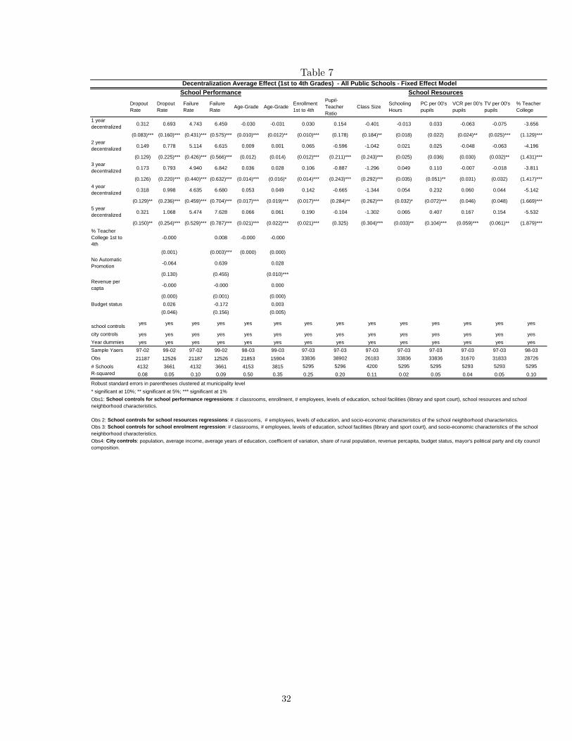
Table 7

DropoutRate

DropoutRate

FailureRate

FailureRate Age­Grade Age­Grade Enrollment

1st to 4th

Pupil­TeacherRatio

Class Size SchoolingHours

PC per 00'spupils

VCR per 00'spupils

TV per 00'spupils

% TeacherCollege

1 yeardecentralized 0.312 0.693 4.743 6.459 ­0.030 ­0.031 0.030 0.154 ­0.401 ­0.013 0.033 ­0.063 ­0.075 ­3.656

(0.083)*** (0.160)*** (0.431)*** (0.575)*** (0.010)*** (0.012)** (0.010)*** (0.178) (0.184)** (0.018) (0.022) (0.024)** (0.025)*** (1.129)***2 yeardecentralized 0.149 0.778 5.114 6.615 0.009 0.001 0.065 ­0.596 ­1.042 0.021 0.025 ­0.048 ­0.063 ­4.196

(0.129) (0.225)*** (0.426)*** (0.566)*** (0.012) (0.014) (0.012)*** (0.211)*** (0.243)*** (0.025) (0.036) (0.030) (0.032)** (1.431)***3 yeardecentralized 0.173 0.793 4.940 6.842 0.036 0.028 0.106 ­0.887 ­1.296 0.049 0.110 ­0.007 ­0.018 ­3.811

(0.126) (0.220)*** (0.440)*** (0.632)*** (0.014)*** (0.016)* (0.014)*** (0.243)*** (0.292)*** (0.035) (0.051)** (0.031) (0.032) (1.417)***4 yeardecentralized 0.318 0.998 4.635 6.680 0.053 0.049 0.142 ­0.665 ­1.344 0.054 0.232 0.060 0.044 ­5.142

(0.129)** (0.236)*** (0.459)*** (0.704)*** (0.017)*** (0.019)*** (0.017)*** (0.284)** (0.262)*** (0.032)* (0.072)*** (0.046) (0.048) (1.669)***5 yeardecentralized 0.321 1.068 5.474 7.628 0.066 0.061 0.190 ­0.104 ­1.302 0.065 0.407 0.167 0.154 ­5.532

(0.150)** (0.254)*** (0.529)*** (0.787)*** (0.021)*** (0.022)*** (0.021)*** (0.325) (0.304)*** (0.033)** (0.104)*** (0.059)*** (0.061)** (1.879)***% TeacherCollege 1st to4th

­0.000 0.008 ­0.000 ­0.000

(0.001) (0.003)*** (0.000) (0.000)No AutomaticPromotion ­0.064 0.639 0.028

(0.130) (0.455) (0.010)***Revenue percapta ­0.000 ­0.000 0.000

(0.000) (0.001) (0.000)Budget status 0.026 ­0.172 0.003

(0.046) (0.156) (0.005)

school controls yes yes yes yes yes yes yes yes yes yes yes yes yes yes

city controls yes yes yes yes yes yes yes yes yes yes yes yes yes yesYear dummies yes yes yes yes yes yes yes yes yes yes yes yes yes yesSample Yaers 97­02 99­02 97­02 99­02 98­03 99­03 97­03 97­03 97­03 97­03 97­03 97­03 97­03 98­03Obs 21187 12526 21187 12526 21853 15904 33836 38902 26183 33836 33836 31670 31833 28726# Schools 4132 3661 4132 3661 4153 3815 5295 5296 4200 5295 5295 5293 5293 5295R­squared 0.08 0.05 0.10 0.09 0.50 0.35 0.25 0.20 0.11 0.02 0.05 0.04 0.05 0.10

Robust standard errors in parentheses clustered at municipality level* significant at 10%; ** significant at 5%; *** significant at 1%

Obs 2: School controls for school resources regressions: # classrooms,  # employees, levels of education, and socio­economic characteristics of the school neighborhood characteristics.Obs 3: School controls for school enrolment regression: # classrooms, # employees, levels of education, school facilities (library and sport court), and socio­economic characteristics of the schoolneighborhood characteristics.Obs4: City controls: population, average income, average years of education, coefficient of variation, share of rural population, revenue percapita, budget status, mayor's political party and city councilcomposition.

 Decentralization Average Effect (1st to 4th Grades)  ­ All Public Schools ­ Fixed Effect ModelSchool Performance School Resources

Obs1: School controls for school performance regressions: # classrooms, enrollment, # employees, levels of education, school facilities (library and sport court), school resources and schoolneighborhood characteristics.

32

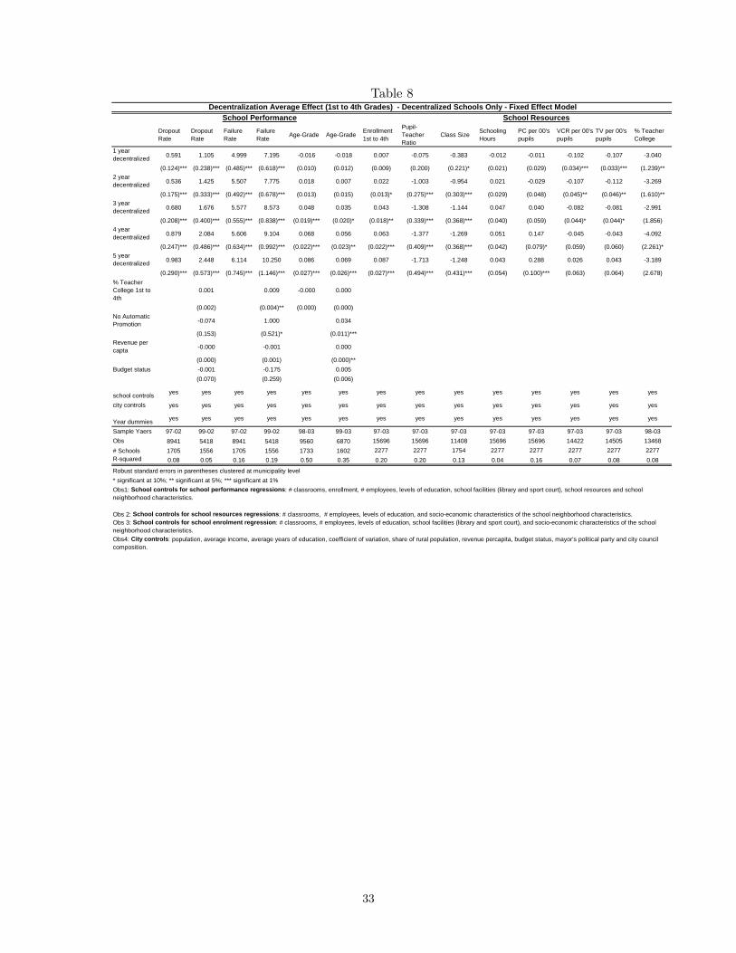
Table 8

DropoutRate

DropoutRate

FailureRate

FailureRate Age­Grade Age­Grade Enrollment

1st to 4th

Pupil­TeacherRatio

Class Size SchoolingHours

PC per 00'spupils

VCR per 00'spupils

TV per 00'spupils

% TeacherCollege

1 yeardecentralized 0.591 1.105 4.999 7.195 ­0.016 ­0.018 0.007 ­0.075 ­0.383 ­0.012 ­0.011 ­0.102 ­0.107 ­3.040

(0.124)*** (0.238)*** (0.485)*** (0.618)*** (0.010) (0.012) (0.009) (0.200) (0.221)* (0.021) (0.029) (0.034)*** (0.033)*** (1.239)**2 yeardecentralized 0.536 1.425 5.507 7.775 0.018 0.007 0.022 ­1.003 ­0.954 0.021 ­0.029 ­0.107 ­0.112 ­3.269

(0.175)*** (0.333)*** (0.492)*** (0.678)*** (0.013) (0.015) (0.013)* (0.275)*** (0.303)*** (0.029) (0.048) (0.045)** (0.046)** (1.610)**3 yeardecentralized 0.680 1.676 5.577 8.573 0.048 0.035 0.043 ­1.308 ­1.144 0.047 0.040 ­0.082 ­0.081 ­2.991

(0.208)*** (0.400)*** (0.555)*** (0.838)*** (0.019)*** (0.020)* (0.018)** (0.339)*** (0.368)*** (0.040) (0.059) (0.044)* (0.044)* (1.856)4 yeardecentralized 0.879 2.084 5.606 9.104 0.068 0.056 0.063 ­1.377 ­1.269 0.051 0.147 ­0.045 ­0.043 ­4.092

(0.247)*** (0.486)*** (0.634)*** (0.992)*** (0.022)*** (0.023)** (0.022)*** (0.409)*** (0.368)*** (0.042) (0.079)* (0.059) (0.060) (2.261)*5 yeardecentralized 0.983 2.448 6.114 10.250 0.086 0.069 0.087 ­1.713 ­1.248 0.043 0.288 0.026 0.043 ­3.189

(0.290)*** (0.573)*** (0.745)*** (1.146)*** (0.027)*** (0.026)*** (0.027)*** (0.494)*** (0.431)*** (0.054) (0.100)*** (0.063) (0.064) (2.678)% TeacherCollege 1st to4th

0.001 0.009 ­0.000 0.000

(0.002) (0.004)** (0.000) (0.000)No AutomaticPromotion ­0.074 1.000 0.034

(0.153) (0.521)* (0.011)***Revenue percapta ­0.000 ­0.001 0.000

(0.000) (0.001) (0.000)**Budget status ­0.001 ­0.175 0.005

(0.070) (0.259) (0.006)

school controls yes yes yes yes yes yes yes yes yes yes yes yes yes yes

city controls yes yes yes yes yes yes yes yes yes yes yes yes yes yes

Year dummies yes yes yes yes yes yes yes yes yes yes yes yes yes yes

Sample Yaers 97­02 99­02 97­02 99­02 98­03 99­03 97­03 97­03 97­03 97­03 97­03 97­03 97­03 98­03Obs 8941 5418 8941 5418 9560 6870 15696 15696 11408 15696 15696 14422 14505 13468# Schools 1705 1556 1705 1556 1733 1602 2277 2277 1754 2277 2277 2277 2277 2277R­squared 0.08 0.05 0.16 0.19 0.50 0.35 0.20 0.20 0.13 0.04 0.16 0.07 0.08 0.08

Robust standard errors in parentheses clustered at municipality level* significant at 10%; ** significant at 5%; *** significant at 1%

 Decentralization Average Effect (1st to 4th Grades)  ­ Decentralized Schools Only ­ Fixed Effect ModelSchool Performance School Resources

Obs1: School controls for school performance regressions: # classrooms, enrollment, # employees, levels of education, school facilities (library and sport court), school resources and schoolneighborhood characteristics.

Obs 2: School controls for school resources regressions: # classrooms,  # employees, levels of education, and socio­economic characteristics of the school neighborhood characteristics.Obs 3: School controls for school enrolment regression: # classrooms, # employees, levels of education, school facilities (library and sport court), and socio­economic characteristics of the schoolneighborhood characteristics.Obs4: City controls: population, average income, average years of education, coefficient of variation, share of rural population, revenue percapita, budget status, mayor's political party and city councilcomposition.

33

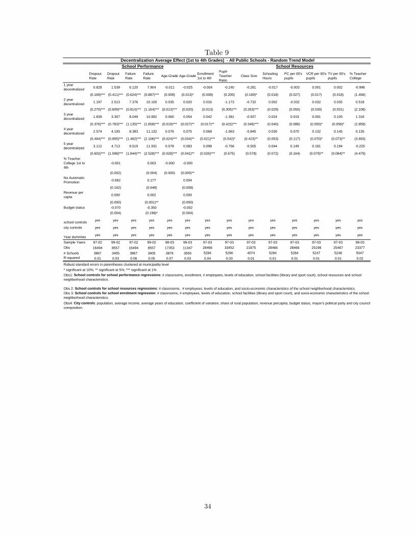
Table 9

DropoutRate

DropoutRate

FailureRate

FailureRate Age­Grade Age­Grade Enrollment

1st to 4th

Pupil­TeacherRatio

Class Size SchoolingHours

PC per 00'spupils

VCR per 00'spupils

TV per 00'spupils

% TeacherCollege

1 yeardecentralized 0.828 1.539 6.120 7.904 ­0.011 ­0.025 ­0.004 ­0.240 ­0.281 ­0.017 ­0.003 0.001 0.002 ­0.996

(0.169)*** (0.411)*** (0.624)*** (0.887)*** (0.009) (0.013)* (0.008) (0.200) (0.169)* (0.018) (0.027) (0.017) (0.018) (1.456)2 yeardecentralized 1.197 2.513 7.376 10.100 0.035 0.020 0.016 ­1.173 ­0.732 0.002 ­0.032 0.032 0.035 0.518

(0.270)*** (0.609)*** (0.814)*** (1.164)*** (0.013)*** (0.020) (0.013) (0.305)*** (0.263)*** (0.029) (0.055) (0.030) (0.031) (2.108)3 yeardecentralized 1.839 3.307 8.049 10.992 0.060 0.054 0.042 ­1.381 ­0.937 0.024 0.019 0.091 0.105 1.316

(0.376)*** (0.783)*** (1.135)*** (1.658)*** (0.019)*** (0.027)** (0.017)** (0.415)*** (0.346)*** (0.040) (0.086) (0.055)* (0.056)* (2.858)4 yeardecentralized 2.574 4.193 8.383 11.132 0.076 0.075 0.068 ­1.063 ­0.845 0.030 0.070 0.132 0.145 0.135

(0.494)*** (0.955)*** (1.482)*** (2.106)*** (0.024)*** (0.034)** (0.021)*** (0.542)* (0.423)** (0.053) (0.117) (0.070)* (0.073)** (3.693)5 yeardecentralized 3.112 4.713 9.519 11.931 0.078 0.083 0.098 ­0.756 ­0.505 0.044 0.149 0.181 0.194 ­0.225

(0.602)*** (1.098)*** (1.844)*** (2.528)*** (0.028)*** (0.041)** (0.026)*** (0.675) (0.578) (0.072) (0.164) (0.079)** (0.084)** (4.479)% TeacherCollege 1st to4th

­0.001 0.003 ­0.000 ­0.000

(0.002) (0.004) (0.000) (0.000)**No AutomaticPromotion ­0.062 0.177 0.004

(0.162) (0.648) (0.008)Revenue percapta 0.000 0.002 0.000

(0.000) (0.001)** (0.000)Budget status ­0.070 ­0.350 ­0.002

(0.054) (0.198)* (0.004)

school controls yes yes yes yes yes yes yes yes yes yes yes yes yes yes

city controls yes yes yes yes yes yes yes yes yes yes yes yes yes yes

Year dummies yes yes yes yes yes yes yes yes yes yes yes yes yes yes

Sample Yaers 97­02 99­02 97­02 99­02 98­03 99­03 97­03 97­03 97­03 97­03 97­03 97­03 97­03 98­03Obs 16494 8557 16494 8557 17353 11347 28466 33452 21875 28466 28466 25198 25467 23377# Schools 3867 3405 3867 3405 3876 3555 5284 5290 4074 5284 5284 5247 5248 5047R­squared 0.01 0.03 0.06 0.05 0.07 0.03 0.04 0.03 0.01 0.01 0.01 0.01 0.01 0.02

Robust standard errors in parentheses clustered at municipality level* significant at 10%; ** significant at 5%; *** significant at 1%

Obs4: City controls: population, average income, average years of education, coefficient of variation, share of rural population, revenue percapita, budget status, mayor's political party and city councilcomposition.

Obs 3: School controls for school enrolment regression: # classrooms, # employees, levels of education, school facilities (library and sport court), and socio­economic characteristics of the schoolneighborhood characteristics.

Obs1: School controls for school performance regressions: # classrooms, enrollment, # employees, levels of education, school facilities (library and sport court), school resources and schoolneighborhood characteristics.

 Decentralization Average Effect (1st to 4th Grades)  ­ All Public Schools ­ Random Trend ModelSchool Performance School Resources

Obs 2: School controls for school resources regressions: # classrooms,  # employees, levels of education, and socio­economic characteristics of the school neighborhood characteristics.

34

Table 10

DropoutRate

DropoutRate

FailureRate

FailureRate Age­Grade Age­Grade Enrollment

1st to 4th

Pupil­TeacherRatio

Class Size SchoolingHours

PC per 00'spupils

VCR per 00'spupils

TV per 00'spupils

% TeacherCollege

1 yeardecentralized 0.863 1.575 5.917 7.944 ­0.003 ­0.016 ­0.001 ­0.087 ­0.272 ­0.008 0.004 ­0.000 ­0.001 ­1.973

(0.174)*** (0.406)*** (0.630)*** (0.840)*** (0.009) (0.012) (0.009) (0.200) (0.171) (0.018) (0.025) (0.017) (0.018) (1.464)2 yeardecentralized 1.219 2.600 7.404 10.773 0.041 0.029 0.016 ­0.987 ­0.745 0.019 ­0.021 0.022 0.021 ­1.388

(0.272)*** (0.629)*** (0.823)*** (1.144)*** (0.013)*** (0.019) (0.014) (0.300)*** (0.263)*** (0.029) (0.054) (0.030) (0.033) (2.053)3 yeardecentralized 1.829 3.409 8.369 12.390 0.071 0.068 0.034 ­1.187 ­1.016 0.048 0.021 0.074 0.084 ­1.810

(0.377)*** (0.823)*** (1.139)*** (1.623)*** (0.019)*** (0.026)*** (0.018)* (0.403)*** (0.341)*** (0.040) (0.084) (0.055) (0.057) (2.796)4 yeardecentralized 2.462 4.235 8.939 12.991 0.091 0.090 0.048 ­1.141 ­1.126 0.064 0.061 0.103 0.113 ­3.963

(0.486)*** (0.994)*** (1.480)*** (2.033)*** (0.025)*** (0.033)*** (0.023)** (0.510)** (0.428)*** (0.055) (0.115) (0.074) (0.078) (3.692)5 yeardecentralized 2.873 4.681 9.270 13.266 0.101 0.099 0.062 ­1.278 ­0.941 0.083 0.108 0.148 0.163 ­5.088

(0.593)*** (1.127)*** (1.813)*** (2.347)*** (0.030)*** (0.039)** (0.028)** (0.617)** (0.579) (0.074) (0.164) (0.085)* (0.092)* (4.439)% TeacherCollege 1st to4th

0.004 0.000 ­0.000 ­0.000

(0.003) (0.005) (0.000) (0.000)**Automaticpromotion 0.027 0.871 0.001

(0.178) (0.613) (0.009)Revenue percapta 0.000 0.002 ­0.000

(0.000) (0.001)* (0.000)***Budget status ­0.147 ­0.248 0.004

(0.098) (0.240) (0.005)

school controls yes yes yes yes yes yes yes yes yes yes yes yes yes yes

city controls yes yes yes yes yes yes yes yes yes yes yes yes yes yes

Year dummies yes yes yes yes yes yes yes yes yes yes yes yes yes yes

Sample Yaers 97­02 99­02 97­02 99­02 98­03 99­03 97­03 97­03 97­03 97­03 97­03 97­03 97­03 98­03Obs 6757 3778 6757 3778 7617 4939 13385 15559 9584 13385 13385 11432 11570 11165# Schools 1637 1480 1637 1480 1645 1500 2277 2277 1680 2277 2277 2262 2263 2275R­squared 0.02 0.04 0.10 0.16 0.08 0.05 0.06 0.02 0.01 0.02 0.02 0.01 0.01 0.01

Robust standard errors in parentheses clustered at municipality level* significant at 10%; ** significant at 5%; *** significant at 1%

Obs 2: School controls for school resources regressions: # classrooms,  # employees, levels of education, and socio­economic characteristics of the school neighborhood characteristics.Obs 3: School controls for school enrolment regression: # classrooms, # employees, levels of education, school facilities (library and sport court), and socio­economic characteristics of the schoolneighborhood characteristics.Obs4: City controls: population, average income, average years of education, coefficient of variation, share of rural population, revenue percapita, budget status, mayor's political party and city councilcomposition.

 Decentralization Average Effect (1st to 4th Grades)  ­ Decentralized Schools Only ­ Random Trend ModelSchool Performance School Resources

Obs1: School controls for school performance regressions: # classrooms, enrollment, # employees, levels of education, school facilities (library and sport court), school resources and schoolneighborhood characteristics.

35

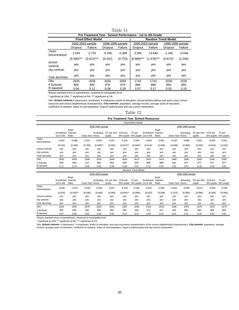
Table 11

Dropout Failure Dropout Failure Dropout Failure Dropout FailureYearsDecentralized 1.544 2.733 ­0.436 ­0.368 3.395 13.840 ­1.160 ­0.048

(0.380)*** (0.812)*** (0.422) (0.753) (0.886)*** (1.978)*** (0.672)* (1.246)schoolcontrols yes yes yes yes yes yes yes yes

city controls yes yes yes yes yes yes yes yes

Year dummies yes yes yes yes yes yes yes yes

Obs 2635 2635 3092 3092 1743 1743 2035 2035# Schools 892 892 876 876 884 884 855 855R­squared 0.04 0.12 0.09 0.29 0.07 0.17 0.03 0.15Robust standard errors in parentheses, clustered at municipality level* significant at 10%; ** significant at 5%; *** significant at 1%Obs: School controls:# classrooms, enrollment, # employees, levels of education, school facilities (library and sport court), schoolresources and school neighborhood characteristics. City controls: population, average income, average years of education,coefficient of variation, share of rural population, mayor's political party and city council composition.

Random Trend Model2000­2003 sample 1996­1999 sample

 Pre Treatment Test ­ School Performance ­ 1st to 4th Grade

2000­2003 sample 1996­1999 sampleFixed Effect Model

Table 12

Enrollment1st to 4th

Pupil­TeacherRatio Class Size

SchoolingHours

PC per 00'spupils

VCR per00's pupils

TV per00's pupils

Enrollment1st to 4th

Pupil­TeacherRatio Class Size

SchoolingHours

PC per 00'spupils

VCR per00's pupils

TV per00's pupils

YearsDecentralized ­0.001 ­0.486 0.224 0.085 0.041 0.105 0.094 ­0.024 0.081 ­0.197 ­0.080 0.021 ­0.022 0.010

(0.016) (0.295) (0.283) (0.039)** (0.062) (0.047)** (0.046)** (0.014)* (0.269) (0.698) (0.059) (0.020) (0.024) (0.026)school controls yes yes yes yes yes yes yes yes yes yes yes yes yes yescity controls yes yes yes yes yes yes yes yes yes yes yes yes yes yesYear dummies yes yes yes yes yes yes yes yes yes yes yes yes yes yesObs 3530 3530 2299 3530 3530 2844 2873 3415 3415 1680 2560 2560 2560 2560# Schools 893 893 612 893 893 893 893 888 888 591 877 877 877 877R­squared 0.11 0.14 0.09 0.05 0.08 0.08 0.07 0.12 0.04 0.01 0.01 0.18 0.03 0.03

Enrollment1st to 4th

Pupil­TeacherRatio Class Size

SchoolingHours

PC per 00'spupils

VCR per00's pupils

TV per00's pupils

Enrollment1st to 4th

Pupil­TeacherRatio Class Size

SchoolingHours

PC per 00'spupils

VCR per00's pupils

TV per00's pupils

YearsDecentralized ­0.028 ­1.223 ­0.050 ­0.055 0.027 0.129 0.108 ­0.015 0.209 0.563 ­0.090 ­0.013 ­0.050 ­0.030

(0.019) (0.502)** (0.430) (0.050) (0.083) (0.054)** (0.056)* (0.022) (0.568) (1.210) (0.083) (0.056) (0.055) (0.056)school controls yes yes yes yes yes yes yes yes yes yes yes yes yes yescity controls yes yes yes yes yes yes yes yes yes yes yes yes yes yesYear dummies yes yes yes yes yes yes yes yes yes yes yes yes yes yesObs 2634 2634 1679 2634 2634 1587 1636 2516 2516 1085 1679 1679 1679 1679# Schools 892 892 582 892 892 584 593 871 871 555 860 860 860 860R­squared 0.07 0.05 0.02 0.03 0.02 0.14 0.14 0.05 0.01 0.01 0.01 0.29 0.02 0.01

Robust standard errors in parentheses, clustered at municipality level* significant at 10%; ** significant at 5%; *** significant at 1%

2000­2003 sample 1996­1999 sample

 Pre Treatment Test ­School Resources

Obs: School controls: # classrooms,  # employees, levels of education, and socio­economic characteristics of the school neighborhood characteristics. City controls: population, averageincome, average years of education, coefficient of variation, share of rural population, mayor's political party and city council composition.

2000­2003 sample 1996­1999 sample

Fixed Effect Model

 Random Trend Model

36

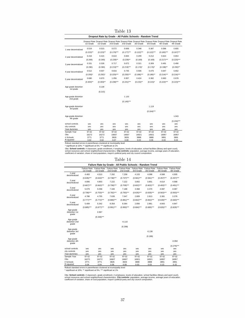
Table 13

Dropout Rate1st Grade

Dropout Rate1st Grade

Dropout Rate2nd Grade

Dropout Rate2nd Grade

Dropout Rate3rd Grade

Dropout Rate3rd Grade

Dropout Rate4th Grade

Dropout Rate4th Grade

1 year decentralized 0.519 0.523 0.572 0.606 0.348 0.387 0.586 0.655

(0.223)** (0.223)** (0.179)*** (0.177)*** (0.122)*** (0.122)*** (0.165)*** (0.167)***

2 year decentralized 0.416 0.415 0.610 0.604 0.209 0.212 0.624 0.654

(0.269) (0.269) (0.239)** (0.239)** (0.169) (0.169) (0.217)*** (0.220)***

3 year decentralized 0.331 0.328 0.717 0.672 0.321 0.309 0.491 0.490

(0.280) (0.280) (0.219)*** (0.219)*** (0.176)* (0.176)* (0.198)** (0.200)**

4 year decentralized 0.512 0.507 0.816 0.735 0.506 0.475 0.647 0.652

(0.293)* (0.292)* (0.229)*** (0.230)*** (0.186)*** (0.186)** (0.214)*** (0.216)***

5 year decentralized 0.680 0.670 1.056 0.957 0.424 0.382 0.683 0.678

(0.304)** (0.303)** (0.238)*** (0.241)*** (0.215)** (0.215)* (0.223)*** (0.223)***

Age­grade distortion1st grade

0.139

(0.215)

Age­grade distortion2nd grade

1.120

(0.140)***

Age­grade distortion3rd grade

1.119

(0.164)***

Age­grade distortion4th grade

1.043

(0.150)***school controls yes yes yes yes yes yes yes yescity controls yes yes yes yes yes yes yes yesYear dummies yes yes yes yes yes yes yes yesSample Year 97­02 97­02 97­02 97­02 97­02 97­02 97­02 97­02Obs 16272 16272 16607 16607 16921 16921 16957 16957# Schools 3771 3771 3826 3826 3888 3888 3891 3891R­squared 0.02 0.02 0.07 0.08 0.03 0.05 0.03 0.04Robust standard errors in parentheses clustered at municipality level* significant at 10%; ** significant at 5%; *** significant at 1%

Dropout Rate by Grade ­ All Public Schools ­ Random Trend

Obs: School controls: # classroom, grade enrollment, # employees, levels of education, school facilities (library and sport court),school resources and school neighborhood characteristics. City controls: population, average income, average years of education,coefficient of variation, share of rural population, mayor's political party and city council composition.

Table 14

Failure Rate1st Grade

Failure Rate1st Grade

Failure Rate2nd Grade

Failure Rate2nd Grade

Failure Rate3rd Grade

Failure Rate3rd Grade

Failure Rate4th Grade

Failure Rate4th Grade

1 yeardecentralized 4.483 4.510 7.262 7.258 4.103 4.098 4.568 4.505

(0.635)*** (0.633)*** (0.738)*** (0.737)*** (0.581)*** (0.581)*** (0.457)*** (0.457)***2 year

decentralized 4.806 4.803 7.222 7.222 3.802 3.801 4.614 4.588

(0.667)*** (0.663)*** (0.708)*** (0.709)*** (0.602)*** (0.602)*** (0.493)*** (0.491)***3 year

decentralized 5.079 5.058 7.184 7.188 3.368 3.370 4.087 4.087

(0.708)*** (0.703)*** (0.782)*** (0.783)*** (0.635)*** (0.635)*** (0.563)*** (0.563)***4 year

decentralized 4.788 4.755 7.639 7.647 2.809 2.813 3.381 3.378

(0.777)*** (0.772)*** (0.880)*** (0.881)*** (0.662)*** (0.662)*** (0.639)*** (0.640)***5 year

decentralized 5.409 5.342 8.354 8.364 2.856 2.861 4.843 4.847

(0.885)*** (0.877)*** (0.991)*** (0.993)*** (0.684)*** (0.685)*** (0.826)*** (0.829)***Age­grade

distortion 1stgrade

0.967

(0.336)***Age­grade

distortion 2ndgrade

­0.110

(0.298)Age­grade

distortion 3rdgrade

­0.136

(0.186)Age­grade

distortion 4thgrade

­0.950

(0.279)***school controls yes yes yes yes yes yes yes yescity controls yes yes yes yes yes yes yes yesYear dummies yes yes yes yes yes yes yes yesSample Year 97­02 97­02 97­02 97­02 97­02 97­02 97­02 97­02Obs 16272 16272 16607 16607 16921 16921 16957 16957# Schools 3771 3771 3826 3826 3888 3888 3891 3891R­squared 0.04 0.04 0.06 0.06 0.03 0.03 0.15 0.15Robust standard errors in parentheses clustered at municipality level* significant at 10%; ** significant at 5%; *** significant at 1%

Failure Rate by Grade ­ All Public Schools ­ Random Trend

Obs: School controls: # classroom, grade enrollment, # employees, levels of education, school facilities (library and sport court),school resources and school neighborhood characteristics. City controls: population, average income, average years of education,coefficient of variation, share of rural population, mayor's political party and city council composition.

37

Table 15

Age­GradeDistortion 1st

Grade

Age­GradeDistortion 1st

Grade

Age­GradeDistortion2nd Grade

Age­GradeDistortion2nd Grade

Age­GradeDistortion 3rd

Grade

Age­GradeDistortion 3rd

Grade

Age­GradeDistortion 4th

Grade

Age­GradeDistortion 4th

Grade1 year

decentralized ­0.017 ­0.017 0.018 0.018 ­0.017 ­0.017 ­0.021 ­0.023

(0.013) (0.013) (0.016) (0.016) (0.017) (0.017) (0.017) (0.017)2 year

decentralized 0.039 0.038 0.081 0.079 ­0.009 ­0.009 0.020 0.015

(0.022)* (0.022)* (0.028)*** (0.027)*** (0.028) (0.028) (0.026) (0.026)3 year

decentralized 0.063 0.062 0.120 0.118 ­0.035 ­0.039 0.027 0.019

(0.031)** (0.031)** (0.039)*** (0.038)*** (0.040) (0.039) (0.039) (0.039)4 year

decentralized 0.084 0.083 0.150 0.149 ­0.055 ­0.059 0.014 0.001

(0.041)** (0.041)** (0.052)*** (0.051)*** (0.053) (0.053) (0.053) (0.054)5 year

decentralized 0.117 0.116 0.145 0.145 ­0.090 ­0.096 0.001 ­0.015

(0.052)** (0.053)** (0.064)** (0.063)** (0.066) (0.066) (0.068) (0.069)Log Enrollment

1st grade 0.004

(0.009)Log Enrollment

2nd grade 0.067

(0.011)***Log Enrollment

3rd grade 0.085

(0.013)***Log Enrollment

4th grade 0.056

(0.017)***school controls yes yes yes yes yes yes yes yescity controls yes yes yes yes yes yes yes yesYear dummies yes yes yes yes yes yes yes yesSample Year 98­03 98­03 98­03 98­03 98­03 98­03 98­03 98­03Obs 12983 12983 13302 13302 13588 13588 13867 13867# Schools 3602 3602 3675 3675 3743 3743 3817 3817R­squared 0.02 0.02 0.05 0.05 0.01 0.02 0.06 0.06Robust standard errors in parentheses clustered at municipality level* significant at 10%; ** significant at 5%; *** significant at 1%

Age­Grade Distortion by Grade ­ All Public Schools ­ Random Trend

Obs: School controls: # classroom, grade enrollment, # employees, levels of education, school facilities (library and sport court),school resources and school neighborhood characteristics. City controls: population, average income, average years of education,coefficient of variation, share of rural population, mayor's political party and city council composition.

38

Table 16

Enrollment1st Grade

Enrollment2nd Grade

Enrollment3rd Grade

Enrollment4th Grade

1 yeardecentralized 4.222 2.448 ­1.641 ­1.843

(1.351)*** (1.156)** (0.995)* (1.100)*2 yeardecentralized 7.361 7.871 ­2.106 ­4.318

(2.045)*** (2.284)*** (1.278)* (1.535)***3 yeardecentralized 6.602 9.712 0.751 ­4.511

(2.449)*** (2.965)*** (1.924) (2.120)**4 yeardecentralized 6.442 10.188 1.258 ­2.005

(3.226)** (3.755)*** (2.408) (2.658)5 yeardecentralized 7.241 10.059 2.338 ­1.652

(4.026)* (4.629)** (3.516) (3.266)

school controls yes yes yes yes

city controls yes yes yes yesYear dummies yes yes yes yesSample Year 98­03 98­03 98­03 98­03Obs 26677 27284 27614 27821# Schools 5054 5142 5196 5238R­squared 0.04 0.11 0.07 0.06

Robust standard errors in parentheses clustered at municipality level* significant at 10%; ** significant at 5%; *** significant at 1%

School Enrollment by Grade ­ All Public Schools ­Random Trend Model

Obs 2: School controls: # classroom, # employees, levels of education,school facilities (library, science and computer lab, and  sport court),grade level schooling hours, % college educated teachers, and schoolneighborhood characteristics.

Obs3: City controls: population, average income, average years ofeducation, coefficient of variation, share of rural population, mayor'spolitical party and city council composition.

Obs 1: Enrollment is given by # students enrolled

39

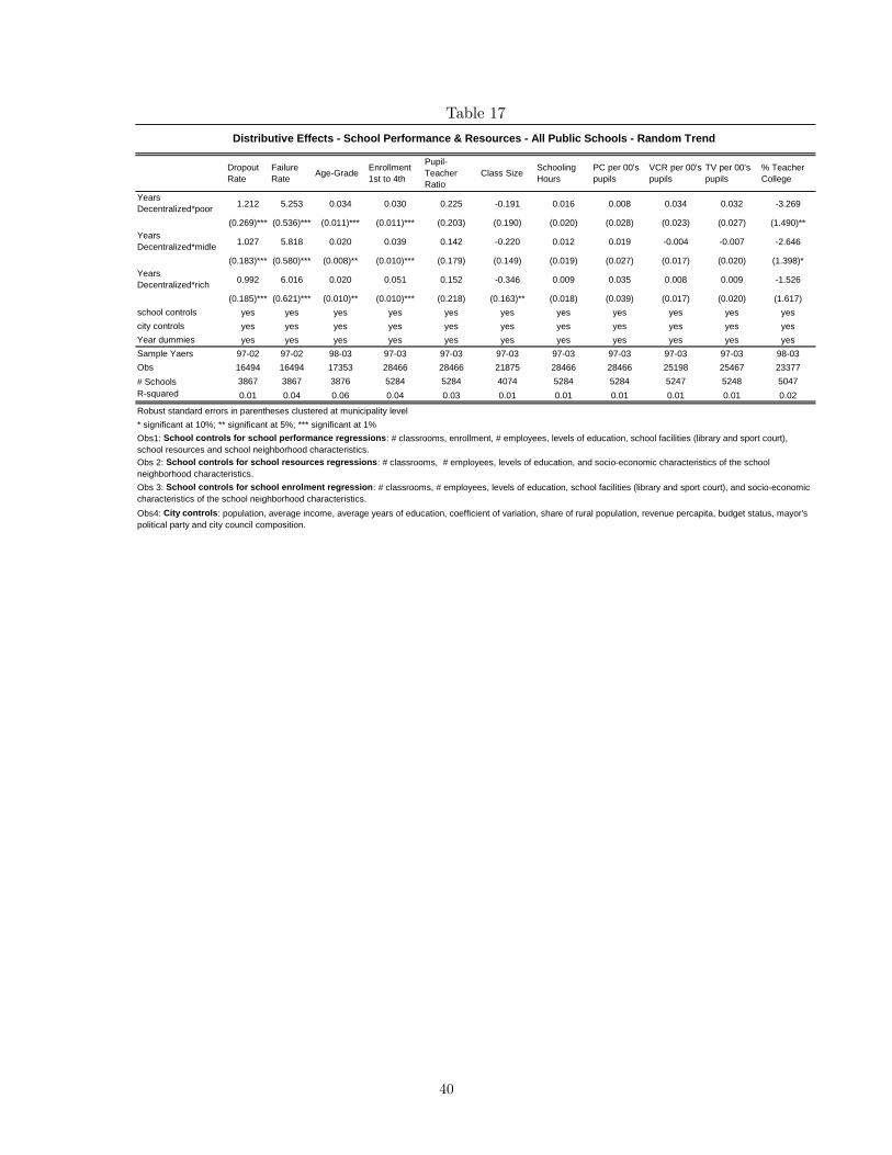
Table 17

DropoutRate

FailureRate Age­Grade Enrollment

1st to 4th

Pupil­TeacherRatio

Class Size SchoolingHours

PC per 00'spupils

VCR per 00'spupils

TV per 00'spupils

% TeacherCollege

YearsDecentralized*poor 1.212 5.253 0.034 0.030 0.225 ­0.191 0.016 0.008 0.034 0.032 ­3.269

(0.269)*** (0.536)*** (0.011)*** (0.011)*** (0.203) (0.190) (0.020) (0.028) (0.023) (0.027) (1.490)**YearsDecentralized*midle 1.027 5.818 0.020 0.039 0.142 ­0.220 0.012 0.019 ­0.004 ­0.007 ­2.646

(0.183)*** (0.580)*** (0.008)** (0.010)*** (0.179) (0.149) (0.019) (0.027) (0.017) (0.020) (1.398)*YearsDecentralized*rich 0.992 6.016 0.020 0.051 0.152 ­0.346 0.009 0.035 0.008 0.009 ­1.526

(0.185)*** (0.621)*** (0.010)** (0.010)*** (0.218) (0.163)** (0.018) (0.039) (0.017) (0.020) (1.617)school controls yes yes yes yes yes yes yes yes yes yes yescity controls yes yes yes yes yes yes yes yes yes yes yesYear dummies yes yes yes yes yes yes yes yes yes yes yesSample Yaers 97­02 97­02 98­03 97­03 97­03 97­03 97­03 97­03 97­03 97­03 98­03Obs 16494 16494 17353 28466 28466 21875 28466 28466 25198 25467 23377# Schools 3867 3867 3876 5284 5284 4074 5284 5284 5247 5248 5047R­squared 0.01 0.04 0.06 0.04 0.03 0.01 0.01 0.01 0.01 0.01 0.02

Robust standard errors in parentheses clustered at municipality level* significant at 10%; ** significant at 5%; *** significant at 1%

Obs 2: School controls for school resources regressions: # classrooms,  # employees, levels of education, and socio­economic characteristics of the schoolneighborhood characteristics.Obs 3: School controls for school enrolment regression: # classrooms, # employees, levels of education, school facilities (library and sport court), and socio­economiccharacteristics of the school neighborhood characteristics.Obs4: City controls: population, average income, average years of education, coefficient of variation, share of rural population, revenue percapita, budget status, mayor'spolitical party and city council composition.

Distributive Effects ­ School Performance & Resources ­ All Public Schools ­ Random Trend

Obs1: School controls for school performance regressions: # classrooms, enrollment, # employees, levels of education, school facilities (library and sport court),school resources and school neighborhood characteristics.

40

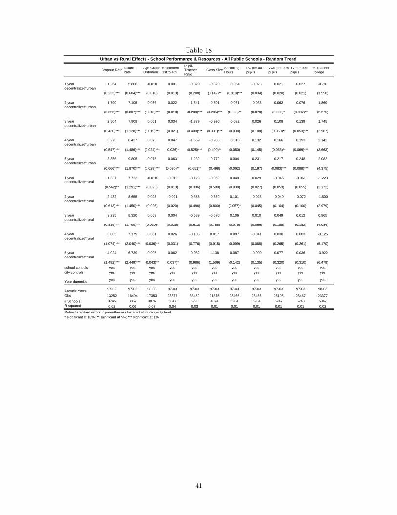
Table 18

Dropout Rate FailureRate

Age­GradeDistortion

Enrollment1st to 4th

Pupil­TeacherRatio

Class Size SchoolingHours

PC per 00'spupils

VCR per 00'spupils

TV per 00'spupils

% TeacherCollege

1 yeardecentralized*urban

1.264 5.806 ­0.010 0.001 ­0.320 ­0.320 ­0.054 ­0.023 0.021 0.027 ­0.781

(0.233)*** (0.604)*** (0.010) (0.013) (0.208) (0.149)** (0.018)*** (0.034) (0.020) (0.021) (1.550)

2 yeardecentralized*urban

1.790 7.105 0.036 0.022 ­1.541 ­0.801 ­0.061 ­0.036 0.062 0.076 1.869

(0.323)*** (0.807)*** (0.013)*** (0.018) (0.288)*** (0.235)*** (0.028)** (0.070) (0.035)* (0.037)** (2.275)

3 yeardecentralized*urban

2.504 7.908 0.061 0.034 ­1.879 ­0.990 ­0.032 0.026 0.108 0.139 1.745

(0.430)*** (1.128)*** (0.019)*** (0.021) (0.400)*** (0.331)*** (0.038) (0.108) (0.050)** (0.053)*** (2.967)

4 yeardecentralized*urban

3.273 8.437 0.075 0.047 ­1.659 ­0.988 ­0.018 0.132 0.166 0.193 2.142

(0.547)*** (1.486)*** (0.024)*** (0.026)* (0.525)*** (0.400)** (0.050) (0.145) (0.065)** (0.069)*** (3.663)

5 yeardecentralized*urban

3.856 9.805 0.075 0.063 ­1.232 ­0.772 0.004 0.231 0.217 0.248 2.082

(0.666)*** (1.870)*** (0.029)*** (0.030)** (0.651)* (0.498) (0.062) (0.197) (0.083)*** (0.088)*** (4.375)

1 yeardecentralized*rural

1.337 7.723 ­0.018 ­0.019 ­0.123 ­0.069 0.040 0.029 ­0.045 ­0.061 ­1.223

(0.562)** (1.291)*** (0.025) (0.013) (0.336) (0.590) (0.038) (0.027) (0.053) (0.055) (2.172)

2 yeardecentralized*rural

2.432 8.655 0.023 ­0.021 ­0.585 ­0.369 0.101 ­0.023 ­0.040 ­0.072 ­1.500

(0.613)*** (1.450)*** (0.025) (0.020) (0.496) (0.800) (0.057)* (0.045) (0.104) (0.100) (2.979)

3 yeardecentralized*rural

3.235 8.320 0.053 0.004 ­0.589 ­0.670 0.106 0.010 0.049 0.012 0.965

(0.819)*** (1.700)*** (0.030)* (0.025) (0.613) (0.788) (0.075) (0.066) (0.188) (0.182) (4.034)

4 yeardecentralized*rural

3.885 7.179 0.081 0.026 ­0.105 0.017 0.097 ­0.041 0.030 0.003 ­3.125

(1.074)*** (2.040)*** (0.036)** (0.031) (0.776) (0.915) (0.099) (0.088) (0.265) (0.261) (5.170)

5 yeardecentralized*rural

4.024 6.739 0.095 0.062 ­0.082 1.138 0.087 ­0.000 0.077 0.036 ­3.922

(1.492)*** (2.449)*** (0.043)** (0.037)* (0.986) (1.509) (0.142) (0.135) (0.320) (0.310) (6.479)school controls yes yes yes yes yes yes yes yes yes yes yescity controls yes yes yes yes yes yes yes yes yes yes yes

Year dummies yes yes yes yes yes yes yes yes yes yes yes

Sample Yaers 97­02 97­02 98­03 97­03 97­03 97­03 97­03 97­03 97­03 97­03 98­03

Obs 13252 16494 17353 23377 33452 21875 28466 28466 25198 25467 23377# Schools 3745 3867 3876 5047 5290 4074 5284 5284 5247 5248 5047R­squared 0.02 0.06 0.07 0.04 0.03 0.01 0.01 0.01 0.01 0.01 0.02Robust standard errors in parentheses clustered at municipality level* significant at 10%; ** significant at 5%; *** significant at 1%

Urban vs Rural Effects ­ School Performance & Resources ­ All Public Schools ­ Random Trend

41

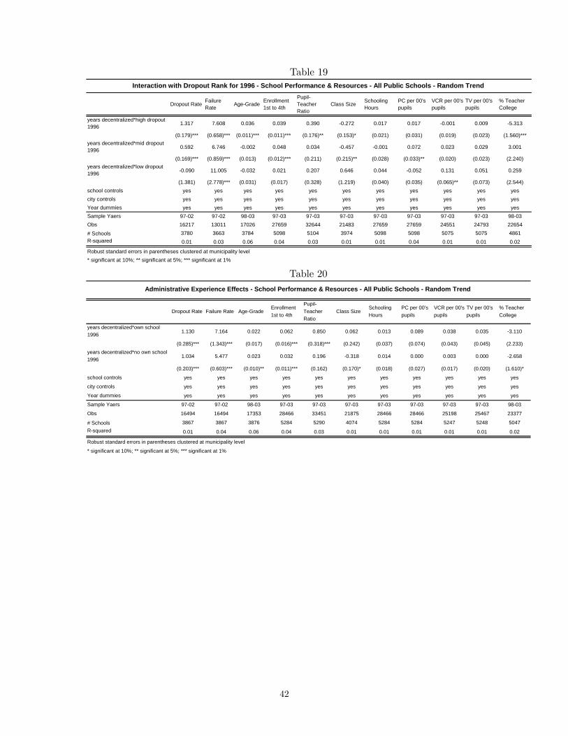
Table 19

Dropout Rate FailureRate Age­Grade Enrollment

1st to 4th

Pupil­TeacherRatio

Class Size SchoolingHours

PC per 00'spupils

VCR per 00'spupils

TV per 00'spupils

% TeacherCollege

years decentralized*high dropout1996 1.317 7.608 0.036 0.039 0.390 ­0.272 0.017 0.017 ­0.001 0.009 ­5.313

(0.179)*** (0.658)*** (0.011)*** (0.011)*** (0.176)** (0.153)* (0.021) (0.031) (0.019) (0.023) (1.560)***years decentralized*mid dropout1996 0.592 6.746 ­0.002 0.048 0.034 ­0.457 ­0.001 0.072 0.023 0.029 3.001

(0.169)*** (0.859)*** (0.013) (0.012)*** (0.211) (0.215)** (0.028) (0.033)** (0.020) (0.023) (2.240)years decentralized*low dropout1996 ­0.090 11.005 ­0.032 0.021 0.207 0.646 0.044 ­0.052 0.131 0.051 0.259

(1.381) (2.778)*** (0.031) (0.017) (0.328) (1.219) (0.040) (0.035) (0.065)** (0.073) (2.544)school controls yes yes yes yes yes yes yes yes yes yes yescity controls yes yes yes yes yes yes yes yes yes yes yesYear dummies yes yes yes yes yes yes yes yes yes yes yesSample Yaers 97­02 97­02 98­03 97­03 97­03 97­03 97­03 97­03 97­03 97­03 98­03Obs 16217 13011 17026 27659 32644 21483 27659 27659 24551 24793 22654# Schools 3780 3663 3784 5098 5104 3974 5098 5098 5075 5075 4861R­squared 0.01 0.03 0.06 0.04 0.03 0.01 0.01 0.04 0.01 0.01 0.02

Robust standard errors in parentheses clustered at municipality level* significant at 10%; ** significant at 5%; *** significant at 1%

Interaction with Dropout Rank for 1996 ­ School Performance & Resources ­ All Public Schools ­ Random Trend

Table 20

Dropout Rate Failure Rate Age­GradeEnrollment1st to 4th

Pupil­TeacherRatio

Class SizeSchoolingHours

PC per 00'spupils

VCR per 00'spupils

TV per 00'spupils

% TeacherCollege

years decentralized*own school1996 1.130 7.164 0.022 0.062 0.850 0.062 0.013 0.089 0.038 0.035 ­3.110

(0.285)*** (1.343)*** (0.017) (0.016)*** (0.318)*** (0.242) (0.037) (0.074) (0.043) (0.045) (2.233)years decentralized*no own school1996 1.034 5.477 0.023 0.032 0.196 ­0.318 0.014 0.000 0.003 0.000 ­2.658

(0.203)*** (0.603)*** (0.010)** (0.011)*** (0.162) (0.170)* (0.018) (0.027) (0.017) (0.020) (1.610)*

school controls yes yes yes yes yes yes yes yes yes yes yes

city controls yes yes yes yes yes yes yes yes yes yes yes

Year dummies yes yes yes yes yes yes yes yes yes yes yes

Sample Yaers 97­02 97­02 98­03 97­03 97­03 97­03 97­03 97­03 97­03 97­03 98­03

Obs 16494 16494 17353 28466 33451 21875 28466 28466 25198 25467 23377

# Schools 3867 3867 3876 5284 5290 4074 5284 5284 5247 5248 5047R­squared 0.01 0.04 0.06 0.04 0.03 0.01 0.01 0.01 0.01 0.01 0.02

Robust standard errors in parentheses clustered at municipality level

* significant at 10%; ** significant at 5%; *** significant at 1%

Administrative Experience Effects ­ School Performance & Resources ­ All Public Schools ­ Random Trend

42

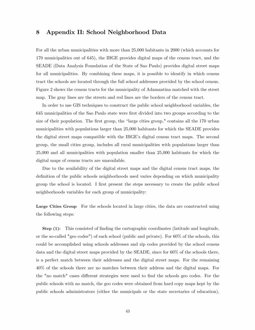
8 Appendix II: School Neighborhood Data

For all the urban municipalities with more than 25,000 habitants in 2000 (which accounts for

170 municipalities out of 645), the IBGE provides digital maps of the census tract, and the

SEADE (Data Analysis Foundation of the State of Sao Paulo) provides digital street maps

for all municipalities. By combining these maps, it is possible to identify in which census

tract the schools are located through the full school addresses provided by the school census.

Figure 2 shows the census tracts for the municipality of Adamantina matched with the street

map. The gray lines are the streets and red lines are the borders of the census tract.

In order to use GIS techniques to construct the public school neighborhood variables, the

645 municipalities of the Sao Paulo state were first divided into two groups according to the

size of their population. The first group, the “large cities group," contains all the 170 urban

municipalities with populations larger than 25,000 habitants for which the SEADE provides

the digital street maps compatible with the IBGE’s digital census tract maps. The second

group, the small cities group, includes all rural municipalities with populations larger than

25,000 and all municipalities with population smaller than 25,000 habitants for which the

digital maps of census tracts are unavailable.

Due to the availability of the digital street maps and the digital census tract maps, the

definition of the public schools neighborhoods used varies depending on which municipality

group the school is located. I first present the steps necessary to create the public school

neighborhoods variables for each group of municipality:

Large Cities Group For the schools located in large cities, the data are constructed using

the following steps:

Step (1): This consisted of finding the cartographic coordinates (latitude and longitude,

or the so-called "geo codes") of each school (public and private). For 60% of the schools, this

could be accomplished using schools addresses and zip codes provided by the school census

data and the digital street maps provided by the SEADE, since for 60% of the schools there,

is a perfect match between their addresses and the digital street maps. For the remaining

40% of the schools there are no matches between their address and the digital maps. For

the "no match" cases different strategies were used to find the schools geo codes. For the

public schools with no match, the geo codes were obtained from hard copy maps kept by the

public schools administrators (either the municipals or the state secretaries of education),

43

that indicates schools location. For the “no match” private schools, the geo codes were

obtained through phone calls and manual searches on hard copy maps.

Step (2): This consisted of defining the public school neighborhoods and then aggregat-

ing the census tract data for the defined neighborhoods. The neighborhood for each public

school was defined as the area where the potential public school pupils are located. Since the

law dictates that public school students must attend the closest school to their homes, the

public schools’neighborhood was defined as the area closest to a public school than to any

other public school (these areas are given by the Voronoi Diagram). Due to public schools at-

trition in the 1996-2003 period and the fact the neighborhood boundaries are sensitive to the

number of schools within the municipality, the public school neighborhoods were redesigned

for every year in the sample. Once the boundaries of the schools’neighborhood were defined,

all the 527 variables of the census tracts within the schools’neighborhood were aggregated

to the neighborhood level.

Step (3): This consisted of interpolating the household variables in the 2000 census with

the 1991 census. The major problem in performing this interpolation relies on the fact that

the 1991 Population Census is not organized in census tracts. However, since both censuses

(2000 and 1991) variables are available at the municipality level, the interpolation at the

municipal level is possible. Under the assumption that the time variation of the variables

aggregated at the municipal level are a good proxy for the time variation of the variables

aggregated at the school neighborhood level, it is thus possible to interpolate the variables at

the school neighborhood level. In short, I use the same line obtained for the interpolation of

variable A (let us say) aggregated at municipal level to interpolate the very same variable A

aggregated at the school neighborhood level. Based on this interpolation procedure I inputted

the household variables aggregated at the school neighborhood level for every public school

for the 8 years of the sample (1996 to 2003).

Small Cities Group As consequence of the unavailability of the census tract digital maps

for the cities in the small cities group, it is not possible to identify the census tract where

the schools are located. It is thus impossible to define the schools’neighborhoods as defined

for the schools located at the large cities group. To overcome this problem, I first classified

the schools located in each municipality into two groups according to the region (urban or

rural) where they are located i.e., rural schools and the urban schools. I then took advantage

of the fact that it is also possible to identify the region (urban or rural) where the census

44

tracts are located to aggregate the household variables (provided by the census tract) for the

rural and urban areas in each municipality. Lastly, the household variables aggregated for

the rural areas were distributed uniformly among the schools located in rural areas, while

the household variables aggregated for the urban areas were distributed uniformly among the

schools located in urban areas. Using the population census data interpolated (between 1991

and 2003) for the rural and urban areas of each municipality, it was then possible to replicate

this procedure for all years the available (1996 to 2003).

References

[1] Araujo, M. C. , Ferreira F.H.G., Lanjouw, P. and Ozler, B. (2006) "Local

inequality and project choice : theory and evidence from Ecuador", World Bank Policy

Research Working Paper No. 3997

[2] Barros, R. P. and Mendonca R. (1998) “The Impact of Three Institutional Inno-

vation in Brazilian Education”in Organization Matters: Agency Problems in Health and

Education in Latin America, Savedoff, W. D, (ed), Inter-American Development Bank,

Washington, DC

[3] Bardhan, P. and Mookherjee, D. (eds) (2005a), Decentralization and Local Gov-

ernments in Developing Countries: A Comparative Perspective, Cambridge, US: MIT

Press

[4] Bardhan, P. and Mookherjee, D. (2005b), “Decentralization, Corruption and Gov-

ernment Accountability: An Overview”in Handbook of Economic Corruption, Elgar, E.

and Rose-Ackerman, S. (eds).

[5] Bertrand, M., Duflo, E. and Mullainathan, S. (2004) “How Much Should We

Trust Differences-in-Differences Estimates?” Quarterly Journal of Economics,119 (1),

249-275

[6] Cameron, A. C. and Tivedi, P. K. (2005), Microeconometrics Methods and App-

plications, Cambridge University Press

[7] Galiani, S., Gertler, P. and Schargrodsky, E. (2005), “School Decentralization:

Helping the Good Get Better but Leaving the Poor Behind”, Working Paper , Buenos

Aires, Universidade de San Andres

45

[8] Heckman and Robb (1995) " "Alternative Methods for Evaluating the Impact of

Interventions", in Logitudinal Analysis of Labor Market Data, Heckman and Singer (eds),

New York: Cambridge University Press, pp. 243-287.

[9] Heckman and Hotz (1989) ‘Choosing Among Alternatives Nonexperimental Methods

for Estimating the Impact of Social Programs: The Case of Manpower Training’, Journal

of American Statistical Association, 84, 862-874.

[10] Jimenez, E. and Sawada Y. (1999), “Do Community-Managed Schools Work? An

Evolution of El Salvador’s EDUCO Program”, The World Bank Economic Review, 13,

(3), 415-441

[11] King, E. and Ozler B. (1998), “What’s Decentralization Got To Do With Learning?

The Case of Nicaragua’s School Autonomy Reform”, The World Bank Working Paper

Series on Impact Evaluation of Education Reforms

[12] Rodriguez, C. (2006) “Households´ schooling behavior and Political Economy Trade-

offs After Decentralization”, Working Paper, Universidad de los Andes, Colombia

[13] Tulchin, J. S. and Selee, A. (eds) (2004) Decentralization and Democratic Gover-

nance in Latin America, WoodrowWilson International Center for Scholars, Washington,

D.C.

[14] Winkler, D. R. and Gershberg A. I. (2000) , “Education Decentralization in Latin

America: The Effects on the Quality of Schooling”LCSHD Paper Series No 59, The

World Bank, Washington, D.C.

[15] Wooldridge, J. M. (2002) Econometric Analysis of Cross Section and Panel Data,

MIT press

46