This article was downloaded by: [University of Sussex Library]On: 25 August 2014, At: 14:45Publisher: Taylor & FrancisInforma Ltd Registered in England and Wales Registered Number: 1072954 Registered office: Mortimer House,37-41 Mortimer Street, London W1T 3JH, UK

International Journal of ControlPublication details, including instructions for authors and subscription information:http://www.tandfonline.com/loi/tcon20

Feedback control and the arrow of timeTryphon T. Georgiou a & Malcolm C. Smith ba Department of Electrical and Computer Engineering , University of Minnesota ,Minneapolis, MN 55455, USAb Department of Engineering , University of Cambridge , Cambridge, CB2 1PZ, UKPublished online: 23 Jun 2010.

To cite this article: Tryphon T. Georgiou & Malcolm C. Smith (2010) Feedback control and the arrow of time, InternationalJournal of Control, 83:7, 1325-1338, DOI: 10.1080/00207171003682655

To link to this article: http://dx.doi.org/10.1080/00207171003682655

PLEASE SCROLL DOWN FOR ARTICLE

Taylor & Francis makes every effort to ensure the accuracy of all the information (the “Content”) containedin the publications on our platform. However, Taylor & Francis, our agents, and our licensors make norepresentations or warranties whatsoever as to the accuracy, completeness, or suitability for any purpose of theContent. Any opinions and views expressed in this publication are the opinions and views of the authors, andare not the views of or endorsed by Taylor & Francis. The accuracy of the Content should not be relied upon andshould be independently verified with primary sources of information. Taylor and Francis shall not be liable forany losses, actions, claims, proceedings, demands, costs, expenses, damages, and other liabilities whatsoeveror howsoever caused arising directly or indirectly in connection with, in relation to or arising out of the use ofthe Content.

This article may be used for research, teaching, and private study purposes. Any substantial or systematicreproduction, redistribution, reselling, loan, sub-licensing, systematic supply, or distribution in anyform to anyone is expressly forbidden. Terms & Conditions of access and use can be found at http://www.tandfonline.com/page/terms-and-conditions

International Journal of ControlVol. 83, No. 7, July 2010, 1325–1338

Feedback control and the arrow of time

Tryphon T. Georgioua and Malcolm C. Smithb*

aDepartment of Electrical and Computer Engineering, University of Minnesota, Minneapolis,MN 55455, USA; bDepartment of Engineering, University of Cambridge, Cambridge, CB2 1PZ, UK

(Received 24 January 2009; final version received 7 February 2010)

The purpose of this article is to highlight the central role that the time asymmetry of stability plays in feedbackcontrol. We show that this provides a new perspective on the use of doubly-infinite or semi-infinite time-axes forsignal spaces in control theory. We then focus on the implication of this time asymmetry in modellinguncertainty, regulation and robust control. We point out that modelling uncertainty and the ease of controldepend critically on the direction of time. We also discuss the relationship of this control-based time-arrow withthe well-known arrows of time in physics.

Keywords: stability; feedback control; thermodynamics; time-asymmetry; robust control; reversibility

1. Introduction

The origin and implications of the ‘arrow of time’ isone of the deepest and least understood subjects ofphysics. The ‘arrow’ is an intrinsic part of the world aswe know it. Yet, its emergence in thermodynamics andcosmology, from physical laws which are apparentlyimpervious to it, remains a controversial subject (Price1996). At first sight, this subject may seem uncon-nected with the theory of feedback control. However,starting from the very basic fact that our notion ofstability in the sense of Lyapunov is time-asymmetric,we argue that the ‘arrow of time’ does have importantimplications on modelling and uncertainty, robustnessof stability, as well as on the topology for the study ofthe dynamics of feedback interconnections.

The circle of ideas that gave rise to this articlebegan in a short note published by Georgiou andSmith (1995). There, it was pointed out that thedoubly-infinite time-axis presents some ‘intrinsic diffi-culties’ for developing a suitable input–output systemstheory – difficulties that are not present in the semi-infinite time-axis setting. These difficulties are notmere mathematical technicalities. Rather, they relatefundamentally to the consistency of the theoryof stabilisability across different frameworks.Subsequently, a number of works were written whichshed light on the problem (Jacob and Partington 2000;Makila 2002, 2003; Makila and Partington 2002, 2004,2006; Jacob 2003, 2004; Partington 2004). This articletakes a fresh look and traces the origin of the ‘puzzle’

to the arrow of Lyapunov stability, and then, explores

the relevance of this arrow to the topology of

dynamical systems and feedback theory.The relationship of the modern theory of dynami-

cal systems with classical physics and thermodynamics

is a developing one. A classical contribution by

Nyquist (1928) and Johnson (1928) is a derivation of

the electromotive force due to thermal agitation in

conductors. Brockett and Willems (1978) treated the

issue of irreversibility from the point of view of

stochastic control theory. More recently, Haddad,

Chellaboina, and Nersesov (2005) have sought to

formalise classical thermodynamics in the mathemat-

ical language of modern dynamical systems (see also

Sandberg, Delvenne, and Doyle 2007a, b). Mitter and

Newton (2005) have studied information flow and

entropy in the context of the Kalman filter. In

Sandberg et al. (2007a, b) it is shown that a linear

macroscopic dissipative system can be approximated

by a linear lossless microscopic system over arbitrary

long-time intervals. Our point of view here is influ-

enced by Price (1996) and is somewhat different to

the above references in that our main goal is to

highlight a time-asymmetry, point out its implications

and discuss its relationship to other well-known

asymmetries.This article begins by providing a new explanation

of the issues raised in Georgiou and Smith (1995) with

regard to an input–output theory for the doubly-

infinite time-axis. In Section 3 we introduce the time-

*Corresponding author. Email: mcs@eng.cam.ac.uk

ISSN 0020–7179 print/ISSN 1366–5820 online

� 2010 Malcolm C. Smith

DOI: 10.1080/00207171003682655

http://www.informaworld.com

Dow

nloa

ded

by [

Uni

vers

ity o

f Su

ssex

Lib

rary

] at

14:

45 2

5 A

ugus

t 201

4

conjugation operator and discuss the implications ofthe time-arrow in optimal control problems.In Section 4 we analyse the effect of the time-arrowon modelling uncertainty; we show that dynamicalsystems which are close in the usual sense, that acommon controller can stabilise and give similarclosed-loop responses for either, may not be closewhen the time-arrow is reversed. Then, in Section 5, wefurther illuminate the inherent time-asymmetry in ourability to control a dynamical system with two specificexamples. These can be thought of as examples of timeirreversible feedback phenomena (Section 5.2). InSection 6 we briefly discuss the arrow of time inphysics and its relation to the time-arrow of feedbackstability. Finally, in Section 7 we consider the feedbackloops with small time delays and discuss the contrast-ing effects of delays and predictors and the connectionwith the arrow of time.

2. Time-asymmetry and stability

2.1 Input–output and Lyapunov stability

We focus on finite-dimensional linear dynamicalsystems which, for the most part, are assumed to betime-invariant. The dimensions of input, state andoutput (column) vectors, as well as the consistent sizesof transformation matrices in state-space models, aresuppressed for notational simplicity. The followingresult is basic and well known (cf. Willems 1970,pp. 52–53; Green and Limebeer 1995, p. 82).

Proposition 2.1: Let P be a linear time-invariantfinite-dimensional system which is controllable andobservable and is specified by

_x ¼ Axþ Bu, ð1Þ

y ¼ CxþDu, ð2Þ

with an initial condition x(0)¼ 0. Then y2L2[0,1) forall u2L2[0,1) if and only if the matrix A is Hurwitz.Moreover, if this condition holds, y is determineduniquely by y(s)¼ (C(sI�A)�1BþD)u(s), where^ denotes the Laplace transform.

Many variants and extensions of the result arefamiliar: signal spaces with different norms can also beused; there is a finite-gain property relating theL2-norms of y and u; even with x(0) 6¼ 0 the mainequivalence in the proposition still holds. Here wewould like to highlight the fact that the resultestablishes an equivalence between stability defined interms of the forced response and stability defined interms of the free response, i.e. an equivalence betweenbounded-input/bounded-output (BIBO) stability andLyapunov stability for a system with non-zero initial

condition operating on the positive time-axis.Asymptotic stability in the sense of Lyapunov isobviously a time-asymmetric concept since conver-gence of the state vector is required as t tends to PLUSinfinity, starting from an arbitrary initial condition att¼ 0. In itself, BIBO stability does not appear to havethis asymmetry. Yet, an asymmetry is brought inthrough the support of the signals being [0,1).

To further illustrate the point we can write downthe following obvious corollary of Proposition 2.1,obtained by running time backwards from 0 to �1.By changing the support of the signal spaces from thepositive half-line to the negative half-line stabilitydefined through the forced response (BIBO stability)becomes equivalent to asymptotic stability in the senseof Lyapunov for the reversed time-direction as t tendsto MINUS infinity.

Proposition 2.2: Let P be a linear system as inProposition 2.1 with x(0)¼ 0. Then y2L2(�1, 0] forall u2L2(�1, 0] if and only if the matrix �A isHurwitz.

We now turn to the situation where inputs andoutputs may have support on the doubly-infinitetime-axis. In this case the following proposition holds(see e.g. Zhou, Doyle, and Glover 1995, p. 101).

Proposition 2.3: Let P be a linear system as inProposition 2.1. Then for all u2L2(�1,1) thereexists y2L2(�1,1) satisfying (1) and (2) if and onlyif A has no imaginary-axis eigenvalues. Moreover, if thiscondition holds, y is determined uniquely by y(s)¼(C(sI�A)�1BþD)u(s).

We remark that Proposition 2.3 is the naturalgeneralisation of Proposition 2.1 when systems areviewed as operators. A linear system in Proposition 2.1becomes a multiplication operator on the Fouriertransformed spaces. The operator is bounded if andonly if the ‘symbol’ (the transfer-function) belongs toH1, which under the controllability and observabilityassumption is equivalent to A being Hurwitz. On thedouble-axis a multiplication operator on the Fouriertransformed spaces is bounded if and only if thesymbol belongs to L1 – which for rational symbolsexcludes only poles on the imaginary axis.

In Proposition 2.3 there is no longer any relation-ship between a notion of BIBO stability and asympto-tic stability in the sense of Lyapunov, in eithertime-direction, for the autonomous system withx(0) 6¼ 0. Clearly, both A and �A may fail to beHurwitz. Since only the existence of some y2L2(�1,1) is required for a given u2L2(�1,1),and the free motion solutions of (1) are ignored, this isnot surprising. Propositions 2.1 and 2.2, by contrast,establish a connection between BIBO stability, for

1326 T.T. Georgiou and M.C. Smith

Dow

nloa

ded

by [

Uni

vers

ity o

f Su

ssex

Lib

rary

] at

14:

45 2

5 A

ugus

t 201

4

signal spaces with support on a half-axis, and

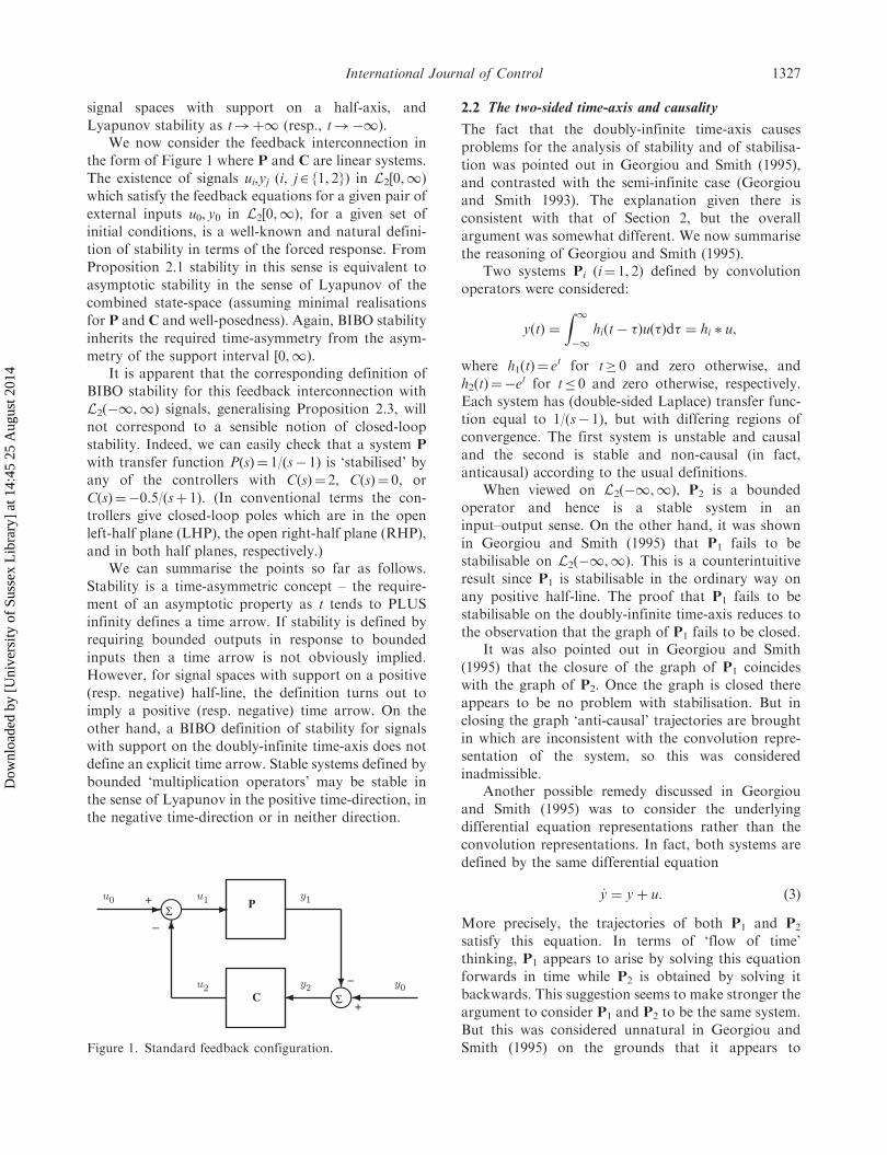
Lyapunov stability as t!þ1 (resp., t!�1).We now consider the feedback interconnection in

the form of Figure 1 where P and C are linear systems.

The existence of signals ui,yj (i, j2 {1, 2}) in L2[0,1)

which satisfy the feedback equations for a given pair of

external inputs u0, y0 in L2[0,1), for a given set of

initial conditions, is a well-known and natural defini-

tion of stability in terms of the forced response. From

Proposition 2.1 stability in this sense is equivalent to

asymptotic stability in the sense of Lyapunov of the

combined state-space (assuming minimal realisations

for P and C and well-posedness). Again, BIBO stability

inherits the required time-asymmetry from the asym-

metry of the support interval [0,1).It is apparent that the corresponding definition of

BIBO stability for this feedback interconnection with

L2(�1,1) signals, generalising Proposition 2.3, will

not correspond to a sensible notion of closed-loop

stability. Indeed, we can easily check that a system P

with transfer function P(s)¼ 1/(s� 1) is ‘stabilised’ by

any of the controllers with C(s)¼ 2, C(s)¼ 0, or

C(s)¼�0.5/(sþ 1). (In conventional terms the con-

trollers give closed-loop poles which are in the open

left-half plane (LHP), the open right-half plane (RHP),

and in both half planes, respectively.)We can summarise the points so far as follows.

Stability is a time-asymmetric concept – the require-

ment of an asymptotic property as t tends to PLUS

infinity defines a time arrow. If stability is defined by

requiring bounded outputs in response to bounded

inputs then a time arrow is not obviously implied.

However, for signal spaces with support on a positive

(resp. negative) half-line, the definition turns out to

imply a positive (resp. negative) time arrow. On the

other hand, a BIBO definition of stability for signals

with support on the doubly-infinite time-axis does not

define an explicit time arrow. Stable systems defined by

bounded ‘multiplication operators’ may be stable in

the sense of Lyapunov in the positive time-direction, in

the negative time-direction or in neither direction.

2.2 The two-sided time-axis and causality

The fact that the doubly-infinite time-axis causes

problems for the analysis of stability and of stabilisa-

tion was pointed out in Georgiou and Smith (1995),

and contrasted with the semi-infinite case (Georgiou

and Smith 1993). The explanation given there is

consistent with that of Section 2, but the overall

argument was somewhat different. We now summarise

the reasoning of Georgiou and Smith (1995).Two systems Pi (i¼ 1, 2) defined by convolution

operators were considered:

yðtÞ ¼

Z 1�1

hiðt� �Þuð�Þd� ¼ hi � u,

where h1(t)¼ et for t� 0 and zero otherwise, and

h2(t)¼�et for t� 0 and zero otherwise, respectively.

Each system has (double-sided Laplace) transfer func-

tion equal to 1/(s� 1), but with differing regions of

convergence. The first system is unstable and causal

and the second is stable and non-causal (in fact,

anticausal) according to the usual definitions.When viewed on L2(�1,1), P2 is a bounded

operator and hence is a stable system in an

input–output sense. On the other hand, it was shown

in Georgiou and Smith (1995) that P1 fails to be

stabilisable on L2(�1,1). This is a counterintuitive

result since P1 is stabilisable in the ordinary way on

any positive half-line. The proof that P1 fails to be

stabilisable on the doubly-infinite time-axis reduces to

the observation that the graph of P1 fails to be closed.It was also pointed out in Georgiou and Smith

(1995) that the closure of the graph of P1 coincides

with the graph of P2. Once the graph is closed there

appears to be no problem with stabilisation. But in

closing the graph ‘anti-causal’ trajectories are brought

in which are inconsistent with the convolution repre-

sentation of the system, so this was considered

inadmissible.Another possible remedy discussed in Georgiou

and Smith (1995) was to consider the underlying

differential equation representations rather than the

convolution representations. In fact, both systems are

defined by the same differential equation

_y ¼ yþ u: ð3Þ

More precisely, the trajectories of both P1 and P2

satisfy this equation. In terms of ‘flow of time’

thinking, P1 appears to arise by solving this equation

forwards in time while P2 is obtained by solving it

backwards. This suggestion seems to make stronger the

argument to consider P1 and P2 to be the same system.

But this was considered unnatural in Georgiou and

Smith (1995) on the grounds that it appears to

u0 u1 y1

u2 y2 y0

+S P

−

–

C S+

Figure 1. Standard feedback configuration.

International Journal of Control 1327

Dow

nloa

ded

by [

Uni

vers

ity o

f Su

ssex

Lib

rary

] at

14:

45 2

5 A

ugus

t 201

4

abandon any notion of causality, or that it leaves thedirection of time undefined.

The discussion of Section 2 allows the difficultiespointed out in Georgiou and Smith (1995) to beexplained in a new way. Let us suppose we are willingto accept the closure of the graph of P1 which makes it‘stabilisable’ on the double-axis in a BIBO sense. Asexplained, P1 and P2 can now be thought of as one andthe same system defined by (3) – a state-spacedescription as in (1) and (2) solved forwards orbackwards as desired. Does the closure of the graphresolve the difficulty pointed out in Georgiou andSmith (1995)? The answer is no, since the notion ofstability does not correspond to the usual notions. Asis made clear by Proposition 2.3, the feedback systemmay turn out to be stable in a conventional sense in theforward, backward or neither time-directions.

2.3 The work of Makila, Partington and Jacob et al.

A number of interesting observations and contribu-tions have followed from Georgiou and Smith (1995)which we would like to comment on here. The fact thata causal system on the double-axis can have a non-causal closure has led to a study of ‘closability’ and‘causal closability’ as questions in their own right.Makila (2002) has shown that the lack of causalclosability for the example of Georgiou and Smith(1995) extends to general Lp spaces on the double-axis.Jacob and Partington (2000) gave general characterisa-tions of the graphs of time-invariant systems andderived necessary and sufficient conditions for theclosure of a closable system to be causal. Makila andPartington (2006) considered weighted L2-spaces onthe double-axis and showed that, when signals havevery rapid decrease to zero towards �1, causalconvolution operators may be closed operators. (Sothere is no issue of causality being lost due to theoperation of closure.)

On the question of stabilisation on the doubletime-axis, Jacob (2004) has made an interestingsuggestion. We have seen already that closing thegraph and applying the BIBO stability definition failsto recover the usual concept of stability. Jacobproposed that causality of the closed-loop operatorsof the feedback system be added as an extra require-ment. Jacob showed that the resulting characterisationof stability agrees with the usual definitions for lineartime-invariant systems. In the context of this article wecan re-interpret this result by saying that the causalitycondition forces the positive time-arrow into feedbacksystem stability. We can understand this as follows. InJacob and Partington (2000) it is shown that a closedlinear time-invariant system is causal on L2(�1,1) if

and only if the corresponding transfer function belongsto a certain Smirnov class. For finite-dimensionalsystems this is equivalent to the transfer functionhaving no right half-plane poles. Thus, inProposition 2.3, if P is required to be causal, BIBOstability agrees with Lyapunov stability with thepositive time-arrow.

Makila and Partington (2006) make an interestingobservation on the possible extension of Jacob’s ideato the time-varying situation. They consider a causal,convolution operator derived from the underlyingdifferential equation

_yðtÞ þ aðtÞ yðtÞ ¼ uðtÞ, ð4Þ

where a(t)¼�1 for t� 0 and a(t)¼þ1 for t4 0 andpoint out that the closure of the L2(�1, 1) graph ofthe convolution system is not the graph of an operator.Essentially this boils down to the fact that there arefree motion solutions y(t)¼ ce�jtj, u(t)¼ 0, where c is aconstant, which can be approximated arbitrarilyclosely by elements of the graph. This raises thequestion of whether the approach of Jacob can recovera theory of stabilisation which is consistent with thesingle-axis case. At the same time, it is pointed out thatthe system is stabilisable in a Lyapunov sense by thefeedback

uðtÞ ¼ �2yðtÞ: ð5Þ

In the present context this example highlights the carethat is needed in defining stability for time-varyingsystems, even in the conventional sense. The open-loopsystem (4) is Lyapunov stable in the forward time-direction for any initial condition specified at any time(either positive or negative), but not uniformly so.Incidentally, the same is true for stability in thebackwards time-direction. With the feedback (5) inforce the system becomes uniformly stable in the senseof Lyapunov in the forward time-direction and unsta-ble in reverse. In the perspective of this article, anymethod to force agreement between BIBO stability onthe double-axis and conventional notions (such asrequiring causality of the closed loop operators) mightbe seen as tantamount to directly imposing the desiredtime arrow within the stability definition.

Makila and Partington (2002, 2004, 2006) haveadvocated the use of a two-operator model for systems

on the doubly infinite time-axis in the form Ay¼Bu,

where A, B are causal, bounded operators, in contrast

to a single-operator model y¼Pu, where P is causal

and possibly unbounded. Closed-loop stability is

defined as the existence of a causal, bounded inverse

of the feedback system operator mapping system

inputs to exogenous disturbances. Since this definition

incorporates a causality requirement on the closed-loop

1328 T.T. Georgiou and M.C. Smith

Dow

nloa

ded

by [

Uni

vers

ity o

f Su

ssex

Lib

rary

] at

14:

45 2

5 A

ugus

t 201

4

system, there is evidently a close relationship between

this idea and the approach of Jacob.Bian, French, and Pillai (2008) consider the puzzle

raised in Georgiou and Smith (1995) from a beha-vioural point of view. As is customary in the

behavioural theory, Bian et al. (2008) define thesystem behaviour to include all admissible autonomous

as well as forced responses on the doubly-infinite time-axis. In contrast, stability requires boundedness of

signals when restricted to a positive half-line. Theauthors recognise that the behavioural approach is

‘perhaps halfway between a double and a half line’approach. Indeed, their conclusion is consistent with

the viewpoint in the current article that a timeasymmetry needs to be imposed on any double-axis

theory for a proper treatment of stability and

stabilisation.

3. Time-asymmetry and optimal regulation

This section focuses on the time-asymmetry of the

definition of stability and its implications in the contextof optimal regulation. Firstly, a time-conjugation

operator will be defined as well as the concepts off-stability and b-stability. Then the finite-horizon

quadratic regulator problem will be considered for a

system running forwards in time and backwards intime, and it will be shown that the optimal cost is

generally different. The infinite-horizon (asymptotic)regulator will also be considered in the same way. It

will be shown that the optimal cost can be expressed interms of the two extremal solutions of the appropriate

algebraic Riccati equation. The result shows that easeof optimal regulation depends on the time-direction.

3.1 The time-conjugation operator, f-stability andb-stability

Let P denote a dynamical system described by the

state-space equations in (1) and (2), initialised at timezero and running forwards in time. Let J denote the

operation on P which corresponds to solving (1) and(2) backwards from t¼ 0 followed by a flip of the time-

axis (so the new system runs forward again). Morespecifically we set t1¼�t, so that

d

dt¼ �

d

dt1,

and then replace t1 by t which results in

� _x ¼ Axþ Bu, with xð0Þ ¼ x0

y ¼ CxþDu

for the system JðPÞ. The effect on the transfer functionis as follows: if P has transfer function P(s), then JðPÞ

has transfer function P(�s).Define the system P to be f-stable if A is Hurwitz,

and define P to be b-stable if JðPÞ is f-stable, orequivalently, if �A is Hurwitz. It is immediatelyobvious that a linear time-invariant system of thetype (1) and (2) can never be both f-stable and b-stable.Similarly, a controller cannot make the closed-loopsystem both f-stable and b-stable at the same time.

3.2 The finite-horizon linear quadratic regulator

Let P be a linear time-invariant system which iscontrollable and observable and described by (1) and(2), as before, with D¼ 0 and x(0)¼x0. Considerthe problem of the regulation of P with criterion

J ¼

Z T

0

ð yðtÞ0QyðtÞ þ uðtÞ0RuðtÞÞdtþ xðT Þ0HxðT Þ:

This has solution

uðtÞ ¼ �R�1B0SðtÞxðtÞ, ð6Þ

where

� _SðtÞ ¼ SðtÞAþ A0SðtÞ � SðtÞBR�1B0SðtÞ þ C0QC

ð7Þ

and S(T )¼H, with optimal cost Jf,T ¼ x00Sð0Þx0(Anderson and Moore 1990). When P runs backwardsin time from x(0)¼ x0 with cost

J ¼

Z 0

�T

ð yðtÞ0QyðtÞ þ uðtÞ0RuðtÞÞdtþ xð�T Þ0Hxð�T Þ,

we can check that the optimal control is still given by(6) where S(t) satisfies (7) with S(�T )¼�H, and thatthe optimal cost is Jb,T ¼ �x

00Sð0Þx0. It can be readily

verified that S(0) for the forward case is, in general,different from �S(0) for S(t) found for the backwardcase, and so the optimal cost is different in the twocases, e.g. if A¼B¼C¼Q¼R¼T¼ 1 and H¼ 10,then S(0)¼ 2.5415 in the forward case and �S(0)¼0.5495 in the backward case.

3.3 The infinite-horizon linear-quadratic regulator

Again let P be a linear time-invariant system which iscontrollable and observable and described by (1)and (2) with D¼ 0 and x(0)¼ x0. It is well known(Anderson and Moore 1990) that

J ¼

Z 10

ð yðtÞ0QyðtÞ þ uðtÞ0RuðtÞÞdt ð8Þ

International Journal of Control 1329

Dow

nloa

ded

by [

Uni

vers

ity o

f Su

ssex

Lib

rary

] at

14:

45 2

5 A

ugus

t 201

4

has a minimum given by Jf,1 ¼ x00Sþx0 where Sþ is theunique positive-definite solution to the algebraicRiccati equation

A0Sþ SA� SBR�1B0Sþ C0QC ¼ 0: ð9Þ

It is also well known that Sþ is the unique solution of(9) for which A�BR�1B0S has all its eigenvalues in theopen LHP. In the terminology of the present article wecan say that Sþ is the unique solution of (9) whichmakes the system (1) and (2) f-stable with the control-ler u¼�R�1B0Sx.

What happens if we require the minimisation of

J ¼

Z 0

�1

ð yðtÞ0QyðtÞ þ uðtÞ0RuðtÞÞdt ð10Þ

for (1)–(2) running backwards in time? This is the sameas the conventional problem for the system JðPÞ. It iseasy to see that the minimum is given by Jb,1 ¼�x00S�x0 where S� is the unique negative-definitesolution to (9). It is also well known that S� is theunique solution of (9) for which A�BR�1B0S has allits eigenvalues in the open RHP (Zhou et al. 1995). Inthe terminology of the present article, we can say thatS� is the unique solution of (9) which makes the system(1)–(2) b-stable with the controller u¼�R�1B 0Sx.

In general, Jf,1 ¼ x00Sþx0 and Jb,1 ¼ �x00S�x0 are

different. This shows that ‘difficulty of control’ istime-asymmetric for the standard linear-quadraticregulator on the infinite horizon. The difference canbe significant, e.g. if A¼ 1, B¼ �, C¼ 1, Q¼ 1 andR¼ 1 then Sþ¼ 2/�2þ 1/2þO(�2) and S�¼�1/2þO(�2) for � small.

4. Time-asymmetry and modelling uncertainty

In this section we look at the topology for uncertaintyin feedback control and how this is affected by the timearrow. We will see that dynamical systems which areclose in the usual sense, that a common controller canstabilise them and give a similar closed-loop behaviour,may not be close if time is reversed.

4.1 The gap metric and robustness of stability

Zames and El-Sakkary (1980) introduced a metric ondynamical systems for the purpose of assessingrobustness. This was based on the gap metric used infunctional analysis to study the invertibility ofoperators (Kreın and Krasnosel’skii 1947; Nagy1947). Specifically, systems are considered to beoperators on L2[0,1) with a graph which is a closedsubspace of L2[0,1). Consider two linear systems Pi

(i¼ 1, 2) with transfer functions

PiðsÞ ¼ niðsÞ miðsÞð Þ�1,

where ni(s) and mi(s) are coprime polynomials or, more

generally, right-coprime polynomial matrices. Let

nið�sÞð ÞTniðsÞ þ mið�sÞð Þ

TmiðsÞ ¼ dið�sÞð ÞTdiðsÞ

with det(di(s)) a Hurwitz polynomial and ( )T repre-

senting the matrix transpose – the existence of such a

polynomial (matrix) di(s) is a standard result in the

theory of canonical factorisation (Youla 1961). Then,

GPi,H2:¼

miðsÞðdiðsÞÞ�1

niðsÞðdiðsÞÞ�1

!H2 :¼ GiðsÞH 2

is (the Fourier transform of) the graph of Pi, for

i¼ 1, 2, where H2 is the Hardy subspace of L2( jR) with

functions having analytic continuation in the RHP.

Thus, the graph symbol Gi(s) generates the graph of Pi

as its range. Then the gap between P1 and P2 is defined

to be

�H2ðP1,P2Þ :¼ k�GP1,H2 ��GP2,H2 k

where �K denotes orthogonal projection onto a closed

subspace K.Let the feedback configuration of Figure 1 be

denoted by [P,C], where P and C are linear systems

defined as operators on L2[0,1), which may possibly

be unbounded. Define

HP,C :¼I

P

� �ðI� PCÞ�1ðI �CÞ

to be the operator mapping uT0 yT0

� �Tto uT1 y

T1

� �T. The

following are basic robustness results for gap metric

uncertainty.

Proposition 4.1 (Georgiou and Smith 1990): Assume

that the closed-loop system [P,C] is f-stable. Then,

[P1,C] is f-stable for all P1 such that �H2(P,P1)� b if

and only if b5 bP,C where

bP,C :¼ kHP,Ck�11 :

Proposition 4.2 (Zames and El-Sakkary 1980):

Assume that the closed-loop system [P,C] is f-stable.

Then, the following are equivalent:

(i) �H2(Pn, P)! 0 as n!1.

(ii) HPn,Cis f-stable for sufficiently large n and

kHPn,C�HP,Ck1! 0 as n!1.

Proposition 4.2 was the primary justification for

the claim in Zames and El-Sakkary (1980) that the gap

metric defines the ‘correct’ topology for the robustness

of feedback systems. In the present context, it can be

seen that the choice of a signal space with support on

the positive half-line is essential in achieving an

appropriate topology. To emphasise the point, if

L2[0,1) were replaced by L2(�1, 0] then the above

1330 T.T. Georgiou and M.C. Smith

Dow

nloa

ded

by [

Uni

vers

ity o

f Su

ssex

Lib

rary

] at

14:

45 2

5 A

ugus

t 201

4

proposition would hold with f-stability replaced by

b-stability.Let us consider the case where systems are defined

on L2(�1,1). Then we define

�L2ðP1,P2Þ :¼ k�GP1,L2 ��GP2,L2 k,

where

G Pi,L2 :¼ GiðsÞL2

and L2 :¼L2(�j1, j1). With this definition, GP,L2is

always closed, but may contain ‘non-causal’ input–

output pairs as pointed out in Georgiou and Smith

(1995) (see also Section 2.2). It is easy to construct

examples to demonstrate that the convergence of

�L2(Pn,P) to zero does not allow any closed-loop

stability prediction, e.g. [P,C] f-stable does not imply

[Pn,C] f-stable for sufficiently large n.Vinnicombe (1993) introduced a new metric �v(�, �)

on dynamical systems which defines the same topology

as �H2(�, �), and which satisfies the following inequality:

�L2 ð�, �Þ � �vð�, �Þ � �H2ð�, �Þ:

The v-gap between P1 and P2 is defined as follows:

�vðP1,P2Þ :¼

�L2 ðP1,P2Þ if

wnoðdetðG2ð�sÞTG1ðsÞÞÞ ¼ 0,

1 otherwise,

8><>:

ð11Þ

where wno(g(s)) denotes the winding number about the

origin of g(s), as s traces the standard Nyquist

D-contour (Vinnicombe 1993, 2001). A simple expres-

sion for �L2(�, �) can be obtained using left fractional

representations – let PiðsÞ ¼ ð ~miðsÞÞ�1 ~niðsÞ be a left-

coprime polynomial fraction, ~di the Hurwitz polyno-

mial matrices which satisfy

~niðsÞ ~nið�sÞð ÞTþ ~miðsÞ ~mið�sÞð Þ

T¼ ~diðsÞð ~dið�sÞÞ

T,

and define

~GiðsÞ :¼ �ð ~diðsÞÞ�1 ~niðsÞ, ð ~diðsÞÞ

�1 ~miðsÞ� �

for i¼ 1, 2. The graph of Pi is the kernel of multipli-

cation by ~GiðsÞ (in the respective space of signals H2 or

L2). The L2-gap can now be expressed as

�L2ðP1,P2Þ :¼ k ~G2ðsÞG1ðsÞk1:

It turns out that Propositions 4.1 and 4.2 both hold

with �H2replaced by �v (Vinnicombe 1993). Since

�L2¼ �v, when

wnoðdetðG2ð�sÞTG1ðsÞÞÞ ¼ 0 ð12Þ

holds, this condition effectively imposes a positive time-arrow on the double-axis graph which forces f-stabilityto be retained under small perturbations in �v(�, �). Thisis illustrated by the following result, which can bereadily derived from Vinnicombe (1993, Theorem 4.2)(see also Georgiou, Shankwitz, and Smith 1992).

Proposition 4.3: Let [P,C] be f-stable andsuppose �L2

(Pn,P)! 0 as n!1. Then [Pn,C] isf-stable for all sufficiently large n if and only ifwno(det(Gn(�s)

TG(s)))¼ 0 for all sufficiently large n.

4.2 The effect of the time-arrow on gap distances

We define a forward and a backward v-gap as follows:

�v, f ðP1,P2Þ :¼ �vðP1,P2Þ

�v,bðP1,P2Þ :¼ �vðJðP1Þ,JðP2ÞÞ:

It is straightforward to see that

�L2 ðP1,P2Þ ¼ �L2 ðJðP1Þ,JðP2ÞÞ,

so any difference between �v, f (P1,P2) and �v,b(P1,P2)lies in the winding number condition in (11). Let usexamine this more closely. Note that

detðG2ð�sÞTG1ðsÞÞ ¼

hðsÞ

detðd2ð�sÞÞdetðd1ðsÞÞ,

where

hðsÞ :¼ detðm2ð�sÞTm1ðsÞ þ n2ð�sÞ

Tn1ðsÞÞ: ð13Þ

If �L2(P1,P2)5 1, then it can be shown that

wno(det(G2(�s)TG1(s))) is well defined (Vinnicombe

1993), in which case h(s) admits a canonicalfactorisation

hðsÞ ¼ hþðsÞh�ðsÞ, ð14Þ

where hþ(s) and h�(�s) are Hurwitz polynomials.Thus, wno(det(G2(�s)

TG1(s)))¼ 0 if and only if

degðhþðsÞÞ ¼ degðdetðd1ðsÞÞÞ,

or equivalently

degðh�ðsÞÞ ¼ degðdetðd2ðsÞÞÞ:

It can be shown that the degree of detðdiðsÞÞ is equal tothe McMillan degree of Pi, e.g. using the uniqueness ofnormalised coprime factors over H1 up to a constantunitary transformation and the corresponding state-space realisations (Meyer and Franklin 1987,Vidyasagar 1988; Zhou et al. 1995). Determining thegraph symbol for JðPiÞ requires a canonicalfactorisation

niðsÞð ÞTnið�sÞ þ miðsÞð Þ

Tmið�sÞ ¼ ðdið�sÞÞTdiðsÞ

International Journal of Control 1331

Dow

nloa

ded

by [

Uni

vers

ity o

f Su

ssex

Lib

rary

] at

14:

45 2

5 A

ugus

t 201

4

with detðdiðsÞÞ a Hurwitz polynomial. Again it can be

shown that the degree of detðdiðsÞÞ is equal to the

McMillan degree of Pi. The corresponding wind-

ing number condition in �v,b(P1,P2) can now be

expressed as

wnoðdetððd2ð�sÞ�1Þhð�sÞðd1ðsÞ

�1ÞÞÞ ¼ 0,

which is equivalent to deg(h�(s)) being equal to the

McMillan degree of P1. We therefore obtain the

following result.

Proposition 4.4: Let Pi(s) (i¼ 1, 2) be the ratio-

nal transfer functions of linear time-invariant dynamical

systems as above, with McMillan degrees �i, and

with h, hþ, h� as in (13) and 14). Assume that

�L2(P1,P2)5 1.

(i) The following are equivalent:

(a) �v,f (P1, P2)5 1,(b) deg(hþ(s))¼�1,(c) deg(h�(s))¼�2.

(ii) The following are equivalent:

(a) �v,b(P1,P2)5 1,(b) deg(h�(s))¼�1,(c) deg(hþ(s))¼�2.

(iii) The following are equivalent:

(a) �v, f (P1,P2)¼ �v,b(P1,P2)5 1,(b) �1¼�2¼deg(hþ(s))¼ deg(h�(s)).

In the above proposition, (i) expresses the zero

winding number condition in (11) in an equivalent

form, while (ii) does the same for �v,b(P1,P2). It is

interesting that when the two conditions are combined

as in (iii) the result is a very stringent requirement

which includes the necessity that P1(s) and P2(s) have

the same McMillan degree. This serves to highlight the

fact that ‘unmodelled dynamics’ which may account

for a small error in �v,f (and which may be neglected in

the design of a robust controller) will inevitably

account for a substantial error in �v,b. Perhaps, this

can be best summarised by the observation that, if any

dynamical effects are omitted, the same nominal model

cannot suffice for robust control design in both time-

directions.

Example 4.5: Consider two systems with different

McMillan degrees, e.g. P1(s)¼ 1, P2(s)¼ 1/s. It can be

computed that �v, f ðP1,P2Þ ¼ 1=ffiffiffi2p

. Proposition 4.4

then tells us immediately that �v,b(P1,P2)¼ 1, or

equivalently �v,f (P1,P3)¼ 1 where P3(s)¼�1/s.

Similarly, if P4(s)¼ 1/s2, then Proposition 4.4 tells

us that both �v, f (P1,P4)¼ �v,b(P1,P4)¼ 1 since

P4(s)¼P4(�s).

5. Time-asymmetry and robust control

This section addresses the implications of the time-

asymmetry in the theory of robust control. In partic-

ular, we will also see that a system which is ‘easy’ to

control in one direction of time may be far from easy to

control in the opposite direction.

5.1 Optimal robustness and difficulty of control

In Glover and McFarlane (1989) it was shown that

bP,C could be maximised over all stabilising C and that

this amounts to solving a Nehari problem (Zhou et al.

1995). This optimum value, which we denote by

bopt, f ðPÞ,

can be interpreted as a measure of ease/difficulty of

control, where a value near to 1 means the plant is

‘easy to control’ and a value near 0 means the plant is

‘hard to control’.With the understanding that bopt,f (P) has the

meaning of ‘ease of control’ with respect to the

forward time-arrow for stability, it is interesting to

define

bopt, bðPÞ :¼ bopt, f ðJðPÞÞ,

which represents ‘ease of control’ with respect to the

backwards time-arrow. Our main purpose in defining

bopt,b(P) is to highlight the influence of the time-arrow

in feedback regulation.Let P be a controllable and observable system

which is described by the state-space equations in (1)

and (2), as before. Then, following Glover and

McFarlane (1989) and Georgiou and Smith (1990),

we have

bopt, f ðPÞ ¼ffiffiffiffiffiffiffiffiffiffiffiffiffiffiffiffiffiffiffiffiffiffiffiffiffiffiffiffiffiffiffiffiffi1� �maxðYþXþÞ

p,

where Yþ is the positive definite solution of the Riccati

equation

A0Yþ YA�0 � YCR�1C�Yþ BðI�D�R�1D�ÞB� ¼ 0,

ð15Þ

where A0¼A�BD*R�1C and R¼ IþDD*, and Xþ is

the corresponding solution to the (Y-dependent)

Lyapunov equation

ðA0�YC�R�1CÞ�XþXðA0�YC�R�1C ÞþC�R�1C¼ 0

ð16Þ

for Y¼Yþ. Similarly, it can be seen that

bopt,bðPÞ ¼ffiffiffiffiffiffiffiffiffiffiffiffiffiffiffiffiffiffiffiffiffiffiffiffiffiffiffiffiffiffiffiffiffi1� �maxðY�X�Þ

pð17Þ

1332 T.T. Georgiou and M.C. Smith

Dow

nloa

ded

by [

Uni

vers

ity o

f Su

ssex

Lib

rary

] at

14:

45 2

5 A

ugus

t 201

4

where Y� is the negative definite solution of the Riccati

equation (15) while X� is the corresponding solution to

(16) for Y¼Y�.In the following two examples we will see the

situations where bopt,f(�) and bopt,b(�) are very different.

Example 5.1: Near pole-zero cancellations.

Consider PðsÞ ¼ 1þ �sþ1. Letting �A¼C¼D¼ 1

and B¼ � in Equations (15)–(17) gives

bopt, f ðPÞ ¼

ffiffiffiffiffiffiffiffiffiffiffiffiffiffiffiffiffiffiffiffiffiffiffiffiffiffiffiffiffiffiffiffiffiffiffiffiffiffiffiffiffiffiffiffiffiffiffiffiffiffiffiffiffiffiffiffiffiffi1�

ffiffiffiffiffiffiffiffiffiffiffiffiffiffiffiffiffiffiffiffiffiffiffiffiffi1þ �þ �2=2

p� 1� �=2

2ffiffiffiffiffiffiffiffiffiffiffiffiffiffiffiffiffiffiffiffiffiffiffiffiffi1þ �þ �2=2

pvuut :

It follows that for small values of �,

bopt, f ðP Þ ¼ 1�1

32�2 þOð�3Þ

and hence, bopt,f (P)! 1 as �! 0. On the other hand,

bopt, bðP Þ ¼

ffiffiffiffiffiffiffiffiffiffiffiffiffiffiffiffiffiffiffiffiffiffiffiffiffiffiffiffiffiffiffiffiffiffiffiffiffiffiffiffiffiffiffiffiffiffiffiffiffiffiffiffiffiffiffiffiffiffi1�

ffiffiffiffiffiffiffiffiffiffiffiffiffiffiffiffiffiffiffiffiffiffiffiffiffi1þ �þ �2=2

pþ 1þ �=2

2ffiffiffiffiffiffiffiffiffiffiffiffiffiffiffiffiffiffiffiffiffiffiffiffiffi1þ �þ �2=2

pvuut ,

which leads to

bopt, bðP Þ ¼1

4j�j þOð�2Þ

for small values of �, and hence bopt,b(P)! 0 as �! 0.

This is accounted for by the fact that P(s) has a near

pole-zero cancellation in the LHP, which is innocuous

for f-stabilisation, but highly challenging for

b-stabilisation. The latter is equivalent to f-stabilisation

of P(�s), which has a troublesome near pole-zero

cancellation in the RHP.

Example 5.2: Riding bicycles.

A feedback stability problem in everyday experi-

ence is bicycle riding. An elementary model to study

rider–bicycle stability is given in Astrom, Klein, and

Lennartsson (2005), which gives the following transfer

function from steering angle input to tilt angle:

�Vsþ �V

s2 � , ð18Þ

where �, �, are positive constants and V is the

forward speed. This model does not contain dissipation

effects from either the tyres or the suspension. The

model has one RHP pole, but the zero is in the LHP.

As such, this plant is not too difficult to control.Let us consider what happens if we try to ride the

bicycle backwards in time. This corresponds to trying to

stabilise the plant P(�s) forwards in time. The model

still has one RHP pole, but the zero is also in the RHP,

which makes stabilisation much more difficult. Indeed,

if V� ¼ffiffiffip

, the plant is technically not stabilisable.

It is interesting to note that an experimental bicyclewith the steered wheel at the rear instead of the fronthas a transfer function from steering angle input to tiltangle given by Astrom et al. (2005) (see also Limebeerand Sharp 2006),

�V�sþ �V

s2 � : ð19Þ

This is exactly the transfer function for the conven-tional bicycle ridden backwards in time.

Figure 2 shows the value of bopt,f and bopt,b versus Vwith parameter values �¼ 1/3, �¼ 2 and ¼ 9 (whichare deemed reasonably realistic). Recall that bopt,b isthe same as bopt, f for the rear-wheel steered bicyclemodel (19) at the same V. It can be observed that bopt,bis less than bopt, f for any V. Also, bopt,b is very small forlow V, indicating the difficulty of control, and zero atV¼ 1.5m/s. For larger V, bopt,b increases, indicatingthat control becomes easier. These results are equiva-lent to the rear-wheeled steered bicycle being moredifficult to ride than the front-wheel steered one, butstill being reasonably controllable at higher speeds(Astrom et al. 2005).

5.2 Time irreversible feedback phenomena

The concept of ease or difficulty of control gives athought-provoking perspective on reversibility.Systems which in a limiting situation are very difficultto control (in the sense that bopt,f (P) tends to zero) areunlikely to be observed in nature or technology.Nevertheless, such a system may be easy to control inthe time-reversed direction (Examples 5.1 and 5.2).This is independent of the fact that the underlyingdifferential equation can be integrated equally well in

0 2 4 6 8 10 12 14 16 18 200

0.05

0.1

0.15

0.2

0.25

0.3

0.35

0.4

0.45

0.5

bopt,f vs. Vbopt,bvs. V

V (m/s)

b opt

Figure 2. bopt,f and bopt,b versus V for the bicycle model of(18) with �¼ 1/3, �¼ 2, and ¼ 9.

International Journal of Control 1333

Dow

nloa

ded

by [

Uni

vers

ity o

f Su

ssex

Lib

rary

] at

14:

45 2

5 A

ugus

t 201

4

either time-direction. This is the reminiscent ofphenomena (such as a bottle falling from the tableand shattering into many pieces) that appear to beassociated with an intrinsic direction of time eventhough classical physics would also allow the reversedmotion as a solution (see Section 6 for a furtherdiscussion).

We expand this point in the context of Example 5.2.The loss of stabilisability of the rear-wheeled steeredbicycle at V ¼

ffiffiffip

=� has the following interestingconsequence. Imagine a video of a rear-wheeled steeredbicycle being ridden stably at this critical speed. Let usassume that it is possible to verify from the video theactual speed (e.g. by knowing the frame-rate andobserving markings on the ground). An observer witha good grounding in control theory would be led to theinescapable conclusion that the video had been madewhen the said bicycle was actually being riddenbackwards in space (i.e. with a negative V) and thenplayed backwards in time as well, giving the impressionof a forward motion.

6. The arrow of time in physics

The subject of the ‘arrow of time’ is a well-knownconundrum in physics. The second law of thermody-namics states that the entropy of a system increaseswith time. It is the time-asymmetry in this law whichgives rise to the notion of the ‘thermodynamic arrow oftime’. The classical derivation of the second law instatistical mechanics due to Boltzmann is connectedwith a famous puzzle known as Loschmidt’s paradox(Price 1996). This essentially points out that the laws ofmechanics used in the derivation of the second law aretime-symmetric whereas the conclusion is not.Evidently, the time-asymmetry creeps in through thestatistical assumptions. An illuminating discussion ofthis issue is given in Price (1996). Other arrows of timehave also been defined, for example (i) the ‘psycho-logical arrow’ – the direction in which time passes asperceived by a sentient being (Hawking 1988;Schulman 1997), (ii) the ‘cosmological arrow’ – thedirection of time in which the universe is expanding.Hawking (1988) argues that the thermodynamic andpsychological arrows are always aligned with eachother but these need not always be aligned with thecosmological arrow (though they are at present).

In this article we have described the time-asymmetry in the definition of control systems stabilityas a time-arrow. In the theory of dynamical systemsthere is also the notion of passivity, which againdefines a time-arrow. For electrical circuits the time-arrow of passivity can be seen in the behaviour of theresistor, in contrast to the inductor and capacitor

which are time-symmetric in their operation. If theelectrical resistor were to operate backwards in time,one would observe a resistor gathering low-grade heatfrom the environment and charging up a battery. Thisbehaviour would be recognised as a violation of thesecond law of thermodynamics (Kondepudi andPrigogine 1998, pp. 260, 390–392). In a similar way,an ideal linear damper operating backwards in timeextracts low-grade heat from the environment to createmechanical work, in violation of the second law. Itseems that the arrow of time in passive systems orcircuits coincides with, or is the same as, the thermo-dynamic arrow.

How does the arrow of time for control systemstability relate to other time arrows? It is highly unlikelythat a control engineer who is designing a controlsystem for a plant will give even a moment’s thought tothe preferred time arrow for control. Without expres-sing the thought, the designer will seek decaying freemotion solutions in the direction in which time isperceived to be passing. In this way the arrow of timefor control could be said to coincide with the psycho-logical arrow. On the other hand, in biological systems,active control is ubiquitous. It is less obvious that, forexample, homeostasis in a cell is aligned with thepsychological arrow. Here we will be content to raisethe question of whether the stability arrow for controlsystems in general can be directly related to thethermodynamic arrow, e.g. by considering informationflow or the effect of internal energy sources.

Finally, from a purely mathematical point of view,we observe that the arrow of time for control systemsstability appears identical with the arrow of time forpassivity. This supports the conclusion that the arrowof time for control systems stability always coincideswith the thermodynamic (and psychological) arrow.

7. Feedback loops and time delays

Let D� : x(t) � x(t� �) denote a time delay operator. Itseems superfluous to say that D� is physically realisablefor �4 0. Indeed, the delay is a common feature ofcommunication and control systems. For �5 0, D� isthe ideal predictor which is not believed to bephysically realisable as a ‘real-time’ device. At firstsight this ‘fact’ appears to be self-evident, but itssubtlety is revealed on closer examination – indeed, arigorous justification appears not to be available atpresent. An insightful discussion of the issue of‘causation’ and its connection with the arrow of timeis given in Price (1996, Chapter 6). Price’s suggestionthat the asymmetry of causation ‘is a projection of ourown temporal asymmetry as agents in the world’ (Price1996, p. 264) is highlighted in his quotation of

1334 T.T. Georgiou and M.C. Smith

Dow

nloa

ded

by [

Uni

vers

ity o

f Su

ssex

Lib

rary

] at

14:

45 2

5 A

ugus

t 201

4

Russell (1913): ‘The law of causality, I believe, likemuch that passes muster among philosophers, is a relicof a bygone age, surviving, like the monarchy, onlybecause it is erroneously supposed to do no harm’.This prevalence in physics and philosophy of ananthropocentric explanation of causation is in oppo-sition to the belief of the unrealisability of a ‘predictionmachine’ out of physical components and processes,and suggests that a deeper analysis of the question isneeded.

In this article we will not attempt to further debatethe origin and explanation of causation. In the nextsection we will simply highlight the striking differencein the behaviour of feedback loops with small delaysversus predictors and confirm the difference using theforward-time gap metric.

7.1 Feedback stability, delays and predictors

Consider a feedback system which consists of anintegrator in series with a time delay and negative unityfeedback. The governing equation is

_xðtÞ þ xðt� �Þ ¼ d ðtÞ, ð20Þ

where d(t) denotes an external disturbance. We setd(t)� 0 and consider the totality of all free motionsolutions of the system equations. If all solutions decayas t!þ1, we say the system is f-stable. Thisdefinition agrees with the one given in Section 3.1 forfinite-dimensional systems.

For 0� �5/2 we can verify that (20) is f-stable.Taking Laplace transforms in (20) gives

xðsÞ ¼1

sþ e�s�dðsÞ

and we can verify that all zeros of sþ e�s�¼ 0, for0� �5/2, are in the LHP.

Now consider the case where �5 0. Note that thiscorresponds to an integrator with a predictor innegative feedback, which we would not expect to berealisable in the forward time direction. In fact, sþ e�s�

has infinitely many zeros in the RHP for any �5 0 andhence the system fails to be f-stable. It is evident thatthe system displays a discontinuity in the asymptotic(as t!1) behaviour of the free motion at thepoint �¼ 0.

Let us now consider the closeness of the systemsinvolved using the v-gap metric. Let P denote theintegrator and P� denote the integrator in series withD�. Regarding these as operators on L2[0,1) we havethe graph:

GP� ,H2¼

ssþ1e�s�

sþ1

!H2

for �� 0. Then

�L2ðP,P�Þ ¼s

ðsþ 1Þ2ð1� e�s�Þ

1

which tends to zero as �! 0. Also

G2ð�sÞTG1ðsÞ ¼

�s2 þ es�

�s2 þ 1,

so providing j�j5 there are no crossings of thenegative real axis of this function when s¼ j!. Hence,wno(G2(�s)

TG1(s))¼ 0, for � sufficiently small. Thisimplies that

�v, f ðP,P�Þ ¼ �L2 ðP,P�Þ

for �� 0 and sufficiently small and �v, f (P,P�)! 0as �! 0.

Now consider the case of P� with �5 0. Againregarding P� as an operator on L2[0,1) we have:

GP� ¼

ses�

sþ11

sþ1

!H2

and �L2ðP,P�Þ ¼ ks

ðsþ1Þ2ðes� � 1Þk1 which tends to zero

as �! 0. Also,

G2ð�sÞTG1ðsÞ ¼

�s2e�s� þ 1

�s2 þ 1,

which behaves like e�s� for large s, so the windingnumber of this function is not zero and �v, f (P,P�)¼ 1for �5 0.

The above analysis with the gap agrees with theearlier conclusion on f-stability. For �� 0, f-stabilitywas retained for sufficiently small �, but lost for any�5 0. Now we have seen that, as long as �� 0, there isa small error in �v,f, but for any �5 0, �v, f (P,P�)¼ 1.

Finally, it is interesting to mention that thetolerance of feedback loops to small time-delays isguaranteed by a well-known sufficient condition thatthe high-frequency loop-gain of the feedback loop issmaller than one (Zames 1964; Willems 1971; Barman,Callier, and Desoer 1973; Georgiou and Smith 1989) –a condition routinely met in practice. It is easy to checkthat robustness to an arbitrarily small ‘parasiticpredictor’ in the loop would be guaranteed theoreti-cally by the loop-gain being greater than one atarbitrarily high frequencies – a condition that appearsimpossible to achieve in a real feedback system.

8. Synopsis

(1) Stability is a time-asymmetric concept. Therequirement of an asymptotic property as ttends to PLUS infinity defines a time arrow.

International Journal of Control 1335

Dow

nloa

ded

by [

Uni

vers

ity o

f Su

ssex

Lib

rary

] at

14:

45 2

5 A

ugus

t 201

4

(2) A stability definition which requires bounded

outputs in response to bounded inputs does not

obviously imply a time arrow. For signal spaces

with support on a positive (resp. negative)

half-line, the definition turns out to imply a

positive (resp. negative) time arrow.(3) A BIBO definition of stability for signals with

support on the doubly-infinite time-axis does

not define a preferred time arrow. Stable

systems defined by bounded multiplication

operators may be stable in the sense of

Lyapunov in the positive time direction, in the

negative time direction or in neither direction.(4) The fact that the closure of the graph of an

unstable causal system may coincide with the

graph of a stable anti-causal system on the

doubly-infinite time-axis need not be a funda-

mental obstacle in developing a usable control

theory on the doubly-infinite time-axis.(5) Any method which modifies the BIBO defini-

tion of stability on the doubly-infinite time-axis

to agree with conventional stability notions

could be interpreted as the imposition of a

positive time-arrow.(6) A time-conjugation operator on systems was

defined as well as the concepts of f-stability and

b-stability.(7) Both the finite-horizon and infinite-horizon

quadratic regulators give a different optimal

cost for a system running forwards in time and

backwards in time. In the infinite horizon case

the optimal cost can be expressed in terms of

the two extremal solutions of the appropriate

algebraic Riccati equation.(8) The role of the positive time arrow in the gap

metric measure of uncertainty for dynamical

systems was highlighted. The usual H2-gap

metric inherits the positive time arrow by the

virtue of systems being defined as operators on

the positive half-line. The L2-gap metric, which

is well known to define an inappropriate

topology for robust control, does not have a

preferred time-direction due to the underlying

operators being defined on the double-axis. The

v-gap metric may be interpreted as the L2-gap

with an imposed time-arrow.(9) A time-conjugated v-gap metric was defined to

measure the closeness for robust b-stabilisation.

It was seen that the closeness of systems in the

forward and backwards directions is a strong

condition which includes the requirement of

equal McMillan degrees.

(10) It was pointed out that, if any dynamical effectsare omitted from a nominal model, it cannotserve as a suitable model for robust control inboth time-directions.

(11) It was seen that the ease or difficulty of control,as measured by optimal robustness in the gapmetric, is a property that depends on the time-arrow.

(12) The situation of a plant which is easy to controlin one time-direction, but impossible to controlin the other, shows that irreversibility can beintimately related to control.

(13) An engineering perspective of control suggests aclose link between the control system stabilityarrow and the psychological arrow. Unifiedmathematical frameworks for passive circuitsand feedback control suggest a close linkbetween the control system stability arrow andthe thermodynamic arrow. An important ques-tion for future research is to determine whetherthe stability arrow for control systems can bedirectly related to the thermodynamic arrow.

(14) The strongly contrasting behaviour of feedbackloops in the presence of arbitrarily small time-delays or predictors was pointed out. The issueof the non-realisability of the pure predictor asa ‘real-time’ device and the connection with thearrow of time was highlighted. The goal ofrigorously establishing non-realisability of apure predictor is a challenging problem forfuture research.

Acknowledgements

We are grateful to Jan Willems for helpful comments on anearlier draft. The authors would like to thank the anonymousreviewers for their comments. This work was partiallysupported by the NSF and AFOSR.

References

Anderson, B.D.O., and Moore, J.B. (1990), Optimal Control:

Linear Quadratic Methods, Englewood Cliffs: Prentice-

Hall.Astrom, K.J., Klein, R.E., and Lennartsson, A. (2005),

‘Bicycle Dynamics and Control: Adapted Bicycles for

Education and Research’, IEEE Control Systems

Magazine, 25, 26–47.Barman, J.F., Callier, F.M., and Desoer, C.A. (1973),

‘L2-stability and L2-instability of Linear Time-invariant

Distributed Feedback Systems Perturbed by a Small Delay

in the Loop’, IEEE Transactions on Automatic Control, 18,

479–484.

1336 T.T. Georgiou and M.C. Smith

Dow

nloa

ded

by [

Uni

vers

ity o

f Su

ssex

Lib

rary

] at

14:

45 2

5 A

ugus

t 201

4

Bian, W., French, M., and Pillai, H.K. (2008), ‘An Intrinsic

Behavioural Approach to the Gap Metric’, SIAM Journal

on Control and Optimization, 47, 1939–1960.Brockett, R.W., and Willems, J.C. (1978), ‘Stochastic

Control and the Second Law of Thermodynamics’,

in Proceedings of the IEEE Conference on Decision and

Control, San Diego, California, pp. 1007–1011.Georgiou, T.T., Shankwitz, C., and Smith, M.C. (1992),

‘Identification of Linear Systems: A Stochastic Approach

Based on the Graph’, in Proceedings of the 1992 American

Control Conference, Chicago, June, pp. 307–312.

Georgiou, T.T., and Smith, M.C. (1989), ‘w-Stability of

Feedback Systems’, Systems & Control Letters, 13, 271–277.Georgiou, T.T., and Smith, M.C. (1990), ‘Optimal

Robustness in the Gap Metric’, IEEE Transactions on

Automatic Control, 35, 673–686.Georgiou, T.T., and Smith, M.C. (1993), ‘Graphs, Causality

and Stabilizability: Linear, Shift-invariant Systems on

L2 [0,1)’, Mathematics of Control Signals and Systems,

6, 195–223.

Georgiou, T.T., and Smith, M.C. (1995), ‘Intrinsic

Difficulties in Using the Doubly-infinite Time Axis for

Input–Output Systems Theory’, IEEE Transactions on

Automatic Control, 40, 516–518.Glover, K., and McFarlane, D. (1989), ‘Robust Stabilization

of Normalized Coprime Factor Plant Descriptions with

H1-bounded Uncertainty’, IEEE Transactions on

Automatic Control, 34, 821–830.Green, M., and Limebeer, D.J.N. (1995), Linear Robust

Control, Englewood Cliffs: Prentice Hall.Haddad, W.M., Chellaboina, V.S., and Nersesov, S.G.

(2005), Thermodynamics: A Dynamical Systems Approach,

Princeton: Princeton University Press.Hawking, S.W. (1988), A Brief History of Time, New York:

Bantam Books.

Jacob, B., and Partington, J.R. (2000), ‘Graphs, Closability,

and Causality of Linear Time-invariant Discrete-time

Systems’, International Journal on Control, 73, 1051–1060.

Jacob, B. (2003), ‘An Operator Theoretical Approach

Towards Systems Over the Signal Space ‘2(Z)’, Integral

Equations and Operator Theory, 46, 189–214.

Jacob, B. (2004), ‘What is the Better Signal Space for

Discrete-time Systems: ‘2(Z) or ‘2(N0)?’, SIAM Journal on

Control and Optimization, 43, 1521–1534.

Johnson, J.B. (1928), ‘Thermal Agitation of Electricity in

Conductors’, Physical Review, 32, 97–109.Kreın, M.G., and Krasnosel’skii, M.A. (1947), ‘Fundamental

Theorems Concerning the Extension of Hermitian

Operators and Some of Their Applications to the Theory

of Orthogonal Polynomials and the Moment Problem (in

Russian)’, Uspekhi Matematicheskikh Nauk, 2, 60–106.Kondepudi, D., and Prigogine, I. (1998), Modern

Thermodynamics: From Heat Engines to Dissipative

Structures, Chichester: John Wiley & Sons.Limebeer, D.J.N., and Sharp, R.S. (2006), ‘Bicycles,

Motorcycles, and Models’, IEEE Control Systems

Magazine, 26, 34–61.

Makila, P.M. (2002), ‘When is a Linear Convolution System

Stabilizable?’, Systems & Control Letters, 46, 371–378.

Makila, P.M. (2003), ‘Intrinsic Difficulties in

Stochastic Control of Unstable Convolution Operators

on Z’, IEEE Transactions on Automatic Control, 48,

2015–2019.

Makila, P.M., and Partington, J.R. (2002), ‘Input–Output

Stabilization on the Doubly-infinite Time Axis’,

International Journal on Control, 75, 981–987.Makila, P.M., and Partington, J.R. (2004), ‘Input–Output

Stabilization of Linear Systems on Z’, IEEE Transactions

on Automatic Control, 49, 1916–1928.

Makila, P.M., and Partington, J.R. (2006), ‘A Two-operator

Approach to Robust Stabilization of Linear Systems on R’,

International Journal on Control, 79, 1026–1038.Meyer, D.G., and Franklin, G.F. (1987), ‘A Connection

Between Normalized Coprime Factorizations and Linear

Quadratic Regulator Theory’, IEEE Transactions on

Automatic Control, 32, 227–228.Mitter, S.K., and Newton, N.J. (2005), ‘Information and

Entropy Flow in the Kalman–Bucy Filter’, Journal of

Statistical Physics, 118, 145–176.

Nyquist, H. (1928), ‘Thermal Agitation of Electric Charge in

Conductors’, Physical Review, 32, 110–113.Partington, J.R. (2004), Linear Operators and Linear

Systems: An Analytical Approach to Control Theory,

Cambridge: Cambridge University Press.Price, H. (1996), Time’s Arrow and Archimedes’ Point, New

York: Oxford University Press.

Russell, B. (1913), ‘On the Notion of Cause’, Proceedings of

the Aristotelian Society, 13, 1–26.

Sandberg, H., Delvenne, J.C., and Doyle, J.C. (2007a),

‘Linear-quadratic-Gaussian Heat Engines’, in Proceedings

of the IEEE Conference on Decision and Control,

pp. 3102–3107.

Sandberg, H., Delvenne, J.C., and Doyle, J.C. (2007b), ‘The

Statistical Mechanics of Fluctuation-dissipation and

Measurement Back Action’, in Proceedings of the

American Control Conference, July, pp. 1033–1038.

Schulman, L.S. (1997), Time’s Arrow and Quantum

Measurement, Cambridge: Cambridge University Press.

Sz.-Nagy, B.S. (1947), ‘Perturbations des Transformations

Autoadjointes Dans l’Espace de Hilbert’, Commentarii

Mathematici Helvetici, 19, 347–366.Vidyasagar, M. (1988), ‘Normalised Coprime Factorizations

for Nonstrictly Proper Systems’, IEEE Transactions on

Automatic Control, 33, 300–301.Vinnicombe, G. (1993), ‘Frequency Domain Uncertainty and

the Graph Topology’, IEEE Transactions on Automatic

Control, 38, 1371–1383.Vinnicombe, G. (2001), Uncertainty and Feedback: H1 Loop-

shaping and the �-gap Metric, London: Imperial College

Press.Willems, J.L. (1970), Stability Theory of Dynamical Systems,

London: Thomas Nelson and Sons Ltd.Willems, J.C. (1971), The Analysis of Feedback Systems,

Cambridge, MA: MIT Press.

International Journal of Control 1337

Dow

nloa

ded

by [

Uni

vers

ity o

f Su

ssex

Lib

rary

] at

14:

45 2

5 A

ugus

t 201

4

Youla, D.C. (1961), ‘On the Factorization of RationalMatrices’, IRE Transactions of Information Theory, 7,

172–189.Zames, G. (1964), ‘Realizability Condition for NonlinearFeedback Systems’, IEEE Transactions on Circuits Theory,11, 186–194.

Zames, G., and El-Sakkary, A.K. (1980), ‘UnstableSystems and Feedback: The Gap Metric’,

in Proceedings of the Allerton Conference, October 1980,pp. 380–385.

Zhou, K., Doyle, J.C., and Glover, K. (1995), Robust andOptimal Control, Upper Saddle River, NJ: Prentice-Hall.

1338 T.T. Georgiou and M.C. Smith

Dow

nloa

ded

by [

Uni

vers

ity o

f Su

ssex

Lib

rary

] at

14:

45 2

5 A

ugus

t 201

4