features and model adaptation techniques for … of feature vectors (lp coefficients, lpcc, mffcc,...

Communications on Applied Electronics (CAE) – ISSN : 2394-4714 Foundation of Computer Science FCS, New York, USA Volume 1– No.2, January 2015 – www.caeaccess.org

18

Features and Model Adaptation Techniques for Robust

Speech Recognition: A Review

Kapang Legoh North Eastern Regional Institute of Science &

Technology (NERIST), Department of Computer Science & Engineering

T. Tuithung North Eastern Regional Institute of Science &

Technology (NERIST), Department of Computer Science & Engineering

U. Bhattacharjee Rajiv Gandhi University, Department of Computer Science & Engineering

ABSTRACT

In this paper, major speech features used in state-of-the-art

technology in speech recognition research are reviewed. Also a

brief review of major technological advancements during last

few decades and a trend towards development of robust speech

recognition system in terms of feature and model adaptation

techniques is given. It has been the dream of researchers to

develop a machine that recognizes speech and understands

natural language like human but the reality is that the

performance of the speech recognition system drastically

degrades due to various adverse conditions like noise, variability

in speaker, channel, device and mismatches in training and

testing. This paper may be useful as a tutorial and review on

state-of-the-art techniques for feature selection, feature

normalization and model adaptation techniques for development

of robust speech recognition system.

General Terms

Automatic Speech Recognition (ASR), Robust ASR,

Normalization, Adaptation and Hybrid model.

Keywords

Spectral, Cepstral Features, Feature Enhancement,

Compensations, Model Adaptation and Hidden Markov Model.

1. INTRODUCTION Speech is the primary means of communication. It carries many

information apart from the intended meaning for which it is

uttered. The information like gender identity, probable age

(child or adult), emotions, health conditions of the speaker,

direction, contextual meaning, language information etc. are also

carried by the speech signal apart from its intended meaning.

The desire to develop a machine that understands human speech

and interact with human in one’s own language has been the

driving force for the researches and technological developments

in the field of Automatic Speech Recognition (ASR). Although

lot of works and progresses have been made by various

researchers around the world towards development of robust

speech recognition system [1-3], it is still a distant dream to

build an Automatic Speech Recognition system (ASR) that not

only recognizes speech but also understands the natural

language like human being. Various researchers have been

working for convergence of technology towards development of

universal system that recognizes any speech and robustly

perform under different variability and other adverse

environments.

There are two major activities in speech recognition research in

present day technology: Front end analysis (signal modeling)

and statistical modeling. Front end analysis represents the

process of converting sequences of speech samples to feature

vectors sequence and the statistical modeling is the speech

recognition part which can be modeled using Hidden Markov

Model (HMM) or hybrid of both of Artificial Neural Network.

Different techniques like Gaussian Mixture Model, K-means

clustering, Expectation maximization etc. are used for training

and testing purposes and Viterbi algorithm is used for decoding

of path sequence.

The main purpose of signal modeling is to parameterize the

speech signal. It is desired that the parameterizations are robust

to noise and variations in channel, device, speaker, session and

other adverse environments and capture the spectral dynamics of

speech, or changes of the spectrum with time, which is also

referred to as the temporal correlation problem. Perceptually-

meaningful parameters along with the delta and double delta

features are chosen by various researchers. With the

introduction of Hidden Markov modeling techniques that are

capable of statistically modeling the time course, of the signal

parameters, that incorporate both absolute and differential

measurements of the signal spectrum have become increasingly

common. The difference in processing time between various

signal modeling approaches is now a small percentage of the

total processing time. The focus today has shifted towards

maintaining high performance and minimizing the number of

degrees of freedom. Historically, robustness to background

acoustic noise has been a major driving force in the design of

signal models [4-10]. As speech recognition technologies have

become more and more sophisticated, the recognition system

itself now contributes more to the noise robustness problem than

the signal model. But, signal models are still the major activities

in speech recognition, speaker verification research and speech

and language related researches. However, the signal models

that are good for one type of application may not necessarily be

optimal for another. Hence, it is often difficult to isolate frond

end processing of speech signal and system model in the

development of robust ASR system. In this paper, different

speech features are briefly reviewed and compared for different

applications and also feature normalization techniques and

model adaptation approaches for obtaining over all robustness in

the system are presented.

The paper is organized as follow. Section 2 describes brief

comparisons of different speech features for different speech

applications, section 3 gives feature normalization techniques,

section 4 give a brief overview of model adaptation approaches

towards developing robust speech recognition system and finally

section 5 gives conclusion of the paper followed by references.


19

2. SPEECH FEATURES AND THEIR

COMPARISONS Several features can be extracted from speech signal and all may

not be important for a particular type of application. For

example, an ideal feature for speaker identification would have

large speaker variability between speakers but for speech

recognition speaker variability must be small or minimum.

Apart from this, feature must be robust against various adverse

environments, occur frequently and naturally in speech, easy to

measure from speech signal, difficult to impersonate/mimic, not

affected by the speaker’s health or long-term variations in voice

etc. For speech recognition, it is required to consider large

number of speakers and speech database and apply

normalization techniques on the speech features to increase

performance accuracy. Moreover, the number of features should

also be relatively low to reduce the curse of dimensionality [11]

and reduce complexity of computation. There are several

categories of features used in speech processing; and different

features or combinations of several features are required for

different type applications. The main categories of speech

features are temporal features (energy, zero crossing rates,

power, root mean square of signal, voice onset time (VOT), rise

time (RT) etc. ), short-term spectral features (Line Spectral

Frequencies (LSF), Linear Predictive Coefficients (LPC

Coefficients), Linear Predictive Cepstral Coefficients (LPCC),

Mel Frequency Cepstral Coefficients (MFCC), Perceptual

Linear Prediction Coefficients (PLPCC) etc.), voiced source

features (Fundamental Frequency and related features), spectro-

temporal features(first and second order temporal derivatives of

features), prosodic features(fundamental frequency (F0),

syllable stress, intonation patterns, phone duration, speaking

rate, energy distribution and rhythm ) and high-level features

[14].

In this paper, the major features like Linear Predictive

Coefficients (LPC), Linear Predictive Cepstral Coefficients

(LPCC), Mel Frequency Cepstral Coefficients (MFCC),

Perceptual Linear Prediction Coefficients (PLPCC) RASTA-

PLP cepstral coefficients and their temporal derivatives which

are most commonly used features in speech recognition research

are presented. Since the focus is on feature normalization and

model adaptation techniques, the following sections briefly

describe these features without giving details of extraction

techniques and non-parametric method like vector quantization,

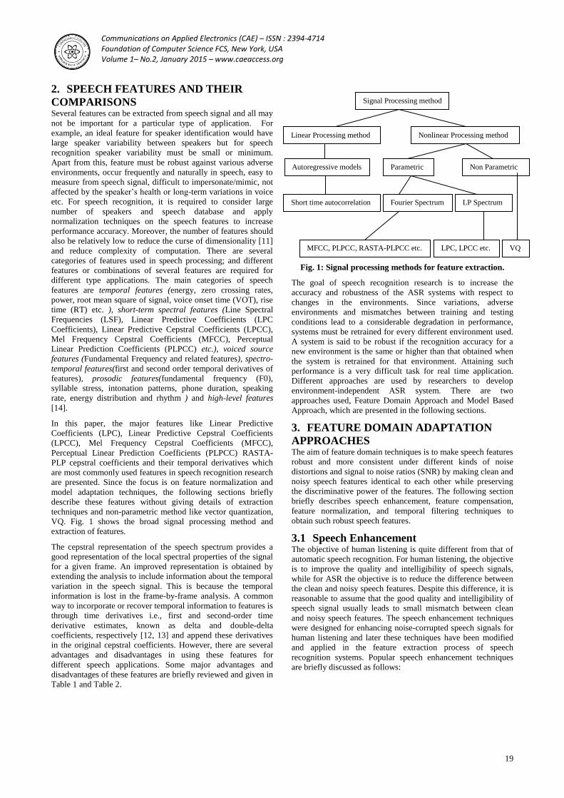
VQ. Fig. 1 shows the broad signal processing method and

extraction of features.

The cepstral representation of the speech spectrum provides a

good representation of the local spectral properties of the signal

for a given frame. An improved representation is obtained by

extending the analysis to include information about the temporal

variation in the speech signal. This is because the temporal

information is lost in the frame-by-frame analysis. A common

way to incorporate or recover temporal information to features is

through time derivatives i.e., first and second-order time

derivative estimates, known as delta and double-delta

coefficients, respectively [12, 13] and append these derivatives

in the original cepstral coefficients. However, there are several

advantages and disadvantages in using these features for

different speech applications. Some major advantages and

disadvantages of these features are briefly reviewed and given in

Table 1 and Table 2.

Fig. 1: Signal processing methods for feature extraction.

The goal of speech recognition research is to increase the

accuracy and robustness of the ASR systems with respect to

changes in the environments. Since variations, adverse

environments and mismatches between training and testing

conditions lead to a considerable degradation in performance,

systems must be retrained for every different environment used.

A system is said to be robust if the recognition accuracy for a

new environment is the same or higher than that obtained when

the system is retrained for that environment. Attaining such

performance is a very difficult task for real time application.

Different approaches are used by researchers to develop

environment-independent ASR system. There are two

approaches used, Feature Domain Approach and Model Based

Approach, which are presented in the following sections.

3. FEATURE DOMAIN ADAPTATION

APPROACHES The aim of feature domain techniques is to make speech features

robust and more consistent under different kinds of noise

distortions and signal to noise ratios (SNR) by making clean and

noisy speech features identical to each other while preserving

the discriminative power of the features. The following section

briefly describes speech enhancement, feature compensation,

feature normalization, and temporal filtering techniques to

obtain such robust speech features.

3.1 Speech Enhancement The objective of human listening is quite different from that of

automatic speech recognition. For human listening, the objective

is to improve the quality and intelligibility of speech signals,

while for ASR the objective is to reduce the difference between

the clean and noisy speech features. Despite this difference, it is

reasonable to assume that the good quality and intelligibility of

speech signal usually leads to small mismatch between clean

and noisy speech features. The speech enhancement techniques

were designed for enhancing noise-corrupted speech signals for

human listening and later these techniques have been modified

and applied in the feature extraction process of speech

recognition systems. Popular speech enhancement techniques

are briefly discussed as follows:

Signal Processing method

Linear Processing method Nonlinear Processing method

Autoregressive models Parametric Non Parametric

Short time autocorrelation Fourier Spectrum LP Spectrum

MFCC, PLPCC, RASTA-PLPCC etc. LPC, LPCC etc. VQ


20

Table 1. Comparisons of feature vectors (LP Coefficients, LPCC, MFFCC, PLP, RASTA-PLP and wavelet)

Features Advantages Disadvantages

LPC

&

LPCC

LPC is a production based method and it provides good model of

vocal tract characteristics. It represents the spectral envelope by low

dimension feature vectors and provides linear characteristics.

LPC is analytically tractable model. It is mathematically precise and

straight forward to implement in either software or in hardware.

The LP models the input signal with

constant weighting for the whole frequency

range. However, human perception does

not have constant frequency perception in

the whole frequency range.

Another serious problem with the LPC is

that they are highly correlated but it is

desirable to obtain less correlated features

for acoustic modeling. Other inherent

drawback of conventional

LPC analysis is its inability to include

speech specific a priori information in the

modeling process.

MFCC

MFCC is perception based feature. MFCCs are derived from the

power spectrum of the speech signal, while the phase spectrum is

ignored. This is done mainly due to our traditional belief that the

human auditory system is phase deaf, i.e., it ignores phase spectrum

and uses only magnitude spectrum for speech perception. MFCC

features are advantageous as it mimics some of the human

processing of the signal. Characteristics of the slow varying part are

concentrated in the low cepstral coefficients. Individual features of

MFCC are weakly correlated which turns out to be an advantage for

the creation of statistical acoustic model.

MFCC features give good discrimination and lend themselves to a

number of manipulations. It is capable of capturing the phonetically

important characteristics of speech.

Also band-limiting can easily be employed to make it suitable for

telephone applications. It has the basic desirable property that the

coefficients are largely independent, allowing probability densities to

be modeled with the diagonal covariance’s metrics.

Mel scaling has been shown to offer better discrimination between

phones, which is an obvious help in recognition.

A small drawback is that MFCCs are more

computationally expensive than LPCC due

to the Fast Fourier Transform (FFT) at the

early stages to convert speech from the

time to the frequency domain. First, they do

not lie in the frequency domain. Secondly,

as most current HMMs use Gaussian

distributions with diagonal covariance

matrices, these HMMs cannot benefit from

cepstral weighting. However, it is well-

known that MFCC is not robust enough in

noisy environments, which suggests that

the MFCC still has insufficient sound

representation capability, especially at low

SNR.

Though MFCCs have been very successful

in speech recognition, they have the

following two problems: (1) They do not

have any physical interpretation, and (2)

Liftering of cepstral coefficients, found to

be highly useful in the earlier dynamic

warping-based speech recognition systems,

has no effect in the recognition process

when used with continuous. The features

derived from either the power spectrum or

the phase spectrums have the limitation in

representation of the signal.

PLP

The PLP method takes advantage of three principal characteristics

derived from the psychoacoustic properties of the human hearing

viz., spectral resolution of the critical band, equal loudness curve

adjustment and application of intensity-loudness power law which

make it more effective than LPCC.

It approximates the speaker independent effective second formant. It

emphasizes first two formants F1 and F2 and deemphasizes high

frequencies in contrast with LP which emphasizes high frequencies,

F3. It reduces disparity between voiced and unvoiced speech. PLP

peaks are relatively insensitive to vocal tract length and PLP

estimates are highly correlated with the relatively speaker

independent front of the vocal tract. It reduces the sensitivity of ASR

front ends to changes in high frequencies and increases the

sensitivity to changes in F2 and F1.

It is computationally efficient and it yields a low-dimensional

representation of the speech. It is based on short term spectrum of

the speech. However, PLP technique is vulnerable when the short

time spectral values are modified by the frequency response of the

communication channel.

Computational requirements of PLP are comparable to their

conventional LP analysis. The advantage of the PLP technique over

the conventional LP is that it allows for the effective suppression of

the speaker-dependent information by choosing the particular model

One of weak points of PLP analysis is the

dependency of the result on the overall

spectral balance on formant amplitudes.

The spectral balance is easily affected by

factors such as the recording equipment,

the communication channel or additive

noise. The effect of the overall spectral

balance, to some extent, can be suppressed

a posterior by a proper distortion measure.

Just like most other short-term spectrum

based techniques this method is vulnerable

when the short-term spectral values are

modified by the frequency response of the

communication channel.


21

order. PLP features are advantageous as it also mimics some of the

human processing of the signal.

RASTA-

PLP

In ASR the task is to decode the linguistic message in speech. This

linguistic message is coded into movements of the vocal tract. The

speech signal reflects these movements. The rate of change of non-

linguistic components in speech often lies outside the typical rate of

change of the vocal tract shape.

The RASTA (relative spectral transform) takes the advantage of this

task. It suppresses the spectral components which change more

slowly or quickly than the typical range of change of speech. It

improves the performance of a recognizer in presence of convolution

and additive noise.

It is also used for enhancement of noisy speech. It makes the

recognizers much more robust to factors like choice of the

microphone or even to the microphone position relative to the mouth

that compare to short term spectrum based methods.

RASTA was developed to make PLP more robust to linear spectral

distortions. It takes advantage of the fact that the temporal properties

of environmental effects such as noise, distortions and convolution

are quite different from the temporal properties of speech.

The RASTA filter can be used either in the log spectral or cepstral

domains. In fact the RASTA filter band passes each feature

coefficient.

Linear channel distortions appear as an additive constant in both the

log spectral and the cepstral domains. The high-pass portion of the

equivalent band pass filter alleviates the effect of convolutional noise

introduced in the channel. RASTA-PLP is quiet efficient in dealing

with convolution noise. It is advantageous where the channel

conditions are not known a priori or where the channel conditions

may change unpredictably during the use of the recognizer.

A possible shortcoming of the non

inclusion of Linear Discriminant Analysis

(LDA) in RASTA-PLP is that the

quantization effect took effect before the

computation of LDA matrices.

LDA attempts to maximize the linear

separability between data points belonging

to different classes in the low-dimensional

representation of the data.

Wavelet

Due to the efficient time frequency localization and the multi-

resolution characteristics of the wavelet representations, the wavelet

transforms are quite suitable for processing non stationary signals

such as speech.

In wavelet analysis one can look signals at different scales or

resolutions: a rough approximation of the signal might look

stationary, while at detailed level discontinuities become apparent.

One major advantage afforded by wavelets is the ability to perform

efficient localization in both time and frequency.

The multi-resolution property of wavelets that can decompose the

signal in terms of the resolution of detail makes analysis capable of

revealing aspects of data that other signal analysis techniques miss

aspects like transients, breakdown points, discontinuities in higher

derivatives and self similarity.

Wavelet analysis can often compress or de-noise a signal without

appreciable degradation. Wavelets can zoom in to time

discontinuities and those orthogonal bases, localized in time and

frequency can be constructed.

Wavelet transforms have advantages over traditional Fourier

transforms for representing functions that have discontinuities and

sharp peaks, and for accurately deconstructing and reconstructing

finite, non-periodic and/or non-stationary signals.

Hence, wavelet transform is well suited to transient signals whose

frequency characteristics are time varying, especially like speech.

Wavelet method is non-adaptive because

the same basic wavelets are used for all

data.

Table 2. Different features, their parameters for different speech applications.

Types of Recognition Features

Isolated digit recognition MFCC + Energy + Derivatives

CSS MFCC + Energy + Derivatives

IWCSR LP Coefficients, LPCC + Derivatives

RCSR LPC + Derivatives

CWR MFCC + Energy + Derivatives

CSR LPCC + Derivatives

IWR MFCC + Derivatives


22

RSR isolated and connected MFCC + Energy + Derivatives

LVCSR MFCC + Energy + Derivatives

Phoneme Recognition MFCC + Energy + Derivatives

Isolated noisy Digit recognition MFCC + Energy + Derivatives or RASTA-PLP

NSR MFCC + Energy + Derivatives + RASTA-PLP

RSSR in noisy (IWR/CS) MFCC + LPC + Zero Crossing with peak amplitudes or RASTA-PLP

SSR MFCC + Derivatives Abbreviations used: CSS: Continuous Spontaneous Recognition, IWCSR: Isolated Word continuous Speech Recognition, RCSR: Robust

Continuous Speech Recognition, CWR: Continuous word Recognition, CSR: Continuous Speech Recognition, IWR: Isolated Word Recognition, RSR:

Robust Speech Recognition, LVCSR: Large Vocabulary Continuous Speech Recognition, NSR: Noisy Speech Recognition, RSSR: Robust Spontaneous Speech Recognition, SSR: Spontaneous Speech Recognition [102].

3.1.1 Spectral Subtraction Spectral subtraction is a simple but an effective way to reduce

additive noise's effects in speech signal. Spectral subtraction

estimates the clean speech spectrum by subtracting the estimated

additive noise spectrum from the noisy speech spectrum [20,

22]:

222^

|)(||)(||)(| kNkYkX (1)

where 2^

|)(| kX is the estimated clean speech spectrum, |(Y(k)|2

is the observed noisy speech spectrum, |N(k)|2 is the estimated

noise spectrum, and k is the frequency bin index. Spectral

subtraction is motivated by the fact that the noise corruption is

additive in the power spectrum domain, in expected sense if the

noise has zero mean in time domain, and is assumed to be

independent from the speech, i.e.

E[|Y(k)|2]=E[|X(k)+N(k)|2]=E[|X(k)|2]+E[|N(k)|2] (2)

where E[] denotes expected value. The performance of spectral

subtraction is directly affected by the accuracy of noise

estimation, which is a very difficult task by itself. In some cases,

the noise estimate |N(k)|2 is even larger than the noisy speech

|Y(k)|2, hence the estimated clean spectrum will be negative.

When this happens, the value of clean spectrum is usually set to

zero. This simple solution results in non natural spectral vectors

and causes “musical noise" phenomenon, which is annoying for

human listening and degrades speech recognition performance.

There are several kinds of spectral subtraction, and they mainly

differ in the way to handle the “musical noise". In [23], over

subtraction and spectral floor are used to provide a tradeoff

between the “musical noise" and residual noise level. In [24], it

is proposed to apply the masking properties of ear to determine

the amount of subtraction. The basic idea is that for those noise

components that cannot be heard by a human ear, it is not

subtracted, so there is a smaller amount of subtraction and

therefore smaller degree of distortion. Despite its application in

enhancing speech for hearing, spectral subtraction has also been

used to preprocess noisy speech in the feature extraction process

of speech recognition systems [25]. The limitation of spectral

subtraction is that it aims to reduce noise distortion in the signal

domain and has no direct relationship with the final speech

recognition task, i.e. to achieve high recognition accuracy. In

addition, spectral subtraction's performance depends heavily on

the accuracy of noise estimation which is difficult especially

when the noise is non-stationary and has similar characteristics

as speech signal, such as babble noise.

3.1.2 MMSE Spectral Magnitude Estimator. A more advanced speech enhancement technique than spectral

subtraction is the optimal estimator of speech's short-time

spectral amplitude (STSA) in the minimum mean square error

(MMSE) sense [27, 28]. In the MMSE STSA estimator, the

phase and amplitude of spectral components of clean speech

signal and noise are assumed to be independent Gaussian

variables. With this assumption, the distribution of the spectral

component of noisy speech signal follows the Rayleigh's

distribution. The MMSE estimate of the clean spectral amplitude

is then derived based on these models, and the resulting solution

of the estimator is a function of the a priori SNR and the a

posteriori SNR of the speech signal. The a priori SNR is the

expected SNR before the current frame is observed. It is critical

for the performance of MMSE STSA estimator and can be

estimated using either Maximum Likelihood estimation or a

“decision-directed" method. The a posteriori SNR is the

instantaneous SNR of the current frame. Several methods have

been proposed to improve the accuracy of the estimate of the a

priori SNR. Some researchers focused on improving the average

weighting parameter α of the decision directed method [27, 28],

which controls the speed of adaptation. Soon and Koh [29]

proposed to estimate α from the changing speed of frame

energy. This idea is further extended in [30] by using a

frequency-dependent MMSE estimator of α. Besides the

estimation of α, to incorporate more information, Israel [31]

proposed a non causal a priori SNR estimator that employs both

past and future frames for better estimation. Another approach

by Hu and Loizou [32] reduces the variance of the a priori SNR

estimate indirectly by reducing the variance of noise estimate.

Another important characteristic of the MMSE STSA estimator

that incorporates a signal absence probability (SAP) was

introduced by McAulay and Malpass [21]. With SAP, the

estimate of a clean speech becomes:

)())(|()(^^

kXkYpresentSpeechPkX MMSE (3)

where P(speech present|Y(k)) is the posterior probability of

speech present at the kth frequency bin when noisy spectral

coefficient Y(k) is observed, and )(^

kX MMSE is the MMSE

estimation of clean spectral coefficients. Later, the MMSE

estimator of STSA was extended to log spectral domain [28] to

simulate the nonlinear compression of the human auditory

system. The MMSE STSA have been successfully applied to

noisy speech recognition tasks, e.g. in [33, 34].

3.1.3 Subspace-based Techniques. Another popular speech enhancement technique is the signal

subspace method, which is motivated by the fact that noisy

speech signal can usually be decomposed into two subspaces:

the signal plus noise subspace and the noise only subspace.

During the enhancement process, the noise only subspace can be

removed completely and the clean speech signal can be

estimated from the signal plus noise subspace. There are two

methods to decompose the noisy signal into the two subspaces,

namely the singular value decomposition (SVD) method and the

Karhunen-Loeve transform (KLT). In the SVD-based method

[35], the clean signal is reconstructed from the singular vectors

corresponding to the largest singular values. It is believed that

the singular vectors corresponding to the largest singular values


23

contain speech information, while the singular vectors

corresponding to the smallest singular values contains noise

information. This approach provides large SNR gains for speech

corrupted by white noise. In the Quotient SVD-based approach

proposed by Jensen et al [36], the previous approach is extended

to suppress colored noise. However, QSVD is computationally

expensive.

Many approaches also use KLT to decompose noisy signal. In

Ephraim and Van Trees’ method [37], the estimator minimizes

speech distortion subject to a given residual noise level

constraint. In this way, a mechanism is provided to adjust the

tradeoff between the signal distortion and the residual noise

level. Huang and Zhao [38] extended the method of Ephraim

and Van Trees by proposing an energy-constrained signal

subspace method (ECSS). The idea was to match the short-time

energy of enhanced speech signal to the unbiased estimated of

the clean speech. They declared that this method recovered the

low-energy segments in continuous speech effectively. Rezayee

and Gazor [39] proposed an algorithm to reduce colored noise

by diagonalizing the noise correlation matrix using the estimated

Eigen values of the clean speech and nulling any off-diagonal

elements. Mittal and Phamdo [41] also extended method of

Ephraim and Van Trees to colored noise by providing proper

noise shaping for colored noise without pre-whitening. One

important assumption of signal subspace approach is that the

largest singular values or Eigen values are from speech and the

smallest values are from noise. In [40] several subspace-based

methods have been evaluated on noisy speech recognition task.

3.2 Feature Compensation Speech enhancement techniques try to recover the time domain

speech signal for human hearing but in feature compensation

methods the aim is to recover clean speech coefficients from

noisy speech coefficients during the feature extraction process of

speech recognition without generating corrected speech signal in

time domain. There are another two major differences between

these two groups of methods. One difference is that speech

enhancement techniques usually operate in time domain,

frequency domain or log frequency domain, while feature

compensation methods usually work in the log filter bank

domain or cepstral domain. Another difference is that feature

compensation methods are solely designed for noisy speech

recognition tasks, while speech enhancement methods are

originally proposed to improve speech signal for human

listening. Feature compensation methods can be classified into

two groups based on whether they use the environment model

described in the following sections: i.e. model-based approach

and data-driven approach.

3.2.1 Model-based Feature Compensation An early model-based feature compensation technique is the

code-dependent cepstral normalization (CDCN) [42]. The clean

cepstral vector x are modeled by a Gaussian mixture model

(GMM). The CDCN estimates the clean cepstral vectors from

the noisy observations in the MMSE sense. The closed-form

solution of the MMSE estimator of x is:

M

i

iryiphyx1

^^^

)()|( (4)

where^

x and^

h are the estimate of the clean cepstral vector and

channel distortion, respectively. y is the noisy cepstral vector,

p(i|y) is the posterior probability of the ith mixture in the GMM

after y is observed, M is the number of mixtures, and )(^

ir is the

codeword-dependent correction vectors that need to be

estimated. In CDCN phase insensitive environment model is

used. It is to be observed that the GMM of the clean cepstral

vector x are first adapted to noisy GMM using estimated noise

and channel distortions and environment model, then p(i|y) for

all mixtures are calculated.

The noise and channel distortions are estimated using the ML

criterion as there is usually no prior information about them

available. The distortions are assumed to be constant during the

analysis duration, e.g. an utterance. By assuming speech frames

to be independent from each other, the log likelihood of the

training data is:

T

t

t hnyphnYp1

),|(log),|(log (5)

where Y = y1,…yT is the feature vector sequence of an utterance,

n is the noise distortion and T is the number of frames in the

utterance to be processed. In [42], the distribution p(y|n, h) is

obtained by using the environment model and the distribution of

x with some assumptions. The optimization is implemented

using the expectation maximization (EM) algorithm [43].

Another model-based feature compensation method is proposed

by Deng et. al. in [44 - 46]. A major difference between Deng's

estimator and CDCN is that the phase sensitive environment

model is used in Deng's estimator for more accurate modeling of

speech-noise relationship. Besides, Deng's estimator operates in

the log Mel filterbank domain, while CDCN is a cepstral

coefficients estimator. Similar to CDCN, there are two major

parts in Deng's estimator, i.e. the MMSE estimation of the clean

speech feature vector based on the adopted environment model

and the prior probability distribution of clean speech, and the

estimation of noise distortion. The GMM is also used for clean

feature vector modeling in Deng's estimator. The phase factor is

also modeled as zero-mean Gaussian distributed. With this prior

distribution of clean speech, phase, and the phase-sensitive

environment model, the MMSE estimator of clean feature vector

can be obtained. However, the estimator is too complex and

needs to be simplified by using the second-order Taylor series

expansion. Channel distortion is ignored and sequential noise

estimation [20] is used to track additive noise. In addition, the

assumption of stationary noise in CDCN is removed in Deng's

estimator. It was found by Deng et. al. that the recognition

performance of the phase-sensitive MMSE estimator [44] was

better than that of the phase-insensitive MMSE estimator in [48]

with 54% error rate reduction. This shows that the incorporation

of the phase information benefits the feature compensation

process by including relevant information. If the phase factor is

set to zero, the phase-sensitive MMSE estimator degenerates to

spectral subtraction. Later, the phase-sensitive MMSE estimator

is expanded to include the first order derivatives of the speech

features in the log Mel filterbank domain [45], due to the

assumption that the strong dynamic property of speech features

are important for the enhancement of the features. The static and

dynamic features are assumed to follow a GMM distribution and

be independent from each other. Then the noisy speech feature

distribution function is derived and the clean speech features are

estimated using the MMSE criterion. The work of Deng et. al.

was further expanded by incorporating a feature compensation

uncertainty [46] in the decoding process. The feature

compensation uncertainty accounts for the deviation of the

enhancement feature from the clean feature, i.e. the variance of

the feature estimator. To better decode the noisy speech, this

uncertainty should be taken into account in the decoding

process. One way to do this is to integrate the acoustic score


24

over this uncertainty space, i.e. over all possible clean feature

values. One issue for incorporation of the uncertainty is how to

efficiently calculate the integration. The integration is

effectively the same as adding the variance of the feature

estimator (the uncertainty) to the Gaussian's of the HMM states

if the feature estimation error is assumed to be zero-mean

Gaussian distribution [46]. Another issue is how to effectively

estimate the feature estimator's variance. In [19], analytical

solutions are derived by making use of the phase-sensitive

environment model.

3.2.2 Data-driven Feature Compensation The simplest data-driven feature compensation is the cepstral

mean normalization (CMN) [12]. In CMN, the features are

compensated as:

ryx tt ^

(6)

where ^

tx and yt are the estimated clean feature vector and

noisy feature vector for the tth frame respectively, and r is the

correction term that is the mean of the features, usually obtained

by averaging the feature vectors over an utterance. The mean of

features is in fact the optimal estimate of the correction term r in

the MMSE sense if only a single correction vector is allowed

[49]. The operation of CMN to compensate all feature vectors

by a single fixed correction vector is too limiting. The use of a

single vector r can only compensate for convolutional noise in

the feature domain. In [50], a method called multivaRiate

gAussian-based cepsTral normaliZation (RATZ) is proposed to

use multiple correction vectors. In RATZ, the clean feature

space is modeled by a GMM. The distribution of the noisy

speech is also assumed to be GMM. It is observed that in the log

Mel filterbank and cepstral domain, the effect of noise on the

distribution of speech signal is that the mean is shifted and the

variance is either decreased or increased depending on the SNR.

Therefore, the noisy GMM can be approximated by adding a

correcting term to the mean and variances of the clean GMM.

Let the distribution of the cepstral vectors of the clean and noisy

speech be GMM with the same number of mixtures

),()()(1

i

x

i

xx

M

i

Nipxp (7)

),()()(1

i

y

i

yy

M

i

Nipyp (8)

where i

y

i

y , represent mean and variance of vectors. The

noisy distribution function can be approximated by adding

correction terms to the clean mean and covariance parameters

Mir ii

x

i

y ,....,1, (9)

MiRii

x

i

y,....,1, (10)

The correction terms are estimated based on the maximization of

the likelihood for the noisy observation. As there is no closed-

form solution for the correction terms, the EM algorithm is

applied again. After the ri and Ri are obtained, the RATZ

estimates the clean cepstral vector using the MMSE criterion as

follows:

M

i

ii

y

i

y ryipyx1

^

),,|( (11)

which is a weighted sum of mean correction vectors ri. The

correction vectors ri and Ri can also be used to adjust the

parameters of acoustic models for better match between the

model and noisy data. The estimated noisy mean and variance

are used to evaluate the posterior of mixtures. For more detail,

interested reader may refer [51-54].

3.3 Feature Normalization Unlike speech enhancement and feature compensation methods

that aim to recover the clean speech coefficients, the feature

normalization methods normalize the speech coefficients,

usually cepstral coefficients, to a new space where the noise

distortion is reduced. It should be mentioned that both the

compensation and normalization methods modify feature vectors

and thus the difference between them is not very clear, however,

feature normalization methods usually modify certain statistics

of features, e.g. global means and variances, to some reference

values which are usually obtained from clean speech or simply

pre-defined values. A rationale of doing so is that the statistics

of speech features are changed when speech signal is distorted

by noise. By normalizing the statistics of the speech features, it

is expected that some systematic distortion caused by noise will

be reduced. In this section, major feature normalization methods

are reviewed.

3.3.1 Cepstral Mean and Variance Normalization A simple and effective feature normalization method is the

cepstral mean normalization (CMN), also called cepstral mean

subtraction (CMS) [12, 55]. The CMN is already introduced as a

data-driven feature compensation method in above section.

However, it can also be treated as a feature normalization

method. CMN subtracts the features' mean values from the

features. After subtraction, all the feature dimensions will have a

zero mean. It is known to be able to reduce the convolutional

noises, such as microphone mismatch and linear transmission

channels distortion. This is because convolutional noises

becomes multiplicative in the frequency domain and additive in

the log filterbank and cepstral domain. If the convolutional noise

is fixed, it causes a constant shift in the log filterbank and

cepstral domain. Therefore, by subtracting the mean from the

feature for both clean and noisy speech, the convolutional noise

can be removed in theory. The basic CMN [12, 55] estimates the

sample mean vector of the cepstral vectors of a sentence and

then subtract this mean vector from every cepstral vector of the

sentence. An augmented cepstral normalization method [42]

estimates the mean vectors for the silence and speech segments

of the sentence separately and achieved better results. Instead of

using a hard decision on whether a frame is silence or speech,

one improvement suggests the use of the a posteriori probability

of the frame of being silence p(n), which is similar to the speech

absence probability used in the MMSE STSA. The final mean

vector is the weighted sum of the silence mean and speech

mean, with the weights be p(n) and 1-p(n) respectively. In

another study [56], CMN is also used together with microphone

array and is called position-dependent CMN. The speaker's

position is first estimated by the microphone array, and then a

pre-trained feature mean for the location is used to perform

CMN. In general, the advantage of CMN is its simplicity, low

computational cost and easy to be implemented. However, its

performance is limited as it uses very few items of prior

information about speech and noise, and the use of a single

compensation vector provides very little flexibility. Besides

mean normalization, the cepstral variance normalization (CVN)

[57] normalizes the variances of features to unity. It is well

known that noise distortion can change the variance of speech

features. At different SNR levels, the variance of features may


25

be very different. The CVN is similar to a dynamic gain control.

It normalizes the total power of feature trajectories to reduce the

difference among features of different environmental conditions.

In practice, CMN and CVN is normally used in cascade and

called the mean and variance normalization (MVN).

3.3.2 Histogram Normalization Histogram Equalization (HEQ) is also used for normalization.

While CMN and CVN normalize the first and second moments

of features respectively, histogram equalization [58, 59]

normalizes the histogram of the features, i.e. the probability

density function (p.d.f.) of the features. Originally used in image

processing to automatically balance the contrast of images, HEQ

is a technique that can change the histogram of any random

variable to match any other desired histogram. For a random

variable x with known cumulative distribution function (cdf) Cx,

we can change its cdf to Cy by performing

))((1 xCCy xy

(12)

where y is the transformed version of x. In speech recognition

systems, HEQ can be applied to normalize the distribution of

speech features. A reference histogram is first learnt from the

training data of acoustic model. Then the histogram of the test

features is normalized towards this reference histogram. The

process is performed on a dimension-dependent and utterance

wise basis. Besides histogram of training data, common

probability distributions can be used, such as Gaussian

distribution, as the reference. Usually, both the training and

testing features are processed by HEQ. HEQ can be seen as a

generalization of CMN and CVN, since when the histogram

(p.d.f.) of features are normalized, all moments should be

normalized. From another viewpoint, CMN and CVN provide a

linear transformation of the features, while HEQ is able to

transform the features nonlinearly.

The CMN, CVN/MVN, and HEQ all have two assumptions, i.e.

the assumption that the noise distortion does not change the

order statistics of feature trajectories within an utterances or

segment; and global statistics of an utterance match that of the

whole training set. The order statistics of a feature trajectory

refers to which element of the trajectory has the highest value,

the second highest value, and so on. In fact, noise distortion

usually breaks this order. Hence, even if we can normalize the

histogram of the noisy trajectory to the histogram of

corresponding true clean trajectory, the normalized trajectory

won't be the same as the clean trajectory. Besides this

assumption, the assumption about matched statistics is also

violated in real situations. In training data, we have a balanced

proportion of all the phonemes. However, during testing, as

there is very limited number of phonemes in an utterance, the

phoneme composition of an utterance may be quite different

from that of the training set. Hence, it is coarse to normalize the

histogram of just one utterance to the global histogram of the

entire training set which usually consists of thousands of

utterances. There is another simple example to demonstrate the

drawbacks of CMN, CVN, and HEQ [61]. Suppose there is an

utterance with several words. If several silence frames are

appended in both the front and end of the utterance, another

utterance is obtained. Although the acoustic content of these two

utterances are exactly the same, their normalized versions by

CMN, CVN/MVN, and HEQ will be different due to the

different proportions of silence frames in the two utterances. The

violated assumptions of CMN, CVN, and HEQ are alleviated by

the use of cluster based normalization techniques. In [60], a

more general solution is proposed, i.e. the class-based HEQ. In

this method, the clean training feature vectors are first clustered,

and then a reference histogram is estimated for each cluster.

During recognition, the noisy feature vectors are first classified

into clusters, and then the conventional HEQ is performed for

each cluster independently. With class-based HEQ, it is possible

that the order statistics of the normalized feature vectors will be

different from that of the original vectors. Although this does

not guarantee that the order statistics of the normalized features

will be more like the corresponding clean features.

3.4 Temporal Filtering Filtering of feature trajectories is also a popular approach to

improve the robustness of speech recognition against noise

corruption. Typically, the filtering is applied to the trajectories

of log filterbank coefficients or cepstral coefficients, which are

treated as time domain signals. The filters are usually called

temporal filters. The most significant difference between

temporal filters and previous feature domain methods are that

the temporal filters modify the correlation of features, i.e.

second order statistics of features or modulation spectrum, while

previous methods modify the probability distribution of features,

i.e. first order statistics of features.

A common temporal filtering technique is the extraction of

delta and acceleration features [95]. The delta and acceleration

(delta-delta) features are generated using the expression

M

Mm

M

Mm

m

mtmxtx

dt

dtx

2

)()()(

(13)

where 2M+1 is the number of frames considered in the

evaluation. The same formula can be applied to the first order

derivative to produce the second order derivative. The delta

features are seen as band-pass filtered versions of the static

features. This can be seen as a finite impulse response (FIR)

filter. The delta filter is a band-pass filter with the center of

passband near 15Hz modulation frequency. Delta and

acceleration features are usually appended to the static features

and they are shown to improve the performance of speech

recognition significantly. The CMN discussed above, can also

be treated as a temporal filter. Strictly speaking, the magnitude

response of CMN is time-varying and can only be roughly seen

as a highpass fillter. CMN eliminates the very low frequency

components of feature trajectories that could be caused by but

not limited to channel distortions.

The first commonly used temporal filter specifically designed

to reduce the effect of channel distortion and additive noise is

the RASTA filter (relative spectra) [96]. The RASTA filter is an

IIR filter whose transfer function is defined as:

1

4314

1

221.0)(

pz

zzzzzHRASTA

(14)

where p is a parameter controlling the cut-off frequency of the

high-pass portion of the filter. Typically, p is set to either 0.98 or

0.94 [96].. It is a bandpass filter that removes the very low

frequency and high frequency components of feature

trajectories. The design agrees with research findings that

speech modulation frequency of 1-16Hz is most important for

both human and automatic speech recognition [62-68]. RASTA

and CMN are both able to reduce channel distortions, and they

can be used in concatenation to produce better results.

Another well-known temporal filter designed to reduce

feature variation is the autoregressive moving average (ARMA)

filter used in the MVA processing [97]. The ARMA filter is

defined as:

12

)(...)()1(...)1()()(

M

MtxtxtyMtyMtyty

(15)


26

where x(t) and y(t) are the input and output of the filter, M is the

order of the filter. The transfer function is:

)12/()...(1

...1

12)(

21

1

Mzzz

zz

M

zzH

M

MM

ARMA

(16)

The larger the filter orders M, the lower the cut-off frequency of

the ARMA filter. The optimal value of M is usually dependent

on the task. Besides the empirically designed temporal filters

such as RASTA and ARMA, some researchers also propose to

use data-driven methods for filter design [69-73]. The filters are

usually designed from some training data which can be both

clean and noisy. Typically, discriminative criteria are used to

guide the filter design, e.g. linear discriminative analysis (LDA)

and minimum classification error (MCE). Besides, principle

component analysis has also been used. The filter parameters are

estimated by optimizing the objective function of these criteria.

The resulting filters are mostly low-pass or band-pass, similar to

RASTA and ARMA filters.

Most of current temporal filters are fixed after being designed.

They are not able to track the changes of signal condition during

speech recognition.

4. MODEL ADAPTATION TECHNIQUES In contrast to feature domain methods that aim at making

features more consistent in various environmental conditions,

the model adaptation methods adapt acoustic model to make it

better fit to the noisy acoustic environment. Several model

adaptation techniques are briefly reviewed and compared in the

following sub sections. These methods are grouped into data-

driven-based adaptation and environment-model-based

adaptation based on whether environment model is used or not.

4.1 Data-driven-based Adaptation There are several data-driven based adaptations like STAR,

Stochastic Mapping, MAP and MLLR, and Ensemble modeling.

They are briefly reviewed in the following sections.

4.1.1 STAR. The STAR algorithm of Moreno [50] is closely related to the

RATZ feature compensation algorithm described in section 3.2.

Feature compensation methods usually have a model adaptation

counterpart. The basic concept of STAR is similar to that of

RATZ. However, unlike RATZ which uses a separate GMM for

the prior distribution of clean speech, STAR utilizes the HMM.

STAR estimates the correcting terms, μk and ∑k, for the 256

Gaussians using the same way as RATZ, and then compensates

the clean mean and variance vectors to approximate the noisy

speech distribution [50]. As these Gaussians are shared by all

HMM models, once they are compensated, all the HMM states

are adapted.

4.1.2 Stochastic Mapping In stochastic matching, it is assumed that the matched acoustic

model can be adapted from the clean-trained acoustic model by

)( xy G (17)

where Gη() is the transformation function and η is its parameters.

In [74], the transformation function is assumed to be:

bxy (18)

bxy (19)

where μb and ∑b are the correction mean and variance and they

are estimated for every Gaussian in the acoustic model. In

RATZ and STAR, the same type of correction vectors is

assumed to estimate noisy speech distribution from clean

distribution. The difference is that in stochastic matching, the

model is HMM rather than GMM. Similar to feature space

stochastic matching, the correction vectors are estimated by

maximizing the likelihood of noisy utterance

),|,,(maxarg),|(maxarg^

x

CS

x CSYpYp

(20)

where ˄x is the HMM-based acoustic model trained from clean

features, Y is the collection of feature vector for an utterance, S

and C are all possible state sequences and mixture sequences of

Y. The optimization can be solved by EM algorithm. The

stochastic matching was improved later by using nonlinear

mapping function in [75] and by an SNR-incremental stochastic

matching in [76].

4.1.3 MAP and MLLR Another two model adaptation methods, the maximum

likelihood linear regression (MLLR) [98] and maximum a

posteriori (MAP) [77, 78], have been originally designed for

adapting speaker independent acoustic models to a specific test

speaker. Due to the similarity between the speaker adaptation

and environment adaptation, they are also used for noise robust

speech recognition. The MAP approach adapts the acoustic

model by optimally using the prior information in the clean

trained acoustical model and the posterior information in the

noisy observations. The observations are recognized by speech

recognition, and only those with high acoustic likelihood score

are used for adaptation. The Bayesian adaptation framework

used in the MAP approach enables the optimal use of the noisy

observations in model adaptation. When the adaptation data are

few and the posterior information is weak compared to the prior

HMM acoustical models, the models are not adapted much. As

there are more and more adaptation data, the models becomes

asymptotically equivalent to the ML estimate from noisy

observations, which provides optimal decision rule on the test

data. However, this adaptation process is quite slow, as only the

model parameters directly related to the adaptation data are

adapted. In real applications, the adaptation data are few and

hence it is necessary to reduce the number of model parameters

needed to be adapted. To achieve good adaptation performance,

MLLR [98] uses the parameter sharing strategy, i.e., the similar

models are tied together and their parameters are adapted

together. The degree of model tying is high if the available

amount of adaptation data is low and vice versa. For very few

data, a global transforms strategy may be used. The basic MLLR

adapts the mean vectors of the Gaussian by multiplying it with a

transform matrix, which is obtained using maximum likelihood

criterion and EM algorithm. The models tied together share the

same transformation matrix. The advantage of the MLLR is its

ability to provide good adaptation even if data are few.

However, MLLR has poor asymptotic properties, which leads to

the fast saturation of performance gain with increased data.

Researchers found that the MLLR usually outperforms the MAP

if the adaptation data are few, but MAP adapts the models better

when there are a lot of data and the combination of the two

methods yields better performance.

4.1.4 Ensemble Modeling In practice, there is often very little or no data for supervised

adaptation. Hence, it is important to reduce the number of free

parameters that need to be estimated during adaptation. In the

eigenvoice-based speaker adaptation method [81], the number of

free parameters is reduced to about 10 such that these

parameters can be estimated from limited data robustly. The

ensemble modeling can be seen as a generalization of the


27

eigenvoice approach for the environment-adaptation problem

[79, 80]. In the ensemble modeling approach, an ensemble of

acoustic models are trained using speech data of various

environment conditions, e.g. different noise and SNR

combinations. After obtaining P acoustic models, the mean

vectors of Gaussians in each model are concatenated to form a

supervector and there are totally P supervectors, one supervector

for one acoustic model. Each supervector has M x D

dimensions, where M is the number of Gaussian mixtures in an

acoustic model and D is the feature dimension. The idea is to

estimate a supervector from these P supervectors based on the

noisy observations. The estimated supervector can then be used

to construct an acoustic model for speech recognition. In its

most general form, the test supervector can be estimated as

follows:

P

p

pptest bsAs1

(21)

where tests

is the estimated supervector that is supposed to be

matched with the noisy test data, sp and Ap is the pth supervector

and transformation matrix, and b is a correction vector. The

transformation matrices Ap, p = 1,…,P and the correction vector

b can be estimated using the maximum likelihood criterion and

the noisy test data. If there is only one model in the ensemble,

i.e. P = 1, the approach degenerates to MLLR. A problem with

this general form is that there are too many parameters and it is

very difficult if not impossible to estimate these parameters

robustly. A practical form of ensemble modeling approach [79,

80] is as follows:

P

p

pptest sws1

(22)

where wp is a scalar weight rather than a transformation matrix.

In addition, the correction vector is removed. In this

formulation, the number of free parameters is P. To further

reduce complexity, K eigenvectors (K ≤ P) can be obtained by

PCA and used to replace sp in (22). In this case, there are only K

free parameters. It is reported in [61] that the ensemble

modeling approach outperforms MLLR significantly on Aurora-

2 task. Two extensions of ensemble modeling are reported in

[79]. The first extension is to use a tree-based clustering of the

environments. During testing, the environment is first estimated,

and only the supervectors of the selected environments are used

for adaptation. The second extension is to use minimum

classification error (MCE) criterion rather than ML [99, 100] to

obtain discriminative supervectors.

4.2 Environment Model-based Adaptation Another group of model adaptation methods uses the

information of the environment model. A very brief review of

such two popular methods, the Parallel Model Combination

(PMC) [82] and Joint Compensation of Additive and

Convolutive noise (JAC) [83] are given in the following

sections.

4.2.1 PMC Gales and Young [82] proposed the PMC approach, which

synthesizes a noisy acoustic model using clean acoustic model

and a noise model. In PMC, the noise is represented by a single

or multi-state HMM depending on whether the noise is

stationary. During the adaptation process, the noise model can

be trained from the frames of silence segments in the testing

utterances. Both the clean acoustic model and noise model are

trained from cepstral features; however, the noisy acoustic

model is synthesized in linear spectral domain, i.e. the filterbank

domain before natural logarithm and DCT. Therefore, it is

necessary to convert the mean and variance vectors of the clean

and noise models back to the linear spectral domain first. After

the noisy acoustic model is obtained in the linear spectral

domain, it is then converted to the cepstral domain and used for

speech recognition. The parameters of the clean acoustic model

are compensated by adding the parameters of the noise model in

the linear spectral domain. Specifically, for each clean and noise

state pair, the mean vectors and covariance matrices of the two

models are combined using the following formulae __

g (23)

___

2g (24)

where (

, ), (μ, ∑) are the noisy and clean speech model

parameters, ____

, are the noise model parameters, all in linear

spectral domain. The gain matching term g is used, as the

relative strengths of the speech and the noise in the testing

environment may be different from these training environments,

and it is estimated as

s

nns

E

EEg

(25)

where Es, Ens and En are the average energy of the clean speech,

noisy speech and background noise respectively. It is reported in

[82] that PMC significantly improves performance on isolated

digit recognition task.

4.2.2 JAC JAC [83] is another model adaptation method that uses an

environment model. Similar to PMC, JAC also transforms the

acoustic model's parameters back, but to log filterbank domain

rather than linear spectral domain. Furthermore, JAC deals with

both additive and convolutive noises, while original PMC only

compensate for additive noise. In JAC, the phase-insensitive

environment model is used. JAC first estimates the additive and

convolutive noises from the current noisy test utterance using an

EM algorithm. With these noise estimates, JAC adapts acoustic

model's parameter in the log filterbank domain, and then

converts the parameters back to cepstral domain. The adapted

model is used to decode the test utterance, and the output

alignment information is used to obtain a better estimation of the

channel distortion, which is used as the initial value for the

channel distortion for next test utterance. The additive noise

estimate of current utterance is not similarly used in next test

utterance as additive noise is assumed to be highly non-

stationary. There are two extensions to JAC [85, 86]. In the first

extension [85], vector Taylor series (VTS) is used to linearize

the nonlinear distortion in the environment model. Another

improvement is that the adaptation is now carried out in the

cepstral domain directly and there is no need to convert the

model parameters to log filterbank domain.

In addition, the extended JAC also adapts the Gaussian

variances of the acoustic model, which are not adapted in

original JAC. The second extension [86] is an improvement over

the first extension. The major improvement is that the phase-

insensitive environment model is replaced by the phase-sensitive

model for more accurate modeling of the relationship between

noises and speech. It is reported in [86, 103] that the use of a

phase-sensitive model significantly improves recognition

performance on the Aurora-2 task, where the data follows the

phase-sensitive model well.


28

5. THE HYBRID MODEL The speech recognition is a pattern recognition task and

Artificial Neural Network (ANN) is a good classifier. However,

Artificial Neural Networks are not very good at handling

dynamic data and speech signal is dynamic as it varies over time

as it progresses. Thus, with standard neural networks it is

difficult to handle this temporal variation in speech signals

uttered by different speakers or at different speaking rates.

Therefore, several researchers started combining elements of

HMMs and neural networks [87 - 91, 101]. Various components

of the HMM are implemented using neural networks to increase

the performance of HMM system. In [90] a special recurrent

neural network called a Viterbi Net was introduced as a way of

implementing the Viterbi algorithm for an HMM. In [91] a

similar model called recurrent AlphaNet, was introduced as a

way of implementing the forward recursions of an HMM.

Another very interesting neural network implementation of a

discrete HMM is the so called Boltzmann chain introduced in

[92]. The Boltzmann chain is a particular variant of Boltzmann

machine [93], which is very similar to the globally normalized

discrete HMM [93] that can be trained by a gradient-based

algorithm which has many similarities to gradient-based

forward-backward training for globally normalized HMMs.

So, rather than simply implementing the HMM alone, most of

the current researchers also focus on HMM-ANN hybrids, to

capitalize the strengths of each of the two frameworks: the

temporal modeling capabilities of the HMM and the static

classification or function approximation capabilities of Artificial

Neural Networks. This hybrid model is also a trend towards

efficient and robust system development in speech recognition

research. However, it still remains a big challenge for the

researchers to develop ASR system that gives 100% accurate

performance in mismatched environments or that matches the

performance of human counterpart.

6. CONCLUSION In this paper, major speech features used for speech recognition

and different environment adaptation techniques for

development for robust speech recognition system are reviewed.

Integration of two different modeling techniques of HMM and

Artificial Neural Networks to exploit the temporal modeling

capabilities of HMM and the static classification capabilities of

neural networks in order to construct robust speech recognition

system is also reported. This paper may be useful as a tutorial

and review on the state-of-the-art speech recognition systems,

feature normalizations/adaptations, model adaptation etc. for

students, scholars/researchers and other in the field of speech

recognition research. It will be helpful for researches and

development of robust ASR system in adverse environments.

7. REFERENCES [1] B. H. Juang, and Lawrence R. Rabiner. “Automatic Speech

Recognition – A brief History of the Technology

Development.”, Elsevier Encyclopedia of Language and

Linguistics, 2004.

[2] Sadaoki Furui. “50 Years of Progress in Speech and

Speaker Recognition.”, ECTI Transactions on Computer

and Information Technology, Vol. 1, No.2, November

2005.

[3] L. R. Rabiner and B. H. Juang. Fundamentals of Speech

Recognition, Prentice-Hall, Englewood Cliff, New Jersey,

1993

[4] Tomi Kinnunen, Haizhou Li, “Overview of text-

independent speaker recognition: From features to

supervectors.” Speech Communication, 52, pp. 12–40,

2010.

[5] D.S. Pallet, “Speech Results on Resource Management

Task,” in Proceedings of the February 1989 DARPA

Speech and Natural Language Workshop, Morgan

Kaufman Publishers, Inc., Philadelphia, PA, USA, pp. 18-

24, February 1989.

[6] D. Paul, “The Lincoln Robust Continuous Speech

Recognizer,” in Proceedings IEEE International

Conference on Acoustics, Speech, and Signal Processing,

pp. 556-559, Glasgow, Scotland, May 1989.

[7] J.G. Wilpon, R.P. Mikkilineni, D.B. Roe, and S. Gokcen,

“Speech Recognition: From the Laboratory to the Real

World,” AT&T Technical Journal, vol. 69, no. 5, pp. 14-24,

October 1990.

[8] J.G. Wilpon, D.M. DeMarco, R.P. Mikkilineni, “Isolated

Word Recognition Over the DDD Telephone Network -

Results Of Two Extensive Field Trials,” in Proceedings

IEEE International Conference on Acoustics, Speech, and

Signal Processing, pp. 55-57, New York, NY, USA April

1988.

[9] B. Wheatley and J. Picone, “Voice Across America: Toward

Robust Speaker Independent Speech Recognition For

Telecommunications Applications”, Digital Signal

Processing: A Review Journal, vol. 1, no. 2, p. 45-64, April

1991.

[10] Picone, J., “The Demographics of Speaker Independent

Digit Recognition”, in Proceedings IEEE International

Conference on Acoustics, Speech, and Signal Processing,

pp. 105-108, Albuquerque, New Mexico, USA, April 1990.

[11] Jain, A., Duin, R., Mao, J., “Statistical pattern recognition:

a review.” IEEE Transaction on Pattern Anal. Machine

Intelligence, 22 (1), 4–37, 2000

[12] Furui, S., “Cepstral analysis technique for automatic

speaker verification.” IEEE Trans. Acoustics, Speech

Signal Process, 29 (2), 254–272, 1981.

[13] Huang, X., Acero, A.,H. W., Hon, Spoken Language

Processing: a Guide to Theory, Algorithm, and System

Development, Prentice-Hall, New Jersey.

[14] S. Dupont, et. al. “Hybrid HMM/NN Systems for Training

Independent Tasks: Experiments on Phonebook and

Related Improvements.”, Proceedings of International

Conference on Acoustics, Speech and Signals, pp. 1767 –

1770, Munich, Germany, April 1997.

[15] J. Hennebert, C. Ris, H. Bourlard, S. Renals, and N.

Morgan. “Estimation of Global Posteriors and Forward-

Backward Training of Hybrid HMM/NN Systems.”,

Proceedings of EUROSPEECH’97, 1997.

[16] Iain Matthews et al., “Extraction of Visual Features for

Lipreading.”, IEEE Transaction on Pattern Analysis and

Machine Intelligence, vol. 24, No. 2, February 2002.

[17] T.F. Cootes, G.J. Edwards, and C.J. Taylor, “Active

Appearance Models,” Proc. European Conf. Computer

Vision, pp. 484-498, June 1998.

[18] T.F. Cootes, C.J. Taylor, D.H. Cooper, and J. Graham,

“Active Shape Models—Their Training and Application,”


29

Computer Vision and Image Understanding, vol. 61, no. 1,

pp. 38-59, Jan. 1995.

[19] R. P. Lipmann. “Speech Recognition by Machines and

Humans.”, Speech Communication, vol. 22, pp. 1 – 15,

1997.

[20] J. S. Lim and A. V. Oppenheim, “Enhancement and

bandwidth compression of noisy speech," Proc. IEEE, vol.

67, pp. 1586-1604, Dec. 1979.

[21] R. J. Mcaulay and M. L. Malpass, “Speech enhancement

using a soft-decision noise suppression filter," IEEE Trans.

Acoustics, Speech and Signal Processing, vol. 28, pp. 137-

145, Apr. 1980.

[22] S. F. Boll, “Suppression of acoustic noise in speech using

spectral subtraction," IEEE Trans. Acoustics, Speech and

Signal Processing, vol. 27, no. 2, pp. 113-120, 1979.

[23] M. Berouti, R. Schwartz, and J. Makhoul, “Enhancement of

speech corrupted by acoustic noise," in Proc. ICASSP '79,

USA, pp. 208-211, Apr. 1979.

[24] N. Virag, “Single channel speech enhancement based on

masking properties of the human auditory system," IEEE

Trans. Speech and Audio Processing, vol. 7, pp. 126-137,

Mar. 1999.

[25] L. Deng and X. Huang, “Challenges in adopting speech

recognition," Communications of the ACM, vol. 47, no. 1,

pp. 69-75, 2004.

[26] P. Lockwood and J. Boudy, “Experiments with a nonlinear

spectral subtractor (NSS), Hidden Markov Models and

projection, for robust recognition in cars," Speech

Communication, vol. 11, no. 2-3, pp. 215-228, 1992.

[27] Y. Ephraim and D. Malah, “Speech enhancement using a

minimum mean square error short time spectral amplitude

estimator," IEEE Trans. Acoustics, Speech and Signal

Processing, vol. 32, pp. 1109-1121, Dec. 1984.

[28] Y. Ephraim and D. Malah, “Speech enhancement using a

minimum mean square error log-spectral amplitude

estimator," IEEE Trans. Acoustics, Speech and Signal

Processing, vol. 33, pp. 443-445, Apr. 1985.

[29] I. Y. Soon and S. N. Koh, “Low distortion speech

enhancement," IEE Proc. On Visual Image Signal

Processing, vol. 147, pp. 247-253, Jun. 2000.

[30] M. K. Hasan, S. Salahuddin, and M. R. Khan, “A modified

a priori SNR for speech enhancement using spectral

subtraction rules," IEEE Signal Processing let ters, vol. 11,

pp. 450-453, Apr. 2004.

[31] I. Cohen, “Speech enhancement using a non causal A

Priori SNR estimator," IEEE Signal Processing letters, vol.

11, pp. 725-728, Sep. 2004.

[32] Y. Hu and P. C. Loizou, “Speech enhancement based on

wavelet thresholding the multitaper spectrum," IEEE Trans.

Speech and Audio Processing, vol. 12, pp. 59-67, Jan.

2004.

[33] H. K. Kim and R. Rose, “Cepstrum-domain acoustic feature

compensation based on decomposition of speech and noise

for ASR in noisy environments," IEEE Trans. Speech and

Audio Processing, vol. 11, pp. 435-446, Sept. 2003.

[34] R. Gemello, F. Mana, and R. De Mori, “Automatic speech

recognition with a modi_ed ephraim-malah rule," IEEE

Signal Processing letters, vol. 13, pp. 56-59, Jan. 2006.

[35] M. Dendrinos, S. Bakamidis, and G. Carayannis, “Speech

enhancement from noise: A regenerative approach," Speech

Communication, vol. 10, pp. 45-57, Feb. 1991.

[36] S. H. Jensen, P. C. Hansen, S. D. Hansen, and J. A.

Soensen, “Reduction of broad-band noise in speech by

truncated QSVD," IEEE Trans. Speech and Audio

Processing, vol. 3, pp. 439-444, Nov. 1995.

[37] Y. Ephraim and H. L. Van Trees, “A signal subspace

approach for speech enhancement," IEEE Trans. Speech

and Audio Processing, vol. 3, pp. 251-266, Jul. 1995.

[38] J. Huang and Y. Zhao, “An energy-constraind signal

subspace method for speech enhancement and recognition

in colored noise," in Proc. ICASSP '98, vol. 1, pp. 377-

380, May 1998.

[39] A. Rezayee and S. Gazor, “An adaptive KLT approach for

speech enhancement,"IEEE Trans. Speech and Audio

Processing, vol. 9, pp. 87-95, Feb. 2001.

[40] K. Hermus and P.Wambacq, “Assessment of signal

subspace based speech enhancement for noise robust

speech recognition," Acoustics, Speech, and Signal

Processing, 2004. Proceedings. (ICASSP '04), IEEE

International Conference on, vol. 1, pp. I-45-8, May 2004.

[41] U. Mittal and N. Phamdo, “Signal/noise KLT based

approach for enhancing speech degraded by colored noise,"

IEEE Trans. Speech and Audio Processing, vol. 8, pp. 159-

167, Mar. 2000.

[42] A. Acero and R. M. Stern, “Environmental robustness in

Automatic Speech Recognition.” In Proc. IEEE Acoustics,

Speech and Signal Processing, pp. 849-582. April 1990.

[43] A. P. Dempster, N. M. Laird, and D. B. Rubin, “Maximum

likelihood from incomplete data via the em algorithm,"

Journal of Royal Statistical Society, Series B

(Methodological), vol. 39, no. 1, pp. 1-38, 1977.

[44] L. Deng, J. Droppo, and A. Acero, “Enhancement of log

mel power spectra of speech using a phase-sensitive model

of the acoustic environment and sequential estimation of

the corrupting noise," IEEE Trans. Speech and Audio

Processing, vol. 12, pp. 133-143, Mar. 2004.

[45] L. Deng, J. Droppo, and A. Acero, “Estimating cepstrum of

speech under the presence of noise using a joint prior of

static and dynamic features," IEEE Trans. Speech and

Audio Processing, vol. 12, pp. 218-223, May 2004.

[46] L. Deng, J. Droppo, and A. Acero, “Dynamic compensation

of HMM variances using the feature enhancement

uncertainty computed from a parametri model of speech

distortion," IEEE Trans. Speech and Audio Processing, vol.

13, pp. 412-421, May 2005.

[47] L. Deng, J. Droppo, and A. Acero, “Recursive estimation of

nonstationary noise using iterative stochastic

approximation for robust speech recognition," IEEE

Trans.Speech and Audio Processing, vol. 11, pp. 568-580,

Nov. 2003.


30

[48] L. Deng, J. Droppo, and A. Acero, “A Bayesian approach

to speech feature enhancement using the dynamic cepstral

prior," In Proc. ICASSP '02, (Orlando,USA), May 2002.

[49] L. Buera, E. Lleida, A. Miguel, A. Ortega, and O. Saz,

“Cepstral vector normalization based on stereo data for

robust speech recognition," IEEE Trans. Audio, Speech,

and Language Processing, vol. 15, pp. 1098-1113, March

2007.

[50] P. J. Moreno, B. Raj, and R. M. Stern, “Data-driven

environmental compensation for speech recognition: A

unified approach," Speech Communication, vol. 24, pp.

267-285, Jul. 1998.

[51] L. Deng, A. Acero, M. Plumpe, and X. D. Huang, “Large-

vocabulary speech recognition under adverse acoustic

environment," in Proc. ICSLP '00, pp. 806-809, China.

[52] L. Deng, A. Acero, L. Jiang, J. Droppo, and X. D. Huang,

“High-performance robust speech recognition using stereo

training data," in Proc. ICASSP '01, USA), pp. 301-304,

May 2001.

[53] J. Droppo, L. Deng, and A. Acero, \Evaluation of the

SPLICE algorithm on the Aurora2 database," in Proc.

Eurospeech '01, (Aalborg, Denmark), pp. 217-220,Sept.

2001.

[54] J. Droppo, L. Deng, and A. Acero, “Uncertainty decoding

with SPLICE for noise robust speech recognition," in Proc.

ICASSP '02, (Orlando, USA), May 2002.

[55] F. H. Liu, R. M. Stern, X. Huang, and A. Acero, “Efficient

cepstral normalization for robust speech recognition," in

Proc. ARPA Human Language Technology Workshop '93,

(Princeton, NJ), pp. 69-74, Mar. 1993.

[56] L. Wang, N. Kitaoka, and S. Nakagawa, “Robust distant

speech recognition by combining multiple microphone-

array processing with position-dependent CMN," EURASIP

Journal on Applied Signal Processing, vol. 2006, pp. 1-11,

2006.

[57] O. Viikki and K. Laurila, “Cepstral domain segmental

feature vector normalization for noise robust speech

recognition," Speech Communication, vol. 25, pp. 133-147,

1998.

[58] F. Hilger and H. Ney, “Quantile based histogram

equalization for noise robust large vocabulary speech

recognition," IEEE Trans. Audio, Speech, and Language

Processing, vol. 14, no. 3, pp. 845-854, 2006.

[59] A. de la Torre, A. M. Peinado, J. C. Segura, J. L. Perez-

Cordoba, M. C. Benitez, and A. J. Rubio, “Histogram

equalization of speech representation for robust speech

recognition," IEEE Trans. Speech and Audio Processing,

vol. 13, no. 3, pp. 355-366, 2005.

[60] Y. Suh, M. Ji, and H. Kim, “Probabilistic class histogram

equalization for robust speech recognition," IEEE Signal

Processing letters, vol. 14, no. 4, pp. 287-290, 2007.

[61] Xiong Xiao, Eng Siong Chng and Haizhou Li,

“Normalizing the speech modulation spectra for robust

speech recognition,” IEEE Transactions on Audio, Speech,

and Language processing, vol. 16, no. 8, pp. 1662-1674,

November 2008.

[62] T. Houtgast and H. J. M. Steeneken, “The modulation

transfer function in room acoustics as a predictor of speech

intelligibility," Acustica, vol. 28, pp. 66-73, 1973.

[63] T. Houtgast and H. J. M. Steeneken, “A review of the MTF

concept in room acoustics and its use for estimating speech

intelligibility in auditoria," Journal of the Acoustical

Society of America, vol. 77, no. 3, pp. 1069-1077, 1985.

[64] R. Drullman, J. M. Festen, and R. Plomp, “Effect of

temporal envelope smearing on speech reception," Journal

of the Acoustical Society of America, vol. 95, no. 2, pp.

1053-1064, 1994.

[65] R. Drullman, J. M. Festen, and R. Plomp, “Effect of

reducing slow temporal modulations on speech reception,"

Journal of the Acoustical Society of America, vol. 95, no. 5,

pp. 2670-2680, 1994.

[66] N. Kanedera, T. Arai, H. Hermansky, and M. Pavel, “On

the relative importance of various components of the

modulation spectrum for automatic speech recognition,"

Speech Communication, vol. 28, no. 1, pp. 43-55, 1999.

[67] T. Arai, M. Pavel, H. Hermansky, and C. Avendano,

“Syllable intelligibility for temporally filtered LPC cepstral

trajectories," Journal of the Acoustical Society of America,

vol. 105, no. 5, pp. 2783-2791, 1999.

[68] C. P. Chen and J. A. Bilmes, “MVA processing of speech

features," IEEE Trans. Audio, Speech, and Language


[69] C. Avendano, S. van Vuuren, and H. Hermansky, “Data

based filter design for RASTA-like channel normalization

in ASR," in Proc. ICSLP '96, (Philadelphia, USA), Oct.

1996.

[70] S. van Vuuren and H. Hermansky, “Data-driven design of

RASTA-like filters," in Proc. Eurospeech '97, Sept. 1997.

[71] H. Hermansky, “The modulation spectrum in the automatic

recognition of speech," in Proc. ASRU '97, pp. 140-147,

Dec 1997.

[72] M. Shire and B. Chen, \On data-derived temporal

processing in speech feature extraction," in Proc. ICSLP

'00, (Beijing, China), Oct. 2000.

[73] M. L. Shire, “Data-driven modulation _lter design under

adverse acoustic conditions and using phonetic and syllabic

units," in Proc. Eurospeech '99, (Budapest, Hungary), Sept.

1999.

[74] J.-W. Hung and L.-S. Lee, “Optimization of temporal

filters for constructing robust features in speech

recognition," IEEE Trans. Audio, Speech, and Language


[75] A. Sankar and C.-H. Lee, “A maximum-likelihood

approach to stochastic matching for robust speech


vol. 4, pp. 190-202, May 1996.

[76] A. Surendran, C.-H. Lee, and M. Rahim, “Nonlinear

compensation for stochastic matching," Speech and Audio

Processing, IEEE Transactions, 7, pp. 643-655, Nov 1999.

[77] C.-S. Huang, W. Hsiao-Chuan, and C.-H. Lee, “An snr-

incremental stochastic matching algorithm for noisy speech

recognition," Speech and Audio Processing, IEEE

Transactions vol. 9, pp. 866-873, Nov 2001.


31

[78] J. L. Gauvain and C. H. Lee, “Maximum a posterirori

estimation for multivariate Gaussian mixture observations

of Markov chains," IEEE Trans. Speech and Audio

Processing, vol. 2, pp. 291-298, Apr. 1994.

[79] Q. Huo, C. Chan, and C. H. Lee, “Bayesian adaptive

learning of the parameters of hidden Markov model for

speech recgonition," IEEE Trans. Speech and Audio

Processing, vol. 3, pp. 334-345, Sep. 1995.

[80] Y. Tsao and C.-H. Lee, “Two extensions to ensemble

speaker and speaking environment modeling for robust

automatic speech recognition," in Proc. ASRU '07, pp. 77-

80, Dec. 2007.

[81] Y. Tsao and C.-H. Lee, “An ensemble modeling approach

to joint characterization of speaker and speaking

environments," in Proc. Eurospeech '07, pp. 1050-1053,

Sept. 2007.

[82] R. Kuhn, J.-C. Junqua, P. Nguyen, and N. Niedzielski,

“Rapid speaker adaptation in eigenvoice space," IEEE

Trans. Speech and Audio Processing, vol. 8, pp. 695-707,

Nov 2000.

[83] M. J. F. Gales and S. J. Young, “Cepstral parameter

compensation for HMM recognition," Speech

Communication, vol. 12, pp. 231-239, Jul. 1993.

[84] Y. Gong, “A method of joint compensation of additive and

convolutive distortions for speaker-independent speech


vol. 13, no. 5, pp. 975-983, 2005.

[85] T. Takiguchi, S. Nakamura, and K. Shikano, “Hmm-

separation-based speech recognition for a distant moving

speaker," Speech and Audio Processing, IEEE

Transactions, vol. 9, pp. 127-140, Feb 2001.

[86] J. Li, L. Deng, D. Yu, Y. Gong, and A. Acero, “High-

performance HMM adaptation with joint compensation of

additive and convolutive distortions via vector taylor

series," in Proc. ASRU '07, (Kyoto, Japan), pp. 65-70, Dec.

2007.

[87] J. Li, L. Deng, D. Yu, Y. Gong, and A. Acero, “HMM

adaptation using a phase sensitive acoustic distortion model

for environment-robust speech recognition," in Proc.

ICASSP '08, pp. 4069-4072, Apr. 2008.

[88] D. P. Morgan and C. L. Scofield. Neural Networks for

Speech Processing. Kluwer Academic Publishers, Norwell,

Massachussets, 1991.

[89] S. Riis, “Hidden Neural Network: Application to speech

recognition”, In proceedings of Int. Conf. on Acoustics,

Speech and Signal Processing, Seatle, 1998.

[90] Lipmann, R. P. and Gold, B., “Neural net classifiers useful

for speech recognition, In Proceedings of IEEE first

International Conference on Neural Networks, vol. IV, pp.

417-425, June 1987.

[91] Briddle, J. S., “Alphanets: a recurrent neural network

architecture with a hidden markov model interpretation,

Speech Communication, 9:83-92, Feb. 1990.

[92] Saul, L. K. and Jordan, M. I., “Boltzmann Chains and

Hidden markov models, In Advances in Neural

Information Processing Systems, vol. 7, pp. 435-442, 1995.

[93] Ackley, D. H., Hinton, G. E. and Sejnowjki, T. J., “A

learning algorithm for Boltzmann machine”, Cognitive

Science, 9:147-169, 1985.

[94] Mackay, D. J. C., “Equivalence of linear Boltzmann chains

and hidden markov models. Neural computation, 1(8):178-

181, 1996.

[95] S. Furui. “Speaker independent isolated word recognition

using dynamic features of speech spectrum.”, IEEE Trans.

Acoustics, Speech, Signal Processing, ASSP-34, pp. 52-59,

1986.

[96] H. Hermansky, and N. Morgan. “RASTA-Processing of

Speech.”, IEEE Transactions on Speech and Audio

Processing, vol. 2, No.4, pp. 578 – 589, 1994.

[97] K. Shikano, “Evaluation of LPC Spectral Matching

Measures for Phonetic Unit Recognition,” TM No. CMU-

CS-86- 108, Computer Science Department, Carnegie-

Mellon University, Pittsburgh, PA, US, 15213, February 3,

1986.

[98] C. J. Leggetter and P. C. Woodland. “Maximum Likelihood

Linear Regression for Speaker Adaptation of Continuous

Density Hidden Markov Models”, Computer Speech and

Language, vol. 9, pp. 171 – 185, 1995.

[99] B. H. Juang, C. H. Lee, and Wu Chou. “Minimum

Classification Error Rate Methods for Speech

Recognition.”, IEEE Transactions on Speech & Audio

Processing, T-SA, vol. 5, No. 3, pp. 257 – 265, May 1997.

[100] B. H. Juang and S. Katagiri. “Discriminative Learning

for Minimum Error Classification.”, IEEE Trans. Signal

Processing, vol. 40, pp. 3043-3054, 1992.

[101] R. P. Lipmann. “Review of Neural Networks for

Speech Recognition.”, Neural Computation, 1, 1-38, 1989.

[102] M.A. Anusuya · S.K. Katti, “Front end analysis of speech

recognition: a review”, Int J Speech Technology, 14: 99–

145, 2011.

[103]http://www3.ntu.edu.sg/home/xiaoxiong/TsceG0402426L.

pdf

features and model adaptation techniques for … of feature vectors (lp coefficients, lpcc, mffcc,...

Documents