fea analysis of tractor axle modification · fea analysis of tractor axle modification a...
TRANSCRIPT
University of Southern Queensland
Faculty of Health, Engineering and Sciences
FEA Analysis Of Tractor Axle Modification
A dissertation submitted by
Richard Sambamo
In fulfilment of the requirements of
ENG4112 Research Project
towards the degree of
Bachelor of Engineering (Mechanical)
Submitted: October 2014
Page i
ABSTRACT
Agricultural tractor is one of the major and important agriculture implements and the
modern heavy agricultural tractors have sophisticated front axles and suspensions. They are
also now capable of travelling at speeds of more than 40 km/h. These agricultural tractors
are playing an even more important role in the modern Controlled Traffic Farming (CTF)
which is being embraced by many Australian farmers. Implementation of CTF however
needs the tractors’ front axle to be modified to suit its different and unique farming
configuration. The large United States based tractor manufacturers have not been able to
satisfy this emerging unique market most likely because of its size and local Australian
engineering firms have come up with different front axle modifications custom made to fit
particular tractors currently on the market.
The purpose of this research project was to determine the safe loading levels for a modified
tractor front axle. The modified tractor axle was for John Deere 8530. Creo 2.0 Parametric
and Simulate a modern Finite Element Analysis package was used to complete some robust
analysis of the existing product under a wider range of load conditions than are feasible
through normal field testing. Manufacturer's CAD data was imported into Creo 2.0
Parametric which was then used to create the 3D model of components and axle. Using the
loads calculated from the working weight of the JD8530 and the dynamic loads outlined in
Vehicle Standards Bulletin 14 (VSB14), the model was committed to Creo 2.0 Simulate for
analysis.
Results of the analysis were processed using the same platform and they indicated a
potential problem with component 12 which consistently showed stresses above 300 MPa.
These results though were based on worst cases of loadings which are unlikely to occur on
the field. It was therefore concluded that the modified axle is safe from stress induced
failure if the loadings levels are kept within the capacity of JD8530 tractor.
Keywords: Tractor axle, Finite Element Analysis, Agriculture-controlled Traffic Farming.
Page ii
University of Southern Queensland
Faculty of Health, Engineering and Sciences
ENG4111 AND ENG4112 Research Project
Limitations of Use
The Council of the University of Southern Queensland, its Faculty of Health, Engineering
& Sciences, and the staff of the University of Southern Queensland, do not accept any
responsibility for the truth, accuracy or completeness of material contained within or
associated with this dissertation.
Persons using all or any part of this material do so at their own risk, and not at the risk of
the Council of the University of Southern Queensland, its Faculty of Health, Engineering &
Sciences or the staff of the University of Southern Queensland.
This dissertation reports an educational exercise and has no purpose or validity beyond this
exercise. The sole purpose of the course pair entitled “Research Project” is to contribute to
the overall education within the student’s chosen degree program. This document, the
associated hardware, software, drawings, and other material set out in the associated
appendices should not be used for any other purpose: if they are so used, it is entirely at the
risk of the user.

Page iii
University of Southern Queensland
Faculty of Health, Engineering and Sciences
ENG 4111 AND ENG4112 Research Project
Certification of Dissertation
I certify that the ideas, designs and experimental work, results, analyses and conclusions set
out in this dissertation are entirely my own effort, except where otherwise indicated and
acknowledged.
I further certify that the work is original and has not been previously submitted for
assessment in any other course or institution, except where specifically stated.
Richard Sambamo
Student Number: 0050074894
Page iv
Acknowledgements
I would like to thank the project supervisor Chris Snook for his help and guidance on this
research project. His support and facilitation of site visit to the farm is greatly appreciated.
I would also like to thank John Foley for taking his time to drive me down to Denny’s
Engineering and the farm in Allora. Denny’s Engineering are contracted to manufacture the
axles. The visit gave me an appreciation of the scope and benefits of the project. He gave
me a lot of invaluable information including background of his innovations and this project.
Finally I would like to thank my family for all the understanding and support renderedduring the course of this research project.
Page v
Table of Contents
Page
Abstract i
Limitations of Use Disclaimer ii
Certification of Dissertation iii
Acknowledgements iv
Table of contents v
List of Figures vi
List of Tables vii
I.0 Introduction 1
2.0 Background 3
2.1 Interpreting Client Brief 6
2.2 Project Scope 6
3.0 Literature Review 8
3.1 Finite Element Analysis 8
3.1.1 Why use Finite Element Analysis 9
3.1.2 Types of FEA software 10
3.1.3 Why use Finite Element Analysis 11
3.2 FEA Validation and Verification 12
3.3 Tractor front axle designs and modifications 13
3.4 Types of modified tractor axles 14
Page vi
4.0 Tractor Specifications 17
4.1 General dimensions and weight. 18
4.2 Original front axle configuration 19
4.3 Modified Axle overview and configuration 19
4.3.1 Difference between MK I and MK II Axles designs 20
4.3.2 Material Properties 21
4.3.2.1 Material failure modes 22
4.3.2.2 Factor of Safety Calculations 23
4.4 Related Standards 24
4.4.1 Drop Test 25
4.4.2 VSB 14 Tests 26
5.0 Review of the e-drawings of the modified axle 28
5.1 Make 2D drawings of the axle components 28
5.2 Issues with drawings and software. 29
6.0 Parametric model of the modified axle 30
7.0 FEA Analysis-Structural and Dynamic 32
7.1 Pre-processing 32
7.1.1 Geometry 32
7.1.2 Element/Model type 32
7.1.3 Material properties of the model 33
7.1.4 Element connectivity/Mesh the model 34
Page vii
7.1.5 Boundary conditions 34
7.1.6 Overview of Tests and Loading conditions 35
7.2 Processing 39
7.3 Post Processing/Results 40
8.0 Discussions and Results 42
8.1 Loading case 1 42
8.2 Loading case 2 45
8.3 Loading case 3 48
8.4 Loading case 4 51
8.5 Worst case loading-case 5 53
8.6 Convergence of results 57
9.0 Conclusions and suggestions for future work 58
9.1 Conclusions 59
9.2 Recommendations 60
9.3 Future Work 61
10.0 References 63
APPENDIX A: Project Specification 67
APPENDIX B: Project Timelines 68
APPENDIX C: 2D drawings, part and assembly models 69
APPENDIX D: John Deere Tractor Dimensions and Specifications 71
Page viii
APPENDIX E: Loadings and Constraints 72
APPENDIX F: Risk Assessment 73
APPENDIX G: Factor of Safety Calculations 76
APPENDIX H: Loading Scenarios 78
APPENDIX I: AISI 1020 Steel Mechanical Properties 80
APPENDIX J: Analysis Summary 81
APPENDIX K: Bill of Materials 88
Appendix L: Finite Element Analysis Software Comparison. 90
LIST OF FIGURES
Page
Figure 2.1: Controlled traffic farming in practice. 3
Figure 2.2: John Deere 8530 axle extension. 6
Figure 3.1: Mesh refinements. 10
Figure 3.2: John Deere round bail cotton picker extension. 15
Figure 3.3: Axle extensions. 16
Figure 4.1: JD8530 tractor 17
Figure 4.2: Independent-Link Suspension 17
Figure 4.3: Tractor dimension and weight 18
Figure 4.4: Original John Deere 8350 Tractor axle. 19
Figure 4.5: John Deere 8530 with front modified axle. 19
Figure 4.6: Modified John Deere 8350 Tractor axle at close range. 20
Figure 4.7: Generation I (MK I) and MK II Axles 21
Figure 4.8: Stress-Strain graph 23
Page ix
Figure 4.9: Drop Test Graphical Representation 20
Figure 5.1: Part of Original drawings in e-drawing model viewer. 28
Figure 6.1: Solid Model of Modified Axle sub assembly 30
Figure 6.2: Exploded view of Modified Axle components 31
Figure 6.3: Solid Model of Modified Axle 31
Figure 7.1: Material definition in Creo 2.0 33
Figure 7.2: Finite Element Model of modified Axle 34
Figure 7.3: FE Model of Modified tractor Axle showing constraints and
Loadings 35
Figure 7.4: Weight distribution on front axle 36
Figure 7.5: Loading Conditions and boundary constraints 37
Figure 7.6: Loading case 1: Equal reaction loads 38
Figure 7.7: Coordinate System 39
Figure 7.8: Components Contact issues 40
Figure 7.9: Deformed modified axle model 41
Figure 8.1: Loading case 1 Von Mises Stress plot. 42
Figure 8.2: Identified area of high stress 43
Figure 8.3: Displacement plot for loading case 1. 44
Figure 8.4: Displacement graph for loading case 1. 44
Figure 8.5: Loading case 2 Von Mises Stress plot. 46
Figure 8.6: Identified area of high stress 46
Figure 8.7: Displacement plot for loading case 2. 47
Figure 8.8: Displacement graph for loading case 1. 48
Figure 8.9: Loading case 3 Von Mises Stress plot 49
Page x
Figure 8.10: Identified area of high stress 49
Figure 8.11: Displacement plot for loading case. 50
Figure 8.12: Displacement plot for loading case 3. 50
Figure 8.13: Loading case 4 Von Mises Stress plot. 51
Figure 8.14: Identified area of high stress 52
Figure 8.15: Displacement plot for loading case 4. 53
Figure 8.16: Displacement graph for loading case 4. 53
Figure 8.17: Loading case 5 Von Mises Stress plot. 54
Figure 8.18: Identified area of high stress 55
Figure 8.19: Displacement plot for loading case 5. 56
Figure 8.20: Displacement graph for loading case 5. 56
Figure 8.21: Convergence of FEA result. 57
Figure B1: Project Timelines. 68
Figure C1: Some examples of modified Axle’s components. 70
Figure C2: Wireframe model of the modified Axle. 70
Figure D.1: John Deere 8530 Tractor information 71
Figure E1: Loadings and constraints on model. 72
Figure H1: Loading Case 1- Normal Reaction loads 78
Figure H2: Loading Case 2 - Bump loads: 4g vertical 78
Figure H3: Loading Case 3 – Overturning loads: 4g vertical with 2.5 g
side load 79
Figure H4: Loading Case 4 - Skid loads: 2g vertical and 1.2g longitudinal 79
Figure L1: Model exploded view 88
Page xi
LIST OF TABLES
Page
Table 2.1 Savings realised by adoption of Controlled Traffic Farming 5
Table 3.1: Comparison of FEA software results 12
Table 4.1: SAE 1020 steel Mechanical Properties of Steel 22
Table 4.2: Factor of Safety Contributions 24
Table 7.1: SAE1020 steel Mechanical Properties of Steel 33
Table 7.2: Tractor axle weight distribution 35
Table 7.3: Loading Scenarios. 38
Table 8.1: Loading case 1. 42
Table 8.2: Computer Memory and Disk Usage 45
Table 8.3: Loading case 2. 45
Table 8.4: Loading case 3. 48
Table 8.5: Loading case 4. 51
Table 8.6: Loading case 5. 54
Table 9.1: Summary of Von Mises stress, displacements and factor of safety 58
Table F1: Risk Matrix 73
Table F2: Project Risk Assessment 75
Table L1: Bill of Materials 89
NOMENCLATURE
Symbol Unit Description
WD Wheel Drive
FW Front Wheel Drive
MFWD Mechanical Front Wheel Drive
g m/s2 Acceleration due to gravity

Page xii
Page 1
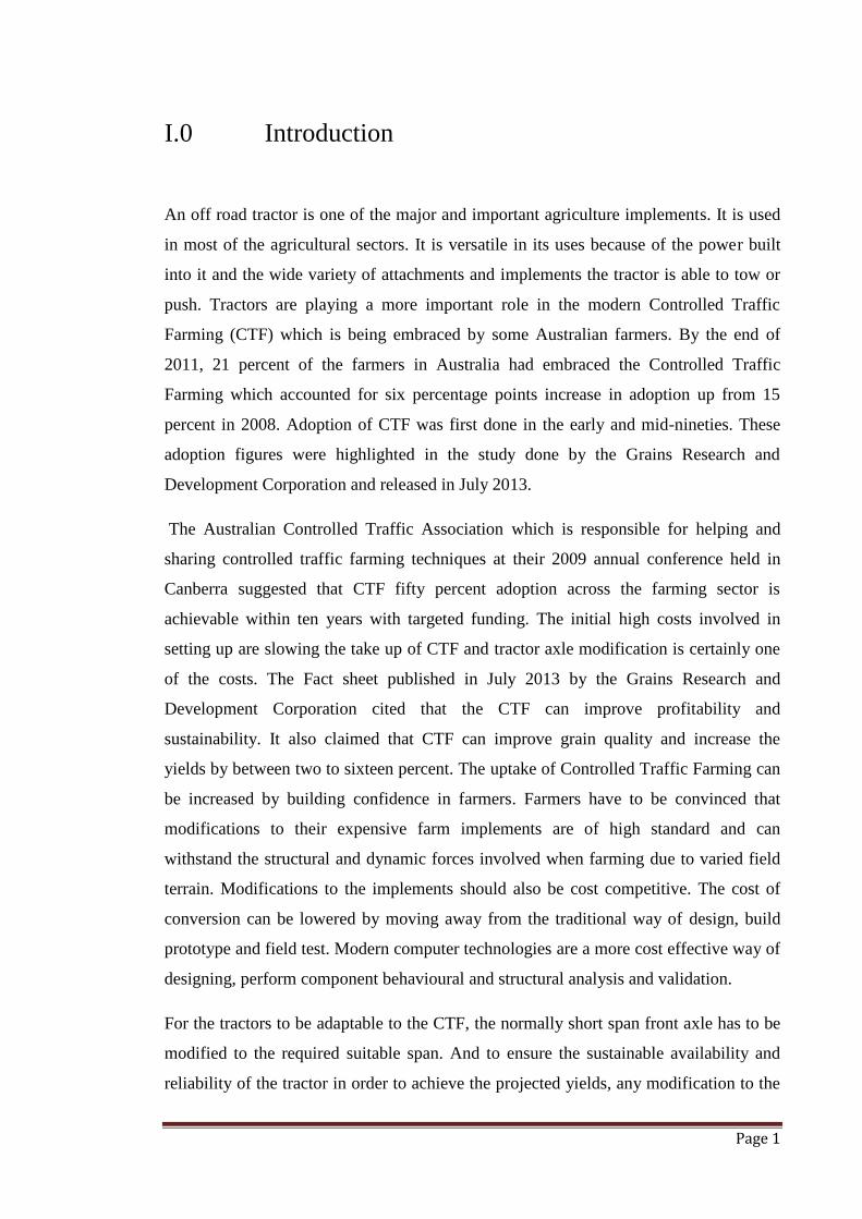
I.0 Introduction
An off road tractor is one of the major and important agriculture implements. It is used
in most of the agricultural sectors. It is versatile in its uses because of the power built
into it and the wide variety of attachments and implements the tractor is able to tow or
push. Tractors are playing a more important role in the modern Controlled Traffic
Farming (CTF) which is being embraced by some Australian farmers. By the end of
2011, 21 percent of the farmers in Australia had embraced the Controlled Traffic
Farming which accounted for six percentage points increase in adoption up from 15
percent in 2008. Adoption of CTF was first done in the early and mid-nineties. These
adoption figures were highlighted in the study done by the Grains Research and
Development Corporation and released in July 2013.
The Australian Controlled Traffic Association which is responsible for helping and
sharing controlled traffic farming techniques at their 2009 annual conference held in
Canberra suggested that CTF fifty percent adoption across the farming sector is
achievable within ten years with targeted funding. The initial high costs involved in
setting up are slowing the take up of CTF and tractor axle modification is certainly one
of the costs. The Fact sheet published in July 2013 by the Grains Research and
Development Corporation cited that the CTF can improve profitability and
sustainability. It also claimed that CTF can improve grain quality and increase the
yields by between two to sixteen percent. The uptake of Controlled Traffic Farming can
be increased by building confidence in farmers. Farmers have to be convinced that
modifications to their expensive farm implements are of high standard and can
withstand the structural and dynamic forces involved when farming due to varied field
terrain. Modifications to the implements should also be cost competitive. The cost of
conversion can be lowered by moving away from the traditional way of design, build
prototype and field test. Modern computer technologies are a more cost effective way of
designing, perform component behavioural and structural analysis and validation.
For the tractors to be adaptable to the CTF, the normally short span front axle has to be
modified to the required suitable span. And to ensure the sustainable availability and
reliability of the tractor in order to achieve the projected yields, any modification to the
Page 2
farm implements including tractors should be done to high standard and in accordance
with relevant standards. This ensures the modifications do not suffer premature failure.
This research project seeks to analyse the structural and dynamic implications on a
modified front axle for a JD 8530 tractors using Finite Element Analysis. Creo 2.0
Simulate will be mainly used for this analysis. This structural and dynamic analysis will
also be done in other available software such ANSYS and Solidworks to compare and
validate the results obtained in Creo 2.0 Simulate with time permitting and if such a
comparison is necessary.
To simulate the changing terrain of the field, the model of the axle will be subjected to
different loading cases and constraints. The Certification load cases as defined for the
project will include drop test, Torture Test, The Impact Test, Pit test, Worst load testing
and one side impact test. These tests are discussed in more detail under section 4.4
Relevant Standards and Certification Tests.
The above mentioned test cases will be used as loading and boundary constraints
conditions for the finite element analysis of the modified tractor front axle. These
testing cases will be used to fulfil the main objective of the project which is to
determine maximum safe loading capacities of the axle. Recommendations including
any further modifications to the axle will be made depending on the outcome of the
comprehensive analyses involving the different loading and constraining conditions.
Outcome of the analyses will also determine whether there is need to create a parametric
model of the axle. A parametric model has critical controlling parameters which can be
altered. Alterations to these controlling parameters ultimately change any dependent
parameters. A parametric model will be crucial if the initial analyses indicate high stress
levels in some components. It is easier and much faster to alter the components
dimension in a parametric model than in a standard 3D model where individual
components geometry has to be edited.

Page 3
2.0 Project Background
Figure 2.1: Controlled traffic farming in practice.
Controlled Traffic Farming (CTF) is an agricultural system that seeks to minimize the
damaging effects of compaction by concentrating wheel traffic to a small area of the
field. This is achieved by bringing the front wheels in line with the rear wheels there
reducing the overall width of the field area that is being affected by the wheels. The
impacted area reduction can be range from 30 to 50 percent depending on the relative
sizes of the wheels. The photo in Figure 2.1 shows a narrow distinctive road that has
been created due to practice of controlled traffic farming. This ensures that the farm
implements use the same tracks all the time. Precision on use of these defined roads
have now been improved by incorporation of Global Positioning Systems into the
farming system. Farm implements including the tractors are modified to suit different
span variations of CTF. Variations in span are 3m, 6m, 9m and 12 metres.
C & C Machining & Engineering, a local engineering company in Toowoomba,
Queensland have been involved with widening a great variety of tractors to enable
farmers to practice the very effective and increasingly popular controlled traffic farming
methods. They claim that they have been modifying the tractors for past 15 years.
Controlled farming has certainly been in practice for considerably long time, two
decades to be precise and major tractor suppliers such as John Deere and Massey
3 metre span road tracksformed by the inlinetractor wheels
Front Axle extended to bringthe front wheels in line with theback wheels.
Page 4
Ferguson have not embraced the growing need of this agricultural changing and
growing market. Controlled farming seeks to separate the field into farm cropping
sections and permanent roads which can be used by all agricultural implements such as
combine harvesters and tractors. Extending the front axle brings the front wheels in line
with the rear wheels and ensures that they are always on the same track thereby creating
some permanent roads on the field. The figure 2.1 above shows the tractor with
extended front axle performing controlled traffic farming.
Precision Agriculture (2011) noted that the common spacing or the span of the wheels is
normally 3metres and there are other spacing variations such as 9m and 12metres. This
effectively means that a 9 and 12 metre span machine can utilise the existing 3 metre
roads if the intermediate spacing matches. They also claimed that CTF farming
improves the agricultural output. Some studies have been done on the impact of
converting to controlled traffic farming on the field yields. Studies carried out by
various researchers including Botta, et al (2007), Braunack (2008) and Jensen and Neale
(2001) cited in Neale, T (2010) showed that yields are reduced by compaction due to
harvest traffic in uncontrolled traffic farming. The yield reductions were considered to
range from 15 percent to 30 percent. This translated to losses to the farmers of between
$150 to $300 per hectare. The cost of adopting or converting to controlled traffic
farming can be recouped within a few years if the losses due to compaction are
eradicated by reducing the area in the field exposed to traffic. This ultimately improves
the yield and the profit margins.
Improvements in paddock of field efficiencies and reduced input costs are realised due
to controlled traffic farming. Other advantages of CTF include reduction in fuel usage
claimed to be in the 50% margins, enables greater accuracy of placing inputs, improves
water infiltration and storage, improves timeliness of operations, and reduces operator
fatigue. A study by Jensen et al (2012) in Denmark on the socio-impacts of controlled
farming in Denmark concluded that the Danish Gross Domestic Product (GDP)
increased by 34 million euros due to the implementation of Precision farming (PF) and
CTF on larger farms in Denmark. The results also clearly showed that adoption of PF
and CTF farming systems will benefit the environment. They were able to verify
reduction of environmentally harmful agricultural inputs such as reduced pesticides and
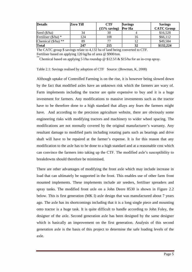
fuel. A case study by Bowman, K (2008) on a group of farms owned by Clifton Allora
Top Crop concluded that there are indeed cost and environmental benefits. The table
shows how the group benefitted by the adoption of controlled traffic farming.
Page 5
Details Zero Till CTF Savings Savings(15% saving) Per Ha CATC Group
Seed ($/ha) 34 30 4 $16,528Fertiliser ($/ha) * 124 108 16 $66,112Chemical ($/ha) ** 89 77 12 $49,584Total 247 215 32 $132,224The CATC group $ savings relate to 4,132 ha of land being converted to CTF.Fertiliser based on applying 120 kg/ha of urea @ $900/ton.**
Chemical based on applying 5 l/ha roundup @ $12.5/l & $15/ha for an in-crop spray.
Table 2.1: Savings realised by adoption of CTF Source: (Bowman, K, 2008)
Although uptake of Controlled Farming is on the rise, it is however being slowed down
by the fact that modified axles have an unknown risk which the farmers are wary of.
Farm implements including the tractor are quite expensive to buy and it is a huge
investment for farmers. Any modifications to massive investments such as the tractor
have to be therefore done to a high standard that allays any fears the farmers might
have. And according to the precision agriculture website, there are obviously some
engineering risks with modifying tractors and machinery to wider wheel spacing. The
modifications are not normally covered by the original manufacturer’s warranty. Any
resultant damage to modified parts including rotating parts such as bearings and drive
shaft will have to be repaired at the farmer’s expense. It is for this reason that any
modification to the axle has to be done to a high standard and at a reasonable cost which
can convince the farmers into taking up the CTF. The modified axle’s susceptibility to
breakdowns should therefore be minimised.
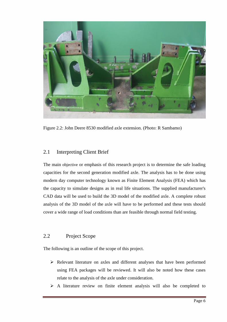
There are other advantages of modifying the front axle which may include increase in
load that can ultimately be supported in the front. This enables use of other farm front
mounted implements. These implements include air seeders, fertiliser spreaders and
spray tanks. The modified front axle on a John Deere 8530 is shown in Figure 2.2
below. This is first generation (MK I) axle design that was manufactured about 7 years
ago. The axle has its shortcomings including that it is a long single piece and mounting
onto tractor is a huge task. It is quite difficult to handle according to John Foley, the
designer of the axle. Second generation axle has been designed by the same designer
which is basically an improvement on the first generation. Analysis of this second
generation axle is the basis of this project to determine the safe loading levels of the
axle.
Page 6
Figure 2.2: John Deere 8530 modified axle extension. (Photo: R Sambamo)
2.1 Interpreting Client Brief
The main objective or emphasis of this research project is to determine the safe loading
capacities for the second generation modified axle. The analysis has to be done using
modern day computer technology known as Finite Element Analysis (FEA) which has
the capacity to simulate designs as in real life situations. The supplied manufacturer's
CAD data will be used to build the 3D model of the modified axle. A complete robust
analysis of the 3D model of the axle will have to be performed and these tests should
cover a wide range of load conditions than are feasible through normal field testing.
2.2 Project Scope
The following is an outline of the scope of this project.
Relevant literature on axles and different analyses that have been performed
using FEA packages will be reviewed. It will also be noted how these cases
relate to the analysis of the axle under consideration.
A literature review on finite element analysis will also be completed to

Page 7
determine the best practices of analysis used in the industry. This will ensure
that best and more reliable results are attained.
Discussion of different loading situations or cases which include:
Drop test, Torture Test, The Impact Test, Pit test, Worst load testing and one
side impact test.
Review of literature related to different loading conditions and testing standards
that might have been used in previous similar studies.
Review modified axle Cad files.
Create the 3D models of the axle components and assembly of the components.
Perform static and structural analysis.
Review the results of the FEA, structural and dynamic analysis.
Recommendations, conclusions and any further work to be undertaken.
Page 8
3.0 Literature Review
The first section of this chapter reviews some literature on various types of finite
element analysis software and their underlying theory. This will seek to establish if
there is any FEA software that is better than the other one. This of course is in relation
to accuracy of the results, ease of use, interface, processing times, computer
requirements and the overall cost of setting up.
The second part will review any available literature on tractor or some other heavy duty
both on field and off field vehicle axle analysis. This review will give an insight into
how other analyses have been done and any flaws in the reports. These will also enable
to evaluate the benchmarks against which the tests were performed and any relevant
engineering standards applied. Different types of axles will also be reviewed.
3.1 Finite Element Analysis
Finite element analysis (FEA) is defined as a numerical method of solving engineering
problems that would otherwise be difficult to solve using analytical methods. Its main
uses are quite varied and include calculation of stresses, deflections and displacements
in both simple and complex structures. The application of FEA has also been extended
to thermal, structural and fluid flow analysis. Despite its application to many different
engineering fields the underlying theory is the same.
The structure or component under analysis is basically divided into sections which are
more manageable and easy to manipulate. This process is called discretization and
according to Logan, the finite element method involves modelling the structure using
small interconnected elements called finite elements and a displacement function is
associated with each finite element. These elements are then linked either directly or
indirectly, to every other element through common or shared interfaces, including nodes
and/or boundary lines and/or surfaces. The material’s known stress and strain properties
making up the structure are then used to determine the behaviour of a given node in
terms of the properties of every other element in the structure. These are formulated into
equations for every node and the total set of equations obtained can be solved using
matrices to get the overall behaviour in the structure. Matrices are easier to evaluate
than the complicated differential equations which result from analytical analysis. The
Page 9
numerical method gives an estimate result which can be improved by increasing the
number of nodes and this obviously results in an even larger set of equations.
Computational power of the computer can be utilised to solve these sorts of equations
and that is the underlying theory of the FEA software.
3.1.1 Why use Finite Element Analysis
1. It is used as a cost effective way of verifying that a new design or a
modification to an existing structure or component will meet the required
structural, modal or thermal specifications. The traditional way of manufacturing
which involves designing, building a prototype and field testing is expensive
because the structural behaviour is not known until the new design has been
subjected to field testing. Any subsequent problems that may arise with the new
design would mean the prototype will have to be redesigned and modified at a
cost. Use of Finite Element Analysis removes the need to build a prototype for
testing purposes. The new model is tested and modified accordingly before the
component is manufactured or fabricated. FEA analysis is effectively a cost
cutting exercise. Behaviour of a component is determined before manufacture
and saves on building a prototype which may not be able to meet the
specifications.
2. The component or components are loaded and constrained as in real situation.
Finite element analysis allows loads simulating the real situation to be applied to
the model. Constraints such as displacements, planar and pin can also be applied
to mimic actual situations where components can be fixed in various translations
or may be joined used a pin joint which allows rotation.
3. The results as to how the component will behave under the suggested loadings
and constraints can be processed within short time depending on the complexity
of the component and the computer capabilities. A model’s geometry can be
easily altered if the results of an analysis are not satisfactory.
4. The results outcomes from a finite element analysis can be relied on. This
depends on the skill level of the analyst. Proper application of the software
can produce results that are quite reasonable. León, O, N, Martínez, P, Orta C, P,
Adaya (2000) did an experiment to verify the validity of results obtained from a
finite element analysis. They concluded that the results of the experiment had a
Page 10
5.17% variation from the finite element analysis results. The challenge though is
in the interpretation of the FEA results provided that the loadings and constraints
have been appropriately applied to a well prepared model. According to Toogood,
R, (2012) the results obtained from an FEA modelling depends on the quality of
the input data. He says the principles of garbage in garbage out (GIGO) apply
when using an FEA package. Results could be improved by either adjusting the
model’s meshing or redefining the convergence of the result. The number of
elements and nodes in the model can be increased by changing the convergence of
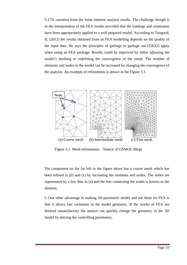
the analysis. An example of refinements is shown in the Figure 3.1.
(a)-Course mesh (b)-Intermediate mesh (c)-Fine mesh
Figure 3.1: Mesh refinements. Source: (COSMOL Blog)
The component on the far left in the figure above has a coarse mesh which has
been refined in (b) and (c) by increasing the elements and nodes. The nodes are
represented by a few dots in (a) and the line connecting the nodes is known as the
element.
5. One other advantage in making 3D parametric model and use them for FEA is
that it allows fast variations in the model geometry. If the results of FEA are
deemed unsatisfactory the analyst can quickly change the geometry in the 3D
model by altering the controlling parameters.
Node

Page 11
3.1.2 Types of FEA software
There is a wide variety of FEA packages on the market and they also vary in their
capabilities, pricing and ease of use. A list of FEA packages is shown in Appendix
12. There are 68 FEA software packages that have been compared in the list. They
have been compared mainly on their pricing, capabilities, ability to import CAD
drawings and types of elements that can be handled. Some of the free software are
limited in their capabilities for example FELIPE is only capable of performing
four functionalities out of a possible twenty three. There are packages that have
extensive capabilities despite being freeware. A package like Elmer is capable of
performing around 15 functions out of the possible twenty three. The fact that a
package is paid software does not necessarily give it more capabilities than some
of the freeware.
Packages are designed for specific applications and it is the ability to perform that
particular application that should be considered when deciding which FEA
package to use. The applications include the static and structural analysis,
Thermal, Computational Fluid dynamics and many more. It is no uncommon to
find high cost packages that are quite limited in their applications. These are
designed for special applications such as in fluid flow analysis and civil and
structural designs. The industry most common packages with a lot of capabilities
are ADINA, ANSYS Mechanical NEi/Nastran, Pro/MECHANICA Wildfire 2,
COSMOSWorks, COMSOL and Strand 7.
3.1.3 FEA software results comparison
Literature sought on comparison of results from different Finite Element Analysis
suggests that if the same model is analysed under different platform, the results
should be approximately the same. The results would be the same or close if the
loads and constraints are applied correctly in each platform used. Adams, V of
Impact Engineering Solutions did an experiment to check if the results of an FEA
on different platforms were the same. In the experiment four widely used
packages were used namely COSMOSWorks Version 2005, ANSYS Version 8.1,
NEi/Nastran Version 8.3 and Pro/MECHANICA Wildfire 2. Some of the results
from the comparison are shown in Table 3.1 below.

Page 12
Table 3.1: Comparison of FEA software results Source: (Adams, V)
It was concluded that the results had variations of up to 10% and thus the results from
all platforms were reasonably consistent.
3.2 FEA Validation and Verification
The discussion in the above section revolved around how use of different FEA platform
influenced the results but the big question is how those results compare to the actual
experimental results. The FEA results have to be validated to build some confidence in
the outcomes of FEA analysis. An experiment was carried out by Koyuncu, A, Gökler,
M, Balkan, T, (2011) to verify the results of FEA on a front axle support for a tractor.
Strain gauges were placed on the axle support to measure and calculate the stress under
the same loading condition as in the FE Analysis. Results of the experiment were found
to have a variance of 7.7% form the FEA results. This basically confirmed that the FEA
results can be relied on. MSC/Nastran and Patran finite element analysis packages were
used to perform an analysis on the axle support.
Another experiment by N. León, O, Martínez, P, Orta C, P. Adaya, 2000 on front axle
beam of a truck sought to validate the results of an FE Analysis. MSC Patran/MSC
Nastran V. 8 was used to perform the finite element analysis. PhotoStressO which they
claim to be a widely used technique for accurately measuring surface strains was used to
Page 13
measure the stress. They found some that the results of the experiment and the finite
element analysis were close and there was a variation of 5.17% in the overall results.
It can therefore be safely concluded that Finite Element Analysis is a reliable and a cost
effective way of checking the integrity of designs or modifications. The FEA results
correlates favourably with the experimental outcomes. Any platform or the type of
software used for an analysis as long as it has the necessary capabilities to perform the
particular analysis and the user is competent in its use. Creo 2.0 Parametric and Creo
2.0 Simulate were chosen for the analysis of the modified axle in this project. Creo 2.0
Parametric was used to create the 3D models of the axle components and the complete
or assembled model of the axle. The Simulation arm of Creo 2.0 was then used for the
finite element analysis of the model. Creo 2.0 Parametric and Simulate although not as
popular as the other packages previously discussed was chosen for this project because
of its capabilities to perform the required static structural analysis of the modified axle.
Other reasons for selecting this particular package include costs and user competency.
The package was already on my computer because it had been used in previous courses
such computational mechanics so there was no cost involved.
3.3 Tractor front axle designs and modifications
Literature on FEA analysis on tractor axle designs and modifications available is not
very extensive and this most probably because of business and property protection
issues. The few that are available mainly deal with optimisation of axle designs. An
optimisation study was done by Mahanty, D et al and mainly designed an axle with the
aim of reducing the weight of the current designs. They managed to reduce the weight
of the axle while maintaining the structural and dynamic integrity. ANSYS software
was used in this particular analysis and the new designs with reduced weight showed
some 15% increase in stresses and displacements which was deemed significantly low.
They also managed to reduce the weight by 40 %. This study shows that FEA can be a
very effective tool in design and component modification which can ultimately cut
costs. 40% reduction is quite significant and depending on the production quantities the
savings can also be huge.
León, N (2000) seems to confirm the theory that costs are really reduced by optimising
axle design through implementing FEA. In their study they managed to validate and
Page 14
back the results from the FEA analysis by performing series of experimental test. In
their research León, N concluded that the proposed engineering development process at
their DIRONA site proved to be useful in reducing the development time and costs,
while maintaining highest product quality and reliability. The software used in this
study is SC Patran / MSC Nastran V. 8.0 was used. The axle design or modification can
be improved by changing the variables or parameter which includes the materials and
the component dimensions which show high levels of stress and strain. Changing some
features such as the holes, undercut, radius and their location on a component can also
improve the general stress and displacement results. León, N managed to reduce the
weight of the axle by 6.8% by changing the design parameters. The stress only
increased by 2% which is negligible. According to Aloni, S, Khedkar, S in their
comparative analysis of an axle, they also managed to reduce the weight by 10 percent
by changing the material from Steel SAE 1020 – Hot Rolled to ASTM A536 (65-45-12)
Ductile Iron – Castings. Factor of Safety was improved from 0.7 to 2.4. From these
studies it can concluded that modifications and optimisation can be done without
compromising the integrity of the component.
Up to this point the literature reviewed did not include the effects of the dynamic forces
which are considered significant at high speed. In addition to normal reaction forces on
the axle due to the rugged terrain of the field, dynamic forces also have to be considered
in the analysis of the behaviour of the axle. Koyuncu, A, Gökler, M, Balkan, T, (2011)
outlined the importance of this dynamic feature of the analysis and put it as equivalent
to 3g force. The loadings due to dynamic forces are discussed in detail under section
4.4.
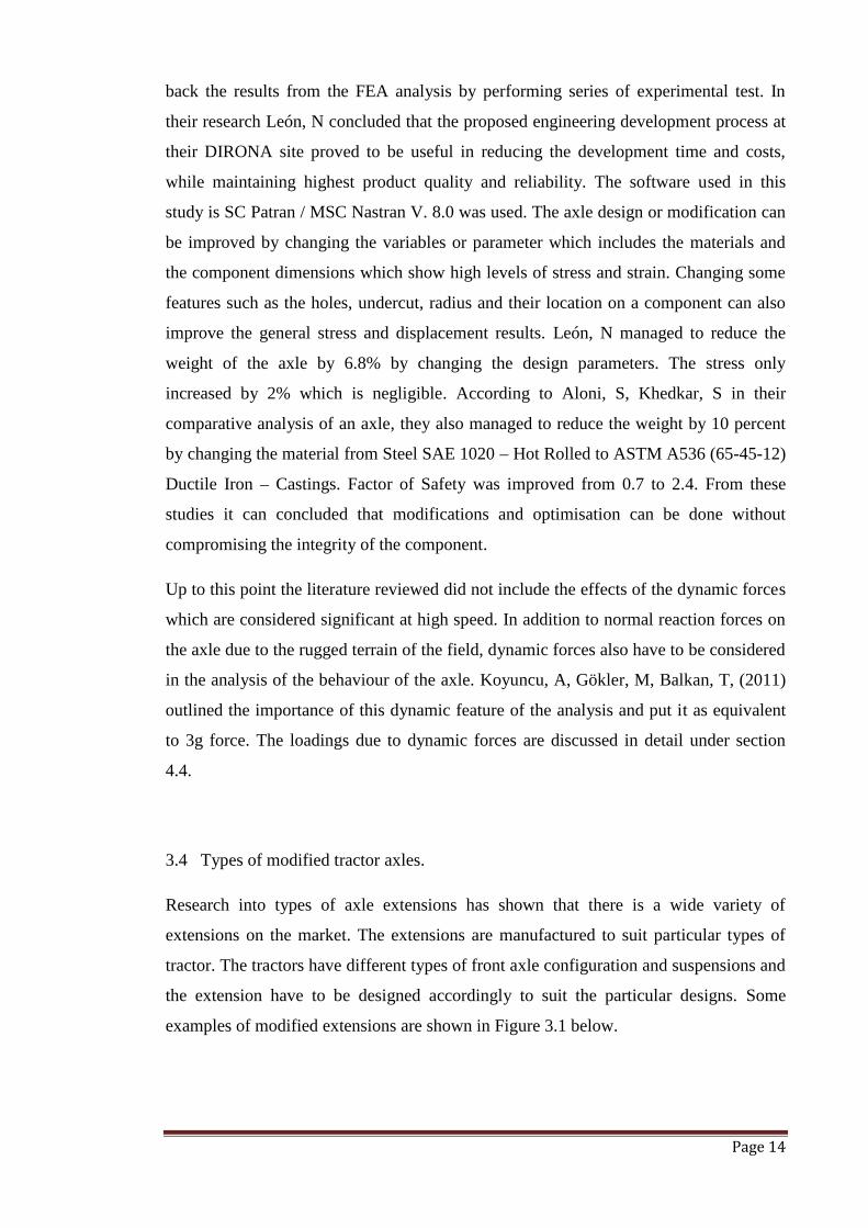
3.4 Types of modified tractor axles.
Research into types of axle extensions has shown that there is a wide variety of
extensions on the market. The extensions are manufactured to suit particular types of
tractor. The tractors have different types of front axle configuration and suspensions and
the extension have to be designed accordingly to suit the particular designs. Some
examples of modified extensions are shown in Figure 3.1 below.
Page 15
Figure 3.1: John Deere round bail cotton picker extension. (Source: C and C Machining)
In the left photo of Figure 3.1, the original axle enclosed in the blue box has been
moved out to accommodate the extension on the left. The axle is a bit complicated than
the one shown in the right photo. A provision for the steering rod in the extension
creates some manufacturing challenges. Both axles shown in Figure 3.2 result in large
moment arms which ultimately put high level stress on the parts joined to the tractor
axle or the mounting parts on the wheel end. C and C Machining on their website stated
that tubular sections have proved to increase stress on the kingpins on the front axle
which may ultimately leads to failure.
Tractors are a huge investment for farmers costing several hundred hundreds of
thousands of dollars and conversion costs to controlled traffic farming which may be
prohibitive, breakdowns resulting in downtime and added costs is the least of things the
farmers have to worry about. This affects the uptake of controlled traffic farming by the
farmers for this creates uncertainties around the performance of the modified axle
extensions. The traditional method of building a prototype and performing field tests to
measure the performance and structural integrity of a design is becoming outdated and
it’s not something the farmers want to rely on. Analysis of modified extensions using
the now powerful FEA software that has been tested and results validated over the years
could boost the confidence of farmers on these modifications. The older tractors without
front suspension had to be equipped with a tubular section due to the configuration of
the driver train and the suspension. More types of axle extensions are shown below.
Original axle
Axle extension
Steering Rod
Tubular axleextensions
Page 16
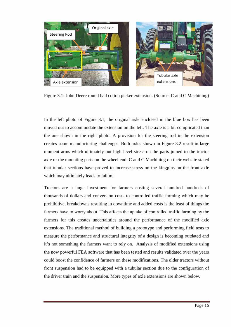
Figure 3.2: Axle extensions. Source: Larocque, S, 2012 Nuffield Report.
These tractor types shown above do not have a front wheel suspension such as the one
incorporated into the JD8530 which enables the front wheels to move up and down in
response to the terrain while maintaining the whole tractor level and stable. Detailed
discussion of the JD8530 modified axle is in the next chapter.
Axle extensionAxle extension
Page 17
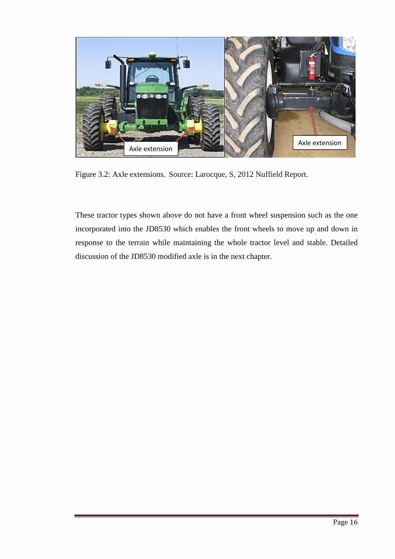
4.0 Tractor Specifications
John Deere 8530 tractor was manufactured out of United States of America by one of
the biggest tractor manufacturers John Deere. It was manufactured from 2006 to 2009.
Figure 4.1: JD8530 tractor. Source (Chris Snook)
Tractor Information or data is in Appendix D. The tractor cost around AU$200 000 to
buy second hand and is a huge investment for farmers. Any modification to such
equipment has to be of very high standard. The modifications to the front axle of this
tractor were complex because of the independent front suspension rams, drive line and
the steering rod all of which had to be considered in the axle design. And because of the
incorporation of the independent suspension, the tractor is capable of high speeds
reaching up to 50 km/h without compromising the comfort of the ride.
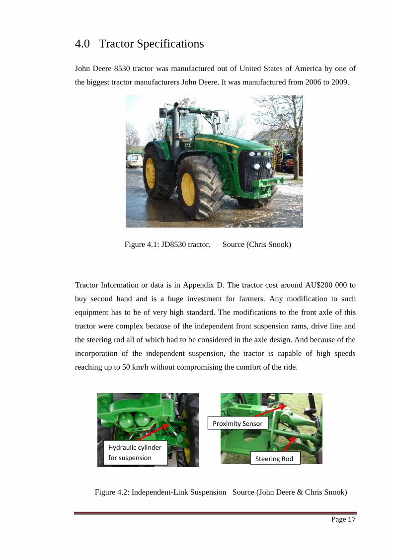
Figure 4.2: Independent-Link Suspension Source (John Deere & Chris Snook)
Hydraulic cylinderfor suspension
Proximity Sensor
Steering Rod

Page 18
The proximity sensor indicated in Figure 4.2 senses the position in space of pin coupled
to the top wishbone and communicates to the control unit which ultimately adjust the
wishbones up or down through the hydraulic ram thereby maintaining the level of the
tractor. Modifications to the front axle should not compromise such functionalities and
its accessories.
4.1 General dimensions and weight.
The Figure 4.3 below shows the overall dimensions of the tractor and the measure that
was worth taking note was the operating weight of the tractor. This measure was used in
the determination of loads on the tractor axle.
Operating Weight 12156 kg
Wheelbase (D) 3020 mm
Length (A) 5560 mm
Height (C) 3120 mm
Figure 4.3: Tractor dimension and weight Source (Tractordata.com)
Page 19
4.2 Original front axle configuration
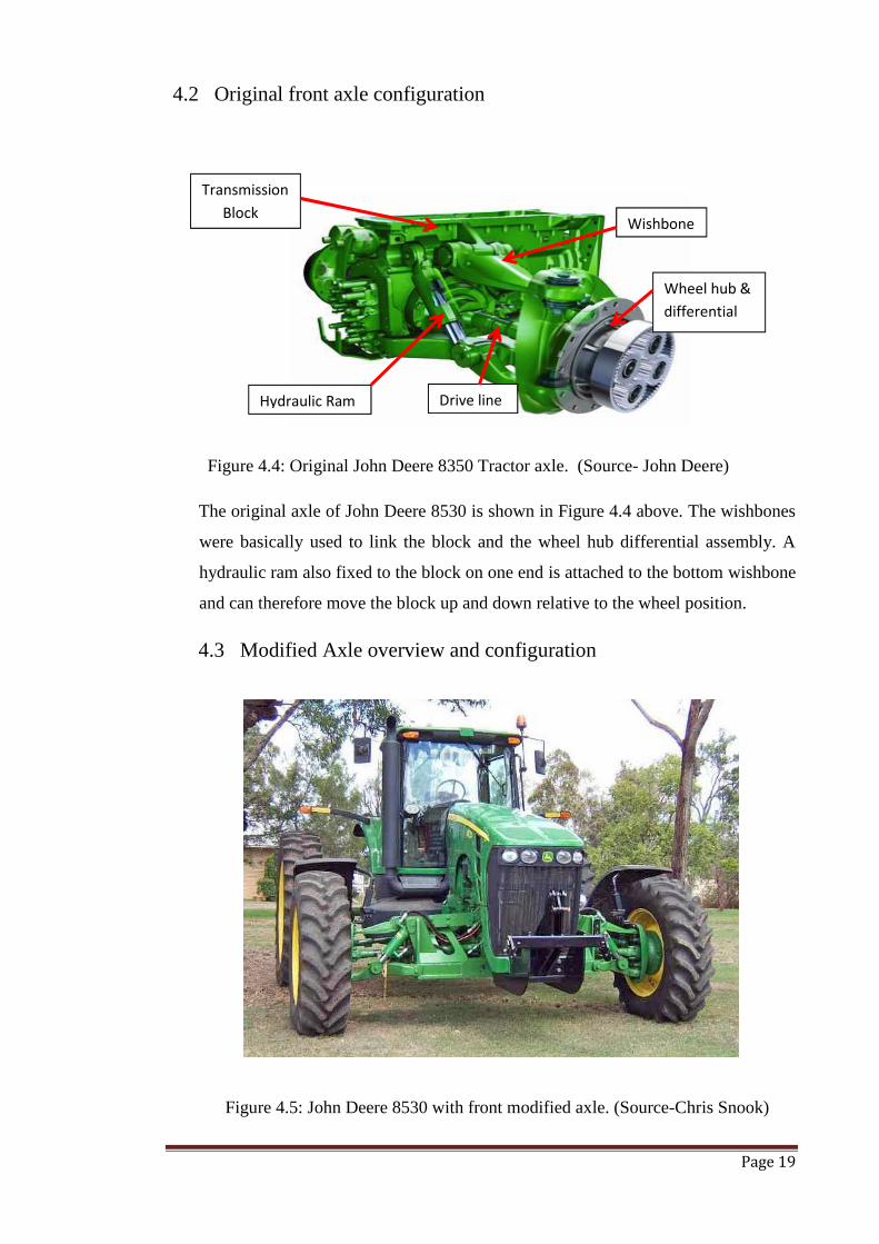
Figure 4.4: Original John Deere 8350 Tractor axle. (Source- John Deere)
The original axle of John Deere 8530 is shown in Figure 4.4 above. The wishbones
were basically used to link the block and the wheel hub differential assembly. A
hydraulic ram also fixed to the block on one end is attached to the bottom wishbone
and can therefore move the block up and down relative to the wheel position.
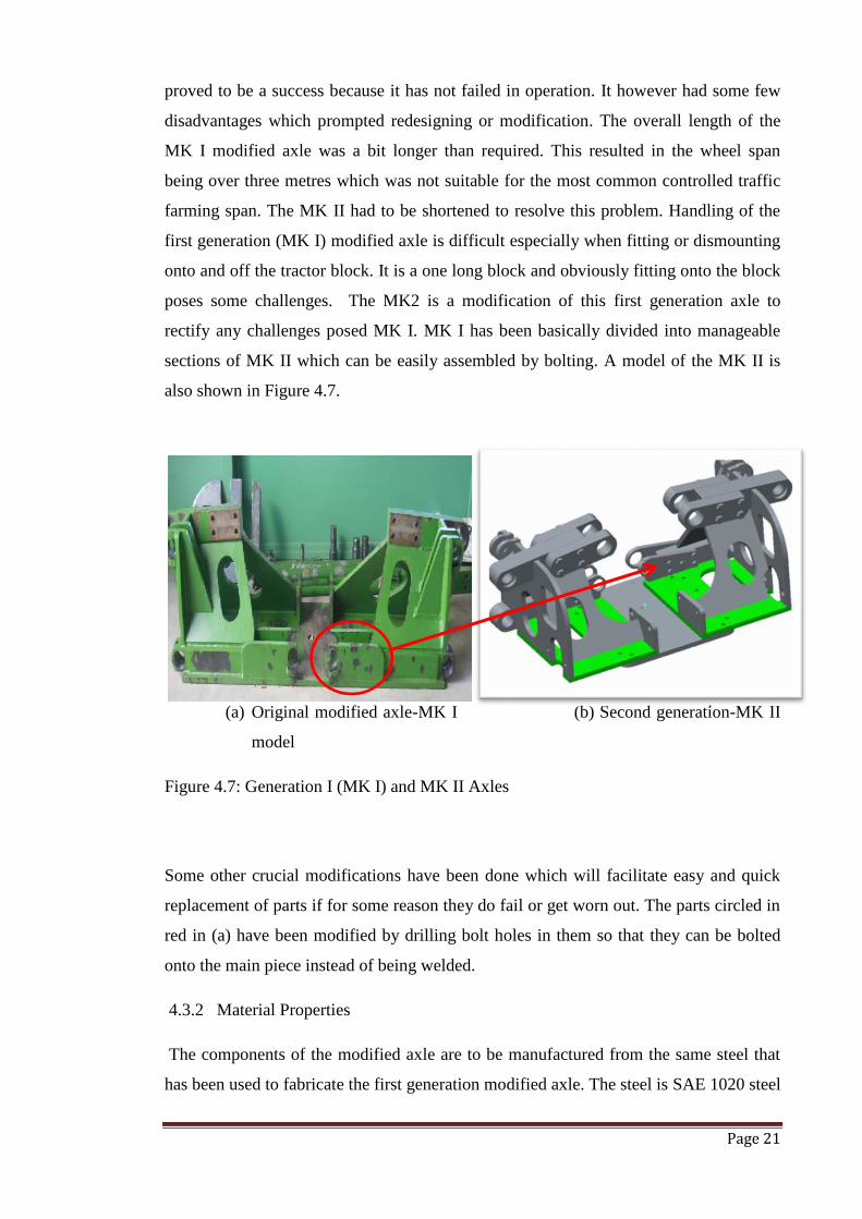
4.3 Modified Axle overview and configuration
Figure 4.5: John Deere 8530 with front modified axle. (Source-Chris Snook)
Hydraulic Ram
Wishbones
Drive line
TransmissionBlock
Wheel hub &differential

Page 20
Figure 4.6: Modified John Deere 8350 Tractor axle at close range.
The modified axle is basically a welded and bolted steel block that has been inserted in
between the tractor gearbox or transmission block and the wishbones as shown in the
figure above. This increases the wheel span of the front axle and increases the
performance of the tractor, The new axle is attached to the block using the existing
anchor points to which the wishbones were previously attached. The wishbones were
moved further out to the new anchoring points on the new axle while still connected to
the old existing ones on the wheel side. The axle component parts are discussed in more
detail in section 5.
4.3.1 Difference between the two (MK I) and MK II Axles designs
The first generation axle which will be referred to as MK I design in the report is the
shown on the left side in Figure 4.7 below has been in use for past seven years. It has
Original Wishbones
Suspension Ram
First GenerationModified Axle
TransmissionBlock
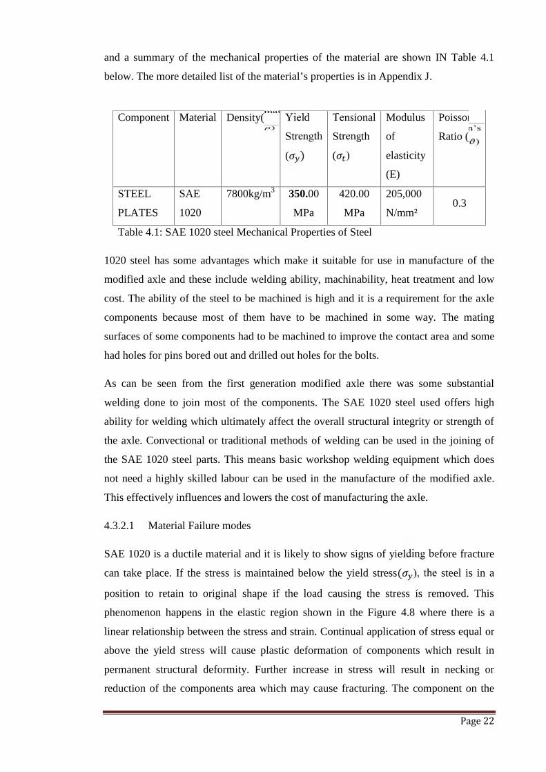
Page 21
proved to be a success because it has not failed in operation. It however had some few
disadvantages which prompted redesigning or modification. The overall length of the
MK I modified axle was a bit longer than required. This resulted in the wheel span
being over three metres which was not suitable for the most common controlled traffic
farming span. The MK II had to be shortened to resolve this problem. Handling of the
first generation (MK I) modified axle is difficult especially when fitting or dismounting
onto and off the tractor block. It is a one long block and obviously fitting onto the block
poses some challenges. The MK2 is a modification of this first generation axle to
rectify any challenges posed MK I. MK I has been basically divided into manageable
sections of MK II which can be easily assembled by bolting. A model of the MK II is
also shown in Figure 4.7.
(a) Original modified axle-MK I (b) Second generation-MK II
model
Figure 4.7: Generation I (MK I) and MK II Axles
Some other crucial modifications have been done which will facilitate easy and quick
replacement of parts if for some reason they do fail or get worn out. The parts circled in
red in (a) have been modified by drilling bolt holes in them so that they can be bolted
onto the main piece instead of being welded.
4.3.2 Material Properties
The components of the modified axle are to be manufactured from the same steel that
has been used to fabricate the first generation modified axle. The steel is SAE 1020 steel
Page 22
and a summary of the mechanical properties of the material are shown IN Table 4.1
below. The more detailed list of the material’s properties is in Appendix J.
Table 4.1: SAE 1020 steel Mechanical Properties of Steel
1020 steel has some advantages which make it suitable for use in manufacture of the
modified axle and these include welding ability, machinability, heat treatment and low
cost. The ability of the steel to be machined is high and it is a requirement for the axle
components because most of them have to be machined in some way. The mating
surfaces of some components had to be machined to improve the contact area and some
had holes for pins bored out and drilled out holes for the bolts.
As can be seen from the first generation modified axle there was some substantial
welding done to join most of the components. The SAE 1020 steel used offers high
ability for welding which ultimately affect the overall structural integrity or strength of
the axle. Convectional or traditional methods of welding can be used in the joining of
the SAE 1020 steel parts. This means basic workshop welding equipment which does
not need a highly skilled labour can be used in the manufacture of the modified axle.
This effectively influences and lowers the cost of manufacturing the axle.
4.3.2.1 Material Failure modes
SAE 1020 is a ductile material and it is likely to show signs of yielding before fracture
can take place. If the stress is maintained below the yield stress( ), the steel is in a
position to retain to original shape if the load causing the stress is removed. This
phenomenon happens in the elastic region shown in the Figure 4.8 where there is a
linear relationship between the stress and strain. Continual application of stress equal or
above the yield stress will cause plastic deformation of components which result in
permanent structural deformity. Further increase in stress will result in necking or
reduction of the components area which may cause fracturing. The component on the
Component Material Density( ) Yield
Strength
( )Tensional
Strength
( )
Modulus
of
elasticity
(E)
Poisson’s
Ratio ( )
STEEL
PLATES
SAE
1020
7800kg/m3 350.00
MPa
420.00
MPa
205,000
N/mm²0.3
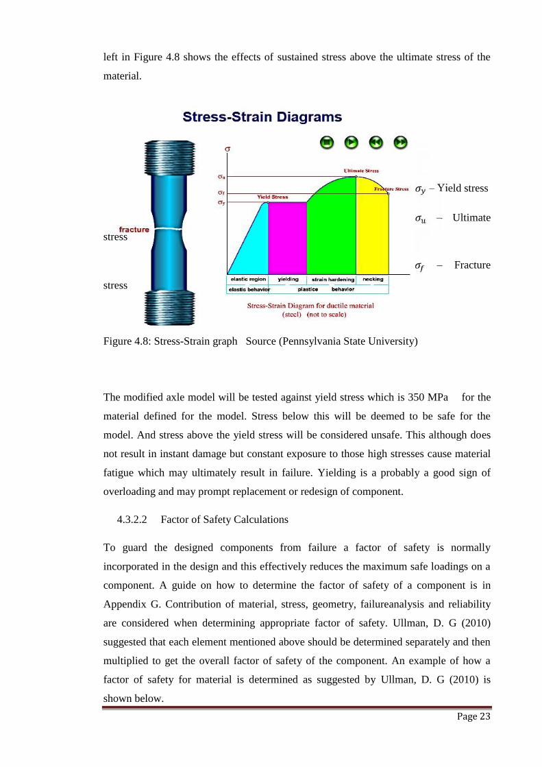
Page 23
left in Figure 4.8 shows the effects of sustained stress above the ultimate stress of the
material.
– Yield stress
– Ultimate
stress
– Fracture
stress
Figure 4.8: Stress-Strain graph Source (Pennsylvania State University)
The modified axle model will be tested against yield stress which is 350 MPa for the
material defined for the model. Stress below this will be deemed to be safe for the
model. And stress above the yield stress will be considered unsafe. This although does
not result in instant damage but constant exposure to those high stresses cause material
fatigue which may ultimately result in failure. Yielding is a probably a good sign of
overloading and may prompt replacement or redesign of component.
4.3.2.2 Factor of Safety Calculations
To guard the designed components from failure a factor of safety is normally
incorporated in the design and this effectively reduces the maximum safe loadings on a
component. A guide on how to determine the factor of safety of a component is in
Appendix G. Contribution of material, stress, geometry, failureanalysis and reliability
are considered when determining appropriate factor of safety. Ullman, D. G (2010)
suggested that each element mentioned above should be determined separately and then
multiplied to get the overall factor of safety of the component. An example of how a
factor of safety for material is determined as suggested by Ullman, D. G (2010) is
shown below.
Page 24
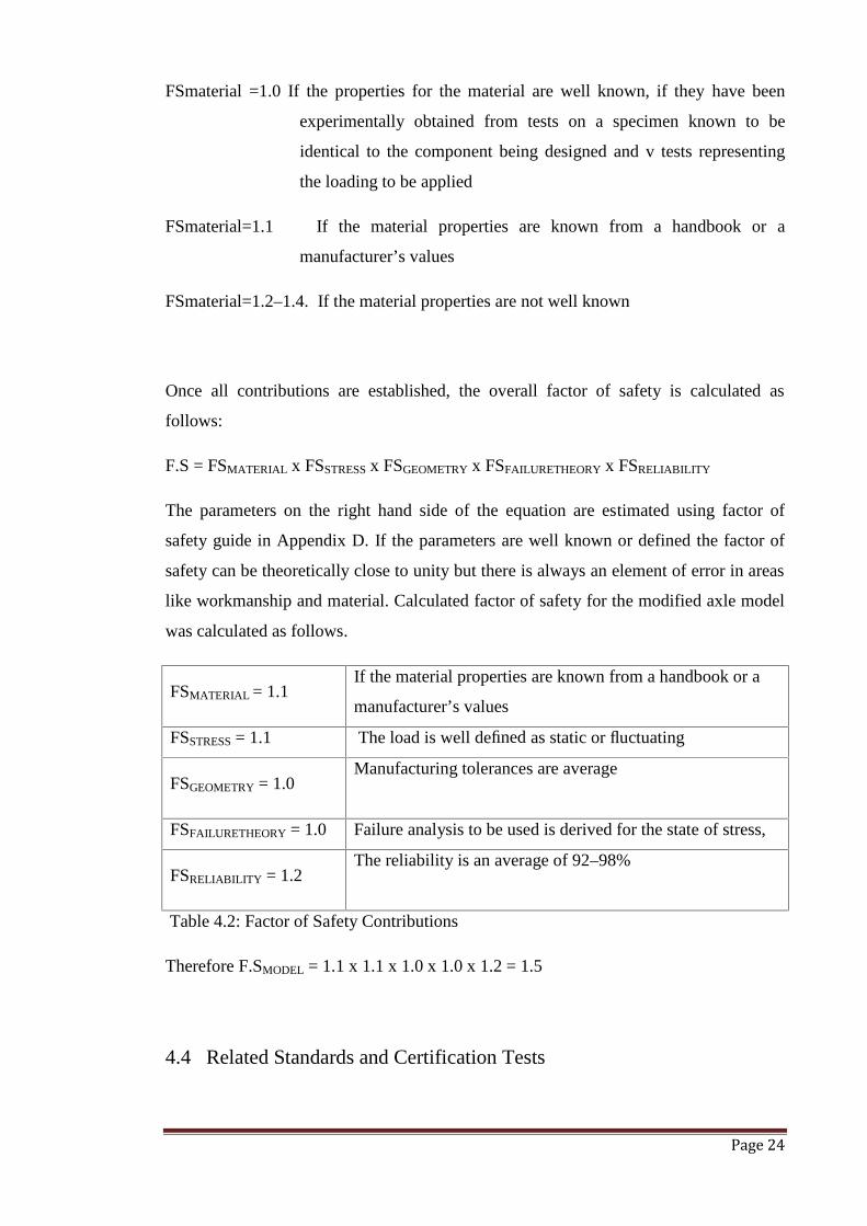
FSmaterial =1.0 If the properties for the material are well known, if they have been
experimentally obtained from tests on a specimen known to be
identical to the component being designed and v tests representing
the loading to be applied
FSmaterial=1.1 If the material properties are known from a handbook or a
manufacturer’s values
FSmaterial=1.2–1.4. If the material properties are not well known
Once all contributions are established, the overall factor of safety is calculated as
follows:
F.S = FSMATERIAL x FSSTRESS x FSGEOMETRY x FSFAILURETHEORY x FSRELIABILITY
The parameters on the right hand side of the equation are estimated using factor of
safety guide in Appendix D. If the parameters are well known or defined the factor of
safety can be theoretically close to unity but there is always an element of error in areas
like workmanship and material. Calculated factor of safety for the modified axle model
was calculated as follows.
FSMATERIAL = 1.1If the material properties are known from a handbook or a
manufacturer’s values
FSSTRESS = 1.1 The load is well defined as static or fluctuating
FSGEOMETRY = 1.0Manufacturing tolerances are average
FSFAILURETHEORY = 1.0 Failure analysis to be used is derived for the state of stress,
FSRELIABILITY = 1.2The reliability is an average of 92–98%
Table 4.2: Factor of Safety Contributions
Therefore F.SMODEL = 1.1 x 1.1 x 1.0 x 1.0 x 1.2 = 1.5
4.4 Related Standards and Certification Tests
Page 25
A search for specific standards governing the design and testing of tractor axle did not
yield results. John Foley, the designer and manufacturer of the JD 8530 front axle
extension confirmed that no industry related standards were being used or referred to.
Previous studies by Mahanty, D, K Manohar, V, Khomane, B, S, Nayak (2002) on the
structural and dynamic analysis of a tractor’s Front Axle however used some test
conditions which they called certification tests. Drop test is one of the certification tests
and is discussed in more detail under section 4.4.1. A crucial assumption that has been
made to facilitate the analysis of the modified axle is that the reactions of the ground to
the wheels are acting directly to the axle. The effects of the suspension and the
wishbones are beyond the scope of this analysis.
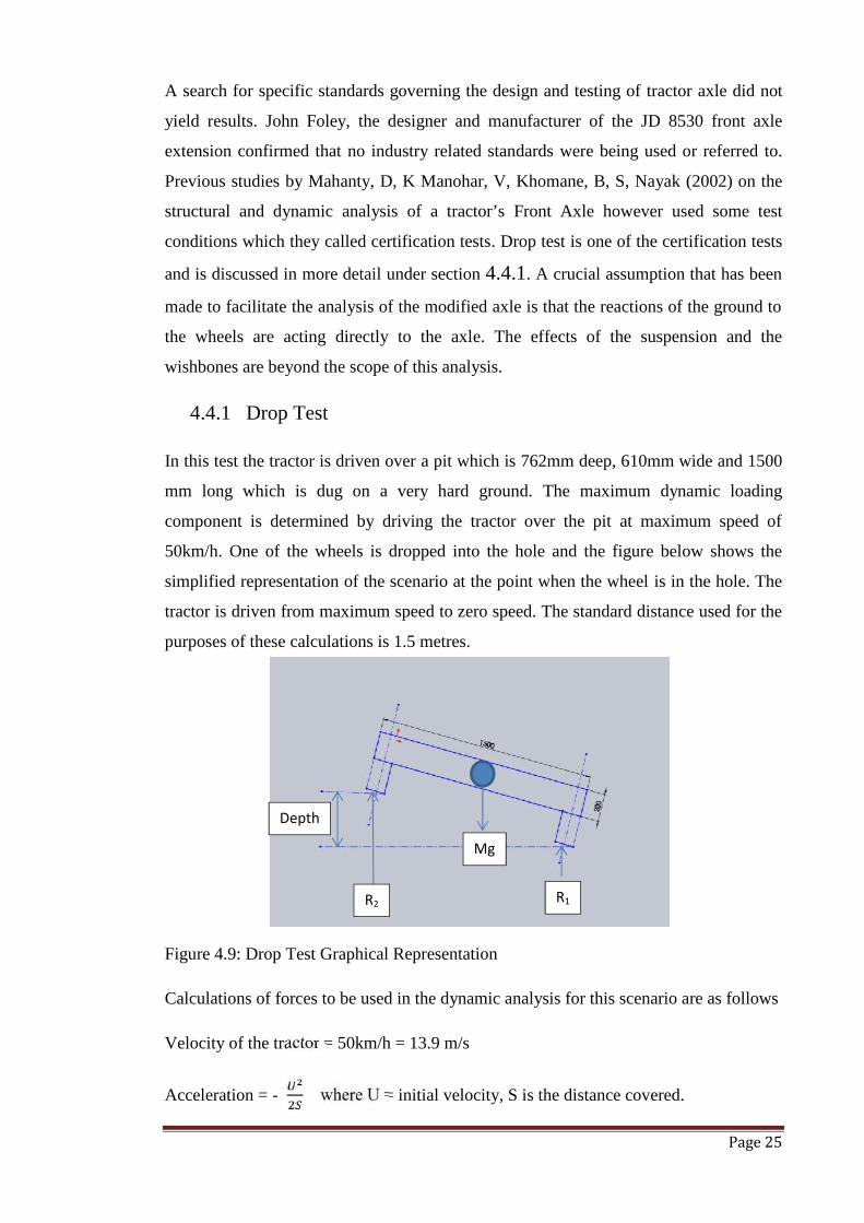
4.4.1 Drop Test
In this test the tractor is driven over a pit which is 762mm deep, 610mm wide and 1500
mm long which is dug on a very hard ground. The maximum dynamic loading
component is determined by driving the tractor over the pit at maximum speed of
50km/h. One of the wheels is dropped into the hole and the figure below shows the
simplified representation of the scenario at the point when the wheel is in the hole. The
tractor is driven from maximum speed to zero speed. The standard distance used for the
purposes of these calculations is 1.5 metres.
Figure 4.9: Drop Test Graphical Representation
Calculations of forces to be used in the dynamic analysis for this scenario are as follows
Velocity of the tractor = 50km/h = 13.9 m/s
Acceleration = - where U = initial velocity, S is the distance covered.
Mg
R2 R1
Depth
Page 26
= -. . = - 64.4 m/s
Using F = mass x acceleration
= 631kg x 64.4 m/s
= 40.687 kN force on the front of the axle due to velocity of tractor.
Mass on the front axle is 45% of the total weight of the tractor of 12000 kg = 5400kg.
Reactions R1and R2 are equal = (5400/2 x 9.81) = 26.487 kN
The other certification tests which include Torture Test, ‘8’ shaped track test, impact
test, pit test and worst load test follow a similar setup as the drop test described above.
The difference is in the scenarios which include differing velocity applied and
orientation of the axle relative to the field.
4.4.2 VSB 14 Tests
Other studies though have used a different approach to the one adopted by Mahanty, D,
K Manohar, V, Khomane, B, S, Nayak (2002) described above. Koyuncu, A & Gökler,
M, I & Balkan, T, (2010) in their strength and fatigue analysis for agricultural tractors,
they simply used 3g and 2g loading cases to simulate the dynamic loads induced by
rugged terrain of the field. VSB14 loading cases used by Krank Engineering are similar
to the ones used by Koyuncu, A & Gökler, M, I & Balkan, T, 2010. These are however
more detailed and there is some loading cases similarity with those used by Mahanty, D,
K Manohar, V, Khomane, B, S, Nayak (2002). Brett Longhurst in his analysis of the
front axle of A Holden also used the VBS 14 loading cases. They basically used three
loading cases which are specified in Vehicle Standards Bulletin 14, a bulletin produced
by department of infrastructure and regional development. The cases though cover
vehicles covered by legislation and off road vehicles are not covered in Australian
government legislation that is according to the department website. The three loading
cases were classified as follows:
1. Loading Case 1: Normal Reaction Loads
Normal weight reaction loads are applied to the ends of the model to simulate
the normal static situation. Governing mode of failure in this analysis is by
yielding.
Page 27
2. Loading Case 2: Bump loads: 4g vertical
This simulates the scenario where the vehicle has to drive over a pothole. This
test is similar to the drop loading case used by Mahanty, D, K Manohar, V,
Khomane, B, S, Nayak (2002) except that the force in this particular case is
already defined as 4g vertical. In addition to the calculated reactional forces on
the axle due to the weight of the vehicle a vertical force equivalent to four times
the weight of the axle also acts in the same direction as the reaction forces. The
additional 4g force is applied to one end of the axle. In this loading case the
materials ultimate tensile strength is used as the upper limit for this test on the
assumption that the critical parameter in this particular test is fracture. The axle
in this analysis is allowed to deform due to yielding but not exceeding the
fracture limits.
3. Loading Case 3: Overturning loads: 2g vertical with 2.5g side load
Overturning can result in some substantial dynamic loads being imposed on the
axle and to simulate such loads the code recommends that 2g vertical and 2.5g
side or lateral loads be applied. The governing failure mode in this analysis is by
yielding.
4. Loading Case 4: Skid loads: 2g vertical with 1.2g longitudinal
Skid loads or braking loads are applied as combined loadings of 2g vertical with
1.2g longitudinal.
5. Loading Case 5: Worst Case Loading
The highest loads in the above four tests are identified for all directions to create
a worst case scenario. These are applied that vertical, lateral and horizontally.
The VSB14 tests were adopted for the analysis of the modified axle because the tests
give higher testing loads. The model is exposed to worst case scenarios in these tests.
These tests are also covered by legislation and this gives some credibility to the tests.
They have been formulated based on wide ranging studies. The certification tests have
not been used anywhere else except by Mahanty, D, K Manohar, V, Khomane, B, S,
Nayak (2002). The VSB14 detailed loading cases are under section 7.1.7.

Page 28
5.0 Review of the e-drawings of the modified axle
The client provided an e drawing of the modified axle. The drawings were initially
drawn in AutoCAD. E drawings can be viewed using e drawings model viewer in
Solidworks and measurements of the components can easily be determined from the
drawing using the measure tool in the software. The Figure below shows the some
drawings of the component as supplied displayed in the Solidworks e-Drawing Viewer.
The drawings could not be modified in the Solidworks e-Drawing Viewer software.
Options were considered as to how to import the drawings into Creo 2.0. Redrawing the
components one by one using Pro Engineer or Creo Parametric was one option but was
deemed to be time consuming. The other alternative considered was using the CAD
software and in this case AutoCAD 2014 was used to open the drawing file (DWG).
Figure 5.1: Part of Original drawings in e-drawing model viewer.
5.1 Make 2D drawings of the axle components
The following procedure was used in producing individual drawings for the individual
components. The original drawing provided was opened using the AutoCAD 2014 and
the individual component drawing is then selected and highlighted. Once highlighted, it
is then copied onto the clipboard and another window or new drawing window is

Page 29
opened onto which the highlighted drawing is then pasted. The new drawing is then
saved as a DXF file (Drawing eXchange Format). This format enables the files to be
opened in other programs other than the AutoCAD. In processing these files into 3D
models, they are imported into Creo 2.0 Parametric.
In Creo Parametric, a new 3D part is opened, select the sketch mode and choose a
drawing plane. Import the DXF file through the file system under the model toolbar.
Under the status (Processing interface data) right click to select the vertex or Csys and
accept by clicking the green button. Creo’s default units are English and they were
changed to Metric (SI) units before importing the DXF file since the original files were
in metric units.
5.2 Issues with drawings and software.
The minimum computer system requirements for running Creo 2.0 on a Windows 7 64-
bit operating system are main memory which is normally known as RAM should be at
least 4 GB. The memory should be at 3 GB for the Windows 7 32-bit. Installation of
academic version of Creo 2.0 was unsuccessful on this system due to PTC registration
limitations. Ended up with a student version which has a lot of limitations as far as
simulation and structural analysis is concerned. 2D and 3D drawings were however
completed using this version of the software.
Recommended system requirements for running the same software on a Windows XP
64-bit and 32-bit is a minimum of 3GB of RAM. Software has been installed on
personal computer running on a 2GB memory and has been successfully used in
computational mechanics course. The drawings supplied were sufficient and detail was
also sufficient. Holes in the base plate did not initially line up and had to change the
centre distance on one of the plate to match the holes in the other plate. The slots in the
upright 25mm plate had to be altered as their positioning was not the same as the
original drawings.

Page 30
6.0 3D model of the modified axle
Creo 2.0 Parametric was used to create the 3D model of the modified axle. Some of the
modified axle’s 3D components are in Appendix C. The procedure to create an
assembly in Creo 2.0 Parametric involves the following steps. The new assembly part is
opened and the main part is inserted in the assembly area. The constraints for the main
part or the first part to be inserted in the assembly are default constraints. The selected
main part for the model was the base plate sub assembly shown in the Figure 6.1 below.
The placement or constraint options include coincident, normal, offset angle, parallel
and distance. Coincident was used to constrain components with edges, surface, curves
and axis which coincide. In the sub assembly in Figure 6.1the holes axis was used to
align and constrain the holes in the plates. To complete the placement and mate the
plates, the surfaces were constrained using coincident option. All other components
were then inserted and constrained appropriately.
Figure 6.1: Solid Model of Modified Axle sub assembly
The Figure 6.2 shows the exploded view of Modified Axle components included in the
assembly. The names of the components are included in the bill of materials in
Appendix L.
Coincident- axis
Coincident -surfaces
Page 31
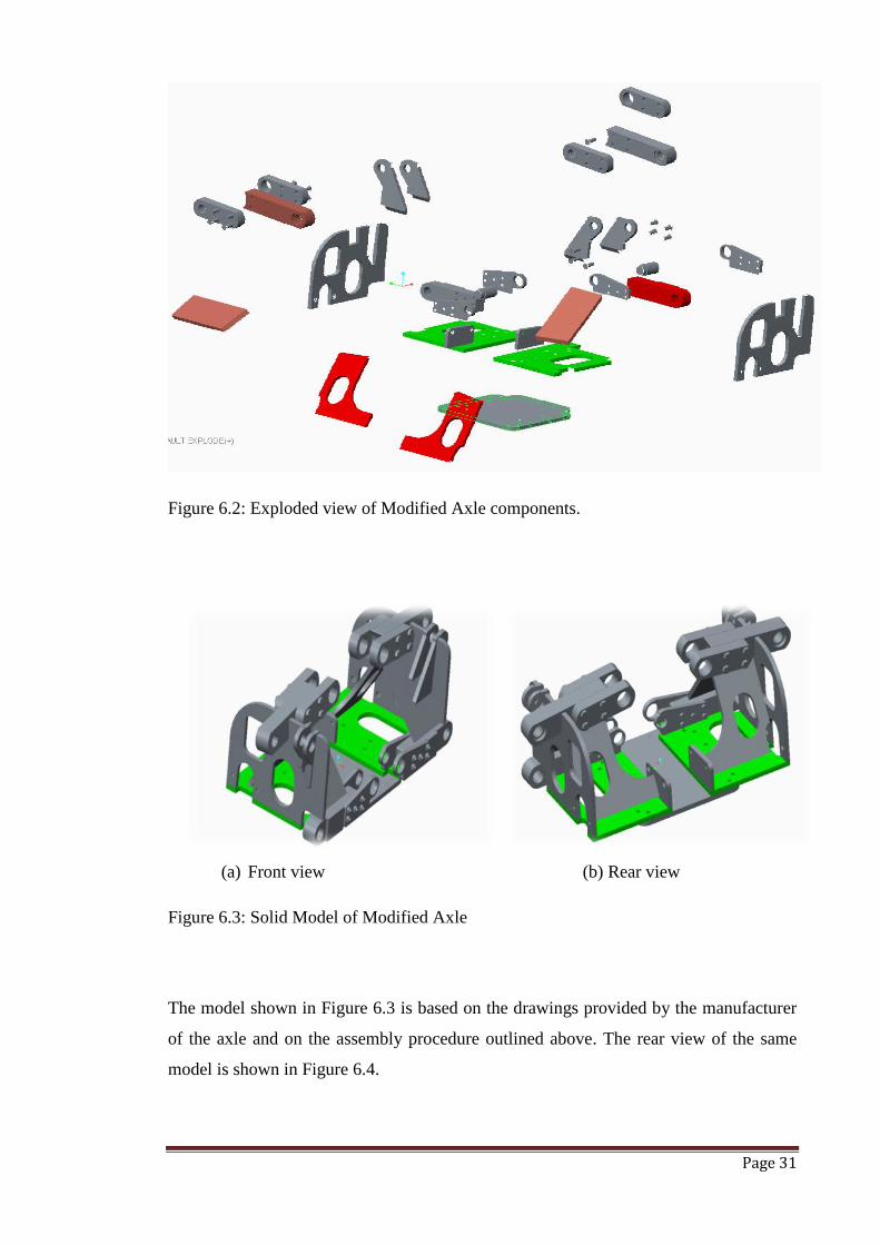
Figure 6.2: Exploded view of Modified Axle components.
(a) Front view (b) Rear view
Figure 6.3: Solid Model of Modified Axle
The model shown in Figure 6.3 is based on the drawings provided by the manufacturer
of the axle and on the assembly procedure outlined above. The rear view of the same
model is shown in Figure 6.4.
Page 32
7.0 FE Analysis- Static Structural Analysis
As previously stated, the major assumption made for this analysis was that the effect of
tyres and hydraulic suspension ram were not considered in the analysis. There are three
stages or processes involved in the static and structural analysis of the component.
These are namely pre-processing, processing and post processing. In pre-processing the
axle model is set up for analysis by converting it into a finite element model by adding
and defining some or all of the following finite element model characteristics. The
characteristics defined for the model include the geometry of the model, material used
in the model and its properties, type of elements, meshing, boundary conditions or
constraints and the loads applied. Once the setting up or pre-processing was completed
the model was then subjected to a static and structural analysis and this stage of analysis
is known as processing. In processing, convergence and outputs are set and these are
discussed in more detail in subsection 7.2.--. Post processing was the final stage of
analysis where the results of the analysis were analysed, factor of safety calculated and
plots of different loading cases and deformed axle model were created.
7.1 Pre-processing
In pre-processing the axle model is set up for analysis by converting it into a finite
element model by adding and defining some or all of the following finite element model
characteristics. The characteristics which defined the model including the geometry of
the model, material used in the model and its properties, type of elements, meshing,
boundary conditions or constraints and the loads applied bare discussed in more detail
in the subsections below.
7.1.1 Geometry
The 3D solid geometry of the modified axle was created in Creo 2.0 Parametric as
shown in the previous chapter. Once imported into Creo Simulate the geometry had to
be checked and confirmed.
7.1.2 Element/Model type
In Creo 2.0 Simulate under the home page, model setup icon was chosen and Advanced
tab was selected for the model setup window. Confirmed that 3D option was checked
and the bonded default interface is also selected.
Page 33
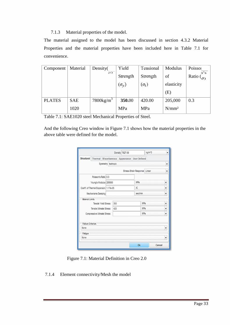
7.1.3 Material properties of the model.
The material assigned to the model has been discussed in section 4.3.2 Material
Properties and the material properties have been included here in Table 7.1 for
convenience.
Component Material Density( ) Yield
Strength
( )Tensional
Strength
( )
Modulus
of
elasticity
(E)
Poisson’s
Ratio ( )
PLATES SAE
1020
7800kg/m3 350.00
MPa
420.00
MPa
205,000
N/mm²
0.3
Table 7.1: SAE1020 steel Mechanical Properties of Steel.
And the following Creo window in Figure 7.1 shows how the material properties in theabove table were defined for the model.
Figure 7.1: Material Definition in Creo 2.0
7.1.4 Element connectivity/Mesh the model

Page 34
The model’s elements were connected or meshed using meshing for solids known as
tetrahedral elements. The mesh was also automatically generated in the running mode.
The difference between a fine meshed and a coarse meshed component is shown in the
Figure 7.2 below. Toogood, R (2012) noted that the density of the mesh in Creo does
not have a large effect on the final solution of an analysis. The running time of the
analysis though can be hugely affected.
(a) Auto meshed (b) Fine meshed
Figure 7.2: Finite Element Model of modified Axle
7.1.5 Boundary conditions
The details of the loads applied on the model were calculated and given in the next
section and in Appendix-A. A typical model showing loads and boundary conditions is
given in Figure 7.3 below. The fixed constraint was applied to the inner mounting
points of the model which are used to mount the modified axle to the tractor block or
chassis. There should be no movement between these two parts and all movement
especially of the wishbones and the hydraulic ram should be restricted to the outer
mounting ends of the axle. That is the reason bearing loadings were applied on these
outer mounting points to cater for such movement.

Page 35
Figure 7.3: FE Model of Modified tractor Axle showing constraints and loadings
7.1.6 Overview of Tests and Loading conditions.
Distribution of weight distribution between the front and rear wheels of the tractor had
to be considered in evaluation of the actual loadings on the modified front axle. A
Canadian government department of Agriculture and development developed a guide on
how to evaluate the weight distribution between the front and the rear wheel. The
weight distribution depends on type of the tractor especially the type of drive. The table
below shows the weight distribution as a percentage for the different types of tractors.
These were considered using total ballasted weight or the working weight of the
tractors.
Tractor drive type Front Axle Rear Axle
2WD 30% 70%
4WD 55% 45%
FWA 40% 60%
Table 7.2: Tractor axle weight distribution
LOADS APPLIED
AT THESE POINTS
CONSTRAINTS
APPLIED AT THESE
POINTS
Page 36
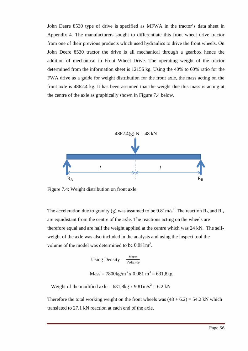
John Deere 8530 type of drive is specified as MFWA in the tractor’s data sheet in
Appendix 4. The manufacturers sought to differentiate this front wheel drive tractor
from one of their previous products which used hydraulics to drive the front wheels. On
John Deere 8530 tractor the drive is all mechanical through a gearbox hence the
addition of mechanical in Front Wheel Drive. The operating weight of the tractor
determined from the information sheet is 12156 kg. Using the 40% to 60% ratio for the
FWA drive as a guide for weight distribution for the front axle, the mass acting on the
front axle is 4862.4 kg. It has been assumed that the weight due this mass is acting at
the centre of the axle as graphically shown in Figure 7.4 below.
4862.4(g) N = 48 kN
l l
RA RB
Figure 7.4: Weight distribution on front axle.
The acceleration due to gravity (g) was assumed to be 9.81m/s2. The reaction RA and RB
are equidistant from the centre of the axle. The reactions acting on the wheels are
therefore equal and are half the weight applied at the centre which was 24 kN. The self-
weight of the axle was also included in the analysis and using the inspect tool the
volume of the model was determined to be 0.081m3.
Using Density =
Mass = 7800kg/m3 x 0.081 m3 = 631,8kg.
Weight of the modified axle = 631,8kg x 9.81m/s2 = 6.2 kN
Therefore the total working weight on the front wheels was (48 + 6.2) = 54.2 kN which
translated to 27.1 kN reaction at each end of the axle.
Page 37
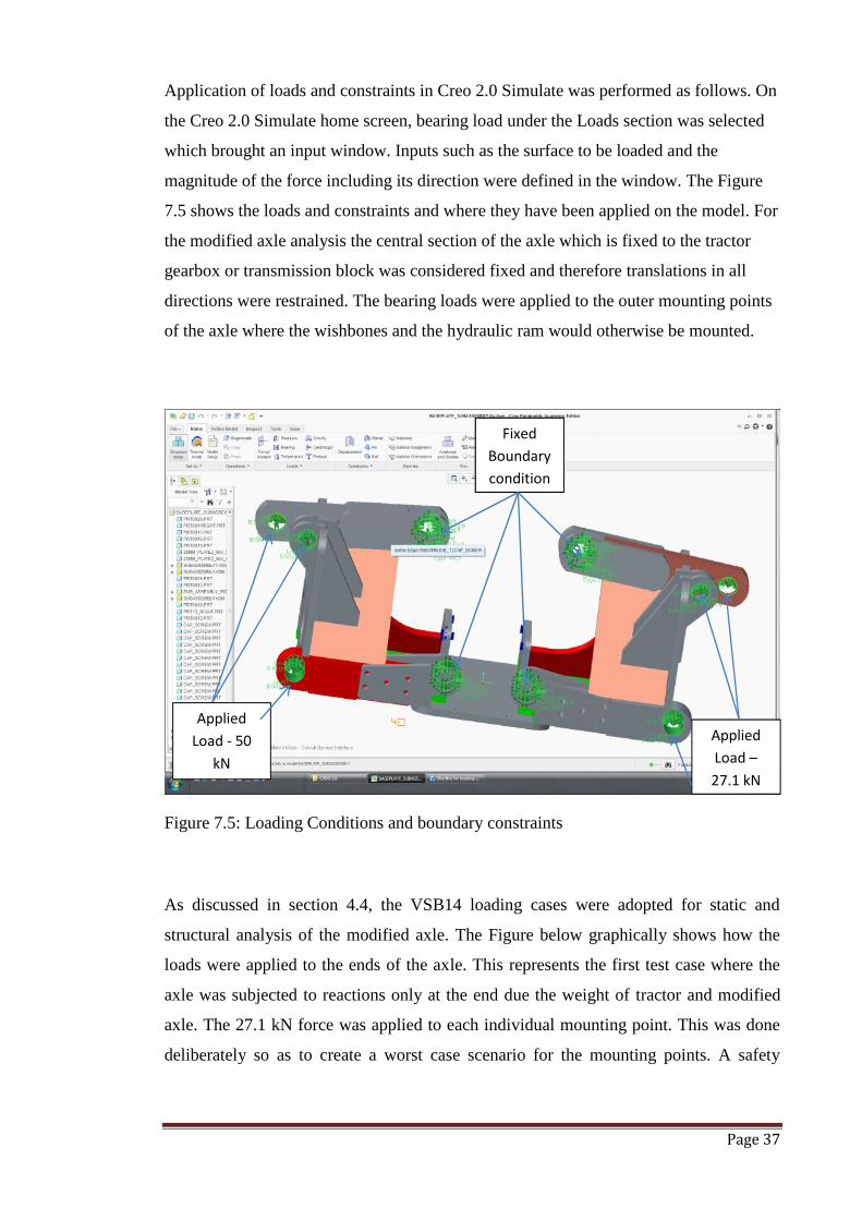
Application of loads and constraints in Creo 2.0 Simulate was performed as follows. On
the Creo 2.0 Simulate home screen, bearing load under the Loads section was selected
which brought an input window. Inputs such as the surface to be loaded and the
magnitude of the force including its direction were defined in the window. The Figure
7.5 shows the loads and constraints and where they have been applied on the model. For
the modified axle analysis the central section of the axle which is fixed to the tractor
gearbox or transmission block was considered fixed and therefore translations in all
directions were restrained. The bearing loads were applied to the outer mounting points
of the axle where the wishbones and the hydraulic ram would otherwise be mounted.
Figure 7.5: Loading Conditions and boundary constraints
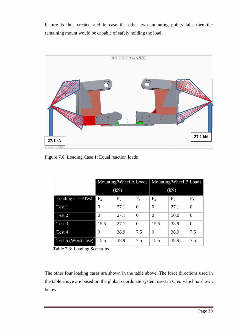
As discussed in section 4.4, the VSB14 loading cases were adopted for static and
structural analysis of the modified axle. The Figure below graphically shows how the
loads were applied to the ends of the axle. This represents the first test case where the
axle was subjected to reactions only at the end due the weight of tractor and modified
axle. The 27.1 kN force was applied to each individual mounting point. This was done
deliberately so as to create a worst case scenario for the mounting points. A safety
FixedBoundarycondition
AppliedLoad - 50
kN
AppliedLoad –27.1 kN
Page 38
feature is thus created and in case the other two mounting points fails then the
remaining mount would be capable of safely holding the load.
Figure 7.6: Loading Case 1: Equal reaction loads
Mounting/Wheel A Loads
(kN)
Mounting/Wheel B Loads
(kN)
Loading Case/Test Fx Fy Fz Fx Fy Fz
Test 1 0 27.1 0 0 27.1 0
Test 2 0 27.1 0 0 50.0 0
Test 3 15.5 27.1 0 15.5 38.9 0
Test 4 0 38.9 7.5 0 38.9 7.5
Test 5 (Worst case) 15.5 38.9 7.5 15.5 38.9 7.5
Table 7.3: Loading Scenarios.
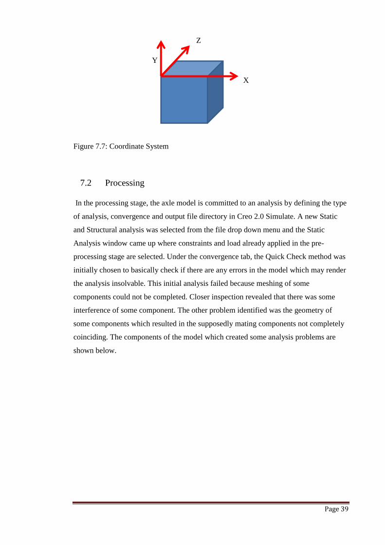
The other four loading cases are shown in the table above. The force directions used in
the table above are based on the global coordinate system used in Creo which is shown
below.
27.1 kN27.1 kN
Page 39
Z
Y
X
Figure 7.7: Coordinate System
7.2 Processing
In the processing stage, the axle model is committed to an analysis by defining the type
of analysis, convergence and output file directory in Creo 2.0 Simulate. A new Static
and Structural analysis was selected from the file drop down menu and the Static
Analysis window came up where constraints and load already applied in the pre-
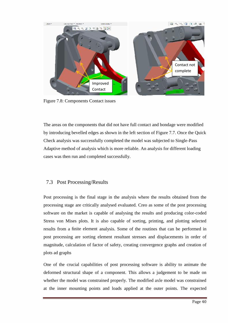
processing stage are selected. Under the convergence tab, the Quick Check method was
initially chosen to basically check if there are any errors in the model which may render
the analysis insolvable. This initial analysis failed because meshing of some
components could not be completed. Closer inspection revealed that there was some
interference of some component. The other problem identified was the geometry of
some components which resulted in the supposedly mating components not completely
coinciding. The components of the model which created some analysis problems are
shown below.
Page 40
Figure 7.8: Components Contact issues
The areas on the components that did not have full contact and bondage were modified
by introducing bevelled edges as shown in the left section of Figure 7.7. Once the Quick
Check analysis was successfully completed the model was subjected to Single-Pass
Adaptive method of analysis which is more reliable. An analysis for different loading
cases was then run and completed successfully.
7.3 Post Processing/Results
Post processing is the final stage in the analysis where the results obtained from the
processing stage are critically analysed evaluated. Creo as some of the post processing
software on the market is capable of analysing the results and producing color-coded
Stress von Mises plots. It is also capable of sorting, printing, and plotting selected
results from a finite element analysis. Some of the routines that can be performed in
post processing are sorting element resultant stresses and displacements in order of
magnitude, calculation of factor of safety, creating convergence graphs and creation of
plots ad graphs
One of the crucial capabilities of post processing software is ability to animate the
deformed structural shape of a component. This allows a judgement to be made on
whether the model was constrained properly. The modified axle model was constrained
at the inner mounting points and loads applied at the outer points. The expected
Contact notcomplete
ImprovedContact
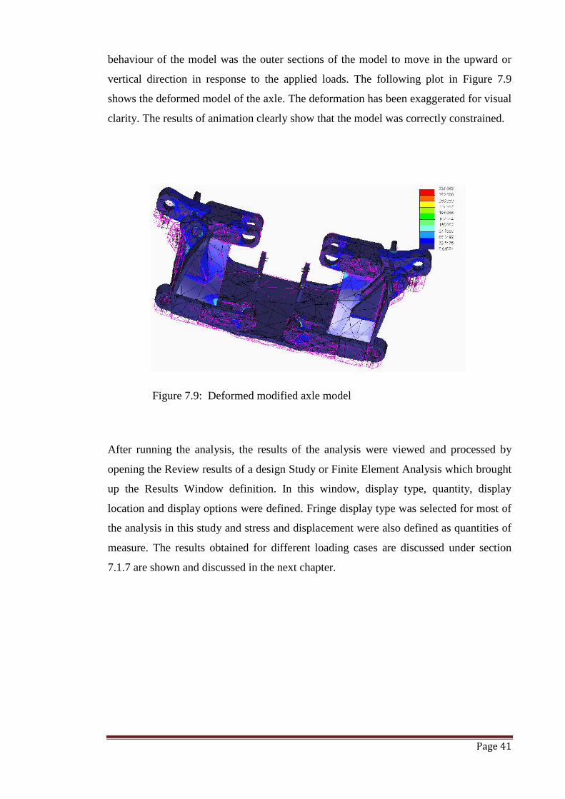
Page 41
behaviour of the model was the outer sections of the model to move in the upward or
vertical direction in response to the applied loads. The following plot in Figure 7.9
shows the deformed model of the axle. The deformation has been exaggerated for visual
clarity. The results of animation clearly show that the model was correctly constrained.
Figure 7.9: Deformed modified axle model
After running the analysis, the results of the analysis were viewed and processed by
opening the Review results of a design Study or Finite Element Analysis which brought
up the Results Window definition. In this window, display type, quantity, display
location and display options were defined. Fringe display type was selected for most of
the analysis in this study and stress and displacement were also defined as quantities of
measure. The results obtained for different loading cases are discussed under section
7.1.7 are shown and discussed in the next chapter.
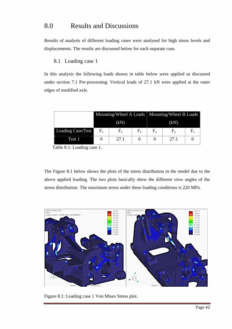
Page 42
8.0 Results and Discussions
Results of analysis of different loading cases were analysed for high stress levels and
displacements. The results are discussed below for each separate case.
8.1 Loading case 1
In this analysis the following loads shown in table below were applied as discussed
under section 7.1 Pre-processing. Vertical loads of 27.1 kN were applied at the outer
edges of modified axle.
Mounting/Wheel A Loads
(kN)
Mounting/Wheel B Loads
(kN)
Loading Case/Test Fx Fy Fz Fx Fy Fz
Test 1 0 27.1 0 0 27.1 0
Table 8.1: Loading case 1.
The Figure 8.1 below shows the plots of the stress distribution in the model due to the
above applied loading. The two plots basically show the different view angles of the
stress distribution. The maximum stress under these loading conditions is 220 MPa.
Figure 8.1: Loading case 1 Von Mises Stress plot.
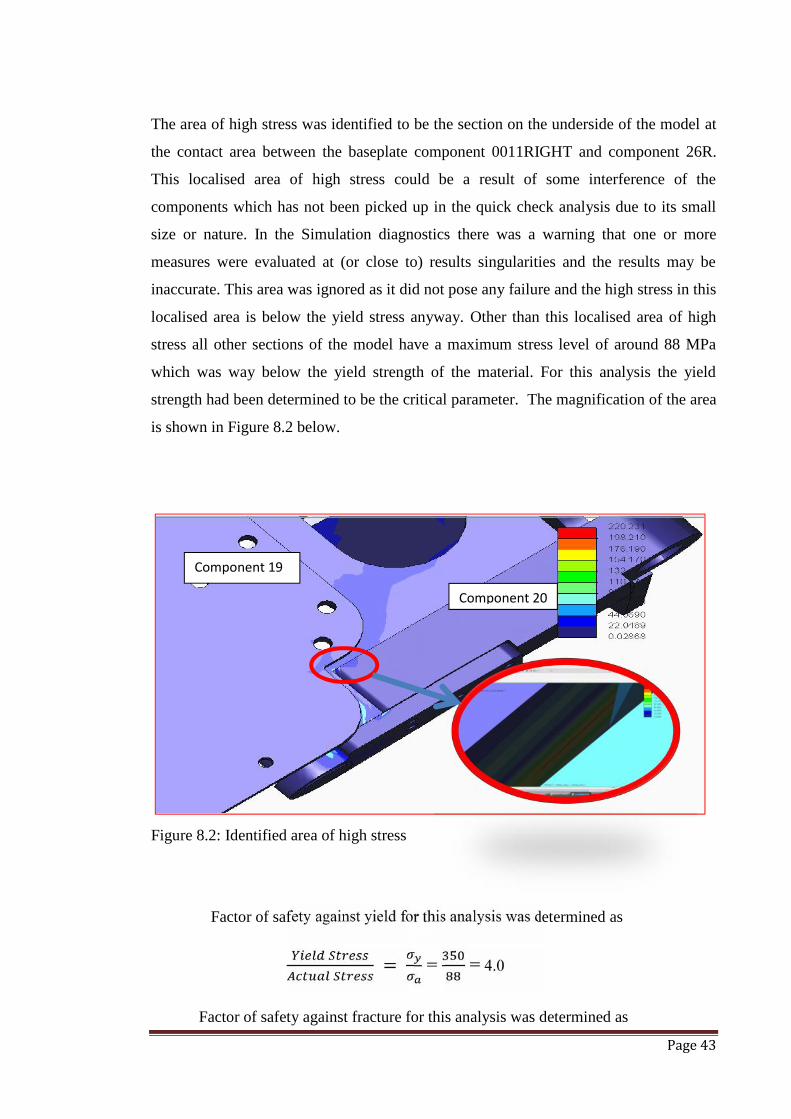
Page 43
The area of high stress was identified to be the section on the underside of the model at
the contact area between the baseplate component 0011RIGHT and component 26R.
This localised area of high stress could be a result of some interference of the
components which has not been picked up in the quick check analysis due to its small
size or nature. In the Simulation diagnostics there was a warning that one or more
measures were evaluated at (or close to) results singularities and the results may be
inaccurate. This area was ignored as it did not pose any failure and the high stress in this
localised area is below the yield stress anyway. Other than this localised area of high
stress all other sections of the model have a maximum stress level of around 88 MPa
which was way below the yield strength of the material. For this analysis the yield
strength had been determined to be the critical parameter. The magnification of the area
is shown in Figure 8.2 below.
Figure 8.2: Identified area of high stress
Factor of safety against yield for this analysis was determined as= = = 4.0
Factor of safety against fracture for this analysis was determined as
Component 19
Component 20
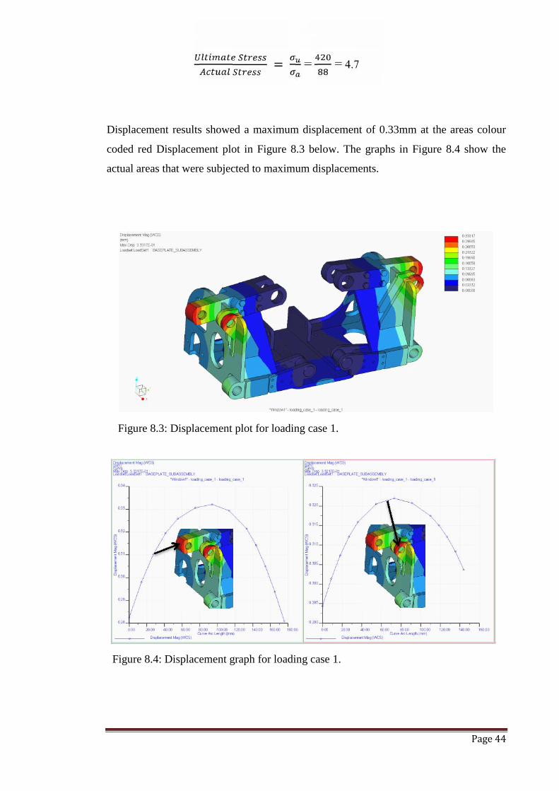
Page 44
= = = 4.7
Displacement results showed a maximum displacement of 0.33mm at the areas colour
coded red Displacement plot in Figure 8.3 below. The graphs in Figure 8.4 show the
actual areas that were subjected to maximum displacements.
Figure 8.3: Displacement plot for loading case 1.
Figure 8.4: Displacement graph for loading case 1.
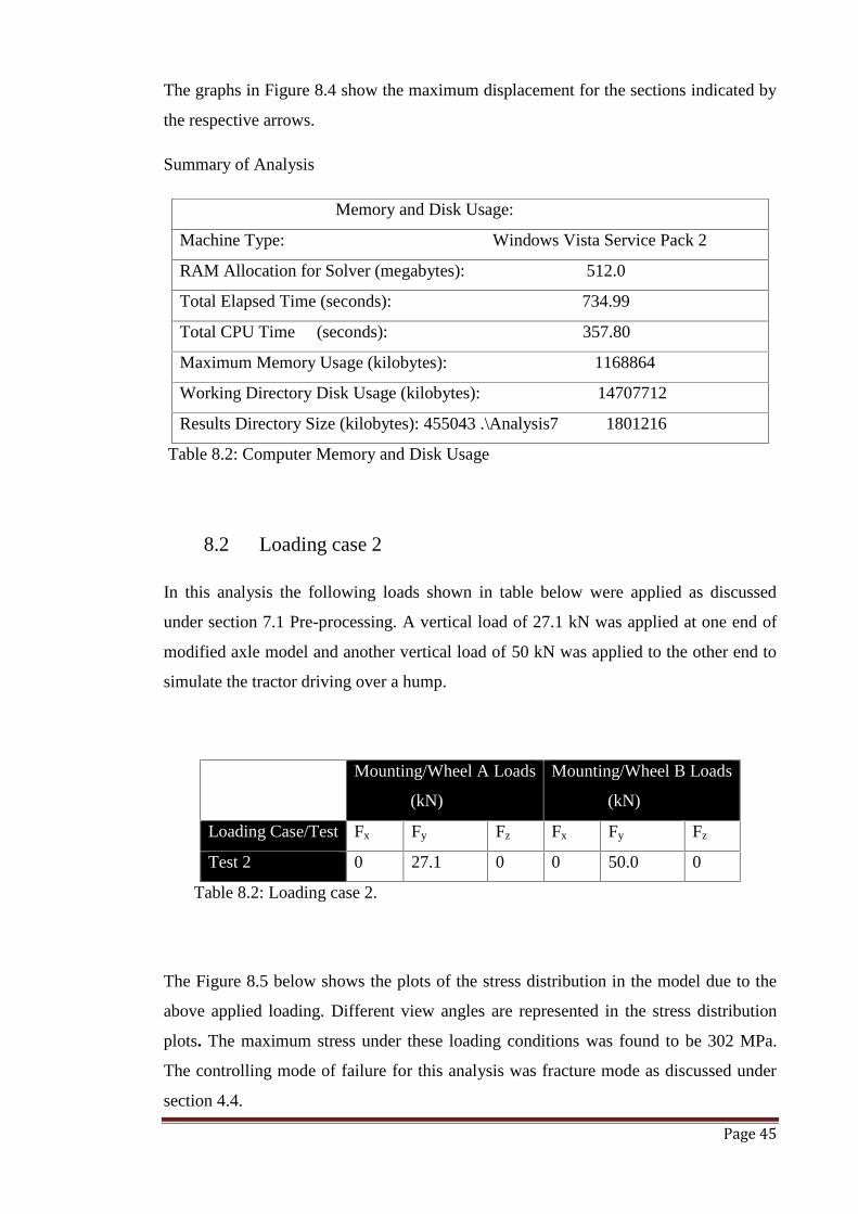
Page 45
The graphs in Figure 8.4 show the maximum displacement for the sections indicated by
the respective arrows.
Summary of Analysis
Table 8.2: Computer Memory and Disk Usage
8.2 Loading case 2
In this analysis the following loads shown in table below were applied as discussed
under section 7.1 Pre-processing. A vertical load of 27.1 kN was applied at one end of
modified axle model and another vertical load of 50 kN was applied to the other end to
simulate the tractor driving over a hump.
Mounting/Wheel A Loads
(kN)
Mounting/Wheel B Loads
(kN)
Loading Case/Test Fx Fy Fz Fx Fy Fz
Test 2 0 27.1 0 0 50.0 0
Table 8.2: Loading case 2.
The Figure 8.5 below shows the plots of the stress distribution in the model due to the
above applied loading. Different view angles are represented in the stress distribution
plots. The maximum stress under these loading conditions was found to be 302 MPa.
The controlling mode of failure for this analysis was fracture mode as discussed under
section 4.4.
Memory and Disk Usage:
Machine Type: Windows Vista Service Pack 2
RAM Allocation for Solver (megabytes): 512.0
Total Elapsed Time (seconds): 734.99
Total CPU Time (seconds): 357.80
Maximum Memory Usage (kilobytes): 1168864
Working Directory Disk Usage (kilobytes): 14707712
Results Directory Size (kilobytes): 455043 .\Analysis7 1801216
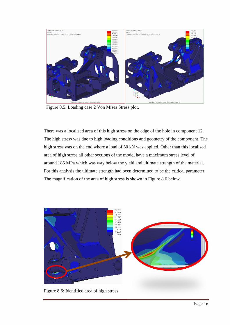
Page 46
Figure 8.5: Loading case 2 Von Mises Stress plot.
There was a localised area of this high stress on the edge of the hole in component 12.
The high stress was due to high loading conditions and geometry of the component. The
high stress was on the end where a load of 50 kN was applied. Other than this localised
area of high stress all other sections of the model have a maximum stress level of
around 185 MPa which was way below the yield and ultimate strength of the material.
For this analysis the ultimate strength had been determined to be the critical parameter.
The magnification of the area of high stress is shown in Figure 8.6 below.
Figure 8.6: Identified area of high stress
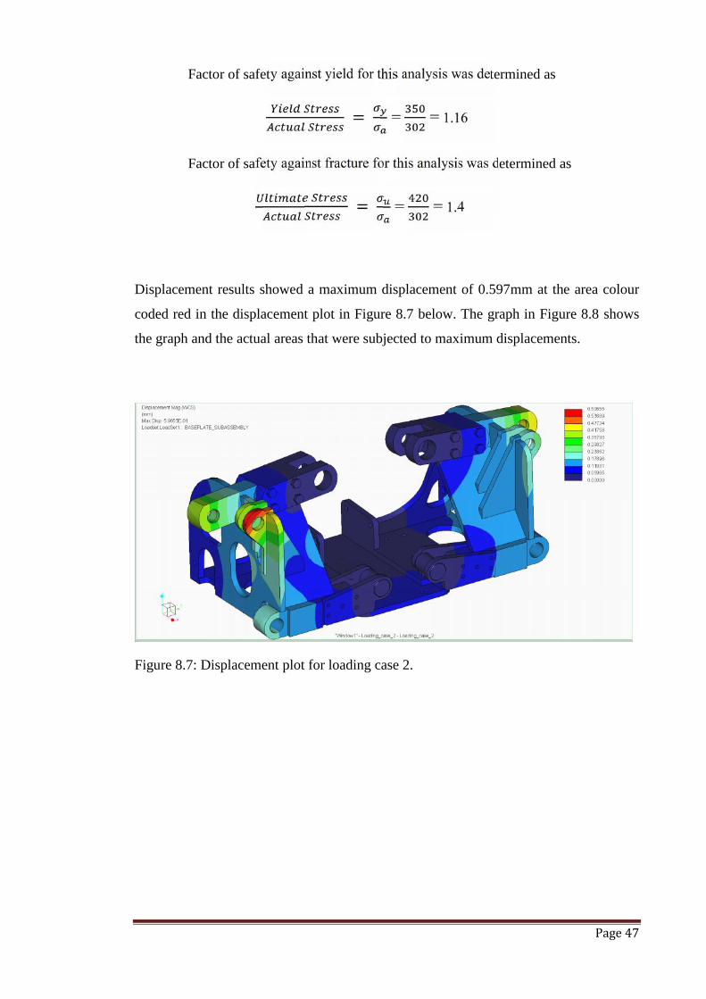
Page 47
Factor of safety against yield for this analysis was determined as= = = 1.16
Factor of safety against fracture for this analysis was determined as= = = 1.4
Displacement results showed a maximum displacement of 0.597mm at the area colour
coded red in the displacement plot in Figure 8.7 below. The graph in Figure 8.8 shows
the graph and the actual areas that were subjected to maximum displacements.
Figure 8.7: Displacement plot for loading case 2.
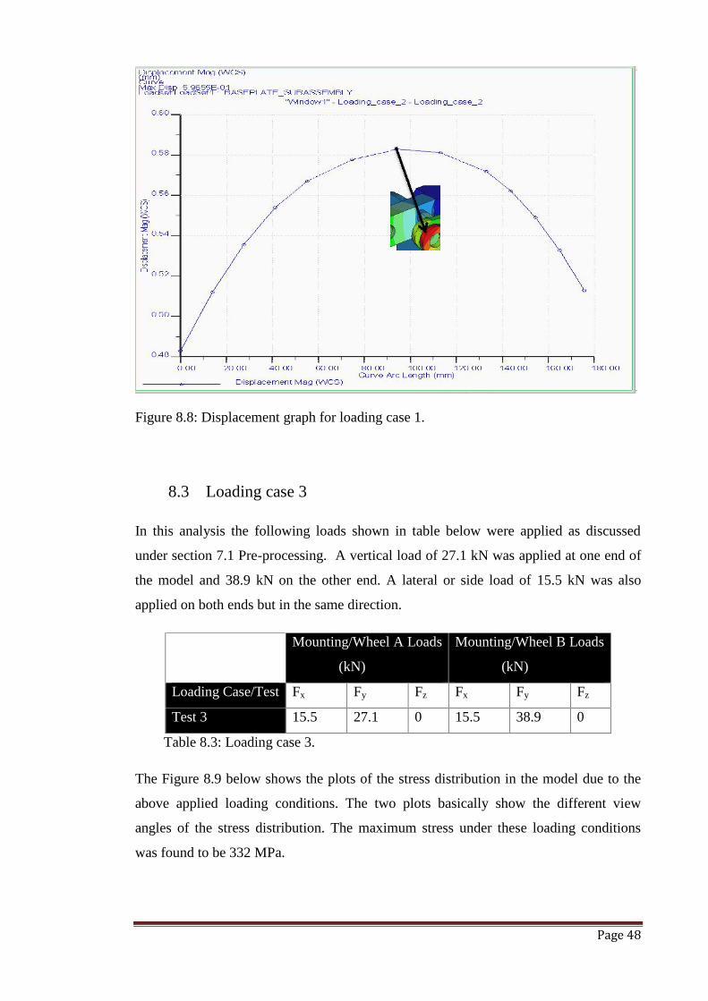
Page 48
Figure 8.8: Displacement graph for loading case 1.
8.3 Loading case 3
In this analysis the following loads shown in table below were applied as discussed
under section 7.1 Pre-processing. A vertical load of 27.1 kN was applied at one end of
the model and 38.9 kN on the other end. A lateral or side load of 15.5 kN was also
applied on both ends but in the same direction.
Mounting/Wheel A Loads
(kN)
Mounting/Wheel B Loads
(kN)
Loading Case/Test Fx Fy Fz Fx Fy Fz
Test 3 15.5 27.1 0 15.5 38.9 0
Table 8.3: Loading case 3.
The Figure 8.9 below shows the plots of the stress distribution in the model due to the
above applied loading conditions. The two plots basically show the different view
angles of the stress distribution. The maximum stress under these loading conditions
was found to be 332 MPa.
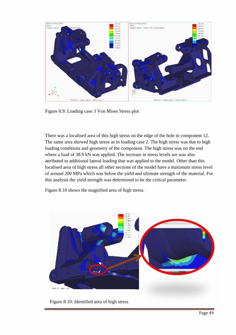
Page 49
Figure 8.9: Loading case 3 Von Mises Stress plot
There was a localised area of this high stress on the edge of the hole in component 12.The same area showed high stress as in loading case 2. The high stress was due to highloading conditions and geometry of the component. The high stress was on the endwhere a load of 38.9 kN was applied. The increase in stress levels are was alsoattributed to additional lateral loading that was applied to the model. Other than thislocalised area of high stress all other sections of the model have a maximum stress levelof around 200 MPa which was below the yield and ultimate strength of the material. Forthis analysis the yield strength was determined to be the critical parameter.
Figure 8.10 shows the magnified area of high stress.
Figure 8.10: Identified area of high stress
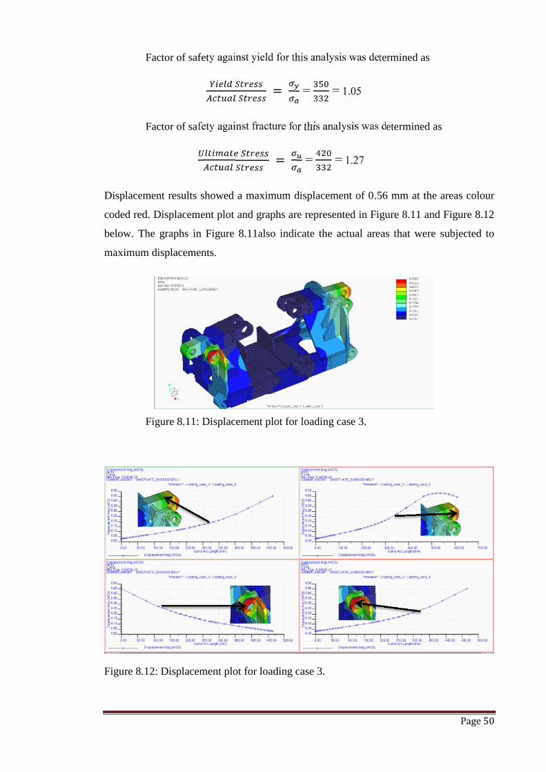
Page 50
Factor of safety against yield for this analysis was determined as= = = 1.05
Factor of safety against fracture for this analysis was determined as= = = 1.27
Displacement results showed a maximum displacement of 0.56 mm at the areas colour
coded red. Displacement plot and graphs are represented in Figure 8.11 and Figure 8.12
below. The graphs in Figure 8.11also indicate the actual areas that were subjected to
maximum displacements.
Figure 8.11: Displacement plot for loading case 3.
Figure 8.12: Displacement plot for loading case 3.
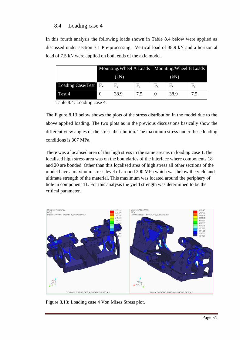
Page 51
8.4 Loading case 4
In this fourth analysis the following loads shown in Table 8.4 below were applied as
discussed under section 7.1 Pre-processing. Vertical load of 38.9 kN and a horizontal
load of 7.5 kN were applied on both ends of the axle model.
Mounting/Wheel A Loads
(kN)
Mounting/Wheel B Loads
(kN)
Loading Case/Test Fx Fy Fz Fx Fy Fz
Test 4 0 38.9 7.5 0 38.9 7.5
Table 8.4: Loading case 4.
The Figure 8.13 below shows the plots of the stress distribution in the model due to the
above applied loading. The two plots as in the previous discussions basically show the
different view angles of the stress distribution. The maximum stress under these loading
conditions is 307 MPa.
There was a localised area of this high stress in the same area as in loading case 1.Thelocalised high stress area was on the boundaries of the interface where components 18and 20 are bonded. Other than this localised area of high stress all other sections of themodel have a maximum stress level of around 200 MPa which was below the yield andultimate strength of the material. This maximum was located around the periphery ofhole in component 11. For this analysis the yield strength was determined to be thecritical parameter.
Figure 8.13: Loading case 4 Von Mises Stress plot.
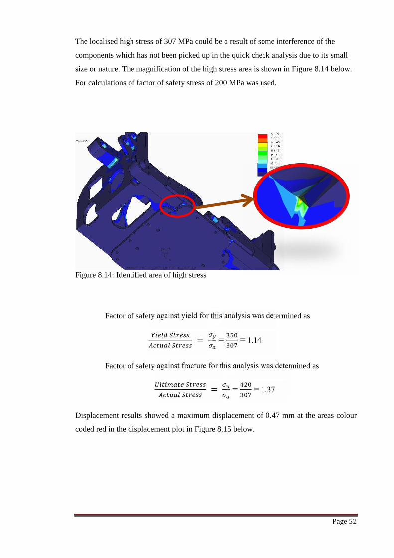
Page 52
The localised high stress of 307 MPa could be a result of some interference of the
components which has not been picked up in the quick check analysis due to its small
size or nature. The magnification of the high stress area is shown in Figure 8.14 below.
For calculations of factor of safety stress of 200 MPa was used.
Figure 8.14: Identified area of high stress
Factor of safety against yield for this analysis was determined as= = = 1.14
Factor of safety against fracture for this analysis was determined as= = = 1.37
Displacement results showed a maximum displacement of 0.47 mm at the areas colour
coded red in the displacement plot in Figure 8.15 below.
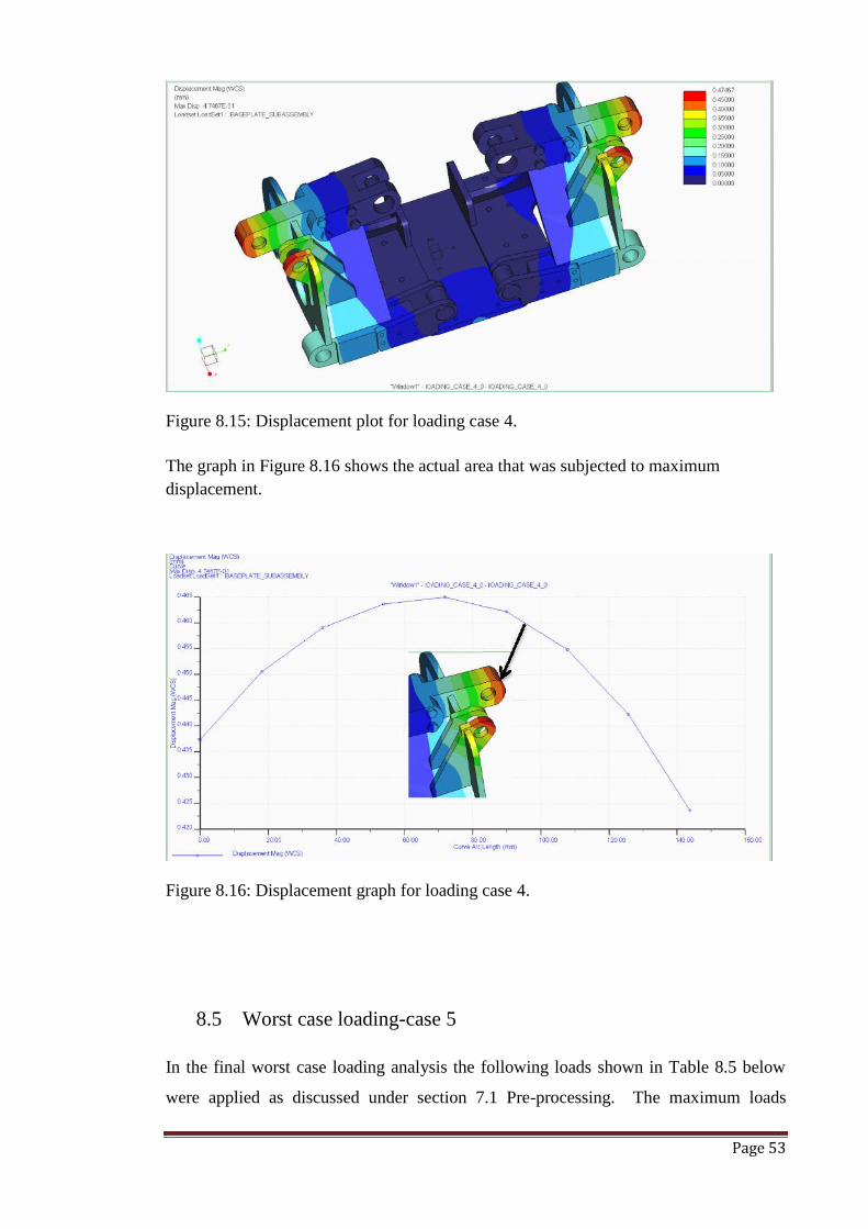
Page 53
Figure 8.15: Displacement plot for loading case 4.
The graph in Figure 8.16 shows the actual area that was subjected to maximumdisplacement.
Figure 8.16: Displacement graph for loading case 4.
8.5 Worst case loading-case 5
In the final worst case loading analysis the following loads shown in Table 8.5 below
were applied as discussed under section 7.1 Pre-processing. The maximum loads
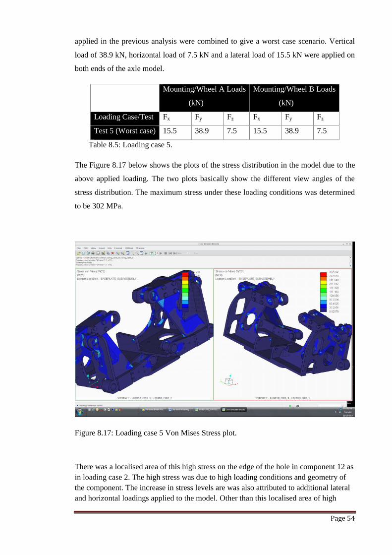
Page 54
applied in the previous analysis were combined to give a worst case scenario. Vertical
load of 38.9 kN, horizontal load of 7.5 kN and a lateral load of 15.5 kN were applied on
both ends of the axle model.
Mounting/Wheel A Loads
(kN)
Mounting/Wheel B Loads
(kN)
Loading Case/Test Fx Fy Fz Fx Fy Fz
Test 5 (Worst case) 15.5 38.9 7.5 15.5 38.9 7.5
Table 8.5: Loading case 5.
The Figure 8.17 below shows the plots of the stress distribution in the model due to the
above applied loading. The two plots basically show the different view angles of the
stress distribution. The maximum stress under these loading conditions was determined
to be 302 MPa.
Figure 8.17: Loading case 5 Von Mises Stress plot.
There was a localised area of this high stress on the edge of the hole in component 12 asin loading case 2. The high stress was due to high loading conditions and geometry ofthe component. The increase in stress levels are was also attributed to additional lateraland horizontal loadings applied to the model. Other than this localised area of high

Page 55
stress all other sections of the model have a maximum stress level of around 168 MPawhich was below the yield and ultimate strength of the material. For this analysis theyield strength was determined to be the critical parameter. This magnification of thearea of high stress is shown in Figure 8.18 below.
Figure 8.18: Identified area of high stress
Factor of safety against yield for this analysis was determined as= = = 1.16
Factor of safety against fracture for this analysis was determined as= = = 1.4
Displacement results showed a maximum displacement of 0.597 mm at the areas colour
coded red Displacement plot in Figure 8.3 below. The graphs in Figure 8.4 show the
actual areas that were subjected to maximum displacements.
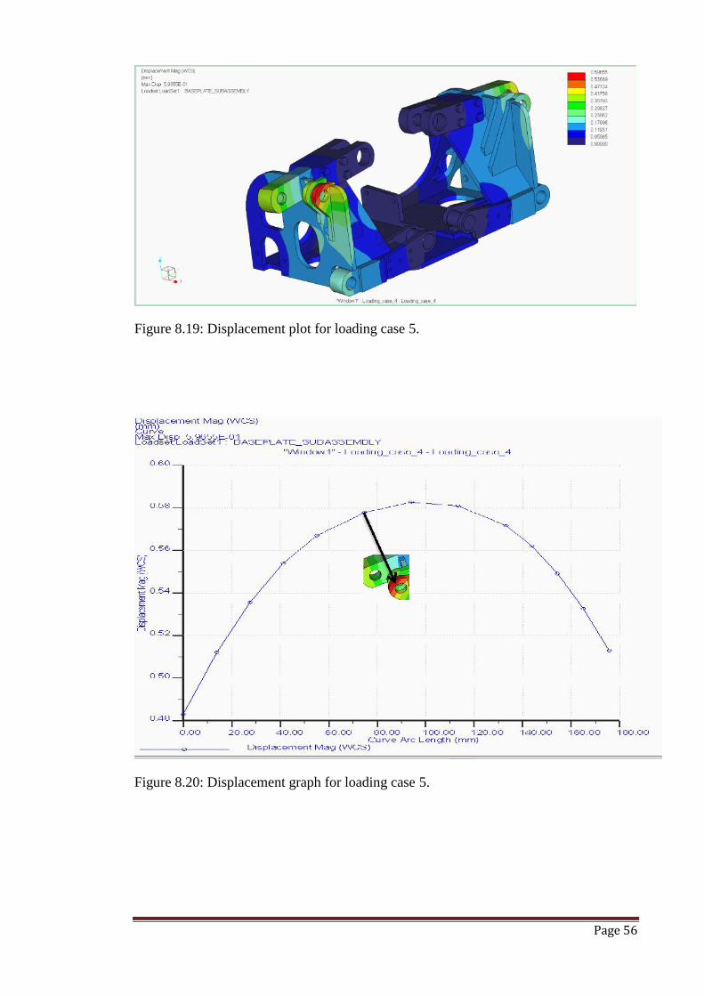
Page 56
Figure 8.19: Displacement plot for loading case 5.
Figure 8.20: Displacement graph for loading case 5.
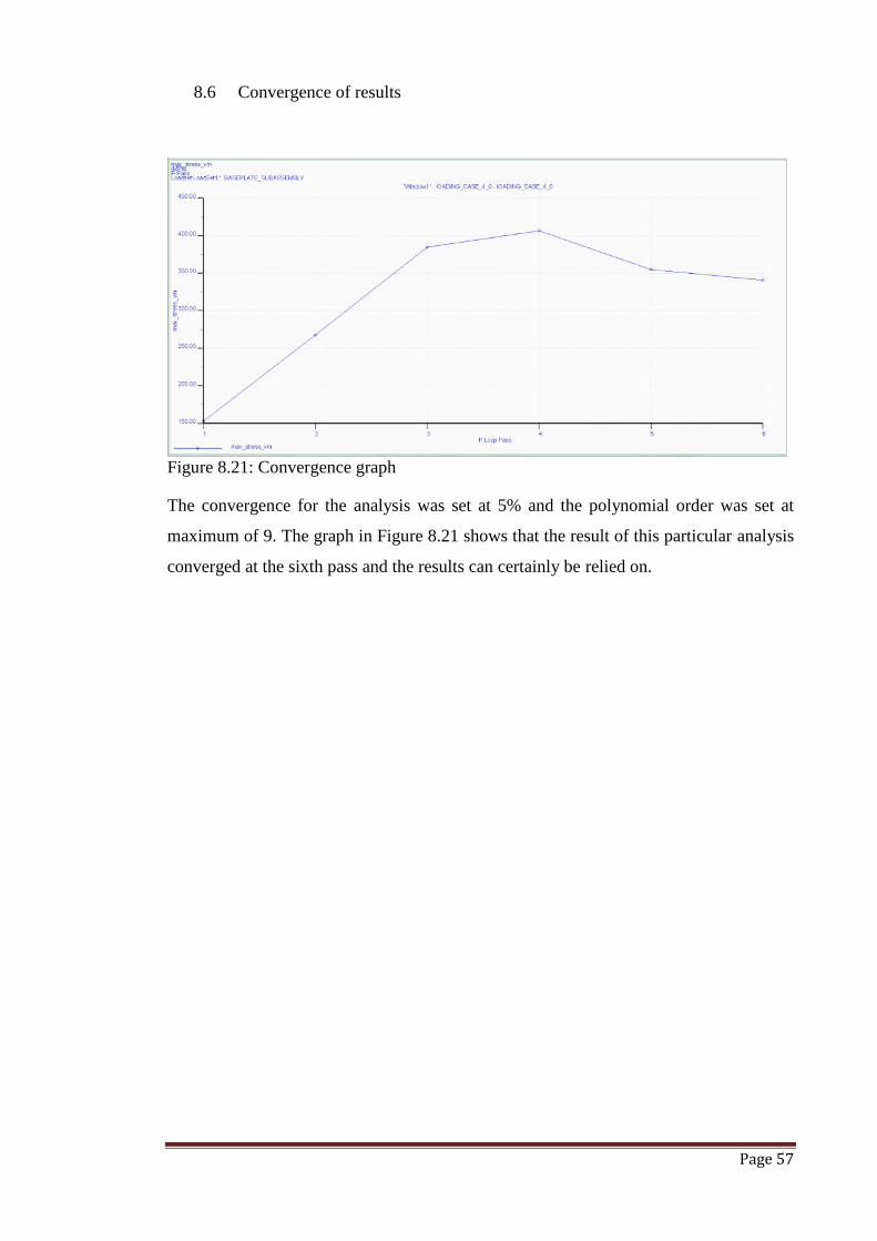
Page 57
8.6 Convergence of results
Figure 8.21: Convergence graph
The convergence for the analysis was set at 5% and the polynomial order was set at
maximum of 9. The graph in Figure 8.21 shows that the result of this particular analysis
converged at the sixth pass and the results can certainly be relied on.

Page 58
9.0 Conclusions and suggestions for future work
Conclusions were drawn based on the results outline in Chapter 8 and a summary of
results and loads applied is shown in the table below.
Mounting/Wheel A Loads
(kN)
Mounting/Wheel B Loads
(kN)
Loading Case/Test Fx Fy Fz Fx Fy Fz
Test 1 0 27.1 0 0 27.1 0
Test 2 0 27.1 0 0 50.0 0
Test 3 15.5 27.1 0 15.5 38.9 0
Test 4 0 38.9 7.5 0 38.9 7.5
Test 5 (Worst case) 15.5 38.9 7.5 15.5 38.9 7.5
Loading
Case/Test
Max Von Mises
Stress (MPa)
Maximum
Displacement
(mm)
FOS(Yield)
FOS(Fracture)
Test 1 220.2 0.33 4 4.7
Test 2 302 0.597 1.16 1.4
Test 3 332 0.56 1.05 1.27
Test 4 307 0.47 1.16 1.37
Test 5 (Worst
case)302 0.597 1.16 1.4
Table 8.1: Summary of Von Mises stress, displacements and factor of safety
Loading case 1 – Loading conditions for this case are safe as the factor of
safety is more than twice the nominal factor of safety calculated for the
model. The factor of safety calculated for the model using the guide in
Appendix G was 1.5.
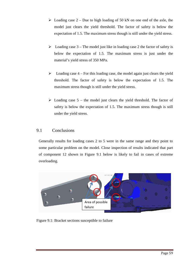
Page 59
Loading case 2 – Due to high loading of 50 kN on one end of the axle, the
model just clears the yield threshold. The factor of safety is below the
expectation of 1.5. The maximum stress though is still under the yield stress.
Loading case 3 – The model just like in loading case 2 the factor of safety is
below the expectation of 1.5. The maximum stress is just under the
material’s yield stress of 350 MPa.
Loading case 4 – For this loading case, the model again just clears the yield
threshold. The factor of safety is below the expectation of 1.5. The
maximum stress though is still under the yield stress.
Loading case 5 – the model just clears the yield threshold. The factor of
safety is below the expectation of 1.5. The maximum stress though is still
under the yield stress.
9.1 Conclusions
Generally results for loading cases 2 to 5 were in the same range and they point to
some particular problem on the model. Close inspection of results indicated that part
of component 12 shown in Figure 9.1 below is likely to fail in cases of extreme
overloading.
Figure 9.1: Bracket sections susceptible to failure
Area of possiblefailure
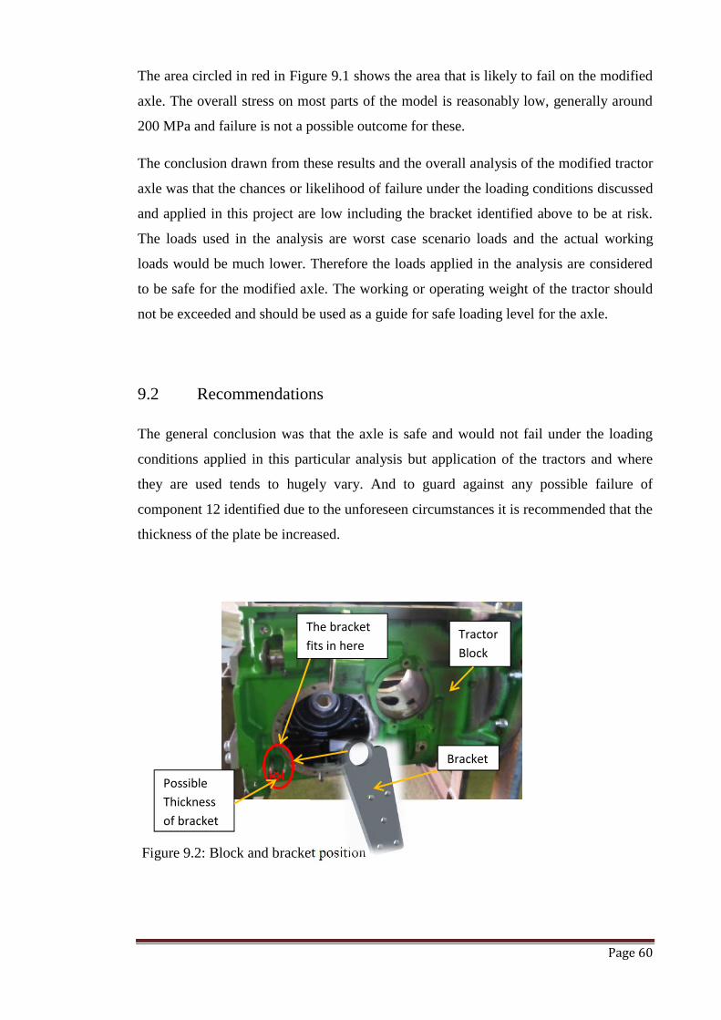
Page 60
The area circled in red in Figure 9.1 shows the area that is likely to fail on the modified
axle. The overall stress on most parts of the model is reasonably low, generally around
200 MPa and failure is not a possible outcome for these.
The conclusion drawn from these results and the overall analysis of the modified tractor
axle was that the chances or likelihood of failure under the loading conditions discussed
and applied in this project are low including the bracket identified above to be at risk.
The loads used in the analysis are worst case scenario loads and the actual working
loads would be much lower. Therefore the loads applied in the analysis are considered
to be safe for the modified axle. The working or operating weight of the tractor should
not be exceeded and should be used as a guide for safe loading level for the axle.
9.2 Recommendations
The general conclusion was that the axle is safe and would not fail under the loading
conditions applied in this particular analysis but application of the tractors and where
they are used tends to hugely vary. And to guard against any possible failure of
component 12 identified due to the unforeseen circumstances it is recommended that the
thickness of the plate be increased.
Figure 9.2: Block and bracket position
The bracketfits in here
PossibleThicknessof bracket
TractorBlock
Bracket
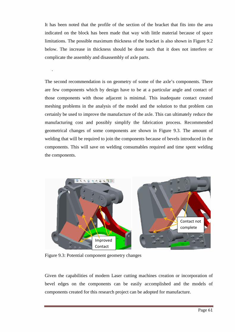
Page 61
It has been noted that the profile of the section of the bracket that fits into the area
indicated on the block has been made that way with little material because of space
limitations. The possible maximum thickness of the bracket is also shown in Figure 9.2
below. The increase in thickness should be done such that it does not interfere or
complicate the assembly and disassembly of axle parts.
.
The second recommendation is on geometry of some of the axle’s components. There
are few components which by design have to be at a particular angle and contact of
those components with those adjacent is minimal. This inadequate contact created
meshing problems in the analysis of the model and the solution to that problem can
certainly be used to improve the manufacture of the axle. This can ultimately reduce the
manufacturing cost and possibly simplify the fabrication process. Recommended
geometrical changes of some components are shown in Figure 9.3. The amount of
welding that will be required to join the components because of bevels introduced in the
components. This will save on welding consumables required and time spent welding
the components.
Figure 9.3: Potential component geometry changes
Given the capabilities of modern Laser cutting machines creation or incorporation of
bevel edges on the components can be easily accomplished and the models of
components created for this research project can be adopted for manufacture.
Contact notcomplete
ImprovedContact
Page 62
9.3 Future Work
Suggestions for future include creation of a parametric model of the modified axle to
suit any similar tractor that might be used for controlled traffic farming. The research
would involve identifying the tractors and verifying the axle’s configuration to
determine if the current model’s parameters could be altered to create a parametric
model.
The effects of the tractor’s independent suspension, linkages such as the wishbones and
the tyres were ignored for the purposes of this research project. Complete analysis of the
axle including these effects of the tyres and independent suspension on the modified
axle is hereby put forward as an area that need further research.
Page 63
10.0 REFERENCES
Adams, V. Do FEA Tools Give The Same Answers? A Comparison of Finite Element
Analysis Software [ONLINE]. Available at:
https://www.clear.rice.edu/mech403/FEA/Compare_FEA_Codes.pdf [Accessed 04
May 2014].
AFGRI Equipment South Africa 2014, AFGRI Equipment, Highveld, Centurion,
viewed 31 July 2014. < http://afgri.johndeeredealer.co.za/John-
Deere/Agriculture2/Tractors/Row-Crop-Tractors/8R-8RT-Series/8285R-Tractor>.
Aloni, S & Khedkar, S 2012, ‘Comparative Evaluation of Tractor Trolley Axle by
Using Finite Element Analysis Approach’, International Journal of Engineering
Science and Technology (IJEST), Vol. 4 No.04, p. 1351.
AZO Materials United Kingdom 2014, AZO Materials, Macclesfield, Cheshire, viewed
30 July 2014. http://www.azom.com/article.aspx?ArticleID=6114
Ballasting Your Tractor for Performance by Alberta Agriculture & Rural Development
2013, A practical guide to proper weighting of your tractor, viewed 04 May 2014,
<http://www1.agric.gov.ab.ca/$Department/deptdocs.nsf/all/eng5240>.
Bowman, K 2008 ‘Economic and Environmental Analysis of Converting to Controlled Traffic
Farming’, Proceedings of the sixth Australian Controlled Traffic Farming Conference, Dubbo,
New South Wales, pp. 61-68.
Buyer’s guide for FEA software Tips to help you select an FEA solution, Siemens
Software, viewed 20 April 2014,
<http://www.mayahtt.com/wpcontent/uploads/2013/04/Buyers-Guide-for-FEA-
Software.pdf>.
EMCH213D Design in Strength of Materials: Tutorial/Instructional Resources 2014,
Pennsylvania State University, Pennsylvania, viewed 17 October 2014,
<http://www.esm.psu.edu>.
Page 64
ENG4111 Project Reference Book 2014, University of Southern Queensland,
Toowoomba.
Implementing a controlled traffic farming system by Grains Research & Development
Corporation 2013, Controlled traffic farming factsheet, viewed 04 May 2014,
<http://www.grdc.com.au/~/media/B1422ABEE81649E2BB3895D2D198099F.pdf>
Jensen, H, G. Jacobsen, L, Pedersen, S, M, Tavella, E 2012, ‘Socioeconomic impact of
widespread adoption of precision farming and controlled traffic systems in Denmark’,
Journal of Precision Agriculture, vol. 13, no. 6, pp. 661-677.
Koyuncu, A, Gökler, M, & Balkan, T, 2012, ‘Development of a design verification
methodology including strength and fatigue life prediction for agricultural tractors’,
International Journal of Advanced Manufacturing Technology, vol. 60, no. 5-8, pp.
777-785.
Larocque, S, 2012 Controlled Traffic Farming. Canada: Office for Official
Publications of the Nuffield Canada.
León, O, N, Martínez, P, Orta C, P. & Adaya 2000, Reducing the weight of a frontal
truck axle beam using experimental test procedures to fine tune FEA. 2nd Worldwide
MSC Automotive Conference. Dearborn, Michigan; October 9-11, 2000 viewed 04 May
2014, <http://web.mscsoftware.com/support/library/conf/auto00/p04300.pdf>.
Logan, D, L 2007, The First Course in the Finite Element Method, Thomson Learning,
United States.
Longhurst, B, 2010 FX-HR Holden Front End Stress Analysis & Geometry Assessment,
Australia: Official Publications of Bremar Automotion Pty Ltd.
Mahanty, D, K Manohar, V, Khomane & B, S, Nayak. S 2002, Analysis and Weight
Reduction of a Tractor’s Front Axle, viewed 04 May 2014,
<http://www.ansys.com/staticassets/ANSYS/staticassets/resourcelibrary/confpaper/200
2-Int-ANSYS-Conf-106.PDF>.
Page 65
Maisuria, M & Patel, D, A 2014 ‘FE Analysis Of Runner Blade For Small Bulb
Turbine’, IOSR Journal of Mechanical and Civil Engineering (IOSR-JMCE) vol. 11, no.
2, version vii, pp. 73-77.
Neale, T, 2010, The Cost of Grain Harvester Compaction, viewed 10 May 2014,
<www.precisionagriculture.com.au/display.php?file=19>.
Tarighi, J, Mohtasebi, S, S & Alimardani, R 2011, ‘Static and dynamic analysis of front axle
housing of tractor using finite element methods’, Australian Journal of Agricultural
Engineering vol. 2, no. 2, pp. 45-49.
Toogood, R 2012, Creo Simulate Tutorial Releases 1.0 & 2.0, Schroff Development
Corporation, Alberta.
Ullman, D, G 2010, The Mechanical Design Process, 4th edn, McGraw-Hill, New
York, viewed 23 August 2014, <http://www.scribd.com/doc/116799665/The-
Mechanical-Design-Process-David-G-Ullman-4-Edition>.
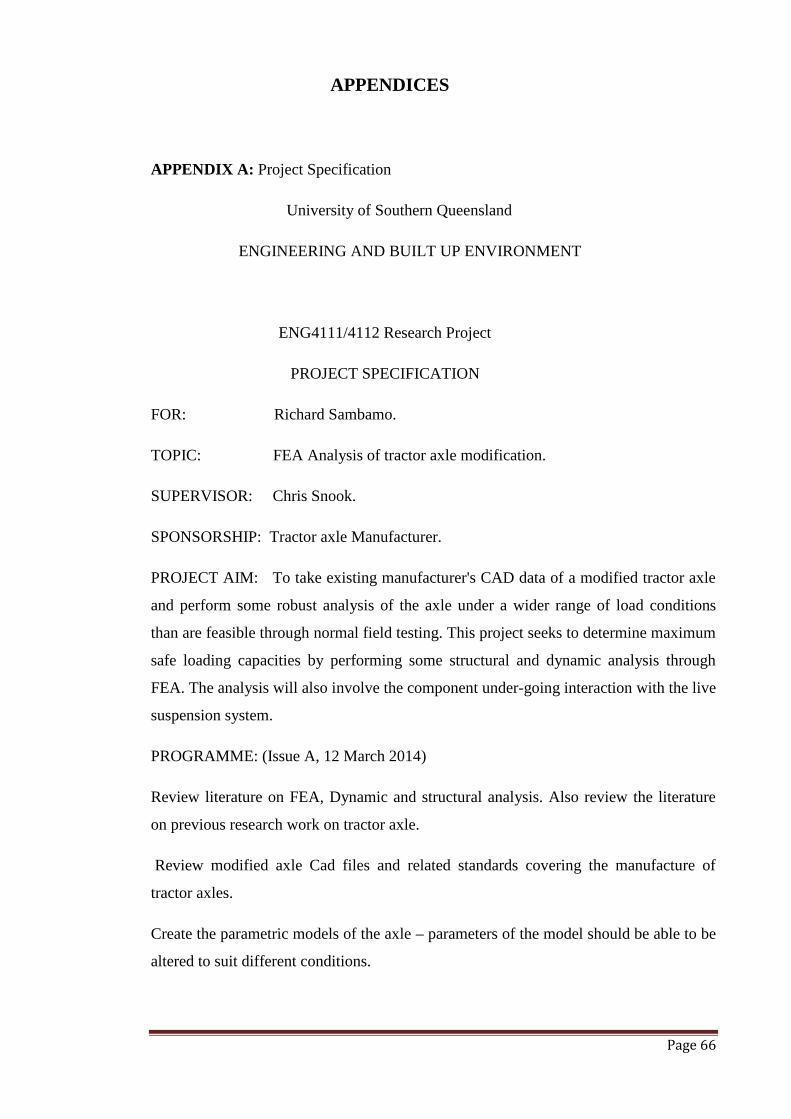
Page 66
APPENDICES
APPENDIX A: Project Specification
University of Southern Queensland
ENGINEERING AND BUILT UP ENVIRONMENT
ENG4111/4112 Research Project
PROJECT SPECIFICATION
FOR: Richard Sambamo.
TOPIC: FEA Analysis of tractor axle modification.
SUPERVISOR: Chris Snook.
SPONSORSHIP: Tractor axle Manufacturer.
PROJECT AIM: To take existing manufacturer's CAD data of a modified tractor axle
and perform some robust analysis of the axle under a wider range of load conditions
than are feasible through normal field testing. This project seeks to determine maximum
safe loading capacities by performing some structural and dynamic analysis through
FEA. The analysis will also involve the component under-going interaction with the live
suspension system.
PROGRAMME: (Issue A, 12 March 2014)
Review literature on FEA, Dynamic and structural analysis. Also review the literature
on previous research work on tractor axle.
Review modified axle Cad files and related standards covering the manufacture of
tractor axles.
Create the parametric models of the axle – parameters of the model should be able to be
altered to suit different conditions.

Page 67
Perform static and modal analysis.
Perform a structural and a dynamic analysis.
Critically review the results of the FEA, structural and dynamic analysis.
Recommendations, conclusions and any further work to be undertaken.
AGREED
(Student Name) (Supervisor Name)
(Signature) (Signature)
/ / (Date) / / (Date)
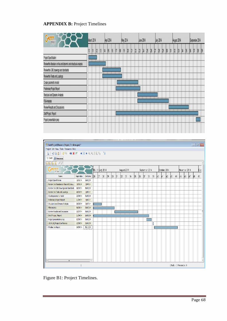
Page 68
APPENDIX B: Project Timelines
Figure B1: Project Timelines.
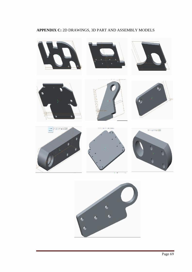
Page 69
APPENDIX C: 2D DRAWINGS, 3D PART AND ASSEMBLY MODELS
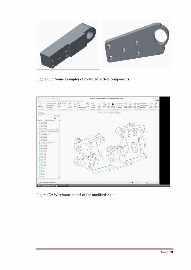
Page 70
Figure C1: Some examples of modified Axle’s components.
Figure C2: Wireframe model of the modified Axle.
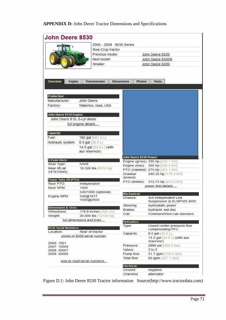
Page 71
APPENDIX D: John Deere Tractor Dimensions and Specifications
Figure D.1: John Deere 8530 Tractor information Source(http://www.tractordata.com)

Page 72
APPENDIX E: Loadings and Constraints
Figure E1: Loadings and constraints on model.
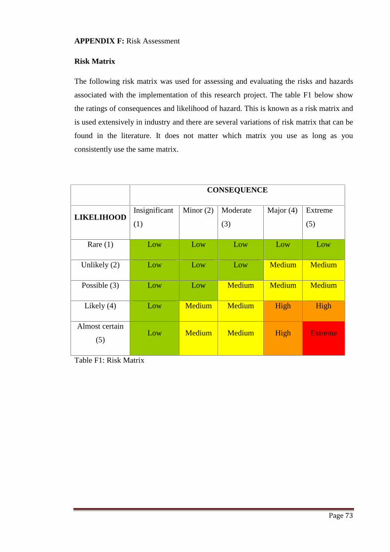
Page 73
APPENDIX F: Risk Assessment
Risk Matrix
The following risk matrix was used for assessing and evaluating the risks and hazards
associated with the implementation of this research project. The table F1 below show
the ratings of consequences and likelihood of hazard. This is known as a risk matrix and
is used extensively in industry and there are several variations of risk matrix that can be
found in the literature. It does not matter which matrix you use as long as you
consistently use the same matrix.
CONSEQUENCE
LIKELIHOODInsignificant
(1)
Minor (2) Moderate
(3)
Major (4) Extreme
(5)
Rare (1) Low Low Low Low Low
Unlikely (2) Low Low Low Medium Medium
Possible (3) Low Low Medium Medium Medium
Likely (4) Low Medium Medium High High
Almost certain
(5)Low Medium Medium High Extreme
Table F1: Risk Matrix
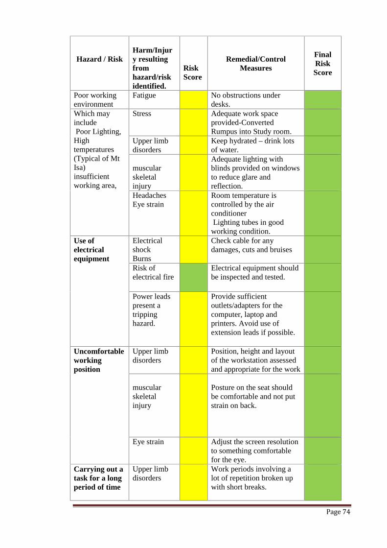
Page 74
Hazard / RiskHarm/Injury resultingfromhazard/riskidentified.
RiskScore
Remedial/ControlMeasures
FinalRiskScore
Poor workingenvironment
Fatigue No obstructions underdesks.
Which mayincludePoor Lighting,Hightemperatures(Typical of MtIsa)insufficientworking area,
Stress Adequate work spaceprovided-ConvertedRumpus into Study room.
Upper limbdisorders
Keep hydrated – drink lotsof water.
muscularskeletalinjury
Adequate lighting withblinds provided on windowsto reduce glare andreflection.
HeadachesEye strain
Room temperature iscontrolled by the airconditionerLighting tubes in good
working condition.Use ofelectricalequipment
ElectricalshockBurns
Check cable for anydamages, cuts and bruises
Risk ofelectrical fire
Electrical equipment shouldbe inspected and tested.
Power leadspresent atrippinghazard.
Provide sufficientoutlets/adapters for thecomputer, laptop andprinters. Avoid use ofextension leads if possible.
Uncomfortableworkingposition
Upper limbdisorders
Position, height and layoutof the workstation assessedand appropriate for the work
muscularskeletalinjury
Posture on the seat shouldbe comfortable and not putstrain on back.
Eye strain Adjust the screen resolutionto something comfortablefor the eye.
Carrying out atask for a longperiod of time
Upper limbdisorders
Work periods involving alot of repetition broken upwith short breaks.
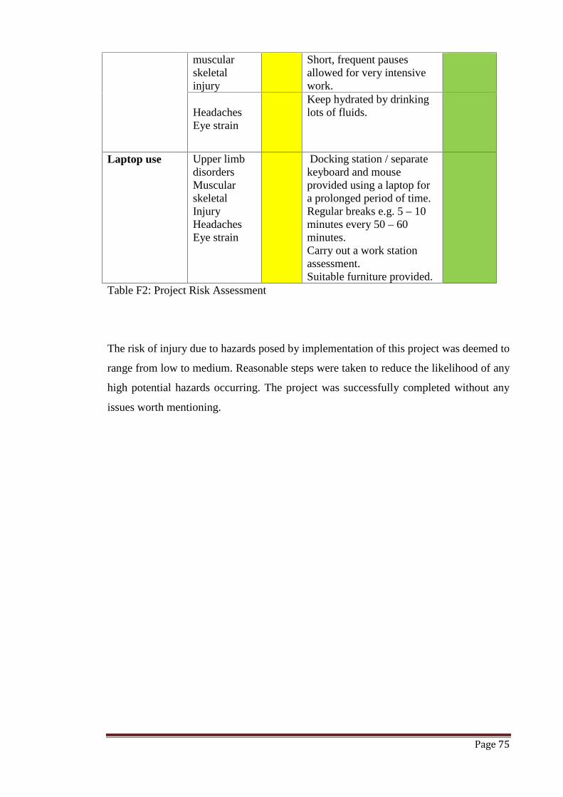
Page 75
muscularskeletalinjury
Short, frequent pausesallowed for very intensivework.
HeadachesEye strain
Keep hydrated by drinkinglots of fluids.
Laptop use Upper limbdisordersMuscularskeletalInjuryHeadachesEye strain
Docking station / separatekeyboard and mouseprovided using a laptop fora prolonged period of time.Regular breaks e.g. 5 – 10minutes every 50 – 60minutes.Carry out a work stationassessment.Suitable furniture provided.
Table F2: Project Risk Assessment
The risk of injury due to hazards posed by implementation of this project was deemed to
range from low to medium. Reasonable steps were taken to reduce the likelihood of any
high potential hazards occurring. The project was successfully completed without any
issues worth mentioning.
Page 76
APPENDIX G: Factor of Safety Calculations
C.2 THE CLASSICAL RULE-OF-THUMBFACTOR OF SAFETY
The factor of safety can be quickly estimated on the basis of estimated variations of the
five measures previously discussed: material properties, stress, geometry, failure
analysis, and desired reliability. The better known the material properties and stress, the
tighter the tolerances, the more accurate and applicable the failure theory, and the lower
the required reliability, the closer the factor of safety should be to 1. The less known
about the material, stress, failure analysis, and geometry and the higher the required
reliability, the larger the factor of safety. The simplest way to present this technique is
to associate a value greater than 1 with each of the measures and define the factor of
safety as the product of these five values:
FS = FSmaterial · FSstress · FSgeometry · FSfailure analysis · FSreliability
Details on how to estimate these five values are given next. These values have been
developed by breaking down the rules given in textbooks and handbooks into the five
measures and cross-checking the values with those from the statistical method described
in Section C.3.
Estimating the Contribution for the Material
FSmaterial =1.0 If the properties for the material are well known, if they have been
experimentally obtained from tests on a specimen known to be identical to the
component being designed and v tests representing the loading to be applied
FSmaterial=1.1 If the material properties are known from a handbook or a
manufacturer’s values FSmaterial=1.2–1.4. If the material properties are not well
known
Estimating the Contribution for the Load Stress
FSstress=1.0–1.1 If the load is well defined as static or fluctuating, if there are no
anticipated overloads or shock loads, and if an accurate method of analysing the stress
has been used
FSstress=1.2–1.3 If the nature of the load is defined in an average manner, with
overloads of 20–50%, and the stress analysis method may result in errors less than 50%
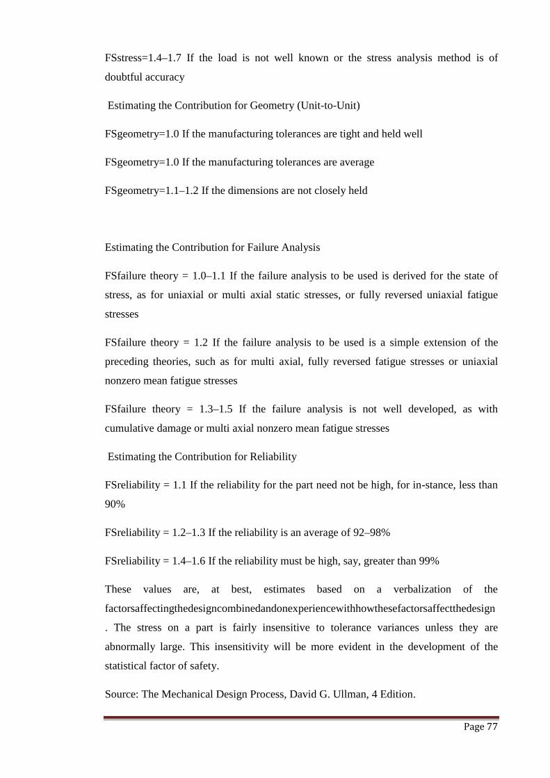
Page 77
FSstress=1.4–1.7 If the load is not well known or the stress analysis method is of
doubtful accuracy
Estimating the Contribution for Geometry (Unit-to-Unit)
FSgeometry=1.0 If the manufacturing tolerances are tight and held well
FSgeometry=1.0 If the manufacturing tolerances are average
FSgeometry=1.1–1.2 If the dimensions are not closely held
Estimating the Contribution for Failure Analysis
FSfailure theory = 1.0–1.1 If the failure analysis to be used is derived for the state of
stress, as for uniaxial or multi axial static stresses, or fully reversed uniaxial fatigue
stresses
FSfailure theory = 1.2 If the failure analysis to be used is a simple extension of the
preceding theories, such as for multi axial, fully reversed fatigue stresses or uniaxial
nonzero mean fatigue stresses
FSfailure theory = 1.3–1.5 If the failure analysis is not well developed, as with
cumulative damage or multi axial nonzero mean fatigue stresses
Estimating the Contribution for Reliability
FSreliability = 1.1 If the reliability for the part need not be high, for in-stance, less than
90%
FSreliability = 1.2–1.3 If the reliability is an average of 92–98%
FSreliability = 1.4–1.6 If the reliability must be high, say, greater than 99%
These values are, at best, estimates based on a verbalization of the
factorsaffectingthedesigncombinedandonexperiencewithhowthesefactorsaffectthedesign
. The stress on a part is fairly insensitive to tolerance variances unless they are
abnormally large. This insensitivity will be more evident in the development of the
statistical factor of safety.
Source: The Mechanical Design Process, David G. Ullman, 4 Edition.
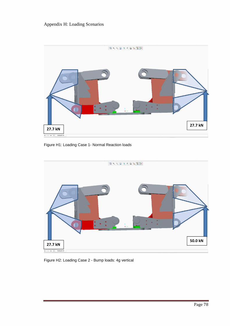
Page 78
Appendix H: Loading Scenarios
Figure H1: Loading Case 1- Normal Reaction loads
Figure H2: Loading Case 2 - Bump loads: 4g vertical
27.7 kN27.7 kN
27.7 kN50.0 kN
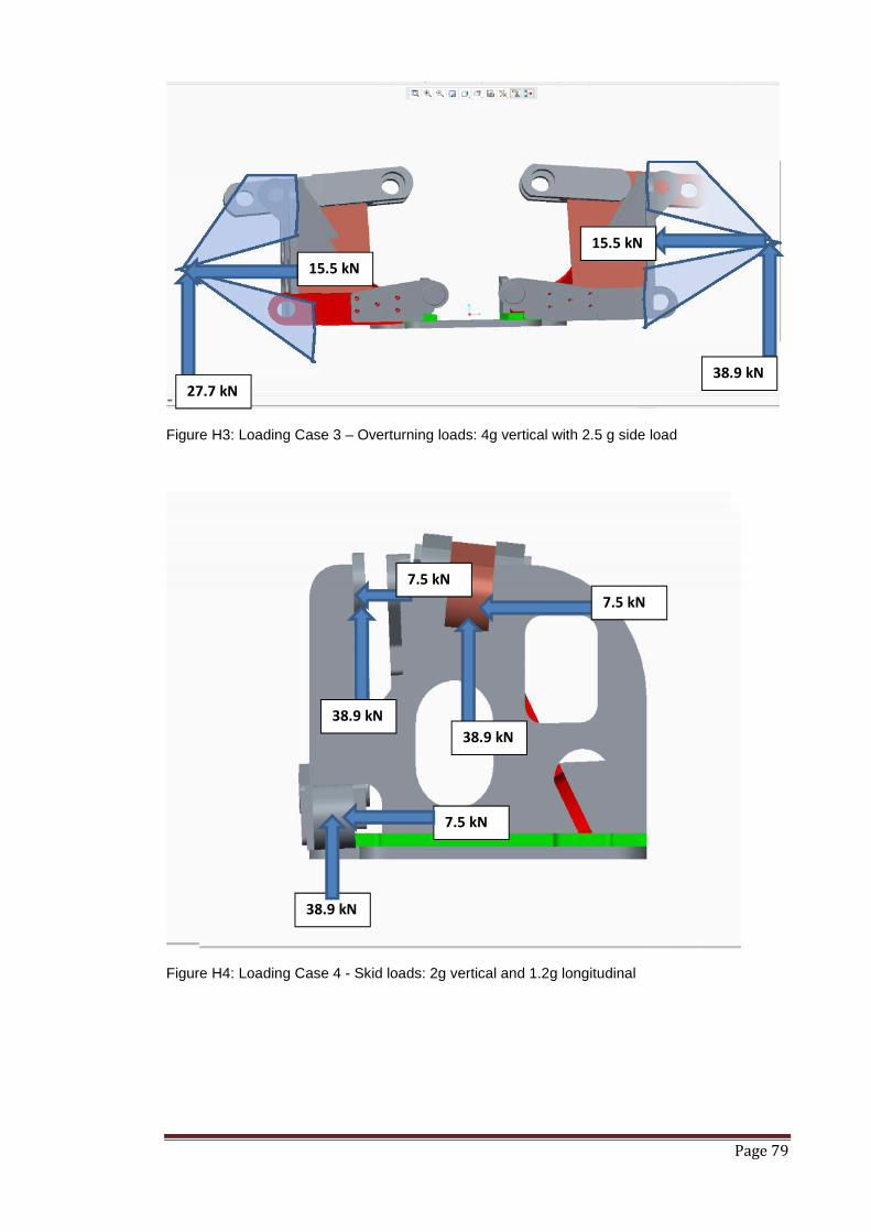
Page 79
Figure H3: Loading Case 3 – Overturning loads: 4g vertical with 2.5 g side load
Figure H4: Loading Case 4 - Skid loads: 2g vertical and 1.2g longitudinal
27.7 kN38.9 kN
38.9 kN
7.5 kN
15.5 kN15.5 kN
38.9 kN
7.5 kN
38.9 kN
7.5 kN
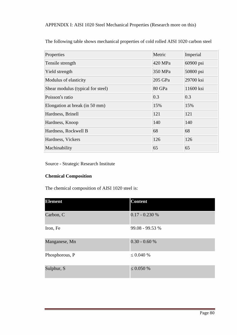
Page 80
APPENDIX I: AISI 1020 Steel Mechanical Properties (Research more on this)
The following table shows mechanical properties of cold rolled AISI 1020 carbon steel
Properties Metric Imperial
Tensile strength 420 MPa 60900 psi
Yield strength 350 MPa 50800 psi
Modulus of elasticity 205 GPa 29700 ksi
Shear modulus (typical for steel) 80 GPa 11600 ksi
Poisson’s ratio 0.3 0.3
Elongation at break (in 50 mm) 15% 15%
Hardness, Brinell 121 121
Hardness, Knoop 140 140
Hardness, Rockwell B 68 68
Hardness, Vickers 126 126
Machinability 65 65
Source - Strategic Research Institute
Chemical Composition
The chemical composition of AISI 1020 steel is:
Element Content
Carbon, C 0.17 - 0.230 %
Iron, Fe 99.08 - 99.53 %
Manganese, Mn 0.30 - 0.60 %
Phosphorous, P ≤ 0.040 %
Sulphur, S ≤ 0.050 %
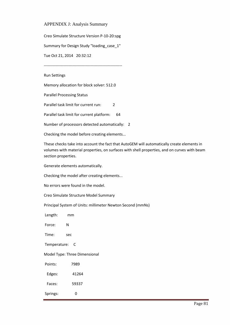
Page 81
APPENDIX J: Analysis Summary
Creo Simulate Structure Version P-10-20:spg
Summary for Design Study "loading_case_1"
Tue Oct 21, 2014 20:32:12
------------------------------------------------------------
Run Settings
Memory allocation for block solver: 512.0
Parallel Processing Status
Parallel task limit for current run: 2
Parallel task limit for current platform: 64
Number of processors detected automatically: 2
Checking the model before creating elements...
These checks take into account the fact that AutoGEM will automatically create elements involumes with material properties, on surfaces with shell properties, and on curves with beamsection properties.
Generate elements automatically.
Checking the model after creating elements...
No errors were found in the model.
Creo Simulate Structure Model Summary
Principal System of Units: millimeter Newton Second (mmNs)
Length: mm
Force: N
Time: sec
Temperature: C
Model Type: Three Dimensional
Points: 7989
Edges: 41264
Faces: 59337
Springs: 0

Page 82
Masses: 0
Beams: 0
Shells: 0
Solids: 26117
Elements: 26117
------------------------------------------------------------
Standard Design Study
Static Analysis "loading_case_1":
Convergence Method: Single-Pass Adaptive
Plotting Grid: 4
Convergence Loop Log: (20:32:43)
>> Pass 1 <<
Calculating Element Equations (20:32:44)
Total Number of Equations: 446124
Maximum Edge Order: 3
Solving Equations (20:33:06)
Post-Processing Solution (20:35:22)
Checking Convergence (20:35:44)
Resource Check (20:36:08)
Elapsed Time (sec): 237.23
CPU Time (sec): 158.64
Memory Usage (kb): 1113286
Wrk Dir Dsk Usage (kb): 1568768
>> Pass 2 <<
Calculating Element Equations (20:36:09)
Total Number of Equations: 492681
Maximum Edge Order: 7

Page 83
Solving Equations (20:37:45)
Post-Processing Solution (20:40:43)
Checking Convergence (20:41:19)
Calculating Disp and Stress Results (20:41:39)
RMS Stress Error Estimates:
Load Set Stress Error % of Max Prin Str
---------------- ------------ -----------------
LoadSet1 4.33e+00 1.6% of 2.64e+02
Resource Check (20:44:12)
Elapsed Time (sec): 721.47
CPU Time (sec): 356.51
Memory Usage (kb): 1157394
Wrk Dir Dsk Usage (kb): 1801216
Total Mass of Model: 6.340980e-01
Total Cost of Model: 0.000000e+00
Mass Moments of Inertia about WCS Origin:
Ixx: 1.91247e+05
Ixy: -5.01598e+03 Iyy: 9.59451e+04
Ixz: -1.91380e+04 Iyz: -9.14701e+03 Izz: 1.62265e+05
Principal MMOI and Principal Axes Relative to WCS Origin:

Page 84
Max Prin Mid Prin Min Prin
2.00763e+05 1.54603e+05 9.40912e+04
WCS X: 8.95835e-01 4.36877e-01 8.13523e-02
WCS Y: -4.09149e-03 -1.74950e-01 9.84569e-01
WCS Z: -4.44368e-01 8.82344e-01 1.54939e-01
Center of Mass Location Relative to WCS Origin:
( 1.29952e+02, 6.08340e+01, 2.37149e+02)
Mass Moments of Inertia about the Center of Mass:
Ixx: 1.53238e+05
Ixy: -3.13808e+00 Iyy: 4.95752e+04
Ixz: 4.03592e+02 Iyz: 9.58060e-01 Izz: 1.49210e+05
Principal MMOI and Principal Axes Relative to COM:
Max Prin Mid Prin Min Prin
1.53278e+05 1.49170e+05 4.95752e+04
WCS X: 9.95115e-01 -9.87206e-02 3.03099e-05
WCS Y: -2.92004e-05 1.26831e-05 1.00000e+00
WCS Z: 9.87206e-02 9.95115e-01 -9.73848e-06
Constraint Set: ConstraintSet1: BASEPLATE_SUBASSEMBLY
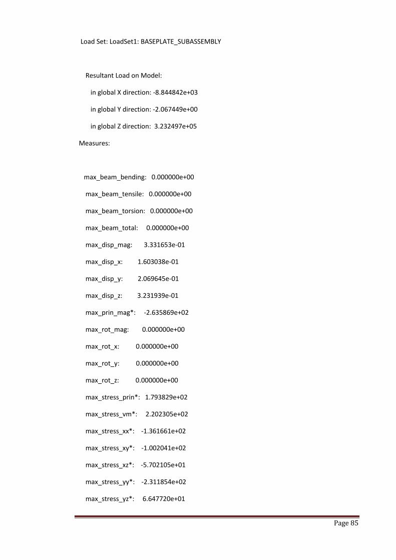
Page 85
Load Set: LoadSet1: BASEPLATE_SUBASSEMBLY
Resultant Load on Model:
in global X direction: -8.844842e+03
in global Y direction: -2.067449e+00
in global Z direction: 3.232497e+05
Measures:
max_beam_bending: 0.000000e+00
max_beam_tensile: 0.000000e+00
max_beam_torsion: 0.000000e+00
max_beam_total: 0.000000e+00
max_disp_mag: 3.331653e-01
max_disp_x: 1.603038e-01
max_disp_y: 2.069645e-01
max_disp_z: 3.231939e-01
max_prin_mag*: -2.635869e+02
max_rot_mag: 0.000000e+00
max_rot_x: 0.000000e+00
max_rot_y: 0.000000e+00
max_rot_z: 0.000000e+00
max_stress_prin*: 1.793829e+02
max_stress_vm*: 2.202305e+02
max_stress_xx*: -1.361661e+02
max_stress_xy*: -1.002041e+02
max_stress_xz*: -5.702105e+01
max_stress_yy*: -2.311854e+02
max_stress_yz*: 6.647720e+01

Page 86
max_stress_zz*: -1.399856e+02
min_stress_prin*: -2.635869e+02
strain_energy: 3.404424e+04
** Warning: The measures marked by an asterisk (*) were evaluated
at (or close to) results singularities. The values of these
measures may be inaccurate, and you must use engineering judgment
when interpreting them.
Analysis "loading_case_1" Completed (20:44:14)
------------------------------------------------------------
Memory and Disk Usage:
Machine Type: Windows Vista Service Pack 2
RAM Allocation for Solver (megabytes): 512.0
Total Elapsed Time (seconds): 734.99
Total CPU Time (seconds): 357.80
Maximum Memory Usage (kilobytes): 1168864
Working Directory Disk Usage (kilobytes): 1801216
Results Directory Size (kilobytes):
242106 .\loading_case_1
Maximum Data Base Working File Sizes (kilobytes):
1048576 .\loading_case_1.tmp\kblk1.bas
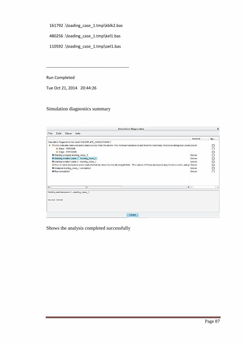
Page 87
161792 .\loading_case_1.tmp\kblk2.bas
480256 .\loading_case_1.tmp\kel1.bas
110592 .\loading_case_1.tmp\oel1.bas
------------------------------------------------------------
Run Completed
Tue Oct 21, 2014 20:44:26
Simulation diagnostics summary
Shows the analysis completed successfully

Page 88
APPENDIX K: Bill of Materials
Figure L1: Model exploded view
Part Number Name in Model Quantity1 PRT0021 22 PRT0001 23 PRT0007 24 BOLT 165 PRT0013 16 PRT0012 17 BOLT 108 PRT0024 19 LOWER_FRONT_PIN 210 PRT0026 111 BOLT 1012 PRT0017 113 PRT0009 114 25MM_PLATE3_MAI_SIDE_UPRIGHT 115 25MM_PLATE3_MAI_SIDE_UPRIGHTL 116 PRT0011RIGHT 117 PRT0016 118 PRT0011 119 PRT0015 1
1
32
4
25526
6 57
89
10
1423
21
192418
17
13
16
12
8
12
209
22
15
12
3
11

Page 89
20 PRT0026R 121 PRT0020 122 RIGHT_PLATE 123 PRT0010 124 RIGHT_FLANGE 125 PRT13_RIGHT 126 LEFT_LONG_BRACKET 127 CAR SCREW 16
Table L1: Bill of Materials

Page 90
Appendix L: Finite Element Analysis Software Comparison.
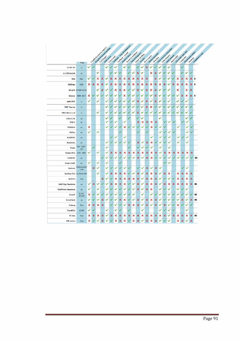
Page 91