INFOR1\fATION TO USERS

This manuscript has been reproduced from the microfilm master. UMI

films the text directly from the original or copy submitted. Thus, some

thesis and dissertation copies are in typewriter face, while others may

be from any type of computer printer.

The quality of this reproduction is dependent upon the quality of thecopy submitted. Broken or indistinct print, colored or poor quality

illustrations and photographs, print bleedthrough, substandard margins,

and improper alignment can adverselyaffect reproduction.

In the unlikely event that the author did not send UMI a complete

manuscript and there are missing pages, these will be noted. Also, if

unauthorized copyrightmaterial had to be removed, a note will indicate

the deletion.

Oversize materials (e.g., maps, drawings, charts) are reproduced by

sectioning the original, beginning at the upper left-hand corner and

continuing from left to right in equal sections with smaIl overlaps. Each

original is also photographed in one exposure and is included in

reduced form at the back of the book.

Photographs included in the original manuscript have been reproduced

xerographically in this copy. Higher quality 6" x 9" black and white

photographic prints are available for any photographs or illustrations

appearing in this copy for an additional charge. Contact UMI directly

to order.

V·M·IUniversity Microfilms International

A Bell & Howell Information Company300 North Zeeb Road. Ann Arbor. M148106-1346 USA

313/761-4700 800/521-0600

Order Number 9416063

Range determination from translational motion blur

Makkad, SatwinderpaI Singh, Ph.D.

University of Hawaii, 1993

V·M·I300 N. Zceb Rd.Ann Arbor, MI48106

RANGE DETERMINATION FROM TRANSLATIONAL MOTION BLUR

A DISSERTATION SUBMITTED TO THE GRADUATE DIVISION OF THE

UNIVERSITY OF HAWAII IN PARTIAL FULFILLMENT OF THE

REQUIREMENTS FOR THE DEGREE OF

DOCTOR OF PHILOSOPHY

IN

MECHANICAL ENGINEERING

DECEMBER 1993

By

SatwinderpalMakkad

Dissertation Committee

Joel S Fox, Chairperson

Ronald H. Knapp

Willem Stuiver

Ping Cheng

Wesley Peterson

ACKNOWLEDGMENTS

I would like to thank Professor Joel Fox for his help and invaluable guidance

during the course of this research. His intuitive explanations of complex problems

made them look easy. During a course on finite element analysis and my teaching

assistantship in his senior level design project class, Professor Ronald Knapp shared

his profound knowledge and insight into the practical aspects of design. I learned

from Professor Willem Stuiver the importance of consistent effort to solve ill-defined

problems in his optimization class. Professor Wesley Peterson's encouragement and

knowledge of Fourier analysis is gratefully acknowledged. I learned numerical

methods and analysis from Professor Ping Cheng and I thank him for serving on my

dissertation committee. I am very grateful to Professor Richard Fand for his counsel

upon matriculation into the university.

I am fortunate to have had the support of so many good friends. We together

shared our hopes and dreams. I thank them all for being my family away from home.

I am very grateful to all members of my family: my Mom, Dad, and my

brothers Mintoo and Sitoo for their strength and unconditional support in my

endeavors. I dedicate this dissertation to them.

iii

ABSTRACT

A survey is carried out and the principles of various range sensing techniques

are described. A method to determine range from a translationally blurred and a sharp

image is presented. To decode the length of blur in the translationally blurred image,

three decoding methods; minimization approach, Fourier transform approach, and

method-of-slopes, were tested on various images. The results were found to be

favorable for the minimization approach and the method-of-slopes. Ringing was

encountered with the Fourier transform approach. The minimization approach is

iterative and slow. The method-of-slopes was investigated further for the case of

inclined plane surfaces and the results were found to be favorable. The method-of­

slopes can also determine disparity for cylindrical surfaces. A rotating mirror system

is described, which simulates camera translation in order to produce a linearly blurred

image, in real-time.

iv

TABLE OF CONTENTS

ACKNOWLEDGMENTS . .iii

ABSTRACT . .IV

TABLE OF CONTENETS .. .V

LIST OF FIGURES .vii

CHAPTER 1 MACHINE VISION AND RANGING TECHNIQUES . .1

1.1 Introduction .. .1

1.2 Range Determination .2

1.3 Active Ranging Techniques .3

1.3.1 Time of Flight: Laser Range Finders . .3

1.3.2 Triangulation .. . .5

1.3.3 Interferometric Techniques . . .7

1.3.3.1 Moire Technique. .8

1.3.3.2 Holographic Technique. .10

1.3.4 Focusing .. .12

1.3.5 Fresnel Diffraction .12

1.4 Passive Ranging . .15

1.4.1 Structure from Motion of Camera . .16

1.4.2 Structure from Optical Flow . .17

1.4.3 Shape from Shading and Photometric Stereo. .18

1.4.4 Shape from Texture . .22

1.4.5 Stereopsis .. .25

1.4.6 Range from Defocus .. .28

CHAPTER 2 TRANSLATIONAL BLUR, GENERATION AND

DECODING .31

2.1 Introduction .. .31v

2.2 A model for translational blur .32

2.2.1 Spatio Temporal Point of View . .35

2.2.2 Optics for Blur Generation .. .38

2.3 Decoding Methods . .40

2.3.1 Minimization Approach .. .42

2.3.2 Fourier Transform Approach . . .43

2.3.3 Method of Slopes ., . . .44

CHAPTER 3 TESTS FOR ROBUSTNESS, SIMULATION AND REAL

IMAGE ANALYSIS. . .47.

3.1 Introduction.. . .47

3.2 Tests for Simulated Rectangle Function Images. .47

3.3 Results Using Quasi-Real Images . .50

3.4 Blur Images From Rotating Mirror .. .54

3.5 Analysis .. . . . . . . . . .54

CHAPTER 4 EXPERIMENTS, METHOD OF SLOPES .59

4.1 Introduction. . . . . .59

4.2 Inclined Plane Surface . .59

4.3 Simulation and Analysis: Isoplanatic Approach .. .66

4.4 Simulation and Analysis: Intensity Division Approach. . .72

4.4.1 Inclined Plane. . .

4.4.2 Cylindrical Surface .

4.4.3 Quasi-Real Images ..

CHAPTER 5 CONCLUSION.

5.1 Summary.

5.2 Assumptions and Limitations ..

5.3 Future Work

REFERENCESvi

.78

.78

.92

.97

.97

.98

.98

.99

LISTOF FIGURES

FIGURE

1.1 A triangulation based range finding geometry

1.2 Principle of Moire technique.

1.3 Principle of focusing method .

1.4 Fresnel diffraction .

1.5 A surface patch configuration

1.6 Surface gradient components.

1.7 Surface orientation components .

PAGE

.6

.9

.13

.14

.19

.21

.23

1.8 An orientation geometry for an orthogonal texture pattern. .24

1.9 A schematic of stereo imaging system. .26

2.1 Disparity for a stereo pair and a blur image. .33

2.2 Geometry for translational blur. .34

2.3 A stack of successive images. .36

2.4 Integration of brightness in a spatio-temporal plane .37

2.5 Principle of the displacement of optical axis. .39

2.6 A schematic of image formation system . .41

2.7 An edge separating two regions of linearly varying brightness .46

3.1 Stationary image.

3.2 Blurred image.

3.3 Blurred image with a pixel noise (10% of the max.) .

3.4 Point Spread Function (Fourier transform approach) .

3.5 Quasi-real images. . .

3.6 Results of minimization approach for quasi-real images.vii

.48

.49

.51

.52

.53

.55

.56

.57

.60

.65

.67

..68

3.7 Schematic of the experimental setup

3.8 Real images . .

4.1 Imaging of a plane surface inclined to the optical axis

4.2 Blur-acute pair

4.3 A blur-acute pair with variable brightness gradient

4.4 Disparity of isoplanatic surface patches with variable brightness

gradient.. . . .. . .

4.5 A blur-acute pair with different brightness levels, a constant

brightness gradient, and a gradient in disparity. .69

4.6 Results of blur-acute image pair with a gradient in disparity .70

4.7 A blur acute pair for surfaces with different gradients in disparity .71

4.8 Results for surfaces with three different disparity gradients .73

4.9 A blur-acute image set for a scene consisting of three isoplanatic

.74

.75

surfaces with different disparity and brightness levels

4.10 Disparity for three isoplanatic surfaces .

4.11 Results of intensity-division approach using left acute and blurred

images .. . . .76

4.12 Results of intensity-division approach using right acute and blurred

images . . . . . . . . . . . . . . . . . . . . . .77

4.13 A blur-acute image set for three inclined plane surfaces with different

.79

.. 81

.80

brightness gradients. . . .

4.14 Three inclined plane surfaces.

4.15 Results for three inclined plane surfaces

4.16 A blur-acute image set for three inclined plane surfaces with the

Gaussian noise of the order of 1% of the maximum gray level .82

4.17 Results of blur-acute image set with 1% Gaussian noise. .83viii

4.18 Results of blur-acute image set with 5 % Gaussian noise. .84

4.19 Two inclined planes and a semi-cylindrical surface . . .85

4.20 A blur-acute image set for two inclined planes and a semi-cylindrical

surface . . . . . . . . . . . . . . . . . . . . . .86

4.21 Results of inclined plane and semi-cylindrical surface (included angle

of the semi-cylindrical surface = 180°) . . . . . . . . . . .87

4.22 Results of inclined plane and semi-cylindrical surface (included angle

of the semi-cylindrical surface = 175°) . . . . . . . . . . .88

4.23 Results of inclined plane and semi-cylindrical surface (included angle

of the semi-cylindrical surface = 170°) . . . . . . . . . . .89

4.24 A blur-acute image set for two inclined planes and a semi-cylindrical

surface with 1% Gaussian noise. . . . . . . . . . . . . .90

4.25 Results of inclined planes and a semi-cylindrical surface in presence of

1% Gaussian noise . . . . . . . . . . . . . . . . . .91

4.26 A blur-acute image set for two inclined planes and a semi-cylindrical

surface with 5 % Gaussian noise. . . . . . . . . . . . . .93

4.27 Results of inclined planes and a semi-cylindrical surface in presence of

5 % Gaussian noise . . . . . . . . . . . . . .94

4.28 A quasi-real blur-acute image pair of a cylindrical object .95

4.29 Results of quasi-real images of a cylindrical object . . .96

ix

CHAPTER 1.

Machine Vision and Ranging Techniques

1.1 Introduction

Needs for faster and accurate systems dictate a move towards automation.

Automation of any process or machine operation requires various sensory inputs. One

of these input can be visual input. Some applications needing visual information can

be structured, as in case of an inspection and manufacturing process, or non­

structured, as in case of guarding a compound from intruders, navigating around a

course filled with obstacles. In a structured environment where surrounding factors

such as illumination and work place arrangement can be controlled, the visual

information needed may be two dimensional, for example; the size of a part from its

geometry, or the orientation of the part based on its configuration. Three dimensional

information is required, however, in a non-structured environment where the

surroundings can be controlled only to some extent or cannot be controlled at all.

Three dimensional information helps in approaching an object, in handling,

determining the size of the object, navigation.

Three dimensional information can be acquired by various range sensors. The

range sensors used today vary in type and nature depending on their application. The

range sensors based on imaging use a camera which collapses the three dimensional

information about a scene into two dimensional image format. One of the functions of

a machine vision system is to extract desired three dimensional information from these

two dimensional images.

1.2 Range Determination

Range determination is a very basic, yet a difficult problem. In order to

understand a visual scene realistically, the three dimensional structure of the scene

must be known. This information can be used in many industrial applications

including automatic inspection of manufactured parts, autonomous vehicle guidance

[Thorpe, 1990], robotic manipulation [Fairhurst, 1988], and automatic assembly.

Range information is a collection of distance measurements, made from a

reference plane or coordinate system to the surface points on objects in a scene [Besl,

1988]. A range imaging device is defined as any combination of hardware and

software capable of producing a range image of a real world scene under appropriate

operating conditions. Range images, depending on context, are known by many

names: range map, depth map, depth image, range picture, rangepic, 3-D image, 2.5­

D image, digital terrain map (DTM), topographic map, 2.5-D primal sketch, surface

profiles, xyz point list, contour map, surface height map, etc.

A few surveys of range imaging methods were carried out in the early eighties

[Kanade and Asada, 1981, Strand, 1984, 85], and Jarvis[1983] presented a more

elaborate survey from the optics point of view. Since then, a few additional surveys

have been carried out [Kale, 1985, Svetkoff, 1986, Wagner, 1987]. In his exhaustive

survey, Besl [1988] gave quantitative performance comparisons between different

active optical range sensing methods.

All the range finding methods available today can be subdivided into two

categories: active ranging and passive ranging.

2

1.3 Active Ranging Techniques

In active ranging a controlled beam of energy is radiated into the field of view

and the returned radiation response is then analyzed to determine the range.

According to Besl [1988], most active optical techniques for obtaining range images

are based on one of the five principles: (1) time of flight, (2) triangulation, (3) Moire

and holographic interferometry, (4) lens focus and, (5) fresnel diffraction. Here,

using suitable examples, the basic principles of each of these techniques are presented.

1.3.1 Time of Flight: Laser Range Finders

Time-of-flight laser range finders are based on the principle of a signal

traveling from a source, to an object, and back to receiver. Assuming the source and

the receiver are coplanar, the basic equation for such a system is:

v,Z=-

2(1.1)

where z is range, v is the speed of signal propagation, and 't is the transit time from

source to object and back to the receiver. Time-of-flight detectors provide the

absolute range data directly. No image analysis is required.

Time-of-flight can be determined by: (1) pulse modulation, (2) amplitude

modulation, or (3) frequency modulation. In pulse modulation based range finders a

pulsed laser is emitted by the source and the returned signal is scanned for the pulse.

The time difference results in range information. An imaging laser radar [Lewis and

Johnson, 1977] for a mobile robot was built on the pulse detection principle. The

3

accuracy of the range finder was of the order of 2.0 em over a range of 1 to 3 meters.

A superior sensor was built by Jarvis [1983a], which could acquire a range image

containing 64x64 pixels in 4 seconds.

Instead of pulsating, the laser can be amplitude modulated [Sanz, 1989]. This

eliminates the wait time for an echo, as in the case of a pulsed signal, as the

amplitude of the returning signal can be compared to the emitted signal at any

moment to check for the phase shift. This measured phase shift provides the range

il.wz=_·!J.¢

47f(1.2)

where A.AM is pulse wave length, !J.lj> is the phase shift. One of the first non-military

radar was built by Nitzan et al [1977].

The laser can also be frequency modulated [Sanz, 1989]. By repetitively

sweeping the optical frequency (between v±!J.v), a total frequency deviation of !J.v is2

created during the period )t where j. is the linear sweep modulation frequency.

The returned signal can be mixed coherently with a reference signal at the detector, to

create a beat frequency signal (fi) which depends on the range z of the object. This

detection process is known as FM coherent heterodyne detection,

cfiz=_..=c.--4 j.!J.v

4

(1.3)

where c is some constant of proportionality. Beheim and Fritsch [1986] have

constructed a range finding device which can measure a range of 1.5 meter with

subcentimeter resolution.

1.3.2 Triangulation

The simplest, most obvious, and most commonly used range finding concept is

triangulation. It is based on the law of sines:

sin(A) ex: asin(A) _ sin(B) _ sinCe)

or - --~

abc(1.4)

If a camera is aligned along the z-axis (Fig. 1.1), and a beam of light from a

projector at a distance of x, (inclined by an angle 8 with respect to z-axis) is projected

onto the scene, then the range z of the point P on any object surface is given by the

relation:

z =x- tan(B) (1.5)

The survey can be subdivided into ranging methods based upon the geometry

of the projected of light: (1) point light, (2) line light, (3) coded binary pattern, and

(4) color coded stripes of light. Bicknel et al.[1985] described a method of building a

triangulation based system using spot ranging. This system can achieve a resolution of

25~m, over a depth of field of 100 mm, at a range of 500 mm. Begin [1988] used a

spot ranger for welding application. The resolution of the ranging device was of the

order of 0.65 mm for a range of 1000 mm. Hausler and Maul [1985] reported a

telecentric scanner configuration for ranging objects with a diameter 1 m. or less,

with a ranging resolution of == 0.1 mm. Faugeras and Hebert [1986] used a spot laser

5

p

z

o

Projector

"

Fig 1.1 A triangulation based range finding geometry

6

Camera

range finder based on triangulation. The object is placed on a rotating turn table and

is detected by two horizontal position sensors, and scans are taken by changing the

elevation of the laser spot. A spot ranger measures single point per sampling interval.

Shirai [1972], and Nevita and Binford [1973] used a range finder based on light

stripes to range objects containing planer surfaces. Fewer sampling frames are

required as all the points in a line stripe can be ranged simultaneously. PoppIestone et

al [1975] furthered the light stripe method to incorporate the ranging of curved

surface objects. All the above light stripping methods were intended to build an

algorithm for the recognition of a three dimensional object. A sensor for industrial

application was built by Ozeki et al [1986]. It could range an object in a 60 ern square

area at a distance of 100 em at 48x50 point with an accuracy of ±2 em. Sato et al

[1982] used a double slit projector to further the single stripe concept. Their test

results show an accuracy of 0.5 mm over a range of the order of 1030 mm. Jaliko et

al [1985] reported a multistripe system design using 16 vertical stripes. Stripes are

shifted laterally in 8 consecutive frames to produce a horizontal resolution of 128

pixels. Potmesil [1983] reported using a grid of orthogonal isoparametric projected

lines. Altschuler et al [1981] described a spot coded laser beam patterns for ranging,

and Boyer and Kak [1987] used a color encoded structure of light stripes in which

only one image frame is required.

1.3.3 Interferometric Techniques

Interferometric techniques can be subdivided into (1) Moire and, (2)

holographic interferometry.

7

1.3.3.1 Moire Technique

When one amplitude modulated spatial signal (reflected light from a scene) is

multiplied by another amplitude modulated spatial signal (viewing grating) the

resulting interference phenomenon can be given by [Sanz, 1989]:

where Ai represent amplitudes, mi are the modulation indices of amplitude

modulation, coi the spatial frequencies, and <l>i the slowly varying phases. When this

signal is low pass filtered (blurred) with a cut off frequency below the minimum of co

I and co2, only the frequency difference terms and constants are carried through,

resulting in

For equal spatial frequencies only the phase difference terms are left

LPF{A(x)} =A.A2{(1 +m.m2. cos(~(x) - 9h(x»}

(1.7)

(1.8)

Range information is contained in these phase difference terms. In a simple

experimental setup (Fig. 1.2) a Moire fringe interference pattern is formed by

illuminating a scene with shadow pattern, using a uniformly spaced optical grating,

and viewing the scene through an identical grating placed in front of a camera. The

projector is displaced laterally from the camera.

8

L Object surface

Light

Image plane

Fig. 1.2 Principle of Moire technique

9

A detailed survey can be found in Besl [1988]. Moire range imaging methods

are used for measuring the relative distance between surface points on a smooth

surface with no discontinuities. Cline et al [1982, 84] have reported some

experimental results, and Gasvik [1983] addressed the limitations of the projection

Moire method.

1.3.3.2 Holographic Technique

In holographic interferometry, two coherent beams of light from a light source

are used to produce interference patterns, due to the optical frequency phase

differences, in different optical paths. If two laser beams meet at a surface point, then

the two beams add up to produce a net electric field given by [Bes1, 1988]:

where ei are electric field intensities, Ki are the wave vectors, Wi are the optical

frequencies of light beams, and ~i are the phases. Detectors of light respond to the

intensity of radiation (the square of electric fields). Here, intensity (irradiance) is

given by:

1( - t) - 2 - 2x, =el +e2 (1.10)

When the equation is expanded and low pass filtered in terms of optical

10

(1.11)

where .1co = co rco2, .1K = K1-K2' .1<1> = 4>1-4>2' This is similar to equation (1.7)

except that vector variations have been explicitly used for wave vectors (vector spatial

frequencies). For the same optical frequencies and equal vector spatial frequencies,

only the phase difference term remains. It is these phase difference terms that carry

surface depth information. Similar to Moire technique the holographic interferometry

is used for measuring the relative distance between surface points on a smooth surface

with no discontinuities.

The first evidence of holography can be found in Leith and Upatnieks [1962].

Church et at [1985] describe the industrial uses of holography, and Tozer et al [1985]

have reported the application of holography for measuring the fuel element size in a

nuclear reactor. Wuerker and Hill [1985] have used holography for recording the dust

particle phenomenon. They have achieved a resolution on the order of 2-4 urn over

the conventional microscopes resolution of 10-100 urn, Pryputniewicz [1985] used

heterodyne hologram interferometry to study the load deformation characteristics of

computer micro components which were surface mounted on a printed circuit board.

Thalmann and Dandliker [1985] discussed the application of heterodyne and quasi

heterodyne (stepwise phase shifting) fringe interpolation techniques for contouring of

3-D object shapes, and Dandliker and Thalmann [1985] discussed the possibility of

automating the interferogram processing. Hariharan [1985] described a technique to

use a television camera to compute the range of points on a surface.

11

1.3.4 Focusing

The simple lens formula is given by the equation:

1 1 I-=-+-f z v

(1.12)

The principle of this method is based on the distance of the image plane from the

focal plane in a camera. If the object is at an infinite distance, the image forms at the

focal plane (Fig. 1.3) of the lens. If the object is closer to the lens, the image is

formed at the image plane, which is away from the focal plane. The distance of the

image plane from the focal plane can be calibrated in terms of object range. The

camera instruments can also be calibrated in terms of focus sharpness of the objects

on the image plane and Jarvis [1983] has suggested some focus sharpness measures.

Results of some other surveys will be discussed later, in section 1.4.6 (range from

defocus).

1.3.5 Fresnel Diffraction

If an aperture is illuminated by a plane wave (light), and the fresnel diffraction

is formed on a plane on unknown distance away, then the size and shape of the

diffraction pattern can be used to determine the distance between the aperture and the

image plane. This principle has been extended to measure absolute distance and to

determine the depth of 3-D objects. The general description of a fresnel phenomenon

can be found in any physical optics book [Jenkins and White, 1937]. A simple optical

setup [Leger and Snyder, 1984] based on this principle is shown in Fig. 1.4. This

12

'- v~~_1mm

f-f-j

..................................................... ········HE·································!Focal plane;

j

"0

.-._.-._.... -. _.-.-._._. _. _. -._. -._._._. ~. _.-.;

" I

,;

iImageplane

i" z--I- i v ", J::::...::__~.__._._._._-._._._._-._._._._-._._._.-__ ._._-_._._.r_-n..~~.m~ r

a =r-- I ' i

r = blur circle radius

a = apertureof the lens

z = distance of a point

v = image-plane distance

Fig. 1.3 Principle of focusing method

13

Coherentplane oflight

Grating

Half mirrored surface

Processor

Fig. 1.4 Fresnel diffraction

14

3-dimensionalinformation

setup is based on the Talbot effect, which refers to the self imaging property of a

grating [Winthrop and Worthington, 1965]. According to this effect, any amplitude

distribution which is a periodic function of x and y will also be periodic in the

direction of propagation z. In this setup, a coherent beam of light is projected through

a simple periodic cosine grating aligned vertically (along y-axis). If a screen is placed

at a distance z from the grating, the intensity on screen will have a periodic

modulation whose fundamental frequency is equal to that of the grating. If a contrast

ratio is defined as the ratio of power in the fundamental frequency to the power in the

zero frequency component, then this contrast ratio is a function of the distance

between the screen and the grating. Since this technique measures fringe contrast this

approach is insensitive to the reflectance variations in the object. Chavel and Strand

[1984] have reported some experimental results for 512x512 pixel images. No

accuracy figure was available.

Some of the disadvantages of active ranging are: (1) probing instruments are

power intensive, (2) the need for high energy probing beams precludes their use in

presence of humans, (3) in military applications because of the need to emit a beam of

radiation the stealth of the user is compromised.

1.4 Passive Ranging

Human vision is the inspiration behind nearly all the passive ranging

techniques. Depth cues used by human eye have resulted in various passive ranging

techniques. They can be classified into the following categories: (1) structure from

motion, (2) structure from optical flow, (3) shape from shading and photometric

stereo, (4) shape from texture, (5) stereopsis and, (6) range from defocus.

15

1.4.1 Structure from Motion of Camera

The structure-from-motion approach is based on two steps: (1) compute the

observables in the image, and (2) relate these to structure in the space. The

observables can be points, lines, contours etc. The observation of a number of points

in two or more views can yield the position of these points in space and the relative

displacement between the viewing systems. Roach and Aggarwal [1979, 1980] used

the basic equation that relates the 2-D projection (x,y) to a 3-D point (x,y,z):

x = f all(x-xO)+aI2(Y- yo)+al3(z-zo)a3{x- xo) +a32(Y - yo) +a33(z-zO)

(1.13)

(1.14)

where (xo,yo,zo) are the 3-D coordinates of the lens center and all' a12, a13, ~I' ••• ,

a33 are functions of camera orientation in a global coordinate system. Researchers

have tried to solve this equation by different approaches. Roach and Aggarwal

[1979,1980] took two views of a scene from two camera positions. They needed five

points in order to solve one set of the equation. Webb and Aggarwal [1982] used

multiple images with a single camera view to recover the 3-D structure of moving

rigid and jointed objects. Matthies et al [1988] reported a pixel based algorithm using

Kalman filtering, in which the depth estimate and depth uncertainty at each pixel is

incrementally refined over time using a sequence of images obtained with known

motion of the camera in robot navigation.

16

1.4.2 Structure from Optical Flow

Prazdny [1980] described the possibility of using the optical flow information

created on retina of a moving observer to derive a relative depth map. Optical flow is

the field of instantaneous apparent velocities of points on the surface of objects

moving in space. It is the apparent motion of the brightness pattern [Hom, 1986].

Optical flow can also be defined by the instantaneous distribution of the angular

velocity as of the projection ray passing through an object point P [Sanz, 1989]. The

angular velocity consists of two components, a translational component at, and a

rotational component ar.

(1.15)

For a moving object, the rotational velocity does not vary from point to point on the

object surface. The translational component changes due to the distance from point to

the projection center, given by

T·Pa.=ar+--

sin( 77)and

T·sin(77)OJ = __0...=-

S(1.16)

where T is the translation vector, P is the positional vector, T) is the angle between the

two vectors, and s is the distance between the object point P and the origin O. Even

though all the points on the object surface undergo the same translation T, the portion

of the translation which is perceived as the motion in the image depends on the

direction of the translation and the distance of the object point from origin. The

directional components perpendicular to the positional vector show up on the image

17

plane, and the velocity component parallel to the direction of projection vector are

lost in the process of image formation. Therefore the difference between the

translational component at of two points can be used to determine their relative

distance:

(1.17)

where PI and P2 are unit vectors in the direction of points PI and P2, aSI and aS2

represent the optical flow, and SI and S2 denote the distances of point PI and P2 from

the origin in 3-D coordinate system. A detailed review on optical flow is given in

Hom [1986], and Horn and Schunk [1981].

1.4.3 Shape from Shading and Photometric Stereo

This method is based on the concept of using image intensity information to

recover the surface orientation from one or multiple images. Shape from shading uses

one image and surface smoothness constraint, whereas photometric stereo uses several

views of an object, taken with varying illumination but the same viewing direction.

Let us consider a surface patch as shown in Fig. 1.5. If the viewing direction is

aligned to the z-axis, the shape of a 3-D object can then be described by its height

above the x-y plane. In terms of surface brightness one can write (Ballard and Brown

[1982])

z = - f(x,y)

18

(1.18)

Surface normal

Surface patch

~ tch configuration1 ,. A surrace paFig. .J

19

and the surface gradients can be defined as (Fig. 1.6)

8zp=­

&:and

8zq=-

OJ(1.19)

If we define a general plane equation as

Ax+Bx+Cz+D = 0

It can be expressed in terms of gradients as

A B D-z = -x + - Y + -

C C C

(1.20)

(1.21)

or -z = px + qy + k (1.22)

where A,B,C,D and, k are some constants. The two dimensional space of vectors

(p,q) is known as gradient space. A reflectance map R(p,q) is defined by associating

with each point (p,q) in gradient space the brightness of a surface patch with the

specified orientation, and is usually depicted by means of iso-brightness contours.

R(p,q) can be obtained experimentally using a test object or a sample mounted on a

galvanometer.

The reflectance map provides a simple constraint for recovering 3-D shape

from shading information. The constraint is expressed by the image irradiance

equation

R(p,q) = f(x,y)

20

(1.23)

y-axis """

' .... "~-----------------------IIIIIII

Fig. 1.6 Surface gradient components

21

x-axis

where (p,q) denotes the possible orientations at the point (x,y). Since one constraint is

not enough for determining a unique solution for (p,q), additional constraints are

required. As mentioned earlier, the shape from shading concept uses one view and

surface smoothness as additional constraint. The photometric stereo method uses

multiple images (generally 3 or more), with different lighting conditions and the same

viewing position.

Ikeuchi and Hom [1979] have implemented the photometric stereo method

using the reflectance map technique experimentally. Hom and Ikeuchi [1981] reported

experimental results for an iterative shape-from-shading algorithm using the

smoothness constraint for a synthesized lambertion sphere. The result show an error

of the order of 0.01 % after 30 iterations. Since photometric stereo can determine

surface information rapidly but can not determine absolute depth values, Ikeuchi

[1987] has reported a duel photometric stereo system to obtain absolute depth values.

It combines the photometric stereo with binocular stereo, and is called binocular

photometric stereo or duel photometric stereo.

1.4.4 Shape from Texture

A source of cue to surface orientation under perspective projection is texture.

Texture can be segmented into primitives. Under the assumption of planarity and

uniform distribution, the gradient of texture density provides surface orientation

information [Sanz, 1989]. A texture gradient can be described as the direction of

maximum rate of change of projected primitives size. The orientation of the texture

gradient vector corresponds to the tilt 0 s tl s 1800 with respect to camera axis and

the magnitude determines the slant 0 s sl s 900 (Fig. 1.7). For a regular texel texture

such as parallel lines from a rectangular grid under perspective projection (Fig. 1.8),

22

Tilt

y-axis

/Camera axis

Surface normal

Slant

x-axis

Fig. 1.7 Surface orientation components

23

y-axis

(-) x-axis

~Tilt

note: z-axis is perpendicular to the piece of paper

Fig 1.8 An orientation geometry for an orthogonal

texture pattern

24

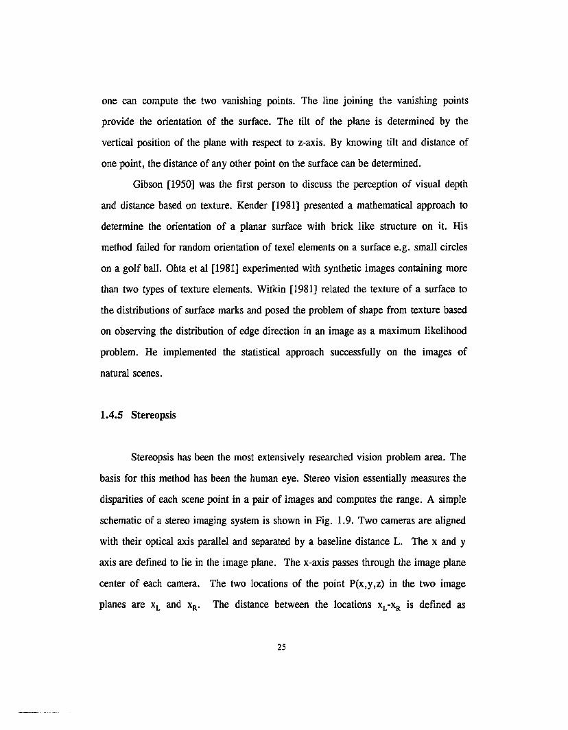
one can compute the two vanishing points. The line joining the vanishing points

provide the orientation of the surface. The tilt of the plane is determined by the

vertical position of the plane with respect to z-axis. By knowing tilt and distance of

one point, the distance of any other point on the surface can be determined.

Gibson [1950] was the first person to discuss the perception of visual depth

and distance based on texture. Kender [1981] presented a mathematical approach to

determine the orientation of a planar surface with brick like structure on it. His

method failed for random orientation of texel elements on a surface e.g. small circles

on a golf ball. Ohta et al [1981] experimented with synthetic images containing more

than two types of texture elements. Witkin [1981] related the texture of a surface to

the distributions of surface marks and posed the problem of shape from texture based

on observing the distribution of edge direction in an image as a maximum likelihood

problem. He implemented the statistical approach successfully on the images of

natural scenes.

1.4.5 Stereopsis

Stereopsis has been the most extensively researched vision problem area. The

basis for this method has been the human eye. Stereo vision essentially measures the

disparities of each scene point in a pair of images and computes the range. A simple

schematic of a stereo imaging system is shown in Fig. 1.9. Two cameras are aligned

with their optical axis parallel and separated by a baseline distance L. The x and y

axis are defined to lie in the image plane. The x-axis passes through the image plane

center of each camera. The two locations of the point P(x,y,z) in the two image

planes are XL and xR• The distance between the locations XL-xR is defined as

25

Pfx.y.z)

Image ---L.._--l-__

plane xL

r

z

f

L

I-------L-------i

Fig. 1.9 A schematic of stereo imaging system

26

disparity. By simple trigonometry, one can see that range of the point P can be given

by (note YL = YR):

fz =L--

XL-XR(1.24)

The main difficulty in any stereo system is in the so called "correspondence

problem", which consists of identifying corresponding points in the two images. This

problem arises because of several factors [Sanz, 1989]: (1) points of interests may

lack sufficient information to establish a unique pairing relationship in two images,

e.g. lack of intensity or color identifiers, (2) several candidate points may satisfy

matching criteria resulting in false identification, e.g. a planar surface containing a

regular pattern, (3) due to occlusion effects some parts may appear in one view but

not in the other, e.g. vertical facets parallel to the camera axis. This effect can be

reduced by reducing the separation distance L which in tum reduces the range

accuracy.

The main objective of any stereo system is to select some type of features and

a matching criteria. Features can be low level e.g. dots, edges, local texture, which

are relatively easy to detect but are difficult to match. High level features e.g.

specific object shape, are difficult to detect, but once selected they are easy to match.

Julesz [1964] presented experimental results based on random dot stereograms. His

work demonstrated that human vision is capable of interfering depth even in the

absence of high level clues for disparity. This observation provides a basis for stereo

vision based on low level primitive features. Some researchers select a small area in

one image and carry out cross correlation with similar size area in the other image

[Bernard and Thompson, 1980]. Moravec [1979, 1980] tested a rover robot which

27

used 9 stereo pairs along a base line for mapping surroundings, based upon area

matching technique to find disparity. The robot took 10-15 minutes to travel a

distance of 1 meter. Weissman [1980] described a stereoscopic system which acquires

a stereo image pair, aligns and enhances the images. Feature selection and matching

is accomplished manually. Marr, Poggio and Grimson [1985] carried out matching of

edges detected by zero-crossing, obtained by using a DOG (difference of Gaussian)

like operator called primal sketch operator (Laplacian of Gaussian). Grimson also

discusses the reconstruction of shapes from edges for matching purpose. Leung and

Huang [1990] reported detection of wheels of vehicles in stereo images.

1.4.6 Range from Defocus

In any imaging system, the objects falling within the depth-of-focus are

sharply focused on the image plane, while the objects closer than and away from the

depth-of-focus are blurred or defocused on the image plane. The amount of defocus is

a function of depth, and Pentland [1985,1987] used this concept to derive a depth

map. A thin lens follows the lens Eq. (1.12). It can also be written in alternative form

as:

z = ..l.!-v-f

(1.25)

For a closest point at distance Zo the focused image plane distance is Va (Fig. 1.3). If

the image plane is fixed at this location, then for any point at a distance Z> Zo the

image results in a blur circle of radius r. From simple geometry one can see that

a rtan(U) = =

v vo-v28

(1.26)

i.e. v =a v.

v.+a(1.27)

where a is the aperture of the lens. Substituting Eq. (1.27) into (1.25) gives:

1 v.

v.-1(1+1~)(1.28)

By measuring the amount of blur given by blur circle radius r, the range z of the

corresponding point in the scene can be determined.

Subbarao [1987] described three methods to recover the range. These methods

are based on measuring the change in an image due to a small known change in one of

the three intrinsic camera parameters: (1) distance between the image detector plane

and the lens, (2) focal length of the lens, and (3) diameter of the lens aperture.

Subbarao and Gurumoorthy [1988] derived a closed form solution for a step

discontinuity. Grossman [1987] reported some experiments using 512x512 images.

The accuracy of results vary from 10% to 50 %, based on the averaging window size.

The experimental results presented by Krotkov and Martin [1986] have a magnitude

of error on the order of 10% of the object distance between 1 and 2 meters. Trevor

and Wohn [1988] presented a method of depth recovery through the analysis of scene

sharpness across a changing focus position. The performance of the range finder was

limited by the time it took focus and to zoom motors to move through all the sample

focus positions. A depth map with 10 levels of depth resolution took 10 seconds.

Dantu et al [1990] have applied the principle of defocused optics, by measuring the

amount of blur at an edge to determine the distance of a micro-manipulator probe

from a wafer surface in VLSI wafer probing.

29

Today, passive ranging methods are the subject of active research. The main

objective is to achieve real time ranging capability and robustness of ranging

techniques. Structure from motion, structure from optical flow, shape from shading

and shape from texture can only compute the relative depth, i.e. orientation of surface

patches on the object surface. The stereopsis method is computationally intensive, and

suffers from a correspondence problem. The recently proposed range from defocus

requires sharp edges for ranging. Therefore, the search is still on to either discover a

robust real time passive ranging technique or to improvise and perfect the existing

ones.

30

CHAPTER 2.

Translational Blur, Generation and Decoding

2.1 Introduction

The main objective of a range finding technique in machine vision is to create

reliable depth information map in real time (at least one image processing within a

second). This objective requires the ranging technique to be simple, robust and easy

to implement.

A camera translating perpendicular to its optical axis produces an image blur

or streak, whose length is inversely proportional to the range of the object. This

principle has been proposed [Fox, 1988] to create a range map of a scene by

comparing the streaked and unstreaked images (termed a blur-acute pair) produced

respectively by a moving and stationary camera. The method possesses an advantage

over binocular stereo ranging in that there is no correspondence problem (see section

1.4.5).

The translational blur ranging may be thought of as being related to another

method proposed by Pentland [1985, 1987]. In Pentland's approach, as discussed in

section 1.4.6 (range from defocus), blur is two dimensional. It is rotationally

symmetric and depends upon the distance from the central plane of depth-of-field;

translational blur on the other hand is a function of the distance from the center of the

camera lens plane and is one dimensional. In Pentland's method, two cameras view

the same scene through a beam splitter. One camera has a small aperture and

therefore a large depth of field so that the entire scene is in focus. The other camera

has a large aperture so that the degree of focus or point spread function (PSF) is range

dependent. A PSF is defined as the response of a system to the unit impulse input.

Pentland suggests a mathematical method for calculating the range. As stated earlier,

blur due to defocused optics is two dimensional while the translational motion blur

method has the advantage of creating a 00(.. dimensional blur which is computationally

easier to treat.

2.2 A Model for Translational Blur

A blur image can be thought of as a single image in which we are translating a

right stereo camera to the position of the left stereo camera (Fig. 2.1) or vise versa.

Figure 2.1a shows a pair of stereo images for a single bright point. Figure 2.1b shows

a streak due to translation of the single bright point from one geometric extreme to the

other. One can see that left and right stereo images are the geometric extremes of a

blur image. Therefore the length of the blur is the same as the stereo disparity.

Assuming that the origin of the coordinate system is located at the center of the image

plane (Fig 2.2), the relationship between the disparity and camera movement is given

by Eq. 1.24, repeated here as:

fLD =z

(2.1)

where D is the disparity or length of blur, z is the range of the object, f is the focal

length of camera and L represents the camera translation along the x-axis. It should be

noted here that motion between the camera and an object in a scene is relative and

therefore L also represents the translation of an object if the camera is stationary.

32

(a) Superimposed Stereo pair for a bright point

(b) Blur image: Streak for a bright point

Fig. 2.1. Disparity for a stereo pair and a blur image.

33

z-axis rz

Tf

I ,D

Fig. 2.2. Geometry for translational blur.

34

2.2.1 Spatio-Temporal Point of View

Bolles et al [1987] have presented a technique for building a range map of a

scene composed of stationary objects from a sequence of images taken by a moving

camera. Consider a camera moving on a straight line defined as the x-direction,

perpendicular to its optical axis (Baker and Bolles [1988] treats more generalized

motions). The successive images form a 3-D block of data (Fig. 2.3) in which the

temporal continuity from image to image is maintained if the camera displacement

between the frames is small. In Fig. 2.3 we see a cut taken through the spatio­

temporal volume to produce a spatio-temporal plane. Fig 2.4a shows this surface and

the locus cf each edge point in the original image or scene is a straight line. Bolles

uses standard search methods for lines and relates the slope of the lines in spatio­

temporal plane to the stereo disparity and thereby to the range.

The disadvantages of this method are: (1) Large amounts of memory are

required. (2) Taking many images is a time consuming process. (3) Searching through

each of the spatio-temporal planes for required feature is computationally intensive.

Let us consider a translational blur image in terms of Bolles' model of (x,y,t)

space. In order to produce a blur image, the shutter is left open during a finite

movement of the camera. Let us assume for later convenience that the motion of the

camera is aligned with its raster scan lines. A point on a raster line in the blur image

can be considered to be the integral of the brightness in the corresponding spatio­

temporal plane (Fig. 2.4a), with respect to time at a fixed value of x (Eq. 2.2 and

Fig. 2.4b), provided the distance moved by the camera between each frame while

taking the successive images (in case of Bolles et al) in Fig. 2.3, is sufficiently small.

35

y

x

t

Fig. 2.3. A stack of successive images.

36

/t = time

Spatio-temporalplane

x

t

(a) Spatio-temporalplane

Gray Levelsx -

(b) Integration ofbrightness withrespect to time

Fig. 2.4. Integration of brightness in a spatio-temporal plane.

37

g(x) = ~ J f(x) dto

(2.2)

where g(x) is the blur image brightness, f(x) is the acute image brightness and T is the

frame time. According to this model the information contained in an entire block of

spatio-temporal is compressed into a single blur image. Therefore, the advantages of

the blur images are 1) the acquisition time required is reduced to one frame time, 2)

the memory required to store one image is decreased as compared to storing a block

of images. We are left with the crucial question of whether one can recover the range

information from the blur, and the physical problem of translating the camera

accurately and reliably in one video frame time.

2.2.2 Optics for Blur Generation

It is not feasible to move a camera through a cycle which would require rapid

acceleration, followed by constant velocity, a rapid deceleration and flyback to its

original position all in one National Television Standards Committee (NTSC) frame

time. Fox [1988] has proposed an optical system to simulate cyclic camera

translation. As shown in Fig. 2.5, it consists of a rotating cube with four mirrored

facets mounted on a motor. The motor drive system rotates in synchronism with a

video camera. The camera used should have no automatic gain control and should be

linear (gamma = 1). Since the correct scene is only viewable for a fraction of mirror

rotation, a shutter must be provided to eliminate extraneous views that would

otherwise be presented to the camera. It can be seen from the ray diagram of Fig.

2.5 that an increamental rotation of the cube results in a parallel shift of the optical

axis. However, to obtain the equivalent of pure lateral translation of the camera, it is

38

o= angle of rotation

F'

F

-,,,-,

' ... -c

//

//

//

/

A

Fig. 2.5. Principle of the displacement of optical axis.

39

also necessary that the length of the optical path A-F be the same as A-F' i.e. no

camera motion along the optical axis. Analysis of the geometry shows that this is

only an approximation. Based on the range which one might typically encounter in

robotics application (1-5 meters) the rotation of mirror causes a virtual movement of

the camera along the optical axis of under 0.017 percent of the range (2 meters).

2.3 Decoding Methods

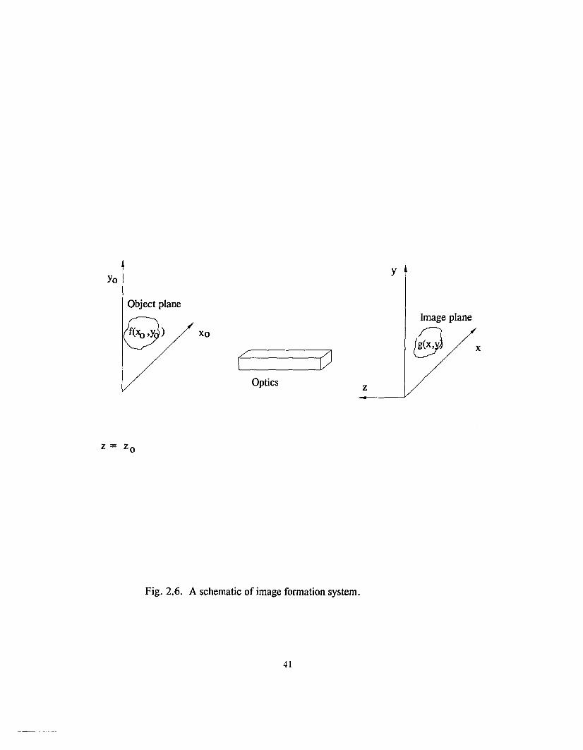
For a general representation of image formation (Fig. 2.6), consider the

general superposition integral for a blurred image formation (Andrews and Hunt

[1977]):

rt>rt>

g(x,y) = IIh(xo,yo,x,y,z(xo,yo),f(xo,yo» f'(xs.ys) dxs dyo (2.3)_00_00

where g(x,y) represents the image brightness function for the blurred image in image

plane coordinates (x,y), f(xo'yo) is the brightness of a point on the object, Zo is the

range of a point (xo,Yo) on the object surface and h(xo,Yo,x,y,zo(xo,yo),f(xo,yo» is

the nonlinear, space variant PSF. For an image blurred only due to camera motion

along the x-axis of the image plane, Eq. (2.3) reduces to :

rt>

g(x) = I f'(xs) h(xo,x,Zo(Xo» dx,.rt>

(2.4)

For a set of non-obscuring surfaces where the distortion is only due to the blur

induced by uniform velocity of the camera along the x-axis, the point spread function

in Eq. (2.4) takes the following form:

40

Yo

Object plane

Sl

z = Zo

Xo

Optics z

y

Image plane

~ x

Fig. 2.6. A schematic of image formation system.

41

h(xo, x,Zo(xo»1 x-x.

- rect[--]D D

(2.5)

where D is the disparity or blur length as indicated in Eq. (2.1) and is a function of z,

f is the focal length, L is the total displacement of the camera from its initial to final

position, rect[ .. ] = 1 for xo<x<xo+D and zero for xsx, and x~xo+D. Ifthe current

discussion is limited to scenes that can be approximated as isoplanatic (constant range)

or as consisting of isoplanatic patches, Eq. (2.4) can be reduced to:

00

g(x) = J f(xo) . h(x - x.) dx,-00

where ® indicates convolution.

= f ® h (2.6)

Three methods for determining the disparity have been tested for the case of

spatially invariant blurring to determine their accuracy, computational efficiency and

robustness in the face of noise. In all cases we only consider a single raster scan line

or epipolar line under the assumption that the raster scan direction and the direction of

camera motion are aligned. It is also assumed that no new objects enter the scene

during the blur generation.

2.3.1 Minimization Approach

Since Eq. (2.1) relates the disparity to the range and Eq. (2.5) relates the

disparity to the blur function h(xo,x,zJ, the determination of range is reduced to a

search for the blur function. One way of accomplishing this is to arbitrarily select a

42

value for D and to convolve h with the acute image f to produce a synthetic blur

image, gs(x,y). We have selected the sum over all pixels of the absolute difference of

gray levels between the calculated and actual blur images as the error measure of the

guessed point spread function. A value of D can be determined which minimizes this

error.

2.3.2 Fourier Transform Approach

From Eq. (2.6) it can be noted that in the special case of constant disparity i.e.

constant range, the blur image is the convolution of the acute image and the space

invariant point spread function. This equation is also valid if the range varies with

respect to y alone. In addition if the scene consists of a foreground for which the

disparity is invariant in x, viewed against a uniformly bright background then the

background and foreground have appearance of being co-planar.

Sawchuk [1972, 1974] has demonstrated that a deconvolution procedure can be

used to recover a sharp image from a blurred image when the PSF is known.

Conversely, Fox [1988] has shown for synthetic images that a deconvolution process

yields the PSF and therefore the disparity, when the scene is isoplanatic or can be

approximated by a set of isoplanatic patches. Taking the Fourier transform of the

equation (2.6) and solving for the PSF yields:

h(xo- x) = F I { F[g(x,y)] }F{f(xo,yo)]

(2.7)

where F[gOl and F[f()] are the Fourier transforms of the blurred and acute image

respectively and F-10 represents the inverse Fourier transform.

43

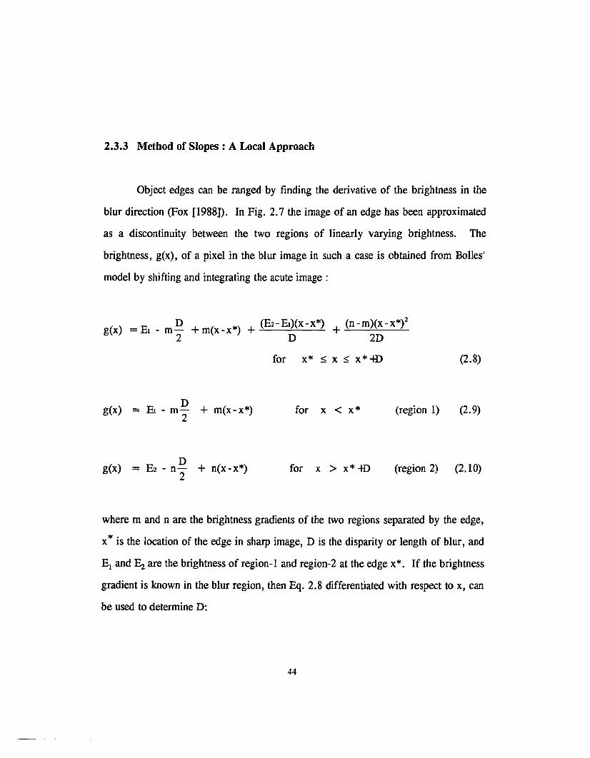
2.3.3 Method of Slopes: A Local Approach

Object edges can be ranged by finding the derivative of the brightness in the

blur direction (Fox [1988]). In Fig. 2.7 the image of an edge has been approximated

as a discontinuity between the two regions of linearly varying brightness. The

brightness, g(x), of a pixel in the blur image in such a case is obtained from Bolles'

model by shifting and integrating the acute image :

D (E2 - EI)(x -x*) (n - m)(x - X*)2g(x) = EI - m2" + m(x-x*) + D + 2D

g(x)D

= EI - m- + m(x-x*)2

for x* :s;; x :s;; x * -tD

for x < x* (region 1)

(2.8)

(2.9)

g(x)D

= E2 - n- + n(x-x*)2

for x > x*-ID (region 2) (2.10)

where m and n are the brightness gradients of the two regions separated by the edge,

x* is the location of the edge in sharp image, D is the disparity or length of blur, and

E1 and ~ are the brightness of region-I and region-2 at the edge x*. If the brightness

gradient is known in the blur region, then Eq. 2.8 differentiated with respect to x, can

be used to determine D:

44

'( ) + (E2-E.)+(n-m)(x-x*)g x =mD

for x* < x < x * -tD (2.11)

The next step is to test these decoding methods for robustness.

45

yRegion 1 Region 2

n

E2

Elm

x*

Fig. 2.7. An edge separating two regions of linearly varying brightness.

46

..

x

CHAPTER 3.

Tests for Robustness, Simulation and Real Image Analysis

3.1 Introduction

A preliminary study was carried out with simulated images to test the three

decoding methods for robustness. The simulated images included the simplest case

consisting of isoplanatic surfaces. The decoding methods found to be robust were

tested further using more complex surfaces. Since the blur is only in the x direction

i.e. the raster scan direction, a single raster line was generated and analyzed. The

rotating mirror system generating a blur image was also tested.

3.2 Tests for Simulated Rectangle Function Images

A rectangle function image was created (Fig. 3.1), simulating a raster scan

line of a uniformly bright planer object 30 pixels wide, on a gray background. The

background gray level was set to zero while the foreground object had a gray level

value of 10,000. The blur image was then created assuming that the planer surface

was parallel to the image plane (Fig. 3.2), by integrating a series of rightward shifted

images to produce a blur length of 10 pixels. The amplitude was then rescaled to

account for any shutter time difference between the blur and acute images.

The blur-acute pair were analyzed using the minimization algorithm, Fourier

transform method and slope method. Each yielded the correct disparity of 10 pixels

for the target described above.

12000

'"II) 8000.E'">

]>.e 4000e

Reet width = 30 pixels

Pixel Number

Fig. 3.1. Stationary image.

48

Rect width = 30 pixels

12000

1($=' 8000ca>Q)6)

...:l>. 4000~...o

oV'l-

O+-......,.............,.....~,...........--,..~...,....-..-Lr~--,--...,........L,...........--.--.-...,........--.-.....,....~o

Pixel Number

Fig. 3.2. Blurred image.

49

In order to better simulate the real images, noise was injected into the

synthetic images. Single pixel noise of gray level value of 10% of the magnitude of

the step function gray level, was added in the blurred image (Fig. 3.3) at pixel

number 200.

The minimization algorithm and the slope method still yielded the correct

disparity of 10 pixels. The point spread function obtained using the Fourier

deconvolution method is shown in Fig. 3.4. It can be seen that even a small amount

of noise has a pronounced effect on the calculated PSF. Although it is possible that

the correct disparity can be recovered with appropriate filtering of the result, at this

point it must be said that the method is not robust.

Gaussian noise with a mean value of 10% of the maximum image brightness

and a standard deviation of 5% was added to the blurred image. Both the

minimization and slope method still produced the correct disparity of 10 pixels. The

Fourier method yielded a result which was too noisy to interpret.

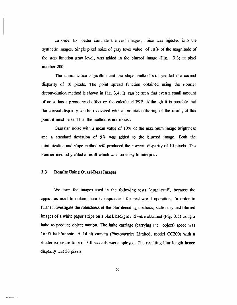
3.3 Results Using Quasi-Real Images

We term the images used in the following tests "quasi-real", because the

apparatus used to obtain them is impractical for real-world operation. In order to

further investigate the robustness of the blur decoding methods, stationary and blurred

images of a white paper stripe on a black background were obtained (Fig. 3.5) using a

lathe to produce object motion. The lathe carriage (carrying the object) speed was

16.05 inch/minute. A 14-bit camera (Photometries Limited, model CC200) with a

shutter exposure time of 3.0 seconds was employed. The resulting blur length hence

disparity was 33 pixels.

50

12000

~:s

8000'(U

>Q)

~~

~ 4000'"'e

00 0 8 0 8 0

\f") \f") In- - N N

Pixel Number

Fig. 3.3. Blurred image with a pixel noise (10% of the max.).

51

Pixel Number

Fig. 3.4. Point Spread Function (Fourier transform approach).

52

12000Stationary

..MImage

(...... ~ . --. Blurred Image

~ • •:l8000 •ca • ,

> , ,Q)

. •• ,6) • ,

...:l •~ 4000

, ,... , ,o . .

•./.- \

0

,0 0 8 0 8 0

lrl lrl lrl- - N N

Pixel Number

Fig. 3.5. Quasi-real images.

53

The minimization approach (Fig. 3.6) and slope method algorithms resulted in

the correct disparity of 33 pixels. As expected from noise tests the Fourier

deconvolution approach could not extract the disparity from the quasi-real images.

3.4 Blur Images From Rotating Mirror

A schematic of the experimental setup is shown in Fig. 3.7. An 8-bit CCD

camera (Pulnix America Inc., model TM-845) along with a frame grabber (Imaging

Technology Inc., Pcvision Plus) mounted in an IBM PCIAT was used for acquiring

the images. The rotating mirror system was fabricated by Lincoln Laser Company.

The mirror rotational speed was maintained at 30 rotations per second in synchronism

with video camera frame rate. A real blur image was acquired using a shutter speed of

114000 second and an optical axis displacement of 0.6623 inches. A paper target was

used consisting of a white stripe on a black background with range of 73.25 inches.

The resulting brightness profiles for a single raster scan line are shown in Fig. 3.8.

The stereo disparity determined by direct observation was 23 pixels.

Application of the minimization approach resulted in a disparity of 24 pixels,

while the method of slopes yielded 25 pixels. The Fourier deconvolution failed to

produce a discernible rectangle function.

3.5 Analysis

Analysis of simple images demonstrated that decoding of blur information to

obtain disparity can be accomplished with either an error minimization approach or by

analysis of the blur derivative. Fourier deconvolution appears not to be robust because

of its instability in presence of image noise. Both the error minimization methods and

54

oM

o-O+--~----,--~-----,------'---r--~--r--~

o

400000

';;;'Q) 300000~

....:l

~o 200000.S'-'....§ 100000~

BlurLength (in pixels)

Fig. 3.6. Results of minimization approach for quasi-real images.

Error = sum of the square of gray level values of

(Stationary-blurred - Blurred) image.

55

Line of Sight

Object Plane

Rotating Mirror-Square

/ IBM-pc

=

Camera

Fixed Corner Mirrors

Fig. 3.7. Schematic of the experimental setup.

56

80....... Blurred Image

f(S 60 Stationary:sImageCd

>Q) ~.,l,.. t',

40 . ~.,. '.&> .. . ..

,\....l .' ..>. " ..'" .''"" .. ..o 20 ,

~

," ..,

00 8 00 0 8 lI'l InlI'l - - N N

Pixel Number

Fig. 3.8. Real images.

57

the slope analysis have excellent noise tolerance. The method-of-slopes is better suited

for real time implementation due to its non-iterative nature. The rotating mirror

system designed to produce sawtooth shifting of the camera optical axis functioned as

predicted.

58

CHAPTER 4.

Experiments, Method of Slopes

4.1 Introduction

The preliminary tests described in chapter 3 demonstrated that the method-of­

slopes and the minimization approach are robust for decoding the disparity of.

isoplanatic surfaces. The non-iterative nature of the method-of-slopes indicates its

potential for real-time implementation. To fully explore the method-of-slopes, the

next logical step is to test it on an inclined plane and cylindrical surfaces.

4.2 Inclined Plane Surface

Consider a plane surface inclined at some angle 900-a to the camera optical

axis, as shown in Fig. 4.1. Pixel areas at a location Xi' Xi-l' xi_2' ... , xi-m' receive the

light intensity from surface patch areas dAj , dAi_l , dAj _2, ... , dAj_m+ l respectively.

The brightness intensity at a pixel Xi can be defined by:

I 1=1m dAif(xi) =- J Ei- cos(a) (I+tan(a)cot(¢;»

T 1=10 dx,(4.1)

where i is the pixel index, to and tm are the camera shutter opening and closing times,

T = lm-to is shutter time interval, & is the brightness of the surface patch area dAj

viewed by the pixel Xi of the area dx, a is the angle between the surface tangent and

the image plane, , is the angle between the ray joining the leading edge of a pixel to

Optical axis

z

motion ---

Object

a

Xjxi-l" x i-m+ 1 xImage plane

Fig. 4.1. Imaging of a plane surface inclined to the optical axis.

60

the corresponding surface patch and the image plane. A blur image is generated when

the plane travels across the camera during the camera shutter interval or vice versa. If

the inclined plane is assumed to have uniform relative motion from left to right (Fig.

4.1), then in the image plane, the total irradiance on a pixel Xi due to patches dAi ,

dAi_l, dAi_2 , ••• , dAi_m+ l, as they traverse across the ray from pixel Xi projected

through the lens center, is given by:

1 1 a II dAi 1 • b dAi _I

g(xJ=- [ JEi-. cos(a) (l+tan(a)cot(M) + JEi-I-.-cos(a) (l+tan(a)cot(¢t-I»T 1=10 dx, t=1I dx .:

1 =J"" dAi -m + I+ ... + E;.m+l. cos(a) (l+tan(a)cot(~-m+l» ]

1 = la.' dxr -m + I

(4.2)

where tl'~' ... , tm_1 are the intermediate time readings between to and tm • From Eq.

4.1, the brightness at any pixel Xi can be substituted for the brightness gray level in

the sharp image:

(4.3)

If the relative motion between camera and the surface patch is assumed to be

uniform then every point on the object will have a uniform velocity with respect to

the camera. This will result in uniform velocity of each image point in the image

plane. If Di, Di_l, Di_2, ••• , Di-m+1 are disparities and Vi' Vi_I' V i-2, ... , V i-m+1 are

velocities at sensor pixel Xi' Xi-I' Xi-2' ... , Xi-m+1 then the velocity is given by:

61

Vi = dx I. , Vi _I = dx I. I ' ... , Vi.m +1 = dx I.dt I dt 1- dt i-m-H

and shutter time can defined as:

(4.4)

or

DiT =

ViDi-IVi-I

Di-2=-- =

Vi-2

Di-m=--

Vi-m(4.5)

dx I1 =~T r»

= (4.6)

Substitution from Eq. 4.6 for shutter time into Eq. 4.3 results in:

( )_ Xf'lIf(Xi)d Xf'12f(Xi-l)d l+tan(a)cot(¢i-I)g Xi - -- X + X-----'-~---'-~-:..

x] D, x] Dr - I 1+ tan( a)cot(¢i)to II

~~ ~ )+ ... + f f(Xi-m+l) dx l+tan(a)cot('I"-m+lxl~., D:-m+J 1+tan(a)cot(tjI.)

Since cot(¢) = ~i (see Fig. 4.1), Eq. 4.7 can be written as:

XiII f xl12

g(xi) = f (Xi) dx + f f(Xi-l) dx 1+ Xi-] tan(a)

I D, I D, -J 1+ Xi tan( a)x to xli

xl~

+ ... + f f(Xi-m+l) dx 1+ Xi-m+J tan(a)

I Di-m+J 1+ xitan(a)X~.I

62

(4.7)

(4.8)

For angle of inclination <X approaching 90°, the inclined plane becomes a step edge.

Therefore, to take into account the imperfect step edges here we consider the surfaces

with a. s 80° as the inclined plane case. For a 14-bit CCD200 camera with focal

length f = 28 mm and pixel size of 0.02 mm, a blur length of 20 pixels from origin,

h f: 1+ Xi - m + I tan( a) 1 . h i 7 5% d .. h Eq 4 8 edt e actor == WIt 10 • 0 eviation. T e .. r uces to:1+ Xi tan(a)

g(x)= If(Xi) dx + 12f(Xi-t) dx + ... + l f(Xi-m+l) dx = l f(x) dx (4.9)

I Dt I Dr - t I D, -m + t vl._ DCX)X to X t l X Im•1 ~w

If the blur length of the last pixel across the ray from a pixel x and the camera lens

center is Dm then Eq. 4.9 takes the form:

g(X) = 1~(X) dxxi-Dm (x)

(4.10)

Note that the lower limit of integration involves Dm , which depends upon the range of

the pixel at location x-Dm• Equation 4.10 can be solved either by assuming that the

surface patch between pixel x and x-D; is isoplanatic (isoplanatic estimation

approach), or by estimating the blur at the starting point of a surface patch and

removing its contribution from successive pixels. In the second approach, the gray

level left at a pixel after the removal of previous blurs is the estimated blur gray level

at that pixel. Blur length is obtained by dividing the corresponding gray level value in

sharp image with the estimated blur gray level (intensity division approach). This

approach requires a starting point such as an edge discontinuity. The isoplanatic

estimation approach does not need a starting point. It should be noted here that in a63

blur image, the brightness intensity level is function of the angle of inclination a. and

the disparity. Physically, it is a problem of one equation with two unknowns, and we

need one constraint to solve it. At an edge between two inclined surfaces, the

brightness gray level in a blurred image is function of four unknowns: the angle of

inclination of the background and the foreground surfaces, and the disparity of the

background and the foreground surfaces. This case of one equation and four

unknowns can not be solved analytically.

Let us consider the edge problem in more detail. Figure 4.2 shows a blur­

acute pair containing a step edge between two uniformly varying brightness surfaces.

At the blurred edge, this pair does not indicate whether the right surface is moving

over the left surface, or the left surface is uncovering the right surface. The length of

the blurred edge region corresponds to the maximum of the two surface disparities. If

this maximum of two disparities is due to the surface under consideration, then the

remaining disparity values on the surface can be recovered. In a physical sense, at an

edge, the disparity of the background surface can not be recovered. To understand

this problem clearly, let us consider three consecutive surface patches overlapping

each other. At the edges, let us assume that the first surface is occluded by second,

and the second surface is occluded by the third. Let us also assume the algorithm

proceeds in a left to right direction. Since the length of the blurred edge region

between first and second surface is equal to the disparity of the second surface, and

the second surface is foreground as compared to the first surface, the disparity values

at the pixels on the second surface can be determined. Similarly, between the second

and the third surface, the length of the blurred edge region is equal to the disparity of

third surface, and the disparity values at the third surface (foreground surface) can be

determined. Now let us explore the other possible occlusion condition, in which the

64

GrayLevel

GrayLevel

Acute Image

surface 2

surface 1

Blurred Image

surface 2

surface 1

-/ I- blurred edge

Fig. 4.2. Blur-acute pair.

65

x

x

first surface occludes the ~ econd surface and the second surface occludes the third

surface. Since the length of the blurred region at the edge between first and second

surface is equal to the disparity of the first edge, and the second surface is

background as compared to the first surface, the disparity values at the pixels on the

second surface can not be determined. Similarly, at the edge between the second and

third surfaces, the third surface is background as compared to the first surface;

therefore, the disparity values at the pixels on the third surface can not be

determined. This problem dictates the need for the acute image at the other geometric

extreme (right hand acute image). Therefore, three images are needed to discern the

disparity at the edges and the corresponding surfaces: the left or beginning acute

image, the blurred image and right or end acute image.

4.3 Simulation and Analysis: Isoplanatic Approach

A blur-acute pair, containing three surface patches having brightness gradients

of 5, 20, 40 respectively, a y-axis intercept gray level value of 5000, and a uniform

disparity of 15 pixels, was created as shown in Fig. 4.3. Algorithm, using the

isoplanatic approach in the neighborhood of a pixel, resulted in the correct disparity

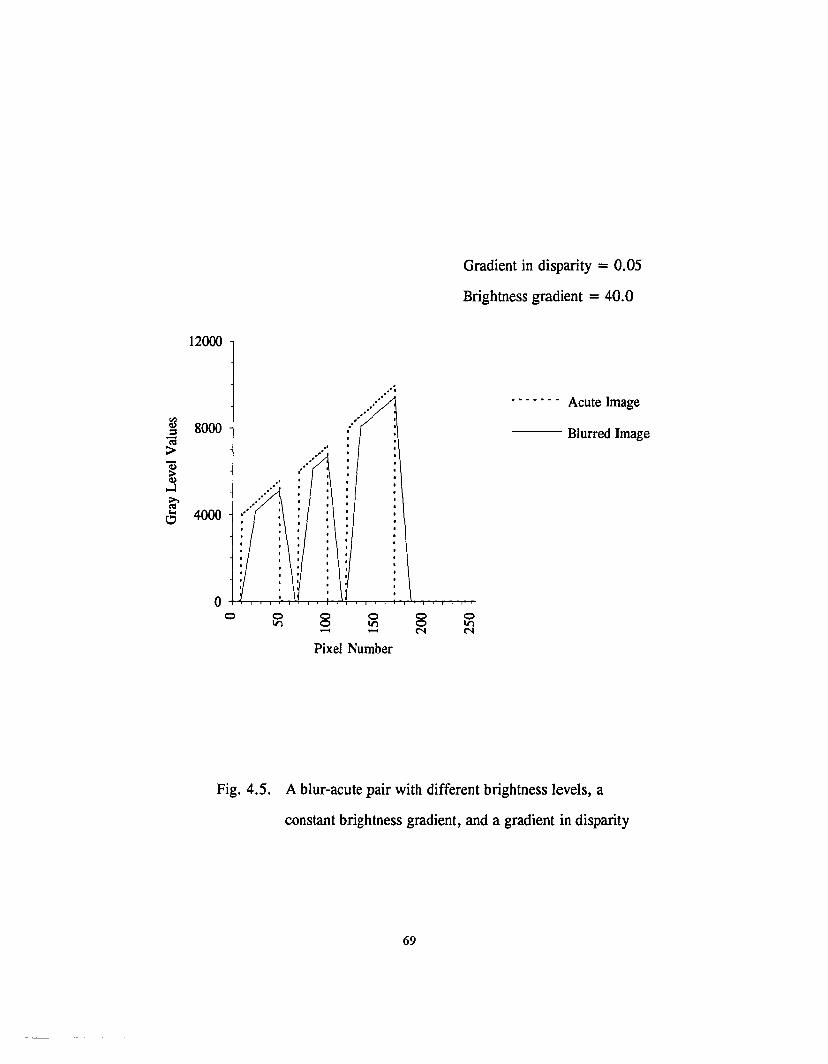
of 15 pixels (Fig 4.4). To increase the complexity a blur-acute pair containing three

surface patches, with different brightness gray levels but the same brightness

gradient of 40, and a gradient of 0.05 in disparity, was created (Fig. 4.5). The

isoplanatic approach resulted in disparity values exhibiting a staircase pattern as

expected (Fig. 4.6). The average gradient of the result approximates the actual

gradient but the absolute values have a shift.

A blur-acute pair containing three surface patches, with a gradient in

disparities of 0.2, 0.4 and 1.0 was created (Fig. 4.7). The actual and resultant

66

Variable Brightness Gradients of 5, 20 and 40

12000

&'S 8000=~

]g4000

o 8- ~-

. . . . . .• Acute Image

--- Blurred Image

Pixel Number

Fig. 4.3. A blur-acute pair with variable brightness gradient

67

20

Simulation

IsoplanaticApproach

~-8-

po--

5

oo

15

Pixel Number

Fig. 4.4. Disparity of isoplanatic surface patches with variable brightness gradient

68

Gradient in disparity = 0.05

Brightness gradient = 40.0

12000

Acute Image

--- Blurred Image

8N

~-

.',.......,......

8-O++--,---,---,-,-""\-r--r-+~..,-,-r-,.--+-~...,.-,....,....,-,-T"

o

8000

4000

Pixel Number

Fig. 4.5. A blur-acute pair with different brightness levels, a

constant brightness gradient, and a gradient in disparity

69

Gradient in disparity = 0.05

30

25

20>.

•t:: ~ ...... ..' ..........la0. 15til

(5

10

5

00 0 8 0 8 0

trl trl In- - N N

Pixel Number

Simulation

IsoplanaticApproach

Fig. 4.6. Results of blur-acute image pair with a gradient in disparity

70

12000

Acute Image

--- Blurred Image

olrlN

8N

olrl-

.'~....,..".

....".,

olrl

o ++-..,-r~~-,--,.---r-:~r-T---r--,-r--,-~.,-,-~~

o

~ 8000

~

Pixel Number

Fig. 4.7. A blur-acute pair for surfaces with different gradients in disparity

71

disparity values are shown in Fig. 4.8. The plot indicates that best fit gradient in

disparity approximates the actual disparity gradient, but the absolute disparity values

have an offset from the actual disparity values. Offset increases with the gradient.

Note that the oscillation in the disparity is due to the noise in the blurred image

resulting from truncation error.

Here one should note that the isoplanatic approximation concept does recover

the gradient in disparity, but the values are offset. The offset increases with the

increase in brightness level of the surface and the gradient in disparity.

4.4 Simulation and Analysis: Intensity Division Approach

To check the validity of this algorithm based on the intensity division

approach, preliminary tests were carried out on isoplanatic surfaces. A left acute

image, containing three overlapping surfaces of uniform gray levels 6000, 10000, and

8000 respectively, on a black background (Fig. 4.9), was generated. The three

surfaces were assigned a disparity of 10, 20, and 15 pixel lengths (Fig. 4.10), and

both a blurred and a right acute image were generated (Fig. 4.9). The inclined plane

algorithm, based on the intensity-division-approach produced the exact disparity

values of 10, 20, and 15 (Fig 4.11 and 4.12) associated with the three respective

surfaces. Figure 4.11 shows the results of the algorithm, on its traverse from left to

right, using the left acute and the blurred image. Figure 4.12 shows the results of the

algorithm on its traverse from right to left, using the right and the blurred image.

Tests with images containing three surfaces patches overlapping each other also

produced the actual disparity values. These results indicate that algorithm performs

well on isoplanatic surfaces.

72

Disparity gradients of 0.2, 0.4 and 1.0

140

120

100

.~ 80~

C':I

IE's 60

40

20

00

.......

8- o111-

.:..

Simulation

--- IsoplanaticApproach

Pixel Number

Fig. 4.8. Results for surfaces with three different disparity gradients

73

,,,

, ·,, ·, ·,· ·· · ·· · ·· · ·· · ·· · ,·, · ,· , ,. , , · ·, · , ,

, · , · ·· ·· · ,. , · · , I· · ·, · · ·, · , ·· ···

12000

~ 8000='ca>Q)

~,.J»~.... 40000

oo o

lrl 8- olrl- 8

N

--- Left AcuteImage

Blurred Image

Right AcuteImage

Pixel Number

Fig. 4.9. A blur-acute image set for a scene consisting of three isoplanatic

surfaces with different disparity and brightness levels

74

8

20

15

5

O+---'........~--,---J---r-.I,--r--r----r-+---,-~J,----,....-.-~---r---1-..,.-.,.--,r--r----r~o

Pixel Number

Fig. 4.10. Disparity for three isoplanatic surfaces.

75

20

15

--- Simulation

Intensity DivisionApproach

5

~-8-o ..J.--.+--r--1r-r--h--h-...,..-,--J-.r-r-J,-,-..,-,---ri-..--r-r--r--r--r­

o

Pixel Number

Fig. 4.11. Results of intensity division approach using

leftacute and blurred images

76

Simulation

- IntensityDivisionApproach

oIn-8-

, " ,

· ,, ,

·· ·· ,

· ,

·· ,"· · ," ,

· , · ,, , ,· , , ,· , ,· , , ·, , ,· , ·· , , ,

.- · · , · ,

· , · , ·· · , ,

· · · , · ·, , · , , ,

· · · , ·, ,

· · · · , ·, , · , ·· · , , ·, , · ·, · · , · ·· · · , , ·, · , · ·, · , , ·· · · , , ·, · , , ·· , · · ·oo

5

15

20

Pixel Number

Fig. 4.12. Results of intensity division approach using

right acute and blurred images

77

4.4.1 Inclined Plane

A blur-acute image set (Fig. 4.13) containing three overlapping surface

patches (Fig. 4.14) with respective brightness gradients of the order of 5, -7, and 8

was generated. The resultant disparity values, using the division of intensity

approach, is shown in Fig. 4.15. To more closely approximate real images, a

Gaussian noise of the order of 1% of the maximum gray level value was added in the

blur-acute image set (Fig. 4.16). The resultant plot of the recovered disparity values

is noisier (Fig. 4.17). The result from a blur-acute image set containing 5% Gaussian

noise is shown in Fig. 4.18. The plot depicts further degradation in disparity values.

Therefore, disparity degrades gradually with increase in noise.

4.4.2 Cylindrical Surface

A semi-cylindrical surface (included angle = 180°) occluding two inclined

plane surfaces (Fig. 4.19) at an angle of 45° and 135°, respectively, from a plane

perpendicular to camera optical axis, was generated. The blur-acute image set is

shown in Fig. 4.20. The intensity-division-approach produced a disparity values plot

as shown in Fig. 4.21. The result indicates a large deviation in values near the edge

of the semi-cylindrical surface, and the best fit disparity profile seems to follow the

actual disparity profile. Figure 4.22 and 4.23 show the results of a blur-acute image

set containing the semi-cylindrical surfaces, with included angle 175° and 170°

respectively. The results indicate that the deviation near the edge of the of the semi­

cylindrical surface has reduced. To more closely approximate the real images, a

Gaussian noise of the order of 1% of the maximum gray level (Fig. 4.24) was added

in the blur-acute image set. The results obtained by the algorithm (Fig. 4.25) show

78

Variable brightness gradients of 5, -7 and 8

12000

_.r.:::::-;~ ... ..

:: ,..-:.

~ ·,· ·,· ··· ·· ,

· ··· ·· ,

· ··

en8000<l)

='~v~>.~ 4000o

oo o

In 8- oIn- 8

N

--- Left AcuteImage

Blurred Image

--- Right Acute Image

Pixel Number

Fig. 4.13. A blur-acute image set for three inclined plane

surfaces with different brightness gradients

79

Range z is in em,

500

400 ------N 300

~~ 200 -----

100

00 50 100 150 200 250 300

Pixel Number

Fig. 4.14. Three inclined plane surfaces

80

35

Simulation

--- Left Traverse

--- Right Traverse

8N

otrl-8-

O+-O-"""""'I..Jl--,r-r-,.....,...,..L,-~'""""""-'""""+-.,...,."'l"""'-,.­

o

5

10

30

25

.~ 20!a~is 15

Pixel Number

Fig. 4.15. Results for three inclined plane surfaces

81

12000

~~.~\: .. ... ~..

..-.olI!'.

······, ,· ·,· ·· ,

, ,··

18 8000='~>Q)6)~

~.... 4000o

oo 8 o

It'l-

--- Left Acute Image

Blurred Image

Right AcuteImage

Pixel Number

Fig. 4.16. A blur-acute image set for three inclined plane surfaces with the

Gaussian noise of the order of 1% of the maximum gray level

82

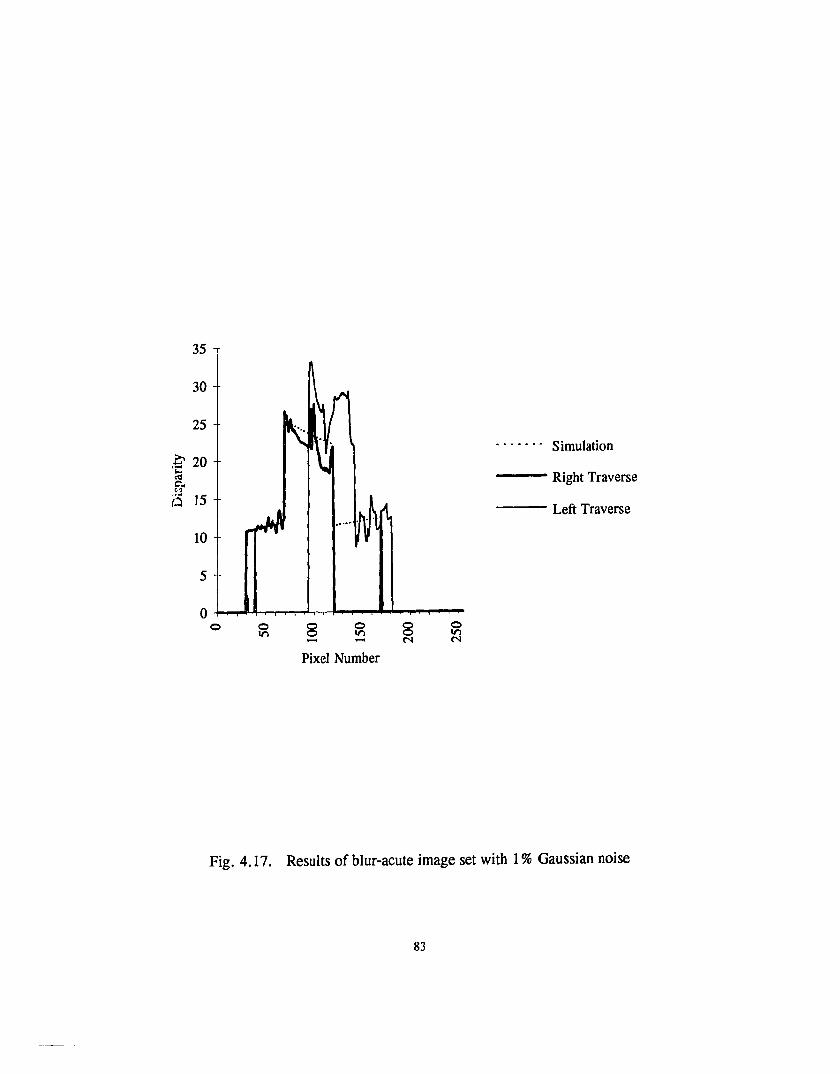
35

Right Traverse

Simulation

--- Left Traverse

8N

~-8-01o-o-..,....~'!"""'"""~.,-,-"""-~~~--­

o

5

10

30

25

.~ 20~

""<0is 15

Pixel Number

Fig. 4.17. Results of blur-acute image set with 1% Gaussian noise

83

35

Simulation

--- Left Traverse

--- Right Traverse

oIf'lN

8N

oIf'l-8-

O~""""'.If-.,....,....,...~.,..,.-+-.,.....,.....+-.,.....,.....,....

o

5

30

10

25

.~ 20;;c..<IJ

is 15

Pixel Number

Fig. 4.18. Results of blur-acute image set with 5% Gaussian noise

84

Included angle of the semi-cylindrical surface = 1800

Range z is in cm.

400

300

NQ)

~ 200~

100

300250200150

Pixel Number

10050

O+------,-------,-----.-------,-----r-----,

o

Fig. 4.19. Two inclined planes and a semi-cylindrical surface.

85

Included angle of the semi-cylindrical surface = 1800

10000

8000

~::sca6000>

2000 ····

--- Left Acute Image

Blurred Image

Right Acute Image

o\f"lN

8N

8O~'I"4-~-.-l-r--r-r...,.....,....--r.,..,-~~_.....

o

Pixel Number

Fig. 4.20. A blur-acute image set for two inclined planes

and a semi-cylindrical surface

86

35

30

25

.q 201:;;~Q 15

10

5

Simulation

--- Right Traverse

--- Left Traverse

8C'l

oIf'l-8-o

If'l

O~~--r-"..,-,.....,..L..--,--r-r-...,....,--.--I~~"'-'l""'!"''''''­

o

Pixel Number

Fig. 4.21. Results of inclined plane and semi-cylindrical surface

(included angle of the semi-cylindrical surface = 180°)

87

Simulation

--- Right Traverse

--- Left Traverse

8N

o.,.,-8-

5

01--"""""'"T"""T"-r-r--rl-r..,.,-..,.,-..,.,-~~~~.,-­

o

10

30

25

20

Pixel Number

Fig. 4.22. Results of inclined planes and a semi-cylindrical surface

(included angle of the semi-cylindrical surface = 175°)

88

Simulation

--- Left Traverse

--- Right Traverse

olI'l-8o

lI'l

5

o~---....,......-.--.--,-L,...,--r--r--r-r-.....--J.~~~---.­

o

10

30

35

25

.q 20!:a~a 15

Pixel Number

Fig. 4.23. Results of inclined planes and a semi-cylindrical surface

(included angle of the semi-cylindrical surface = 170°)

89

Included angle of the semi-cylindrical surface = 1700

ioooo

8000

~='C;; 6000>

Q)

~...:l>. 4000co:I....c:l

2000

--- Left Acute Image

Blurred Image

--- Right AcuteImage

otrlN

8N

otrl-8-

O~~...,....,,.,...,--.--.-.,............r-r-r.........~~"­o

Pixel Number

Fig. 4.24. A blur-acute image set for two inclined planes and a

semi-cylindrical surface with 1% Gaussian noise

90

Included angle of the semi-cylindrical surface = 1700

30

25

20

10

5

Simulation

--- Right Traverse

--- Left Traverse

oInN

8N

oIn-8o

In

0-1-o-~""""",,,,,,--,"""..,--r-y-r-r"""'''''''''''''''''_­

o

Pixel Number

Fig. 4.25. Results of inclined planes and a semi-cylindrical

surface in presence of 1% Gaussian noise

91

that the disparity values still follow the actual disparity profile. If the Gaussian noise

level is increased to 5% (Fig. 4.26) the result obtained is noisier (Fig. 4.27) but still

follows the actual disparity profile.

4.4.3 Quasi-Real Images

A quasi-real blur-acute image pair of a cylindrical object (Fig 4.28) was

obtained by mounting a 14-bit camera on a motor driven translational positioning

stage. The intensity- division-approach produced the results as shown in Fig. 4.29.

The best fit profile follows the actual disparity profile. Therefore, the intensity­

division-approach is robust in the face of noise.

92

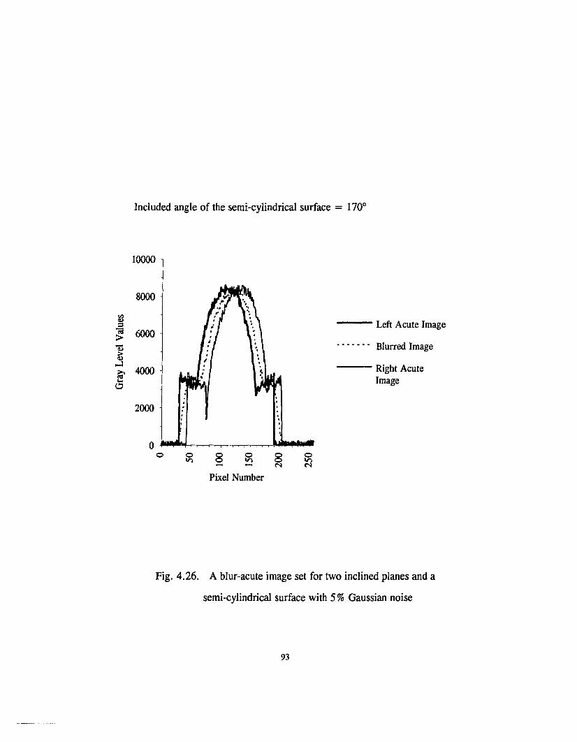
Included angle of the semi-cylindrical surface = 1700

ieoco

8000

r{S::sca 6000>

Q3

~...:l

~ 4000'""o

2000..

".0

0 0 8 0 8 0lrl lrl lrl- - N N

Pixel Number

--- Left Acute Image

Blurred Image

--- Right AcuteImage

Fig. 4.26. A blur-acute image set for two inclined planes and a

semi-cylindrical surface with 5% Gaussian noise

93

30

25

20Simulation

--- RightTraverse

--- Left Traverse

oII'l-

10 -

5

O~..,J.........-.....,...,.....,.J.""-'--~--r-T--.--l~~~----.,...,.

o

Pixel Number

Fig. 4.27. Results of inclined planes and a semi-cylindrical

surface in presence of 5% Gaussian noise

94

8000

60001($:::l

c.:l>'Q)

4000~.....l

~...o2000

····0

0 0 8 0 8 0Irl Irl II"l- - N N

Pixel Number

--- AcuteImage

Blurred Image

Fig. 4.28. A quasi-real blur-acute image pair of a cylindrical object

95

25

Actual

Intensity DivisionApproach

8N

olrl-8o

lrl

5

0+-t--.-,.~-,...eT-r--r-r-r-r--r-r...,.....,--4--,,.-,-,.-..-..-.-...-.­

o

20

o 15.~

~

t5 10

Pixel Number

Fig. 4.29. Results of quasi-real images of a cylindrical object

96

CHAPTER S.

Conclusion

5.1 Summary

The binocular disparity of a point in a scene is inversely proportional to the range.

This concept has been used to derive the range of an isoplanatic surface patch. A rotating.

mirror system was tested to generate blurred images. It produced the linearly blurred image

of an isoplanatic patch within ± 2 pixels for a blur length of 22 pixels. Three decoding

methods minimization approach, method of slopes and Fourier deconvolution approach, were

tested on simulated, quasi-real and real images. The method-of-slopes and the minimization­

approach were found to be robust. The non-iterative method-of-slopes was investigated

further for inclined plane surfaces. Algorithms based on brightness of a blurred image of an

inclined plane surface (Eq. 4.10) were developed and implemented using the isoplanatic

approach and the intensity-division approach. The isoplanatic approach was able to determine

the gradient of the disparity on the surface but the absolute values of the disparity were

offset. The offset increased with the increase in the gradient of the disparity and the level of

brightness. It was discovered that a right acute image is needed to decode a blur-acute image

set containing occluding surfaces. The intensity-division approach determined the disparity

values within ± 20% deviation. Addition of Gaussian noise produced noisier results. The

results degrade gradually with the increase in Gaussian noise level. Further tests on a semi­

cylindrical surface indicate that best fit profile approximates the actual disparity profile. The

results degrade gradually with the increase in Gaussian noise level. A test with a real image

of a cylindrical surface produced disparity values closer to the actual values.

The blur-acute image set can be acquired in one frame time, and the main problem

remaining is to recover disparity. Advent of faster and smaller computers will reduce the

computation time drastically. Therefore, the intensity division approach has potential for real

time implementation

5.2 Assumptions and Limitations

(1) Time it takes the camera shutter to open and close is very small as compared to the total

shutter time.

(2) Relative motion of the camera is uniform and parallel to the image plane.

(3) Objects in a scene consist of smooth and lambertion surfaces.

(4) Inclined plane surface equation assumes that the surface distortion effect is negligible.

(5) Method-of-slopes assumes that angle of inclination of an inclined plane should be less

than or equal to 80°.

5.3 Future Work

(1) As a first step toward real time implementation the rotating mirror system should be

integrated with the 14-bit camera controller to synchronize the camera shutter timings with

the rotational speed of the mirror cube.

(2) Since the method-of-slopes algorithm using isoplanatic approach works nicely on the

interior of a surface patch to provide the gradient of the inclined plane surface and the stereo

method provides the results at the edges, a combination of the two could be tested.

(3) Method-of-slopes using intensity-division approach should be tested further on more

complex images containing surfaces of arbitrary curvature.

98

REFERENCES

Andrews, H.C. and B.R Hunt, Digital Image Restoration. Prentice Hall, New York,

NY (1977).

Altschuler, M.D., B.R Altschuler and J. Taboada, "Laser electro-optic system for

rapid three-dimensional (3-D) topographic mapping of surfaces." Optical

Engineering, 20(6), 953-961, (1981).

Baker, H.H. and RC. Bolles, "Generalizing epipolar-plane image analysis on the

spatiotemporal surface." Proceedings of The Computer Society Conference on

Computer Vision and Pattern Recognition, Ann Arbor, Michigan, 2-9, (1988).

Ballard, D.H. and C.M. Brown, Computer Vision. Prentice Hall, Inc., New Jersey,

(1982).

Barnard, S.T. and W.B. Thompson, "Disparity analysis of images." IEEE

Transactions on Pattern Analysis and Machine Intelligence, PAMI-2(4), 333-340,

(1980).

Beheim, G., and K. Fritsch, "Range finding using frequency-modulated laser diode."

Applied Optics, 25(9), 1439-1442, (1986).

Begin, G., "Real time large depth of field 3-D vision system." SPIE, Imaging

Applications in the Work World, 900, 25-31, (1988).

Besl, P.J., "Active, optical range imaging sensors." Machine Vision andApplications,

1, 127-152, (1988).

Bicknel G., G. Hausler and M. Maul, "Triangulation with expanded range of depth."

Optical Engineering, 24(6), 975-977, (1985).

Bolles, R.C., H.H. Baker and D.H. Marimont, "Epipolar-plane image analysis: An

approach to determining structure from motion." International Journal of Computer

Vision, 1, 7-55, (1988).

Boyer, K.L. and A.C. Kak, "Color-encoded structured light for rapid active

ranging." IEEE Transactions on Pattern Analysis and Machine Intelligence, PAMI­

9(1), 14-28, (1987).

Chavel, P. and T.C. Strand, "Range measurement using Talbot diffraction imaging of

gratings." Applied Optics, 23(6), 862-871, (1984).

Church, E.L., T.V. Vorburger and J.C. Wyant, "Direct comparison of mechanical

and optical measurements of the finish of precision machined optical surfaces."

Optical Engineering, 24(3), 388-395, (1985).

Cline, H.E., A.S. Holik and W.E. Lorenson, "Computer-aided reconstruction of

interference contours." Applied Optics, 21(24),4481-4489, (1982).

Cline, H.E., W.E. Lorenson and A.S. Holik, "Automated moire contouring."

Applied Optics, 23(10), 1454-1459, (1984).

100

Dandliker R. and R. Thalman, "Heterodyne and quasi-heterodyne holographic

interferometry." Optical Engineering, 24(5), 824-831, (1985).

Dantu, R.V., N.J. Dimopoulos, R.V. Patel and A.J. Al-Khalili, "Depth perception

using blurring and its application in VLSI wafer probing." ASME Press Series:

Robotics and Manufacturing-3, 260-168, (1990).

Faugeras, D.D., and M. Hebert, "The representation, recognition, and locating of 3­

D objects. " International Journal ofRobotics Research, 5(3), 27-52, (1986).

Fairhurst, M.G., Computer Vision for Robotic Systems. An Introduction, Prentice

Hall International Ltd., (1988).

Fox, I.S., "Range from translational motion blurring." Proceedings of The Computer

Society Conference on Computer Vision and Pattern Recognition, Ann Arbor,

Michigan, (1988).

Gasvik, K.J., "Moire technique by means of digital image processing." Applied

Optics, 22(23), 3543-3548, (1983).

Gibson, J.l., The perception of the visual world. Houghton Mifflin Company, The

Riverside Press, Cambridge, Massachusetts, (1950).

101

Grimson, W.E.L., "Computational experiments with a feature based stereo

algorithm." IEEE Transactions on Pattern Analysis and Machine Intelligence, PAMI­

7(1), 17-34, (1985).

Grossman, P., "Depth from focus." Pattern Recognition Letters, 5, 63-69, (1987).

Hariharan, P., "Quasi-heterodyne hologram interferometry." Optical Engineering,

24(4), 632-638, (1985).

Hausler, G. and M. Maul, "Telecentric scanner for 3-D sensing." Optical

Engineering, 24(6), 978-980, (1985).

Hom, RK.P., Robotvision. The MIT Press, McGraw-Hill Book Company, (1986).

Hom, RK.P. and K. Ikeuchi, "Numerical shape from shading and occluding

boundaries." Artificial Intelligence, An International Journal, 17(1-3), 141-184,

(1981).

Hom, RK.P. and RG. Schunk, "Determining Optical Flow." Artificial lmelligence,

An International Journal, 17(1-3), 185-203, (1981).

Ikeuchi, K., "Determining a depth map using a dual photometric stereo." The

International Journal ofRobotics Research, 6(1),15-31, (1987).

102

Ikeuchi, K. and B.K.P. Horn, "An application of the photometric stereo method."

Proceedings 6th International Joint Conference on Artificial Intelligence, 413-415,

(1979).

Jaliko, J.A., R.C. Kim and S.K. Case "Three dimensional inspection using

multistripe structured light." Optical Engineering, 24(6), 966-974, (1985).

Jarvis, R.A., "A perspective on range finding techniques for computer vision." IEEE

Transactions on Pattern Analysis and Machine Intelligence, PAMI-5(2), 122-139,

(1983).

Jarvis, R.A., "A laser time-of-flight range scanner for robotic vision." IEEE

Transactions on Pattern Analysis and Machine Intelligence, PAMI-5(5), 505-512,

(1983a).

Jenkins, F.A. and H.E. White, Foundations of physical optics. McGraw-Hill Book

Company, 59-65, (1937).

Julesz, B., Foundations of Cyclopean Perception. The University of Chicago Press,

Chicago and London, (1971).

Kanade, T. and H. Asada, "Non contact visual three-dimensional ranging devices."

SPIE; 3-D Machine Perception, 283, 48-53, (1981).

103

Kender, J.R., "Shape from texture: An aggregation transform that maps a class of

texture into surface orientation." Proceedings 6th International Joint Conference on

Artificial Intelligence, 1, 475-480, (1979).

Krotkov, E., and J.P. Martin, "Range from focus." Proceedings IEEE International

Conference on Robotics andAutomation IEEE-CS, New York, 1093-1098, (1986).

Leger, J.R. and M.A. Snyder, "Real-time depth measurement and display using

Fresnel diffraction and white-light processing." Applied Optics, 23(10), 1655-1669,

(1984).

Leith, E. and J. Upatneiks, "Reconstructed wave fronts and communication theory."

Journal ofOptical Society ofAmerica, 54, 1123-1130, (1962).

Leung, M.K. and T.S. Huang, "Detecting wheels of vehicle in stereo images." IEEE

10th International Conference on Pattern Recognition, 1, 263-267, (1990).

Lewis, RA. and A.R Johnston, "A scanning laser range finder for a robotic

vehicle." Proceedings 5th International Joint Conference on Artificial Intelligence,

762-768, (1977).

Matthies, L., R Szeliski and T. Kanade, "Incremental estimation of dense depth

maps from image sequences." Proceedings of The Computer Society Conference on

Computer Vision and Pattern Recognition, Ann Arbor, Michigan, 366-374, (1988).

104

Moravec, H.P., "Visual mapping by a robot rover." Proceedings 6th International

Joint Conference on Artificial Intelligence, 598-600, (1979).

Moravec, H.P., "Rover visual obstacle avoidance." Proceedings 7th International

Joint Conference on Artificial Ituelligence, 785-790, (1981).

Nevita, R. and T.O. Binford, "Structured descriptions of complex objects."

Proceedings 3rd International Joint Conference on Artificial Intelligence, 641-647,

(1973).

Nitzan, D., A.E. Brian and R.O. Duda, "The measurement and use of registered

reflectance and range data in scene analysis." Proceedings IEEE, 65(2), 206-220,

(1977).

Ohta, Y.!., K. Maenobu and T. Sakai, "Obtaining surface orientations from texels

under perspective projection." Proceedings 7th International Joint Conference on

Artificial lntelligence, 746-751, (1981).

Ozeki, 0., T. Nakano and S. Yamamoto, "Real-time range measurement device for

three-dimensional object recognition." IEEE Transactions on Pattern Analysis and

Machine Intelligence, PAMI-8(4), 550-554, (1986).

Pentland, A.P., "A new sense for depth of field." Proceedings of International Joint

Conference on Artificial Intelligence, Los Angeles, CA, 2, 988-994, (1985).

105

Pentland, A.P., "A new sense for depth of field." IEEE Transaction on Pattern

Analysis and Machine Intelligence, PAMI 9(4), 523-531, (1987).

Pipitone, F.I. and T.G. Marshall, "A wide-field scanning triangulation range finder

for machine vision." The International Journal of Robotics Research, 2(1), 39-49,

(1983).

Popplestone, R.I., C.M. Brown, A.P. Ambler and G.F. Crawford, "Forming models

of plane-and-cylinder faceted bodies from light stripes." Proceedings 4th International

Joint Conference onArtificial Intelligence, 664-668, (1975).

Potmesil, M., "Generating models of solid objects by matching 3D surface

segments." Proceedings 8th International Joint Conference on Artificial Intelligence,

1089-1093, (1983).

Prazdny, K., "Motion and structure from optical flow." Proceedings of the

International Joint Conference on Artificial Intelligence, 702-704, (1979).

Pryputniewicz, R.I., "Heterodyne holography applications in studies of small

components. II Optical Engineering, 24(5), 849-855, (1985).

Roach, I.W., and I.K. Aggarwal, "Computer tracking of objects moving in space."

IEEE Transaction on Pattern Analysis and Machine Intelligence, PAMI-l(2) , 127­

135, (1979).

106

Roach, J.W., and J.K. Aggarwal, "Determining the movement of objects from a

sequence of images." IEEE Transaction on Pattern Analysis and Machine

Intelligence, PAMI 2(6), 554-562, (1980).

Sanz, J.L.C., Advances in Machine Vision. Springer-Verlag New York Inc., (1989).

Sato, Y., H. Kitagawa and H. Fujita, "Shape measurement of curved objects using

multiple slit-ray projections." IEEE Transaction on Pattern Analysis and Machine

Intelligence, PAMI 4(6), 641-646, (1982).

Sawchuk, A.A., "Space-variant image motion degradation and restoration."

Proceedings. IEEE, 60, 854-861, (1972).

Sawchuk, A.A., "Space-variant image restoration by coordinate transformations."

Journal ofthe Optical Society ofAmerica. 64(2), 138-144, (1974).

Shirai, Y., "Recognition of polyhedron with a range finder." Pattern Recognition, 4,

243-250, (1972).

Strand, T.C., "Optics for machine vision." SPIE, Optical Computing, 456, 86-93,

(1984).

Strand, T.C., "Optical three-dimensional sensing for machine vision." Optical

Engineering, 24(1), 33-40, (1985).

107

Subbarao, M., "Direct depth recovery of depth-map I: Differential methods."

Proceedings of IEEE Computer Society Workshop on Computer Vision, Miami Beach,

58- 65, (1987).

Subbarao, M., and N. Gurumoorthy, "Depth recovery from blurred edges."

Proceedings of The Computer Society Conference on Computer Vision and Pattern

Recognition, Ann Arbor, Michigan, 498-503, (1988).

Svetkoff, D.J., "Towards a high resolution, video rate, 3D sensor for machine

vision." SPIE, Optics, Illumination, and Image Sensing for Machine Vision, 728,

216-226, (1986).

Thalman, R. and R. Dandliker, "Holographic contouring using electronic phase

measurement." Optical Engineering, 24(6), 930-935, (1985).

Thorpe, C.E., Vision and Navigation, The Carnegie Mellon Navlab. Kluwer

Academic Publishers, Massachusetts, (1990).

Tozer, B.A., R. Glanville, A.L. Gordon, M.J. Little, J.M. Webster and D.G.

Wright, "Holography applied to inspection and measurement in an industrial

environment." Optical Engineering, 24(5), 746-753, (1985).

Trevor, D., and K. Wohn, "Pyramid based depth from focus." Proceedings of The

Computer Society Conference on Computer Vision and Pattern Recognition, Ann

Arbor, Michigan, 504-509, (1988).

108

Wagner, J.F., "Sensors for dimensional measurement." Proceedings of Vision '87

Conference, Michigan, 13(1), 13-18, (1987).

Webb, I.A. and J.K. Aggarwal, "Structure and motion of rigid and jointed objects."

Artificial Intelligence, 19(1), 107-130, (1982).

Weissman, M.A., "3-D measurements from video stereo pairs." SPIE, Three­

Dimensional Imaging andRemote Sensing Imaging, 902, 85-86, (1988).

Williams, T.D., "Depth from camera motion in a real world scene." IEEE

Transaction on Pattern Analysis and Machine Intelligence, PAMI 2(6), 511-516,

(1980).

Winthrop, J.T. and C.R. Worthington, "Theory of plane image I. Plane periodic

objects in monochromatic light." Journal of Optical Society ofAmerica, 55(4), 373­

381, (1965).

Witkin, A.P., "Recovering surface shape and orientation from texture." Artificial

Intelligence, 17, 17-45, (1981).

Wuerker, R.F., and D.A. Hill, "Holographic microscopy." Optical Engineering,

24(3), 480-484, (1985).

109