HAL Id: hal-01277624https://hal.inria.fr/hal-01277624

Submitted on 22 Feb 2016

HAL is a multi-disciplinary open accessarchive for the deposit and dissemination of sci-entific research documents, whether they are pub-lished or not. The documents may come fromteaching and research institutions in France orabroad, or from public or private research centers.

L’archive ouverte pluridisciplinaire HAL, estdestinée au dépôt et à la diffusion de documentsscientifiques de niveau recherche, publiés ou non,émanant des établissements d’enseignement et derecherche français ou étrangers, des laboratoirespublics ou privés.

Fast Robust PCA on GraphsNauman Shahid, Nathanael Perraudin, Vassilis Kalofolias, Gilles Puy, Pierre

Vandergheynst

To cite this version:Nauman Shahid, Nathanael Perraudin, Vassilis Kalofolias, Gilles Puy, Pierre Vandergheynst. FastRobust PCA on Graphs. IEEE Journal of Selected Topics in Signal Processing, IEEE, 2016, 10 (4),pp.740 - 756. 10.1109/JSTSP.2016.2555239. hal-01277624

Fast Robust PCA on Graphs

Nauman Shahid∗, Nathanael Perraudin, Vassilis Kalofolias, Gilles Puy†, Pierre VandergheynstEmail: nauman.shahid, nathanael.perraudin, vassilis.kalofolias, pierre.vandergheynst@epfl.ch, † gilles.puy@inria.fr

Signal Processing Laboratory 2 (LTS2), EPFL STI IEL, Lausanne, CH-1015, Switzerland.† INRIA Rennes - Bretagne Atlantique, Campus de Beaulieu, FR-35042 Rennes Cedex, France

Data X with corruptions

pfe

ature

s

n samples

G1 : Graph of data similarity

G2 : Graph of feature similarity

Lap

laci

anL 1

Lapla

cian

L 2

min U

kX

Uk 1

+1tr

(UL 1

UT)+

2tr

(UTL 2

U)

Low Rank U

Sparse X U

class 1

Class 2

Principal Component 1

Prin

cipa

l Com

pone

nt 2

Main idea of Fast Robust PCA on Graphs

Clu

ster

ing

onW

SV

D:U

=V

W>

Abstract—Mining useful clusters from high dimensional datahas received significant attention of the computer vision andpattern recognition community in the recent years. Linear andnon-linear dimensionality reduction has played an importantrole to overcome the curse of dimensionality. However, oftensuch methods are accompanied with three different problems:high computational complexity (usually associated with the nu-clear norm minimization), non-convexity (for matrix factorizationmethods) and susceptibility to gross corruptions in the data. Inthis paper we propose a principal component analysis (PCA)based solution that overcomes these three issues and approximatesa low-rank recovery method for high dimensional datasets. Wetarget the low-rank recovery by enforcing two types of graphsmoothness assumptions, one on the data samples and the otheron the features by designing a convex optimization problem. Theresulting algorithm is fast, efficient and scalable for huge datasetswith O(n log(n)) computational complexity in the number of datasamples. It is also robust to gross corruptions in the datasetas well as to the model parameters. Clustering experimentson 7 benchmark datasets with different types of corruptionsand background separation experiments on 3 video datasetsshow that our proposed model outperforms 10 state-of-the-artdimensionality reduction models. Our theoretical analysis provesthat the proposed model is able to recover approximate low-rankrepresentations with a bounded error for clusterable data.

Keywords—robust PCA, graph, structured low-rank representa-tion, spectral graph theory, graph regularized PCA

I. INTRODUCTION

In the modern era of data explosion, many problemsin signal and image processing, machine learning and pat-tern recognition require dealing with very high dimensional

datasets, such as images, videos and web content. The datamining community often strives to reveal natural associationsor hidden structures in the data. Over the past couple ofdecades matrix factorization has been adopted as one of thekey methods in this context. Given a data matrix X ∈ Rp×nwith n p-dimensional data vectors, the matrix factorization canbe stated as determining V ∈ Rp×c and W ∈ Rc×n such thatX ≈ VW under different constraints on V and W .

How can matrix factorization extract structures in the data?The answer to this question lies in the intrinsic associationof linear dimensionality reduction with matrix factorization.Consider a set of gray-scale images of the same object capturedunder fixed lighting conditions with a moving camera, or a setof hand-written digits with different rotations. Given that theimage has m2 pixels, each such data sample is represented bya vector in Rm2

. However, the intrinsic dimensionality of thespace of all images of the same object captured with smallperturbations is much lower than m2. Thus, dimensionalityreduction comes into play. Depending on the application andthe type of data, one can either use a single linear subspace toapproximate the data of different classes using the standardPrincipal Component Analysis (PCA) [1], a union of lowdimensional subspaces where each class belongs to a differentsubspace (LRR and SSC) [10], [21], [39], [34], or a positivesubspace to extract a positive low-rank representation of thedata (NMF) [20]. The clustering or community detection canthen be performed on the retrieved data representation inthe low dimensional space. Not surprisingly, all the abovementioned problems can be stated in the standard matrixfactorization manner as shown in the models 1 to 3 of Fig. 1.Alternatively, the clustering quality for non-linearly separable

datasets can be improved by using non-linear dimensionalityreduction tools such as Laplacian Eigenmaps [4] or KernelPCA [33].

In many cases low dimensional data follows some addi-tional structure. Knowledge of such structure is beneficial, aswe can use it to enhance the representativity of our models byadding structured priors [14], [23], [40]. A nowadays standardway to represent pairwise affinity between objects is by usinggraphs. The introduction of graph-based priors to enhance ma-trix factorization models has recently brought them back to thehighest attention of the data mining community. Representationof a signal on a graph is well motivated by the emerging fieldof signal processing on graphs, based on notions of spectralgraph theory [37]. The underlying assumption is that high-dimensional data samples lie on or close to a smooth low-dimensional manifold. Interestingly, the underlying manifoldcan be represented by its discrete proxy, i.e. a graph. LetG = (V, E) be a graph between the samples of X , where Eis the set of edges and V is the set of vertices (data samples).Let A be the symmetric matrix that encodes the weightedadjacency information between the samples of X and D isthe diagonal degree matrix with Dii =

∑j Aij . Then the

normalized graph Laplacian L that characterizes the graph G isdefined as L = D−1/2(D−A)D−1/2. Exploiting the manifoldinformation in the form of a graph can be seen as a method ofincorporating local proximity information of the data samplesinto the dimensionality reduction framework, that can enhancethe clustering quality in the low-dimensional space.

A. Focus of this work

In this paper, we focus on the application of PCA toclustering, projecting the data on a single linear subspace. Wefirst describe PCA and its related models and then elaborateon how the data manifold information in the form of a graphcan be used to enhance standard PCA. Finally, we present anovel, convex, fast and scalable method for PCA that recoversthe low-rank representation via two graph structures. Ourtheoretical analysis proves that the proposed model is able torecover approximate low-rank representations with a boundederror for clusterable data, where the number of clusters is equalto the rank. Many real world datasets can be assumed to satisfythis assumption. For example, the USPS dataset which consistsof ten digits. We call such data matrices as low-rank matriceson graphs. The clustering on these dataset can be done byrecovering a clean low-rank representation.

B. PCA and Related Work

For a dataset X ∈ Rp×n with n p-dimensional data vectors,standard PCA learns the projections or principal componentsW ∈ Rc×n of X on a c-dimensional orthonormal basis V ∈Rp×c, where c < p by solving model 3 in Fig. 1. Thoughnon-convex, this problem has a global minimum that can becomputed using Singular Value Decomposition (SVD), givinga unique low-rank representation U = VW .

A main drawback of PCA is its sensitivity to heavy-tailednoise due to the Frobenius norm in the objective function.Thus, a few strong corruptions can result in erratic principalcomponents. Robust PCA (RPCA) proposed by Candes et al.[7] overcomes this problem by recovering the clean low-rank

representation U from grossly corrupted X by solving model4 in Fig. 1. Here S represents the sparse matrix containing theerrors and ‖U‖∗ denotes the nuclear norm of U , the tightestconvex relaxation of rank(U).

Recently, many works related to low-rank or sparse repre-sentation recovery have been proposed to incorporate the datamanifold information in the form of a discrete graph into thedimensionality reduction framework [16], [44], [11], [6], [38],[18], [17], [28], [9]. In fact, for PCA, this can be consideredas a method of exploiting the local smoothness information inorder to improve clustering quality. The graph smoothness ofthe principal components W using the graph Laplacian L hasbeen exploited in various works that explicitly learn W andthe basis V . We refer to such models as factorized models.In this context Graph Laplacian PCA (GLPCA) was proposedin [16] (model 5 in Fig. 1) and Manifold Regularized MatrixFactorization (MMF) in [44] (model 6 in Fig. 1). Note that theorthonormality constraint in this model is on V , instead of theprincipal components W . Later on, the authors of [34] havegeneralized robust PCA by incorporating the graph smoothness(model 7 in Fig. 1) term directly on the low-rank matrix insteadof principal components. They call it Robust PCA on Graphs(RPCAG).

Models 4 to 8 can be used for clustering in the lowdimensional space. However, each of them comes with its ownweaknesses. GLPCA [16] and MMF [44] improve upon theclassical PCA by incorporating graph smoothness but they arenon-convex and susceptible to data corruptions. Moreover, therank c of the subspace has to be specified upfront. RPCAG[34] is convex and builds on the robustness property of RPCA[7] by incorporating the graph smoothness directly on thelow-rank matrix and improves both the clustering and low-rank recovery properties of PCA. However, it uses the nuclearnorm relaxation that involves an expensive SVD step in everyiteration of the algorithm. Although fast methods for the SVDhave been proposed, based on randomization [41], [22], [26],Frobenius norm based representations [43], [27] or structuredRPCA [2], its use in each iteration makes it hard to scale tolarge datasets.

C. Our Contributions

In this paper we propose a fast, scalable, robust and con-vex clustering and low-rank recovery method for potentiallycorrupted low-rank signals. Our contributions are:

1) We propose an approximate low-rank recoverymethod for corrupted data by utilizing only the graphsmoothness assumptions both between the samplesand between the features.

2) Our theoretical analysis proves that the proposedmodel is able to recover approximate low-rank repre-sentations with a bounded error for clusterable data,where the number of clusters is equal to the rank.We call such a data matrix a low-rank matrix on thegraph.

3) Our model is convex and although non-smooth it canbe solved efficiently, that is in linear time in thenumber of samples, with a few iterations of the well-known FISTA algorithm. The construction of the twographs costs O(n log n) time, where n is the numberof data samples.

M

GManifold information in Graph Laplacian LPCA

X 2 Rp

Graph Regularized PCA

Standard Matrix Factorization

Fig. 1. A summary of the matrix factorization methods with and without graph regularization. X ∈ Rp×n is the matrix of n p-dimensional data vectors,V ∈ Rp×c and W ∈ Rc×n are the learned factors. U ∈ Rp×n is the low-rank matrix and S ∈ Rp×n is the sparse matrix. ‖ · ‖F , ‖ · ‖∗ and ‖ · ‖1 denotethe Frobenius, nuclear and `1 matrix norms respectively. The data manifoldM information can be leveraged in the form of a discrete graph G using the graphLaplacian L ∈ Rn×n resulting in various Graph Regularized PCA models.

4) The resulting algorithm is highly parallelizable andscalable for large datasets since it requires only themultiplication of two sparse matrices with full vectorsand elementwise soft-thresholding operations.

5) Our extensive experimentation shows that the recov-ered close-to-low-rank matrix is a good approxima-tion of the low-rank matrix obtained by solving theexpensive state-of-the-art method [34] which uses themuch more expensive nuclear norm. This is observedeven in the presence of gross corruptions in the data.

D. Connections and differences with the state-of-the-art

The idea of using two graph regularization terms haspreviously appeared in the work of matrix completion [19],co-clustering [12], NMF [35], [5] and more recently in thecontext of low-rank representation [42]. However, to the best ofour knowledge all these models aim to improve the clusteringquality of the data in the low-dimensional space. The co-clustering & NMF based models which use such a scheme[12], [35] suffer from non-convexity and the works of [19] and[42] use a nuclear-norm formulation which is computationallyexpensive and not scalable for big datasets. Our proposedmethod is different from these models in the following sense:

• We do not target an improvement in the low-rankrepresentation via graphs. Our method aims to solelyrecover an approximate low-rank matrix with dual-graph regularization only. The underlying motivationis that one can obtain a good enough low-rank rep-resentation without using expensive nuclear norm ornon-convex matrix factorization. Note that the NMF-based method [35] targets the smoothness of factorsof the low-rank while the co-clustering [12] focuseson the smoothness of the labels. Our method, on theother hand, targets directly the recovery of the low-rank matrix, and not the one of the factors or labels.

• We introduce the concept of low-rank matrices ongraphs and provide a theoretical justification for thesuccess of our model. The use of PCA as a scalable

and efficient clustering method using dual graph reg-ularization has surfaced for the very first time in thispaper.

A summary of the notations used in this paper is presentedin Tab. I. We first introduce our proposed formulation and itsoptimization solution in Sections II & II-A and then developa sound motivation of the model in Section IV.

TABLE I. A SUMMARY OF NOTATIONS USED IN THIS WORK

Notation Terminology‖ · ‖F matrix frobenius norm‖ · ‖1 matrix `1 normn number of data samplesp number of features / pixelsc dimension of the subspacek number of classes in the data set

X ∈ Rp×n data matrixU ∈ Rp×n low-rank noiseless approximation of XU = V ΣW> SVD of the low-rank matrix UV ∈ Rp×c left singular vectors of U / principal directions of U

Σ singular values of UW ∈ Rn×c right singular vectors of U / principal components of U

A ∈ Rn×n or Rp×p adjacency matrix between samples / features of XD = diag(

∑j Aij)∀i diagonal degree matrix

σ smoothing parameter of the Gaussian kernelG1 graph between the samples of XG2 graph between the features of X

(V, E) set of vertices, edges for graphγ1 penalty for G1 Tikhonov regularization termγ2 penalty for G2 Tikhonov regularization termK nearest neighbors for the construction of graphs

L1 ∈ Rn×n Laplacian for graph G1

L2 ∈ Rp×p Laplacian for graph G2

L1 = QΛQ> eigenvalue decomposition of L1L2 = PΩP> eigenvalue decomposition of L2

II. FAST ROBUST PCA ON GRAPHS (FRPCAG)

Let L1 ∈ Rn×n be the graph Laplacian of the graph G1

connecting the different samples of X (columns of X) andL2 ∈ Rp×p the Laplacian of graph G2 that connects thefeatures of X (rows of X). The construction of these twographs is described in Section III. We denote by U ∈ Rp×nthe low-rank noiseless matrix that needs to be recovered from

the measures X , then our proposed model can be written as:

minU‖X − U‖1 + γ1 tr(U L1 U

>) + γ2 tr(U> L2 U). (1)

This problem can be reformulated in the equivalent split form

minU,S‖S‖1 + γ1 tr(U L1 U

>) + γ2 tr(U> L2 U), (2)

s.t. X = U + S,

where S models the sparse outliers in the data X . The ‖ · ‖1denotes the element-wise L1 norm of a matrix. Model (2)has close connections with the RPCAG [34]. In fact thenuclear norm term in RPCAG has been replaced by anothergraph Tikhonov term. The two graph regularization terms helpin retrieving an approximate low-rank representation U byencoding graph smoothness assumptions on U without usingthe expensive nuclear norm of RPCAG, therefore we call itFast Robust PCA on Graphs (FRPCAG). The main idea ofour work is summarized in the fig. of the first page of thispaper.

A. Optimization Solution

We use the Fast Iterative Soft Thresholding Algorithm(FISTA) [3] to solve problem (1). Let g : RN → R be a convex,differentiable function with a β-Lipschitz continuous gradient∇g and h : RN → R a convex function with a proximityoperator proxh : RN → RN defined as:

proxλh(y) = argminx

1

2‖x− y‖22 + λh(x).

Our goal is to minimize the sum g(x) + h(x), which isdone efficiently with proximal splitting methods. More infor-mation about proximal operators and splitting methods fornon-smooth convex optimization can be found in [8]. Formodel (1), g(U) = γ1 tr(U L1 U

>) + γ2 tr(U> L2 U) andh(U) = ‖X − U‖1. The gradient of g becomes

∇g(U) = 2(γ1U L1 +γ2 L2 U). (3)

We define an upper bound on the Lipschitz constant β as β ≤β′ = 2γ1‖L1 ‖2 + 2γ2‖L2 ‖2 where ‖L ‖2 is the spectralnorm (or maximum eigenvalue) of L. Moreover, the proximaloperator of the function h is the `1 soft-thresholding given bythe elementwise operations (here is the Hadamard product)

proxλh(U) = X + sgn(U −X) max(|U −X| − λ, 0). (4)

The FISTA algorithm [3] can now be stated as Algorithm 1,where λ is the step size (we use λ = 1

β′ ), ε the stoppingtolerance and J the maximum number of iterations.

III. GRAPHS CONSTRUCTION

We use two types of graphs G1 and G2 in our proposedmodel. The graph G1 is constructed between the data samplesor the columns of the data matrix and the graph G2 isconstructed between the features or the rows of the data matrix.The graphs are undirected and built using a standard and afast K-nearest neighbor strategy. The first step consists ofsearching the closest neighbours for all the samples usingEuclidean distances. We connect each xi to its K nearest

Algorithm 1 FISTA for FRPCAGINPUT: Y1 = X , U0 = X , t1 = 1, ε > 0for j = 1, . . . J do

Uj = proxλjh(Yj − λj∇g(Yj))

tj+1 =1+√

1+4t2j2

Yj+1 = Uj +tj−1tj+1

(Uj − Uj−1)

if ‖Yj+1 − Yj‖2F < ε‖Yj‖2F thenBREAK

end ifend forOUTPUT: Uj+1

neighbors xj , resulting in |E| number of connections. The K-nearest neighbors are non-symmetric. The second step consistsof computing the graph weight matrix A as

Aij =

exp

(− ‖(xi−xj)‖22

σ2

)if xj is connected to xi

0 otherwise.

The parameter σ can be set empirically as the average distanceof the connected samples. Provided that this parameter is notbig, it does not effect the final quality of our algorithm. Finally,in the third step, the normalized graph Laplacian L = I −D−1/2AD−1/2 is calculated, where D is the diagonal degreematrix. This procedure has a complexity of O(ne) and eachAij can be computed in parallel. Our choice of normalizedLaplacian is arbitrary and depends on the application underconsideration. An advantage of using a normalized laplacian ascompared to an unnormalized is that all the eigenvalues for thenormalized laplacian lie between 0 and 2 for all the datasets.This eases the comparison of the spectra of the laplacians. Theeigenvalues of the unnormalized laplacian can be unboundedand have different ranges for different datasets. Depending onthe values of n and p the above computation can be done intwo different ways.

Strategy 1: For small n, p we can use the above strategydirectly for both G1 and G2 even if the dataset is corrupted.Although, the computation of A is O(n2), it should be notedthat with sufficiently small n and p, the graphs G1 and G2 canstill be computed in the order of a few seconds.

Strategy 2: For big or high dimensional datasets, i.e,large n or large p or both, we can use a similar strategybut the computations can be made efficient (O(n log n)) usingthe FLANN library (Fast Library for Approximate NearestNeighbors searches in high dimensional spaces) [24]. However,the quality of the graphs constructed using this strategy isslightly lower as compared to strategy 1 due to the approximatenearest neighbor search method. We describe the complexityof FLANN in detail in Section VI.

Thus for our work the overall quality of graphs can bedivided into 3 types.

• Type A: Good sample graph G1 and good featuregraph G2, both constructed using strategy 1. This casecorresponds to small n and p.

• Type B: Good sample graph G1 using strategy 1 andnoisy feature graph G2 using strategy 2. This casecorresponds to small n but large p.

• Type C: Noisy sample graph G1 and noisy featuregraph G2 both constructed using strategy 2 for largen and p.

We report the performance of FRPCAG for these three com-binations of graph types, thus the acronyms FRPCAG(A),FRPCAG(B) and FRPCAG(C). Although the graph quality islower if FLANN is used for corrupted data, our experimentsfor MNIST dataset show that our proposed model attains betterresults than other state-of-the-art models even with low qualitygraphs.

IV. OUR MOTIVATION: LOW-RANK MATRIX ON GRAPHS

In this section we lay down the foundation and motivationof our method and take a step towards a theoretical analysisof FRPCAG. We build the motivation behind FRPCAG witha simple convincing demonstration. We start by answeringthe question: Why do we need two graphs? This discussionultimately leads to the introduction of a new concept, the low-rank matrix on a graph. The latter models clusterable data andfacilitates our theoretical analysis.

A. The graph of features provides a basis for data

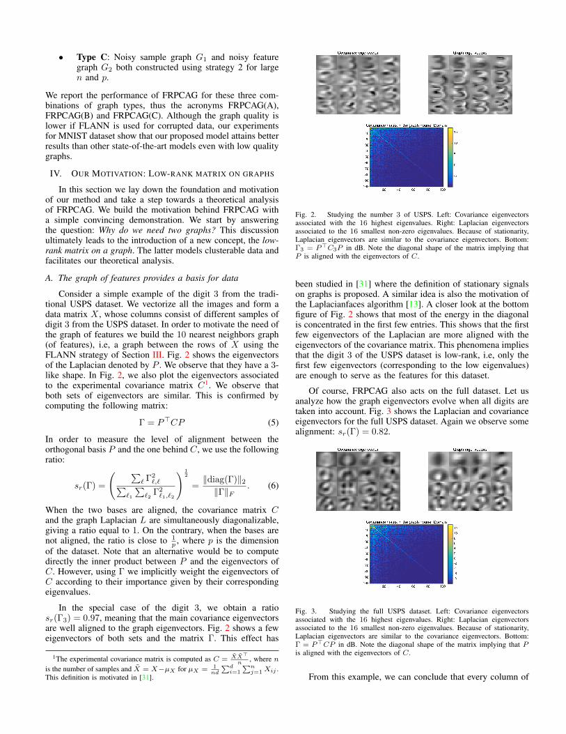
Consider a simple example of the digit 3 from the tradi-tional USPS dataset. We vectorize all the images and form adata matrix X , whose columns consist of different samples ofdigit 3 from the USPS dataset. In order to motivate the need ofthe graph of features we build the 10 nearest neighbors graph(of features), i.e, a graph between the rows of X using theFLANN strategy of Section III. Fig. 2 shows the eigenvectorsof the Laplacian denoted by P . We observe that they have a 3-like shape. In Fig. 2, we also plot the eigenvectors associatedto the experimental covariance matrix C1. We observe thatboth sets of eigenvectors are similar. This is confirmed bycomputing the following matrix:

Γ = P>CP (5)

In order to measure the level of alignment between theorthogonal basis P and the one behind C, we use the followingratio:

sr(Γ) =

( ∑` Γ2

`,`∑`1

∑`2

Γ2`1,`2

) 12

=‖diag(Γ)‖2‖Γ‖F

. (6)

When the two bases are aligned, the covariance matrix Cand the graph Laplacian L are simultaneously diagonalizable,giving a ratio equal to 1. On the contrary, when the bases arenot aligned, the ratio is close to 1

p , where p is the dimensionof the dataset. Note that an alternative would be to computedirectly the inner product between P and the eigenvectors ofC. However, using Γ we implicitly weight the eigenvectors ofC according to their importance given by their correspondingeigenvalues.

In the special case of the digit 3, we obtain a ratiosr(Γ3) = 0.97, meaning that the main covariance eigenvectorsare well aligned to the graph eigenvectors. Fig. 2 shows a feweigenvectors of both sets and the matrix Γ. This effect has

1The experimental covariance matrix is computed as C = XX>

n, where n

is the number of samples and X = X−µX for µX = 1nd

∑di=1

∑nj=1Xij .

This definition is motivated in [31].

Fig. 2. Studying the number 3 of USPS. Left: Covariance eigenvectorsassociated with the 16 highest eigenvalues. Right: Laplacian eigenvectorsassociated to the 16 smallest non-zero eigenvalues. Because of stationarity,Laplacian eigenvectors are similar to the covariance eigenvectors. Bottom:Γ3 = P>C3P in dB. Note the diagonal shape of the matrix implying thatP is aligned with the eigenvectors of C.

been studied in [31] where the definition of stationary signalson graphs is proposed. A similar idea is also the motivation ofthe Laplacianfaces algorithm [13]. A closer look at the bottomfigure of Fig. 2 shows that most of the energy in the diagonalis concentrated in the first few entries. This shows that the firstfew eigenvectors of the Laplacian are more aligned with theeigenvectors of the covariance matrix. This phenomena impliesthat the digit 3 of the USPS dataset is low-rank, i.e, only thefirst few eigenvectors (corresponding to the low eigenvalues)are enough to serve as the features for this dataset.

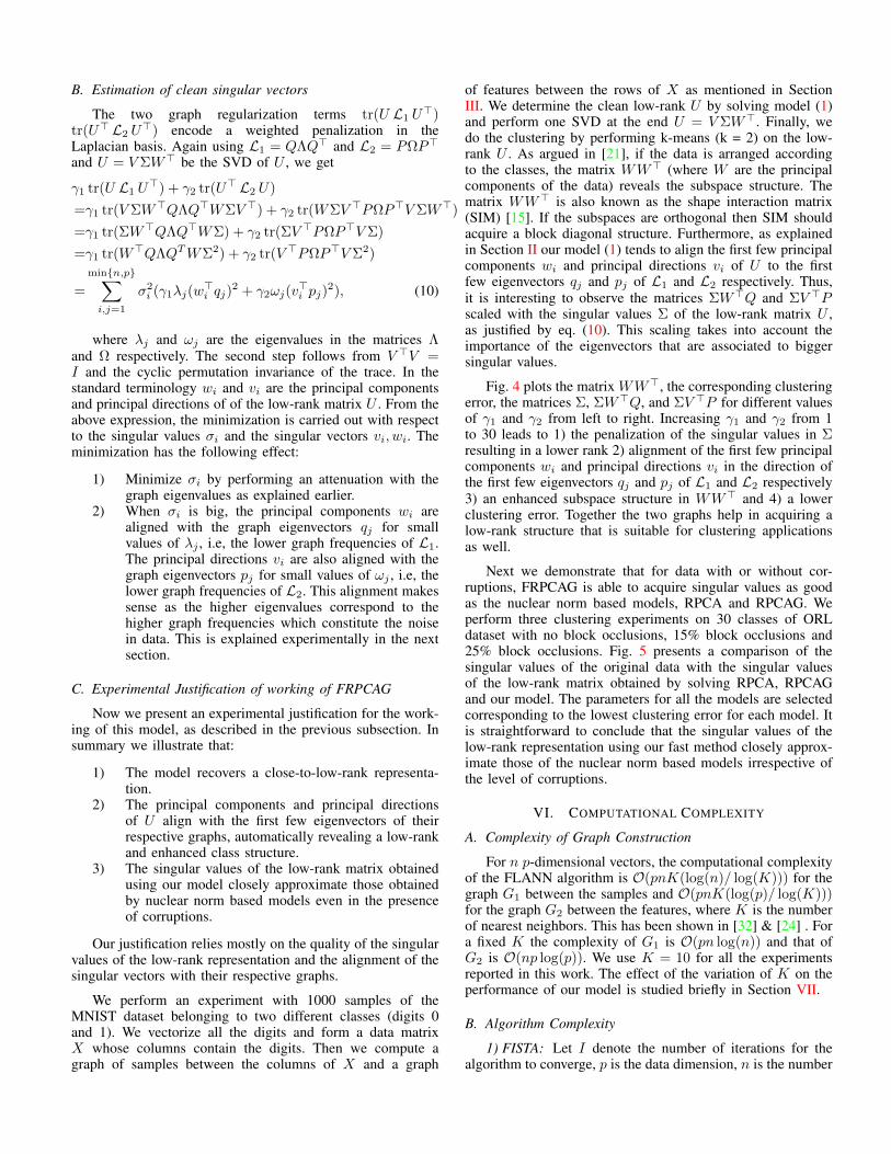
Of course, FRPCAG also acts on the full dataset. Let usanalyze how the graph eigenvectors evolve when all digits aretaken into account. Fig. 3 shows the Laplacian and covarianceeigenvectors for the full USPS dataset. Again we observe somealignment: sr(Γ) = 0.82.

Fig. 3. Studying the full USPS dataset. Left: Covariance eigenvectorsassociated with the 16 highest eigenvalues. Right: Laplacian eigenvectorsassociated to the 16 smallest non-zero eigenvalues. Because of stationarity,Laplacian eigenvectors are similar to the covariance eigenvectors. Bottom:Γ = P>CP in dB. Note the diagonal shape of the matrix implying that Pis aligned with the eigenvectors of C.

From this example, we can conclude that every column of

a low-rank matrix X lies approximately in the span of theeigenvectors Pk2 of the features graph, where k2 denotes theeigenvectors corresponding to the smallest k2 eigenvalues. Thisis similar to PCA, where a low-rank matrix is represented inthe span of the first few principal directions or atoms of thebasis. Alternately, the Laplacian eigenvectors are meaningfulfeatures for the USPS dataset. Let the eigenvectors P of L2

be divided into two sets (Pk2 ∈ Rp×k2 , Pk2 ∈ Rp×(p−k2)).Note that the columns of Pk2 contain the eigenvectors corre-sponding to the low graph frequencies and Pk2 contains thosecorresponding to higher graph frequencies. Then we can write,X = X∗ + E, where X∗ is the low-rank part and E modelsthe noise or corruptions. Thus,

X = Pk2A+ Pk2A and

X∗ = Pk2A

where A ∈ Rk2×n and A ∈ R(p−k2)×n. From Fig. 2 it is alsoclear that ‖Pk2A‖F ‖Pk2A‖F for a specific value of k2.

B. The graph of samples provides embedding for data

The smallest eigenvectors of the graph of samples providean embedding of the data in the low-dimensional space [4].This has a similar interpretation as the principal componentsin PCA. We argue that every row of a low-rank matrix liesin the span of the first few eigenvectors of the graph ofsamples. This is similar to representing every row of the low-rank matrix as the span of the principal components. Thus,the graph of samples L1 encodes a smooth non-linear maptowards the principal components of the underlying manifolddefined by the graph L1. In other words, minimization withrespect to tr(U L1 U

>) forces the principal components of thedata to be aligned with the eigenvectors Q of the graph L1

which correspond to the smallest eigenvalues λj . This is theheart of many algorithms in clustering [25] and dimensionalityreduction [4]. In our present application this term has twoeffects. Firstly, when the data has a class structure, the graphof samples enforces the low-rank U to benefit from this classstructure. This results in an enhanced clustering of the low-ranksignals. Secondly, it will force that the low-rank U of the sig-nals is well represented by the first few Laplacian eigenvectorsassociated to low λj . Let the eigenvectors Q of L1 be dividedinto two sets (Qk1 ∈ Rn×k1 , Qk1 ∈ Rn×(n−k1)), where k1denotes the eigenvectors in Q corresponding to the smallestk1 eigenvalues. Note that the columns of Qk1 contain theeigenvectors corresponding to the low graph frequencies andQk1 contains those corresponding to higher graph frequencies.Then, we can write:

X = BQ>k1 + BQ>k1 and

X∗ = BQ>k1

where B ∈ Rp×k1 and B ∈ Rp×(n−k1). As argued in theprevious subsection, ‖BQ>k1‖F ‖BQ>k1‖F .

C. Low-rank matrix on graphs

From the above explanation related to the role of thetwo graphs, we can conclude the following facts about therepresentation of any clusterable low-rank matrix X∗.

1) It can be represented as a linear combination of theLaplacian eigenvectors of the graph of features, i.e,X∗ = Pk2A.

2) It can also be represented as a linear combination ofthe Laplacian eigenvectors of the graph of samples,i.e, X∗ = BQ>k1 .

As already pointed out, only the first k1 or k2 eigenvectorsof the graphs correspond to the low frequency information,therefore, the other eigenvectors correspond to noise. We arenow in a position to define low-rank matrix on graphs.

Definition 1: A matrix X∗ is (k1, k2)-low-rank on thegraphs L1 and L2 if (X∗)>i ∈ span(Qk1) for all i = 1, . . . , p,and (X∗)j ∈ span(Pk2) for all j = 1, . . . , n. The set of(k1, k2)-low-rank matrices on the graphs L1 and L2 is denotedby LR(Qk1 , Pk2).

We note here that X∗ ∈ span(Pk2) means that the columnsof X∗ are in span(Pk2), i.e, (X∗)i ∈ span(Pk2), for all i =1, . . . , n, where for any matrix A, (A)i is its ith column vector.

D. Theoretical Analysis

The lower eigenvectors Qk1 and Pk2 of L1 and L2 providefeatures for any X ∈ LR(Qk1 , Pk2). Now we are readyto formalize our findings mathematically and prove that anysolution of (1) yields an approximately low-rank matrix. Infact, we prove this for any proper, positive, convex and lowersemi-continuous loss function φ (possibly `p-norms ‖·‖1, ‖·‖22,..., ‖ · ‖pp). We re-write (1) with a general loss function φ

minU

φ(U −X) + γ1 tr(U L1 U>) + γ2 tr(U> L2 U) (7)

Before presenting our mathematical analysis we gather afew facts which will be used later:

• We assume that the observed data matrix X satisfiesX = X∗ + E where X∗ ∈ LR(Qk1 , Pk2) and Emodels noise/corruptions. Furthermore, for any X∗ ∈LR(Qk1 , Pk2) there exists a matrix C such that X∗ =Pk2CQ

>k1

.

• L1 = QΛQ> = Qk1Λk1Q>k1

+ Qk1Λk1Q>k1

, whereΛk1 ∈ Rk1×k1 is a diagonal matrix of lower eigen-values and Λk1 ∈ R(n−k1)×(n−k1) is also a diagonalmatrix of higher graph eigenvalues. All values in Λare sorted in increasing order, thus 0 = λ0 ≤ λ1 ≤· · · ≤ λk1 ≤ · · · ≤ λn−1. The same holds for L2 aswell.

• For a K-nearest neighbors graph constructed from ak1-clusterable data (along samples) one can expectλk1/λk1+1 ≈ 0 as λk1 ≈ 0 and λk1 λk1+1. Thesame holds for the graph of features L2 as well.

• For the proof of the theorem, we will use the factthat for any X ∈ Rp×n, there exist A ∈ Rk2×n andA ∈ R(n−k2)×n such that X = Pk2A + Pk2A, andB ∈ Rp×k1 and B ∈ Rp×(n−k1) such that X =BQ>k1 + BQ>k1 .

Theorem 2: Let X∗ ∈ LR(Qk1 , Pk2), γ > 0, and E ∈Rp×n. Any solution U∗ ∈ Rp×n of (7) with γ1 = γ/λk1+1,

γ2 = γ/ωk2+1 and X = X∗ + E satisfies

φ(U∗ −X) + γ1‖U∗Qk1‖2F + γ2‖P>k2U∗‖2F≤ φ(E) + γ‖X∗‖2F

( λk1λk1+1

+ωk2ωk2+1

). (8)

where λk1 , λk1+1 denote the k1, k1 + 1 eigenvalues of L1,ωk2 , ωk2+1 denote the k2, k2 + 1 eigenvalues of L2.

Proof: As U∗ is a solution of (7), we have

φ(U∗ −X) + γ1 tr(U∗ L1(U∗)>) + γ2 tr((U∗)> L2 U∗)

≤ φ(E) + γ1 tr(X∗L1(X∗)>) + γ2 tr((X∗)> L2X∗). (9)

Using the facts that L1 = Qk1Λk1Q>k1

+ Qk1Λk1Q>k1

and thatthere exists B ∈ Rp×k1 and B ∈ Rp×(n−k1) such that U∗ =BQ>k1 + BQ>k1 , we obtain

tr(U∗ L1(U∗)>) = tr(BΛk1B>) + tr(BΛk1B

>)

≥ tr(Λk1B>B) ≥ λk1+1‖B‖2F = λk1+1‖U∗Qk1‖2F .

Then, using the fact that there exists C ∈ Rk2×k1 such thatX∗ = Pk2CQ

>k1

, we obtain

tr(X∗L1(X∗)>) = tr(CΛk1C>) ≤ λk1‖C‖2F = λk1‖X∗‖2F .

Similarly, we have

tr((U∗)> L2 U∗) ≥ ωk2+1‖P>k2U∗‖2F ,

tr((X∗)> L2X∗) ≤ ωk2‖X∗‖2F .

Using the four last bounds in (9) yields

φ(U∗ −X) + γ1λk1+1‖U∗Qk1‖2F + γ2ωk2+1‖P>k2U∗‖2F ≤φ(E) + γ1ωk1‖X∗‖2F + γ2ωk2‖X∗‖2F ,

which becomes

φ(U∗ −X) + γ‖U∗Qk1‖2F + γ‖P>k2U∗‖2F≤ φ(E) + γ‖X∗‖2F

(λk1λk1+1

+ωk2ωk2+1

)for our choice of γ1 and γ2. This terminates the proof.

E. Remarks on the theoretical analysis

(8) implies that

‖U∗Qk1‖2F + ‖P>k2U∗‖2F ≤1

γφ(E) + ‖X∗‖2F

(λk1λk1+1

+ωk2ωk2+1

).

The smaller ‖U∗Qk1‖2F + ‖P>k2U∗‖2F is, the closer U∗ toLR(Qk1 , Pk2) is. The above bound shows that to recover alow-rank matrix one should have large eigengaps λk1+1−λk1and ωk2+1 − ωk2 . This occurs when the rows and columns ofX can be clustered into k1 and k2 clusters. Furthermore, oneshould also try to chose a metric φ (or `p-norm) that minimizesφ(E). Clearly, the rank of U∗ is approximately mink1, k2.

V. WORKING OF FRPCAG

The previous section presented a theoretical analysis of ourmodel. In this section, we explain in detail the working ofour model for any data. Like any standard low-rank recoverymethod, such as [7], our method is able to perform thefollowing two operations for a clusterable data:

1) Penalization of the singular values of the data. Thepenalization of the higher singular values, whichcorrespond to high frequency components in the dataresults in the data cleaning.

2) Determination of the clean left and right singularvectors.

A. FRPCAG is a singular value penalization method

In order to demonstrate how FRPCAG penalizes the singu-lar values of the data we study another way to cater the graphregularization in the solution of the optimization problemwhich is contrary to the one presented in Section II-A. InSection II-A we used a gradient for the graph regularizationterms γ1 tr(U L1 U

>) + γ2 tr(U> L1 U) and used this gra-dient as an argument of the proximal operator for the soft-thresholding. What we did not point out there was that thesolution of the graph regularizations can also be computed byproximal operators. It is due to the reason that using proximaloperators for graph regularization (that we present here) ismore computationally expensive. Assume that the prox ofγ1 tr(U L1 U

>) is computed first, and let Z be a temporaryvariable, then it can be written as:

minZ‖X − Z‖2F + γ1 tr(Z L1 Z

>)

The above equation has a closed form solution which is givenas:

Z = X(I + γ1 L1)−1

Now, compute the proximal operator for the termγ2 tr(U> L2 U)

minU‖Z − U‖2F + γ2 tr(U> L2 U)

The closed form solution of the above equation is given as:

U = (I + γ2 L2)−1Z

Thus, the low-rank U can be written as:

U = (I + γ2 L2)−1X(I + γ1 L1)−1

after this the soft thresholding can be applied on U .

Let the SVD of X , X = VxΣxW>x , L1 = QΛQ> and

L2 = PΩP>, then we get:

U = (I + γ2PΛP>)−1VxΣxW>x (I + γ1QΩQ>)−1

= P (I + γ2Λ)−1P>VxΣxW>x Q(I + γ1Ω)−1Q>

thus, each singular value σxi of X is penalized by 1/(1 +γ1λi)(1 + γ2ωi). Clearly, the above solution requires thecomputation of two inverses which can be computationallyintractable for big datasets.

B. Estimation of clean singular vectors

The two graph regularization terms tr(U L1 U>)

tr(U> L2 U>) encode a weighted penalization in the

Laplacian basis. Again using L1 = QΛQ> and L2 = PΩP>

and U = V ΣW> be the SVD of U , we get

γ1 tr(U L1 U>) + γ2 tr(U> L2 U)

=γ1 tr(V ΣW>QΛQ>WΣV >) + γ2 tr(WΣV >PΩP>V ΣW>)

=γ1 tr(ΣW>QΛQ>WΣ) + γ2 tr(ΣV >PΩP>V Σ)

=γ1 tr(W>QΛQTWΣ2) + γ2 tr(V >PΩP>V Σ2)

=

minn,p∑i,j=1

σ2i (γ1λj(w

>i qj)

2 + γ2ωj(v>i pj)

2), (10)

where λj and ωj are the eigenvalues in the matrices Λand Ω respectively. The second step follows from V >V =I and the cyclic permutation invariance of the trace. In thestandard terminology wi and vi are the principal componentsand principal directions of of the low-rank matrix U . From theabove expression, the minimization is carried out with respectto the singular values σi and the singular vectors vi, wi. Theminimization has the following effect:

1) Minimize σi by performing an attenuation with thegraph eigenvalues as explained earlier.

2) When σi is big, the principal components wi arealigned with the graph eigenvectors qj for smallvalues of λj , i.e, the lower graph frequencies of L1.The principal directions vi are also aligned with thegraph eigenvectors pj for small values of ωj , i.e, thelower graph frequencies of L2. This alignment makessense as the higher eigenvalues correspond to thehigher graph frequencies which constitute the noisein data. This is explained experimentally in the nextsection.

C. Experimental Justification of working of FRPCAG

Now we present an experimental justification for the work-ing of this model, as described in the previous subsection. Insummary we illustrate that:

1) The model recovers a close-to-low-rank representa-tion.

2) The principal components and principal directionsof U align with the first few eigenvectors of theirrespective graphs, automatically revealing a low-rankand enhanced class structure.

3) The singular values of the low-rank matrix obtainedusing our model closely approximate those obtainedby nuclear norm based models even in the presenceof corruptions.

Our justification relies mostly on the quality of the singularvalues of the low-rank representation and the alignment of thesingular vectors with their respective graphs.

We perform an experiment with 1000 samples of theMNIST dataset belonging to two different classes (digits 0and 1). We vectorize all the digits and form a data matrixX whose columns contain the digits. Then we compute agraph of samples between the columns of X and a graph

of features between the rows of X as mentioned in SectionIII. We determine the clean low-rank U by solving model (1)and perform one SVD at the end U = V ΣW>. Finally, wedo the clustering by performing k-means (k = 2) on the low-rank U . As argued in [21], if the data is arranged accordingto the classes, the matrix WW> (where W are the principalcomponents of the data) reveals the subspace structure. Thematrix WW> is also known as the shape interaction matrix(SIM) [15]. If the subspaces are orthogonal then SIM shouldacquire a block diagonal structure. Furthermore, as explainedin Section II our model (1) tends to align the first few principalcomponents wi and principal directions vi of U to the firstfew eigenvectors qj and pj of L1 and L2 respectively. Thus,it is interesting to observe the matrices ΣW>Q and ΣV >Pscaled with the singular values Σ of the low-rank matrix U ,as justified by eq. (10). This scaling takes into account theimportance of the eigenvectors that are associated to biggersingular values.

Fig. 4 plots the matrix WW>, the corresponding clusteringerror, the matrices Σ, ΣW>Q, and ΣV >P for different valuesof γ1 and γ2 from left to right. Increasing γ1 and γ2 from 1to 30 leads to 1) the penalization of the singular values in Σresulting in a lower rank 2) alignment of the first few principalcomponents wi and principal directions vi in the direction ofthe first few eigenvectors qj and pj of L1 and L2 respectively3) an enhanced subspace structure in WW> and 4) a lowerclustering error. Together the two graphs help in acquiring alow-rank structure that is suitable for clustering applicationsas well.

Next we demonstrate that for data with or without cor-ruptions, FRPCAG is able to acquire singular values as goodas the nuclear norm based models, RPCA and RPCAG. Weperform three clustering experiments on 30 classes of ORLdataset with no block occlusions, 15% block occlusions and25% block occlusions. Fig. 5 presents a comparison of thesingular values of the original data with the singular valuesof the low-rank matrix obtained by solving RPCA, RPCAGand our model. The parameters for all the models are selectedcorresponding to the lowest clustering error for each model. Itis straightforward to conclude that the singular values of thelow-rank representation using our fast method closely approx-imate those of the nuclear norm based models irrespective ofthe level of corruptions.

VI. COMPUTATIONAL COMPLEXITY

A. Complexity of Graph Construction

For n p-dimensional vectors, the computational complexityof the FLANN algorithm is O(pnK(log(n)/ log(K))) for thegraph G1 between the samples and O(pnK(log(p)/ log(K)))for the graph G2 between the features, where K is the numberof nearest neighbors. This has been shown in [32] & [24] . Fora fixed K the complexity of G1 is O(pn log(n)) and that ofG2 is O(np log(p)). We use K = 10 for all the experimentsreported in this work. The effect of the variation of K on theperformance of our model is studied briefly in Section VII.

B. Algorithm Complexity

1) FISTA: Let I denote the number of iterations for thealgorithm to converge, p is the data dimension, n is the number

WW> WW> WW>

0.1max 0.1max 0.1max

Fig. 4. The matrices WW>, Σ, ΣW>Q, ΣV >P and the corresponding clustering errors obtained for different values of the weights on the two graphregularization terms for 1000 samples of MNIST dataset (digits 0 and 1). If U = V ΣW> is the SVD of U , then W corresponds to the matrix of principalcomponents (right singular vectors of U ) and V to the principal directions (left singular vectors of U ). Let L1 = QΛQ> and L2 = PΩP> be the eigenvaluedecompositions of L1 and L2 respectively then Q and P correspond to the eigenvectors of Laplacians L1 and L2. The block diagonal structure of WW>

becomes more clear by increasing γ1 and γ2 with a thresholding of the singular values in Σ. Further, the sparse structures of ΣW>Q and ΣV >P towardsthe rightmost corners show that the number of left and right singular vectors which align with the eigenvectors of the Laplacians L1 and L2 go on decreasingwith increasing γ1 and γ2. This shows that the two graphs help in attaining a low-rank structure with a low clustering error.

Fig. 5. A comparison of singular values of the low-rank matrix obtained via our model, RPCA and RPCAG. The experiments were performed on the ORLdataset with different levels of block occlusions. The parameters corresponding to the minimum validation clustering error for each of the model were used.

of samples and c is the rank of the low-dimensional space. Thecomputational cost of our algorithm per iteration is linear inthe number of data samples n, i.e. O(Ipn) for I iterations.

2) Final SVD: Our model, in order to preserve convexity,finds an approximately low-rank solution U without explicitlyfactorizing it. While this gives a great advantage, dependingon the application we have in hand, we might need to provideexplicitly the low dimensional representation in a factorizedform. This can be done by computing an “economic” SVD ofU after our algorithm has finished.

Most importantly, this computation can be done in timethat scales linearly with the number of samples for a fixednumber of features p n. Let U = V ΣW> the SVD of U .The orthonormal basis V can be computed by the eigenvaluedecomposition of the small p× p matrix UU> = V EV > thatalso reveals the singular values Σ =

√E since UU> is s.p.s.d.

and therefore E is non-negative diagonal. Here we chooseto keep only the c biggest singular values and correspondingvectors according to the application in hand (the procedure fordetermining c is explained in Section VII). Given V and Σ thesample projections are computed as W = Σ−1V >U .

The complexity of this SVD is O(np2) –due to the multi-plication UU>– and does not change the asymptotic complex-ity of our algorithm. Note that the standard economic SVDimplementation in numerical analysis software typically doesnot use this simple trick, in order to achieve better numericalerror. However, in most machine learning applications like theones of interest in this paper, the compromise in terms ofnumerical error is negligible compared to the gains in termsof scalability.

C. Overall Complexity

The complexity of FISTA is O(Ipn), the graph G1 isO(pn log(n)), G2 is O(pn log(p)) and the final SVD step isO(np2). Given that p n, the overall complexity of ouralgorithm is O(pn(log(n)+I+p+log(p))). Table II presentsthe computational complexities of all the models consideredin this work (discussed in Section VII).

D. Scalability

The construction of graphs G1 and G2 is highly scalable.For small n and p the strategy 1 of Section III can be usedfor the graphs construction and each of the entries of theadjacency matrix A can be computed in parallel once thenearest neighbors have been found. For large n an p theapproximate K-nearest neighbors scheme (FLANN) is usedfor graphs construction which is highly scalable as well. Next,our proposed FISTA algorithm for FRPCAG requires twoimportant computations at every iteration: 1) computation ofproximal operator proxλh(U) and 2) the gradient ∇g(Y ).The former computation is given by the element-wise soft-thresholding (eq. (4)) that can be performed in parallel forall the entries of a matrix. The gradient computation, asgiven by eq. (3), involves matrix-matrix multiplications thatinvolve sparse matrices L1 and L2 and can be performed veryefficiently in parallel as well.

VII. RESULTS

Experiments were done using two open-source toolboxes:the UNLocBoX [30] for the optimization part and the GSPBox[29] for the graph creation. The complete demo, code anddatasets used for this work are available at . We performtwo types of experiments corresponding to two applicationsof PCA.

1) Data clustering in the low-dimensional space.2) Low-rank recovery: Static background separation

from videos.

We present extensive quantitative results for clustering butcurrently our experiments for low-rank recovery are limitedto qualitative analysis only. This is because our work onapproximating the low-rank representation using graphs is thefirst of its kind. The experiments on the low-rank backgroundextraction from videos suffice as a proof-of-concept for theworking of this model.

We perform our clustering experiments on 7 benchmarkdatabases: CMU PIE, ORL, YALE, COIL20, MNIST, USPSand MFEAT. CMU PIE, ORL and YALE are face databaseswith small pose variations. COIL20 is a dataset of objectswith significant pose changes so we select the images for

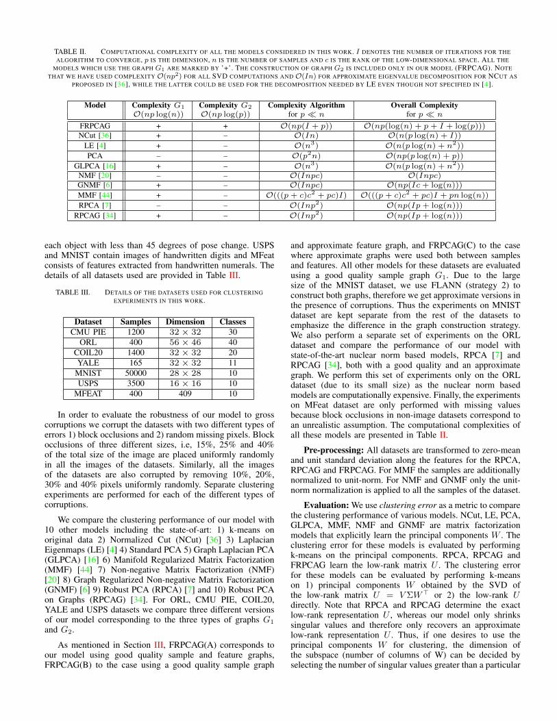
TABLE II. COMPUTATIONAL COMPLEXITY OF ALL THE MODELS CONSIDERED IN THIS WORK. I DENOTES THE NUMBER OF ITERATIONS FOR THEALGORITHM TO CONVERGE, p IS THE DIMENSION, n IS THE NUMBER OF SAMPLES AND c IS THE RANK OF THE LOW-DIMENSIONAL SPACE. ALL THE

MODELS WHICH USE THE GRAPH G1 ARE MARKED BY ’+’. THE CONSTRUCTION OF GRAPH G2 IS INCLUDED ONLY IN OUR MODEL (FRPCAG). NOTETHAT WE HAVE USED COMPLEXITY O(np2) FOR ALL SVD COMPUTATIONS AND O(In) FOR APPROXIMATE EIGENVALUE DECOMPOSITION FOR NCUT AS

PROPOSED IN [36], WHILE THE LATTER COULD BE USED FOR THE DECOMPOSITION NEEDED BY LE EVEN THOUGH NOT SPECIFIED IN [4].

Model Complexity G1 Complexity G2 Complexity Algorithm Overall ComplexityO(np log(n)) O(np log(p)) for p n for p n

FRPCAG + + O(np(I + p)) O(np(log(n) + p+ I + log(p)))NCut [36] + – O(In) O(n(p log(n) + I))

LE [4] + – O(n3) O(n(p log(n) + n2))

PCA – – O(p2n) O(np(p log(n) + p))

GLPCA [16] + – O(n3) O(n(p log(n) + n2))NMF [20] – – O(Inpc) O(Inpc)GNMF [6] + – O(Inpc) O(np(Ic+ log(n)))

MMF [44] + – O(((p+ c)c2 + pc)I) O(((p+ c)c2 + pc)I + pn log(n))

RPCA [7] – – O(Inp2) O(np(Ip+ log(n)))

RPCAG [34] + – O(Inp2) O(np(Ip+ log(n)))

each object with less than 45 degrees of pose change. USPSand MNIST contain images of handwritten digits and MFeatconsists of features extracted from handwritten numerals. Thedetails of all datasets used are provided in Table III.

TABLE III. DETAILS OF THE DATASETS USED FOR CLUSTERINGEXPERIMENTS IN THIS WORK.

Dataset Samples Dimension ClassesCMU PIE 1200 32× 32 30

ORL 400 56× 46 40COIL20 1400 32× 32 20YALE 165 32× 32 11

MNIST 50000 28× 28 10USPS 3500 16× 16 10

MFEAT 400 409 10

In order to evaluate the robustness of our model to grosscorruptions we corrupt the datasets with two different types oferrors 1) block occlusions and 2) random missing pixels. Blockocclusions of three different sizes, i.e, 15%, 25% and 40%of the total size of the image are placed uniformly randomlyin all the images of the datasets. Similarly, all the imagesof the datasets are also corrupted by removing 10%, 20%,30% and 40% pixels uniformly randomly. Separate clusteringexperiments are performed for each of the different types ofcorruptions.

We compare the clustering performance of our model with10 other models including the state-of-art: 1) k-means onoriginal data 2) Normalized Cut (NCut) [36] 3) LaplacianEigenmaps (LE) [4] 4) Standard PCA 5) Graph Laplacian PCA(GLPCA) [16] 6) Manifold Regularized Matrix Factorization(MMF) [44] 7) Non-negative Matrix Factorization (NMF)[20] 8) Graph Regularized Non-negative Matrix Factorization(GNMF) [6] 9) Robust PCA (RPCA) [7] and 10) Robust PCAon Graphs (RPCAG) [34]. For ORL, CMU PIE, COIL20,YALE and USPS datasets we compare three different versionsof our model corresponding to the three types of graphs G1

and G2.

As mentioned in Section III, FRPCAG(A) corresponds toour model using good quality sample and feature graphs,FRPCAG(B) to the case using a good quality sample graph

and approximate feature graph, and FRPCAG(C) to the casewhere approximate graphs were used both between samplesand features. All other models for these datasets are evaluatedusing a good quality sample graph G1. Due to the largesize of the MNIST dataset, we use FLANN (strategy 2) toconstruct both graphs, therefore we get approximate versions inthe presence of corruptions. Thus the experiments on MNISTdataset are kept separate from the rest of the datasets toemphasize the difference in the graph construction strategy.We also perform a separate set of experiments on the ORLdataset and compare the performance of our model withstate-of-the-art nuclear norm based models, RPCA [7] andRPCAG [34], both with a good quality and an approximategraph. We perform this set of experiments only on the ORLdataset (due to its small size) as the nuclear norm basedmodels are computationally expensive. Finally, the experimentson MFeat dataset are only performed with missing valuesbecause block occlusions in non-image datasets correspond toan unrealistic assumption. The computational complexities ofall these models are presented in Table II.

Pre-processing: All datasets are transformed to zero-meanand unit standard deviation along the features for the RPCA,RPCAG and FRPCAG. For MMF the samples are additionallynormalized to unit-norm. For NMF and GNMF only the unit-norm normalization is applied to all the samples of the dataset.

Evaluation: We use clustering error as a metric to comparethe clustering performance of various models. NCut, LE, PCA,GLPCA, MMF, NMF and GNMF are matrix factorizationmodels that explicitly learn the principal components W . Theclustering error for these models is evaluated by performingk-means on the principal components. RPCA, RPCAG andFRPCAG learn the low-rank matrix U . The clustering errorfor these models can be evaluated by performing k-meanson 1) principal components W obtained by the SVD ofthe low-rank matrix U = V ΣW> or 2) the low-rank Udirectly. Note that RPCA and RPCAG determine the exactlow-rank representation U , whereas our model only shrinkssingular values and therefore only recovers an approximatelow-rank representation U . Thus, if one desires to use theprincipal components W for clustering, the dimension ofthe subspace (number of columns of W) can be decided byselecting the number of singular values greater than a particular

threshold. However, this procedure requires SVD and canbe expensive for big datasets. Instead, it is more feasible toperform clustering on the low-rank U directly. We observedthat similar clustering results are obtained by using either Wor U , however, for brevity these results are not reported. Dueto the non-deterministic nature of k-means, it is run 10 timesand the minimum error over all runs is reported.

Parameter selection for various models: Each model hasseveral parameters which have to be selected in the validationstage of the experiment. To perform a fair validation for eachof the models we use a range of parameter values as presentedin Table IV. For a given dataset, each of the models is run foreach of the parameter tuples in this table and the parameterscorresponding to minimum clustering error are selected fortesting purpose. Furthermore, PCA, GLPCA, MMF, NMF andGNMF are non-convex models so they are run 10 times foreach of the parameter tuple. RPCA, RPCAG and FRPCAG areconvex so they are run only once.

TABLE IV. RANGE OF PARAMETER VALUES FOR EACH OF THEMODELS CONSIDERED IN THIS WORK. c IS THE RANK OR DIMENSION OFSUBSPACE, λ IS THE WEIGHT ASSOCIATED WITH THE SPARSE TERM FORROBUST PCA FRAMEWORK [7] AND γ IS THE PARAMETER ASSOCIATED

WITH THE GRAPH REGULARIZATION TERM.

Model Para- Parametermeters Range

NCut [36]LE [4] c c ∈ 21, 22, · · · ,min(n, p)PCA

GLPCA [16] c ∈ 21, 22, · · · ,min(n, p)c, γ γ =⇒ β using [16]

β ∈ 0.1, 0.2, · · · , 0.9MMF [44] c, γ c ∈ 21, 22, · · · ,min(n, p)NMF [20] cGNMF [6] c, γ γ ∈ 2−3, 2−2, · · · , 210RPCA [7] λ λ ∈ 2−3√

max(n,p):

0.1 : 23√max(n,p)

RPCAG [34] λ, γ γ ∈ 2−3, 2−2, · · · , 210

FRPCAG γ1, γ2 γ1, γ2 ∈ 1, 2, · · · , 100

Parameter selection for Graphs: For all the experimentsreported in this paper we use the following parameters forgraphs G1 and G2. K-nearest neighbors = 10 and σ2 = 1. It isimportant to point out here that different types of data mightcall for slightly different parameters for graphs. However, for agiven dataset, the use of same graph parameters (same graphquality) for all the graph regularized models ensures a faircomparison.

A. Clustering

1) Comparison with Matrix Factorization Models: Fig. 6presents the clustering error for various matrix factorizationand our proposed model. NMF and GNMF are not evaluatedfor the USPS and MFeat datasets as they are not originally non-negative. It can be seen that our proposed model FRPCAG(A)with the two good quality graphs performs better than allthe other models in most of the cases both in the presenceand absence of data corruptions. Even FRPCAG(B) with agood sample graph G1 and a noisy feature graph G2 performs

reasonably well. This shows that our model is quite robust tothe quality of graph G2. However, as expected FRPCAG(C)performs worse for ORL, CMU PIE, COIL20, YALE andUSPS datasets as compared to other models evaluated with agood sample graph G1. Finally, our model outperforms othersin most of the cases for the interesting case of MNIST datasetwhere both graphs G1 and G2 are noisy for all models underconsideration. It is worth mentioning here that even thoughthe absolute errors are quite high for FRPCAG on the MNISTdataset, it performs relatively better than the other models.As PCA is mostly used as a feature extraction or a pre-processing step for a variety of machine learning algorithms, abetter absolute classification performance can be obtained forthese datasets by using FRPCAG as a pre-processing step forsupervised algorithms as compared to other PCA models.

2) Comparison with Nuclear Norm based Models: Fig. 6also presents a comparison of the clustering error of our modelwith nuclear norm based models, i.e, RPCA and RPCAG forORL dataset. This comparison is of specific interest becauseof the convexity of all the algorithms under consideration. Asthese models require an expensive SVD step on the wholelow-rank matrix at every iteration of the algorithm, theseexperiments are performed on small ORL dataset. Clearly, ourproposed model FRPCAG(A) performs better than the nuclearnorm based models even in the presence of large fractionof gross errors. Interestingly, even FRPCAG(B) with a noisygraph G2 performs better than RPCAG with a good graph G1.Furthermore, the performance of FRPCAG(C) with two noisygraphs is comparable to RPCAG with noisy graph, but stillbetter than RPCA.

B. Principal Components

Fig. 7 shows the principal components of 1000 samples ofMNIST dataset in two dimensional space obtained by variousdimensionality reduction models. 500 samples of digit 0 and1 each are chosen and randomly corrupted by 15% missingpixels for this experiment. Clearly, our proposed model attainsa good separation between the digits 0 and 1 (represented byblue and red points respectively) comparable with other state-of-the-art dimensionality reduction models.

C. Effect of the number of nearest neighbors for graphs

In order to demonstrate the effect of number of nearestneighbors K on the clustering performance of our model weperform a small experiment on the ORL dataset which has 400images corresponding to 40 classes (10 images per class). Weperform clustering for different values of K = 5, 10, 25, 40.The clustering errors are 17.5%, 17%, 23% and 31% respec-tively. Interestingly the minimum clustering error occurs forK = 5, 10 which is less or equal to the number of imagesper class. Thus, when the number of nearest neighbors K isapproximately equal to or less than the number of imagesper class then the images of the same class are more wellconnected and those across the classes have weak connections.This results in a lower clustering error. A good way to set Kis to use some prior information about the average numberof samples per class or the rank of the dataset. For ourexperiments we use K = 10 for all the datasets and this valueworks quite well. The value of K also depends on the numberof data samples. For big datasets, sparser graphs (obtained

No Corruptions

Corruptions on the dataset Occlusions (% of image size) Missing values (% of image size)

15% 25% 40% 10% 20% 30% 40%

% Clustering Error of various models

No experiments with block occlusionsbecause it is a non-image dataset

Fig. 6. A comparison of clustering error of our model with various dimensionality reduction models. The image data sets include: 1) ORL 2) CMU PIE 3)COIL20 and 4) YALE. The compared models are: 1) k-means 2) Normalized Cut (NCut) 3) Laplacian Eigenmaps (LE) [4] 4) Standard Principal ComponentAnalysis (PCA) 5) Graph Laplacian PCA (GLPCA) [16] 6) Non-negative Matrix Factorization [20] 7) Graph Regularized Non-negative Matrix Factorization(GNMF) [6] 8) Manifold Regularized Matrix Factorization (MMF) [44] 9) Robust PCA (RPCA) [7] 10) Fast Robust PCA on Graphs (A) 11) Fast Robust PCAon Graphs (B) and 12) Fast Robust PCA on Graphs (C). Two types of corruptions are introduced in the data: 1) Block occlusions and 2) Random missingvalues. NCut, LE, GLPCA, MMF and GNMF are evaluated with a good sample graph G1. FRPCA(A) corresponds to our model evaluated with a good sampleand a good feature graph, FRPCA(B) to a good sample graph and a noisy feature graph and FRPCA(C) to a noisy sample and feature graph. NMF and GNMFrequire non-negative data so they were not evaluated for the USPS and MFeat datasets because they are negative as well. MFeat is a non-image dataset so it isnot evaluated with block occlusions. Due to the large size of the MNIST dataset, we use FLANN algorithm (strategy 2) to construct the graphs, therefore weget noisy graphs in the presence of corruptions.

Fig. 7. Principal Components of 1000 samples of digits 0 and 1 of the MNIST dataset in 2D space. For this experiment all the digits were corrupted randomlywith 15% missing pixels. Our proposed model (lower right) attains a good separation between the digits which is comparable and even better than otherstate-of-the-art dimensionality reduction models.

Original RPCA RPCAG FRPCAGBackground Separation from Videos via PCA

Fig. 8. Static background separation from three videos. Each row shows the actual frame (left), recovered static low-rank background using RPCA, RPCAGand our proposed model. The first row corresponds to the video of a restaurant food counter, the second row to the shopping mall lobby and the third to anairport lobby. In all the three videos the moving people belong to the sparse component. Thus, our model is able to accurately separate the static portion fromthe three frames as good as the RPCAG. Our model converged in less than 2 minutes for each of the three videos, whereas RPCA and RPCAG converged inmore than 45 minutes.

with lower values of K) tend to be more useful. For example,our experiments show that for the MNIST dataset (70,000samples), K = 10 is again a good value, even though theaverage number of samples per class is 7000.

D. Static background separation from videos

In order to demonstrate the effectiveness of our model torecover low-rank static background from videos we performexperiments on 1000 frames of 3 videos available online. Allthe frames are vectorized and arranged in a matrix X whosecolumns correspond to frames. The graph G1 is constructedbetween the 1000 frames (columns of X) of the video and thegraph G2 is constructed between the pixels of the frames (rowsof X) following the methodology of Section III. Both graphsfor all the videos are constructed without the prior knowledgeof the mask of sparse errors (moving people). Fig. 8 shows therecovery of low-rank frames for one actual frame of each of thevideos. The leftmost plot in each row shows the actual frame,the other three show the recovered low-rank representationsusing RPCA, RPCAG and our proposed model (FRPCAG).The first row corresponds to a frame from the video of arestaurant food counter, the second row to the shopping malllobby and the third row to an airport lobby. In each of thethree plots it can be seen that our proposed model is ableto separate the static backgrounds very accurately from themoving people which do not belong to the static ground truth.Our model converged in less than 2 minutes for each of thethree videos, whereas RPCA and RPCAG converged in morethan 45 minutes.

E. Computational Time

Table V presents the computational time and numberof iterations for the convergence of FRPCAG, RPCAG andRPCA on different sizes and dimensions of the datasets. Wealso present the time needed for the graph construction. Thecomputation is done on a single core machine with a 3.3 GHzprocessor without using any distributed or parallel computingtricks. An ∞ in the table indicates that the algorithm did notconverge in 4 hours. It is notable that our model requires a verysmall number of iterations to converge irrespective of the sizeof the dataset. Furthermore, the model is orders of magnitudefaster than RPCA and RPCAG. This is clearly observed fromthe experiments on MNIST dataset where our proposed modelis 100 times faster than RPCAG. Specially for MNIST datasetwith 25000 samples, RPCAG and RPCA did not converge evenin 4 hours whereas FRPCAG converged in less than a minute.

To demonstrate the scalability of our model for big datasets,we perform an experiment on the US census 1990 datasetavailable at the UCI machine learning repository. This datasetconsists of approximately 2.5 million samples and 68 fea-tures. The approximate K-nearest neighbors graph constructionstrategy using the FLANN algorithm took only 540 secs toconstruct G1 between 2.5 million samples and 42.3 secs. toconstruct G2 between 68 features. We do not compare theperformance of this model with other state-of-the-art modelsas the ground truth for this dataset is not available. However,we run our algorithm in order to see how long it takes torecover a low-rank representation for this dataset. It took 65minutes and 200 iterations for the algorithm to converge on asingle core machine with 3.3 GHz of CPU power.

VIII. CONCLUSION

We present Fast Robust PCA on Graphs (FRPCAG), a fastdimensionality reduction algorithm for mining clusters fromhigh dimensional and large low-rank datasets. The idea lieson the novel concept of low-rank matrices on graphs. Thepower of the model lies in its ability to effectively exploitthe hidden information about the intrinsic dimensionality ofthe smooth low-dimensional manifolds on which reside theclusterable signals and features of the data. Therefore, it targetsan approximate recovery of low-rank signals by exploiting thelocal smoothness assumption of the samples and features of thedata via graph structures only. In short our method leverages 1)smoothness of the samples on a sample graph and 2) smooth-ness of the features on a feature graph. The proposed methodis convex, scalable and efficient and tends to outperformseveral other state-of-the-art exact low-rank recovery methodsin clustering tasks that use the expensive nuclear norm. In anordinary clustering task FRPCAG is approximately 100 timesfaster than nuclear norm based methods. The double graphstructure also plays an important role towards the robustnessof the model to gross corruptions. Furthermore, the singularvalues of the low-rank matrix obtained via FRPCAG closelyapproximate those obtained via nuclear norm based methods.

ACKNOWLEDGEMENT

The work of Nauman Shahid and Nathanael Perraudin issupported by the SNF grant no. 200021 154350/1 for theproject “Towards signal processing on graphs”. The work ofG. Puy is funded by the FP7 European Research CouncilProgramme, PLEASE project, under grant ERC-StG-2011-277906. We would also like to thank Benjamin Ricaud forhis valuable suggestions to improve the paper.

REFERENCES

[1] H. Abdi and L. J. Williams. Principal component analysis. WileyInterdisciplinary Reviews: Computational Statistics, 2(4):433–459,2010. 1

[2] M. Ayazoglu, M. Sznaier, O. Camps, et al. Fast algorithms for structuredrobust principal component analysis. In Computer Vision and PatternRecognition (CVPR), 2012 IEEE Conference on, pages 1704–1711.IEEE, 2012. 2

[3] A. Beck and M. Teboulle. A fast iterative shrinkage-thresholdingalgorithm for linear inverse problems. SIAM Journal on ImagingSciences, 2(1):183–202, 2009. 4

[4] M. Belkin and P. Niyogi. Laplacian eigenmaps for dimensionalityreduction and data representation. Neural computation, 15(6):1373–1396, 2003. 2, 6, 11, 12, 13

[5] K. Benzi, V. Kalofolias, X. Bresson, and P. Vandergheynst. SongRecommendation with Non-Negative Matrix Factorization and GraphTotal Variation, Jan. 2016. 3

[6] D. Cai, X. He, J. Han, and T. S. Huang. Graph regularized nonnegativematrix factorization for data representation. Pattern Analysis andMachine Intelligence, IEEE Transactions on, 33(8):1548–1560, 2011.2, 11, 12, 13

[7] E. J. Candes, X. Li, Y. Ma, and J. Wright. Robust principal componentanalysis? Journal of the ACM (JACM), 58(3):11, 2011. 2, 7, 11, 12,13

[8] P. L. Combettes and J.-C. Pesquet. Proximal splitting methods in signalprocessing. In Fixed-point algorithms for inverse problems in scienceand engineering, pages 185–212. Springer, 2011. 4

[9] H. Du, X. Zhang, Q. Hu, and Y. Hou. Sparse representation-based robustface recognition by graph regularized low-rank sparse representationrecovery. Neurocomputing, 164:220–229, 2015. 2

[10] E. Elhamifar and R. Vidal. Sparse subspace clustering: Algorithm,theory, and applications. Pattern Analysis and Machine Intelligence,IEEE Transactions on, 35(11):2765–2781, 2013. 1

TABLE V. COMPUTATION TIMES (IN SECONDS) FOR GRAPHS G1 , G2 , FRPCAG, RPCAG, RPCA AND THE NUMBER OF ITERATIONS TO CONVERGEFOR DIFFERENT DATASETS. THE COMPUTATION IS DONE ON A SINGLE CORE MACHINE WITH A 3.3 GHZ PROCESSOR WITHOUT USING ANY DISTRIBUTED

OR PARALLEL COMPUTING TRICKS.∞ INDICATES THAT THE ALGORITHM DID NOT CONVERGE IN 4 HOURS.

Dataset Samples Features Classes Graphs FRPCAG RPCAG RPCAG1 G2 time Iters time Iters time Iters

MNIST 5000 784 10 10.8 4.3 13.7 27 1345 325 1090 378MNIST 15000 784 10 32.5 13.3 35.4 23 3801 412 3400 323MNIST 25000 784 10 40.7 22.2 58.6 24 ∞ ∞ ∞ ∞

ORL 300 10304 30 1.8 56.4 4.7 12 360 301 240 320USPS 3500 256 10 5.8 10.8 1.76 16 900 410 790 350

US census 2.5 million 68 - 540 42.3 3900 200 ∞ ∞ ∞ ∞

[11] S. Gao, I.-H. Tsang, and L.-T. Chia. Laplacian sparse coding, hyper-graph laplacian sparse coding, and applications. Pattern Analysis andMachine Intelligence, IEEE Transactions on, 35(1):92–104, 2013. 2

[12] Q. Gu and J. Zhou. Co-clustering on manifolds. In Proceedings of the15th ACM SIGKDD international conference on Knowledge discoveryand data mining, pages 359–368. ACM, 2009. 3

[13] X. He, S. Yan, Y. Hu, P. Niyogi, and H.-J. Zhang. Face recognitionusing laplacianfaces. Pattern Analysis and Machine Intelligence, IEEETransactions on, 27(3):328–340, 2005. 5

[14] R. Jenatton, G. Obozinski, and F. Bach. Structured sparse principalcomponent analysis. arXiv preprint arXiv:0909.1440, 2009. 2

[15] P. Ji, M. Salzmann, and H. Li. Shape interaction matrix revisited androbustified: Efficient subspace clustering with corrupted and incompletedata. In Proceedings of the IEEE International Conference on ComputerVision, pages 4687–4695, 2015. 8

[16] B. Jiang, C. Ding, and J. Tang. Graph-laplacian pca: Closed-formsolution and robustness. In Computer Vision and Pattern Recognition(CVPR), 2013 IEEE Conference on, pages 3492–3498. IEEE, 2013. 2,11, 12, 13

[17] T. Jin, J. Yu, J. You, K. Zeng, C. Li, and Z. Yu. Low-rank matrix fac-torization with multiple hypergraph regularizers. Pattern Recognition,2014. 2

[18] T. Jin, Z. Yu, L. Li, and C. Li. Multiple graph regularized sparsecoding and multiple hypergraph regularized sparse coding for imagerepresentation. Neurocomputing, 2014. 2

[19] V. Kalofolias, X. Bresson, M. Bronstein, and P. Vandergheynst. Matrixcompletion on graphs. arXiv preprint arXiv:1408.1717, 2014. 3

[20] D. D. Lee and H. S. Seung. Learning the parts of objects by non-negative matrix factorization. Nature, 401(6755):788–791, 1999. 1, 11,12, 13

[21] G. Liu, Z. Lin, S. Yan, J. Sun, Y. Yu, and Y. Ma. Robust recovery ofsubspace structures by low-rank representation. Pattern Analysis andMachine Intelligence, IEEE Transactions on, 35(1):171–184, 2013. 1,8

[22] A. Lucas, M. Stalzer, and J. Feo. Parallel implementation of fastrandomized algorithms for low rank matrix decomposition. ParallelProcessing Letters, 24(01), 2014. 2

[23] J. Mairal, F. Bach, and J. Ponce. Sparse modeling for image and visionprocessing. arXiv preprint arXiv:1411.3230, 2014. 2

[24] M. Muja and D. Lowe. Scalable nearest neighbour algorithms for highdimensional data. 2014. 4, 8

[25] A. Y. Ng, M. I. Jordan, Y. Weiss, et al. On spectral clustering: Analysisand an algorithm. Advances in neural information processing systems,2:849–856, 2002. 6

[26] T.-H. Oh, Y. Matsushita, Y.-W. Tai, and I. S. Kweon. Fast random-ized singular value thresholding for nuclear norm minimization. InProceedings of the IEEE Conference on Computer Vision and PatternRecognition, pages 4484–4493, 2015. 2

[27] X. Peng, C. Lu, Z. Yi, and H. Tang. Connections between nu-clear norm and frobenius norm based representation. arXiv preprintarXiv:1502.07423, 2015. 2

[28] Y. Peng, B.-L. Lu, and S. Wang. Enhanced low-rank representationvia sparse manifold adaption for semi-supervised learning. NeuralNetworks, 2015. 2

[29] N. Perraudin, J. Paratte, D. Shuman, V. Kalofolias, P. Vandergheynst,and D. K. Hammond. GSPBOX: A toolbox for signal processing ongraphs. ArXiv e-prints, Aug. 2014. 10

[30] N. Perraudin, D. Shuman, G. Puy, and P. Vandergheynst. UNLocBoX Amatlab convex optimization toolbox using proximal splitting methods.ArXiv e-prints, Feb. 2014. 10

[31] N. Perraudin and P. Vandergheynst. Stationary signal processing on

graphs. ArXiv e-prints, Jan. 2016. 5[32] J. Sankaranarayanan, H. Samet, and A. Varshney. A fast all near-

est neighbor algorithm for applications involving large point-clouds.Computers &amp; Graphics, 31(2):157–174, 2007. 8

[33] B. Scholkopf, A. Smola, and K.-R. Muller. Kernel principal componentanalysis. In Artificial Neural Networks—ICANN’97, pages 583–588.Springer, 1997. 2

[34] N. Shahid, V. Kalofolias, X. Bresson, M. Bronstein, and P. Van-dergheynst. Robust principal component analysis on graphs. arXivpreprint arXiv:1504.06151, 2015. 1, 2, 3, 4, 11, 12

[35] F. Shang, L. Jiao, and F. Wang. Graph dual regularization non-negativematrix factorization for co-clustering. Pattern Recognition, 45(6):2237–2250, 2012. 3

[36] J. Shi and J. Malik. Normalized cuts and image segmentation. PatternAnalysis and Machine Intelligence, IEEE Transactions on, 22(8):888–905, 2000. 11, 12

[37] D. I. Shuman, S. K. Narang, P. Frossard, A. Ortega, and P. Van-dergheynst. The emerging field of signal processing on graphs: Ex-tending high-dimensional data analysis to networks and other irregulardomains. Signal Processing Magazine, IEEE, 30(3):83–98, 2013. 2

[38] L. Tao, H. H. Ip, Y. Wang, and X. Shu. Low rank approximation withsparse integration of multiple manifolds for data representation. AppliedIntelligence, pages 1–17, 2014. 2

[39] R. Vidal and P. Favaro. Low rank subspace clustering (lrsc). PatternRecognition Letters, 43:47–61, 2014. 1

[40] Y.-X. Wang and Y.-J. Zhang. Nonnegative matrix factorization:A comprehensive review. Knowledge and Data Engineering, IEEETransactions on, 25(6):1336–1353, 2013. 2

[41] R. Witten and E. Candes. Randomized algorithms for low-rank matrixfactorizations: sharp performance bounds. Algorithmica, pages 1–18,2013. 2

[42] M. Yin, J. Gao, Z. Lin, Q. Shi, and Y. Guo. Dual graph regularized latentlow-rank representation for subspace clustering. Image Processing,IEEE Transactions on, 24(12):4918–4933, 2015. 3

[43] H. Zhang, Z. Yi, and X. Peng. flrr: fast low-rank representation usingfrobenius-norm. Electronics Letters, 50(13):936–938, 2014. 2

[44] Z. Zhang and K. Zhao. Low-rank matrix approximation with mani-fold regularization. Pattern Analysis and Machine Intelligence, IEEETransactions on, 35(7):1717–1729, 2013. 2, 11, 12, 13