Fast Poisson Blending using Multi-Splines

Richard Szeliski, Matthew Uyttendaele, and Drew SteedlyMicrosoft Research and Microsoft

Abstract

We present a technique for fast Poisson blending andgradient domain compositing. Instead of using a sin-gle piecewise-smooth offset map to perform the blending,we associate a separate map with each input source im-age. Each individual offset map is itself smoothly varyingand can therefore be represented using a low-dimensionalspline. The resulting linear system is much smaller thaneither the original Poisson system or the quadtree splineapproximation of a single (unified) offset map. We demon-strate the speed and memory improvements available withour system and apply it to large panoramas. We also showhow robustly modeling the multiplicative gain rather thanthe offset between overlapping images leads to improvedresults, and how adding a small amount of Laplacian pyra-mid blending improves the results in areas of inconsistenttexture.

1. IntroductionWhile Poisson blending [24] (also known as gradient

domain compositing) was originally developed to supportthe seamless insertion of objects from one image into an-other [24, 17], it has found widespread use in hiding seamsdue to exposure differences in image stitching applications[22, 3, 2, 16]. Poisson blending usually produces goodresults for these applications. Unfortunately, the result-ing two-dimensional optimization problems require largeamounts of memory and time to solve [18].

A number of approaches have been proposed in the pastto speed up the solution of the resulting sparse system ofequations. One approach is to use multigrid [21, 18] ormulti-level preconditioners [27] (which can be implementedon GPUs [6, 8, 23]) to reduce the number of iterations re-quired to solve the system. Agarwala [2] proposed usinga quadtree representation of the offset field, which is thedifference between the original unblended images and thefinal blended result. Farbman et al. [12] use mean valuecoordinates (MVC) defined over an adaptive triangulationof the cloned region to interpolate the offset field values atthe region boundary. It is also possible to solve the Poisson

blending problem at a lower resolution, and to then upsam-ple the resolution while taking the location of seams intoaccount [19]. Finally, Fourier techniques can be used tosolve Poisson problems [4], but these require careful treat-ment of image boundary conditions and are still log-linearin the number of pixels.

In this paper, we propose an alternative approach, whichfurther reduces the number of variables involved in the sys-tem. Instead of using a single offset field as in [2, 12],we associate a separate low-resolution offset field with eachsource image. We then simultaneously optimize over all ofthe (coupled) offset field parameters. Because each of theoffset fields is represented using a low-dimensional spline,we call the resulting representation a multi-spline.

The basis of our approach is the observation that the off-set field between the original unblended solution and thefinal blended result is piecewise smooth except at the seamsbetween source regions [24, 2]. In his paper on efficientgradient-domain compositing, Agarwala [2] exploits thisproperty to represent the offset field using a quadtree. Inthis paper, we observe that if the offset field is partitionedinto separate per-source correction fields, each of these willbe truly smooth rather than just piecewise smooth.

Our method is thus related to previous work in exposureand vignetting compensation [11, 15, 19], as it computesa per-image correction that reduces visible seams at regionboundaries. Motivated by this observation, we investigatethe use of multiplicative rather than additive corrections andshow that these generally produce better results for imagestitching applications. We also show how adding a smallamount of Laplacian pyramid blending [9] can help maskvisual artifacts in regions where inhomogeneous texturesare being blended, e.g., water waves that vary from shot toshot.

The remainder of this paper is structured as follows.First, we formulate the Poisson blending problem andshow how it can be reformulated as the computation ofa piecewise-smooth offset field (Section 2). Next, we in-troduce the concept of multiple offset maps (Section 3)and show how these can be represented using tensor prod-uct splines (Section 4). In Section 5, we discuss efficientmethods for solving the resulting sparse set of linear equa-

1

tions.1 In Section 6, we apply our technique to a variety oflarge-scale image stitching problems, demonstrating boththe speed and memory improvements available with ourtechnique, as well as the quality improvements availablefrom using multiplicative (gain) compensation. We closewith a discussion of the results and ideas for possible exten-sions.

2. Problem formulationThe Poisson blending problem can be written in discrete

form as

E1 =∑i,j

sxi,j [fi+1,j−fi,j−gxi,j ]2+syi,j [fi,j+1−fi,j−gyi,j ]

2,

(1)where fi,j is the desired Poisson blended (result) image, gxi,jand gyi,j are the target gradient values, and sxi,j and syi,j arethe (potentially per-pixel) gradient constraint (smoothness)weights. (This notation is adapted from [27].)

In the original formulation [24], the weights are all setuniformly, and the gradients are computed from the gradi-ents of the source image being blended in, with additionalhard constraints along the boundary of the cut-out region tomatch the enclosing image. In the general multi-image for-mulation of Poisson blending [3], the gradients are obtainedfrom the gradients of whichever image is being compositedinside a given region,

gxi,j = uli,j

i+1,j − uli,j

i,j , (2)

gyi,j = uli,j

i,j+1 − uli,j

i,j , (3)

where {u1 . . . uL} are the original unblended (source) im-ages and li,j is the label (indicator variable) for each pixel,which indicates which image is being composited. At theboundaries between regions, the average of the gradientsfrom the two adjacent images is used,

gxi,j = (uli,j

i+1,j − uli,j

i,j + uli+1,j

i+1,j − uli+1,j

i,j )/2, (4)

gyi,j = (uli,j

i,j+1 − uli,j

i,j + uli,j+1i,j+1 − u

li,j+1i,j )/2. (5)

Note how these equations reduce to the previous case (2)and (3) on the interior, since the indicator variables arethe same. We then substitute (2–5) into (1) and minimizethe resulting cost function. The resulting function f re-produces the high-frequency variations in the input imageswhile feathering away low-frequency intensity offsets at theseam boundaries (Figure 1a).

The per-pixel weights can be tweaked to allow the fi-nal image to match the original image with less fidelityaround strong edges [3], where the eye is less sensitive to

1 An earlier version of this paper [29] has a more in-depth discussionof various alternative sparse solvers.

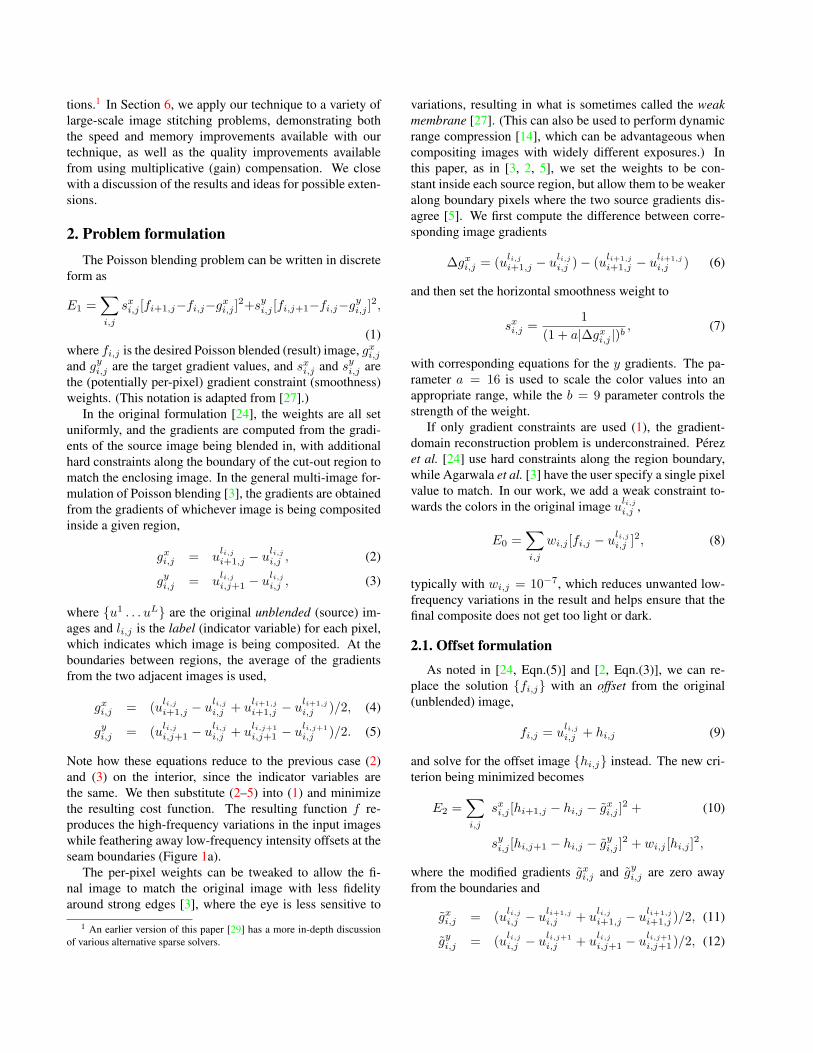
variations, resulting in what is sometimes called the weakmembrane [27]. (This can also be used to perform dynamicrange compression [14], which can be advantageous whencompositing images with widely different exposures.) Inthis paper, as in [3, 2, 5], we set the weights to be con-stant inside each source region, but allow them to be weakeralong boundary pixels where the two source gradients dis-agree [5]. We first compute the difference between corre-sponding image gradients

∆gxi,j = (uli,j

i+1,j − uli,j

i,j )− (uli+1,j

i+1,j − uli+1,j

i,j ) (6)

and then set the horizontal smoothness weight to

sxi,j =1

(1 + a|∆gxi,j |)b, (7)

with corresponding equations for the y gradients. The pa-rameter a = 16 is used to scale the color values into anappropriate range, while the b = 9 parameter controls thestrength of the weight.

If only gradient constraints are used (1), the gradient-domain reconstruction problem is underconstrained. Perezet al. [24] use hard constraints along the region boundary,while Agarwala et al. [3] have the user specify a single pixelvalue to match. In our work, we add a weak constraint to-wards the colors in the original image u

li,j

i,j ,

E0 =∑i,j

wi,j [fi,j − uli,j

i,j ]2, (8)

typically with wi,j = 10−7, which reduces unwanted low-frequency variations in the result and helps ensure that thefinal composite does not get too light or dark.

2.1. Offset formulation

As noted in [24, Eqn.(5)] and [2, Eqn.(3)], we can re-place the solution {fi,j} with an offset from the original(unblended) image,

fi,j = uli,j

i,j + hi,j (9)

and solve for the offset image {hi,j} instead. The new cri-terion being minimized becomes

E2 =∑i,j

sxi,j [hi+1,j − hi,j − gxi,j ]2 + (10)

syi,j [hi,j+1 − hi,j − gyi,j ]2 + wi,j [hi,j ]2,

where the modified gradients gxi,j and gyi,j are zero awayfrom the boundaries and

gxi,j = (uli,j

i,j − uli+1,j

i,j + uli,j

i+1,j − uli+1,j

i+1,j )/2, (11)

gyi,j = (uli,j

i,j − uli,j+1i,j + u

li,j

i,j+1 − uli,j+1i,j+1 )/2, (12)

i

i

(a) (b)

ui1

ui2

fihi

i

(c)hi1

hi2

ck2

ck1

Figure 1. One dimensional examples of Poisson blending and offset maps: (a) the original Poisson blend of two source images u1i and u2

i

produces the blended function fi; (b) the offset image hi is fitted to zero gradients everywhere except at the source image discontinuity,where it jumps by an amount equal to the average difference across the region boundary; (c) the multiple offset images h1

i and h2i , each of

which is smooth, along with the inter-image constraint at the boundary; the offsets are defined by the spline control vertices c1k and c2

k.

at the boundaries between regions.This new problem has a natural interpretation: the offset

value should be everywhere smooth, except at the regionboundaries, where it should jump by an amount equal tothe (negative) average difference in intensity between theoverlapping source images. The resulting offset function ispiecewise smooth (Figure 1b), which makes it amenable tobeing represented by a quadtree spline, with smaller gridcells closer to the region boundaries [2] or with mean valuecoordinate interpolation [12].

3. Multiple offset mapsIn this paper, instead of using a single offset map, as sug-

gested in [24, 2, 12], we use a different offset map for eachsource image, i.e.,

fi,j = uli,j

i,j + hli,j

i,j , (13)

where the {h1 . . . hl} are now the per-source image offsetmaps (see Figure 1c).

The optimization problem (10) now becomes

E3 =∑i,j

sxi,j [hli+1,j

i+1,j − hli,j

i,j − gxi,j ]2 + (14)

syi,j [hli,j+1i,j+1 − h

li,j

i,j − gyi,j ]2 + wi,j [h

li,j

i,j ]2,

Notice that in this problem, whenever two adjacent pixels,say (i, j) and (i + 1, j) come from the same source andhence share the same offset map, the gradient gxi,j is 0, andso the function is encouraged to be smooth. When two ad-jacent pixels come from different regions, the difference be-tween their offset values is constrained to be the averagedifference in source values at the two pixels (11). This isillustrated schematically in Figure 1c.

What is the advantage of re-formulating the problem us-ing a larger number of unknowns? There is none if we keepall of the hli,j as independent variables.

However, under normal circumstances, e.g., when work-ing with log intensities and multiplicative exposure differ-ences, each of the individual per-source offset maps will besmooth, and not just piecewise smooth as in the case of asingle offset map. Therefore, each offset map can be repre-sented at a much lower resolution, as we describe next.

4. Spline offset mapsTo take advantage of the smoothness of each offset im-

age, we represent each map with a tensor-product spline thatcovers the visible extent of each region, as shown in Fig-ure 2. The choice of pixel spacing (subsampling) S is prob-lem dependent, i.e., it depends on the amount of unmod-eled variations in the scene and acquisition process, e.g.,the severity of lens vignetting or the amount of inconsistenttexture along the seam, but is largely independent of theactual pixel (sensor) resolution. We can either align eachgrid with each region’s bounding box (Figure 2a) or use aglobally consistent alignment (Figure 2b). We use the latter,since it makes the nested dissection algorithm discussed inSection 5 easier to implement.

Once we have chosen S and the control grid locations,we can re-write each pixel in an individual offset map asa linear combination of the per-level spline control verticesclk,m (Figure 1c),

hli,j =∑km

clk,mB(i− kS, j −mS) (15)

whereB(i, j) = b(i)b(j) (16)

is a 2D tensor product spline basis and b(i) is a 1-D B-splinebasis function [13]. For example, when bilinear (first or-der) interpolation is used, as is the case in our experiments,the first order 1-D B-spline is the usual tent function, andeach pixel is a linear blend of its 4 adjacent control vertices(Figure 2c).

The values of hli,j in (15) can be substituted into (14)to obtain a new energy function (omitted for brevity) thatonly depends on the spline control variables clk,m. This newenergy function can be minimized as a sparse least squaressystem to compute a smooth spline-based approximation tothe offset fields. Once the sparse least squares system hasbeen solved, as described in Section 5, the per-pixel offsetvalues can be computed using regular spline interpolation(15).

The actual inner loop of the least squares system setupsimply involves iterating over all the pixels, pulling out the

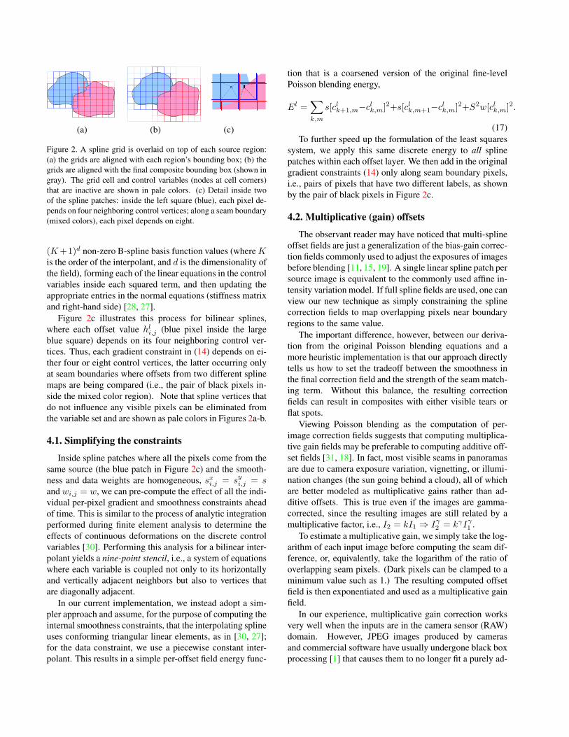
(a) (b) (c)

Figure 2. A spline grid is overlaid on top of each source region:(a) the grids are aligned with each region’s bounding box; (b) thegrids are aligned with the final composite bounding box (shown ingray). The grid cell and control variables (nodes at cell corners)that are inactive are shown in pale colors. (c) Detail inside twoof the spline patches: inside the left square (blue), each pixel de-pends on four neighboring control vertices; along a seam boundary(mixed colors), each pixel depends on eight.

(K +1)d non-zero B-spline basis function values (where Kis the order of the interpolant, and d is the dimensionality ofthe field), forming each of the linear equations in the controlvariables inside each squared term, and then updating theappropriate entries in the normal equations (stiffness matrixand right-hand side) [28, 27].

Figure 2c illustrates this process for bilinear splines,where each offset value hli,j (blue pixel inside the largeblue square) depends on its four neighboring control ver-tices. Thus, each gradient constraint in (14) depends on ei-ther four or eight control vertices, the latter occurring onlyat seam boundaries where offsets from two different splinemaps are being compared (i.e., the pair of black pixels in-side the mixed color region). Note that spline vertices thatdo not influence any visible pixels can be eliminated fromthe variable set and are shown as pale colors in Figures 2a-b.

4.1. Simplifying the constraints

Inside spline patches where all the pixels come from thesame source (the blue patch in Figure 2c) and the smooth-ness and data weights are homogeneous, sxi,j = syi,j = sand wi,j = w, we can pre-compute the effect of all the indi-vidual per-pixel gradient and smoothness constraints aheadof time. This is similar to the process of analytic integrationperformed during finite element analysis to determine theeffects of continuous deformations on the discrete controlvariables [30]. Performing this analysis for a bilinear inter-polant yields a nine-point stencil, i.e., a system of equationswhere each variable is coupled not only to its horizontallyand vertically adjacent neighbors but also to vertices thatare diagonally adjacent.

In our current implementation, we instead adopt a sim-pler approach and assume, for the purpose of computing theinternal smoothness constraints, that the interpolating splineuses conforming triangular linear elements, as in [30, 27];for the data constraint, we use a piecewise constant inter-polant. This results in a simple per-offset field energy func-

tion that is a coarsened version of the original fine-levelPoisson blending energy,

El =∑k,m

s[clk+1,m−clk,m]2+s[clk,m+1−clk,m]2+S2w[clk,m]2.

(17)To further speed up the formulation of the least squares

system, we apply this same discrete energy to all splinepatches within each offset layer. We then add in the originalgradient constraints (14) only along seam boundary pixels,i.e., pairs of pixels that have two different labels, as shownby the pair of black pixels in Figure 2c.

4.2. Multiplicative (gain) offsets

The observant reader may have noticed that multi-splineoffset fields are just a generalization of the bias-gain correc-tion fields commonly used to adjust the exposures of imagesbefore blending [11, 15, 19]. A single linear spline patch persource image is equivalent to the commonly used affine in-tensity variation model. If full spline fields are used, one canview our new technique as simply constraining the splinecorrection fields to map overlapping pixels near boundaryregions to the same value.

The important difference, however, between our deriva-tion from the original Poisson blending equations and amore heuristic implementation is that our approach directlytells us how to set the tradeoff between the smoothness inthe final correction field and the strength of the seam match-ing term. Without this balance, the resulting correctionfields can result in composites with either visible tears orflat spots.

Viewing Poisson blending as the computation of per-image correction fields suggests that computing multiplica-tive gain fields may be preferable to computing additive off-set fields [31, 18]. In fact, most visible seams in panoramasare due to camera exposure variation, vignetting, or illumi-nation changes (the sun going behind a cloud), all of whichare better modeled as multiplicative gains rather than ad-ditive offsets. This is true even if the images are gamma-corrected, since the resulting images are still related by amultiplicative factor, i.e., I2 = kI1 ⇒ Iγ2 = kγIγ1 .

To estimate a multiplicative gain, we simply take the log-arithm of each input image before computing the seam dif-ference, or, equivalently, take the logarithm of the ratio ofoverlapping seam pixels. (Dark pixels can be clamped to aminimum value such as 1.) The resulting computed offsetfield is then exponentiated and used as a multiplicative gainfield.

In our experience, multiplicative gain correction worksvery well when the inputs are in the camera sensor (RAW)domain. However, JPEG images produced by camerasand commercial software have usually undergone black boxprocessing [1] that causes them to no longer fit a purely ad-

(a) (b)

(c) (d)

Figure 3. Comparison of multiplicative gain vs. additive offsetblending: (a) unblended image; (b) additive offset blending; (c)square root offset blending; (d) multiplicative gain blending. Notehow the additive result has a visible contrast change across theseam.

ditive or multiplicative model. For this reason we prefer tocompute the offset field in a log/linear domain. In our expe-rience, the square root function approximates the log func-tion well for bright values and approaches linear for darkvalues. In our implementation, we apply the square rootfunction (with pixels normalized to a [0, 1] range) to eachpixel before computing the seam differences. The resultingoffset field is then added to the square root pixel values andthe result is then squared.

Figure 3 compares the result using the multiplicativegain approach vs. the traditional additive Poisson blend-ing approach. Because the additive offset does not modelthe differing amounts of contrast in the two source images(which are related by a multiplicative exposure difference),the blended result in Figure 3b has a visible contrast changein the vicinity of the seam (more muddy looking colors tothe right of the seam, which are better seen in the supple-mentary materials).

4.3. Laplacian pyramid blending

While Poisson blending does a good job of compensat-ing for slowly varying differences between images such asexposure or lighting changes, it has a harder time hiding ar-tifacts due to inhomogeneous (inconsistent) textures in thetwo images. Consider, for example, the wave-tossed watersshown in Figure 4. While Poisson blending does a good jobof disguising low-frequency color and intensity differences,the differences between the individual wave patterns resultin visible seams. Applying multi-band Laplacian pyramidblending [9, 7] with a small number of pyramid levels to

(a) (b)

Figure 4. Using Laplacian pyramid blending to disguise texturedifferences: (a) image robustly blended in the square root pixeldomain; (b) with the addition of three-level Laplacian pyramidblending. Note how the differences in the wave patterns and smallmisalignments are effectively masked.

the gain or bias-compensated images helps disguise thesedifferences. Since our multi-spline Poisson blending effec-tively handles the low frequency differences between theimages, there is no need to use a large number of pyra-mid levels. The multi-level pyramid filtering operations cantherefore be restricted to a narrow band around the seams,which can lead to large computational savings.

4.4. Blending Gigapixel images

To make our technique even more efficient, instead ofcomputing the seam costs at the final image resolution, wecompute these costs at the same resolution as the graph cutoptimization performed in [20], which is 1/8th the horizon-tal and vertical resolution of the final panorama.

The decision to accumulate the seam costs on a lowerresolution image is actually well-justified. Since the rela-tive contribution of each seam constraint to the spline ver-tices is a slowly varying function, summing these contribu-tions over a slightly coarser grid than the pixels (but stillfiner than the spline) does not affect the results very much.Because we are computing a least squares correction, sum-ming up the least squares contributions over regions doesnot affect the final cost, except for the replacement of thespline weights with a slightly more discretized version.

Another way of looking at this is that if we are estimatingthe offset or gain adjustment between overlapping images, asimilar result will be obtained if we look at lower-resolutionversions of these images, so long as the lowered resolutionis still significantly higher than the spline grid.

Once we have computed our multi-spline correctionfields [29], these are then upsampled to the final Gigapixelresolution during the tile-based final compositing process[20].

5. Solving the systemA variety of techniques can be used to solve the small

sparse positive definite system of equations arising from themulti-spline correction fields. For large sparse system, it-erative techniques (potentially enhanced with multi-grid ormulti-level preconditioning) can be used [25]. When thesystems are smaller, direct factorization techniques such asCholesky decomposition are more efficient [10].

Because his sparse systems are larger, Agarwala [2] usesthe conjugate gradient sparse iterative solver, which par-tially accounts for his longer run times. Because our multi-spline systems are much smaller, we use direct techniques.The efficiency of these techniques depends on the amountof fill-in during the factorization process, which can be re-duced by an appropriate reordering of the variables [10, 29].

For two-dimensional grid problems, nested dissec-tion, which recursively splits the problem along smalllength rows or columns, results in good performance, i.e.,O(n log n) space and O(n3/2) time (or better for asymmet-rically shaped domains), where n is the number of vari-ables. In order for this technique to work, we need to en-sure that all the spline variables line up in the same rowsand columns, which is why we use the aligned spline gridshown in Figure 2b.

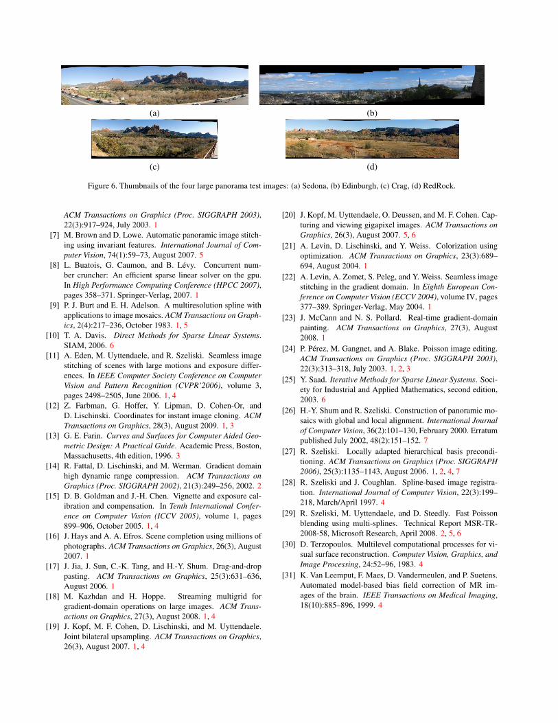
6. ExperimentsIn order to validate our approach and to see how much

of a speedup could be expected, we first obtained the fourlarge panoramas shown in Figure 6 from the author of [2].For these images, we used an additive offset field to matchthe results presented in [2] as closely as possible. We alsoused a spline spacing of S = 64 and bilinear splines.

The results of running our algorithm (in January, 2008)[29] on these four data sets are shown in Table 2. Our multi-spline technique is about 5–10× faster and requires about10× less memory than the quadtree-based approach devel-oped in [2]. The two techniques produce results of compa-rable visual quality, as can be seen by inspecting the largefull-size images provided in the supplementary material.

Grid size S RMS error max error solve time (s)8 0.0886 11.20 163.383

16 0.1039 12.80 11.71432 0.1841 13.70 0.85164 0.2990 14.40 0.070

128 0.4118 13.90 0.019

Table 1. RMS and maximum error comparisons to the groundtruth Poisson blend for different grid sizes S, along with the linearsystem solution time (in seconds); the time for setup and renderingthe final offset fields is about 2 seconds. For these experiments, weused the 9.7 Mpixel St. Emilion dataset shown in Figure 5.

Table 1 shows how the RMS (root mean square) andmaximum error (in gray levels) in the solution depend onthe grid size S. For these experiments, we used the so-lution to the St. Emilion data set provided by Agarwala[2] (Figure 5) as our ground truth. We then ran our fastmulti-spline-based solver using a variety of grid sizes, S ={8, 16, . . . , 128} and computed both the RMS and maxi-mum error between the offset field we computed and thefull solution. As you can see, the RMS error grows steadilywith the grid size, while the maximum error does not varythat much. Visual inspection of the full-resolution results(which are available as part of the supplementary materials)shows that the maximum error is concentrated at isolatedpixels along seam boundaries where highly textured regionsare mis-aligned. Fortunately, these “errors” are masked bythe textures themselves, so that the final blended images ap-pear of identical quality to the eye.

Next, we applied our technique to the Seattle Skyline im-age shown in Figure 4 of [20], using the multiplicative gain(log intensity) formulation because of the large exposuredifferences. In this case, because the seam costs were com-puted on a 1/8th (on side) resolution image, the seam costevaluation (shown as Setup in Table 2) and system solvingtimes as well as the memory requirement are comparable tothose of the 84 Mpixel RedRock panorama. The renderingtime required to read back and warp the source images, ap-ply the spline-based correction, and write out the resultingtiles is significantly longer.

A cropped portion of our result is shown in Figure 5,and the unblended, offset, and blended images at the 1/8thworking resolution, along with some cropped portions ofthe final Gigapixel image are shown in the supplementarymaterials.

The most visible artifacts in these results, besides the sat-urated regions and gross misalignments caused by the mov-ing crane, are the occasional seams visible in the sky regionsnear dark buildings, which are due to some of the originalsource images having saturated pixels (usually in the bluechannel) in these regions. Unfortunately, since the values atthese pixels do not reflect the true irradiance, the multiplica-tive gain computed in areas that border unsaturated pixels isinconsistent, and cannot simultaneously hide both kinds ofseams.

7. Discussion and extensionsAs we can see from our experiments, the biggest dif-

ference between our multi-spline approach and full Pois-son blending (and its quadtree approximation) is that weenforce piecewise smoothness in both the x and y dimen-sions, whereas Poisson blending can tolerate irregular off-sets along the seam. While our approach can occasion-ally lead to artifacts, e.g., in images that are not log-linear,Poisson blending can introduce different artifacts, such as

(a) (b) (c)

Figure 5. Fast Poisson blending using multi-splines: (a) unblended composite; (b) piecewise smooth multi-spline offset image; (c) finalblended composite.

Quadtree Multi-spline Setup Solve RenderDataset # Mpix V (%) T (s) M V (%) T (s) M T (s) M T (s) M T (s)Sedona 6 34.6 0.47 29 52 0.0271 7 4 3.33 3 0.28 5 2.70Edinburgh 25 39.7 1.15 122 123 0.0315 9 10 3.99 10 0.41 7 3.84Crag 7 62.7 0.47 78 96 0.0271 12 7 6.16 6 0.54 9 4.82RedRock 9 83.7 0.46 118 112 0.0270 16 10 8.11 8 0.75 13 6.42Seattle 650 3186.9 0.0009 8+ 57 6.35 57 1.42 34 56m

Table 2. Performance of the quadtree vs. multi-spline based solver. The first three columns list the dataset name, the number of sourceimages, and the number of pixels. The next three columns show the results for the quadtree-based acceleration, including the ratio ofvariables to original pixels (as a percentage), the total run time (in seconds), and the memory usage (in Mbytes). The next three columnsshow the corresponding results for our multi-spline based approach (for all of our experiments, S = 64). Our results are roughly 5–10× faster and smaller. The final sets of columns break down the time and memory requirements of the three multi-spline blendingstages, namely the setup (computation of seam boundary constraints), the direct solution using nested dissection, and the final rendering(compensation) stage. The numbers in the Quadtree column are from [2], which does not report the processor used. The numbers in theother columns are from experiments run single-threaded on a 2.40 Intel GHz CoreTM2 Duo processor with 4GB RAM purchased in March,2007, and therefore likely comparable to the processor used by Agarwala. Note that the Gigapixel Seattle total time (8+) does not includethe i/o bound rendering stage, which took 56 minutes to produce the final image tile set.

“ruffles” that sometime propagate away from seam bound-aries when they disagree. Improving the alignment betweenimages using an optic-flow deghosting technique [26] fol-lowed by robustly estimating the mapping between over-lapping images is likely to futher improve the results.

In terms of computational complexity, as the resolutionof photographs continues to increase, our multi-spline basedapproach has better scaling properties that the quadtreebased approach. Because the number of spline control ver-tices depends on the smoothness of the unmodeled inter-exposure variation and not the pixel density, we expect it toremain fixed. In the quadtree-based approach, the numberof variables increases linearly with the on-side (as opposedto pixel count) resolution. In order to further speed up thelinear system solving part of our algorithms, we are alsoinvestigating hierarchically preconditioned conjugate gradi-ent descent [27].

8. ConclusionsIn this paper, we have developed a new approach

to gradient domain compositing that allocates a separatesmoothly varying spline correction field for each source im-age. We also investigated the benefits of using a multiplica-tive gain formulation over the more traditional additive off-set formulation. Using our approach, we obtain linear sys-tems an order of magnitude smaller than those obtained with

a quadtree representation of a single offset map, while pro-ducing results of comparable visual quality. We also sug-gest areas for further investigations into better quality algo-rithms for seam blending.

References[1] Adobe. Digital Negative (DNG) Specification. Version

1.3.0.0, June 2009. 4[2] A. Agarwala. Efficient gradient-domain compositing using

quadtrees. ACM Transactions on Graphics, 26(3), August2007. 1, 2, 3, 6, 7

[3] A. Agarwala, M. Dontcheva, M. Agrawala, S. Drucker,A. Colburn, B. Curless, D. H. Salesin, and M. F. Cohen.Interactive digital photomontage. ACM Transactions onGraphics (Proc. SIGGRAPH 2004), 23(3):292–300, August2004. 1, 2

[4] P. Bhat, B. Curless, M. Cohen, and C. L. Zitnick. Fourieranalysis of the 2D screened Poisson equation for gradientdomain problems. In Tenth European Conference on Com-puter Vision (ECCV 2008), pages 114–128. Springer-Verlag,October 2008. 1

[5] P. Bhat, C. L. Zitnick, M. F. Cohen, and B. Curless. Gra-dientshop: A gradient-domain optimization framework forimage and video filtering. ACM Transactions on Graphics,29(2), March 2010. 2

[6] J. Bolz, I. Farmer, E. Grinspun, and P. Schroder. Sparse ma-trix solvers on the GPU: Conjugate gradients and multigrid.

(a) (b)

(c) (d)

Figure 6. Thumbnails of the four large panorama test images: (a) Sedona, (b) Edinburgh, (c) Crag, (d) RedRock.

ACM Transactions on Graphics (Proc. SIGGRAPH 2003),22(3):917–924, July 2003. 1

[7] M. Brown and D. Lowe. Automatic panoramic image stitch-ing using invariant features. International Journal of Com-puter Vision, 74(1):59–73, August 2007. 5

[8] L. Buatois, G. Caumon, and B. Levy. Concurrent num-ber cruncher: An efficient sparse linear solver on the gpu.In High Performance Computing Conference (HPCC 2007),pages 358–371. Springer-Verlag, 2007. 1

[9] P. J. Burt and E. H. Adelson. A multiresolution spline withapplications to image mosaics. ACM Transactions on Graph-ics, 2(4):217–236, October 1983. 1, 5

[10] T. A. Davis. Direct Methods for Sparse Linear Systems.SIAM, 2006. 6

[11] A. Eden, M. Uyttendaele, and R. Szeliski. Seamless imagestitching of scenes with large motions and exposure differ-ences. In IEEE Computer Society Conference on ComputerVision and Pattern Recognition (CVPR’2006), volume 3,pages 2498–2505, June 2006. 1, 4

[12] Z. Farbman, G. Hoffer, Y. Lipman, D. Cohen-Or, andD. Lischinski. Coordinates for instant image cloning. ACMTransactions on Graphics, 28(3), August 2009. 1, 3

[13] G. E. Farin. Curves and Surfaces for Computer Aided Geo-metric Design: A Practical Guide. Academic Press, Boston,Massachusetts, 4th edition, 1996. 3

[14] R. Fattal, D. Lischinski, and M. Werman. Gradient domainhigh dynamic range compression. ACM Transactions onGraphics (Proc. SIGGRAPH 2002), 21(3):249–256, 2002. 2

[15] D. B. Goldman and J.-H. Chen. Vignette and exposure cal-ibration and compensation. In Tenth International Confer-ence on Computer Vision (ICCV 2005), volume 1, pages899–906, October 2005. 1, 4

[16] J. Hays and A. A. Efros. Scene completion using millions ofphotographs. ACM Transactions on Graphics, 26(3), August2007. 1

[17] J. Jia, J. Sun, C.-K. Tang, and H.-Y. Shum. Drag-and-droppasting. ACM Transactions on Graphics, 25(3):631–636,August 2006. 1

[18] M. Kazhdan and H. Hoppe. Streaming multigrid forgradient-domain operations on large images. ACM Trans-actions on Graphics, 27(3), August 2008. 1, 4

[19] J. Kopf, M. F. Cohen, D. Lischinski, and M. Uyttendaele.Joint bilateral upsampling. ACM Transactions on Graphics,26(3), August 2007. 1, 4

[20] J. Kopf, M. Uyttendaele, O. Deussen, and M. F. Cohen. Cap-turing and viewing gigapixel images. ACM Transactions onGraphics, 26(3), August 2007. 5, 6

[21] A. Levin, D. Lischinski, and Y. Weiss. Colorization usingoptimization. ACM Transactions on Graphics, 23(3):689–694, August 2004. 1

[22] A. Levin, A. Zomet, S. Peleg, and Y. Weiss. Seamless imagestitching in the gradient domain. In Eighth European Con-ference on Computer Vision (ECCV 2004), volume IV, pages377–389. Springer-Verlag, May 2004. 1

[23] J. McCann and N. S. Pollard. Real-time gradient-domainpainting. ACM Transactions on Graphics, 27(3), August2008. 1

[24] P. Perez, M. Gangnet, and A. Blake. Poisson image editing.ACM Transactions on Graphics (Proc. SIGGRAPH 2003),22(3):313–318, July 2003. 1, 2, 3

[25] Y. Saad. Iterative Methods for Sparse Linear Systems. Soci-ety for Industrial and Applied Mathematics, second edition,2003. 6

[26] H.-Y. Shum and R. Szeliski. Construction of panoramic mo-saics with global and local alignment. International Journalof Computer Vision, 36(2):101–130, February 2000. Erratumpublished July 2002, 48(2):151–152. 7

[27] R. Szeliski. Locally adapted hierarchical basis precondi-tioning. ACM Transactions on Graphics (Proc. SIGGRAPH2006), 25(3):1135–1143, August 2006. 1, 2, 4, 7

[28] R. Szeliski and J. Coughlan. Spline-based image registra-tion. International Journal of Computer Vision, 22(3):199–218, March/April 1997. 4

[29] R. Szeliski, M. Uyttendaele, and D. Steedly. Fast Poissonblending using multi-splines. Technical Report MSR-TR-2008-58, Microsoft Research, April 2008. 2, 5, 6

[30] D. Terzopoulos. Multilevel computational processes for vi-sual surface reconstruction. Computer Vision, Graphics, andImage Processing, 24:52–96, 1983. 4

[31] K. Van Leemput, F. Maes, D. Vandermeulen, and P. Suetens.Automated model-based bias field correction of MR im-ages of the brain. IEEE Transactions on Medical Imaging,18(10):885–896, 1999. 4