fast optimal joint tracking–registration for multisensor systems

IEEE TRANSACTIONS ON INSTRUMENTATION AND MEASUREMENT, VOL. 60, NO. 10, OCTOBER 2011 3461

Fast Optimal Joint Tracking–Registrationfor Multisensor Systems

Shuqing Zeng, Member, IEEE

Abstract—Sensor fusion of multiple sources plays an importantrole in vehicular systems to achieve refined target position and ve-locity estimates. In this paper, we address the general registrationproblem, which is a key module for a fusion system to accuratelycorrect systematic errors of sensors. A fast maximum a posteriori(FMAP) algorithm for joint registration–tracking is presented.The algorithm uses a recursive two-step optimization that involvesorthogonal factorization to ensure numerically stability. Statisticalefficiency analysis based on Cramèr–Rao lower bound theory ispresented to show asymptotical optimality of FMAP. In addition,Givens rotation is used to derive a fast implementation withcomplexity O(n), with n being the number of tracked targets.Simulations and experiments are presented to demonstrate thepromise and effectiveness of FMAP.

Index Terms—Bayesian network, Cramèr–Rao lower bound,Givens rotation, least-squares estimation, sensor registration,target tracking.

I. INTRODUCTION

R ECENTLY, active safety driver assistance (ASDA) sys-tems such as adaptive cruise control and precrash sensing

systems [5] have drawn considerable attention in intelligenttransportation systems community. To obtain the necessaryinformation of surround vehicles for ASDA systems, multiplesensors, including active radars, lidars, and passive cameras,are mounted on vehicles. Those sensor systems in a vehicularsystem are typically calibrated manually. However, sensor ori-entation and signal output may drift during the life of the sensor,such that the orientation of the sensor relative to the vehicularframe is changed. When the sensor orientation drifts, measure-ments become skewed relative to the vehicle [14]. When thereare multiple sensors, this concern is further complicated. It isthus desirable to have sensor systems that automatically alignsensor output to the vehicular frame [1], [2].

Two categories of approaches have attempted to address theregistration problem. The first category decouples tracking andregistration into separate problems. In [7], [10], [12], and [20],filters are designed to estimate the sensor biases by minimizingthe discrepancy between measurements and associated fusedtarget estimates from a separated tracking module. However,these methods are not optimal in terms of Cramèr–Rao bounds

Manuscript received September 21, 2010; revised December 17, 2010;accepted February 2, 2011. Date of publication May 5, 2011; date of currentversion September 14, 2011. The Associate Editor coordinating the reviewprocess for this paper was Dr. Antonios Tsourdos.

The author is with the Research and Development Center, General MotorsCorporation, Warren, MI 48090 USA.

Color versions of one or more of the figures in this paper are available onlineat http://ieeexplore.ieee.org.

Digital Object Identifier 10.1109/TIM.2011.2134990

[18]. In the second category, the approaches jointly solve fortarget tracking and sensor registration. For example, the studiesin [15], [16], and [19] have applied extended Kalman filtering(EKF) to an augmented state vector, combining the targetvariables and sensor system errors in aerospace applications. In[6], a fixed-lag smoothing framework is employed to estimatethe augmented state vector to deal with communication jitters innetworked sensors. Unscented Kalman filter (UKF) in [11] andexpectation–maximization-based interacting multiple model in[9] have been applied to the augmented state vector in vehicle-to-vehicle cooperative driving systems. In [17], the particlefilter outperforms EKF at the cost of more demanding com-putations in state estimation for industrial systems. However,there are a few difficulties with these approaches. Since theregistration parameters are constant, the error model of statespace is degenerated. This not only makes the estimation prob-lem larger—leading to higher computational cost (complexityO(n3), with n denoting the number of targets), but also resultsdegenerated covariance matrices for the process noise vectorsdue to numerical instability inherent to EKF, UKF, and thevariants.

In this paper, we propose a fast maximum a posteriori(FMAP) registration algorithm to tackle the problems. We com-bine all the measurement equations and process equations toform a linearized state-space model. The registration and targettrack estimates are obtained by maximizing a posterior functionin the state space. The performance of FMAP estimates isexamined using Cramèr-Rao lower bound (CRLB) theory. Byexploiting the sparsity of the Cholesky factor of informationmatrix, a fast implementation whose complexity scales linearlywith the numbers of targets and measurements is derived.

The rest of this paper is organized as follows. Section II is de-voted to the algorithm derivation. The results of simulation andexperiment are presented in Sections III and IV, respectively.Finally, we give concluding remarks in Section V.

II. ALGORITHM DERIVATION

In this section, we address the computational issues in usingan EKF or UKF to solve joint tracking–registration (JTR).Fig. 1 shows the results of a joint problem with ten tracks andsix registration parameters. The normalized covariance of thejoint state from EKF is visualized in Fig. 1(a). Dark entriesindicate strong correlations. It is clear that not only the tracksx and the registration a are correlated but also each pair oftracks in x is mutually correlated. The checkerboard appearanceof the joint covariance matrix reveals this fact. Therefore, the

0018-9456/$26.00 © 2011 IEEE

3462 IEEE TRANSACTIONS ON INSTRUMENTATION AND MEASUREMENT, VOL. 60, NO. 10, OCTOBER 2011

Fig. 1. Typical snapshot of correlation matrices for JTR with ten tracks x andsix registration parameters a. (a) Correlation matrix P of EKF (normalized).(b) Normalized Cholesky factor R of inverse covariance.

approximation that ignores the off-diagonal correlated entries[20] is not asymptotical optimal.

A key insight that motivates the proposed approach is shownin Fig. 1(b). Shown there is the Cholesky factor1 of the inversecovariance matrix (also known as information matrix) normal-ized like the correlation matrix. Entries in this matrix can beregarded as constraints, or connections, between the locationsof targets and registration parameters. The darker an entry is inthe display, the stronger the connection is. As this illustrationsuggests, the Cholesky factor R not only appears sparse butalso is nicely structured. The matrix is only dominated bythe entries within a track, or the entries between a track andthe registration parameters. The proposed FMAP algorithmexploits and maintains this structure throughout the calculation.In addition, storing a sparse factor matrix requires linear space.More importantly, updates can be performed in linear time withregard to the number of tracks in the system.

The sparsity of information matrix has been widely used toderive fast implementations of robotic simultaneous localiza-tion and mapping (SLAM) [3], [13]. In those approaches, theauthors insightfully observed that the resulting information ma-trix is sparse if the measurements involve only “local” variables.However, the sparsity is destroyed in time-propagation stepswhere old robotic poses are removed from the state represen-tation by marginalization. Approximations (e.g., [8] and [13])are needed to enforce sparsity during the marginalization.

Although inspired by SLAM information filters, FMAP isdifferent in the following aspects.

1) JTR and SLAM are different problems despite the sim-ilarity between their system dynamics equations. Thenumber of stationary landmarks dominates the time com-plexity in the SLAM case. On the other hand, the numberof tracked targets that are in stochastic motion determinesthe time complexity in the JTR case.

2) Unlike SLAM, FMAP needs no approximation to enforcethe sparsity in the measurement update and time propaga-tion, as shown in Fig. 1(b).

3) FMAP recursively computes the Cholesky factor of infor-

mation matrix R =[

Rx Rxa

0 Ra

]as shown in Fig. 1(b),

1The Cholesky factor R of a matrix P is defined as P = RtR. A semiposi-tive definite matrix can be decomposed into its Cholesky factor.

contrasting the fact that information matrix is computedin the SLAM case. In addition, marginalization of oldtracked targets x′ does not destroy the sparsity of R.

Throughout this paper, italic upper and lower case letters areused to denote matrices and vectors, respectively. A Gaussiandistribution is denoted by information array [4]. For example,a multivariate x with density function N(x, Q) is denoted asp(x) ∝ e(−(‖Rx−z‖2/2)) or the information array [R, z] in short,where z = Rx and Q = R−1R−T .

A. Joint State Space

The setting for the JTR problem is that a vehicle, equippedwith multiple sensors with unknown or partially unknown regis-tration, moves through an environment containing a populationof objects. The sensors can take measurements of the relativeposition and velocity between any individual object and thevehicle.

The objective here is to derive a joint dynamics model wheren tracks and registration parameters from k sensors are stackedinto one large state vector, such as follows:

s = [xT1 xT

2 · · · xTn aT

1 · · · aTk ]T

where the ith target track xi (i = 1, . . . , n) comprises a set ofparameters, e.g., position, velocity, and acceleration, and theregistration parameters for the jth sensor aj (j = 1, . . . , k) arecomposed of a location error, an azimuth alignment error, andrange offset.

The system dynamics equation for the state is expressed as

s(t + 1) = f (s(t), w(t)) (1)

where the function relates the state at time t to the state attime t + 1 and where terms w’s are vectors of zero-meannoise random variables that are assumed to have nonsingularcovariance matrices.

The measurement process can be modeled symbolically asa function of target track (x), and registration parameter (a),such as

o(t) = h (x(t), a(t)) + v(t) (2)

where o(t) and v(t) denote the measurements and the additivenoise vectors at time instant t, respectively.

B. Measurement Update

The FMAP algorithm works with the posterior density func-tion p(s(t) | o(0:t)), where o(0:t) denotes a series of measure-ments {o(0), . . . , o(t)} from the sensors.

Using the Bayes rule, we obtain the posterior function as

p(s(t) | o(0:t)

)=p

(s(t) | o(0:t−1), o(t)

)=c1(t)p

(o(t) | o(0:t−1), s(t)

)p(s(t) | o(0:t−1)

)(3)

with c1(t) denoting the normalization factor. Typically, we willassume that measurements at time t depend only on the current

ZENG: FAST OPTIMAL JOINT TRACKING–REGISTRATION FOR MULTISENSOR SYSTEMS 3463

state s(t),2 and (3) can be written as

p(s(t) | o(0:t)

)= c1(t)p (o(t) | s(t)) p

(s(t) | o(0:t−1)

). (4)

Assuming that the density functions are normally distributed,the prior density function3 p(s | o(0:t−1)) can be expressed byinformation array [R, z], i.e.,

p(s | o(0:t−1)

)=

|R|(2π)Ns/2

exp

(−‖Rs − z‖2

2

)

=|R|

(2π)Ns/2

×exp

⎛⎜⎜⎜⎝−

∥∥∥∥[

Rx Rxa

0 Ra

] [xa

]−[

zx

za

]∥∥∥∥2

2

⎞⎟⎟⎟⎠(5)

where |R| is the determinant of R and Ns is the dimensionof s.

Linearizing (2) using Taylor expansion in the neighborhood[x∗, a∗] produces

o = Cxx + Caa + u1 + v (6)

with u1 = h∗ − Cxx∗ − Caa∗, h∗ = h(x∗, a∗), and Jacobianmatrices Cx and Ca. Without loss of generality, the covariancematrix of v is assumed to be an identity matrix.4 Thus, themeasurement density function can be written as

p(o | s)=1

(2π)No/2·exp

⎛⎜⎜⎜⎝−

∥∥∥∥[ Cx Ca ][

xa

]−(o−u1)

∥∥∥∥2

2

⎞⎟⎟⎟⎠(7)

with No being the dimension of o.The negative logarithm of (4) is given by

Jt = − log p(s | o(0:t)

)= − log p(o | s) − log p

(s | o(0:t−1)

)− log(c1). (8)

Plugging in (5) and (7), (8) becomes

Jt =

∥∥∥∥∥∥⎡⎣ Rx Rxa

0 Ra

Cx Ca

⎤⎦[x

a

]−

⎡⎣ zx

za

o − u1

⎤⎦∥∥∥∥∥∥

2

2+ c2 (9)

with c2 denoting terms not depending on (x, a).

2In Bayesian filtering, the state variables are designed such that they containall information gathered from the past measurements. Thus, s(t) is a sufficientstatistics of the past measurements o(0:t−1).

3Unless it is necessary, we will not include time such as (t) in all thefollowing equations.

4If not, the noise term v in (6) can be transformed to a random vector withidentity covariance matrix. Let cov{v} = Rv denote the covariance matrix ofthe measurement model. Multiplying both sides of (6) by Lv , the square rootinformation matrix of Rv results in a measurement equation with an identitycovariance matrix.

The principle of the maximum a posteriori estimation is tomaximize the posterior function with respect to the unknownvariables (x, a). Clearly, the maximization process is equiva-lent to minimization of the squared norm in (9). Ignoring theconstant term, the right-hand side (RHS) of (9) can be writtenas a matrix X expressed as

X =

⎡⎣ Rx Rxa zx

0 Ra za

Cx Ca o − u1

⎤⎦ (10)

where X can be turned into an upper triangular matrix byapplying an orthogonal transformation T

TX =

⎡⎣ Rx Rxa zx

0 Ra za

0 0 e

⎤⎦ (11)

with e being the residual that reflects the discrepancy betweenthe model and measurement. Applying orthogonal T to thequadratic term in (9) produces5

Jt =

∥∥∥∥[

Rx Rxa

0 Ra

] [xa

]−[

zx

za

]∥∥∥∥2

2+ c3 (12)

with c3 = c2 + (1/2)‖e‖2 denoting the constant term withrespect to variables (x, a).

Because Jt is the negative logarithm of p(s | o(0:t)), theposterior density can be written as

p(s | o(0:t)

)∝ e−

∥∥∥∥[Rx Rxa

0 Ra

][xa

]−

[zx

za

]∥∥∥∥2

2 (13)

or in the information-array form

[R, z] =[

Rx Rxa zx

0 Ra za

]. (14)

Since the estimate of the state variable s can be written ass = R−1z, (14) allows us to solve the estimates of the trackvariables x and registration parameters a by back substitutionusing R and RHS z, i.e.,[

Rx Rxa

0 Ra

] [xa

]=[

zx

za

]. (15)

C. Time Propagation

The prior density p(s(t + 1) | o(0:t)) at time t + 1 canbe inferred from the system dynamics and posterior functionp(s | o(0:t)) at time t. Assuming that registration is timeinvariant, the linear approximation of the system dynamics in(1) in the neighborhood [s∗, w∗] can be expressed as[

x(t + 1)a(t + 1)

]=[

Φx 00 I

] [xa

]+[

Gx

0

]w +

[u2

0

](16)

5The least squares ‖Rs − z‖2 is invariant under an orthogonal transforma-tion T , i.e., ‖T (Rs − z)‖2 = (Rs − z)tT tT (Rs − z) = (Rs − z)t(Rs −z) = ‖Rs − z‖2.


where Φx and Gx are Jacobian matrices and the nonlinear termu2 = f(s∗, w∗) − Φxx∗ − Gxw∗.

If variables s and w are denoted by the information arrays in(14) and [Rw, zw], respectively, the joint density function giventhe measurements o(0:t) can be expressed in terms of x(t + 1)and a(t + 1) as6

p(s(t + 1), w | o(0:t)

)∝ e−

‖Asw−b‖2

2 (17)

with A =

⎡⎣ Rw 0 0−RxΦ−1

x Gx RxΦ−1x Rxa

0 0 Ra

⎤⎦, sw =

⎡⎣ w

x(t + 1)a(t + 1)

⎤⎦, and b =

⎡⎣ zw

zx + RxΦ−1x u2

za

⎤⎦.

The quadratic exponential term in (17) can be denoted asmatrix Y , expressed as

Y = [A b]. (18)

The matrix Y can be turned into a triangular matrix through anorthogonal transformation T , i.e.,

T Y = [A b] (19)

with A =

⎡⎣ Rw(t + 1) Rwx(t + 1) Rwa(t + 1)

0 Rx(t + 1) Rxa(t + 1)0 0 Ra(t + 1)

⎤⎦ and

b =

⎡⎣ zw(t + 1)

zx(t + 1)za(t + 1)

⎤⎦.

Given the measurements o(0:t), the prior function p(s(t +1) | o(0:t)) can be produced by marginalization on variable w.Applying Lemma 6.3 in the Appendix, we obtain the equationshown at the bottom of the page, with c4 being the normaliza-tion factor.

Therefore, we obtain the updated prior information array[R(t + 1), z(t + 1)] at time t + 1 as[

Rx(t + 1) Rxa(t + 1) zx(t + 1)0 Ra(t + 1) za(t + 1)

]. (20)

The derivation leading to (20) illustrates the purposes of usingthe information array [R, z], which is recursively updated to[R(t + 1), z(t + 1)] at time instant t + 1.

D. Algorithm

Fig. 2 shows the flowchart of FMAP. The algorithm isstarted upon reception of sensor data, and the state variablesof every track and registration parameters are initialized usingzero-mean noninformative distributions, respectively. A data

6Detailed derivation is shown in Lemma 6.2 in the Appendix.

Fig. 2. Flowchart of the FMAP algorithm.

association module matches the sensor data with the predictedlocation of targets. The measurement update module combinesthe previous estimation (i.e., prior) and new data (i.e., matchedmeasurement–track pairs) and updates target estimation andregistration. FMAP checks whether the discrepancy betweenmeasurements and predictions (innovation error) is larger thana threshold T . A change of registration parameters is detectedwhen the threshold is surpassed, and the prior of the sensorregistration is reset to the noninformative distribution. This typ-ically occurs when the sensor’s pose is significantly moved. Thetime propagation module predicts the target and registration inthe next time instant based on the dynamics model (16).

The complete specification of the proposed algorithm isgiven in Algorithm 1. Note that the prior [R0, z0] at time 0 isinitialized as R0 = εI and z0 = 0, where ε is a small positivenumber and I is an identity matrix of appropriate dimension.

Although static registration a is assumed in the derivation[i.e., (16)], the case in which a is in stochastic motion canbe easily accommodated. As shown in Fig. 9, the step changeof a can be easily detected by applying threshold checking toinnovation error curve. Once a change is detected, we set theregistration prior to the noninformative distribution, i.e., za = 0and Ra = εI . This forces FMAP to forget all past informationregarding registration and to trigger a new estimation for a.Since a rarely occurs and sufficient duration exists between twochanges, as shown in Fig. 9, we can approximate the dynamicsof sensor by a piecewise static time propagation model.

p(s(t + 1)|o(0:t)

)= c4 exp−

∥∥∥R(t + 1)s(t + 1) − z(t + 1)∥∥∥2

2= c4e

−

∥∥∥∥[Rx(t + 1) Rxa(t + 1)

0 Ra(t + 1)

][x(t + 1)a(t + 1)

]−

[zx(t + 1)za(t + 1)

]∥∥∥∥2

2


Algorithm 1: FMAP update

Require: Given prior at instant t (i.e., previous results andits uncertainty measure) expressed as information array[R, z] and measurements o; the system dynamical equa-tion (1) and measurement equation (2).

Ensure: The updated estimate of s, expressed by s1: Compute Cx, Ca, and u1.2: Plug prior [R, z]; sensor measurement matrices Cx and

Ca; and vectors u1 and o into matrix X [c.f. (10)].3: Factorize X [c.f., (11)].4: Derive the posterior density information array [R, z] as

shown in (14) (measurement update).5: Compute the update of tracking and registration as s =

R−1z [c.f. (15)].6: Compute Φx, Gx, and u2.7: Plug the posterior information array [R, z], Rw, Φx, and

Gx into Y .8: Factorize Y [c.f. (19)].9: Derive prior information array [R(t + 1), z(t + 1)] for

time t + 1 [c.f. (20)], which can be utilized when the newsensor measurements are available (time propagation).

E. Statistical Efficiency Analysis

The CRLB is a measure of statistical efficiency of an estima-tor. Let p(o(0:t), s) be the joint probability density of the state(parameters) s at time instant t and the measured data o(0:t),and let g(o(0:t)) be a function of an estimate of s. The CRLBfor the estimation error has the form

P ≡ E{[

g(o(0:t)

)− s

] [g(o(0:t)

)− s

]t} ≥ Jt (21)

where Jt is the Fisher information matrix with the elements

J(ij)t = E

{∂2 log p

(o(0:t), s

)∂si∂sj

}.

If s is estimated by g(s) = E(s|o(0:t)) = R−1z, then (21)is satisfied with equality. Therefore, the FMAP algorithm isoptimal in the sense of CRLB.

F. Fast Implementation

We have observed that the FMAP algorithm comprises twofactorization operations outlined in (11) and (19), and back-substitution operation (15). However, directly applying matrixfactorization techniques (e.g., QR decomposition) can be ascomputationally ineffective as the UKF since the complexityof QR is O(n3) (n denotes the number of targets).

As shown in Fig. 1, we have noted that the matrices in (10)are nicely structured. Fig. 3(a) shows an example schematicallywith two tracks, two registration parameters, and six measure-ments. The nonzero elements of the matrix in (10) are denotedby crosses, and a blank position represents a zero element.

Givens rotation is used to eliminate the nonzero elements ofthe matrix Cx in (10), shown in Fig. 3(a) as crosses surrounded

Fig. 3. Triangular factorization. (a) Example X matrix. (b) Example Ymatrix.

by circles. Givens rotation is applied from the left to the rightand for each column from the top to the bottom (c.f., [21]).Each nonzero low triangular element in the ith row of Cx iscombined with the diagonal element in the same column in thematrix block Rx to construct the rotation. If the element in Cx

is zero, then no rotation is needed.Note that Givens rotation is an in-place algorithm, which uses

a small constant amount of extra storage space.Triangulation of (19) can be treated similarly as that of

(11). Fig. 3(b) shows an example schematically with twotracks and two registration parameters. The nonzero elementsof the matrix Y are denoted by crosses, and blank positionrepresents a zero element. Givens rotation is used to elim-inate the nonzero entries in the matrix Rd

xG = −RxΦ−1x Gx,

shown in Fig. 3(b) as crosses annotated by circles (c.f.,[21]). Givens rotation is applied from the left to the rightand for each column from the top to the bottom. Eachnonzero entry in the ith row of the matrix Rd

xG is pairedwith the element in the same column in Rw to construct therotation.

Since Rx is a block-diagonal matrix, (15) can be written as⎡⎢⎢⎢⎣

Rx1 . . . 0 Rx1a

.... . .

......

0 . . . RxnRxna

0 . . . 0 Ra

⎤⎥⎥⎥⎦⎡⎢⎢⎣

x1...

xn

a

⎤⎥⎥⎦ =

⎡⎢⎢⎣

zx1

...zxn

za

⎤⎥⎥⎦

where xi denotes the ith target. One can verify that

a = R−1a

xi = R−1xi

(zxi− Rxiaa). (22)

O((kNa)3) and O(nN3x) operations are needed to solve a and

xi for i = 1, . . . , n in (22), respectively. Let Pxiand Pa be

covariance matrices of xi and a. We can write

Pa = R−1a R−T

a

Pxi= R−1

xiR−T

xi+ R−1

a RxiaPaRTxia

R−Ta .

To summarize, the complexity of the FMAP algorithm isO((m + n)k2 + k3), where m, n, and k denote the numbersof measurement equations, targets, and sensors, respectively.


Note that the number of sensors k is a constant. The com-plexity in the aforementioned proposition is thus simplifiedas O(n + m). This shows that FMAP scales linearly withthe number of measurements and with the number of targettracks.

G. Handling Changes of the State Vector

So far, we have assumed that the state vector s = [x, a] has afixed dimension. However, in practice dimension of s changesdue to new targets coming into or existing targets leaving thefield-of-view of the sensors.

Once s has been estimated at time instant t (c.f. Section II-B),the prior distribution of s(t + 1) (inferred from s) can be easilyobtained using the method described in Section II-C. Therefore,the main problem is to compute the distribution of the updatedstate vector s′(t + 1) after changes of the state vector s.

In the following, we define different vectors:

1) xr: all targets that are visible at instant t and remain atinstant t + 1;

2) xc: all new targets that are visible at instant t + 1 but notvisible at instant t;

3) xd: all deleted targets that are visible at instant t but notvisible at instant t + 1;

4) sr: the concatenated vector of the remaining targets andregistration parameters, i.e., sr = [xr, a].

Note that the following relationships hold:

s(t + 1) =[

xd

sr

], s′(t + 1) =

[xc

sr

].

Let Π = {π1, . . . , πd, πd+1, . . . , πn} be a permutation ofs(t + 1) such that

s(t + 1) =[

xd︷︸︸︷xπ1 , . . . , xπd

sr︷︸︸︷xπd+1 , . . . , xπn

, a

].

Therefore, we can find a permutation matrix PΠ = [P (1)Π , P

(2)Π ]

such that

PΠs(t + 1) =

⎡⎣P

(1)Π s(t + 1)

P(2)Π s(t + 1)a(t + 1)

⎤⎦ =

⎡⎣ xd

xr

a(t + 1)

⎤⎦ .

We can verify the marginal distribution of sr as (c.f.Lemma 6.3 in the Appendix)

sr =[

xr

a(t + 1)

]∼[

Rrx Rr

xa zrx

0 Ra(t + 1) za(t + 1)

]

with

Rrx =P

(2)Π Rx(t + 1)

(P

(2)Π

)T

Rrxa =P

(2)Π Rxa(t + 1)

zrx =P

(2)Π zx(t + 1)

where Rx(t + 1), Rxa(t + 1), Ra(t + 1), zx(t + 1), andza(t + 1) are defined in (20). We note that Rr

x is a block-

Fig. 4. Example.

diagonal matrix, i.e., Rrx = diag([RΠd+1 , . . . , RΠn

]), whereRΠi

denotes the Πith diagonal block in Rx(t + 1).Giving the new targets xc = [xc

1, . . . , xck] at instant t +

1, we can write the updated state vector s′(t + 1) =[xc︷︸︸︷

xc1, . . . , x

ck

sr︷︸︸︷xπd+1 , . . . , xπn

, a

]. Assume that the new tar-

gets are distributed as xc ∼ [Rc, zc], where Rc denotes a block-diagonal noninformative information matrix.7 In addition, weassume that xc is statistically independent of sr. Therefore, theupdated state vector s′(t + 1) is distributed as

s′(t + 1) ∼

⎡⎣Rc 0 0 zc

0 Rrx Rr

xa zr

0 0 Ra(t + 1) za(t + 1)

⎤⎦ . (24)

III. SIMULATION

In the scenario illustrated in Fig. 4, sensor A is locatedat (ξA0 = 2, ηA0 = 0.6), oriented 10◦ (ΨA0 = 10◦) outwardfrom the vehicle’s boresight (ξ-coordinate). Sensor B is lo-cated at (ξB0 = 2, ηB0 = −0.6), oriented 10◦ (ΨB0 = −10◦)outward from the vehicle’s boresight. Three algorithms areimplemented: separated registration methods (SEP), UKF, andFMAP. SEP [20] treats the tracking and registration problemsseparately, but the UKF and FMAP algorithms address theproblems jointly. Each algorithm has been implemented inMatlab on a 2-GHz Intel Core 2 Duo processor running Win-dow XP. No special care has been taken to produce efficientcode.

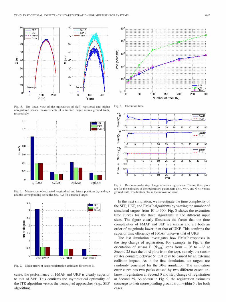
In the first simulation, ten targets are randomly generated inthe field-of-view of the sensors over a period of about 50 s. Weinitially set the registration parameters of the sensors randomlywith small numbers. Tracks are initialized using the zero-mean noninformative distributions. Fig. 5 shows the trajectoriesof unregistered measurements and an tracked target versusground truth. The red solid line represents the true trajectoryof the target, while the other blue solid, green dash-dotted, anddashed lines represent the fused results of the SEP, UKF, andFMAP algorithms, respectively. Fig. 6 shows the mean errors8

of position and velocity estimates of the target for the threealgorithms, respectively. The bar plot in Fig. 7 shows the meanerrors of the registration estimates for the three algorithms. Theperformance difference between UKF and FMAP is too smallto be seen on the scale used in the figures. Note that, in all the

7Rc = diag(εI, . . . , εI) and zc = [0, . . . , 0]T , where ε denotes a smallpositive number.

8The mean error is defined as ex = E{|x − xT |}, with x and xT being themeasurement and ground truth, respectively. Giving a series of measurementand truth pairs (xi, xTi), 1 ≤ i ≤ N , the sample mean error is computed as

ex =∑N

i|xi − xTi|/N .


Fig. 5. Top–down view of the trajectories of (left) registered and (right)unregistered sensor measurements of a tracked target versus ground truth,respectively.

Fig. 6. Mean errors of estimated longitudinal and lateral positions (eξ and eη)and the corresponding velocities (eξ, eη) for a tracked target.

Fig. 7. Mean errors of sensor registration estimates for sensor B.

cases, the performance of FMAP and UKF is clearly superiorto that of SEP. This confirms the asymptotical optimality ofthe JTR algorithm versus the decoupled approaches (e.g., SEPalgorithm).

Fig. 8. Execution time.

Fig. 9. Response under step change of sensor registration. The top three plotsare for the estimates of the registration parameters ξB0, ηB0, and ΨB0 versusground truth. The bottom plot is the innovation error.

In the next simulation, we investigate the time complexity ofthe SEP, UKF, and FMAP algorithms by varying the number ofsimulated targets from 10 to 300. Fig. 8 shows the executiontime curves for the three algorithms at the different inputsizes. The figure clearly illustrates the factor that the timecomplexities of FMAP and SEP are similar and are both anorder of magnitude lower than that of UKF. This confirms thesuperior time efficiency of FMAP vis-a-vis that of UKF.

The last simulation investigates how FMAP responses inthe step change of registration. For example, in Fig. 9, theorientation of sensor B (ΨB0) steps from −10◦ to −5◦ atSecond 25 (see the third plots from the top), namely, the sensorrotates counterclockwise 5◦ that may be caused by an externalcollision impact. As in the first simulation, ten targets arerandomly generated for the 50-s simulation. The innovationerror curve has two peaks caused by two different cases: un-known registration at Second 0 and step change of registrationat Second 25. As shown in Fig. 9, the registration estimatesconverge to their corresponding ground truth within 5 s for bothcases.


Fig. 10. (a) The test-bed vehicle equipped with two rangefinders. (b) Thesnapshot of a scene in the parking lot. (c) The top-down view of unregisteredrange data of the scene in (b). (d) The top-down view of registered range dataof the scene in (b).

IV. VEHICULAR EXPERIMENT

A test vehicle [Fig. 10(a)] equipped with two SICK LMS291rangefinders is used as the test bed to verify the effectivenessof the proposed FMAP. The two rangefinders are mounted attwo corners of the front bumper. The positions and orientationsof the rangefinders are precisely surveyed. The left rangefinder(sensor A) is located at (ξA0 = 3.724, ηA0 = 0.883), ori-ented 45◦ (ΨA0 = 45◦) outward from the vehicle’s boresight(ξ-coordinate). The right rangefinder (sensor B) is locatedat (ξB0 = 3.720, ηB0 = −0.874), oriented 45◦ (ΨB0 = −45◦)

outward from the vehicle’s boresight. The vehicle is alsoequipped with wheel encoders and an inertia measurement unit(IMU) sensor for determining the motion control inputs.

Each rangefinder is equipped with a point-object detector(e.g., tree trunks, light poles, etc.) that selects scan clusters suchthat 1) the size of the cluster is less than 0.5 m and 2) thedistance to the nearest point of other clusters is larger than5 m. The speed (i.e., range rate) of a point object is inferredfrom the host vehicle motion because of the stationary assump-tion of the point objects.

The experiment was conducted in a parking lot with plentyroad-side point objects shown in Fig. 10(b). The vehicle wasmanually driven, and an observation sequence of about 50 swas collected. The plot in Fig. 10(c) shows a snapshot ofunregistered range data for the scene in Fig. 10(b). The blackdots and magenta circles in the plot denote the scan datagenerated by the left and right rangefinders, respectively. Theblue circles and red stars denote the detected point objects fromthe left and right rangefinders, respectively.

The measurement inconsistence caused by the registrationbias is clearly seen. For example, the contours of the vehicle andthe point objects in Fig. 10(b) from the sensors are not aligned.The inconsistence raises an issue for data association. Without aconsistent registration, data from one sensor cannot be correctlyassociated with that from a different sensor. For comparison, thesnapshot of the registered range data of the same scene usingthe FMAP algorithm is shown in Fig. 10(d). The additionalblack diamonds in Fig. 10(d) denote the fused targets. Thisplot clearly reveals the fact that FMAP significantly improvesthe sensor registration and, thus, the data association amongmultiple sensors.

In each discrete time instant, the detected objects fromboth sensors are matched with the tracked targets [drawn asblack diamonds in Fig. 10(d)] at previous instant using anearest neighbor and a maximum distance gating data associ-ation strategy. We then apply the FMAP filter to jointly trackthe associated track–object pairs and registration parameters.Note that no target is visible in the whole observation se-quence. As shown in the last plot in Fig. 11, the dimensionof the state vector s changes due to new targets coming intoor existing targets leaving the field-of-view of the sensors.The method described in Section II-G is used to handle thechange.

In the experiment, the right rangefinder’s registration isunknown and initially set to (ξB0 = 2.720, ηB0 = −0.126,ΨB0 = −40◦). The SEP and FMAP algorithms are applied tothe data set. The resulted registration error curves for both algo-rithms versus the surveyed values are shown in Fig. 11(a). Theblue solid lines and the magenta dashed lines denote the errorcurves of SEP and FMAP, respectively. FMAP clearly exhibitssuperior performance comparing with that of SEP. As shownin Fig. 11(a), the estimates of the sensor’s position (ξB0, ηB0)and orientation ΨB0 converge to their true values in about 5 s,respectively. The slight transitory oscillation near the start ofthe run is partially due to the vehicle’s steering maneuver andlack of shared detected objects from both sensors. Better resultscan be obtained by incorporating vehicular motion model andglobal target map building. This may increase the computa-


Fig. 11. (a) Error curves of sensor registration estimates (ξB0, ηB0, andΨB0) for the right rangefinder when the true value is initially unknown.The last plot shows that the number of detected objects varies with time.(b) Corresponding mean errors for the registration estimates.

tional complexity of the algorithm. The fourth plot in Fig. 11(a)shows the number targets tracked by FMAP.

On the other hand, the significant mean registration error bythe SEP algorithm can be observed in Fig. 11(b). We shouldnote that the divergence of SEP curves increases over time inFig. 11(a), and this is partially contributed by the erroneous dataassociation caused by registration biases of previous cycles.Therefore, the estimates of registration by FMAP are moreconsistent and robust than that by SEP.

V. SUMMARY AND CONCLUSION

In this paper, we have addressed the recursive JTR. TheFMAP algorithm is derived in which the time complexityscales linearly with the numbers of measurements and targets.It is proved that FMAP is asymptotically optimal and has anO(n) implementation based on matrix orthogonal factorization.The results from experiments on synthetic and vehicular datademonstrate that, as expected, FMAP consistently performsbetter than the methods where tracking and registration are

separately treated. It has been also demonstrated experimentallyusing the synthetic data that the complexity of FMAP is indeedO(n). Although FMAP and UKF are quite equivalent in perfor-mance, the time complexity of FMAP is a magnitude lower thanthat of UKF. Additionally, the results of simulation and vehicleexperiment demonstrate that FMAP can handle the dynamics ofsensor registration and a variable number of targets.

APPENDIX

Lemma 6.1: Let ρ ∼ N (μρ,Σρ) or, in information arrayterms, [Rρ, zρ]. If ω = αρ + β, ω ∼ N (αμρ + β, αΣρα

t), orin information array terms, ω can be represented through[Rω, zω], where Rω = Rρα

−1 and zω = zρ + Rωβ.Proof: Since μρ = R−1

ρ zρ and Σρ = R−1ρ R−t

ρ , we get

μω =R−1ω zω = αμρ + β

Σω =R−1ω R−t

ω = αΣραt = αR−1

ρ R−tρ αt.

One can verify that Rω = Rρα−1 and

zω =Rωμω = Rω(αμρ + β) = Rω

(αR−1

ρ zρ + β)

=Rρα−1(αR−1

ρ zρ + β)

= (Rρα−1)

(αR−1

ρ

)zρ + (Rρα

−1)β

= zρ + (Rρα−1)β

= zρ + Rωβ.

�Lemma 6.2: Let the system dynamics be defined in (16),

the density function of the state variable s(t) = [x, a] be ex-pressed as information array in (14), and random noise termw be in information array form [Rw, zw]. Let ρ ≡ [w, s(t)]t.If w and s(t) are statistically independent, the joint densityof ω ≡ [w, x(t + 1), a(t + 1)]t can be represented through theinformation array [Rω, zω], where

Rω =

⎡⎣ Rw 0 0−RxΦ−1

x Gx RxΦ−1x Rxa

0 0 Ra

⎤⎦

zω =

⎡⎣ zw

zx + RxΦ−1x u2

za

⎤⎦ .

Proof: Since w and s(t) are statistically independent, theinformation array of the joint vector ρ = [w, s(t)]t = [w, x, a]t

is represented as [Rρ, zρ], where Rρ =

⎡⎣Rw 0 0

0 Rx Rxa

0 0 Ra

⎤⎦ and

zρ = [ zw zx za ]t.One verifies that the system dynamics equation (16) can be

reorganized as

ω = αρ + β


with α =

⎡⎣ I 0 0

Gx Φx 00 0 I

⎤⎦ and β =

⎡⎣ 0

u2

0

⎤⎦, and α−1 =

⎡⎣ I 0 0−Φ−1

x Gx Φ−1x 0

0 0 I

⎤⎦.

Using Lemma 6.1, we obtain

Rω = Rρα−1 =

⎡⎣ Rw 0 0−RxΦ−1

x Gx RxΦ−1x Rxa

0 0 Ra

⎤⎦

zω = zρ + (Rρα−1)β =

⎡⎣ zw

zx + RxΦ−1x u2

za

⎤⎦ .

�Lemma 6.3: Let ρ =

[ρ1

ρ2

]be distributed as ρ ∼ N (μρ,

Σρ) or information array [Rρ, zρ] with Rρ =[

Rρ11 Rρ12

0 Rρ22

]and z =

[zρ1

zρ2

]. Then, the marginal distribution of ρ2 is normal

and has ρ2 ∼ [Rρ22 , zρ2 ].Proof: By definition of information array, Σρ = R−1

ρ =[R−1

ρ11−R−1

ρ11Rρ12R

−1ρ22

0 R−1ρ22

]. Thus, the mean

μρ =R−1ρ zρ

=[

R−1ρ11

−R−1ρ11

Rρ12R−1ρ22

0 R−1ρ22

] [z1

z2

]

=[

R−1ρ11

zρ1 − R−1ρ11

Rρ12R−1ρ22

z2

R−1ρ22

zρ2

].

The marginal distribution of ρ2 ∼ N (μρ2 ,Σρ2), with μρ2 =R−1

ρ22zρ2 and Σρ2 = R−1

ρ22. Therefore, ρ2 ∼ [Rρ22 , zρ2 ]. �

REFERENCES

[1] A. Alempijevic, S. Kodagoda, and G. Dissanayake, “Sensor registra-tion for robotic applications,” in Field and Service Robotics. Berlin,Germany: Springer-Verlag, 2008, ser. Springer Tracts in AdvancedRobotics.

[2] I. Ashokaraj, P. Silson, A. Tsourdos, and B. White, “Robust sensor-basednavigation for mobile robots,” IEEE Trans. Instrum. Meas., vol. 58, no. 3,pp. 551–556, Mar. 2009.

[3] T. Bailey and H. Durrant-Whyte, “Simultaneous localization and map-ping: Part II,” IEEE Robot. Autom. Mag., vol. 13, no. 3, pp. 108–117,Sep. 2006.

[4] G. J. Bierman, Factorization Methods for Discrete Sequential Estimation.New York: Academic, 1977.

[5] R. Bishop, Intelligent Vehicle Technology and Trends. Norwood, MA:Artech House, 2005.

[6] S. Challa, R. Evans, X. Wang, and J. Legg, “A fixed-lag smoothing solu-tion to out-of-sequence information fusion problems,” Commun. Inf. Syst.,vol. 2, no. 4, pp. 325–348, Dec. 2002.

[7] E. D. Cruz, A. T. Alouani, T. R. Rice, and W. D. Blair, “Sensor registrationin multisensor systems,” in Proc. SPIE—Signal and Data Processing ofSmall Targets, Orlando, FL, 1992, pp. 1698–1703.

[8] U. Frese, “Simultaneous localization and mapping—A discussion,”in Proc. IJCAI Workshop Reason. Uncertainty Robot., Seattle, WA,Aug. 2001, pp. 17–21.

[9] D. Huang and H. Leung, “An expectation–maximization-based interactingmultiple model approach for cooperative driving systems,” IEEE Trans.Intell. Transp. Syst., vol. 6, no. 2, pp. 206–228, Jun. 2005.

[10] S. Jeong and J. Tugnait, “Tracking of two targets in clutter with possibleunresolved measurements,” IEEE Trans. Aerosp. Electron. Syst., vol. 44,no. 2, pp. 748–765, Apr. 2008.

[11] W. Li and H. Leung, “Simultaneous registration and fusion of multipledissimilar sensors for cooperative driving,” IEEE Trans. Intell. Transp.Syst., vol. 5, no. 2, pp. 84–98, Jun. 2004.

[12] X. Lin, Y. Bar-Shalom, and T. Kirubarajan, “Multisensor multitargetbias estimation for general asynchronous sensors,” IEEE Trans. Aerosp.Electron. Syst., vol. 41, no. 3, pp. 899–921, Jul. 2005.

[13] Y. Liu and S. Thrun, “Results for outdoor-slam using sparse extendedinformation filters,” in Proc. Int. Conf. Robot. Autom., Taipei, Taiwan,Sep. 14–19, 2003, pp. 1227–1233.

[14] R. Luo, C. Yih, and K. Su, “Multisensor fusion and integration:Approaches, applications, and future research directions,” IEEE SensorJ., vol. 2, no. 2, pp. 107–119, Apr. 2002.

[15] N. Okello and S. Challa, “Joint sensor registration and track-to-trackfusion for distributed trackers,” IEEE Trans. Aerosp. Electron. Syst.,vol. 40, no. 3, pp. 808–823, Jul. 2004.

[16] H. Ong, B. Ristic, and M. Oxenham, “Sensor registration using airlanes,”in Proc. 5th Int. Conf. Inf. Fusion, 2002, pp. 354–360.

[17] G. Rigatos, “Particle filtering for state estimation in nonlinear industrialsystems,” IEEE Trans. Instrum. Meas., vol. 58, no. 11, pp. 3885–3900,Nov. 2009.

[18] P. Tichavský, C. H. Muravchik, and A. Nehorai, “Posterior Cramér-Raobounds for discrete-time nonlinear filtering,” IEEE Trans. Signal Process.,vol. 46, no. 5, pp. 1386–1396, May 1998.

[19] J. Vermaak, S. Maskell, and M. Briers, “Online sensor registration,” inProc. IEEE Aerosp. Conf., Big Sky, MT, 2005, pp. 2117–2125.

[20] Y. Zhou, H. Leung, and P. C. Yip, “An exact maximum likelihood regis-tration algorithm for data fusion,” IEEE Trans. Signal Process., vol. 45,no. 6, pp. 1560–1573, Jun. 1997.

[21] S. Zeng and Y. Chen, “Joint tracking-registration with linear complexity:An application to range sensors,” in Proc. International Joint Conferenceon Neural Networks (IJCNN), Atlanta, GA, Jun. 2009, pp. 3498–3503.

Shuqing Zeng (M’03) received the Ph.D. degree incomputer science from Michigan State University,East Lansing, in 2004.

Since 2004, he has been with the Research andDevelopment Center, General Motors Corporation,Warren, MI, where he currently holds the positionof Senior Research Scientist. From 2005 to 2007,he served as the newsletter Editor of AutonomousMental Development TC, IEEE Computational Intel-ligence Society. He is currently an Associate Editorof International Journal Humanoid Robotics. His

research interests include computer vision, sensor fusion, autonomous driving,and active-safety applications on vehicle.

Dr. Zeng has served as a reviewer of the IEEE TRANSACTIONS ON PAT-TERN ANALYSIS AND MACHINE INTELLIGENCE and as a judge to IntelligentGround Vehicle Competition. He is a member of Tartan Racing team whowon the first place of the Defense Advanced Research Projects Agency UrbanChallenge on November 3, 2007.

fast optimal joint tracking–registration for multisensor systems

Documents