fast local approximation to global …wyman/publications/thesis/fastlocal...fast local approximation...
TRANSCRIPT

FAST LOCAL APPROXIMATION TO GLOBAL
ILLUMINATION
by
Christopher R. Wyman
A dissertation submitted to the faculty ofThe University of Utah
in partial fulfillment of the requirements for the degree of
Doctor of Philosophy
in
Computer Science
School of Computing
The University of Utah
August 2004

Copyright c© Christopher R. Wyman 2004
All Rights Reserved

THE UNIVERSITY OF UTAH GRADUATE SCHOOL
SUPERVISORY COMMITTEE APPROVAL
of a dissertation submitted by
Christopher R. Wyman
This dissertation has been read by each member of the following supervisory committeeand by majority vote has been found to be satisfactory.
Chair: Charles Hansen
Elaine Cohen
Victoria Interrante
Steven Parker
Peter Shirley

THE UNIVERSITY OF UTAH GRADUATE SCHOOL
FINAL READING APPROVAL
To the Graduate Council of the University of Utah:
I have read the dissertation of Christopher R. Wyman in its final formand have found that (1) its format, citations, and bibliographic style are consistent andacceptable; (2) its illustrative materials including figures, tables, and charts are in place;and (3) the final manuscript is satisfactory to the Supervisory Committee and is readyfor submission to The Graduate School.
Date Charles HansenChair, Supervisory Committee
Approved for the Major Department
Christopher R. JohnsonDirector
Approved for the Graduate Council
David S. ChapmanDean of The Graduate School
ABSTRACT
Interactive global illumination remains an elusive goal in rendering, as energy from
every portion of the scene contributes to the final image. Integrating over a complex
scene, with a polygon count in the millions or more, proves difficult even for static
techniques. Interacting with such complex environments while maintaining high quality
rendering generally requires recomputing the paths of countless photons using a small
number of CPUs. This dissertation examines a simplified approach to interactive global
illumination. Observing that local illumination computations can be performed inter-
actively even on fairly simple graphics accelerators, a reduction of global illumination
problems to local problems would allow interactive rendering. A number of techniques
are suggested that simplify global illumination to specific global illumination effects (e.g.,
diffuse interreflection, soft shadows, and caustics), which can individually be sampled
at a local level. Rendering these simplified global illumination effects reduces to a few
lookups, which can easily be done at interactive rates. While some tradeoffs exist between
rendering speed, rendering quality, and memory consumption, these techniques show
that approximating global illumination locally allows interactivity while still maintaining
significant realism.

CONTENTS
ABSTRACT . . . . . . . . . . . . . . . . . . . . . . . . . . . . . . . . . . . . . . . . . . . . . . . . . . . . . . iv
LIST OF FIGURES . . . . . . . . . . . . . . . . . . . . . . . . . . . . . . . . . . . . . . . . . . . . . . . vii
LIST OF TABLES . . . . . . . . . . . . . . . . . . . . . . . . . . . . . . . . . . . . . . . . . . . . . . . . . x
ACKNOWLEDGMENTS . . . . . . . . . . . . . . . . . . . . . . . . . . . . . . . . . . . . . . . . . . xi
CHAPTERS
1. INTRODUCTION . . . . . . . . . . . . . . . . . . . . . . . . . . . . . . . . . . . . . . . . . . . . . 1
1.1 Local Illumination . . . . . . . . . . . . . . . . . . . . . . . . . . . . . . . . . . . . . . . . . . . . 21.2 Global Illumination . . . . . . . . . . . . . . . . . . . . . . . . . . . . . . . . . . . . . . . . . . . 5
1.2.1 Radiometry . . . . . . . . . . . . . . . . . . . . . . . . . . . . . . . . . . . . . . . . . . . . . 51.2.2 Reflectance of Light . . . . . . . . . . . . . . . . . . . . . . . . . . . . . . . . . . . . . . 71.2.3 The Rendering Equation . . . . . . . . . . . . . . . . . . . . . . . . . . . . . . . . . . . 8
1.3 Motivation for Global Illumination . . . . . . . . . . . . . . . . . . . . . . . . . . . . . . . 81.4 Overview of this Work . . . . . . . . . . . . . . . . . . . . . . . . . . . . . . . . . . . . . . . . . 13
2. PREVIOUS WORK . . . . . . . . . . . . . . . . . . . . . . . . . . . . . . . . . . . . . . . . . . . 15
2.1 Radiosity Approaches . . . . . . . . . . . . . . . . . . . . . . . . . . . . . . . . . . . . . . . . . 162.2 Ray-based Approaches . . . . . . . . . . . . . . . . . . . . . . . . . . . . . . . . . . . . . . . . 172.3 Hybrid Radiosity-Raytraced Approaches . . . . . . . . . . . . . . . . . . . . . . . . . . 20
2.3.1 Interactive Hybrid Approaches . . . . . . . . . . . . . . . . . . . . . . . . . . . . . . 212.4 Soft Shadow Techniques . . . . . . . . . . . . . . . . . . . . . . . . . . . . . . . . . . . . . . . 222.5 Caustic Techniques . . . . . . . . . . . . . . . . . . . . . . . . . . . . . . . . . . . . . . . . . . . 262.6 Other Interactive Global Illumination Approaches . . . . . . . . . . . . . . . . . . . 27
3. INTERACTIVE SOFT SHADOWS USING PENUMBRA MAPS . . 31
3.1 Shadow Plateaus . . . . . . . . . . . . . . . . . . . . . . . . . . . . . . . . . . . . . . . . . . . . . 323.2 Penumbra Maps . . . . . . . . . . . . . . . . . . . . . . . . . . . . . . . . . . . . . . . . . . . . . 343.3 Implementation . . . . . . . . . . . . . . . . . . . . . . . . . . . . . . . . . . . . . . . . . . . . . . 39
3.3.1 Discussion of Limitations . . . . . . . . . . . . . . . . . . . . . . . . . . . . . . . . . . 403.4 Results . . . . . . . . . . . . . . . . . . . . . . . . . . . . . . . . . . . . . . . . . . . . . . . . . . . . . 41
4. INTERACTIVE RENDERING OF CAUSTICS . . . . . . . . . . . . . . . . . . 45
4.1 Caustics . . . . . . . . . . . . . . . . . . . . . . . . . . . . . . . . . . . . . . . . . . . . . . . . . . . . 474.1.1 Caustic Behavior . . . . . . . . . . . . . . . . . . . . . . . . . . . . . . . . . . . . . . . . . 474.1.2 Simplifying the Problem . . . . . . . . . . . . . . . . . . . . . . . . . . . . . . . . . . . 48
4.2 Caustic Sampling . . . . . . . . . . . . . . . . . . . . . . . . . . . . . . . . . . . . . . . . . . . . 494.2.1 Sampling the Light . . . . . . . . . . . . . . . . . . . . . . . . . . . . . . . . . . . . . . . 494.2.2 Sampling Space . . . . . . . . . . . . . . . . . . . . . . . . . . . . . . . . . . . . . . . . . . 50

4.2.3 Data Representation . . . . . . . . . . . . . . . . . . . . . . . . . . . . . . . . . . . . . . 514.3 Caustic Rendering . . . . . . . . . . . . . . . . . . . . . . . . . . . . . . . . . . . . . . . . . . . . 53
4.3.1 Rendering Algorithm . . . . . . . . . . . . . . . . . . . . . . . . . . . . . . . . . . . . . 534.3.2 Issues Rendering Caustic Data . . . . . . . . . . . . . . . . . . . . . . . . . . . . . . 54
4.4 Results . . . . . . . . . . . . . . . . . . . . . . . . . . . . . . . . . . . . . . . . . . . . . . . . . . . . . 574.5 Discussion . . . . . . . . . . . . . . . . . . . . . . . . . . . . . . . . . . . . . . . . . . . . . . . . . . 61
5. INTERACTIVE RENDERING OF ISOSURFACES WITH GLOBAL
ILLUMINATION . . . . . . . . . . . . . . . . . . . . . . . . . . . . . . . . . . . . . . . . . . . . . . 63
5.1 Background . . . . . . . . . . . . . . . . . . . . . . . . . . . . . . . . . . . . . . . . . . . . . . . . . 655.2 Overview . . . . . . . . . . . . . . . . . . . . . . . . . . . . . . . . . . . . . . . . . . . . . . . . . . . 665.3 Algorithm . . . . . . . . . . . . . . . . . . . . . . . . . . . . . . . . . . . . . . . . . . . . . . . . . . 70
5.3.1 Illumination Computation . . . . . . . . . . . . . . . . . . . . . . . . . . . . . . . . . . 705.3.2 Interactive Rendering . . . . . . . . . . . . . . . . . . . . . . . . . . . . . . . . . . . . . 73
5.4 Results . . . . . . . . . . . . . . . . . . . . . . . . . . . . . . . . . . . . . . . . . . . . . . . . . . . . . 74
6. CONCLUSIONS AND FUTURE WORK . . . . . . . . . . . . . . . . . . . . . . . . 85
APPENDICES
A. SHADER CODE FOR PENUMBRA MAPS . . . . . . . . . . . . . . . . . . . . . 88
B. SPHERICAL HARMONICS . . . . . . . . . . . . . . . . . . . . . . . . . . . . . . . . . . . . 93
REFERENCES . . . . . . . . . . . . . . . . . . . . . . . . . . . . . . . . . . . . . . . . . . . . . . . . . . . 110
vi

LIST OF FIGURES
1.1 Examples of local illumination models . . . . . . . . . . . . . . . . . . . . . . . . . . . . . . 3
1.2 The Phong illumination model uses four vectors to determine lighting foreach point . . . . . . . . . . . . . . . . . . . . . . . . . . . . . . . . . . . . . . . . . . . . . . . . . . . 4
1.3 Radiance is the energy per unit area per unit time per unit solid angle d~ω . 6
1.4 Renderings using local, direct, and global illumination . . . . . . . . . . . . . . . . . 10
1.5 An object’s shadow affects the perception of object location . . . . . . . . . . . . 11
1.6 Refraction of light through the cup and water introduces apparent bends,discontinuities, and other artifacts to a typical wooden pencil . . . . . . . . . . . 12
1.7 Common caustics from everyday life . . . . . . . . . . . . . . . . . . . . . . . . . . . . . . . 13
3.1 The shadow umbra includes regions where the light is completely occluded,and the penumbra occurs in regions where objects only partially occludethe light . . . . . . . . . . . . . . . . . . . . . . . . . . . . . . . . . . . . . . . . . . . . . . . . . . . . . 32
3.2 Penumbra maps in a scene with multiple lights . . . . . . . . . . . . . . . . . . . . . . . 33
3.3 Approximate soft shadows using shadow plateaus . . . . . . . . . . . . . . . . . . . . . 34
3.4 Rendering using penumbra maps . . . . . . . . . . . . . . . . . . . . . . . . . . . . . . . . . . 36
3.5 Explanation of penumbral sheets and cones . . . . . . . . . . . . . . . . . . . . . . . . . 37
3.6 Computing per-fragment intensity from cone or sheet geometry . . . . . . . . . . 37
3.7 Pseudocode for penumbra map fragment program . . . . . . . . . . . . . . . . . . . . 38
3.8 These pathtraced images show three different types of interactions betweenoverlapping penumbra . . . . . . . . . . . . . . . . . . . . . . . . . . . . . . . . . . . . . . . . . . 40
3.9 Penumbra map results for the Stanford bunny . . . . . . . . . . . . . . . . . . . . . . . 42
3.10 Penumbra map results for the dragon model . . . . . . . . . . . . . . . . . . . . . . . . . 43
4.1 A scene with caustics from a glass bunny . . . . . . . . . . . . . . . . . . . . . . . . . . . 46
4.2 The eight dimensions of a caustic . . . . . . . . . . . . . . . . . . . . . . . . . . . . . . . . . 48
4.3 Popping between adjacent light samples . . . . . . . . . . . . . . . . . . . . . . . . . . . . 50
4.4 Sampling space on either a uniform grid or a set of concentric shells . . . . . . 51
4.5 Sharper caustics come at the expense of denser sampling . . . . . . . . . . . . . . . 52
4.6 L intersects the spherical triangle formed by Li, Lj , and Lk . . . . . . . . . . . . 55
4.7 Ghosting happens when the caustic changes significantly between neighbor-ing light samples Li, Lj, and Lk . . . . . . . . . . . . . . . . . . . . . . . . . . . . . . . . . . 55

4.8 Alternative approach to caustic lookups . . . . . . . . . . . . . . . . . . . . . . . . . . . . 56
4.9 Caustic rendering techniques on a metal ring and glass cube . . . . . . . . . . . . 58
4.10 Caustic rendering techniques on a glass prism . . . . . . . . . . . . . . . . . . . . . . . 59
4.11 Casting caustics on complex objects . . . . . . . . . . . . . . . . . . . . . . . . . . . . . . . 60
4.12 The caustic of a prism in St. Peter’s cathedral using fifth order sphericalharmonics . . . . . . . . . . . . . . . . . . . . . . . . . . . . . . . . . . . . . . . . . . . . . . . . . . . . 60
5.1 Comparison of globally illuminated and Phong shaded isosurfaces . . . . . . . . 64
5.2 Computing the irradiance at point p involves sending a shadow ray andmultiple reflection rays . . . . . . . . . . . . . . . . . . . . . . . . . . . . . . . . . . . . . . . . . 67
5.3 The global illumination at each texel t is computed using standard tech-niques based on the isosurface I(ρ(xt)) through the sample . . . . . . . . . . . . . 68
5.4 The Visible Female’s skull globally illuminated using the new technique . . . 69
5.5 Pseudocode to compute irradiance at samples in the illumination lattice. . . 71
5.6 An isosurface from the Visible Female’s head extracted using analyticalintersection of the trilinear surface . . . . . . . . . . . . . . . . . . . . . . . . . . . . . . . . 72
5.7 Approaches to interpolating between illumination samples . . . . . . . . . . . . . . 74
5.8 The engine block illuminated by the Grace cathedral lightprobe . . . . . . . . . 76
5.9 An enlarged portion of the Richtmyer-Meshkov dataset shown in Figure 5.11 78
5.10 A Richtmyer-Meshkov instability simulation under various illumination . . . 79
5.11 Another view of a Richtmyer-Meshkov instability simulation . . . . . . . . . . . . 80
5.12 Comparison with vicinity shading . . . . . . . . . . . . . . . . . . . . . . . . . . . . . . . . . 81
5.13 The new technique versus Monte Carlo pathtracing with 10000 samples perpixel . . . . . . . . . . . . . . . . . . . . . . . . . . . . . . . . . . . . . . . . . . . . . . . . . . . . . . . . 82
5.14 Effect of different illumination volume resolutions . . . . . . . . . . . . . . . . . . . . . 83
A.1 Vertex program for rendering a penumbra map. . . . . . . . . . . . . . . . . . . . . . . 88
A.2 Fragment program for rendering a penumbra map. . . . . . . . . . . . . . . . . . . . . 89
A.3 Vertex program for rendering using a penumbra map. . . . . . . . . . . . . . . . . . 91
A.4 Fragment program for rendering using a penumbra map. . . . . . . . . . . . . . . . 92
B.1 Header file describing the SHRotationMatrix C++ class. . . . . . . . . . . . . . . . 104
B.2 Function definition for SHRotationMatrix::u i st(). . . . . . . . . . . . . . . . . . . . 105
B.3 Function definition for SHRotationMatrix::v i st(). . . . . . . . . . . . . . . . . . . . . 105
B.4 Function definition for SHRotationMatrix::w i st(). . . . . . . . . . . . . . . . . . . . 105
B.5 Function definition for SHRotationMatrix::U i st(). . . . . . . . . . . . . . . . . . . . 105
B.6 Function definition for SHRotationMatrix::V i st(). . . . . . . . . . . . . . . . . . . . 106
B.7 Function definition for SHRotationMatrix::W i st(). . . . . . . . . . . . . . . . . . . . 106viii

B.8 Function definition for SHRotationMatrix::P r i st(). . . . . . . . . . . . . . . . . . . 106
B.9 Function definition for SHRotationMatrix::R(). . . . . . . . . . . . . . . . . . . . . . . 106
B.10 Function definition for SHRotationMatrix::M(). . . . . . . . . . . . . . . . . . . . . . . 107
B.11 Function definition for SHRotationMatrix::matIndex(). . . . . . . . . . . . . . . . . 107
B.12 Definition of constructor SHRotationMatrix::SHRotationMatrix(). . . . . . . . 107
B.13 Function definition for SHRotationMatrix::computeMatrix(). . . . . . . . . . . . . 108
B.14 Function definition for SHRotationMatrix::applyMatrix(). . . . . . . . . . . . . . . 109
ix

LIST OF TABLES
1.1 Units of radiometric properties . . . . . . . . . . . . . . . . . . . . . . . . . . . . . . . . . . . 7
3.1 Framerate comparison using shadow and penumbra maps . . . . . . . . . . . . . . 41
4.1 Caustic rendering and precomputation times . . . . . . . . . . . . . . . . . . . . . . . . 57
5.1 Illumination computation timings for images from Figure 5.8 . . . . . . . . . . . 75
5.2 Comparison of framerates and memory consumption for Figure 5.8 . . . . . . . 77
B.1 Definitions of numerical coefficients uis,t, vi
s,t, and wis,t. . . . . . . . . . . . . . . . . . 102
B.2 Definitions of the functions U is,t, V i
s,t, and W is,t. . . . . . . . . . . . . . . . . . . . . . . . 102
B.3 Definitions of the function rPis,t. . . . . . . . . . . . . . . . . . . . . . . . . . . . . . . . . . . 102

ACKNOWLEDGMENTS
I would like to thank everyone who helped and supported me during my graduate
work. In particular, my advisor Chuck Hansen deserves thanks for funding and enabling
my research as well as his helpful comments and discussion along the way. Pete Shirley
also provided immense help and guidance during my tenure in Utah; I would particularly
like to thank him for sharing his vast rendering knowledge and keeping the lab amused
with his unique sense of humor.
I would also like to thank my other committee members, Steve Parker, Elaine Cohen,
and Vicki Interrante, for interesting discussions, scheduling flexibility, and useful feedback
on my work.
My colleagues in the Graphics and SCI labs helped keep me sane during long nights in
the lab, provided insightful feedback on my work, and entertained me outside the lab. In
no particular order, I would like to thank Shaun Ramsey, Dave DeMarle, Charles Schmidt,
Rahul Jain, Aaron Lefohn, Milan Ikits, Joe Kniss, Mike Stark, Bill Martin, Erik Reinhard,
Simon Premoze, Helen Hu, Rose Mills, Margarita Bratkova, Justin Polchlopek, Kristi
Potter, Bruce Gooch, Amy Gooch, Dylan Lacewell, Dave Edwards, and Joel Daniels.
Outside of the department, I met many people in Utah who kept me from becoming
too focused on work. Particularly, all the people I met through various band organizations
in the Music Department helped keep my musical abilities alive. I would also like to thank
them for all the opportunities they afforded me, including the chance to participate in
the 2002 Winter Olympic Games.
Finally, I would like to acknowledge my family, and particularly my parents, for
the support they have given throughout my educational career. They had unwaivering
confidence in my abilities, even when I had doubts.
This work was supported by the National Science Foundation under Grants 9977218
and 9978099 as well as the College of Engineering’s Wayne Brown Fellowship. Addition-
ally, portions of Chapter 3, including figures and tables, are reprinted with permission
from my 2003 paper [152] from the Eurographics Symposium on Rendering, copyright
the Eurographics Association for Computer Graphics.

CHAPTER 1
INTRODUCTION
Computer graphics involves creating, or rendering, images of synthetic environments.
Often the goal is to render images of these environments as realistically as possible.
Achieving images indistinguishable from photographs, called photorealistic images, re-
quires accurate physical models of light transport, complex materials, and geometry.
Although object geometry is relatively easy to simulate given the right primitives, mod-
eling light transport and complex material properties are areas of active research. This
dissertation examines ways to simplify complex illumination so interactive applications
can benefit from improved realism.
In part due to the complex illumination present in real world environments, photo-
realistic renderings of environments remain difficult to generate using computer graphics
techniques. This difficulty arises because illumination requires global information. Light
bounces off virtually all objects, so computing the color at some point in a scene involves
integrating over all the incident illumination. Obviously, such an operation can prove
extremely time consuming. Even after 30 years of research, code optimization, and
dramatically improved computer processors, such illumination computations still prove
expensive. Because of this expense, realistic renderings are usually generated by batch
processes and interactive applications continue to use lower quality lighting approxima-
tions.
Over the past 30 years, assorted models have been proposed for simulating illumination
for computer graphics. Initially, objects were drawn in wire-frame [4, 80]. Later models
like flat, Gouraud [40], and Phong [102] shading use local information at every point
on the object to determine illumination. These models provide only local illumination.
Raytracing techniques [149] and rasterization techniques like shadow mapping [25] ex-
tended illumination models to allow direct illumination, which includes shadows when
objects occlude the light. Illumination arriving directly from a light, without bouncing
off intermediate objects, is called direct illumination.

2
More recent illumination models approximate the rendering equation [67], allowing
inclusion of indirect illumination—light reflected off other objects in the environment.
The rendering equation models the physical transport of light through a scene, and was
borrowed from the study of radiative heat transfer. Because solutions to the rendering
equation require global knowledge of the scene, such as geometry and material properties,
the resulting illumination is called global illumination.
Often the terms local and direct illumination are used interchangeably. However, local
lighting relies on local information such as position, surface normal, viewing direction,
and direction to the light. Hence, purely local models cannot achieve shadowing effects,
which require knowledge about global visibility. Direct illumination, on the other hand,
includes all the light directly hitting a surface. In cases where the light is hidden by an
occluder, a surface will not be illuminated. Similarly, global and indirect illumination
are often interchanged. Indirect illumination is a subset of global illumination, but the
shadowing effects of direct illumination models also require global visibility information.
Computing local lighting is easy because it requires only local information. Thus,
interactive applications such as simulators, architectural walkthroughs, computer-aided
design programs, and computer games usually rely on local illumination models. While
current techniques are vastly better than the interactive methods of a decade ago, due
to the improved computation power available on graphics hardware, most interactive
techniques still lack complex global lighting effects seen in the real world. Thus, only
applications that can afford slow computations, such as special-effects and computer
generated movies, enjoy the fruits of decades of global illumination research.
1.1 Local Illumination
Early computer graphics researchers focused their efforts on the most important
problems of the time, namely techniques to render geometry quickly. Generally, they
used simple empirical illumination models such as the flat, Gouraud, and Phong shading
techniques shown in Figure 1.1. These techniques are composed of three parts: an
ambient term which approximates indirect illumination, a diffuse term that approximates
matte materials, and a specular term which adds a specular, or glossy, appearance.
Because these local models ignore indirect illumination, the user-defined ambient term
helps brighten surfaces not directly illuminated. This gives renderings a more realistic
appearance.
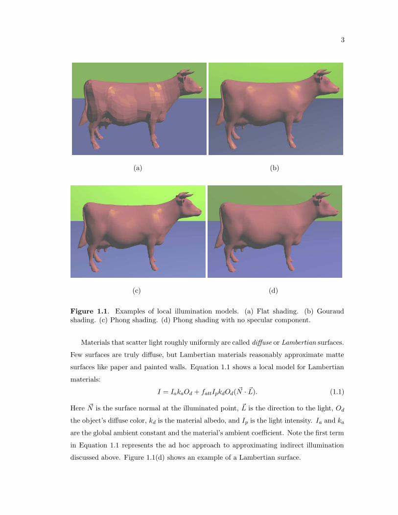
3
(a) (b)
(c) (d)
Figure 1.1. Examples of local illumination models. (a) Flat shading. (b) Gouraudshading. (c) Phong shading. (d) Phong shading with no specular component.
Materials that scatter light roughly uniformly are called diffuse or Lambertian surfaces.
Few surfaces are truly diffuse, but Lambertian materials reasonably approximate matte
surfaces like paper and painted walls. Equation 1.1 shows a local model for Lambertian
materials:
I = IakaOd + fattIpkdOd( ~N · ~L). (1.1)
Here ~N is the surface normal at the illuminated point, ~L is the direction to the light, Od
the object’s diffuse color, kd is the material albedo, and Ip is the light intensity. Ia and ka
are the global ambient constant and the material’s ambient coefficient. Note the first term
in Equation 1.1 represents the ad hoc approach to approximating indirect illumination
discussed above. Figure 1.1(d) shows an example of a Lambertian surface.
4
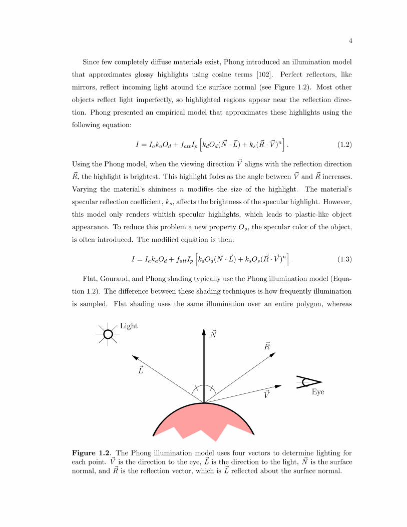
Since few completely diffuse materials exist, Phong introduced an illumination model
that approximates glossy highlights using cosine terms [102]. Perfect reflectors, like
mirrors, reflect incoming light around the surface normal (see Figure 1.2). Most other
objects reflect light imperfectly, so highlighted regions appear near the reflection direc-
tion. Phong presented an empirical model that approximates these highlights using the
following equation:
I = IakaOd + fattIp
[
kdOd( ~N · ~L) + ks(~R · ~V )n]
. (1.2)
Using the Phong model, when the viewing direction ~V aligns with the reflection direction
~R, the highlight is brightest. This highlight fades as the angle between ~V and ~R increases.
Varying the material’s shininess n modifies the size of the highlight. The material’s
specular reflection coefficient, ks, affects the brightness of the specular highlight. However,
this model only renders whitish specular highlights, which leads to plastic-like object
appearance. To reduce this problem a new property Os, the specular color of the object,
is often introduced. The modified equation is then:
I = IakaOd + fattIp
[
kdOd( ~N · ~L) + ksOs(~R · ~V )n]
. (1.3)
Flat, Gouraud, and Phong shading typically use the Phong illumination model (Equa-
tion 1.2). The difference between these shading techniques is how frequently illumination
is sampled. Flat shading uses the same illumination over an entire polygon, whereas
~V
Light
Eye
~N
~R
~L
Figure 1.2. The Phong illumination model uses four vectors to determine lighting foreach point. ~V is the direction to the eye, ~L is the direction to the light, ~N is the surfacenormal, and ~R is the reflection vector, which is ~L reflected about the surface normal.

5
Gouraud samples the illumination at all polygon vertices and linearly interpolates the
results for a smoother effect. Phong shading interpolates the normals over the polygon
and performs lighting computations on a per-pixel basis. As seen in Figure 1.1, Phong
shading allows highlights to span less than a single triangle, whereas Gouraud shading
often spreads highlights over multiple triangles or misses them completely.
The models presented in this section run interactively and are easy to implement, but
they cannot represent many of the complex effects seen in everyday environments. Shad-
ows, reflections, interreflections, and caustics all require global information. Technically,
area lights can be handled using local illumination models, but the approaches used in
interactive applications typically handle only point lights.
1.2 Global Illumination
Global illumination provides much of the visual richness in typical real-world environ-
ments. For instance, indoor environments and star-lit night renderings are often almost
exclusively lit by indirect illumination. Unfortunately, incorporating global information
about all objects in an environment proves quite costly. In fact, generating photorealistic
images requires solving the rendering equation [67] introduced by Kajiya, which models
the physical transport of light. Solving this equation proves costly because it involves
integrating incoming illumination recursively at every point in a scene. In fact, computa-
tion of exact solutions are feasible only in the simplest environments. Renderers generally
use a numerical approximation technique to solve this integral.
Kajiya’s formulation of the rendering equation computes the intensity arriving at some
point x from some other point x′ in the environment via the following equation:
I(x,x′) = g(x,x′)
(
ε(x,x′) +
∫
x′′∈S
ρ(x,x′,x′′)I(x′,x′′)dx′′)
. (1.4)
The illumination arriving at point x from point x′ depends on the visibility, g(x,x′),
between x and x′, the light emitted, ε(x,x′), from x′ to x, and a sum of the illumination
incident at x′ reflected towards x. Here ρ(x,x′,x′′) describes how much light from x′′ is
reflected towards x at point x′.
1.2.1 Radiometry
Kajiya’s rendering equation provides a framework to compute global illumination, but
rendering photorealistic images also requires accurate knowledge about an environment’s
lighting. The most pragmatic approaches to obtain physically accurate data are to either

6
measure light intensities in a real environment or allow users to input intensities in
common, human-understandable units. In either case radiometry, the measurement of
real-world radiation, proves useful. By rewriting the rendering equation in terms of
radiometric properties, physical measurements can easily be incorporated into simulated
environments.
The most basic radiometric property, radiant energy, has units of joules. Radiant flux,
Φ describes the radiant energy Q per unit time t, or Φ = dQdt . The commonly used unit
for radiant flux is the watt. Radiant flux area density represents the radiant flux per unit
area. Radiant flux area density is called irradiance, represented as E, when discussing
power arriving at a surface and is called radiosity, represented as B, when referring to
power leaving a surface. More explicitly:
E(x) =dΦin
dA, (1.5)
B(x) =dΦout
dA. (1.6)
The radiance, L, is defined as the energy per unit area per unit time per unit solid
angle, or the radiant flux area density per unit solid angle. Given the radiant flux at point
x in area dA from some direction d~ω (see Figure 1.3), the radiance can be computed as
x
~ωθ
dA
~N
d~ω
Figure 1.3. Radiance is the energy per unit area per unit time per unit solid angle d~ω.If the area dA lies along a surface at point x with surface normal ~N , the radiance iscomputed using the projected area cos θdA.

7
follows:
L(x, ~ω) =d2Φ
cos θdAd~ω, (1.7)
where cos θdA is the projected area of dA to the plane perpendicular to the direction ~ω.
As an example, the energy radiated in the angle d~ω from the region dA during time dt
in Figure 1.3 can be computed:
Q = L(x, ~ω) cos θdAd~ωdt.
Table 1.1 summarizes the physical units of the radiometric properties introduced in this
section.
1.2.2 Reflectance of Light
Another important property to consider when rendering photorealistic images is how
light interacts with materials in a scene. Every material reflects light in a slightly differ-
ent manner, depending on composition, age, translucency, and the microscopic surface
geometry. Until the introduction of the rendering equation, however, most materials used
in computer graphics were approximated by purely Lambertian models, purely specular
models (i.e., perfect reflectors or refractors), or the Phong model, which gives a plastic
appearance with varying specular highlights.
As more complex rendering techniques became widespread, a better representation
for material properties was needed. A more realistic approximation for reflected light
is the bidirectional reflectance-distribution function, or BRDF, introduced by Nicodemus
et al. [91]. The BRDF represents the portion of light from an incoming direction ~ωin
that reflects in a particular outgoing direction ~ωout, hence it can represent surfaces with
arbitrary reflectances. Cook and Torrance [24] and Immel et al. [57] first discussed
the bidirectional reflectance in the computer graphics literature, and Cabral et al. [14]
introduced the standardized notation of Nicodemus et al. Formally, the BRDF, fr, is
Table 1.1. Units of radiometric properties.Symbol Property Units
Q Radiant energy JΦ Radiant flux WE Irradiance Wm−2
B Radiosity Wm−2
L Radiance Wm−2sr−1

8
defined as the ratio of outgoing radiance to the irradiance from the incident direction
~ωin:
fr(x, ~ωout, ~ωin) =dL(x, ~ωout)
dE(x, ~ωin)=
dL(x, ~ωout)
L(x, ~ωin) cos θind~ωin. (1.8)
The BRDF approximates the reflectance of a material, but as a function independent
of surface location it cannot represent effects such as subsurface scattering and translu-
cency. Nicodemus et al. also introduced the bidirectional scattering-surface reflectance-
distribution function, or BSSRDF, a more general function than the BRDF which allows
such effects. While the BSSRDF still only encompasses a subset of all radiative trans-
fer [17], it allows transfer from all geometrical optics effects. Jensen et al. [66] recently
introduced a subsurface scattering model based on the BSSRDF.
1.2.3 The Rendering Equation
Using the radiometric properties from Section 1.2.1 and the reflectance discussed in
Section 1.2.2, the rendering equation can be rewritten to allow use of physically based
measurements. More explicitly, the rendering equation computes an outgoing radiance
from a surface based on the light emitted by the surface, the incident radiance, and the
surface’s material properties. Mathematically, this can be written [57]:
Lout(x, ~ωout) = Lemit(x, ~ωout) +
∫
Ωfr(x, ~ωout, ~ωin)Lin(x, ~ωin) cos θind~ωin, (1.9)
where Lemit is the radiance emitted from x in direction ~ωout, Ω is the visible hemisphere
at x, fr is the BRDF, and θin is the angle between ~ωin and the surface normal ~N at x.
An interesting property of radiance is that it remains constant along a line in space,
assuming no intervening surfaces. So, assuming no surface exists between x and x + α~ω,
L(x, ~ω) = L(x + α~ω, ~ω),∀α ∈ R.
Because of this property, the outgoing radiance at x, Lout(x, ~ω), is equal to the incoming
radiance at x′, Lin(x′,−~ω), if x′ is the closest surface along the line x + α~ω. Utilizing
this property, the rendering equation (Equation 1.9) becomes a recursive equation that
can be solved to compute a full global illumination solution.
1.3 Motivation for Global Illumination
Comparing the complexity of models described in Sections 1.1 and 1.2, global il-
lumination obviously requires significantly more computation than the commonly used

9
local illumination models. Considering the extra resources needed for global illumination,
several important questions need to be considered. What effects does global illumination
allow that local illumination does not? How important are the effects that global illumi-
nation captures? And can these global illumination computations be simplified and still
capture the same important effects?
Local illumination models assume light interacts with every surface facing the source
and restrict light to interact with a single surface. Thus, local illumination renders
images without shadows, reflections, color bleeding, refractions, or the focusing of light.
Moreover, local models typically assume light originates from point sources, so rendering
outdoor scenes illuminated by the entire sky is impossible. Such effects are all common
in real environments, hence for applications placing a high priority on realism the extra
computation time for global illumination is worthwhile. Figure 1.4 shows the importance
of a few of these global effects.
Experiments have shown shadows play an important role in human perception. Ker-
sten et al. [71] showed that fake shadows can cause illusory motion in stationary objects.
Further work by Kersten et al. [72] found an object moving along a set trajectory can
appear at different depths depending on shadow location. People attach an object to its
apparent shadow when determining relative locations, as shown in Figure 1.5. Accurate
spatial perception may not rely on accurate shadows [144], but adding them to a synthetic
scene improves both the spatial cues and the realism. For instance, changing shadow
size, position, or orientation in an image can cause occluders to change apparent size or
location [145]. A number of experiments have shown shadows provide important contact
cues in virtual environments [56, 81].
Reflections provide other useful information in real environments. Interior designers
commonly use mirrors to make rooms appear larger than their actual size [103, 104].
Diffuse reflections, also called color bleeding or interreflections, can be used for a similar
effect. Painting the walls of a room white, which increases the light reflected between adja-
cent walls, also makes a room seem larger [103, 104]. Besides allowing similar perceptions
in synthetic environments, reflections also play important roles in the appearance of many
materials, especially those with significant specular coefficients. Some research suggests
interreflections may provide spatial cues similar to those provided by shadows [81]. Ad
hoc planar mirrored reflections are straightforward to add to locally illuminated scenes;
however, reflections off curved objects are difficult [94] and lead to major artifacts without

10
(a) (b)
(c) (d)
Figure 1.4. Renderings using local, direct, and global illumination. (a) Local lightingonly. (b) Direct lighting using a point light source. (c) Globally illuminated scene. (d)Globally illuminated scene with metallic (instead of Lambertian) buddha. Notice theother walls of the room have green and purple tints, which can be seen in the diffuseinterreflections on the model in (c).

11
(a) (b)
Figure 1.5. An object’s shadow affects the perception of object location. These twoimages are identical, except for shadow size and location.
utilizing global illumination techniques.
No studies have examined the effect of refractions on human perceptions in computer
generated renderings, yet they do add significantly to the realism of a scene. Objects
seen through refractive objects like magnifying glasses, textured windows, or bodies of
water can appear dramatically different from the same object seen without the refraction
(see Figure 1.6). The focusing of light by reflective or refractive surfaces, called a caustic,
provides similar realism. For instance, the caustic at the bottom of a coffee cup or caused
by a magnifying glass (see Figure 1.7) may or may not provide important perceptual
information, but images without such caustics lack realism. Similarly, light focused by the
water in a swimming pool forms caustics on the pool floor. As a common effect, renderings
without underwater caustics look distinctly odd, hence films and video games frequently
approximate such caustics using texture maps to help enhance realism [60, 127, 128].
In the real world, only objects with finite extent emit light. However, many interactive
computer graphics applications model light sources as infinitesimal points. Using point
light sources leads to illumination inaccurate in many ways. For instance, shadows have
hard, crisp edges as visibility between two points is a binary function. Real light sources
can be partially occluded, resulting in smoother soft shadows. Area light sources result in
quite complex illumination as direct light arrives from a variety of directions. In addition,
representing lights as spherical environment maps allows the use of lighting captured from
real environments [26]. This use of natural lighting conditions has been found to improve
the perceived realism of an image in certain circumstances [100, 110], though this topic

12
Figure 1.6. Refraction of light through the cup and water introduces apparent bends,discontinuities, and other artifacts to a typical wooden pencil. Also note the woodentable top visible in refractions where it would otherwise not appear.

13
(a) (b)
(c) (d)
Figure 1.7. Common caustics from everyday life. (a) A cardioid at the bottom of acoffee cup. (b) Light focused on the bottom of a pool by the surface. And light focusedthrough (c) a magnifying glass and (d) an acrylic juggling ball.
remains the subject of active research.
These global illumination effects all provide significant amounts of realism to computer
generated scenes, but studies have shown that accuracy does not matter in all cases [144].
Furthermore, it may be unnecessary to accurately portray interreflections, refractions, or
caustics as long as the results appear plausible.
1.4 Overview of this Work
The major obstacle to using global illumination in interactive applications is the
significant computational resources required for accurate results. Many studies have
shown that global illumination effects provide important perceptual cues, yet they find

14
that perfect illumination is usually unnecessary and in some cases even physically im-
plausible illumination may be acceptable. This suggests techniques which simplify global
illumination via approximation could render images most users accept as real.
As current interactive applications extensively utilize local illumination techniques,
the approach suggested in this dissertation is to store global illumination approximations
locally. With global information stored at a local level, global illumination computations
simplify to lookups followed by simple computations (such as interpolation) over these
local values. Such an approach easily extends current interactive techniques to add more
complex lighting. This dissertation examines local ways to independently approximate
three different global effects: soft shadows, caustics, and diffuse interreflections. The
approaches for soft shadows and caustics rely on commonly used polygonal datasets,
whereas the work on diffuse interreflection focuses on volumetric datasets used in visual-
ization applications.
Chapter 2 discusses the goals and drawbacks of previous work in global illumination
and interactive techniques. Chapter 3 examines a technique for rendering plausible
approximations to soft shadows using penumbra maps [152], Chapter 4 describes an
approach for generating interactive caustics dynamically [153], and Chapter 5 introduces
a method for globally illuminating isosurfaces dynamically extracted from volumetric
datasets. Finally, conclusions and future work are discussed in Chapter 6.

CHAPTER 2
PREVIOUS WORK
Researchers have long examined techniques to render more realistic illumination.
Early empirical models such as Phong [102], Blinn [11], and Whitted [149] illumination
were augmented by more realistic techniques such as the Cook-Torrance model [24]. The
Cook-Torrance model incorporates additional information, such as the solid angle the
light subtends, the slope distribution of microscopic surface facets, and the Fresnel term,
which describes how surface reflectance varies based upon illumination angle, extinction
coefficient, and index of refraction. The Cook-Torrance model renders objects more
realistically than earlier empirical models, but it still relies only on local information, and
thus misses many important illumination effects.
Two basic approaches emerged for computing global lighting: radiosity and raytracing.
Radiosity [38] builds on ideas from radiative heat transfer [17] to model diffuse interactions
between Lambertian surfaces. This allows color-bleeding to occur between nearby objects
and easily incorporates the effects of uniform area lights. An additional benefit is that
computed radiosities are viewpoint independent, so viewers can interactively move about
a static scene without recomputing the solution. Unfortunately, radiosity is based upon
energy transfer between discrete regions, so solutions are constant over these finite regions.
This leads to aliasing and interpolation artifacts unless a scene is highly tessellated, in
which case computation times can become prohibitive.
Raytracing shoots rays from the cemera into the scene. These rays intersect scene
objects to determine which surfaces are visible in a given direction. Whitted [149]
extended the basic idea to a recursive raytracer, where rays need not terminate once
they hit a surface. Instead, should a ray intersect a specular surface, it continues on in
the reflected or refracted direction.
The remainder of this chapter discusses numerous categories of related work in render-
ing. Sections 2.1, 2.2, and 2.3 respectively discuss research related to radiosity, raytracing,

16
and hybrid radiosity-raytracing techniques. Sections 2.4 and 2.5 introduce research on
interactively rendering two specific global illumination effects: soft shadows and caustics.
2.1 Radiosity Approaches
The basic radiosity approach [8], introduced to computer graphics by Goral et al. [38],
associates a form factor with each pair of patches in a scene. The form factor specifies
what percentage of the outgoing energy from the first patch hits the second. Using these
form factors, a large linear system can be solved to compute the radiosity at each patch.
Cohen and Greenberg [22] introduced the hemi-cube method for computing form factors
between patches in a complex scene. By projecting scene geometry onto an imaginary
cube centered on a patch, visibility information is stored in the form factor, allowing one
patch to occlude portions of the light traveling between other patches.
Further work on radiosity techniques has focused on three areas: easing the restriction
to exclusively diffuse materials, increasing accuracy, and speeding up the computations,
either for the original solution or for dynamic scenes.
Immel et al. [57] extended standard radiosity to allow specular materials. Instead
of storing a single radiance, each patch stores a directional radiance for a variety of
incoming and outgoing directions. This allows surfaces with specular properties to be
precomputed. Just like in diffuse radiosity, the solution is view-independent, even though
view-dependent specular effects are captured. Unfortunately, with specular surfaces
interpolation artifacts over patches become much more noticeable, particularly as the
eyepoint moves. Additionally, since all patches are planar, curved surfaces are handled
poorly.
Until Cohen et al. [21] introduced progressive radiosity, solutions were completely
computed before display could begin. Progressive radiosity shoots energy progressively,
one patch at a time, instead of solving the entire system of linear equations defined
by a scene’s form factors. This allows incremental display of the scene as computation
progresses, albeit with initially coarse estimates.
Chen [19] described a method called incremental radiosity, which extends progressive
radiosity to allow changes to scene properties between iterations. Thus, increasing or
decreasing a light’s brightness shoots incremental positive or negative light into the scene.
Changing geometry involves removing energy (or shooting negative energy) contributed
by the object in its former location, and adding energy contributed from the new loca-

17
tion. Hence, scenes can dynamically change during computations without necessitating
a complete recomputation. Unfortunately, such changes can noticeably affect the scene,
and propagating the changes through the radiosity solution often requires significant
time, especially for dramatic changes in light intensity. In most interactive applications,
where scenes continuously change, incremental radiosity never converges and can lead to
objectionable lighting artifacts.
As interpolation across patches causes significant artifacts in radiosity-based render-
ings, a number of researchers have proposed techniques for reducing these artifacts.
Hanrahan et al. [46] used a hierarchical quad-tree approach to adaptively subdivide
patches as needed. Accordingly, areas where radiance changes quickly become finely
subdivided. Hanrahan et al. also used this hierarchy to estimate form factors based on
interactions between large patches. This reduces the standard O(n2) radiosity technique,
which computes interactions between all n patches in the scene, to O(n).
Interpolation artifacts still occur in hierarchical radiosity, as patches do not coincide
with discontinuities in the illumination. Lischinski et al. [78] combined hierarchical
radiosity with discontinuity meshing [50, 51, 77] to create patches which coincide with
illumination discontinuities, such as shadow boundaries. Gortler et al. [39] generalized
the idea of hierarchical radiosity by introducing wavelet radiosity, and work by Zatz [154]
and Troutman and Max [134] explored the idea of representing radiosity by non-constant,
higher order functions to reduce interpolation artifacts.
Radiosity techniques poorly capture specular effects and converge slowly, particularly
in dynamic environments. However, when combined with the ray-based approaches
described in Section 2.2, these techniques provide much of the basis for more recent
interactive global illumination techniques.
2.2 Ray-based Approaches
The recursive raytracing technique introduced by Whitted [149] is an easily imple-
mentable, elegant approach to shading objects. Distributed raytracing [23] extends the
idea to allow reflecting or refracting in a variety of directions, based on material properties.
In effect, this allows a Monte Carlo sampling [89] of the material BRDF at intersection
points. As most surfaces do not reflect or refract perfectly (like a mirror or window pane),
distributed ray tracing allows much more realistic material properties. Additionally, by
distributing rays over time, an area light, or a camera lens, effects such as motion blur,

18
soft shadows, and depth-of-field can be rendered. Kajiya and Von Herzen [68] extended
raytracing to handle volumes such as smoke, dust, or clouds via multiple sampling of
scattering functions over the volumes.
Kajiya [67] showed that all these raytracing techniques solved a subset of a more gen-
eral illumination problem posed by the rendering equation (discussed in Section 1.2.3). He
proposed a new approach, called pathtracing, which solved Equation 1.9 by Monte Carlo
integration. A path describes the motion of a photon through reflections, refractions, and
scattering from the light to the eye. Sampling numerous paths at every pixel in an image
thus computes a full global illumination solution, with bounded error for each pixel. The
results are quite compelling; however, large numbers of paths are required before images
converge. Using fewer samples results in noisy images, particularly in regions containing
complex paths to luminaires, like caustics.
One approach to accelerate pathtracing involves reducing path variance so that fewer
samples per pixel are necessary for good results. Arvo and Kirk [7] discuss the tradeoffs
between terminating rays early via Russian roulette and splitting rays at intersections.
Spawning new rays can reduce variance by concentrating work in regions most sensitive
to noise, but it can also focus more work at leaves of the ray tree, where contributions are
minimal. Russian roulette stochastically terminates rays early, as if a surface absorbed
the photon. This reduces the total number of rays, at the cost of slightly higher variance.
One reason for high variance in pathtraced images is the varying number of bounces
before a light is hit. By combining rays cast from the eye with photons emitted from the
light, bidirectional pathtracing [74] reduces variance by using each intersection on the light
path as an emitter for points on the eye path. Considering the importance of particular
paths [31, 32, 101, 123], both from the eye and the light, allows reduced numbers of
paths in regions less important to the rendering, which allows higher sampling rates and
reduced variance in important regions.
Observing that illumination frequently changes slowly and gradually over space, with
occasional discontinuities, also suggests that caching illumination values and interpolating
over relatively constant regions could significantly reduce the frequency at which expen-
sive illumination computations must be performed. Ward et al. [146] demonstrated that
such caching techniques provide significant savings for pathtracers.
The areas in a pathtraced image with greatest variance result from specular interac-
tions. For instance, caustics are formed when light from specular objects focuses in one

19
small area. The paths of light causing these effects are often convoluted and difficult to
sample tracing only rays from the eye. Arvo [6] suggested emanating photons from the
light and storing them in illumination maps located on Lambertian surfaces. Using this
technique, paths need not randomly bounce around numerous times before accidentally
reaching a light source. Instead, at each diffuse surface, a simple lookup provides the
incident illumination. Heckbert [49] proposed adaptively subdividing these illumination
maps based on photon density and regions of importance, such as shadow boundaries.
The bidirectional pathtracing of Lafortune and Willems [74] also extended this approach.
Jensen [64] introduced the concept of a photon map. Instead of storing a texture
of irradiance values, as in an illumination map, the photons themselves are stored,
usually in a kd-tree. When computing incident illumination at a point, contributions
from the n-nearest photons are averaged. Since photon mapping does not use discrete
texels, fewer photons are necessary to eliminate noise. Extensions to the photon map use
importance to determine where to shoot photons [61], allow more efficient soft shadow
rendering [63], eliminate the requirement for diffuse receivers [62], and allow interaction
with participating media [65].
Photon mapping reduces the number of paths and photons to render complex specular
effects, such as caustics, yet large numbers of photons are still required. In the case of
dynamic scenes, recomputation must occur after every object movement or change of
material property. Purcell et al. [105] implemented a basic photon mapping scheme on
graphics hardware in an attempt for quicker rendering. Due to limitations of graphics
cards, their implementation uses a simple grid-based storage scheme for photons instead
of a kd-tree, reducing caustic reconstruction quality. Additionally, their approach requires
a number of seconds per frame, even for simple scenes.
Bala et al. [10] stored sampled radiance in a linetree, which is the four-dimensional
equivalent of an octree. By interpolating and reprojecting these sampled radiances when
encountering similar rays, the costs of raytracing are significantly reduced. In addition,
they provided bounds on the resulting errors so image fidelity can be maintained at
any desired level. Radiance interpolants can provide a significant speedup over standard
raytracing approaches; however, in areas where radiance varies quickly, such as in caustics,
artifacts may be difficult to eliminate.
A number of approaches utilize coherency to speed up rendering times. Beam trac-
ing [52] traces beams instead of individual rays. As adjacent rays typically hit nearby
20
surfaces, a single intersection can save significant computation. Veach and Guibas [136]
mutated existing paths in a Monte Carlo pathtracer. Once an important path is found,
mutated paths generally significantly contribute to the image as well. Recently, Chen and
Arvo [18] examined perturbations of specular paths to accelerate computation of specular
reflections.
2.3 Hybrid Radiosity-Raytraced Approaches
Both radiosity and ray-based approaches have advantages. Pathtracing captures any
global illumination effect, albeit at great cost, whereas radiosity progressively computes
view-independent diffuse solutions. Numerous researchers have examined techniques of
combining these approaches to get the benefits of each while reducing variance and
computation time.
Wallace et al. [140] proposed a two-pass approach. In the first pass, a radiosity
solution is computed that stores diffuse to diffuse surface interactions and specular to
diffuse interactions. The second pass uses a distributed raytracing approach to compute
specular to specular and diffuse to specular interactions. Sillion and Puech [118] extended
this two-pass approach to allow multiple specular interactions along a light path and
eliminate the restriction limiting specular objects to planar patches.
Malley [82] and Maxwell et al. [85] proposed using raytracing to compute form factors
between patches. By casting rays out from a patch, accurate form factors to other patches
can be computed, even with complex occluding geometry. Wallace et al. [141] turned this
around and gathered light at patch vertices via ray casting, which allowed smoother
interpolation over patches.
Shirley [114] proposed a three-pass process that first shoots photons from luminaires
via illumination mapping, then computes diffuse interreflections using a modified radiosity
approach (which ignores direct lighting), and finally traces rays from the eye and performs
direct lighting computations. This approach easily captures complex effects like caustics,
unlike most earlier methods.
Chen et al. [20] extended hybrid approaches to provide user feedback during rendering,
and allow elimination of most interpolation artifacts from the radiosity steps. Using an
initial progressive radiosity pass with nondiffuse form factors computed using ray tracing,
the most important effects are seen quickly. A second pass using pathtracing computes
shadows and caustics, although computations focus only on bright objects that cause

21
such effects. A final pass uses per-pixel pathtracing to remove interpolation artifacts
from the initial radiosity solution. This final pathtracing pass uses the radiosity solution
for secondary reflections, so path lengths are kept short.
Keller [70] introduced a quasi-Monte Carlo approach that sends out particles from
the light. Where these particles hit scene geometry, virtual lights are placed which also
illuminate the scene. Accumulating direct lighting results from the virtual point lights and
samples on area lights allows approximate global illumination to be computed on hardware
graphics accelerators relatively quickly. Extensions allow simple specular effects, but they
also increase the number of hardware passes needed for convergence. The complexity of
Keller’s approach is linear in both light samples and scene complexity. Unfortunately, for
high quality renderings, these values are not independent. As scene complexity increases,
more samples may be required for accurate illumination reconstruction.
2.3.1 Interactive Hybrid Approaches
The hybrid approaches discussed so far attempted to reduce rendering time of photo-
realistic results, but a number of hybrid approaches took the opposite approach: keeping
interactive rendering speeds while still achieving as much realism as possible.
George et al. [37] provided a mechanism to update an existing progressive radiosity
solution as changes occur in a dynamic environment. Before an object moves, negative
energy is emitted from its patches, to counteract the energy it contributed to the current
solution. After movement, positive energy is directed at it from important patches in the
scene to relight the object in its new location. A similar approach can handle changing
material properties.
Forsyth et al. [36] suggested a link hierarchy building on the hierarchical radiosity
algorithm [46]. Links between patches can either become occluded, or need “promo-
tion” or “demotion” between levels of the hierarchy. By using predictive link tests and
extrapolation, they can compute radiosity interactively in simple scenes.
Smits et al. [122] grouped patches in a scene into clusters, which could interact on a
cluster level, rather than the patch level. This allows objects that have little effect on each
other to interact at a higher level, which reduces computational costs. They described
two approaches to bound the error this clustering technique introduces. Depending on
the acceptable approximation error, the O(n2) radiosity computation reduces to either
O(n log n) or O(n).

22
Drettakis and Sillion [30] combined clustering with an approach similar to Forsyth et al.
During object motion, intersections between the object’s bounding volume and existing
links are computed. Their technique expedites radiosity computations, but interactive
framerates are limited to fairly simple scenes.
Granier et al. [42] proposed another approach using hierarchical radiosity with clus-
tering for the diffuse pass, and utilizing particle tracing for specular effects. Particles
contribute to surfaces based on the hierarchy, which allows acceleration of visibility
computations during path tracing. Granier and Drettakis [41] extend this approach,
constructing caustics directly on the radiosity mesh or in a “caustic texture,” depending
on required accuracy. Furthermore, they include the line-space hierarchy of Drettakis
and Sillion, allowing interactive modification of the scene. However, as with most particle
tracing systems their approach works best with relatively simple scenes. The number of
paths necessary for high quality increases dramatically as scene complexity increases.
2.4 Soft Shadow Techniques
Significant research has focused on creating a unified global illumination technique
that renders complete illumination at interactive rates, yet other research has focused
on more specific problems. Interactive raytracing-radiosity hybrids have potential, but
most current applications cannot afford the expense they entail. More specific techniques,
which focus on soft shadows for example, can quickly be applied in applications, as they
are simpler than complete solutions.
Since shadows can significantly improve image comprehension, researchers have long
examined techniques to incorporate them into existing applications that use only lo-
cal illumination. Crow [25] proposed an object-space solution to compute simple hard
shadows. The extrusions of an object’s silhouettes away from the light bound the
shadowed region. Computing shadow volumes, these silhouettes and their polygonal
extrusions, allows analytic computation of hard shadows for polygonal models. Another
early technique introduced by Williams [150] computed shadows using an image-based
approach. By storing distances to the objects nearest the light in a shadow map, objects
further away can be correctly occluded. Because of the simplicity of shadow volumes
and shadow maps, these techniques are the most widely used approaches in interactive
applications, especially as both techniques are easily adaptable to acceleration on graphics
hardware [53, 113]. Woo et al. [151] and Akenine-Moller and Haines [3] have surveyed

23
early shadow techniques and discussed their relative advantages and disadvantages.
A number of interesting extensions to these basic techniques have been introduced.
Reeves et al. [109] introduced percentage closer filtering, which helps eliminates shadow
map aliasing along shadow boundaries. Percentage closer filtering renders shadows with
soft boundaries. However, this blur is proportional to a fixed parameter and does not
vary with light size or distance between receiver and occluder. McCool [86] developed a
hybrid approach which generates shadow volumes from shadow maps. McCool’s approach
does not render soft shadows, but its use may become widespread as graphics accelerators
become more powerful and can implement the process independent of the CPU.
Shadow mapping and shadow volumes quickly render hard shadows. However, they
do not allow generation of soft shadows, except by sampling the light many times and
accumulating the result (suggested by Heckbert and Herf [48]). As with most sampling-
based integral approximations, this approach requires many samples to avoid artifacts,
which in this case manifest as banding. For typical scenes, at least 64 samples per light
are necessary for smooth shadows. Even with modern graphics accelerators, rendering a
scene an additional 64 times per frame proves prohibitive.
A number of approaches speed exact soft shadow computation. Drettakis and Fi-
ume [29] and Steward and Ghali [132] used backprojection to compute a discontinuity
mesh. Using backprojection of objects onto light sources, regions of the scene where light
occlusions have similar structure are computed. A discontinuity mesh represents the
boundaries of these regions on scene geometry. Using this approach dramatically reduces
clipping costs for computing light visibility.
Stark and Riesenfeld [130] reformulated Lambert’s formula for computing irradiance.
The original formula sums over the edges of a polygon while the reformulation sums over
vertices. By tracing vertices onto the image plane, this new formulation can exactly
compute accurate shadows for polygonal scenes. The algorithm quickens shadow compu-
tations, yet it fails to accelerate the process enough for use in interactive applications.
Although exact shadow computations are possible to quickly compute for simple
scenes with polygonal sources and occluders, they slow dramatically as scene complexity
increases. Thus, many researchers have investigated approximate approaches for ren-
dering soft shadows. Soler and Sillion [125, 126] computed approximate soft shadows
by convolving an image of the light source with a projected image of the occluders.
Unfortunately, their approach required lights and occluders to occupy parallel planes,

24
which rarely happens in real-world situations. As positions of lights and occluders diverge
from parallel planes their approximation breaks down, and for very complex geometry
the artifacts are quite obvious without error reduction techniques that drastically increase
computation time. Additionally, this approximation breaks down as occluders approach
receivers, where the shadow should become sharp.
Another image-based method, suggested by Agrawala et al. [1], samples the light,
renders the scene for each sample, and warps these images into a layered depth image.
In some ways this approach is similar to simply sampling the light many times, as scene
geometry still must be rendered 64 or more times to compute accurate layered depth
images. Agrawala et al. also discussed a number of approaches to speeding up this
precomputation, but their results still require minutes of computation for complex scenes.
In environments with dynamic geometry or illumination, such precomputation speeds are
unacceptable.
An algorithm developed by Heidrich et al. [54] renders approximate soft shadows from
a linear light source. At samples along the light, shadow maps are computed. Using image
warping techniques, visibility percentages are computed for each point in the shadow
maps. This value represents the percentage of the light seen from that location in the
scene. This process can be costly for complex scenes, especially when more than two or
three samples on the light are used. Additionally, a number of situations exist where
artifacts occur and the technique limits scenes to two-dimensional lights.
Ouellette and Fiume [95] proposed projecting occluders onto the light, using an algo-
rithm to find discontinuities along the edges of the light source, and using discontinuity
locations to approximately determine the portion of the light occluded. The results
are compelling, but projecting all objects onto every light source quickly becomes cost
prohibitive, especially since nontriangular sources must be subdivided, with the projection
process being repeated on each subdivided, triangular light.
Hart et al. [47] lazily computed visibility information. As a first pass, cast rays
determine visible geometry. Shadow rays spawned in a uniform pattern at intersections
determine some occluders. Using a flood-fill algorithm, neighboring pixels are checked to
determine if the same blockers also occlude nearby regions. A second pass computes
illumination for each pixel based on the blockers found during the first pass. This
approach can provide significant speedups over Monte Carlo visibility evaluation at each
pixel, but it has a number of problems. First, it is not designed for interactivity. Worse,

25
when objects are subdivided into many small triangles, each triangle casts only a very
small shadow, which could easily be missed with only a few shadow rays per pixel. In
such a case, a pixel deep in an umbral region may be only partially occluded.
Haines [45] introduced a technique which quickly renders a shadow texture on a
plane. This technique approximates umbral regions using a hard shadow, and extends
these regions with approximate penumbrae. Parker et al. [99] suggested this approach of
extending hard shadows by approximate penumbral regions. Haines’ approach generates
plausible soft shadows when occluders lie relatively close to the shadowed plane, and is
discussed further in Section 3.1.
Brabec and Seidel [12] described a technique for computing soft shadows using an
image-space search of a single shadow map. If the shadow map shows a pixel as il-
luminated, a pixel-by-pixel search conducted in nearby regions of the shadow map de-
termines whether the pixel lies in a penumbral region. Similarly if the shadow map
shows a blocker occluding the pixel, a search of nearby shadow map texels determines
if the pixel is partially illuminated. The results provide acceptable shadows quickly,
but stepping artifacts appear in penumbral regions and artifacts occur near overlapping
objects. Additionally pixel-by-pixel searches currently must be performed on the CPU.
The illumination computation for each pixel includes such a search, so this process can
become costly, especially as the shadow map size increases.
Akenine-Moller and Assarsson [2] extended the shadow volume approach to render
soft shadows. Instead of computing a single shadow quadrilateral at each silhouette
edge, a penumbra wedge that surrounds the penumbral region is computed in addition
to the shadow quadrilateral. A per-fragment shader program renders these wedges
into a light buffer, used during the final illumination pass. The problems with this
technique include assuming silhouettes form closed loops with exactly two silhouette
edges per vertex, requiring a 16-bit stencil buffer for use as the light buffer, and increased
bandwidth requirements for the additional penumbra wedge geometry. An extension to
this technique [9] eliminated most of these problems and allowed for colored area lights.
However, the bandwidth limitation restricts the complexity of objects casting shadows.
Even on state of the art graphics hardware, simple scenes (with a few hundred polygon
occluders) render at only a few frames per second.

26
2.5 Caustic Techniques
Although the problem of rendering caustics has not received as much attention as soft
shadow rendering, a number of researchers have proposed techniques for interactively
rendering caustics. As with soft shadows, the hybrid raytracing-radiosity approaches can
interactively render caustics for very simple objects, but more complex objects require
significantly more time.
Watt [147] described a variant of beam tracing [52] called light beam tracing. In
beam tracing, bundles of rays, or beams, are used instead of single rays. Using beams
reduces computation time by utilizing coherency information between nearby rays which
intersect the same surface. Watt’s light beam tracing shoots beams from the light, instead
of individual photons. Each specular polygon in the scene is the base of a pyramidal
light beam, with the apex at the light. These light beams can individually be reflected
and refracted by specular polygons with a single transformation, rather than on a per-
photon basis. This allows much quicker computation of caustics through a single specular
interaction. Problems with the beam tracing approach include the limitation to a single
specular interaction, which limits the applicability, and the need to highly tessellate
curved surfaces in order to achieve realistic results.
Mitchell and Hanrahan [88] introduced a technique for directly computing the caustic
intensity from a reflecting implicit surface. Their approach uses results from geometric
optics that describe the energy in a spherical wavefront and how the wavefront interacts
with reflective and refractive materials. Instead of a ray-surface intersection problem,
their approach locates ellipsoid-surface tangencies. The results have few discretization
artifacts, but they limit themselves to implicit surfaces and single specular interactions.
Finally, their technique requires significant computational resources.
Nishita and Nakamae [92] combined metaball surfaces with illumination volumes
(essentially light beams refracted by a single surface) using Z-buffers, A-buffers, and
shadow volumes to render caustics on underwater curved objects. In addition, they
handle underwater scattering effects, giving visible “shafts” of light. Like most previous
techniques, this approach allows only single-interaction caustics, namely caustics from a
light-water interaction, limiting the applicability to a small subset of real-world caustics.
Furthermore, because each illumination volume must be recomputed and rasterized each
frame, similar to a shadow volume, the cost prohibits dynamic caustics.
Stam [127] suggested dynamically computing underwater caustics may be unneces-

27
sary, as an approximation stored in a series of texture maps generates plausible results.
Combining this approach with aperiodic texture mapping [128] noticeably reduces the
periodicity resulting from a short series of caustic textures.
Diefenbach and Badler [28] utilized graphics hardware to render approximate global
illumination effects quickly. They proposed using light volumes, analogous to shadow
volumes, to bound regions where additional light should be added. These volumes are
similar to refracted light beams and can be rasterized using the same stencil method [53]
used for shadow volumes. Light volumes can be recursively generated as they intersect
second specular surfaces. This approach does not directly render caustics, but when
combined with explosions maps [94] to reflect from curved surfaces, caustic generation
may be possible. Unfortunately, this approach is very fragile and requires significant
fill rate (for multiple recursive shadow and light volumes). Even without caustics, this
multi-pass pipeline approach requires multiple seconds per frame.
Wand and Straßer [143] proposed using recent programmability of graphics accelera-
tors to render caustics. Using a pixel shader for every pixel P in the scene, they sample
points S on a specular surface, reflect−−−→S−P around the normal at S, and index into a
cube map of the surrounding environment. By sampling the surface numerous times,
they perform Monte Carlo sampling of a single-bounce caustic. With current hardware,
they performed three samples per rendering pass. This allows interactive framerates
for a few samples per pixel (from 60–500), though caustics often require one or two
orders of magnitude more samples for crisp results. However, for simple metallic objects
where blurry caustics are acceptable, their approach runs interactively on current graphics
accelerators.
2.6 Other Interactive Global IlluminationApproaches
While hybrid radiosity-raytracing techniques and specialized approaches for specific
effects have materialized, a number of other interesting techniques have been introduced.
Greger et al. [44] introduced the irradiance volume which allows dynamic objects to
traverse an environment and allows nearby geometry to illuminate them via diffuse
interreflection. The environment is sampled on a grid and an approximation to the
irradiance function is stored in each cell. Interpolation between samples allows dynamic
objects to be illuminated by the scene, however dynamic objects cannot affect illumination
of static geometry.

28
A number of approaches have achieved interactivity via brute force. Raytracing
algorithms are embarrassingly parallel, meaning they scale linearly as additional CPUs
are added to a computation. Parker et al. [96] implemented an interactive raytracer
on a multiprocessor SGI Origin. Using 60 CPUs, a combination of good acceleration
structures, load balancing, memory bricking, and code optimization allowed interactive
framerates for fairly complex scenes. A similar interactive raytracing technique was in-
troduced by Wald et al. [139] which uses clusters of commodity PCs to achieve interactive
speeds. The approach of Wald et al. takes advantage of SIMD streaming instructions
on modern commodity CPUs, reduces all objects to triangle primitives, and carefully
monitors network traffic to maintain interactivity.
Wald et al. [138] extended their work to render scenes with global illumination at
interactive rates. Because of a limit on rays per frame, a number of assumptions were
made to expedite rendering. Instead of randomly sampling the lights at each pixel, a set
number of predetermined light samples are used. In order to eliminate the structured
noise resulting from this sampling, the raytracer uses a discontinuity buffer to smooth
irradiance over nearby pixels. Caustics are computed using a photon map stored in a
grid instead of a kd-tree, for faster creation and lookups. While this improved approach
allows interactive global illumination, 5 × 5 pixel blocks are blurred together by the
discontinuity buffer, which causes blurred caustics and noise along object boundaries. By
performing an approximate importance sampling, they showed [137] that light samples
can be intelligently chosen, even in complex environments with thousands of lights.
Walter et al. [142] introduced the render cache, which caches previous illumination
computations and reprojects them as a user interacts with the environment. By reusing
and reprojecting existing illumination samples, new rays and paths can be concentrated
in regions that significantly change between frames. The render cache also allows frames
to be generated asynchronously, rather than waiting for all illumination computations at
every pixel on screen. The render cache allows interactivity without shooting rays for
every pixel (similar to the approach of [10]), but high quality results require a number of
frames, and artifacts and blurriness occur in regions of movement and near discontinuities.
Udeshi and Hansen [135] combined hardware acceleration and raytracing to achieve re-
alistic effects like soft shadows, one bounce diffuse interreflections, and specular reflections
in dynamic environments. Using a parallel SGI Origin with eight Infinite Reality graphics
pipelines, shadows and direct illumination were computed using the graphics hardware,

29
and raytracing on the CPUs gave accurate specular reflections. They approximated
indirect illumination by rerendering the scene from virtual lights.
A number of recent techniques have explored compressing and storing global lighting
using various basis functions. Generally these techniques rely on incident illumination
from infinitely distant light sources, so that lighting remains constant over objects in the
scene. Ramamoorthi and Hanrahan [106] applied spherical harmonics to environment
maps to compress them to nine coefficients for each of the red, green, and blue channels.
Rendering requires a simple matrix multiply followed by a dot product to accurately
illuminate Lambertian materials with direct light from the environment. Programmable
graphics hardware can easily implement this approach, and with third order spherical
harmonics per-pixel error remains below three percent. Ramamoorthi and Hanrahan [108]
extended their work to allow rendering of more complex, isotropic BRDFs by combining
precomputed illumination coefficients with precomputed BRDF coefficients. By assuming
a distant viewpoint (in addition to distant illumination), the spherical harmonic functions
can be evaluated only once per frame instead of once per pixel, allowing for interactive
rendering.
Sloan et al. [120] introduced precomputed radiance transfer, which allows interactive
integration of incident illumination and precomputed coefficients describing radiance
transfer within a single object. This approach allows interreflections, self-shadowing
and low frequency caustics. Both the incident illumination and precomputed radiance
transfer are represented using spherical harmonic coefficients. Observing that integration
of two functions projected into the same spherical harmonic basis simplifies to a simple
dot product of coefficient vectors, the illumination integral of Equation 1.9 simplifies to
a few multiplies and adds, which they implement using programmable pixel shaders for
interactive rendering. The results are impressive for diffuse materials, yet caustics are
poorly represented because they require high frequency information eliminated by the
projection of the environment map into a spherical harmonic basis. Additionally, in order
for nearby objects to contribute to each other’s illumination, they must remain stationary
relative to each other. Radiance transfer for more complex materials must be represented
by a matrix of coefficients rather than a single vector, so non-Lambertian materials signifi-
cantly slow rendering times. Sloan et al. [121] extended this work to allow a combination of
surface microgeometry with precomputed radiance transfer. Sloan et al. [119] compressed
the spherical harmonic transfer coefficients using a variety of approaches, allowing for

30
high quality rendering of specular materials with fewer coefficients. Additionally, they
extended the transfer function to permit subsurface scattering effects. Using newer
graphics cards with extended functionality, this new approach renders interactively for
dynamic illumination and viewpoint.
Ng et al. [90] suggested using a nonlinear wavelet basis instead of a spherical harmonic
basis. Because wavelets have local, instead of global, support, they can compactly rep-
resent high frequency illumination in addition to low frequency lighting. They projected
each row of the transfer matrix into a Harr wavelet basis, quantized the elements to eight
bits, and discarded any zero coefficients, allowing for a sparse transfer matrix. As with
the approach of Sloan et al., this approach requires static geometry, as recomputing the
transfer matrix is expensive.

CHAPTER 3
INTERACTIVE SOFT SHADOWS USING
PENUMBRA MAPS
Shadows provide cues to important spatial relationships. By changing shadow size,
position, or orientation in an image, an object can appear to change size or location [145].
Similarly, soft shadows give contact cues. As an occluder approaches a shadowed object,
its soft shadow becomes sharper. When objects touch the shadow is completely hard.
Many recent interactive applications have incorporated real-time shadows, but they
generally use shadow volumes [25], shadow maps [150], or related techniques. These
methods use point light sources that cast only hard shadows. Since real world lights
occupy not a point but some finite area, photorealistic images require soft shadows. Thus,
as interactive graphics systems become more realistic, methods for quickly rendering soft
shadows are needed.
Shadows consist of two parts, an umbra and a penumbra. Umbral regions occur
where a light is completely occluded from view and penumbrae occur when a light
is partially visible (Figure 3.1). Until very recently the only techniques to compute
these regions involved either evaluating complex visibility functions [47] or merging hard
shadows rendered from various points on the light [48]. Evaluating visibility is slow,
and sampling techniques produce banding artifacts unless many samples are used. Other
approximations have emerged, but most do not allow dynamically moving objects to
shadow arbitrary receivers.
This chapter introduces the penumbra map [152], which allows arbitrary polygonal
objects to dynamically cast approximate soft shadows onto themselves and other arbitrary
objects. A penumbra map augments a standard shadow map with penumbral intensity
information. Shadows rendered using this approach (see Figure 3.2) harden when objects
touch, avoid banding artifacts inherent in sampling schemes, and are generated interac-
tively using commodity graphics hardware. Additionally, penumbra maps can leverage
existing research on shadow maps (e.g. perspective shadow maps [129] or adaptive

32
(a) (b)
Figure 3.1. The shadow umbra includes regions where the light is completely occluded,and the penumbra occurs in regions where objects only partially occlude the light.Hard shadows (a) have only an umbra, whereas soft shadows (b) have both umbral andpenumbral regions.
shadow maps [35] to help reduce shadow aliasing). On the other hand, the penumbra
map approach breaks down when the umbra region shrinks significantly or completely
disappears. This happens for very large area light sources or when an occluder shadows
distant objects.
The next section describes related work on shadow plateaus, followed by a discussion of
the penumbra map algorithm in Section 3.2. Section 3.3 discusses some implementational
specifics and outlines the limitations. Section 3.4 presents the results.
3.1 Shadow Plateaus
Recent work by Haines [45] proposed a technique for generating approximate soft
shadows on a ground plane using “plateaus.” Haines’ method creates a texture containing
intensity which is used to modulate the local illumination at points on the plane to
approximate a shadow. This approach first projects geometry onto the plane from
the center of a light, as in Figure 3.3(a), giving a standard hard shadow, and then
extends the hard shadow by an approximation to the penumbral regions, similar to the
work of Parker et al. [99]. To draw these approximate penumbrae, polygons attached

33
(a) (b)
Figure 3.2. Penumbra maps in a scene with multiple lights. With two penumbra maps(a), this scene runs at 21.6 fps for 1024x1024 images. Compare to shadow maps (b) whichonly render hard shadows.

34
to the silhouette edges of occluding geometry, similar to the shadow quads used for
shadow volumes, are projected into the shadow texture with varying intensity based on
distance to the ground plane. First, cones based at the ground plane with apexes at
silhouette vertices are rendered (Figure 3.3(b)). Usually these cones are discretized into
triangles for quick rendering via acceleration on graphics cards. Finally, the cones are
connected by hyperboloid sheets attached to silhouette edges and tangent to adjacent
cones (Figure 3.3(c)). When the adjacent cones have differing radii, the connecting sheet
is nonplanar. As OpenGL and DirectX introduce artifacts when rasterizing nonplanar
quadrilaterals, these sheets are subdivided into smaller triangles.
When rendered into the shadow texture, these cones and sheets have intensities of
zero, for fully shadowed, at silhouette edges and one, for fully illuminated, at the ground
plane. For locations in between the ground and the silhouette, the intensity is interpolated
either linearly or sinusoidally, as proposed Parker et al. [99].
3.2 Penumbra Maps
Shadow plateaus give compelling shadows quickly enough for use with dynamic occlud-
ers, but this approach cannot shadow arbitrary surfaces. However, since people are often
poor judges of soft shadow shape [144], similar plausible soft shadows should suffice in
interactive environments. The penumbra map technique extends Haines’ shadow plateau
(a) (b) (c)
Figure 3.3. Approximate soft shadows using shadow plateaus. The shadow plateautechnique generates soft shadows by (a) first rendering a hard shadow, (b) renderingcones at each silhouette vertex, (c) rendering sheets connecting the cones.

35
work to allow dynamic soft shadows on arbitrarily complex objects.
Two observations form the basis for the penumbra map technique. First, a shadow
map can easily create the hard shadow to approximate an umbra. Second, if one assumes
this hard shadow approximates the umbra, then the entire penumbra is visible from the
point on the light used for the hard shadow. This allows the penumbra information to
be stored in a single texture called a penumbra map. This texture stores the penumbral
intensity on the foremost polygons visible from the light, just as a shadow map stores
depth information about these surfaces. These observations led to similar, concurrent
work by Chan and Durand [16], allowing them to render approximate soft shadows using
new geometric primitives called smoothies.
Rendering with penumbra maps is a three-pass process. The first pass renders a
standard shadow map from the viewpoint of a point light source at the approximate
center of the light. The second pass renders the penumbra map. The third pass combines
depth information from the shadow map and intensity information from the penumbra
map to render the final image.
Let V ≡ v1, v2, . . . and E ≡ e1, e2, . . . be the set of silhouette vertices and edges,
as seen from the light. Let Lr be the light radius, Zvithe depth value of vertex vi from
the light, and Zfar be the distance to the light’s far plane. Then, to generate a penumbra
map (such as in Figure 3.4):
• Clear the penumbra map to white.
• Find V and E for the current light.
• ∀vi ∈ V, draw a cone with tip at vi and base at the far plane (see Figure 3.5) with
a radius at the base of Cri=
(Zfar−Zvi)Lr
Zvi. Subdivide each cone into a number of
triangles with one vertex at vi and two on the far plane.
• ∀ei ∈ E , draw a sheet connecting adjacent cones. Depending on the cone radii, this
quad may be nonplanar. Subdivide extremely nonplanar quads to avoid artifacts.
Every pixel in the penumbra map corresponds to a pixel in the shadow map. Each
penumbra map pixel stores the shadow intensity at the corresponding surface in the
shadow map. A fragment program applied to the penumbra sheets and cones computes
this intensity using the simple geometry shown in Figure 3.6. The idea is that by using
Zvi, the depth of the current cone or sheet fragment ZF , and depth of the corresponding

36
(a) (b)
(c)
Figure 3.4. Rendering using penumbra maps. (a) An example shadow map, (b) thecorresponding penumbra map, and (c) the final rendered result.

37
OccluderPenumbra Cone
Far Plane
Light Radius Lr
Zvi
Zfar
Cone Radius Cri
(a)
Light
Occluder
Far Plane
Penumbra Sheet
PenumbraCone
(b)
Figure 3.5. Explanation of penumbral sheets and cones. (a) Each cone’s tip is locatedat a vertex vi with the base located at the far plane. Simple geometry allows computationof the cone radius Cri
. (b) Each sheet connects two adjacent cones.
Edge of penumbra
Zvi
Light
Far Plane
Receiver
Occluder
P
F
ZF
ZPEdge of umbra
using this method
Figure 3.6. Computing per-fragment intensity from cone or sheet geometry. Eachfragment F corresponds to some surface location P visible in the shadow map. By usingZvi
, ZF and ZP , the intensity I is computed via Equation 3.1.

38
shadow map pixel ZP , one can compute the light intensity at point P. Equation 3.1
specifies this computation:
I = 1 − ZP − ZF
ZP − Zvi
=ZF − Zvi
ZP − Zvi
. (3.1)
The CPU computes Zvion a per-vertex basis. For cones Zvi
is constant, and for sheets
the graphics card’s rasterizer interpolates between the Zvivalues of the two adjacent
cones. ZP can be computed by referencing the shadow map, and ZF is automatically
computed by the rasterizer when processing fragment F .
This process gives a linear intensity gradient through approximate penumbral regions.
Parker et al. [99] note that for spherical lights this intensity should vary sinusoidally. They
approximate this sinusoidal falloff using the Bernstein interpolant s = 3τ 2 − 2τ3. The
results presented in Section 3.3 use this approximation, with the same assumption of
spherical light sources.
Figure 3.7 contains pseudocode for a fragment program to compute the penumbra
map (Appendix A contains the actual vertex and fragment programs). Since both the
shadow map, Smap, and the penumbra map are rendered with the same viewing matrices,
the window coordinates of fragment F can be used to find its corresponding point P in the
shadow map. Due to the nonlinearity of z-buffer values, ZF and ZP must be converted
back to world-space distances (Z ′F and Z ′
P ) before use. Note that Z ′F can be computed on
a per-vertex basis and can be interpolated by the rasterizer to save fragment instructions.
Since the penumbra map only requires a single color channel, further savings can be
Require: silhouette vertex depth Zvifor current cone or sheet, shadow map Smap
for all fragments F on the current cone or sheet do
Fcoord = GetWindowCoord( F )ZP = TextureLookup( Smap, Fcoord )ZF = Fcoordz
if (ZF > ZP ) DiscardFragment()Z ′
P = ConvertToWorldSpace( ZP )Z ′
F = ConvertToWorldSpace( ZF )I = (Z ′
F - Zvi) / (Z ′
P - Zvi)
I ′ = 3I2 − 2I3
Outputcolor = I ′
Outputdepth = I ′
end for
Figure 3.7. Pseudocode for penumbra map fragment program.

39
achieved by storing the shadow map and penumbra map in different channels of the same
image.
Rendering soft shadows with a penumbra map is simple. For each pixel rendered from
the camera’s viewpoint, a comparison with the depth in the shadow map determines if
the pixel is completely shadowed. If not fully shadowed, a lookup into the penumbra
map gives an approximation of the light reaching the surface. Like shadow mapping,
penumbra maps work in scenes with multiple light sources. Instead of computing a single
shadow map and penumbra map, each light requires one of each.
3.3 Implementation
The prototype application used in this chapter makes a number of implementational
choices which affect the results. First, only spherical light sources are used, because people
often cannot distinguish between shadows from lights of various shapes. As Haines [45]
notes, this algorithm need not be limited to spherical light sources. For example, in
the case of a triangular source the cones generated for the penumbra map would have
triangular bases.
Second, this prototype detects silhouettes using a brute force algorithm. A more
intelligent silhouette extraction technique was not used because the graphics card was
the expected bottleneck. Surprisingly, the silhouette code takes 30% of the prototype’s
render time. Obviously, fast silhouette techniques would be used for future interactive
applications.
One detail that complicates implementation is how to deal with overlapping shadows.
Given two silhouette edges with overlapping penumbral regions, there are multiple ways
of counting their contributions (see Figure 3.8). When one shadow completely contains
another only the darkest shadow should be used. If just the penumbrae overlap the
shadow contributions should be summed. Often when the object silhouettes intersect,
multiplication best approximates the true interaction. Unfortunately, there does not
seem to be a straightforward way to determine which of the three methods to use on a
per-fragment basis during cone and sheet rasterization. The prototype implementation
uses a modified depth test to determine which cone or sheet shades a particular fragment
in the penumbra map. As the pseudocode above shows, the penumbra intensity is stored
in the depth channel and glDepthFunc( GL LESS ) is used to always choose the darkest
shadow in a given pixel. This leads to artifacts in the shadows. As in Haines’ work,
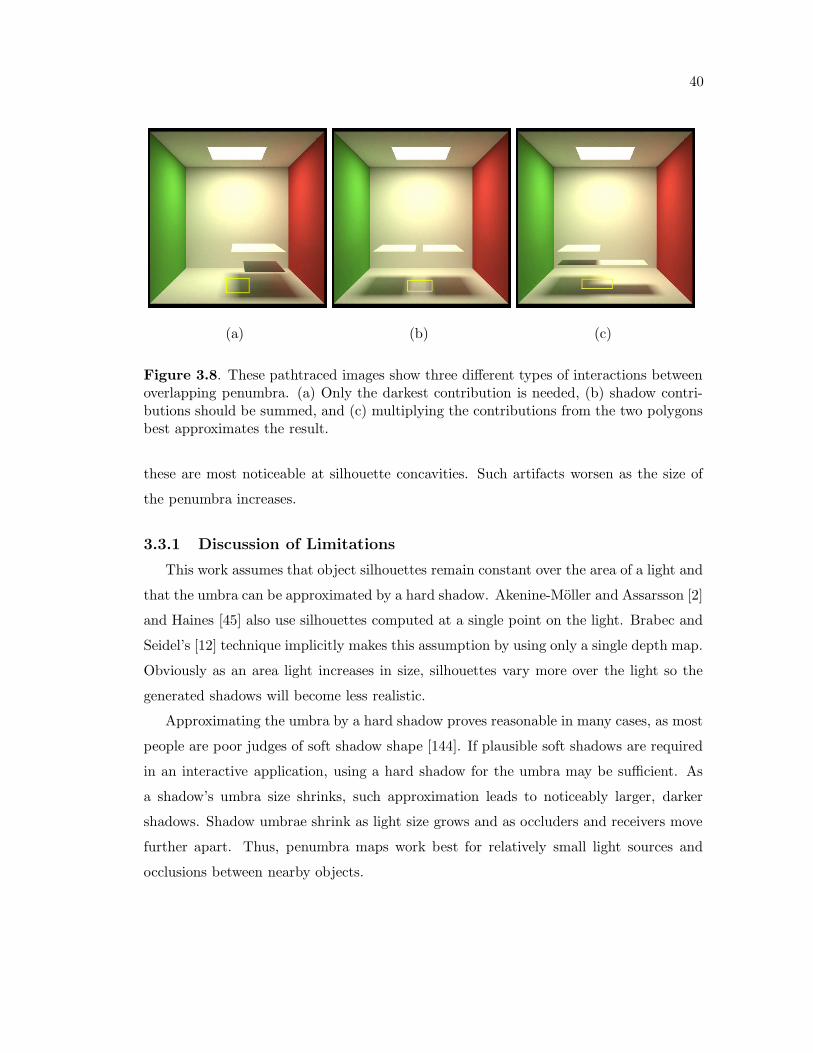
40
(a) (b) (c)
Figure 3.8. These pathtraced images show three different types of interactions betweenoverlapping penumbra. (a) Only the darkest contribution is needed, (b) shadow contri-butions should be summed, and (c) multiplying the contributions from the two polygonsbest approximates the result.
these are most noticeable at silhouette concavities. Such artifacts worsen as the size of
the penumbra increases.
3.3.1 Discussion of Limitations
This work assumes that object silhouettes remain constant over the area of a light and
that the umbra can be approximated by a hard shadow. Akenine-Moller and Assarsson [2]
and Haines [45] also use silhouettes computed at a single point on the light. Brabec and
Seidel’s [12] technique implicitly makes this assumption by using only a single depth map.
Obviously as an area light increases in size, silhouettes vary more over the light so the
generated shadows will become less realistic.
Approximating the umbra by a hard shadow proves reasonable in many cases, as most
people are poor judges of soft shadow shape [144]. If plausible soft shadows are required
in an interactive application, using a hard shadow for the umbra may be sufficient. As
a shadow’s umbra size shrinks, such approximation leads to noticeably larger, darker
shadows. Shadow umbrae shrink as light size grows and as occluders and receivers move
further apart. Thus, penumbra maps work best for relatively small light sources and
occlusions between nearby objects.

41
3.4 Results
The prototype penumbra map implementation uses OpenGL and was tested on three
systems: a 2.0 GHz Pentium 4 PC with an ATI Radeon 9700 PRO graphics card,
a 2.66 GHz Pentium 4 PC with an nVidia GeForce 5900 Ultra graphics card, and a
3.2 GHz Pentium 4 PC with a prerelease nVidia GeForce 6800 GT graphics card (with
a 300 MHz core clock speed and 500 MHz DDR memory). Vertex and fragment shaders
(see Appendix A) utilize the OpenGL ARB vertex program and ARB fragment program
extensions. Both the shadow and penumbra maps are rendered into p-buffer textures, a
type of onboard memory buffer, for direct use without necessitating a read-back through
main memory.
All scenes are rendered at 1024 x 1024 with shadow and penumbra maps of the same
size. As soft shadows effectively blur detail, simplified models of complex objects such
as the bunny, buddha, and dragon can be used to render the shadow and penumbra
maps while still retaining equivalent quality shadows. This increases aliasing artifacts,
though adding a larger bias can help reduce them. 10,000 polygon models were used to
generate shadows for the bunny and the dragon (Figures 3.9 and 3.10). Buddha’s shadow
(Figure 3.2) uses 5,000 polygons. Table 3.1 shows framerates for these models using
penumbra and shadow maps. Note that for comparison purposes, the hard shadows were
timed using a fragment program similar to the one used for penumbra maps. This program
computes the Phong lighting and performs the lookup into the shadow map, which is
significantly slower than using other capabilities of the hardware designed specifically for
those operations.
Thirty percent of the computation time is used for brute force silhouette extraction.
Thirty-five percent is spent rendering the penumbra map and the render pass consumes
the remaining time. Note that the render pass includes fragment code to perform lighting
Table 3.1. Framerate comparison between shadow and penumbra maps.Object Penumbra Shadow Penumbra Shadow Penumbra Shadow
Map on a Map on a Map on a Map on a Map on a Map on aRadeon Radeon GeForce GeForce GeForce GeForce
9700 PRO 9700 PRO 5800 Ultra 5800 Ultra 6800 GT 6800 GTBunny 18.1 42.0 19.9 30.0 67.9 97.2Dragon 14.5 48.1 15.0 30.0 44.9 108.2Buddha,
1 Light 18.1 48.1 15.0 30.0 45.3 109.3
Buddha,2 Lights 11.0 27.4 6.67 20.0 21.6 68.8

42
(a) (b)
(c) (d)
Figure 3.9. Penumbra map results for the Stanford bunny. Comparison of shadow maps(a), penumbra maps with two different sized lights (c,d), and a pathtraced shadow usingthe larger light (b). For this data set, a 10,000 polygon model is used to render theshadows onto the full (∼70,000 polygon) model.

43
(a) (b)
(c) (d)
Figure 3.10. Penumbra map results for the dragon model. Using a standard shadowmap (a) results in hard shadows (b), add a penumbra map (c) to get soft shadows (d).Using a 10,000 polygon dragon model for shadow generation and a 50,000 polygon modelto render, 1024 × 1024 images render at 44.9 fps.

44
computations and check light visibility using the shadow map. These operations take
15 of the 22 instructions in the ARB fragment program. To render penumbra maps,
the prototype application uses a fragment program with 24 assembler instructions. See
Appendix A for these shader programs.
This chapter presented the penumbra map, a new technique for rendering approximate
soft shadows in real-time. Penumbra maps allow dynamically moving polygonal models
to cast soft shadows onto themselves and other complex objects. These results work best
for relatively small penumbrae. Penumbra maps provide a simple multipass extension to
shadow mapping for easy incorporation into existing shadow map-based systems.

CHAPTER 4
INTERACTIVE RENDERING OF
CAUSTICS
Daily life immerses everyone in environments rich in illumination, particularly compli-
cated specular effects such as caustics. These effects are important to capture in computer
renderings. Unfortunately rendering complex illumination such as a caustic often incurs a
significant computational cost. Since many applications require interactive speeds, costly
path tracing algorithms for computing caustics are often infeasible, and hybrid techniques
suffer from a common computer graphics problem—poor scaling with scene complexity.
Often techniques that run quickly on simple scenes bog down when used on a complex
environment.
Although global illumination appears to have a significant impact upon how humans
view interactions between objects, computing a full global illumination solution is often
unnecessary. In fact, global illumination provides humans perceptual cues as to relative
object locations, yet accuracy is not always important [56, 71]. Some researchers [111]
have looked into simplifying the environment to reduce unnecessary computations, but
questions remain as to what level of simplification compromises the perceived quality of
global illumination.
This chapter examines the focusing of light caused by reflective and refractive surfaces.
This focusing, known as a “caustic,” potentially affects the entire environment, yet in most
cases appears in a relatively localized space around a specular object. For example, one
might see a caustic from a glass figurine on a table (see Figure 4.1) or the caustic from a
mirror on an adjacent wall.
This chapter explores a technique for sampling the caustic near a focusing object. This
allows the reduction of caustic rendering to a localized property which can be computed
with a simple lookup. This lookup can be performed at interactive framerates, even
as objects and lights move. However, sampling takes significant precomputation and
memory, and accurate caustics are limited to the sampled region.

46
(a)
(b)
Figure 4.1. A scene with caustics from a glass bunny. Using a raytracer running on 30processors, this scene (a) runs at 2.3 fps while allowing movement of either the bunny orthe light, compared to (b) 25 seconds for shooting photons for a photon mapped image.

47
The rest of this chapter is divided as follows. Section 4.1 discusses the behavior of
caustics and suggests ways to deal with their complexities. Section 4.2 discusses various
ways to sample a caustic and the tradeoffs involved and Section 4.3 discusses some issues
involved in rendering a caustic from sampled data. Section 4.4 presents the results.
Finally, Section 4.5 discusses conclusions and future work.
4.1 Caustics
This section describes the behavior of caustics and discusses assumptions and simpli-
fications used to interactively render caustics. The goal was to develop a method that
locally approximates a caustic, which requires little or no recomputation from frame to
frame even as objects and lights move.
4.1.1 Caustic Behavior
Caustics result from focused light due to reflection or refraction off specular sur-
faces [93]. Some examples of caustics in daily life include sunlight reflected off a watch
onto a car ceiling, the cardioid shape at the bottom of a coffee mug (Figure 1.7(a)), and
the focusing of light through a magnifying glass (Figure 1.7(c)).
Caustics are common, yet few people understand exactly how they should look. For
example, one would expect a glass figure to cast a caustic onto a table, but blurred,
slightly offset, or even missing details may go unnoticed.
Flat surfaces, like mirrors, reflect light without focusing it. However any concave
reflector focuses light into bright lines or points. Technically, only curved surfaces cause
caustics, but this chapter adopts the common graphics usage and refers to any specularly
reflected or refracted light as a caustic, as both planar and curved specular surfaces lead
to important illumination effects.
Consider a transmissive object fixed relative to a lightsource, as in Figure 4.2. The
caustic’s intensity at point p changes based upon the position of p relative to the object
and the normal ~Np of the surface at p. For fixed light and object positions, the caustic
can be considered a five-dimensional function. Allowing the light (or equivalently the
object O) to move changes the caustic into a eight-dimensional function, by allowing the
vector ~L to vary.
Rendering caustics interactively involves quickly evaluating this eight-dimensional
caustic intensity function. Unfortunately, analytical descriptions of an arbitrary object’s

48
~Dp
~L
~Np
O
Surface Sp
Figure 4.2. The eight dimensions of a caustic. Given the object O at point p on surfaceS, the caustic function has three dimensions from ~Dp, three dimensions from ~L, and two
dimensions from the orientation ~Np of the receiving surface relative to ~Dp.
caustic cannot be obtained using current methods, so a numerical approximation to this
function is used.
4.1.2 Simplifying the Problem
A number of simple observations allow simplification of the problem:
• The direction of incoming light often has greater impact on the visible caustic than
distance to the light.
• Lights located relatively far away generate caustics similar to those of lights located
infinitely far away.
• Most objects that focus light are relatively far away from the light. The most
prevalent exception, mirrors in light fixtures, can usually be treated as part of the
lightsource (e.g., Canned Lightsources [55]).
• The most complex caustic behavior usually occurs in regions near the focusing
object.
These observations allow some simplifying assumptions. Combining the first two obser-
vations, a directional light source can replace point lights (i.e., ignoring the distance to
the light). Using directional light sources reduces the dimensionality of the problem by

49
one.
Furthermore, limiting caustics to some finite volume around a reflective or refractive
surface allows samples to be focused in regions where the caustics contributes significantly
to the illumination of other objects. This allows sampling ~Dp over a finite region. Outside
this region, extrapolated samples from the outermost samples can approximate the caus-
tic. Alternately, outside the sampling region caustic contributions could be gradually
faded. Note that considering the caustic a local object property limits interactively
rendered caustics to diffuse surfaces, to avoid specularly reflecting the precomputed
caustic.
Finally, assuming a known surface orientation, ~Npfixed, reduces the dimensionality by
two. Incorporating this known surface orientation into the sampling allows approximation
of the caustic for an arbitrary orientation ~Np by multiplying the precomputed intensity
by ~Np · ~Npfixed. This approach was found to work for ~Npfixed
= −Dp = − ~Dp/‖ ~Dp‖ at
each sample p. Conceptually, this method treats all caustic light from O as coming from
a point light at O’s center and computes the caustic intensity at p using a cosine falloff
based on ~Np · −Dp. As discussed above, the local sampling limits rendered caustics to
mainly diffuse surfaces, so using a cosine falloff is appropriate.
Using these assumptions a simplified five-dimensional caustic function can be sampled.
These five dimensions are x, y, z, φ, and θ, where ~Dp = (x, y, z), and φ and θ correspond
to the direction of L.
4.2 Caustic Sampling
This section outlines a number of approaches for sampling and representing the five
dimensional caustic function discussed above. Since these sampled caustics are local
properties of an object, sampling must be independently performed on each object which
focuses light. Sampling of the volume over x, y, and z is discussed separately from the
sampling of incoming light directions φ and θ.
4.2.1 Sampling the Light
For each caustic object, information about how the caustic changes as the light moves
must be stored. Due to the assumption of directional lighting, sampling varying light
positions is equivalent to sampling directions (φ, θ) over a unit sphere. Each such sample
(φi, θi) is referred to as a light sample Li.

50
Sampling φ and θ in a fixed, uniform or near-uniform, pattern generally works as
well as adaptively sampling. Each linear change in φ or θ corresponds to varying non-
linear changes (see Figure 4.3) in the caustic intensity over the volume (x, y, z). Because
incoming light often bounces around the object many times, few incoming directions L
have a “simpler” caustic behavior than others. Thus, adaptive sampling of the sphere
tends to quickly converge to a relatively uniform sampling.
The rest of this chapter uses φ and θ sampled on a geodesic. Specifically, we subdivide
an icosahedron between three and six times and project the vertices to the unit sphere.
Samples can be taken as either the vertices or centers of the subdivided triangles. This
provides a nearly uniform sampling over the sphere, but has the advantage that existing
samples need not be recomputed for denser samplings (i.e., subdivisions) of the sphere.
4.2.2 Sampling Space
For each light sample Li, some region around object O should be sampled. If the
object has a bounding volume of radius r, tests showed a region with radius ≈ 3r should
be sampled to capture the most important regions of the caustic. However, this varies
depending on where focal points of the object lie.
Two different approaches to storing volumetric samples were examined, a uniform grid
and a set of concentric shells subdivided as a geodesic (see Figure 4.4). After selecting a
representation for the volume, sampling the caustic function uses the following algorithm.
For each light sample Li, we shoot photons from the directional lightsource towards the
object O. Once a photon specularly bounces, it contributes to all the cells it passes
though (the dashed lines in Figure 4.4).
Figure 4.3. Popping between adjacent light samples. Here a minute change in objectposition results in a nonlinear change to the caustic, as a different light sample is usedafter movement.

51
LiLi
Figure 4.4. Sampling space on either a uniform grid or a set of concentric shells.
A photon’s contribution to a cell is computed as if it hit a surface at the sample
point ps with surface normal in the direction of Ocenter − ps. Each sample point ps
stores only the caustic intensity (i.e., no direct lighting is included), so contributions
from nonreflected and nonrefracted photons are ignored. The result is a grid storing
approximate irradiance at each cell’s center (similar to the Irradiance Volume [44]), with
the caveat that only irradiance due to specularly reflected light is stored.
Storing data on a grid has the advantage of easy implementation and fast lookups.
However, a rectangular grid structure does not correspond well to caustic data because
intensity data changes in a generally radial fashion. This means much space is wasted
storing data which changes slowly and not enough is concentrated in regions where the
caustic changes quickly.
Storing data on concentric shells allows nonuniform placement of the shells to densely
sample the data radially in regions where the caustic varies significantly. Using this allows
a reduction of the sampling frequency in one dimension by up to a factor of five, either
reducing memory usage or allowing a finer sampling in other dimensions. To avoid the
difficulty of indexing into a geodesic, a table lookup is used.
4.2.3 Data Representation
One of the major problems with sampling a high dimensional function, such as
the caustic intensity, is the large storage requirement. Using such data in interactive
applications can be difficult if significant portions must remain in memory. A number of
methods to represent these data can reduce the memory overhead. Each approach has

52
its advantages and disadvantages.
A naive implementation stores a complete set of sampled data, both on disk and in
memory. Obviously, this requires a machine with lots of memory. For instance, storing all
sampled data for the ring images (see Figure 4.5) requires around a gigabyte of memory,
with data stored in colors of three bytes each: one byte for each the red, green, and
blue channels. The advantage of this technique is easy implementation and fast lookups,
leading to faster framerates when the data completely resides in main memory. Since
caustics typically have a large dynamic range, we cannot use these bytes to store the
usual values in the range [0, 1]. The examples shown require intensity values in the [0, 3]
(a) (b) (c)
(d) (e) (f)
Figure 4.5. Sharper caustics come at the expense of denser sampling. The images shownrequire (a) 5.7, (b) 22.5, (c) 90.1, (d) 360, and (e) 1440 kilobytes of memory per lightsample. The data is stored using the concentric shell representation. Compare to (f) aphoton traced solution. Using a multiresolution approach, similar results require (a) 4.8,(b) 12.6, (c) 29.5, (d) 70.4, and (e) 179 kilobytes of memory per light sample.

53
range. Using 8-bit values in this way obviously reduces precision; however, when using
interpolation to get the irradiance at each point, no significant degradation in quality was
noticed.
A multiresolution approach helps save memory. Multiresolution techniques that adap-
tively subdivide the sampled geodesic as needed often reduce memory usage by up to a
factor of 10 with equivalent quality results. The tradeoff is that lookups take longer due
to the more expensive data traversal routines, leading to moderately reduced framerates.
Additionally, multiresolution approaches may not always reduce storage space.
Using spherical harmonics coefficients (see Appendix B) to represent sampled data
also allows significant compression. For each cell in the volume, instead of storing a
color for each light sample Li, spherical harmonic coefficients approximating the transfer
function from the environmental luminaire to a sample point are stored. Alternately,
each set of spherical harmonic coefficients can represent the transfer from a light sample
to a single concentric shell, though rendering using the first approach is faster and more
straightforward.
One main advantage of spherical harmonics is that a large amount of data can be
approximated by a few coefficients. The major problem with the representation, however,
is that spherical harmonics eliminate most of the high frequency information in a caustic.
Such sharp features are believed to be very important for rendering caustics. Higher
order spherical harmonics better represent sharp features, but increasing the order of the
spherical harmonic approximation increases precomputation, significantly increases the
number of coefficients required, and decreases rendering speed.
4.3 Caustic Rendering
After sampling the five-dimensional caustic function, a number of approaches can be
used to render the caustic. Results in this chapter use an interactive raytracer to render
the scene, because it runs interactively on a large shared-memory machine, easily allowing
access to large amounts of memory necessary for complicated caustics. Any renderer that
can access the necessary data quickly and perform per-pixel operations could use these
sampled data to compute caustic intensity.
4.3.1 Rendering Algorithm
Raytracing the scene proceeds normally until the determination of the color at a diffuse
surface. At these surfaces, instead of just looking for direct illumination, the raytracer

54
performs lookups into the sampled data to determine if they are illuminated by a caustic.
This process can be described algorithmically as follows:
1. Determine the direction L from the center of the object O to the light. Locate the
nearest light sample Li (where L · Li is maximal). This volume stores the closest
approximation to the caustic from the current light position. This step should be
done only once per frame, since it is independent of the intersection point p.
2. At each intersection point p, find p’s location in the volume sampled around O and
look up the caustic contribution. Add this result to the direct lighting computed
by the renderer.
4.3.2 Issues Rendering Caustic Data
Unfortunately, using a single light sample Li to render the caustic causes temporal
coherence issues as objects move. This is due to differences in the caustic from one light
sample to the next (see Figure 4.3). The popping can be reduced by combining the caustic
from multiple light samples Li, Lj, and Lk (where L · Li ≥ L · Lj ≥ L · Lk ≥ L · Lm,∀m /∈i, j, k). Li, Lj, and Lk form the three vertices of a spherical triangle on the unit sphere
which includes L (see Figure 4.6).
Combining three light samples using barycentric coordinates [15] eliminates pop-
ping between caustic samples but introduces a new problem—ghosting (see Figure 4.7).
Ghosting happens because object O’s caustic can differ significantly between neighboring
light samples, so blending data from Li, Lj , and Lk results in three separate faint caustics.
Unfortunately, the best way to eliminate ghosting is to sample the caustic for more light
directions. This significantly increases memory consumption.
Below, an approach which helps reduce ghosting for relatively smooth objects is
described. This algorithm replaces step 2 from the rendering algorithm above:
A. Compute the vector ~Dp from Ocenter to p.
B. Find the barycentric coordinates of L in the spherical triangle formed by Li, Lj ,
and Lk. This gives the relative contributions from each light sample (Figure 4.6).
C. Compute the angles βi, βj , and βk between L and the three nearest sampled light
directions Li, Lj, and Lk.

55
βk
Light
Li
βi
βj
Lj
O
LkL
Figure 4.6. L intersects the spherical triangle formed by Li, Lj, and Lk.
(a) (b) (c)
Figure 4.7. Ghosting happens when the caustic changes significantly between neighbor-ing light samples Li, Lj , and Lk. Images (a) without caustics, (b) with ghost caustics,and (c) a correct caustic.

56
D. Calculate rotation axes ~Ri, ~Rj , and ~Rk by taking the cross product between ~L and
~Li, ~Lj, and ~Lk, respectively.
E. Rotate vector ~Dp around the axis ~Ri by angle βi to find a new vector ~Dp′i. Similarly
find ~Dp′jand ~Dp′
kby rotating around ~Rj and ~Rk by angles βj and βk (Figure 4.8).
F. Find the points p′i, p′
j, and p′k. Where p′
i = Ocenter + ~Dp′i.
G. Perform caustic lookups as if p′i, p′
j , and p′k were the intersection points (instead of
p). Weight the contributions from these points based on the barycentric coordinates
computed in step B.
The process performs an interpolation between samples. Unfortunately, such an
interpolation is not generally valid, as it assumes the caustic changes linearly in space
for a linear change in light direction. For relatively smooth objects, like the sphere and
bunny, such “interpolation” generally allows us to use fewer light samples. For objects
such as the cube and prism that have sharp angles, this approach does not significantly
reduce ghosting, so a large number of light samples are still required.
When using spherical harmonic coefficients, which essentially filter over the sampled
light directions, this complicated rendering process can be avoided. Instead the caustic
is computed by integrating the transfer function (stored at the samples as spherical
harmonic coefficients) with the incident illumination, as described by Green [43], Sloan
Sampled
p
LLi
Light
Light
~Dpp′
βi
~Dp′
i
Figure 4.8. Alternative approach to caustic lookups. Find the cell to use in the weightedaverage by rotating ~Dp around the axis ~Ri (which points into the page at Ocenter) by angleβi.

57
et al. [120], and Appendix B. Caustics rendered with spherical harmonics, however, tend
to be very blurry.
4.4 Results
This approach was implemented on an interactive parallel raytracer running on an
SGI Origin 3800 with thirty-two 400 MHz R12000 processors, a shared memory machine
that easily holds the entire scene and caustic datasets in main memory. However, this
approach is not limited to such applications. Any renderer that has per-pixel lighting
control could implement the technique given enough memory. Existing systems (e.g.,
[42, 96, 133, 142, 138]) could easily incorporate such precomputed caustics to avoid the
cost of reshooting photons each frame.
Table 4.1 contains timings for the images generated for Figures 4.1, 4.9, 4.10, and 4.11.
The lookups into the precomputed caustic data incur a 10–45% speed penalty when
displaying caustics, depending on the relative costs of the lookups to the raytracing costs
of the scene. The cost of the photon shooting preprocess ranges from 1.3 to 25 seconds
per light sample, using a single 400 MHz R12000 CPU. Shooting photons for a photon
map takes a similar amount of time, though additional overhead is needed to create the
required kd-tree. Framerates are reported for a 360 × 360 window running on thirty
400 MHz R12000 processors.
Figures 4.9 and 4.10 compare a photon map with precomputed caustics using both
the grid and concentric shell storage techniques. These comparisons show grids and shells
requiring roughly the same amount of memory. The figures also show data compressed
using 5th and 15th order spherical harmonics. Using the spherical harmonic represen-
tation provides advantages such as the ability to use area lights (see Figure 4.12), high
Table 4.1. Caustic rendering and precomputation times.Object Grid Shell MultiRes No 5th Order Shoot Photons
Caustics Caustics Caustics Caustics Spherical (per sample)(fps) (fps) (fps) (fps) Harmonics (sec)
(fps)Sphere 15.2 17.3 15.0 26.9 8.1 1.7Cube 12.1 12.6 10.8 20.2 6.1 2.4Prism 12.7 13.2 11.0 20.3 6.5 2.0Ring 9.3 9.5 8.8 12.9 5.2 1.3Building 1.94 2.01 1.90 2.29 1.48 4.5Bunny 2.16 2.30 2.25 2.55 1.80 25.0

58
(a) (b) (c)
(d) (e)
Figure 4.9. Caustic rendering techniques on a metal ring and glass cube. Caustics from(a) a photon map, (b) the concentric shell approach, (c) the grid technique, (d) 5th orderspherical harmonics, and (e) 15th order spherical harmonics.

59
(a) (b) (c)
(d) (e)
Figure 4.10. Caustic rendering techniques on a glass prism. Caustics from (a) a photonmap, (b) the concentric shell approach, (c) the grid technique, (d) 5th order sphericalharmonics, and (e) 15th order spherical harmonics.

60
Figure 4.11. Casting caustics on complex objects. This “building” can dynamicallycast caustics on surrounding terrain based on the sun’s position.
Figure 4.12. The caustic of a prism in St. Peter’s cathedral using 5th order sphericalharmonics. Note there are no shadows in this image.

61
temporal coherence, and low memory consumption. For comparison, these fifth order
representations use around 10 MB memory, about as much as the uncompressed data
used for Figure 4.5(a). Since the number of coefficients increases quadratically with
order, computation costs quickly become the bottleneck. All of these scenes run at less
than one frame per second using fifteenth order spherical harmonics.
Figure 4.5 illustrates the effect of sampling density on memory consumption and
caustic quality. For a relatively smooth object few light samples are necessary. The
bunny (see Figure 4.1) needed only 162 light samples. For objects where the rotational
alignment technique from Section 4.3.2 does not work well (like the cube and prism), up
to 2500 light samples are necessary. Note that number of light samples does not affect
framerate, assuming the data all fit into memory.
Obviously, with symmetric objects one need not sample the entire sphere of incoming
light directions. For a sphere, a single light sample suffices. For the metallic ring, between
50 and 100 light samples are sufficient for good temporal coherence. Many common
objects have symmetrical properties that could be used to simplify sampling.
4.5 Discussion
This chapter presented a novel technique for rendering approximate caustics inter-
actively by localizing the problem to the vicinity of the focusing object. This approach
avoids the recurring cost of photon shooting that other methods require to generate
dynamic caustics. Because particle tracing is not necessary between frames, this tech-
nique can be applied to other interactive systems that cannot traditionally perform such
computations (e.g., hardware based renderers). Additionally, the rendering costs of this
method are independent of object complexity. Since caustics are rendered using table
lookups, memory becomes the bottleneck, so a number of ways to sample, represent, and
compress the data in memory were examined.
Storing a highly sampled caustic function in memory produced the best looking results.
Unfortunately, the memory requirements make the technique difficult to use unless object
symmetries or other simplifying conditions exist. Multiresolution approaches can signif-
icantly reduce memory overhead by storing densely sampled data only where necessary.
In exchange lookups become more costly.
Spherical harmonic basis functions generally blur caustics extensively, and the results
look unconvincing. However, memory requirements are modest enough to allow imple-
62
mentation on current graphics hardware. Higher order approximations improve results at
the expense of additional coefficients, though this additional expense can quickly expand
memory requirements beyond reach of graphics hardware.
Scenes that lend themselves well to this technique include outdoor scenes where the sun
effectively acts as a constant directional lightsource. Such a scene requires a single light
sample. Leveraging object symmetries also can reduce some of the memory burden. Many
common objects have such symmetries, so these sampling techniques may be feasible for
such objects.
This work has a number of limitations, including extensive memory requirements for
general environments requiring the entire sampled space, poor realightment of neighboring
samples, and inability to handle area lights without spherical harmonics. However, by
tailoring the caustic representation to the application, these limitations can be overcome.
Thus, the results presented in this chapter indicate that viable techniques exist for
including specular effects as well as diffuse global illumination in interactive applications.

CHAPTER 5
INTERACTIVE RENDERING OF
ISOSURFACES WITH GLOBAL
ILLUMINATION
Isosurfaces, also known as implicit surfaces or level sets, are widely used in computer
graphics and scientific visualization, whether to help model complex objects [112] or to re-
veal the structure of scalar-valued functions and medical imaging data [69]. Because both
computational and acquired datasets tend to be large, only recently has interactive display
and manipulation of surfaces with varying isovalues become feasible for full-resolution
datasets [97]. In most interactive visualization systems, the rendering of isosurfaces is
based on only local illumination models, such as Phong shading, perhaps coupled with
simple shadows. For partially lit concave regions, these simple shading models fail to
capture the subtle effects of interreflecting light and shadows. These regions are typically
dominated by a local ambient term which provides no cues to environmental visibility or
reflections from nearby surfaces. Figure 5.1 shows the details brought out by the approach
introduced in this chapter, both in shadowed regions and those with high interreflections.
One usually thinks of “direct lighting” as coming from a small light source, but it can
also come from extended light sources. In the extreme case the entire sphere of directions
is a light source and “shadowing” occurs when not all of the background is visible at a
point. This results in darkening for concavities, exploited as accessibility shading [87] and
obscurance shading [155]. More recently, direct lighting from a uniform extended source
has been applied to illuminating isosurfaces extracted from volumes to good effect [131].
This chapter extends the class of lighting effects for isosurfaces to include full global
illumination from arbitrary light sources. The new method requires an expensive pre-
process but does not greatly affect interactive performance, and can even speed it up
since shadows can be precomputed and stored. This approach uses a conventional
three-dimensional texture to encode volume illumination data. For static illumination
and a static volume, a scalar texture encoding irradiance stores the necessary global

64
(a) (b)
(c) (d)
Figure 5.1. Comparison of (a,c) globally illuminated and (b,d) Phong shaded isosurfaces.Note the improvement in regions dominated by indirect lighting, particularly in the eyesockets (a,b) and the concavities in the simulation data (c,d).

65
illumination for all isosurfaces. For dynamic lights and complex materials, multiple values
are used per texel, as in Sloan et al. [120]. In either case, rendering interpolates between
neighboring texels to approximate the global illumination on the correct isosurface.
The next section introduces some volume rendering terminology and describes the
illumination models for display. Section 5.2 gives an overview of the new illumination
technique, and Section 5.3 describes the algorithm in greater detail. Section 5.4 discusses
the results.
5.1 Background
Rendering images of isosurfaces can be accomplished by first extracting some surface
representation from the underlying data followed by some method of shading the iso-
surface. Alternatively, visualizing isosurfaces with direct volume rendering requires an
appropriate transfer function and a shading model.
In practice, many volume datasets are rectilinearly sampled on a three-dimensional
lattice, and can be represented as a function ρ defined at lattice points xi. Some
interpolation method defines ρ(x) for other points x not on the lattice. Other datasets
are sampled on a tetrahedral lattice with an associated interpolation function. Analytical
definitions are also possible for ρ(x), often arising out of mathematical applications. Such
analytical representations can easily be sampled on either a rectilinear or tetrahedral
lattice.
Given a sampled dataset ρ(xi), the marching cubes algorithm [79] extracts explicit
polygons approximating an isosurface I(ρiso) with isovalue ρiso, where I(ρiso) = x | ρ(x) =
ρiso. Various improvements make this technique faster and more robust, but these
improvements still generate explicit polygonal representations of the surface. Raytracing
and volume rendering provide an alternate method of displaying isosurfaces, which need
not construct and store a polygonal representation [76, 97]. Once an isosurface has been
identified, standard illumination models can be applied to help visualize the data.
Commonly, extracted isosurfaces are shaded using the Phong model [102] and vari-
ations using similar ambient, diffuse, and specular components. Such techniques give
poor depth and proximity cues, as they rely on purely local information. Illumination
techniques for direct volume rendering, such as those surveyed in Max [84], allow translu-
cency and scattering along the viewing ray and shadow rays, but they fail to allow area
lights and are not interactive. Sobierajski and Kaufman [124] apply global illumination
66
to volume datasets, but they shade at runtime, so few effects can be incorporated while
maintaining interactivity.
Several techniques have been proposed to interactively shade volumes with global
lighting. The Irradiance Volume [44] samples the irradiance contribution from a scene,
allowing objects moving around the scene to be shaded by static environment illumination.
However, objects placed in the Irradiance Volume cannot interact with themselves, which
is important for correct global illumination of isosurfaces. Precomputed radiance transfer
techniques [90, 119, 120] can be used to shadow or cast caustics on nearby objects
by sampling transfer functions in a volume around the occluder. Unfortunately, these
techniques do not allow dynamic changes to object geometry, which is important when
exploring the isosurfaces of volume datasets. Kniss et al. [73] describe an interactive
volume illumination model that captures shadowing and forward scattering through
translucent materials. However, this method does not allow for arbitrary interreflec-
tions and thus does not greatly improve isosurface visualization. The vicinity shading
technique of Stewart [131] encodes direct illumination from a large uniform light in a
three-dimensional texture and allows its addition to standard local shading models while
interactively changing the displayed surface. However, this method provides an approach
for only direct illumination and does not incorporate indirect illumination.
5.2 Overview
A brute-force approach to globally illuminating an isosurface would compute illumina-
tion at every point visible from the eye. Figure 5.2 shows how a Monte Carlo path tracing
technique would perform this computation. Obviously, performing such computations on
a per-pixel basis quickly becomes cost prohibitive, so caching techniques [146] are usually
preferable. Many existing techniques cache radiance [10], irradiance [44], or more complex
transfer functions [90, 106, 120] to speed illumination computations.
In volume visualization, users commonly change the displayed isovalue, thereby chang-
ing the isosurface, to view different structures in the volume. Most illumination caching
techniques are object specific, so as the surface changes new illumination samples must
be computed. This chapter introduces a technique that stores either irradiance or more
complex transfer functions in a three-dimensional texture coupled with the volume. Each
texel t corresponds to some point xt in the volume. The process is broken into two
steps. During the computation step, illumination values can be computed using any

67
Light
pisosurface
~n
Figure 5.2. Computing the irradiance at point p involves sending a shadow ray andmultiple reflection rays. Reflection rays either hit the background or another part of theisosurface, in which case rays are recursively generated.
standard global illumination technique. For each texel t, extract the isosurface I(ρ(xt))
running through xt. Using this isosurface, compute the global illumination at point
xt via standard approaches and store the result in texel t. Figure 5.3 shows how this
works for four adjacent samples using a Monte Carlo sampling scheme. When rendering,
interpolate between cached texels to the correct isosurface, allowing for interactive display
of arbitrary isosurfaces.
As with most illumination caching techniques, the rationale behind this approach is
that global illumination generally changes slowly for varying spatial location. Here this
assumption applies in two ways: illumination should change gradually over a surface and
illumination should change gradually with changing isosurfaces.
One situation exists where this approximation obviously breaks down—hard shadows.
Hard shadows involve a very visible discontinuity in the direct illumination. As shown in
Figure 5.3, each sample in the illumination lattice is potentially computed on a different
isosurface. In regions where a shadow discontinuity exists, some samples will be in shadow
and others will be illuminated. Using an interpolation scheme to compute the illumination

68
Figure 5.3. The global illumination at each texel t is computed using standard techniquesbased on the isosurface I(ρ(xt)) through the sample.
results in a partially shadowed point between samples. Thus for a static isosurface, results
near shadow edges will be blurred, similar to the effect achieved with percentage closer
filtering [109].
Since dynamically changing the rendered isosurface is desirable, the effect of such
changes on shadow boundaries must also be considered. As the displayed isosurface
changes, the interpolated illumination value on the surface changes with distance from
illumination samples, just as the illumination varies over a single isosurface. Thus, faint
shadows may exist when there is no apparent occluder or small occluders may cast no
shadow. The effect is that shadows will “fade” in and out as occluders appear and
disappear. Examples of these effects can be seen in Figure 5.4. The scene is illuminated

69
Figure 5.4. The Visible Female’s skull globally illuminated using the new technique.The right images show how the cord’s shadow fades out with increasing isovalues.
by a blue and brown environment with a yellow point light source. The shadows are
blurred slightly, and as the isosurface changes the cord fades out before its shadow.
Note that because sharp discontinuities in direct illumination are most visible, hard
shadow are a worst-case scenario. For soft shadows or indirect illumination the perceived
effects are less pronounced, so this approximation of a smoothly changing illumination
function becomes more accurate. Artifacts similar to those in Figure 5.4 may still occur,
but they will be less noticeable.
The artifacts that occur with changing isovalues arise from approximating the non-
linear global illumination function using simple trilinear interpolation. This approxima-

70
tion is what causes the “fading” of shadows and the faint banding seen in the results.
This assumption occasionally causes problems, but the proposed technique provides
significantly more locality information than local models, especially in concavities and
dark shadows where ambient terms either provide little or conflicting information. Ad-
ditionally, since shadows are included in the representation, they require no additional
computation. In fact, this technique renders faster than simple Phong and Lambertian
models when including hard shadows.
5.3 Algorithm
This technique has two stages: illumination computation and interactive rendering. A
simplistic approach would perform all the computations as a preprocess before rendering.
As this can require significant time and not all illumination data may be required, it
is possible to lazily perform computations as needed, assuming the display of some
uncomputed illumination is acceptable until computations are complete.
5.3.1 Illumination Computation
Each sample in the illumination lattice stores some representation of the global illu-
mination at that point. This illumination is described by the rendering equation (from
Section 1.2.3), without the emission term:
L(xt, ~ωout) =
∫
Ωfr(xt, ~ωout, ~ωin)L(xt, ~ωin) cos θind~ωin,
where xt is the location of the illumination texel t with normal ~nt, ~ωout is the exitant
direction, ~ωin is the incident direction varying over the hemisphere Ω, and fr is the BRDF.
Note that cos θin is equivalent to ~ωin · ~nt, which is used in the rest of this chapter.
Depending on an application’s required materials and illumination this equation and
the representation stored in the illumination texture can be varied to reduce computation
time and storage space. For a simple diffuse surface with fixed lighting, a single irradiance
value is sufficient at each lattice point. In this case, the rendering equation can be
rewritten as:
L(xt) = fr(xt)
∫
ΩL(xt, ~ωin)(~ωin · ~nt)d~ωin =
R(xt)E(xt)
π. (5.1)
Here the diffuse BRDF has no dependency on ~ωin. It can be removed from the integral
and is then equivalent to the surface albedo R(xt) divided by π. The remainder of the

71
integral is the irradiance at point xt, E(xt). Storing E(xt) in a texture allows for easy
illumination during rendering, as per Equation 5.1.
The simplest way to compute the irradiance at each sample point xt uses naive Monte
Carlo pathtracing. Using N random vectors, ~vj, sampled over the hemisphere Ω, the
irradiance is approximated:
E(xt) =1
N
N∑
j=1
L(xt, ~vj). (5.2)
Using this equation, compute the irradiance at every point as shown in Figure 5.5.
Explicitly extracting different isosurfaces for each sample is quite costly. To avoid this
cost, a raytracer performs intersections with the trilinear surface analytically [98]. Unfor-
tunately, trilinear techniques generate noisy surfaces and normals, which can significantly
impact the quality of the computed global illumination (see Figure 5.6). Rather than
directly computing normals from the analytical trilinear surface or using a simple finite
difference gradient, a smoothed normal defined by a tricubic B-spline kernel applied to the
gradient over a 4×4×4 voxel region gives better results. Smoothing normals and slightly
offsetting xt in the normal direction during illumination computations significantly re-
duces this microscopic self-shadowing noise. Note the global illumination artifacts seen
in Figure 5.6 using gradient normals occur on both microscopic and macroscopic scales.
Noise occurs on the microscopic scale due to aliasing on the trilinear surface. Artifacts
occur on the macroscopic scale when the volumetric dataset and the illumination volume
have different resolutions. Visible bands occur where voxels from the two volumes align,
as can be seen in Figure 5.6(d).
For more complex effects such as dynamic illumination or nondiffuse material BRDFs,
a simple irradiance value will not suffice, and a more complex representation of the
for all xt in illumination lattice do
compute isovalue ρ(xt)compute isosurface normal ~nt
sample hemisphere Ω defined by ~nt
for all samples ~vi ∈ Ω do
compute illumination at xt in direction ~vi using isosurface with isovalue ρ(xt)end for
compute irradiance at xt using equation 5.2.end for
Figure 5.5. Pseudocode to compute irradiance at samples in the illumination lattice.

72
(a) (b) (c)
(d) (e)
Figure 5.6. An isosurface from the Visible Female’s head extracted using analyticalintersection of the trilinear surface. Direct illumination from a point light using (a)gradient normals, (b) tricubic B-spline smoothed normals, and (c) offset surface withsmoothed normals. Four bounce global illumination using (d) gradient normals and (e)offset surface with smoothed normals.

73
illumination must be computed. Choosing to use spherical harmonic (SH) basis functions
to store more complex illumination efficiently represents low frequency lighting. As
diffuse global illumination tends to vary smoothly over space, such a representation makes
sense. Spherical harmonics allow for dynamically changing illumination as well as quick
integration during rendering, using a simple dot product or matrix multiply operation.
Assuming a diffuse material, incident illumination from a distant environment L∞(~ωin)
invariant over x, and a visibility function V (xt, ~ωin), the rendering equation can be
rewritten as:
L(xt) = fr(xt)
∫
Ω
[
L∞(~ωin)V (xt, ~ωin)(~ωin · ~nt) + L(x~ωint )(1 − V (xt, ~ωin))
]
d~ωin. (5.3)
Note x~ωint is the point occluding xt in direction ~ωin. As the incident illumination is
assumed constant over the volume, it can be factored out of the recursive integrals
when using the SH basis, leaving a geometry term whose coefficients can be computed
numerically using Monte Carlo techniques. Green [43] clearly explains this process in
great detail. Every point in the illumination texture stores SH coefficients of this geometry
term.
Similar SH values can be computed and stored at voxels for more complex materials
including glossy or transparent effects, as described in Sloan et al. [120, 119]. Additionally
other bases, like wavelets, could be used to represent the global illumination in the volume,
especially if higher frequency effects are desired.
5.3.2 Interactive Rendering
After computing the illumination samples, rendering is straightforward. At every
visible point on the displayed isosurface, first index into the illumination texture to find
the eight nearest neighbors. Afterwards, interpolate the coefficients stored in the texture,
and use the interpolated coefficients for rendering.
When using an irradiance texture, simply use Equation 5.1 to compute the illumina-
tion based on the stored irradiance and the albedo. With the spherical harmonic repre-
sentation, interpolate the stored spherical harmonic geometry coefficients and perform a
vector dot product with the environmental lighting coefficients.
A higher order interpolation [83] scheme over nearby neighbors was expected to gen-
erate better smooth illumination over complex isosurfaces. Interestingly, simple trilinear
interpolation of stored coefficients proved sufficient. More complex interpolation schemes
gave equivalent or even worse results, as shown in Figure 5.7. Methods with larger kernels

74
(a) (b)
(c) (d)
Figure 5.7. Approaches to interpolating between illumination samples. Engine blockilluminated using (a) the illumination sample with closest isovalue, (b) the nearestillumination sample, (c) a trilinearly interpolated value, or (d) a value computed with atricubic B-Spline kernel.
generally gave worse results due to the increased likelihood of interpolating samples from
widely different isosurfaces.
5.4 Results
Several different approaches were used to implement this technique. First, a Monte
Carlo pathtracer computed the illumination at texels throughout the volume. Utilizing
the precomputations in an interactive raytracer allows dynamic changes to the visualized
surface and illumination. An extension to the interactive raytracer allowed computation
of illumination lazily, avoiding computations for isosurfaces never seen. Finally, import-
ing the illumination texture into an OpenGL visualization program allows interactive

75
rendering of global illumination on a single PC.
The interactive raytracer runs in parallel on an SGI Origin 3800 with sixty-four
600 MHz R14000 processors. This is a shared memory machine with 32 GB of memory,
allowing for easy access to large volume datasets and illumination textures. Large SGIs
are uncommon, but users generating and interactively displaying large volume datasets
typically have access to similarly powerful machines (or clusters [27]) which could apply
this technique. The OpenGL implementation runs on a Dell Precision 450 with 1 GB
memory and an Intel Xeon at 2.66 GHz. The graphics card is a GeForce FX 5900 with
256 MB memory. The code utilizes only simple fragment shaders, so older cards should
suffice, but the increased graphics card memory facilitates visualizing bigger volumes.
Computing global illumination values for every texel in a volume can be quite ex-
pensive, whether computing simple irradiances or sets of spherical harmonic coefficients.
Table 5.1 shows illumination computation timings for the volume shown in Figure 5.8.
Times are shown for computing the entire texture as well as for the single views shown
in Figure 5.8. The prototype uses naive, unoptimized Monte Carlo pathtracing, on
thirty 400 MHz R12000 CPUs, for precomputation. More intelligent algorithms would
significantly reduce these precomputation times.
For volumes with few interesting surfaces such as the engine block, computing illu-
mination on the fly may be preferential to a long precomputation, as global illumination
samples reside near displayed isosurfaces. Samples elsewhere can remain uncomputed. At
a 512× 512 resolution, computing a single irradiance for each sample takes a few seconds
per viewpoint using sixty 600 MHz R14000 CPUs. Densely sampled illumination textures
and complex environmental lighting require longer computations, as shown in Table 5.1.
In either case lazy computation maintains interactivity, so viewpoint and isovalue can be
changed during computation.
Table 5.1. Illumination computation timings for images from Figure 5.8.100 625 2500 10000
Sample type samples samples samples samplesper voxel per voxel per voxel per voxel
Spherical harmonics (single image) 0.33 min 2.63 min 10.6 min 48.2 minSpherical harmonics (full texture) 8.47 min 52.8 min 210 min 853 minIrradiance samples (single image) 0.95 min 5.80 min 23.7 min 98.3 minIrradiance samples (full texture) 18.2 min 113 min 450 min 1806 minPathtraced (single image) 0.73 min 4.51 min 18.0 min 72.1 min
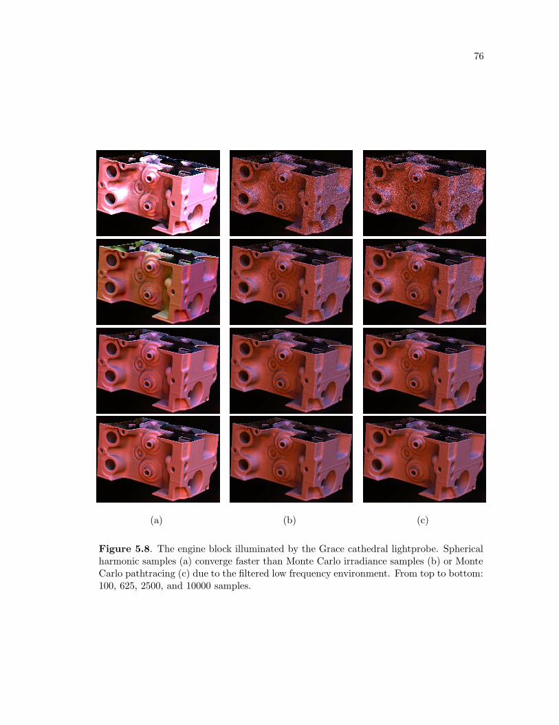
76
(a) (b) (c)
Figure 5.8. The engine block illuminated by the Grace cathedral lightprobe. Sphericalharmonic samples (a) converge faster than Monte Carlo irradiance samples (b) or MonteCarlo pathtracing (c) due to the filtered low frequency environment. From top to bottom:100, 625, 2500, and 10000 samples.

77
Precomputation is slow, but it need be done only once. Using the resulting illumi-
nation is simple and quicker than most lighting models used for visualization. Table 5.2
compares framerates using Phong and Lambertian materials with this technique. Timings
use the interactive raytraced implementation on either thirty or sixty 600 MHz R14000
CPUs with image resolutions of 512 × 512. Notice that rendering from either spherical
harmonic coefficients or a single irradiance sample is faster than simple shading with hard
shadows. Yet both these techniques include shadows along with other global illumination
effects.
Table 5.2 also shows the memory overhead for this technique. The irradiance sample
requires one RGB triplet per voxel, stored as one byte per color channel. Using the same
resolution as the volume dataset requires as much as three times more memory as simply
storing the volumetric data. The spherical harmonic representation uses no compression,
so a fifth order representation uses 25 floating-point coefficients per channel, or two orders
of magnitude more memory. Using compression techniques from Sloan et al. [119] would
help reduce memory usage.
Simulation data, like the Richtmyer-Meshkov instability dataset shown in Figures 5.9,
5.10, and 5.11, also benefits from global illumination. Often such data are confusing so
shadows and diffuse interreflections can give a sense of scale and depth lacking in Phong
and Lambertian renderings. Figures 5.9, 5.10, and 5.11 compare the new technique
to vicinity shading, Phong, and Lambertian with and without shadows. The Phong
and Lambertian images use a varying ambient component based on the surface normal.
Figures 5.10 and 5.11 also compare with a local approach that adds distance information
using OpenGL-style fog.
Vicinity shading provides better results than Phong or Lambertian models, but in-
cident illumination must be constant over the environment, such as on a cloudy day.
Vicinity shading turns out to be a special case of a full global illumination solution. By
Table 5.2. Comparison of framerates and memory consumption for Figure 5.8.Material Type Frames per second Frames per second Extra memory used
(on 30 CPUs) (on 60 CPUs) (in MB)Diffuse, No Shadows 17.0 33.1 0
Diffuse, With Shadows 8.75 17.3 0Phong, With Shadows 8.60 17.0 0
Irradiance Samples 15.6 30.5 9.75Spherical Harmonics 11.7 21.7 975

78
(a)
(b)
(c)
Figure 5.9. An enlarged portion of the Richtmyer-Meshkov dataset shown in Figure 5.11.These images enlarge a crevice in the upper right corner of images from the right columnusing (a) the new approach, (b) vicinity shading, and (c) Phong with varying ambientcomponent.

79
(a) (b)
(c) (d)
(e) (f)
Figure 5.10. A Richtmyer-Meshkov instability simulation under various illumination.A view using (a) the new technique, (b) vicinity shading, (c) Lambertian with fog, (d)Phong with varying ambient, (e) Lambertian with varying ambient, and (f) Lambertianwithout shadows.

80
(a) (b)
(c) (d)
(e) (f)
Figure 5.11. Another view of a Richtmyer-Meshkov instability simulation. This differentview using (a) the new technique, (b) vicinity shading, (c) Lambertian with fog, (d) Phongwith varying ambient, (e) Lambertian with varying ambient, and (f) Lambertian withoutshadows.

81
ignoring diffuse bounces and insisting on constant illumination, identical results can be
achieved utilizing the illumination texture (as seen in Figure 5.12). Although vicinity
shading shades concavities darker than unoccluded regions, recent studies show humans
use more than a “darker-means-deeper” perceptual metric to determine shape in an
image [75]. By allowing interreflections between surfaces and more complex illumination,
the new approach adds additional lighting effects which may help users perceive shape.
However, if shadows or other illumination effects inhibit perception for a particular
dataset, they can be removed from the illumination computations.
The results comparable favorably to Monte Carlo pathtracing, particularly when
using an irradiance texture. As each irradiance texel is computed using pathtracing,
the differences seen in Figure 5.13 result from the issues discussed in Sections 5.2 and 5.3.
For the spherical harmonic representation, the resulting illumination is smoother and a bit
darker. Illumination intensity varies slightly based on the SH sampling of the environment
and material transfer functions, and the SH results in Figure 5.8 appear a bit brighter
than the pathtraced results. Figure 5.8 compares the convergence of illumination using
a fifth order SH basis, single irradiance values, and per-pixel pathtracing. As expected,
the SH representation converges significantly faster than pathtracing, and the irradiance
texture converges at roughly the same rate, though the noise is blurred by the trilinear
interpolation.
One last consideration when using this technique is what resolution illumination
(a) (b)
Figure 5.12. Comparison with vicinity shading. Compare (a) the new technique and(b) vicinity shading with 625 samples per voxel.

82
(a) (b) (c) (d)
Figure 5.13. The new technique versus Monte Carlo pathtracing with 10000 samplesper pixel. At left, compare (a) an irradiance texture to (b) pathtracing in a bicoloredenvironment. At right, compare (c) a fifth order spherical harmonic representation to (d)pathtracing inside a lightprobe of St. Peter’s cathedral.

83
texture gives the best results. Figure 5.14 compares the Visible Female head with
three different resolutions. It turns out that using roughly the same resolution for
the illumination and the data gave reasonable results for all the test cases. In regions
where isosurfaces vary significantly, sampling more finely may be desirable. For instance,
illumination texels near the bone isosurface from Figure 5.14 fall on relatively distant
isosurfaces giving rise to more banding artifacts. Surfaces like the skin change slowly
(a) (b) (c)
Figure 5.14. Effect of different illumination volume resolutions. Illumination textureof (a) 1/8, (b) 1, and (c) 8 times the resolution of the head dataset. Due to the highvariation in isovalues near the bone isosurface, a denser illumination sampling is neededto avoid banding artifacts.

84
with changing isovalue, so a less dense illumination texture suffices.
This chapter introduced a method for precomputing and interactively rendering global
illumination for surfaces from volume datasets. By storing illumination data in a three-
dimensional texture like the underlying volumetric data, interpolation between texels
provides plausible global illumination at speeds faster than illumination models commonly
used for visualization today. This approach generates high quality global illumination on
dynamically changeable surfaces extracted from a volume, running on either GPU based
visualization tools or interactive raytracers. Combining the technique with a spherical
harmonic representation allows dynamic environmental lighting.

CHAPTER 6
CONCLUSIONS AND FUTURE WORK
In this dissertation, three approaches for approximating global illumination effects
with local information have been described. These techniques split out individual global
illumination effects to examine individually. This allows applications to incorporate
the most important global illumination effects for their environments without including
the computational baggage of unimportant effects. The three results presented include
the penumbra map for interactively rendering soft shadows described in Chapter 3,
the interactive caustic rendering using a simplified five-dimensional caustic described
in Chapter 4, and the interactive visualization of isosurfaces under dynamic lighting by
interpolating precomputed illumination samples described in Chapter 5.
Penumbra maps augment the standard shadow map approach for rendering hard
shadows with information about penumbral intensity on surfaces visible from the center of
the light. This technique generates plausible looking penumbrae for moderately complex
models at over ten frames per second. Furthermore, implementations using standard
shadow maps easily extend to allow penumbra mapping. This approach does not allow
complete representation of the penumbra, but studies have shown accurate shape is
unnecessary for human perception—a shadow that looks plausible could thus be perceived
as real. For the penumbra map, as long as the penumbral regions are small relative to
the total shadow size the results look convincing.
Future work might examine adding more information so the full penumbra can be ren-
dered. This might be possible using a vertex program to adjust silhouette edge positions,
or by including another corresponding map containing inner penumbral information.
Unfortunately when adding another map, additional penumbrae will not reside on the
foremost polygons in the shadow map. Additional work may allow implementation of the
entire algorithm on a graphics card. Bleeding-edge graphics accelerators recently intro-
duced support for render-to-vertex-array, which should allow silhouette extraction (via
McCool’s approach [86]) and generation of cones and sheets entirely onboard, drastically

86
improving performance.
For rendering caustics, the eight-dimensional caustic function was simplified by ex-
amining caustic behavior and eliminating degrees of freedom which contribute little to
the rendered result. These simplifications resulted in a five-dimensional function. When
sampled locally near reflective and refractive objects, this representation allows interactive
rendering of caustics with dynamic geometry and illumination. When rendering using
this approach, tradeoffs exist between rendering speed, rendering quality, and memory
consumption. Increased rendering speed comes at the cost of reduced quality or higher
memory consumption (e.g., by using naive sampling and storage techniques). Tailoring
the data representation to specific applications significantly reduces precomputation and
memory costs. For instance, outdoor scenes typically require a single light direction, due
to illumination from a constant direction.
A number of directions for future work on caustics exist. Additional data represen-
tations such as spherical wavelets, principle component analysis, or other basis functions
may further compress the sampled caustic or allow higher fidelity reconstruction. A better
measure over the five-dimensional caustic space is necessary for accurate interpolation
between samples. Until such a measure is found, ad hoc interpolation will continue
to cause artifacts for certain object types. Finally, perhaps representations other than
spherical harmonics can allow interactive rendering of caustics from area lights without
the blurriness inherent with a spherical harmonic representation.
The technique from Chapter 5 provides the first method for interactively rendering
dynamic isosurfaces of a volumetric dataset with full global illumination. As users explore
a volumetric dataset, they often vary the current isovalue to examine different portions
of the volume; this interactive global illumination technique provides valuable global
information to such users. A three-dimensional texture stores precomputed irradiance or
spherical harmonic transfer functions, allowing rendering of any isosurface of the volume
under arbitrary, changing lighting. Again, a tradeoff exists between rendering quality,
rendering speed, and memory consumption. Using a single irradiance value at every
texel, commodity graphics accelerators can render static global illumination on arbitrary
isosurfaces. On the other hand, rendering dynamic lighting and complex material types
requires a machine with multiple gigabytes of memory. Moreover, illumination computa-
tions can be performed lazily instead of as an expensive preprocess. Lazy computation
allows illumination calculations for just the interesting isosurfaces instead of the entire

87
volume. This proves valuable if only a small subset of the volume need be displayed or if
a long precomputation is undesirable.
Interesting future work in this area includes examining if illumination can be stored in
a hierarchy instead of a regular grid. As indirect illumination generally varies slowly over
local regions in space, hierarchical storage techniques could leverage slow gradations into
reduced memory consumption. Compression techniques, both within a sample as well
as over neighboring samples, may help reduce memory consumption without affecting
rendering quality. Again, principal component analysis may reduce spherical harmonic
coefficient storage. Spherical wavelets or other basis functions over the sphere may require
fewer coefficients or lead to more practical compressions schemes. Finally, implementation
of this technique using commodity graphics hardware is currently limited to small datasets
by limited onboard memory. Research into hierarchy and compression schemes may allow
more complex illumination textures to fit into graphics memory, allowing higher fidelity
global illumination at interactive rates on desktop PCs.
Beyond direct extensions to the methods described in this dissertation, a number of
questions remain as to the importance of global illumination. Studies show that shadows
provide important information, yet visualization researchers widely claim that shadows
and other complex illumination actually detract from perception of complex datasets. In
some cases this may prove correct, but conducting user studies to determine when global
illumination helps and when it hurts would yield interesting results. Furthermore, it may
turn out that some global illumination effects help and some hurt. Or perhaps shadows
detract from an image when included individually, but in conjunction with interreflections,
which augment shading in shadowed regions, shadows may help. These questions all
suggest interesting user studies.
Another open question is how much global illumination can be approximated without
affecting perceived realism. By knowing which approximations detract from a user’s
experience, techniques focused on retaining salient information can be developed.
In summary, this dissertation suggested three different approaches for locally ap-
proximating global illumination effects. As interactive applications continue to become
more realistic, they will begin demanding nonlocal illumination effects; however, global
approaches that utilize the existing framework to accelerate local lighting will be accepted
and integrated first, providing an intermediate step on the way to full interactive global
illumination.

APPENDIX A
SHADER CODE FOR PENUMBRA MAPS
This appendix provides the vertex and fragment shader programs used in Chapter 3.
The code conforms to the ARB vertex program and ARB fragment program OpenGL
extensions [116] defined by the OpenGL Architecture Review Board. These programs
will run on any graphics board that supports these ARB extensions; however, they were
designed on and optimized for ATI Radeon 9700 graphics cards, so they run significantly
faster on the ATI Radeon line of graphics cards than on corresponding generation graphics
cards from nVidia.
A.1 Generating a Penumbra Map
The penumbra map is rendered into a p-buffer, which is a buffer in onboard video
memory that does not get rendered to the screen. Once rendered, a p-buffer can be used
as a texture in a later render pass. Figures A.1 and A.2 show the vertex and fragment
!!ARBvp1.0
## Grab the OpenGL state variables the vertex & fragment shaders use.
ATTRIB v24 = vertex.texcoord[0];
ATTRIB v19 = vertex.color;
ATTRIB v16 = vertex.position;
PARAM s259[4] = state.matrix.mvp ;## Move textcoord[0] & [1] directly to the fragment shader, the
## graphics card will linearly interpolate them for us.
MOV result.texcoord[1], v19;
MOV result.texcoord[0], v24;
## Apply the modelview/projection matrix to the vertex positions.
DP4 result.position.x, s259[0], v16;
DP4 result.position.y, s259[1], v16;
DP4 result.position.z, s259[2], v16;
DP4 result.position.w, s259[3], v16;
END
Figure A.1. Vertex program for rendering a penumbra map.

89
!!ARBfp1.0
## Stores 1/pbufferWidth, 1/pbufferHeight, 1, 1PARAM u0 = program.local[0];
## The 3 and 2 are used for Bernstein interpolation...
PARAM c0 = 1, 0, 3, 2;TEMP R0, R1, H0;
## Take window position, convert to [0-1] tex space
MUL R0.xyz, fragment.position, u0;
## Lookup depth in shadow map
TEX R1.y, R0.xyxx, texture[0], 2D;
## Compare ZF , ZP , kill if ZF > ZP
## (of course, current cards the kill doesn’t *actually* do
## anything, so this doesn’t really speed things up)
ADD R0.x, R1.y, -R0.z;
CMP H0.x, R0.x, -c0.x, -c0.y;
KIL H0;
## Convert to world space & computation of I
## * Texcoord[0] contains far/near values needed to convert to
## world space. This probably could have been a local param
## instead of passing through the texture coordinate.
## * Texcoord[1] contains ZViand assorted other forms to make
## the conversion & I computation easier (i.e. fewer operations)
MAD R0.x, R1.y, fragment.texcoord[0].x, -fragment.texcoord[0].z;
RCP R0.x, R0.x;
MAD R0.y, -fragment.texcoord[0].y, R0.x, -fragment.texcoord[1].x;
MUL R0.y, fragment.texcoord[1].z, R0.y;
RCP R0.y, R0.y;
ADD R0.x, fragment.texcoord[1].y, -fragment.texcoord[1].x;
MUL R0.y, R0.x, R0.y;
ADD R0.x, R0.y, -c0.y;
CMP H0.x, R0.x, c0.x, c0.y;
CMP R0.y, -H0.x, c0.x, R0.y;
## Compute Bernstein interpolation
MAD R0.x, -c0.w, R0.y, c0.z;
MUL R0.y, R0.y, R0.y;
MUL R0.y, R0.x, R0.y;
## Stores the output color into color.zw and depth.z
## Stores the shadow map into color.x (so we only use 1 texture)
MOV result.color.zw, R0.y;
MOV result.color.x, R1.y;
MOV result.color.y, fragment.texcoord[1].w;
MOV result.depth.z, R0.y;
END
Figure A.2. Fragment program for rendering a penumbra map.

90
programs used for this work. The value of the vertex.texcoord[0] input to the shaders
is:
vertex.texcoord[0] =
lfar − lnear
lfar ∗ lnear
lfar
lnear
,
where lfar and lnear are the distances to the far and near planes when rendering the
shadow map (i.e., the far an near planes from the light’s point of view). Note a slightly
faster and better approach would be to pass these directly to the fragment program, as
they are constant over the polygon and do not need interpolation by the rasterizer. The
value of the vertex.color shader input is given by:
vertex.color =
ZVi
currentz1.0
projz
,
where ZViis the distance to the silhouette vertex, currentz is the distance to the current
vertex, and projz is the projected depth of the silhouette vertex (i.e., projz ∈ [0, 1]).
A.2 Rendering with a Penumbra Map
Figures A.3 and A.4 show the vertex and fragment shaders used to render using a
penumbra map and a simple Phong shading model for the direct illumination. The vertex
program mainly performs Phong lighting computations, except for the transformation of
the world-space vertex positions into light space via the matrix.program[0] matrix,
which contains the SPlightL−1V matrix given in Equation 4 from Everitt et al. [34].
Notice in the fragment shader, the texture texture[0] contains the shadow map in
the red (or x) channel, the penumbra map in the blue and alpha (or z and w) channels,
and the projz value interpolated during penumbra map creation is stored in the green (or
y) channel. projz was used in the program as a reality check, to determine if penumbrae
were being cast onto the correct surfaces.

91
!!ARBvp1.0
PARAM c6 = 0, 0, 1, 1 , c7 = 75, 0, 0, 0 ;TEMP R0, R1, R2, R3;
ATTRIB v16 = vertex.position, v18 = vertex.normal;
PARAM c0 = program.local[0]; ## The light position
PARAM s631[4] = state.matrix.modelview[0].invtrans ;PARAM s255[4] = state.matrix.projection ;PARAM s327[4] = state.matrix.program[0] ;PARAM s223[4] = state.matrix.modelview[0] ;## Apply the modelview matrix to the vertex position.
DP4 R0.x, s223[0], v16;
DP4 R0.y, s223[1], v16;
DP4 R0.z, s223[2], v16;
DP4 R0.w, s223[3], v16;
## Convert vertex position into (a) projected light coords
## (for shadow map texture lookup) and (b) projected eye coords
DP4 result.texcoord[0].x, s327[0], R0;
DP4 result.texcoord[0].y, s327[1], R0;
DP4 result.texcoord[0].z, s327[2], R0;
DP4 result.texcoord[0].w, s327[3], R0;
DP4 result.position.x, s255[0], R0;
DP4 result.position.y, s255[1], R0;
DP4 result.position.z, s255[2], R0;
DP4 result.position.w, s255[3], R0;
## Find the normalized light direction.
ADD R1, c0, -R0;
DP3 R0.x, R1, R1;
RSQ R0.x, R0.x;
MUL R3, R0.x, R1;
## Find the transformed surface normal & normalize it.
DP4 R1.x, s631[0], v18;
DP4 R1.y, s631[1], v18;
DP4 R1.z, s631[2], v18;
DP4 R1.w, s631[3], v18;
DP3 R0.x, R1, R1;
RSQ R0.x, R0.x;
MUL R2.xyz, R0.x, R1;
## Perform vertex-level Phong illumination computations.
DP3 R0.x, R3, R2;
MOV result.color.front.primary, R0.x;
ADD R1, R3, c6;
DP3 R0.x, R1, R1;
RSQ R0.x, R0.x;
MUL R0.xyz, R0.x, R1;
DP3 R1, R2, R0;
MOV R0.xy, R1.x;
MOV R0.zw, c7.x;
LIT R0.z, R0;
MOV result.color.front.secondary, R0.z;
END
Figure A.3. Vertex program for rendering using a penumbra map.
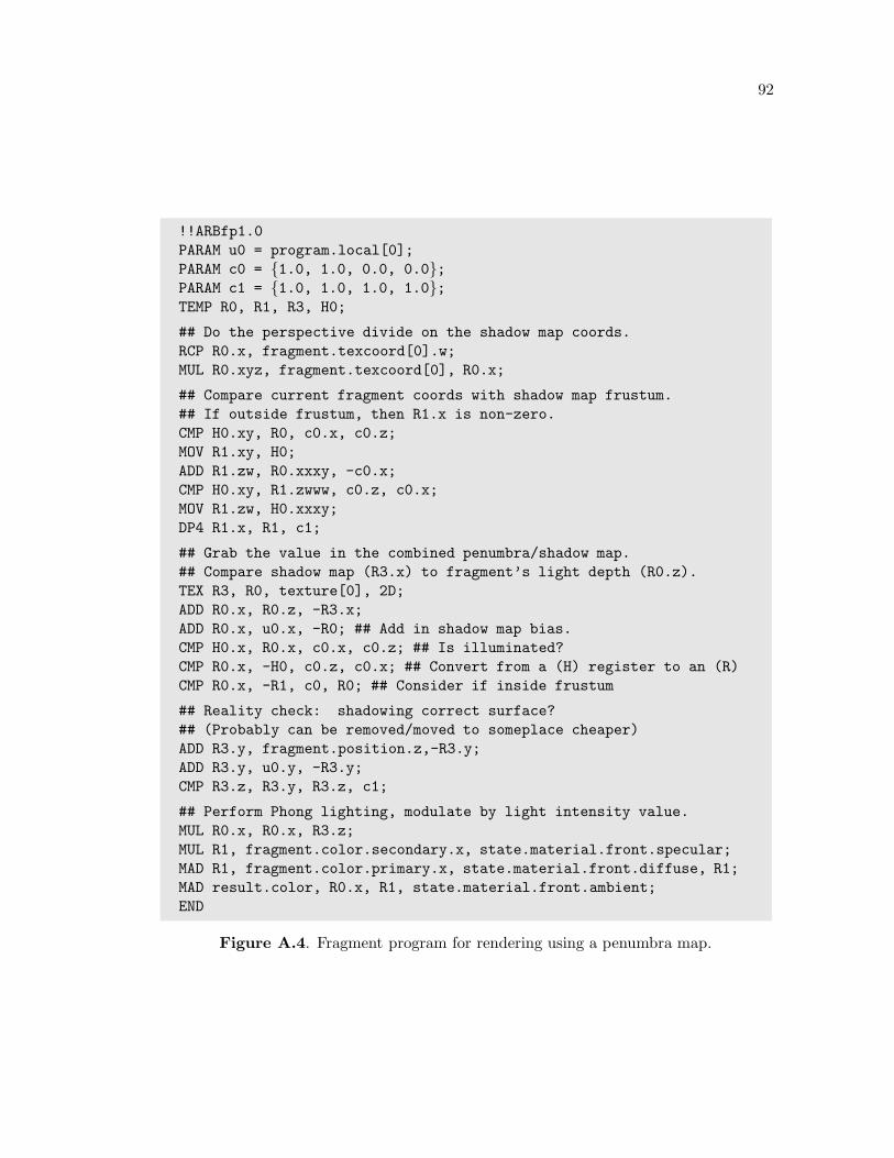
92
!!ARBfp1.0
PARAM u0 = program.local[0];
PARAM c0 = 1.0, 1.0, 0.0, 0.0;PARAM c1 = 1.0, 1.0, 1.0, 1.0;TEMP R0, R1, R3, H0;
## Do the perspective divide on the shadow map coords.
RCP R0.x, fragment.texcoord[0].w;
MUL R0.xyz, fragment.texcoord[0], R0.x;
## Compare current fragment coords with shadow map frustum.
## If outside frustum, then R1.x is non-zero.
CMP H0.xy, R0, c0.x, c0.z;
MOV R1.xy, H0;
ADD R1.zw, R0.xxxy, -c0.x;
CMP H0.xy, R1.zwww, c0.z, c0.x;
MOV R1.zw, H0.xxxy;
DP4 R1.x, R1, c1;
## Grab the value in the combined penumbra/shadow map.
## Compare shadow map (R3.x) to fragment’s light depth (R0.z).
TEX R3, R0, texture[0], 2D;
ADD R0.x, R0.z, -R3.x;
ADD R0.x, u0.x, -R0; ## Add in shadow map bias.
CMP H0.x, R0.x, c0.x, c0.z; ## Is illuminated?
CMP R0.x, -H0, c0.z, c0.x; ## Convert from a (H) register to an (R)
CMP R0.x, -R1, c0, R0; ## Consider if inside frustum
## Reality check: shadowing correct surface?
## (Probably can be removed/moved to someplace cheaper)
ADD R3.y, fragment.position.z,-R3.y;
ADD R3.y, u0.y, -R3.y;
CMP R3.z, R3.y, R3.z, c1;
## Perform Phong lighting, modulate by light intensity value.
MUL R0.x, R0.x, R3.z;
MUL R1, fragment.color.secondary.x, state.material.front.specular;
MAD R1, fragment.color.primary.x, state.material.front.diffuse, R1;
MAD result.color, R0.x, R1, state.material.front.ambient;
END
Figure A.4. Fragment program for rendering using a penumbra map.

APPENDIX B
SPHERICAL HARMONICS
Spherical harmonics provide an orthogonal basis for functions defined on a unit
sphere. As global illumination deals with incident and exitant energies over spheres and
hemispheres, spherical harmonics are a natural basis for representing these functions. A
number of researchers [14, 106, 107, 108, 117, 119, 120] have used spherical harmonic
coefficients to store illumination values, though few take time to clearly describe the
mathematics supporting the approach or describe implementational details. Hence, ac-
tually implementing their techniques requires significant background reading of cryptic
mathematics texts.
B.1 Laplace’s Equation in Spherical Coordinates
A harmonic is a function that satisfies Laplace’s equation:
∇2ϕ = 0. (B.1)
In spherical coordinates, Laplace’s equation becomes:[
1
r2
∂
∂r
(
r2 ∂
∂r
)
+1
r2 sin2 θ
∂2
∂φ2+
1
r2 sin θ
∂
∂θ
(
sin θ∂
∂θ
)]
ϕ = 0. (B.2)
By using separation of variables, where ϕ = R(r)Φ(φ)Θ(θ) and eliminating the 1r2 factor:
Θ(θ)Φ(φ)∂
∂r
(
r2 ∂R(r)
∂r
)
+Θ(θ)
sin2 θ
∂2Φ(φ)
∂φ2+
Φ(φ)
sin θ
∂
∂θ
(
sin θ∂Θ(θ)
∂θ
)
= 0. (B.3)
By dividing through by Φ(φ)Θ(θ), the r-dependence is reduced to a single term:
∂
∂r
(
r2 ∂R(r)
∂r
)
+1
Φ(φ) sin2 θ
∂2Φ(φ)
∂φ2+
1
Θ(θ) sin θ
∂
∂θ
(
sin θ∂Θ(θ)
∂θ
)
= 0. (B.4)
As the r-dependent terms and the r-independent terms are constant relative to each
other and sum to zero, equating the r-dependent term to a constant (of the form l(l + 1) [5])
gives:∂
∂r
(
r2 ∂R(r)
∂r
)
= l(l + 1). (B.5)

94
Substituting Equation B.5 back into Equation B.4 eliminates the dependency on r,
resulting in the spherical harmonic differential equation:
l(l + 1)Φ(φ)Θ(θ) +Θ(θ)
sin2 θ
∂2Φ(φ)
∂φ2+
Φ(φ)
sin θ
∂
∂θ
(
sin θ∂Θ(θ)
∂θ
)
= 0. (B.6)
The solutions to Equation B.6 are called spherical harmonics, and can be computed by
continuing the separation of variables. Multiplying by sin2 θΦ(φ)Θ(θ) reduces φ-dependency to
a single term, which again can be equated to a constant (typically called −m2):
1
Φ(φ)
∂2Φ(φ)
∂φ2= −m2, (B.7)
which has solutions:
Φ(φ) = Ae−imφ + Beimφ. (B.8)
Plugging Equation B.7 back into Equation B.6 gives an equation dependent on only θ:
l(l + 1) sin2 θ − m2 +sin θ
Θ(θ)
∂
∂θ
(
sin θ∂Θ(θ)
∂θ
)
= 0. (B.9)
And by replacing cos θ with x, and ∂θ with ∂x− sin θ , Equation B.9 becomes:
∂
∂x
[
(1 − x2)∂Θ
∂x
]
+
[
l(l + 1) − m2
1 − x2
]
Θ = 0. (B.10)
Equation B.10 is known as the associate Legendre differential equation, which has solu-
tions [5, 13]:
Θ(θ) = P ml (cos θ), −l ≤ m ≤ l for l,m ∈ Z. (B.11)
Here P ml (x) are the associated Legendre polynomials, discussed further in Section B.2.
Combining the solutions for Φ(φ) and Θ(θ) with a normalization factor gives a solution
for the angular portion of Laplace’s Equation in spherical coordinates. These are the
spherical harmonics Y ml (θ, φ), defined for θ ∈ [0, π] and φ ∈ [0, 2π) as:
Y ml (θ, φ) ≡
√
2l + 1
4π
(l − m)!
(l + m)!Pm
l (cos θ)eimφ, (B.12)
here the normalization constant√
2l+14π
(l−m)!(l+m)! is chosen such that
∫ 2π
0
∫ π
0Y m1
l1(θ, φ)Y m2
l2(θ, φ) sin θdθdφ = δm1 ,m2
δl1,l2 , (B.13)
with z defined as the complex conjugate of z.

95
B.2 Legendre Polynomials
Legendre polynomials are the solution to the Legendre differential equation, which is
a second-order ordinary differential equation of the form:
(1 − x2)∂2y
∂x2− 2x
∂y
∂x+ l(l + 1)y =
∂
∂x
[
(1 − x2)∂y
∂x
]
+ l(l + 1)y = 0, (B.14)
which is a special case of the associated Legendre differential equation given in Equa-
tion B.10, where m = 0. The solutions to Equations B.10 and B.14 are P ml (x) and Pl(x),
respectively the associated and unassociated Legendre functions. When l,m ∈ Z and
x ∈ R these functions become polynomial.
Interestingly, these functions have many representations, allowing for significant im-
plementational freedom to choose between speed and accuracy. Legendre polynomials are
special cases of hypergeometric functions pFq, such that:
Pl(x) = 2F1(−l, l + 1; 1;1
2(1 − x)) =
∞∑
n=0
(−l)n(l + 1)n
n!
(12 (1 − x))n
n!, (B.15)
where (a)b is the rising factorial defined as (a)b = a(a + 1) · · · (a + b − 1). Note that this
sum converges, as (−l)n spans zero for n > l. Alternately, the Rodrigues representation
yields a generating function for Pl(x) [148] which expands to:
Pl(x) =1
2l
bl/2c∑
k=0
(−1)k(2l − 2k)!
k!(l − k)!(l − 2k)!xl−2k =
1
2l
b1/2c∑
k=0
(−1)k
(
l
k
)(
2l − 2k
l
)
xl−2k. (B.16)
Finally, the Legendre polynomials satisfy the following recurrence relations, with
Equation B.18 providing more numerical stability for computational implementations [5]:
Pl+1(x) =(2l + 1)x
l + 1Pl(x) − l
l + 1Pl−1(x) (B.17)
= 2xPl(x) − Pl−1(x) − xPl(x) − Pl−1(x)
l − 1. (B.18)
The associated Legendre polynomials can be written in terms of the unassociated
polynomials. As long as l ≥ 0 and 0 ≤ m ≤ l:
Pml (x) = (−1)m(1 − x2)m/2 ∂m
∂xmPl(x). (B.19)
The polynomials with negative m values correspond to the polynomials with positive m
via the following identity:
P−ml (x) = (−1)m (l − m)!
(l + m)!Pm
l (x). (B.20)
Equations B.19 and B.20 provide a framework to compute the spherical harmonic basis
functions, but this approach is computationally infeasible due to the mth partial deriva-
tives used in Equation B.19. Luckily another representation exists for the associated

96
Legendre polynomials. Four relations allow easy computation of all associated Legendre
polynomials with m > 0:
Pml+1(x) =
x(2l + 1)
l − m + 1Pm
l (x) − l + m
l − m + 1Pm
l−1, (B.21)
Pm+1l (x) =
2mx√1 − x2
Pml (x) + [m(m − 1) − l(l + 1)] P m−1
l , (B.22)
P ll+1(x) = x(2l + 1)P l
l (x), (B.23)
P ll (x) = (−1)l(2l − 1)!!(1 − x2)
1
2 . (B.24)
Not all four relations are necessary to compute P ml for all m, l, but choosing relations for a
particular application can reduce discretization error. Only two equations are necessary to
compute all P ml , though Green [43] suggests combining Equations B.21, B.23, and B.24
to reduce errors for spherical harmonic based illumination. In Equation B.24, n!! is
the double factorial, defined for positive integers. For n odd, n!! = n · (n − 2) · · · 5 · 3 · 1,
and for n even, n!! = n · (n − 2) · · · 6 · 4 · 2. Two special cases are defined, which makes
computation of n!! easy, as −1!! ≡ 0!! ≡ 1.
To find the associated Legendre polynomials with negative m, use the relation:
P−ml (x) = (−1)m (l − m)!
(l + m)!Pm
l (x). (B.25)
Another useful identity, particularly when finding the spherical harmonic normaliza-
tion factor using Equation B.13, shows how to integrate the product of two associated
Legendre polynomials:∫ 1
−1Pm
l1 (x)P ml2 (x)dx =
2δl1,l2(l1 + m)!
(2l1 + 1)(l1 − m)!=
2δl1,l2(l2 + m)!
(2l2 + 1)(l2 − m)!. (B.26)
B.3 Spherical Harmonics
Spherical harmonics functions Y ml (θ, φ) are the angular portion of the solution to
Laplace’s equation in spherical coordinates (Equation B.2). They represent an infinite
set of orthogonal functions over the sphere. In fact, any function f(θ, φ) over the unit
sphere can be represented in terms of the complex spherical harmonic basis:
f(θ, φ) ≡∞
∑
l=0
l∑
m=−l
Aml Y m
l (θ, φ), (B.27)
where Aml are the spherical harmonic coefficients. The function f(θ, φ) can also be written
in terms of the real spherical harmonic basis functions:
f(θ, φ) ≡∞∑
l=0
l∑
m=0
[
Cml Y mc
l (θ, φ) + Sml Y ms
l (θ, φ)]
. (B.28)

97
The representation in Equation B.28 is a Laplace series, which is a generalized Fourier
series. In this sense, spherical harmonics are analogous to the Fourier basis in one
dimension. Here Y mc
l and Y ms
l are respectively the real and imaginary parts of Y ml :
Y mc
l ≡√
2l + 1
4π
(l − m)!
(l + m)!Pm
l (cos θ) cos(mφ), (B.29)
Y ms
l ≡√
2l + 1
4π
(l − m)!
(l + m)!Pm
l (cos θ) sin(mφ). (B.30)
Generally, the single symbol Y ml (x) is used in global illumination literature to repre-
sent the real spherical harmonic functions instead of a pair of symbols, such as Y mc
l (x)
and Y ms
l (x). To understand the illumination definition, realize that Equation B.28 could
easily be rewritten:
f(θ, φ) =
∞∑
l=0
[
l∑
m=0
Cml Y mc
l (θ, φ) +
0∑
m=−l
S|m|l Y
|m|sl (θ, φ)
]
. (B.31)
Thus, the real form of the spherical harmonics are typically written in cases, such that:
Y ml (θ, φ) =
√
2l + 1
2π
(l − m)!
(l + m)!Pm
l (cos θ) cos(mφ) if m > 0
√
2l + 1
4πP 0
l (cos θ) if m = 0√
2l + 1
2π
(l − |m|)!(l + |m|)!P
ml (cos θ) sin(|m|φ) if m < 0
. (B.32)
Notice the normalization factor has changed from the case of complex spherical harmonics.
Here the normalization factors have once again been chosen to satisfy Equation B.13. In
the rest of this chapter, Y ml refers to a real spherical harmonic basis function, as defined
in Equation B.32.
B.4 Using Spherical Harmonics Bases
By approximating a spherical function using a finite sum of the form:
f(θ, φ) =∞
∑
l=0
l∑
m=−l
Cml Y m
l (θ, φ) ≈n−1∑
l=0
l∑
m=−l
Cml Y m
l (θ, φ),
a low frequency function can easily be represented with a few Cml coefficients instead of a
more complex form, like an environment map. But the real advantage of using a spherical
harmonic basis, particularly for lighting computations, is the property that integration of

98
two functions simplifies to a dot product of their spherical harmonic coefficients C ml . In
other words, if f has spherical harmonic coefficients aml and g has coefficients bm
l then:
∫
θ,φf(θ, φ)g(θ, φ)dθdφ =
∞∑
l=0
l∑
m=−l
aml bm
l ≈n−1∑
l=0
l∑
m=−l
aml bm
l =
n2
∑
i=0
aibi. (B.33)
Often for ease of use, coefficients are represented with a single dimensional array ai instead
of a two-dimensional array aml . In this case, i = l(l+1)+m, and the sum above simplifies
to a summation over i. Typically, an nth order spherical harmonic representation is taken
to include the bands l = 0 . . . n − 1 and requires n2 coefficients. For clarity of notation
when using ai, Yi will be used for Y ml .
Finding the coefficients ai for function f is called projecting f into the spherical
harmonic basis. Projection is accomplished by integrating f over the sphere S with
respect to each basis function Yi:
ai =
∫
s∈S
f(s)Yi(s)ds. (B.34)
As f(θ, φ) often has no closed form solution or is defined on discrete samples (e.g., a
texture map), computing this integral numerically proves simpler in practice. Generally,
this is done using Monte Carlo integration [89]. By sampling randomly over the domain
of a function h, the Monte Carlo method approximates an integral by the sum:
∫
h(x)dx ≈ 1
N
N∑
i=1
h(xi)
p(xi), (B.35)
where N is the number of samples, and p(xi) is the probability density function of the
samples xi. Basically, this approach averages numerous samples over the domain of h to
approximate the integral. If nonuniform samples are used, or if the domain has non-unit
length, area, volume, etc., the probability density function accounts for the discrepancy.
For projecting a function f(θ, φ) into spherical harmonic coefficients, using a uniform
sampling over the sphere gives p(x) = 14π , as the surface area of a unit sphere is 4π.
Uniform samples over the surface of a sphere can be generated with two random variables
ξ1, ξ2 ∈ [0, 1] by [43]:
(θ, φ) =(
2 arccos(√
1 − ξ1), 2πξ2
)
(x, y, z) =(
2√
ξ1(1 − ξ1) cos(2πξ2), 2√
ξ1(1 − ξ1) sin(2πξ2), 1 − 2ξ1
)
.

99
For uniform samples over the hemisphere p(x) = 12π and the two random variables ξ1 and
ξ2 map to the hemisphere via [115]:
(θ, φ) =(
arccos(√
1 − ξ1), 2πξ2
)
(x, y, z) =(
√
ξ1 cos(2πξ2),√
ξ1 sin(2πξ2),√
1 − ξ1
)
. .
Consider the two spherical harmonic projected function f(s) and g(s) of order n,
where f has known coefficients ai and g has unknown coefficients bi. Should the need
arise to compute coefficients ci of the product h(s) = f(s)g(s), a transfer matrix F can
be derived such that:
ci =n2
∑
j=1
Fijbj . (B.36)
The elements of this matrix can be computed
Fij =
∫
s∈S
a(s)Yi(s)Yj(s)ds =n2
∑
k=0
ak
∫
s∈S
Yi(s)Yj(s)Yk(s)ds. (B.37)
These elements can be computed beforehand via numerical integration, or analytically:
∫ 2π
0
∫ π
0Y m1
l1(θ, φ)Y m2
l2(θ, φ)Y m3
l3(θ, φ) sin θdθdφ
=
√
(2l1 + 1)(2l2 + 1)(2l3 + 1)
4π
(
l1 l2 l30 0 0
)(
l1 l2 l3m1 m2 m3
)
,
where(
l1m1
l2m2
l3m3
)
is a Winger 3j-symbol [33, 148].
This property is commonly used for nondiffuse BRDFs, where three spherical harmonic
functions are used: one for the BRDF, one for the incident illumination, and one for the
transfer function describing self-shadowing and interreflections. In this case, changing
either the viewpoint or the illumination changes the rendered illumination, so two un-
knowns exist. For a single unknown, the dot product from Equation B.33 is sufficient,
but for two unknowns a transfer matrix is necessary.
Most importantly for interactive global illumination approaches, spherical harmonics
are rotationally invariant. This means a rotation before projection or an equivalent
rotation after projection give identical results. Since projection requires Monte Carlo
integration for most illumination functions, rotation of spherical harmonic coefficients
proves significantly faster. Unfortunately, rotation of coefficients is not as simple as
the 3 × 3 rotation matrix on the sphere. Rotation of nth order spherical harmonics

100
coefficients requires a n2 ×n2 rotation matrix, though the matrix is sparse as coefficients
from different bands do not interact. A spherical harmonic rotation matrix thus takes
the following form:
RSH =
1 0 0 0 0 0 0 0 0 · · ·0 0 0 0 0 0 · · ·0 R1
SH 0 0 0 0 0 · · ·0 0 0 0 0 0 · · ·0 0 0 0 · · ·0 0 0 0 · · ·0 0 0 0 R2
SH · · ·0 0 0 0 · · ·0 0 0 0 · · ·...
......
......
......
......
. . .
, (B.38)
where RiSH are (2i+1)× (2i+1) matrices which rotate the spherical harmonics of the ith
band. Using the rotation RS on the sphere, matrix elements can be computed as follows:
RSHij=
∫
s∈S
Yi(RS(s))Yj(s)ds. (B.39)
B.5 Computing Spherical HarmonicRotation Matrices
For rotations that are decomposed into ZY Z Euler angles, the matrix in Equa-
tion B.38 can be computed analytically as follows. If RS = RS(α,β,γ) = ZS(γ)YS(β)ZS(α)
can be decomposed into a rotation of α around the z-axis, a rotation of β around the
y-axis, and a rotation of γ around the z-axis, then RS(α,β,γ) can be rewritten:
RS(α,β,γ) = ZS(γ)XS(−π2)ZS(β)XS(+ π
2)ZS(α).
So it turns out only three matrices are necessary for an arbitrary rotation: one for a
general rotation about the z-axis and two constant matrices for rotation by ± π2 about
the x-axis. Fortunately, spherical harmonic rotation about the z-axis has a simple matrix:
ZSH(α) =
1 0 0 0 0 0 0 0 0 · · ·0 cos(α) 0 sin(α) 0 0 0 0 0 · · ·0 0 1 0 0 0 0 0 0 · · ·0 − sin(α) 0 cos(α) 0 0 0 0 0 · · ·0 0 0 0 cos(2α) 0 0 0 sin(2α) · · ·0 0 0 0 0 cos(α) 0 sin(α) 0 · · ·0 0 0 0 0 0 1 0 0 · · ·0 0 0 0 0 − sin(α) 0 cos(α) 0 · · ·0 0 0 0 − sin(2α) 0 0 0 cos(2α) · · ·...
......
......
......
......
. . .
.

101
As the number of bands increases, the nth order coefficient rotation matrix ZnSH(α) ex-
pands as expected, with terms of cos(α), cos(2α), . . . , cos(nα) and ± sin(α),± sin(2α), . . . ,
± sin(nα). The rotation around the x-axis by ± π2 can be described using the following
matrix:
XSH(±π2) =
1 0 0 0 0 0 0 0 0 · · ·0 0 ∓1 0 0 0 0 0 0 · · ·0 ±1 0 0 0 0 0 0 0 · · ·0 0 0 1 0 0 0 0 0 · · ·0 0 0 0 0 0 0 ∓1 0 · · ·0 0 0 0 0 −1 0 0 0 · · ·0 0 0 0 0 0 − 1
2 0 −√
32 · · ·
0 0 0 0 ±1 0 0 0 0 · · ·0 0 0 0 0 0 −
√3
2 0 12 · · ·
......
......
......
......
.... . .
.
These matrices give a straightforward method for arbitrarily rotating spherical har-
monic coefficients; however, ZY Z Euler angle decompositions may not fit well into all
applications. Additionally, performing five matrix multiply operations costs significantly
more than a single matrix multiplication, even with matrices as sparse as ZSH(α) and
XSH(±π2). These multiplications can be performed symbolically, but the resulting matrix
RSH(α,β,γ) contains some very complex trigonometric equations, which may prove more
difficult to store and evaluate than simply multiplying the five axis-aligned rotation
matrices.
However, recent research from the computational chemistry community [58, 59] has
led to the development of recurrence relations for building general rotation matrices,
without relying on Euler angle decompositions. Assuming an ordinary 3 × 3 rotation
matrix R defined as:
R =
Rxx Rxy Rxz
Ryx Ryy Ryz
Rzx Rzy Rzz
,
let[
Rs,t
]
be defined for −1 ≤ s, t ≤ 1 as:
[
Rs,t
]
=
Ryy Ryz Ryx
Rzy Rzz Rzx
Rxy Rxz Rxx
=
R−1,−1 R−1,0 R−1,1
R0,−1 R0,0 R0,1
R1,−1 R1,0 R1,1
. (B.40)
Let Mi ≡ RiSH (from Equation B.38) for notational clarity. Then for an nth order
spherical harmonic (i.e., 0 ≤ i < n and −i ≤ s, t ≤ i):
M is,t = ui
s,tUis,t + vi
s,tVis,t + wi
s,tWis,t. (B.41)

102
Here s and t are indices ranging over elements of the (2i+1) × (2i+1) rotation matrix
for the ith band of spherical harmonic coefficients. The coefficients u, v, w and functions
U, V,W,P appear in Tables B.1, B.2, and B.3 and define the recurrence relation. Note
these tables are from the original version of the Ivanic and Ruedenberg paper [58], which
contains erroneous equations but correct tables. The errata [59] fix the typos in the
relevant equations but introduce new ones into the table (for V is,t when s < 0). The table
in Green [43] contains a different typo for the same entry.
B.6 C++ Code to Compute the Rotation Matrix
This section contains a C++ class which computes the spherical harmonic rota-
tion matrix. The two functions visible to the rest of the program are the constructor
Table B.1. Definitions of numerical coefficients uis,t, vi
s,t, and wis,t.
Coefficient for |t| < i for |t| = i
uis,t:
√
(i+s)(i−s)(i+t)(i−t)
√
(i+s)(i−s)2i(2i−1)
vis,t:
12
√
(1+δs,0)(i+|s|−1)(i+|s|)(i+t)(i−t) (1 − 2δs,0)
12
√
(1+δs,0)(i+|s|−1)(i+|s|)2i(2i−1) (1 − 2δs,0)
wis,t: −1
2
√
(i−|s|−1)(i−|s|)(i+t)(i−t) (1 − δs,0) −1
2
√
(i−|s|−1)(i−|s|)2i(2i−1) (1 − δs,0)
Table B.2. Definitions of the functions U is,t, V i
s,t, and W is,t.
Function for s = 0 for s > 0 for s < 0
U is,t: 0P
i0,t 0P
is,t 0P
is,t
V is,t: 1P
i1,t + −1P
i−1,t 1P
is−1,t
√
1+δs,1 − 1Pis+1,t(1−δs,−1) +
−1Pi−s+1,t(1−δs,1) −1P
i−s+1,t
√
1+δs,−1
W is,t: (N/A, as wi
0,t = 0) 1Pis+1,t + −1P
i−s−1,t 1P
is−1,t + −1P
i−s+1,t
Table B.3. Definitions of the function rPis,t.
Function for |t| < i for t = i for t = −i
rPis,t: Rr,0M
i−1s,t Rr,1M
i−1s,i−1 − Rr,−1M
i−1s,−i+1 Rr,1M
i−1s,−i+1 + Rr,−1M
i−1s,i−1

103
SHRotationMatrix() and the function applyMatrix(), which applies the rotation matrix
to a vector of spherical harmonic coefficients.

104
// SHRotationMatrix Class Definition File
// --------------------------------------
// Takes a rotation matrix of the form:
// ( r[0], r[3], r[6] )
// ( r[1], r[4], r[7] ),
// ( r[2], r[5], r[8] )
// and an order. Computes an order2 ×order2 matrix.
class SHRotationMatrix private:
int order;
double inMatrix[9], *outMatrix;
// Computes the order2 ×order2 matrix
void computeMatrix( void );
// Compute an 1D index for (col,row) in the matrix
int matIndex( int col, int row );
// Computed as described in Table B.1.
double u i st ( int i, int s, int t );
double v i st ( int i, int s, int t );
double w i st ( int i, int s, int t );
// Computed as described in Table B.2.
double U i st ( int i, int s, int t );
double V i st ( int i, int s, int t );
double W i st ( int i, int s, int t );
// Computed as described in Table B.3.
double P r i st ( int r, int i, int s, int t );
// Index into the input matrix for −1 ≤ i, j ≤ 1, as per Eq. B.40
double R ( int i, int j );
// Index into band l, element (a,b) of the result (−l ≤ a, b ≤ l)double M( int l, int a, int b );
public:
// Constructor. Input: SH order & 3 × 3 transformation matrix
SHRotationMatrix( int order, double matrix[9] );
∼SHRotationMatrix();
// Applies the order2 ×order2 matrix to vector ’in’
void applyMatrix( double *in, double *out );
;
Figure B.1. Header file describing the SHRotationMatrix C++ class.

105
// Computes the uis,t coefficient, as per Table B.1
double SHRotationMatrix::u i st( int i, int s, int t )
return sqrt( (i+s)*(i-s) / ( abs(t)==i? 2*i*(2*i-1): (i+t)*(i-t) ) );
Figure B.2. Function definition for SHRotationMatrix::u i st().
// Computes the vis,t coefficient, as per Table B.1
double SHRotationMatrix::v i st( int i, int s, int t )
int delta = ( s==0 ? 1 : 0 );
double factor = 0.5 * (1 - 2*delta);
double numerator = (1+delta)*(i+abs(s)-1)*(i+abs(s));
double denominator = (abs(t)==i ? 2*i*(2*i-1) : (i+t)*(i-t));
return factor * sqrt( numerator / denominator );
Figure B.3. Function definition for SHRotationMatrix::v i st().
// Computes the wis,t coefficient, as per Table B.1
double SHRotationMatrix::w i st( int i, int s, int t )
int delta = ( s==0 ? 1 : 0 );
double factor = -0.5 * ( 1 - delta );
double numerator = (i-abs(s)-1)*(i-abs(s));
double denominator = (abs(t)==i ? 2*i*(2*i-1) : (i+t)*(i-t));
return factor * sqrt( numerator / denominator );
Figure B.4. Function definition for SHRotationMatrix::w i st().
// Computes the U is,t function, as per Table B.2
double SHRotationMatrix::U i st( int i, int s, int t )
return P r i st(0,i,s,t);
Figure B.5. Function definition for SHRotationMatrix::U i st().

106
// Computes the V is,t function, as per Table B.2
double SHRotationMatrix::V i st( int i, int s, int t )
int delta = ( abs(s)==1 ? 1 : 0 );
if ( s == 0 )
return P r i st(1,i,1,t) + P r i st(-1,i,-1,t);
if ( s > 0 )
return
sqrt(1+delta)*P r i st(1,i,s-1,t) - (1-delta)*P r i st(-1,i,-s+1,t);
return
(1-delta)*P r i st(1,i,s+1,t) + sqrt(1+delta)*P r i st(-1,i,-s-1,t);
Figure B.6. Function definition for SHRotationMatrix::V i st().
// Computes the W is,t function, as per Table B.2
double SHRotationMatrix::W i st( int i, int s, int t )
if ( s==0 ) return 0;
if ( s > 0 ) return P r i st(1,i,s+1,t) + P r i st(-1,i,-s-1,t);
return P r i st(1,i,s-1,t) - P r i st(-1,i,-s+1,t);
Figure B.7. Function definition for SHRotationMatrix::W i st().
// Computes the rPis,t function, as per Table B.3
double SHRotationMatrix::P r i st( int r, int i, int s, int t )
if (abs(t) < i) return R(r,0)*M(i-1,s,t);
if ( t == i ) return R(r,1)*M(i-1,s,i-1) - R(r,-1)*M(i-1,s,-i+1);
return R(r,1)*M(i-1,s,-i+1) + R(r,-1)*M(i-1,s,i-1);
Figure B.8. Function definition for SHRotationMatrix::P r i st().
// Ri,j indexes into the input matrix for −1 ≤ i, j ≤ 1// as per the definition of [Rs,t] (Eq. B.40)
double SHRotationMatrix::R( int i, int j )
int jp = ((j+2) % 3); // 0 ≤ jp < 3
int ip = ((i+2) % 3); // 0 ≤ ip < 3
return inMatrix[jp*3+ip]; // index into input matrix
Figure B.9. Function definition for SHRotationMatrix::R().

107
// Returns an element of the output matrix.
// l is the band of the matrix to reference 0 ≤ l < order// a and b are elements in the band, in the range [-l..l]
double SHRotationMatrix::M( int l, int a, int b )
if (l<=0) return outMatrix[0];
// Find the center of band l (outMatrix[ctr,ctr])
int ctr = l*(l+1);
return outMatrix[ matIndex( ctr + b, ctr + a ) ];
Figure B.10. Function definition for SHRotationMatrix::M().
// Find the index in the order2xorder2 output matrix
// for a given column and row
int SHRotationMatrix::matIndex( int col, int row )
return col*order*order+row;
Figure B.11. Function definition for SHRotationMatrix::matIndex().
// Setup the rotation matrix of a specified order given the equivalent
// 3 × 3 rotation transformation.
SHRotationMatrix::SHRotationMatrix( int order, double matrix[9] ):
order(order)
// Copy the input matrix into local storage.
for (int i=0;i<9;i++)
inMatrix[i] = matrix[i];
// allocate memory for SH rotation matrix.
outMatrix = new double[order*order*order*order];
// actually compute the matrix.
computeMatrix();
Figure B.12. Definition of constructor SHRotationMatrix::SHRotationMatrix().

108
// Assuming we know the input matrix, compute the SH rotation matrix
void SHRotationMatrix::computeMatrix( void )
// initialize the matrix to 0’s
for (int i=0;i<order*order;i++)
for (int j=0;j<order*order;j++)
outMatrix[matIndex(i,j)] = 0;
// 0th band (1× 1 matrix) is the identity
outMatrix[0] = 1;
if (order < 2) return;
// 1st band is a permutation of the 3D rotation matrix
for (int count=0, i=-1; i<=1; i++)
for (int j=-1; j<=1; j++)
outMatrix[ matIndex( (i+3)%3+1, (j+3)%3+1 ) ] = inMatrix[count++];
// 2nd+ bands use a recurrence relation.
for (int l=2;l<order;l++)
int ctr = l*(l+1);
for (int s=-l;s<=l;s++)
for (int t=-l;t<=l;t++)
outMatrix[ matIndex( ctr + t, ctr + s ) ] =
u i st( l, s, t ) * U i st( l, s, t ) +
v i st( l, s, t ) * V i st( l, s, t ) +
w i st( l, s, t ) * W i st( l, s, t );
Figure B.13. Function definition for SHRotationMatrix::computeMatrix().

109
// Applies the computed spherical harmonic rotation matrix
// in, out should contain order*order elements each.
// This does not do a full multiplication, rather only
// the (potentially) non-zero elements are multiplied.
void SHRotationMatrix::applyMatrix( double *in, double *out )
// first band (order 0) is a 1x1 identity rotation matrix
out[0] = in[0];
// set up data for multiplying 2nd band (order 1) coefs
int ord=1;
int minIdx=1;
int maxIdx=4;
// multiply the rest of the matrix
for (int idx=1; idx<order*order; idx++)
// multiply coefs from current band
out[idx]=0;
for (int j=minIdx;j<maxIdx;j++)
out[idx] += outMatrix[ matIndex( j, idx ) ] * in[j];
// increase the band, reset indices.
if (idx>=maxIdx-1)
ord++;
minIdx=maxIdx;
maxIdx+=2*ord+1;
Figure B.14. Function definition for SHRotationMatrix::applyMatrix().

REFERENCES
[1] Maneesh Agrawala, Ravi Ramamoorthi, Alan Heirich, and Laurent Moll. Efficientimage-based methods for rendering soft shadows. In Proceedings of SIGGRAPH,pages 375–384, 2000.
[2] Tomas Akenine-Moller and Ulf Assarsson. Approximate soft shadows on arbitrarysurfaces using penumbra wedges. In Proceedings of the Eurographics RenderingWorkshop, pages 309–318, 2002.
[3] Tomas Akenine-Moller and Eric Haines. Real-time Rendering. AK Peters, Mas-sachusetts, second edition, 2002.
[4] Arthur Appel. The notion of quantitative invisibility and machine rendering ofsolids. In Proceedings of the ACM National Conference, pages 387–393, 1967.
[5] George B. Arfken and Hans J. Weber. Mathematical Methods for Physicists.Academic Press, 4th edition edition, 1995.
[6] James Arvo. Backward ray tracing. Developments in Ray Tracing, pages 259–263,1986. ACM Siggraph ’86 Course Notes.
[7] James Arvo and David Kirk. Particle transport and image synthesis. In Proceedingsof SIGGRAPH, pages 63–66, 1990.
[8] Ian Ashdown. Radiosity: A Programmer’s Perspective. John Wiley & Sons, Inc.,1995.
[9] Ulf Assarsson and Tomas Akenine-Moller. A geometry-based soft shadow volumealgorithm using graphics hardware. ACM Transactions on Graphics, 22(3):511–520,July 2003.
[10] Kavita Bala, Julie Dorsey, and Seth Teller. Radiance interpolants for acceleratedbounded-error ray tracing. ACM Transactions on Graphics, 18(3):100–130, August1999.
[11] James F. Blinn. Models of light reflection for computer synthesized pictures. InProceedings of SIGGRAPH, pages 192–198, 1977.
[12] Stefan Brabec and Hans-Peter Seidel. Single sample soft shadows using depth maps.In Proceedings of Graphics Interface, pages 219–228, 2002.
[13] Willian E. Byerly. An Elementary Treatise on Fourier’s Series and Spherical, Cylin-drical, and Ellipsoidal Harmonics, with Applications to Problems in MathematicalPhysics. Ginn and Company, 1893.

111
[14] Brian Cabral, Nelson Max, and Rebecca Springmeyer. Bidirectional reflectionfunctions from surface bump maps. In Proceedings of SIGGRAPH, pages 273–281,1987.
[15] Brian Cabral, Marc Olano, and Philip Nemec. Reflection space image basedrendering. In Proceedings of SIGGRAPH, pages 165–170, 1999.
[16] Eric Chan and Fredo Durand. Rendering fake soft shadows with smoothies. InProceedings of the Eurographics Symposium on Rendering, pages 208–218, 2003.
[17] Subrahmanyan Chandrasekhar. Radiative Transfer. Oxford University Press, 1950.
[18] Min Chen and James Arvo. Theory and application of specular path perturbation.ACM Transactions on Graphics, 19(4):246–278, October 2000.
[19] Shenchang Eric Chen. Incremental radiosity: An extension of progressive radiosityto an interactive image synthesis system. In Proceedings of SIGGRAPH, pages135–144, 1990.
[20] Shenchang Eric Chen, Holly Rushmeier, Gavin Miller, and Douglass Turner. A pro-gressive multi-pass method for global illumination. In Proceedings of SIGGRAPH,pages 165–174, 1991.
[21] Michael Cohen, Shenchang Eric Chen, John Wallace, and Donald Greenburg. Aprogressive refinement approach to fast radiosity image generation. In Proceedingsof SIGGRAPH, pages 75–84, 1988.
[22] Michael Cohen and Donald Greenburg. The hemi-cube: A radiosity solution forcomplex environments. In Proceedings of SIGGRAPH, pages 31–40, 1985.
[23] Robert Cook, Thomas Porter, and Loren Carpenter. Distributed ray tracing. InProceedings of SIGGRAPH, pages 137–145, 1984.
[24] Robert L. Cook and Kenneth E. Torrance. A reflectance model for computergraphics. In Proceedings of SIGGRAPH, pages 307–316, 1981.
[25] Franklin Crow. Shadow algorithms for computer graphics. In Proceedings ofSIGGRAPH, pages 242–248, 1977.
[26] Paul E. Debevec and Jitendra Malik. Recovering high dynamic range radiancemaps from photographs. In Proceedings of SIGGRAPH, pages 369–378, 1997.
[27] David E Demarle, Steven Parker, Mark Hartner, Christiaan Gribble, and CharlesHansen. Distributed interactive ray tracing for large volume visualization. InProceedings of the IEEE Symposium on Parallel and Large-Data Visualization andGraphics, pages 87–94, 2003.
[28] Paul Diefenbach and Norman Badler. Multi-pass pipeline rendering: Realismfor dynamic environments. In Proceedings of the Symposium on Interactive 3DGraphics, pages 59–70, 1997.
[29] George Drettakis and Eugene Fiume. A fast shadow algorithm for area light sources

112
using backprojection. In Proceedings of SIGGRAPH, pages 223–230, 1994.
[30] George Drettakis and Francois X. Sillion. Interactive update of global illuminationusing a line-space hierarchy. In Proceedings of SIGGRAPH, pages 57–64, 1997.
[31] Philip Dutre and Yves Willems. Importance-driven monte carlo light tracing. InProceedings of the Eurographics Rendering Workshop, pages 188–197, 1994.
[32] Philip Dutre and Yves Willems. Potential-driven monte carlo particle tracing fordiffuse environments with adaptive probability functions. In Proceedings of theEurographics Rendering Workshop, pages 306–315, 1995.
[33] A. R. Edmonds. Angular Momentum in Quantum Mechanics. Princeton UniversityPress, 1957.
[34] Cass Everitt, Ashu Rege, and Cem Cabenoya. Hardware shadow mapping. Techni-cal report, nVidia, http://developer.nvidia.com/object/hwshadowmap paper.html,2001.
[35] Randima Fernando, Sebastian Fernandez, Kavita Bala, and Donald Greenberg.Adaptive shadow maps. In Proceedings of SIGGRAPH, pages 387–390, 2001.
[36] David Forsyth, Chien Yang, and Kim Teo. Efficient radiosity in dynamic environ-ments. In Proceedings of the Eurographics Rendering Workshop, pages 313–323,1994.
[37] David George, Francois Sillion, and Donald Greenberg. Radiosity redistributionfor dynamic environments. IEEE Computer Graphics & Applications, 10(4):26–34,July 1990.
[38] Cindy Goral, Kenneth Torrance, Donald Greenberg, and Bennett Battaile. Mod-elling the interaction of light between diffuse surfaces. In Proceedings of SIG-GRAPH, pages 213–222, 1984.
[39] Steven Gortler, Peter Schroder, Michael Cohen, and Pat Hanrahan. Waveletradiosity. In Proceedings of SIGGRAPH, pages 221–230, 1993.
[40] Henri Gouraud. Continuous shading of curved surfaces. IEEE Transactions onComputers, 20(6):623, June 1971.
[41] Xavier Granier and George Drettakis. Incremental updates for rapid glossy globalillumination. Computer Graphics Forum, 20(3):268–277, 2001.
[42] Xavier Granier, George Drettakis, and Bruce Walter. Fast global illuminationincluding specular effects. In Proceedings of the Eurographics Rendering Workshop,pages 47–59, 2000.
[43] Robin Green. Spherical harmonic lighting: The gritty details. In Archives of theGame Developers Conference, March 2003.
[44] Gene Greger, Peter Shirley, Philip Hubbard, and Donald Greenberg. The irradiancevolume. IEEE Computer Graphics & Applications, 18(2):32–43, March-April 1998.

113
[45] Eric Haines. Soft planar shadows using plateaus. Journal of Graphics Tools,6(1):19–27, 2001.
[46] Pat Hanrahan, David Salzman, and Larry Aupperle. A rapid hierarchical radiosityalgorithm. In Proceedings of SIGGRAPH, pages 197–206, 1991.
[47] David Hart, Philip Dutre, and Donald Greenberg. Direct illumination with lazyvisibility evaluation. In Proceedings of SIGGRAPH, pages 147–154, 1999.
[48] Paul Heckbert and Michael Herf. Simulating soft shadows with graphics hardware.Technical Report CMU-CS-97-104, Carnegie Mellon University, January 1997.
[49] Paul S. Heckbert. Adaptive radiosity textures for bidirectional ray tracing. InProceedings of SIGGRAPH, pages 145–154, 1990.
[50] Paul S. Heckbert. Discontinuity meshing for radiosity. In Proceedings of theEurographics Rendering Workshop, pages 203–216, 1992.
[51] Paul S. Heckbert. Simulating Global Illumination Using Adaptive Meshing. PhDthesis, UC Berkeley, California, June 1999.
[52] Paul S. Heckbert and Pat Hanrahan. Beam tracing polygonal objects. In Proceed-ings of SIGGRAPH, pages 119–127, 1984.
[53] Tim Heidmann. Real shadows, real time. Iris Universe, (18):23–31, November1991.
[54] Wolfgang Heidrich, Stefan Brabec, and Hans-Peter Seidel. Soft shadow maps forlinear lights. In Proceedings of the Eurographics Rendering Workshop, pages 269–280, 2000.
[55] Wolfgang Heidrich, Jan Kautz, Philipp Slusallek, and Hans-Peter Seidel. Cannedlightsources. In Proceedings of the Eurographics Rendering Workshop, pages 293–300, 1998.
[56] Helen Hu, Amy Gooch, William Thompson, Brian Smits, J. Rieser, and PeterShirley. Visual cues for imminent object contact in realistic virtual environments.In Proceedings of Visualization, pages 127–136, 2000.
[57] David Immel, Michael Cohen, and Donald Greenberg. A radiosity method fornon-diffuse environments. In Proceedings of SIGGRAPH, pages 133–142, 1986.
[58] Joseph Ivanic and Klaus Ruedenberg. Rotation matrices for real spherical har-monics, direct determination by recursion. Journal of Physical Chemistry A,100(15):6342–6347, 1996.
[59] Joseph Ivanic and Klaus Ruedenberg. Additions and corrections: Rotation matricesfor real spherical harmonics. Journal of Physical Chemistry A, 102(45):9099–9100,1998.
[60] Kei Iwasaki, Yoshinori Dobashi, and Tomoyuki Nishita. A fast rendering methodfor refractive and reflective caustics due to water surfaces. Computer Graphics

114
Forum, 22, 2003.
[61] Henrik Wann Jensen. Importance driven path tracing using the photon map. InProceedings of the Eurographics Rendering Workshop, pages 326–335, 1995.
[62] Henrik Wann Jensen. Rendering caustics on non-lambertian surfaces. In Proceed-ings of Graphics Interface, pages 116–121, 1996.
[63] Henrik Wann Jensen and Niels Jørgen Christensen. Efficiently rendering shadowsusing the photon map. In Proceedings of Compugraphics, December 1995.
[64] Henrik Wann Jensen and Niels Jørgen Christensen. Photon maps in bidirectionalmonte carlo ray tracing of complex objects. Computers & Graphics, 19(2):215–224,March 1995.
[65] Henrik Wann Jensen and Per H. Christensen. Efficient simulation of light trans-port in scenes with participating media using photon maps. In Proceedings ofSIGGRAPH, pages 311–320, 1998.
[66] Henrik Wann Jensen, Stephen R. Marschner, Marc Levoy, and Pat Hanrahan. Apractical model for subsurface light transport. In Proceedings of SIGGRAPH, pages511–518, 2001.
[67] James Kajiya. The rendering equation. In Proceedings of SIGGRAPH, pages 143–150, 1986.
[68] James Kajiya and Brian Von Herzen. Ray tracing volume densities. In Proceedingsof SIGGRAPH, pages 165–174, 1984.
[69] Arie E. Kaufman. Volume visualization in medicine. In Handbook of MedicalImaging, pages 713–730. Academic Press, 2000.
[70] Alexander Keller. Instant radiosity. In Proceedings of SIGGRAPH, pages 49–54,1997.
[71] Daniel Kersten, David C. Knill, Pascal Mamassian, and Isabelle Bulthoff. Illusorymotion from shadows. Nature, 279(6560):31, 1996.
[72] Daniel Kersten, Pascal Mamassian, and David C. Knill. Moving cast shadowsinduce apparent motion in depth. Perception, 26(2):171–192, 1997.
[73] Joe Kniss, Simon Premoze, Charles Hansen, Peter Shirley, and Allan McPherson.A model for volume lighting and modeling. IEEE Transactions on Visualizationand Computer Graphics, 9(2):150–162, April 2003.
[74] Eric Lafortune and Yves Willems. Bi-directional path tracing. In Proceedings ofCompugraphics, pages 145–153, 1993.
[75] Michael S. Langer and Heinrich H. Bulthoff. Depth discrimination from shadingunder diffuse lighting. Perception, 29:649–660, 2000.
[76] Barthold Lichtenbelt, Randy Crane, and Shaz Naqvi. Introduction to Volume

115
Rendering. Prentice Hall, 1st edition, 1998.
[77] Dani Lischinski, Filippo Tampieri, and Donald Greenberg. Discontinuity meshingfor accurate radiosity. IEEE Computer Graphics & Applications, 12(6):25–39,November 1992.
[78] Dani Lischinski, Filippo Tampieri, and Donald Greenberg. Combining hierarchicalradiosity and discontinuity meshing. In Proceedings of SIGGRAPH, pages 199–208,1993.
[79] William E. Lorensen and Harvey E. Cline. Marching cubes: A high resolution3d surface construction algorithm. In Proceedings of SIGGRAPH, pages 163–169,1987.
[80] Philippe Loutrel. A solution to the hidden-line problem for computer-drawnpolyhedra. IEEE Transactions on Computers, C-19(3):205–213, March 1970.
[81] Cindee Madison, Daniel Kersten, William Thompson, Peter Shirley, and BrianSmits. The use of subtle illumination cues for human judgement of spatial layout.Technical Report Technical Report UUCS-99-001, University of Utah, January1999.
[82] Thomas Malley. A shading method for computer generated images. Master’s thesis,Computer Science Department, University of Utah, June 1988.
[83] Stephen R. Marschner and Richard J. Lobb. An evaluation of reconstruction filterfor volume rendering. In Proceedings of Visualization, pages 100–107, October 1994.
[84] Nelson Max. Optical models for direct volume rendering. IEEE Transactions onVisualization and Computer Graphics, 1(2):99–108, 1995.
[85] Gregory M. Maxwell, Michael J. Bailey, and Victor W. Goldschmidt. Calculationsof the radiation configuration factor using ray casting. Computer-Aided Design,18(7):371–379, September 1986.
[86] Michael McCool. Shadow volume reconstruction from depth maps. ACM Transac-tions on Graphics, 19(1):1–26, January 2000.
[87] Gavin Miller. Efficient algorithms for local and global accessibility shading. InProceedings of SIGGRAPH, pages 319–326, 1994.
[88] Don Mitchell and Pat Hanrahan. Illumination from curved reflectors. In Proceed-ings of SIGGRAPH, pages 283–291, 1992.
[89] National Bureau of Standards. Monte carlo method. In A. S. Housholder, editor,Applied Mathematics Series 12, 1951.
[90] Ren Ng, Ravi Ramamoorthi, and Pat Hanrahan. All-frequency shadows using non-linear wavelet lighting approximation. ACM Transactions on Graphics, 22(3):376–381, 2003.
[91] Fred E. Nicodemus, Joseph C. Richmond, Jack J. Hsia, Irving W. Ginsberg, and

116
Thomas Limperis. Geometrical considerations and nomenclature for reflectance.Monograph 160. National Bureau of Standards, October 1977.
[92] Tomoyuki Nishita and Eihachiro Nakamae. Method of displaying optical effectswithin water using accumulation buffer. In Proceedings of SIGGRAPH, pages 373–381, 1994.
[93] J. F. Nye. Natural Focusing and Fine Structure of Light. Institute of PhysicsPublishing, Bristol, 1999.
[94] Eyal Ofek and Ari Rappoport. Interactive reflections on curved objects. InProceedings of SIGGRAPH, pages 333–342, 1999.
[95] Marc Ouellette and Eugene Fiume. Approximating the locaton of integranddiscontinuities for penumbral illumination with linear light sources. In Proceedingsof the Eurographics Rendering Workshop, pages 213–224, 1999.
[96] Steven Parker, William Martin, Peter-Pike Sloan, Peter Shirley, Brian Smits, andCharles Hansen. Interactive ray tracing. In Proceedings of the ACM Symposium onInteractive 3D Graphics, pages 119–126, 1999.
[97] Steven Parker, Michael Parker, Yarden Livnat, Peter-Pike Sloan, Charles Hansen,and Peter Shirley. Interactive ray tracing for volume visualization. IEEE Transac-tions on Visualization and Computer Graphics, 5(3):287–296, July 1999.
[98] Steven Parker, Peter Shirley, Yarden Livnat, Charles Hansen, and Peter-Pike Sloan.Interactive ray tracing for isosurface rendering. In Proceedings of Visualization,pages 233–238, October 1998.
[99] Steven Parker, Peter Shirley, and Brian Smits. Single sample soft shadows. Tech-nical Report Technical Report UUCS-98-019, University of Utah, October 1998.
[100] C. Alejandro Parraga, Tom Troscianko, and David J. Tolhurst. The human visualsystem is optimised for processing the spatial information in natural visual images.Current Biology, 10(1):35–38, January 2000.
[101] Sumanta Pattanaik and Sudhir Mudur. Adjoint equations and random walks forillumination computation. ACM Transactions on Graphics, 14(1):77–102, January1995.
[102] Bui-Thong Phong. Illumination for computer generated images. Communicationsof the ACM, 18:311–317, 1975.
[103] John F. Pile. Color in interior design. McGraw-Hill, New York, 1997.
[104] John F. Pile. Interior design. Harry N. Abrams, Inc., New York, 3rd. edition, 2003.
[105] Timothy Purcell, Craig Donner, Mike Cammarano, Henrik Wann Jensen, and PatHanrahan. Photon mapping on programmable graphics hardware. In Proceedingsof the SIGGRAPH/Eurographics Conference on Graphics Hardware, pages 41–50,2003.

117
[106] Ravi Ramamoorthi and Pat Hanrahan. An efficient representation for irradianceenvironment maps. In Proceedings of SIGGRAPH, pages 497–500, 2001.
[107] Ravi Ramamoorthi and Pat Hanrahan. A signal-processing framework for inverserendering. In Proceedings of SIGGRAPH, pages 117–128, 2001.
[108] Ravi Ramamoorthi and Pat Hanrahan. Frequency space environment map render-ing. In Proceedings of SIGGRAPH, pages 517–526, 2002.
[109] William Reeves, David Salesin, and Robert Cook. Rendering antialiased shadowswith depth maps. In Proceedings of SIGGRAPH, pages 283–291, 1987.
[110] Erik Reinhard, Peter Shirley, and Tom Troscianko. Natural image statistics forcomputer graphics. Technical Report UUCS-01-002, University of Utah, March2001.
[111] Holly Rushmeier, Charles Patterson, and Aravindan Veerasamy. Geometric simpli-fication for indirect illumination calculations. In Proceedings of Graphics Interface,pages 227–236, 1993.
[112] Will Schroeder, Ken Martin, and William Lorensen. The Visualization Toolkit: AnObject-Oriented Approach to 3D Graphics. Prentice Hall, 3rd edition, 2003.
[113] Mark Segal, Carl Korobkin, Rolf van Widenfelt, Jim Foran, and Paul Haeberli. Fastshadows and lighting effects using texture mapping. In Proceedings of SIGGRAPH,pages 249–252, 1992.
[114] Peter Shirley. A ray tracing method for illumination calculation in diffuse-specularscenes. In Proceedings of Graphics Interface, pages 205–212, 1990.
[115] Peter Shirley. Fundamentals of Computer Graphics. AK Peters, 2002.
[116] Silicon Graphics, Inc. OpenGL ARB Extension Registry. http://oss.sgi.com/projects/ogl-sample/registry/.
[117] Francois Sillion, James Arvo, Stephen Westin, and Donald Greenberg. A globalillumination solution for general reflectance distributions. In Proceedings of SIG-GRAPH, pages 187–196, 1991.
[118] Francois Sillion and Claude Puech. A general two-pass method integrating specularand diffuse reflection. In Proceedings of SIGGRAPH, pages 335–344, 1989.
[119] Peter-Pike Sloan, Jesse Hall, John Hart, and John Snyder. Clustered principalcomponents for precomputed radiance transfer. ACM Transactions on Graphics,22(3):382–391, 2003.
[120] Peter-Pike Sloan, Jan Kautz, and John Snyder. Precomputed radiance transferfor real-time rendering in dynamic, low-frequency lighting environments. ACMTransactions on Graphics, 21(3):527–536, 2002.
[121] Peter-Pike Sloan, Xingou Liu, Heung-Yeung Shum, and John Snyder. Bi-scaleradiance transfer. ACM Transactions on Graphics, 22(3):370–375, 2003.

118
[122] Brian Smits, James Arvo, and Donald Greenberg. A clustering algorithm forradiosity in complex environments. In Proceedings of SIGGRAPH, pages 435–442,1994.
[123] Brian Smits, James Arvo, and David Salesin. An importance-driven radiosityalgorithm. In Proceedings of SIGGRAPH, pages 273–282, 1992.
[124] Lisa M. Sobierajski and Arie E. Kaufman. Volumetric ray tracing. In Proceedingsof the Symposium on Volume Visualization, pages 11–18. ACM Press, 1994.
[125] Cyril Soler and Francois Sillion. Automatic calculation of soft shadow textures forfast, high quality radiosity. In Proceedings of the Eurographics Rendering Workshop,pages 199–210, 1998.
[126] Cyril Soler and Francois Sillion. Fast calculation of soft shadow texture usingconvolution. In Proceedings of SIGGRAPH, pages 321–332, 1998.
[127] Jos Stam. Random caustics: Natural textures and wave theory revisited. InSIGGRAPH Visual Proceedings, page 150. ACM Press, 1996.
[128] Jos Stam. Aperiodic texture mapping. Technical Report Research Report R046,ERCIM, January 1997.
[129] Marc Stamminger and George Drettakis. Perspective shadow maps. In Proceedingsof SIGGRAPH, pages 557–562, 2002.
[130] Michael Stark and Richard Riesenfeld. Exact illumination in polygonal envi-ronments using vertex tracing. In Proceedings of the Eurographics RenderingWorkshop, pages 149–160, 2000.
[131] A. James Stewart. Vicinity shading for enhanced perception of volumetric data. InProceedings of Visualization, pages 355–362, 2003.
[132] A. James Stewart and Sherif Ghali. Fast computation of shadow boundaries usingspatial coherence and backprojection. In Proceedings of SIGGRAPH, pages 231–238, 1994.
[133] Parag Tole, Fabio Pellacini, Bruce Walter, and Donald Greenberg. Interactiveglobal illumination in dynamic scenes. In Proceedings of SIGGRAPH, pages 537–546, 2002.
[134] Roy Troutman and Nelson L. Max. Radiosity algorithms using higher order finiteelement methods. In Proceedings of SIGGRAPH, pages 209–212, 1993.
[135] Tushar Udeshi and Charles Hansen. Towards interactive, photorealistic renderingof indoor scenes: A hybrid approach. In Proceedings of the Eurographics RenderingWorkshop, pages 63–76, 1999.
[136] Eric Veach and Leonidas J Guibas. Metropolis light transport. In Proceedings ofSIGGRAPH, pages 65–76, 1997.
[137] Ingo Wald, Carsten Benthin, and Philipp Slusallek. Interactive global illumination

119
in complex highly occluded environments. In Proceedings of the EurographicsSymposium on Rendering, pages 74–81, 2003.
[138] Ingo Wald, Thomas Kollig, Carsten Benthin, Alexander Keller, and PhilippSlusallek. Interactive global illumination using fast ray tracing. In Proceedingsof the Eurographics Rendering Workshop, pages 15–24, 2002.
[139] Ingo Wald, Philipp Slusallek, Carsten Benthin, and Markus Wagner. Interactiverendering with coherent ray tracing. Computer Graphics Forum, 20(3):153–164,2001.
[140] John Wallace, Michael Cohen, and Donald Greenberg. A two-pass solution tothe rendering equation: A synthesis of ray tracing and radiosity methods. InProceedings of SIGGRAPH, pages 311–320, 1987.
[141] John Wallace, Kells Elmquist, and Eric Haines. A ray tracing algorithm forprogressive radioisty. In Proceedings of SIGGRAPH, pages 335–344, 1989.
[142] Bruce Walter, George Drettakis, and Steven Parker. Interactive rendering usingthe render cache. In Proceedings of the Eurographics Rendering Workshop, pages19–30, June 1999.
[143] Michael Wand and Wolfgang Straßer. Real-time caustics. Computer GraphicsForum, 22(3):611–620, 2003.
[144] Leonard Wanger. The effect of shadow quality on the perception of spatialrelationships in computer generated imagery. In Proceedings of the Symposiumon Interactive 3D Graphics, pages 39–42, 1992.
[145] Leonard Wanger, James Ferwerda, and Donald Greenberg. Perceiving spatial rela-tionships in computer-generated images. IEEE Computer Graphics & Applications,12(3):44–58, May 1992.
[146] Gregory J. Ward, Francis M. Rubinstein, and Robert D. Clear. A ray tracingsolution for diffuse interreflection. In Proceedings of SIGGRAPH, pages 85–92,1988.
[147] Mark Watt. Light-water interaction using backward beam tracing. In Proceedingsof SIGGRAPH, pages 377–385, 1990.
[148] Eric W. Weisstein. CRC Concise Encyclopedia of Mathematics. CRC Press, 1999.
[149] Turner Whitted. An improved illumination model for shaded display. Communi-cations of the ACM, 23(6):343–349, June 1980.
[150] Lance Williams. Casting curved shadows on curved surfaces. In Proceedings ofSIGGRAPH, pages 270–274, 1978.
[151] Andrew Woo, Pierre Poulin, and Alain Fournier. A survey of shadow algorithms.IEEE Computer Graphics & Applications, 10(6):13–32, November 1990.
[152] Chris Wyman and Charles Hansen. Penumbra maps: Approximate soft shadows

120
in real-time. In Proceedings of the Eurographics Symposium on Rendering, pages202–207, 2003.
[153] Chris Wyman, Charles Hansen, and Peter Shirley. Interactive raytraced caustics.Technical Report Technical Report UUCS-03-009, University of Utah, April 2003.
[154] Harold R. Zatz. Galerkin radiosity: A higher order solution method for globalillumination. In Proceedings of SIGGRAPH, pages 213–220, August 1993.
[155] Sergej Zhukov, Andrej Iones, and Grigorij Kronin. An ambient light illuminationmodel. In Proceedings of the Eurographics Rendering Workshop, pages 45–56, 1998.