fast approximation of matrix coherence and …mmahoney/pubs/coherence...fast approximation of matrix...
TRANSCRIPT
Journal of Machine Learning Research 13 (2012) 3441-3472 Submitted 7/12; Published 12/12
Fast Approximation of Matrix Coherence and Statistical Leverage
Petros Drineas [email protected]
Malik Magdon-Ismail [email protected]
Department of Computer Science
Rensselaer Polytechnic Institute
Troy, NY 12180
Michael W. Mahoney [email protected]
Department of Mathematics
Stanford University
Stanford, CA 94305
David P. Woodruff [email protected]
IBM Almaden Research Center
650 Harry Road
San Jose, CA 95120
Editor: Mehryar Mohri
Abstract
The statistical leverage scores of a matrix A are the squared row-norms of the matrix containing
its (top) left singular vectors and the coherence is the largest leverage score. These quantities are
of interest in recently-popular problems such as matrix completion and Nystrom-based low-rank
matrix approximation as well as in large-scale statistical data analysis applications more gener-
ally; moreover, they are of interest since they define the key structural nonuniformity that must
be dealt with in developing fast randomized matrix algorithms. Our main result is a randomized
algorithm that takes as input an arbitrary n× d matrix A, with n≫ d, and that returns as output
relative-error approximations to all n of the statistical leverage scores. The proposed algorithm
runs (under assumptions on the precise values of n and d) in O(nd logn) time, as opposed to the
O(nd2) time required by the naıve algorithm that involves computing an orthogonal basis for the
range of A. Our analysis may be viewed in terms of computing a relative-error approximation to
an underconstrained least-squares approximation problem, or, relatedly, it may be viewed as an
application of Johnson-Lindenstrauss type ideas. Several practically-important extensions of our
basic result are also described, including the approximation of so-called cross-leverage scores, the
extension of these ideas to matrices with n≈ d, and the extension to streaming environments.
Keywords: matrix coherence, statistical leverage, randomized algorithm
1. Introduction
The concept of statistical leverage measures the extent to which the singular vectors of a matrix are
correlated with the standard basis and as such it has found usefulness recently in large-scale data
analysis and in the analysis of randomized matrix algorithms (Velleman and Welsch, 1981; Mahoney
and Drineas, 2009; Drineas et al., 2008). A related notion is that of matrix coherence, which has
been of interest in recently popular problems such as matrix completion and Nystrom-based low-
rank matrix approximation (Candes and Recht, 2008; Talwalkar and Rostamizadeh, 2010). Defined
c©2012 Petros Drineas, Malik Magdon-Ismail, Michael W. Mahoney and David P. Woodruff.
DRINEAS, MAGDON-ISMAIL, MAHONEY AND WOODRUFF
more precisely below, the statistical leverage scores may be computed as the squared Euclidean
norms of the rows of the matrix containing the top left singular vectors and the coherence of the
matrix is the largest statistical leverage score. Statistical leverage scores have a long history in
statistical data analysis, where they have been used for outlier detection in regression diagnostics
(Hoaglin and Welsch, 1978; Chatterjee and Hadi, 1986). Statistical leverage scores have also proved
crucial recently in the development of improved worst-case randomized matrix algorithms that are
also amenable to high-quality numerical implementation and that are useful to domain scientists
(Drineas et al., 2008; Mahoney and Drineas, 2009; Boutsidis et al., 2009; Drineas et al., 2006b;
Sarlos, 2006; Drineas et al., 2010b); see Mahoney (2011) for a detailed discussion. The naıve and
best previously existing algorithm to compute these scores would compute an orthogonal basis for
the dominant part of the spectrum of A, for example, the basis provided by the Singular Value
Decomposition (SVD) or a basis provided by a QR decomposition (Golub and Loan, 1996), and
then use that basis to compute diagonal elements of the projection matrix onto the span of that
basis.
We present a randomized algorithm to compute relative-error approximations to every statistical
leverage score in time qualitatively faster than the time required to compute an orthogonal basis. For
the case of an arbitrary n× d matrix A, with n≫ d, our main algorithm runs (under assumptions
on the precise values of n and d, see Theorem 2 for an exact statement) in O(nd logn/ε2) time, as
opposed to the Θ(nd2) time required by the naıve algorithm. As a corollary, our algorithm provides
a relative-error approximation to the coherence of an arbitrary matrix in the same time. In addition,
several practically-important extensions of the basic idea underlying our main algorithm are also
described in this paper.
1.1 Overview and Definitions
We start with the following definition of the statistical leverage scores of a matrix.
Definition 1 Given an arbitrary n×d matrix A, with n > d, let U denote the n×d matrix consisting
of the d left singular vectors of A, and let U(i) denote the i-th row of the matrix U as a row vector.
Then, the statistical leverage scores of the rows of A are given by
ℓi =∥
∥U(i)
∥
∥
2
2,
for i ∈ 1, . . . ,n; the coherence γ of the rows of A is
γ = maxi∈1,...,n
ℓi,
that is, it is the largest statistical leverage score of A; and the (i, j)-cross-leverage scores ci j are
ci j =⟨
U(i),U( j)
⟩
,
that is, they are the dot products between the ith row and the jth row of U.
Although we have defined these quantities in terms of a particular basis, they clearly do not depend
on that particular basis, but only on the space spanned by that basis. To see this, let PA denote the
projection matrix onto the span of the columns of A. Then,
ℓi =∥
∥U(i)
∥
∥
2
2=(
UUT)
ii= (PA)ii . (1)
3442
FAST APPROXIMATION OF MATRIX COHERENCE AND STATISTICAL LEVERAGE
That is, the statistical leverage scores of a matrix A are equal to the diagonal elements of the projec-
tion matrix onto the span of its columns.1 Similarly, the (i, j)-cross-leverage scores are equal to the
off-diagonal elements of this projection matrix, that is,
ci j = (PA)i j =⟨
U(i),U( j)
⟩
. (2)
Clearly, O(nd2) time suffices to compute all the statistical leverage scores exactly: simply perform
the SVD or compute a QR decomposition of A in order to obtain any orthogonal basis for the range
of A and then compute the Euclidean norm of the rows of the resulting matrix. Thus, in this paper,
we are interested in algorithms that run in o(nd2) time.
Several additional comments are worth making regarding this definition. First, since ∑ni=1 ℓi =
‖U‖2F = d, we can define a probability distribution over the rows of A as pi = ℓi/d. As discussed
below, these probabilities have played an important role in recent work on randomized matrix al-
gorithms and an important algorithmic question is the degree to which they are uniform or nonuni-
form.2 Second, one could also define leverage scores for the columns of a “tall” matrix A, but
clearly those are all equal to one unless n < d or A is rank-deficient. Third, and more generally,
given a rank parameter k, one can define the statistical leverage scores relative to the best rank-k
approximation to A to be the n diagonal elements of the projection matrix onto the span of Ak, the
best rank-k approximation to A.
1.2 Our Main Result
Our main result is a randomized algorithm for computing relative-error approximations to every
statistical leverage score, as well as an additive-error approximation to all of the large cross-leverage
scores, of an arbitrary n× d matrix, with n≫ d, in time qualitatively faster than the time required
to compute an orthogonal basis for the range of that matrix. Our main algorithm for computing
approximations to the statistical leverage scores (see Algorithm 1 in Section 3) will amount to
constructing a “randomized sketch” of the input matrix and then computing the Euclidean norms
of the rows of that sketch. This sketch can also be used to compute approximations to the large
cross-leverage scores (see Algorithm 2 of Section 3).
The following theorem provides our main quality-of-approximation and running time result for
Algorithm 1.
Theorem 2 Let A be a full-rank n× d matrix, with n≫ d; let ε ∈ (0,1/2] be an error parameter;
and recall the definition of the statistical leverage scores ℓi from Definition 1. Then, there exists a
randomized algorithm (Algorithm 1 of Section 3 below) that returns values ℓi, for all i ∈ 1, . . . ,n,such that with probability at least 0.8,
∣
∣ℓi− ℓi
∣
∣≤ εℓi
1. In this paper, for simplicity of exposition, we consider the case that the matrix A has rank equal to d, that is, has full
column rank. Theoretically, the extension to rank-deficient matrices A is straightforward—simply modify Definition 1
and thus Equations (1) and (2) to let U be any orthogonal matrix (clearly, with fewer than d columns) spanning the
column space of A. From a numerical perspective, things are substantially more subtle, and we leave this for future
work that considers numerical implementations of our algorithms.
2. Observe that if U consists of d columns from the identity, then the leverage scores are extremely nonuniform: d of
them are equal to one and the remainder are equal to zero. On the other hand, if U consists of d columns from a
normalized Hadamard transform (see Section 2.3 for a definition), then the leverage scores are very uniform: all n of
them are equal to d/n.
3443

DRINEAS, MAGDON-ISMAIL, MAHONEY AND WOODRUFF
holds for all i ∈ 1, . . . ,n. Assuming d ≤ n≤ ed , the running time of the algorithm is
O(
nd ln(
dε−1)
+ndε−2 lnn+d3ε−2 (lnn)(
ln(
dε−1)))
.
Algorithm 1 provides a relative-error approximation to all of the statistical leverage scores ℓi of A
and, assuming d lnd = o(
nlnn
)
, lnn = o(d), and treating ε as a constant, its running time is o(nd2),as desired. As a corollary, the largest leverage score (and thus the coherence) is approximated to
relative-error in o(nd2) time.
The following theorem provides our main quality-of-approximation and running time result for
Algorithm 2.
Theorem 3 Let A be a full-rank n× d matrix, with n≫ d; let ε ∈ (0,1/2] be an error parameter;
let κ be a parameter; and recall the definition of the cross-leverage scores ci j from Definition 1.
Then, there exists a randomized algorithm (Algorithm 2 of Section 3 below) that returns the pairs
(i, j) together with estimates ci j such that, with probability at least 0.8,
i. If c2i j ≥
d
κ+12εℓiℓ j, then (i, j) is returned; if (i, j) is returned, then c2
i j ≥d
κ−30εℓiℓ j.
ii. For all pairs (i, j) that are returned, c2i j−30εℓiℓ j ≤ c2
i j ≤ c2i j +12εℓiℓ j.
This algorithm runs in O(ε−2n lnn+ ε−3κd ln2 n) time.
Note that by setting κ = n lnn, we can compute all the “large” cross-leverage scores, that is, those
satisfying c2i j ≥ d
n lnn, to within additive-error in O
(
nd ln3 n)
time (treating ε as a constant). If ln3 n =
o(d) the overall running time is o(nd2), as desired.
1.3 Significance and Related Work
Our results are important for their applications to fast randomized matrix algorithms, as well as their
applications in numerical linear algebra and large-scale data analysis more generally.
Significance in theoretical computer science. The statistical leverage scores define the key struc-
tural nonuniformity that must be dealt with (i.e., either rapidly approximated or rapidly uniformized
at the preprocessing step) in developing fast randomized algorithms for matrix problems such as
least-squares regression (Sarlos, 2006; Drineas et al., 2010b) and low-rank matrix approximation
(Papadimitriou et al., 2000; Sarlos, 2006; Drineas et al., 2008; Mahoney and Drineas, 2009; Bout-
sidis et al., 2009). Roughly, the best random sampling algorithms use these scores (or the gener-
alized leverage scores relative to the best rank-k approximation to A) as an importance sampling
distribution to sample with respect to. On the other hand, the best random projection algorithms
rotate to a basis where these scores are approximately uniform and thus in which uniform sampling
is appropriate. See Mahoney (2011) for a detailed discussion.
As an example, the CUR decomposition of Drineas et al. (2008) and Mahoney and Drineas
(2009) essentially computes pi = ℓi/k, for all i ∈ 1, . . . ,n and for a rank parameter k, and it
uses these as an importance sampling distribution. The computational bottleneck for these and
related random sampling algorithms is the computation of the importance sampling probabilities.
On the other hand, the computational bottleneck for random projection algorithms is the application
of the random projection, which is sped up by using variants of the Fast Johnson-Lindenstrauss
Transform (Ailon and Chazelle, 2006, 2009). By our main result, the leverage scores (and thus
3444
FAST APPROXIMATION OF MATRIX COHERENCE AND STATISTICAL LEVERAGE
these probabilities) can be approximated in time that depends on an application of a Fast Johnson-
Lindenstrauss Transform. In particular, the random sampling algorithms of Drineas et al. (2006b),
Drineas et al. (2008) and Mahoney and Drineas (2009) for least-squares approximation and low-
rank matrix approximation now run in time that is essentially the same as the best corresponding
random projection algorithm for those problems (Sarlos, 2006).
Applications to numerical linear algebra. Recently, high-quality numerical implementations of
variants of the basic randomized matrix algorithms have proven superior to traditional determinis-
tic algorithms (Rokhlin and Tygert, 2008; Rokhlin et al., 2009; Avron et al., 2010). An important
question raised by our main results is how these will compare with an implementation of our main
algorithm. More generally, density functional theory (Bekas et al., 2007) and uncertainty quantifica-
tion (Bekas et al., 2009) are two scientific computing areas where computing the diagonal elements
of functions (such as a projection or inverse) of very large input matrices is common. For example,
in the former case, “heuristic” methods based on using Chebychev polynomials have been used in
numerical linear algebra to compute the diagonal elements of the projector (Bekas et al., 2007). Our
main algorithm should have implications in both of these areas.
Applications in large-scale data analysis. The statistical leverage scores and the scores rela-
tive to the best rank-k approximation to A are equal to the diagonal elements of the so-called “hat
matrix” (Hoaglin and Welsch, 1978; Chatterjee and Hadi, 1988). As such, they have a natural statis-
tical interpretation in terms of the “leverage” or “influence” associated with each of the data points
(Hoaglin and Welsch, 1978; Chatterjee and Hadi, 1986, 1988). In the context of regression prob-
lems, the ith leverage score quantifies the leverage or influence of the ith constraint/row of A on the
solution of the overconstrained least squares optimization problem minx ‖Ax−b‖2 and the (i, j)-thcross leverage score quantifies how much influence or leverage the ith data point has on the jth least-
squares fit (see Hoaglin and Welsch, 1978; Chatterjee and Hadi, 1986, 1988, for details). When
applied to low-rank matrix approximation problems, the leverage score ℓ j quantifies the amount of
leverage or influence exerted by the jth column of A on its optimal low-rank approximation. His-
torically, these quantities have been widely-used for outlier identification in diagnostic regression
analysis (Velleman and Welsch, 1981; Chatterjee et al., 2000).
More recently, these scores (usually the largest scores) often have an interpretation in terms of
the data and processes generating the data that can be exploited. For example, depending on the
setting, they can have an interpretation in terms of high-degree nodes in data graphs, very small
clusters in noisy data, coherence of information, articulation points between clusters, the value of
a customer in a network, space localization in sensor networks, etc. (Bonacich, 1987; Richardson
and Domingos, 2002; Newman, 2005; Jonckheere et al., 2007; Mahoney, 2011). In genetics, dense
matrices of size thousands by hundreds of thousands (a size scale at which even traditional deter-
ministic QR algorithms fail to run) constructed from DNA Single Nucleotide Polymorphisms (SNP)
data are increasingly common, and the statistical leverage scores can correlate strongly with other
metrics of genetic interest (Paschou et al., 2007; Mahoney and Drineas, 2009; Drineas et al., 2010a;
Paschou et al., 2010). Our main result will permit the computation of these scores and related quan-
tities for significantly larger SNP data sets than has been possible previously (Paschou et al., 2007;
Drineas et al., 2010a; Paschou et al., 2010; Georgiev and Mukherjee, 2011).
Remark. Lest there be any confusion, we should emphasize our main contributions. First,
note that statistical leverage and matrix coherence are important concepts in statistics and machine
learning. Second, recall that several random sampling algorithms for ubiquitous matrix problems
such as least-squares approximation and low-rank matrix approximation use leverage scores in a
3445

DRINEAS, MAGDON-ISMAIL, MAHONEY AND WOODRUFF
crucial manner; but until now these algorithms were Ω(TSV D), where TSV D is the time required to
compute a QR decomposition or a partial SVD of the input matrix. Third, note that, in some cases,
o(TSV D) algorithms exist for these problems based on fast random projections. But recall that the
existence of those projection algorithms in no way implies that it is easy or obvious how to compute
the statistical leverage scores efficiently. Fourth, one implication of our main result is that those
random sampling algorithms can now be performed just as efficiently as those random projection
algorithms; thus, the solution for those matrix problems can now be obtained while preserving the
identity of the rows. That is, these problems can now be solved just as efficiently by using actual
rows, rather than the arbitrary linear combinations of rows that are returned by random projections.
Fifth, we provide a generalization to “fat” matrices and to obtaining the cross-leverage scores. Sixth,
we develop algorithms that can compute leverage scores and related statistics even in streaming
environments.
1.4 Empirical Discussion of Our Algorithms
Although the main contribution of our paper is to provide a rigorous theoretical understanding of
fast leverage score approximation, our paper does analyze the theoretical performance of what is
meant to be a practical algorithm. Thus, one might wonder about the empirical performance of
our algorithms—for example, whether hidden constants render the algorithms useless for data of
realistic size. Not surprisingly, this depends heavily on the quality of the numerical implementation,
whether one is interested in “tall” or more general matrices, etc. We will consider empirical and
numerical aspects of these algorithms in forthcoming papers, for example, Gittens and Mahoney
(2012). We will, however, provide here a brief summary of several numerical issues for the reader
interested in these issues.
Empirically, the running time bottleneck for our main algorithm (Algorithm 1 of Section 3)
applied to “tall” matrices is the application of the random projection Π1. Thus, empirically the
running time is similar to the running time of random projection based methods for computing
approximations to the least-squares problem, which is also dominated by the application of the
random projection. The state of the art here is the Blendenpik algorithm of Avron et al. (2010)
and the LSRN algorithm of Meng et al. (2011). In their Blendenpik paper, Avron, Maymounkov,
and Toledo showed that their high-quality numerical implementation of a Hadamard-based random
projection (and associated least-squares computation) “beats LAPACK’s3 direct dense least-squares
solver by a large margin on essentially any dense tall matrix,” and they concluded that their empir-
ical results “suggest that random projection algorithms should be incorporated into future versions
of LAPACK” (Avron et al., 2010). The LSRN algorithm of Meng, Saunders, and Mahoney im-
proves Blendenpik in several respects, for example, providing better handling of sparsity and rank
deficiency, but most notably the random projection underlying LSRN is particularly appropriate for
solving large problems on clusters with high communication cost, for example, it has been shown
to scale well on Amazon Elastic Cloud Compute clusters. Thus, our main algorithm should extend
easily to these environments with the use of the random projection underlying LSRN. Moreover, for
both Blendenpik and LSRN (when implemented with a Hadamard-based random projection), the
hidden constants in the Hadamard-based random projection are so small that the random projection
algorithm (and thus the empirical running time of our main algorithm for approximating leverage
3. LAPACK (short for Linear Algebra PACKage) is a high-quality and widely-used software library of numerical routines
for solving a wide range of numerical linear algebra problems.
3446
FAST APPROXIMATION OF MATRIX COHERENCE AND STATISTICAL LEVERAGE
scores) beats the traditional O(nd2) time algorithm for dense matrices as small as thousands of rows
by hundreds of columns.
1.5 Outline
In Section 2, we will provide a brief review of relevant notation and concepts from linear algebra.
Then, in Sections 3 and 4, we will present our main results: Section 3 will contain our main al-
gorithm and Section 4 will contain the proof of our main theorem. Section 5 will then describe
extensions of our main result to general “fat” matrices, that is, those with n ≈ d. Section 6 will
conclude by describing the relationship of our main result with another related estimator for the sta-
tistical leverage scores, an application of our main algorithm to the under-constrained least-squares
approximation problem, and extensions of our main algorithm to streaming environments.
2. Preliminaries on Linear Algebra and Fast Random Projections
We will start with a review of basic linear algebra and notation, and then we will describe the Fast
Johnson-Lindenstrauss Transform and the related Subsampled Randomized Hadamard Transform.
2.1 Basic Linear Algebra and Notation
Let [n] denote the set of integers 1,2, . . . ,n. For any matrix A ∈ Rn×d , let A(i), i ∈ [n], denote
the i-th row of A as a row vector, and let A( j), j ∈ [d] denote the j-th column of A as a column
vector. Let ‖A‖2F = ∑n
i=1 ∑dj=1 A2
i j denote the square of the Frobenius norm of A, and let ‖A‖2 =sup ‖x‖2=1 ‖Ax‖2 denote the spectral norm of A. Relatedly, for any vector x∈Rn, its Euclidean norm
(or ℓ2-norm) is the square root of the sum of the squares of its elements. The dot product between
two vectors x,y∈Rn will be denoted 〈x,y〉, or alternatively as xT y. Finally, let ei ∈Rn, for all i∈ [n],denote the standard basis vectors for Rn and let In denote the n×n identity matrix.
Let the rank of A be ρ≤minn,d, in which case the “compact” or “thin” SVD of A is denoted
by A = UΣV T , where U ∈ Rn×ρ, Σ ∈ R
ρ×ρ, and V ∈ Rd×ρ. (For a general matrix X , we will
write X = UX ΣXV TX .) Let σi(A), i ∈ [ρ] denote the i-th singular value of A, and let σmax(A) and
σmin(A) denote the maximum and minimum singular values of A, respectively. The Moore-Penrose
pseudoinverse of A is the d× n matrix defined by A† = V Σ−1UT (Nashed, 1976). Finally, for any
orthogonal matrix U ∈Rn×ℓ, let U⊥ ∈R
n×(n−ℓ) denote an orthogonal matrix whose columns are an
orthonormal basis spanning the subspace of Rn that is orthogonal to the subspace spanned by the
columns of U (i.e., the range of U). It is always possible to extend an orthogonal matrix U to a full
orthonormal basis of Rn as [U U⊥].
The SVD is important for a number of reasons (Golub and Loan, 1996). For example, the
projection of the columns of A onto the k left singular vectors associated with the top k singular
values gives the best rank-k approximation to A in the spectral and Frobenius norms. Relatedly,
the solution to the least-squares (LS) approximation problem is provided by the SVD: given an
n× d matrix A and an n-vector b, the LS problem is to compute the minimum ℓ2-norm vector x
such that ‖Ax−b‖2 is minimized over all vectors x ∈ Rd . This optimal vector is given by xopt =
A†b. We call a LS problem overconstrained (or overdetermined) if n > d and underconstrained (or
underdetermined) if n < d.
3447

DRINEAS, MAGDON-ISMAIL, MAHONEY AND WOODRUFF
2.2 The Fast Johnson-Lindenstrauss Transform (FJLT)
Given ε> 0 and a set of points x1, . . . ,xn with xi ∈Rd , a ε-Johnson-Lindenstrauss Transform (ε-JLT),
denoted Π ∈ Rr×d , is a projection of the points into R
r such that
(1− ε)‖xi‖22 ≤ ‖Πxi‖2
2 ≤ (1+ ε)‖xi‖22.
To construct an ε-JLT with high probability, simply choose every entry of Π independently, equal
to ±√
3/r with probability 1/6 each and zero otherwise (with probability 2/3) (Achlioptas, 2003).
Let ΠJLT be a matrix drawn from such a distribution over r× d matrices.4 Then, the following
lemma holds.
Lemma 4 (Theorem 1.1 of Achlioptas (2003)) Let x1, . . . ,xn be an arbitrary (but fixed) set of points,
where xi ∈ Rd and let 0 < ε≤ 1/2 be an accuracy parameter. If
r ≥ 1
ε2
(
12lnn+6ln1
δ
)
then, with probability at least 1−δ, ΠJLT ∈ Rr×d is an ε-JLT .
For our main results, we will also need a stronger requirement than the simple ε-JLT and so we will
use a version of the Fast Johnson-Lindenstrauss Transform (FJLT), which was originally introduced
in Ailon and Chazelle (2006) and Ailon and Chazelle (2009). Consider an orthogonal matrix U ∈R
n×d , viewed as d vectors in Rn. A FJLT projects the vectors from R
n to Rr, while preserving the
orthogonality of U ; moreover, it does so very quickly. Specifically, given ε > 0, Π ∈ Rr×n is an
ε-FJLT for U if
•∥
∥Id−UT ΠT ΠU∥
∥
2≤ ε, and
• given any X ∈ Rn×d , the matrix product ΠX can be computed in O(nd lnr) time.
The next lemma follows from the definition of an ε-FJLT, and its proof can be found in Drineas
et al. (2006b) and Drineas et al. (2010b).
Lemma 5 Let A be any matrix in Rn×d with n≫ d and rank(A) = d. Let the SVD of A be A =
UΣV T , let Π be an ε-FJLT for U (with 0 < ε ≤ 1/2) and let Ψ = ΠU = UΨΣΨV TΨ . Then, all the
following hold:
rank(ΠA) = rank(ΠU) = rank(U) = rank(A) = d,∥
∥I−Σ−2Ψ
∥
∥
2≤ ε/(1− ε), and (3)
(ΠA)† = V Σ−1(ΠU)†. (4)
4. When no confusion can arise, we will use ΠJLT to refer to this distribution over matrices as well as to a specific
matrix drawn from this distribution.
3448

FAST APPROXIMATION OF MATRIX COHERENCE AND STATISTICAL LEVERAGE
2.3 The Subsampled Randomized Hadamard Transform (SRHT)
One can use a Randomized Hadamard Transform (RHT) to construct, with high probability, an
ε-FJLT. Our main algorithm will use this efficient construction in a crucial way.5 Recall that the
(unnormalized) n×n matrix of the Hadamard transform Hn is defined recursively by
H2n =
[
Hn Hn
Hn −Hn
]
,
with H1 = 1. The n×n normalized matrix of the Hadamard transform is equal to
Hn = Hn/√
n.
From now on, for simplicity and without loss of generality, we assume that n is a power of 2 and
we will suppress n and just write H. (Variants of this basic construction that relax this assumption
and that are more appropriate for numerical implementation have been described and evaluated
in Avron et al. (2010).) Let D ∈ Rn×n be a random diagonal matrix with independent diagonal
entries Dii = +1 with probability 1/2 and Dii = −1 with probability 1/2. The product HD is a
RHT and it has three useful properties. First, when applied to a vector, it “spreads out” its energy.
Second, computing the product HDx for any vector x ∈ Rn takes O(n log2 n) time. Third, if we
only need to access r elements in the transformed vector, then those r elements can be computed
in O(n log2 r) time (Ailon and Liberty, 2008). The Subsampled Randomized Hadamard Transform
(SRHT) randomly samples (according to the uniform distribution) a set of r rows of a RHT.
Using the sampling matrix formalism described previously (Drineas et al., 2006a,b, 2008, 2010b),
we will represent the operation of randomly sampling r rows of an n×d matrix A using an r×n lin-
ear sampling operator ST . Let the matrix ΠFJLT = ST HD be generated using the SRHT.6 The most
important property about the distribution ΠFJLT is that if r is large enough, then, with high prob-
ability, ΠFJLT generates an ε-FJLT. We summarize this discussion in the following lemma (which
is essentially a combination of Lemmas 3 and 4 from Drineas et al. (2010b), restated to fit our
notation).
Lemma 6 Let ΠFJLT ∈ Rr×n be generated using the SRHT as described above and let U ∈ R
n×d
(n≫ d) be an (arbitrary but fixed) orthogonal matrix. If
r ≥ 142d ln(40nd)
ε2ln
(
302d ln(40nd)
ε2
)
,
then, with probability at least 0.9, ΠFJLT is an ε-FJLT for U.
3. Our Main Algorithmic Results
In this section, we will describe our main results for computing relative-error approximations to
every statistical leverage score (see Algorithm 1) as well as additive-error approximations to all of
the large cross-leverage scores (see Algorithm 2) of an arbitrary matrix A ∈Rn×d , with n≫ d. Both
algorithms make use of a “randomized sketch” of A of the form A(Π1A)†Π2, where Π1 is an ε-FJLT
and Π2 is an ε-JLT. We start with a high-level description of the basic ideas.
5. Note that the RHT has also been crucial in the development of o(nd2) randomized algorithms for the general over-
constrained LS problem (Drineas et al., 2010b) and its variants have been used to provide high-quality numerical
implementations of such randomized algorithms (Rokhlin and Tygert, 2008; Avron et al., 2010).
6. Again, when no confusion can arise, we will use ΠFJLT to denote a specific SRHT or the distribution on matrices
implied by the randomized process for constructing an SRHT.
3449
DRINEAS, MAGDON-ISMAIL, MAHONEY AND WOODRUFF
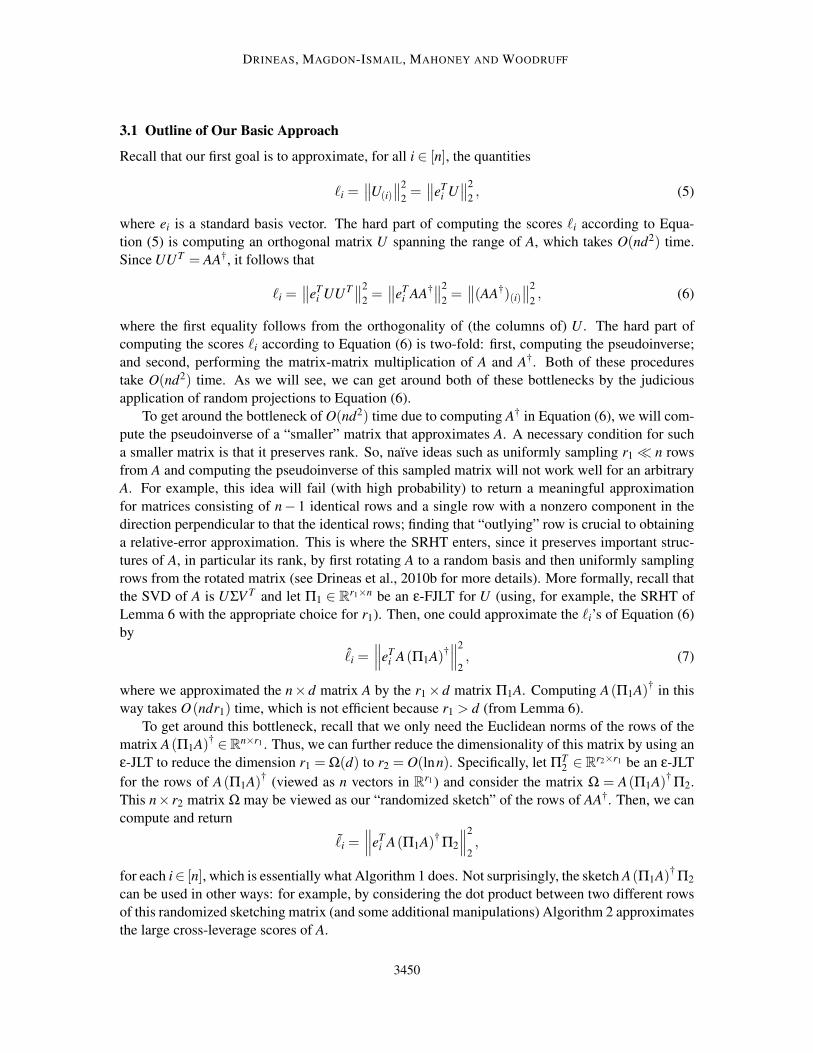
3.1 Outline of Our Basic Approach
Recall that our first goal is to approximate, for all i ∈ [n], the quantities
ℓi =∥
∥U(i)
∥
∥
2
2=∥
∥eTi U∥
∥
2
2, (5)
where ei is a standard basis vector. The hard part of computing the scores ℓi according to Equa-
tion (5) is computing an orthogonal matrix U spanning the range of A, which takes O(nd2) time.
Since UUT = AA†, it follows that
ℓi =∥
∥eTi UUT
∥
∥
2
2=∥
∥eTi AA†
∥
∥
2
2=∥
∥(AA†)(i)∥
∥
2
2, (6)
where the first equality follows from the orthogonality of (the columns of) U . The hard part of
computing the scores ℓi according to Equation (6) is two-fold: first, computing the pseudoinverse;
and second, performing the matrix-matrix multiplication of A and A†. Both of these procedures
take O(nd2) time. As we will see, we can get around both of these bottlenecks by the judicious
application of random projections to Equation (6).
To get around the bottleneck of O(nd2) time due to computing A† in Equation (6), we will com-
pute the pseudoinverse of a “smaller” matrix that approximates A. A necessary condition for such
a smaller matrix is that it preserves rank. So, naıve ideas such as uniformly sampling r1≪ n rows
from A and computing the pseudoinverse of this sampled matrix will not work well for an arbitrary
A. For example, this idea will fail (with high probability) to return a meaningful approximation
for matrices consisting of n− 1 identical rows and a single row with a nonzero component in the
direction perpendicular to that the identical rows; finding that “outlying” row is crucial to obtaining
a relative-error approximation. This is where the SRHT enters, since it preserves important struc-
tures of A, in particular its rank, by first rotating A to a random basis and then uniformly sampling
rows from the rotated matrix (see Drineas et al., 2010b for more details). More formally, recall that
the SVD of A is UΣV T and let Π1 ∈ Rr1×n be an ε-FJLT for U (using, for example, the SRHT of
Lemma 6 with the appropriate choice for r1). Then, one could approximate the ℓi’s of Equation (6)
by
ℓi =∥
∥
∥eT
i A(Π1A)†∥
∥
∥
2
2, (7)
where we approximated the n×d matrix A by the r1×d matrix Π1A. Computing A(Π1A)†in this
way takes O(ndr1) time, which is not efficient because r1 > d (from Lemma 6).
To get around this bottleneck, recall that we only need the Euclidean norms of the rows of the
matrix A(Π1A)† ∈Rn×r1 . Thus, we can further reduce the dimensionality of this matrix by using an
ε-JLT to reduce the dimension r1 = Ω(d) to r2 = O(lnn). Specifically, let ΠT2 ∈ R
r2×r1 be an ε-JLT
for the rows of A(Π1A)†(viewed as n vectors in R
r1) and consider the matrix Ω = A(Π1A)† Π2.
This n× r2 matrix Ω may be viewed as our “randomized sketch” of the rows of AA†. Then, we can
compute and return
ℓi =∥
∥
∥eT
i A(Π1A)† Π2
∥
∥
∥
2
2,
for each i∈ [n], which is essentially what Algorithm 1 does. Not surprisingly, the sketch A(Π1A)† Π2
can be used in other ways: for example, by considering the dot product between two different rows
of this randomized sketching matrix (and some additional manipulations) Algorithm 2 approximates
the large cross-leverage scores of A.
3450
FAST APPROXIMATION OF MATRIX COHERENCE AND STATISTICAL LEVERAGE
Input: A ∈ Rn×d (with SVD A =UΣV T ), error parameter ε ∈ (0,1/2].
Output: ℓi, i ∈ [n].
1. Let Π1 ∈ Rr1×n be an ε-FJLT for U , using Lemma 6 with
r1 = Ω
(
d lnn
ε2ln
(
d lnn
ε2
))
.
2. Compute Π1A ∈ Rr1×d and its SVD, Π1A =UΠ1AΣΠ1AV T
Π1A. Let
R−1 =VΠ1AΣ−1Π1A ∈ R
d×d .
(Alternatively, R could be computed by a QR factorization of Π1A.)
3. View the normalized rows of AR−1 ∈ Rn×d as n vectors in R
d , and construct
Π2 ∈ Rd×r2 to be an ε-JLT for n2 vectors (the aforementioned n vectors and their
n2−n pairwise sums), using Lemma 4 with
r2 = O(
ε−2 lnn)
.
4. Construct the matrix product Ω = AR−1Π2.
5. For all i ∈ [n] compute and return ℓi =∥
∥Ω(i)
∥
∥
2
2.
Algorithm 1: Approximating the (diagonal) statistical leverage scores ℓi.
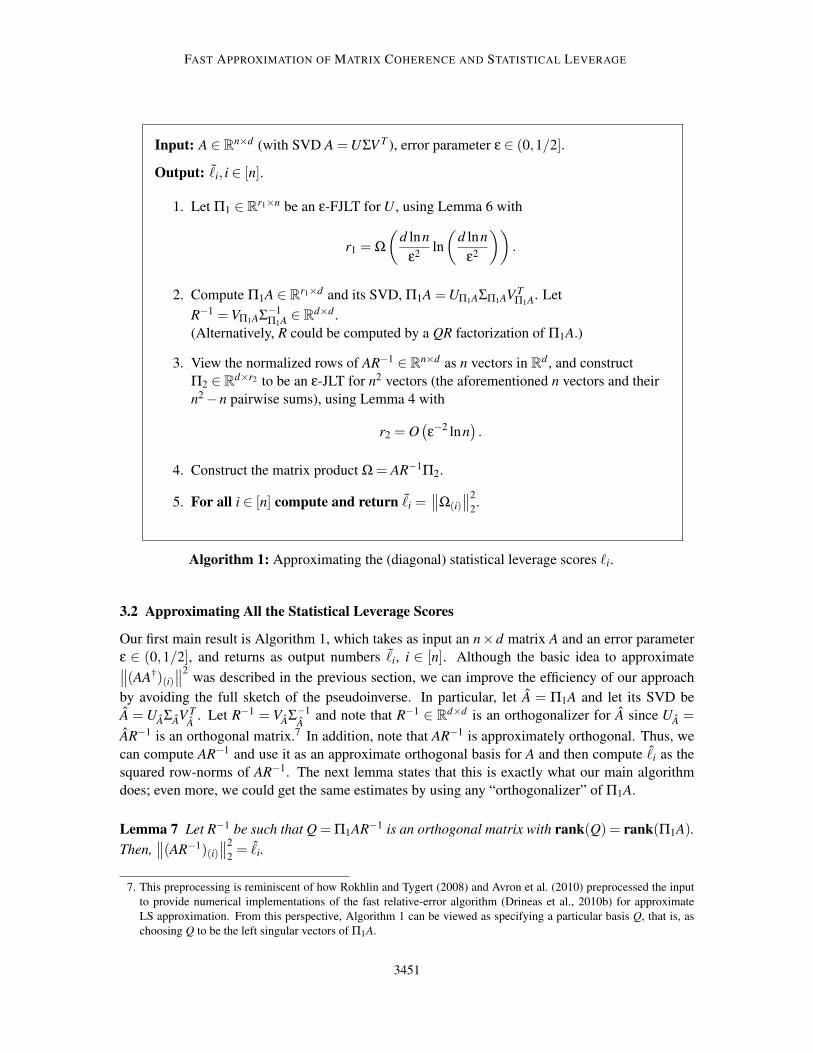
3.2 Approximating All the Statistical Leverage Scores
Our first main result is Algorithm 1, which takes as input an n×d matrix A and an error parameter
ε ∈ (0,1/2], and returns as output numbers ℓi, i ∈ [n]. Although the basic idea to approximate∥
∥(AA†)(i)∥
∥
2was described in the previous section, we can improve the efficiency of our approach
by avoiding the full sketch of the pseudoinverse. In particular, let A = Π1A and let its SVD be
A = UAΣAV TA
. Let R−1 = VAΣ−1
Aand note that R−1 ∈ R
d×d is an orthogonalizer for A since UA =
AR−1 is an orthogonal matrix.7 In addition, note that AR−1 is approximately orthogonal. Thus, we
can compute AR−1 and use it as an approximate orthogonal basis for A and then compute ℓi as the
squared row-norms of AR−1. The next lemma states that this is exactly what our main algorithm
does; even more, we could get the same estimates by using any “orthogonalizer” of Π1A.
Lemma 7 Let R−1 be such that Q = Π1AR−1 is an orthogonal matrix with rank(Q) = rank(Π1A).
Then,∥
∥(AR−1)(i)∥
∥
2
2= ℓi.
7. This preprocessing is reminiscent of how Rokhlin and Tygert (2008) and Avron et al. (2010) preprocessed the input
to provide numerical implementations of the fast relative-error algorithm (Drineas et al., 2010b) for approximate
LS approximation. From this perspective, Algorithm 1 can be viewed as specifying a particular basis Q, that is, as
choosing Q to be the left singular vectors of Π1A.
3451

DRINEAS, MAGDON-ISMAIL, MAHONEY AND WOODRUFF
Proof Since A=Π1A has rank d (by Lemma 5) and R−1 preserves this rank, R−1 is a d×d invertible
matrix. Using A = QR and properties of the pseudoinverse, we get(
A)†
= R−1QT . Thus,
ℓi =∥
∥
∥(A(Π1A)†)(i)
∥
∥
∥
2
2=∥
∥
∥
(
AR−1QT)
(i)
∥
∥
∥
2
2=∥
∥
∥
(
AR−1)
(i)QT∥
∥
∥
2
2=∥
∥
∥
(
AR−1)
(i)
∥
∥
∥
2
2.
This lemma says that the ℓi of Equation (7) can be computed with any QR decomposition, rather
than with the SVD; but note that one would still have to post-multiply by Π2, as in Algorithm 1, in
order to compute “quickly” the approximations of the leverage scores.
3.3 Approximating the Large Cross-leverage Scores
By combining Lemmas 9 and 10 (in Section 4.2 below) with the triangle inequality, one immediately
obtains the following lemma.
Lemma 8 Let Ω be either the sketching matrix constructed by Algorithm 1, that is, Ω = AR−1Π2,
or Ω = A(Π1A)† Π2 as described in Section 3.1. Then, the pairwise dot-products of the rows of Ω
are additive-error approximations to the leverage scores and cross-leverage scores:
∣
∣〈U(i),U( j)〉−〈Ω(i),Ω( j)〉∣
∣≤ 3ε
1− ε
∥
∥U(i)
∥
∥
2
∥
∥U( j)
∥
∥
2.
That is, if one were interested in obtaining an approximation to all the cross-leverage scores to
within additive error (and thus the diagonal statistical leverage scores to relative-error), then the
algorithm which first computes Ω followed by all the pairwise inner products achieves this in time
T (Ω)+O(
n2r2
)
, where T (Ω) is the time to compute Ω from Section 3.2 and r2 = O(ε−2 lnn).8 The
challenge is to avoid the n2 computational complexity and this can be done if one is interested only
in the large cross-leverage scores.
Our second main result is provided by Algorithms 2 and 3. Algorithm 2 takes as input an n×d
matrix A, a parameter κ > 1, and an error parameter ε ∈ (0,1/2], and returns as output a subset
of [n]× [n] and estimates ci j satisfying Theorem 3. The first step of the algorithm is to compute
the matrix Ω = AR−1Π2 constructed by Algorithm 1. Then, Algorithm 2 uses Algorithm 3 as a
subroutine to compute “heavy hitter” pairs of rows from a matrix.
4. Proofs of Our Main Theorems
We will start with a sketch of the proofs of Theorems 2 and 3, and then we will provide the details.
4.1 Sketch of the Proof of Theorems 2 and 3
We will start by providing a sketch of the proof of Theorems 2 and 3. A detailed proof is provided
in the next two subsections. In our analysis, we will condition on the events that Π1 ∈ Rr1×n is
an ε-FJLT for U and Π2 ∈ Rr1×r2 is an ε-JLT for n2 points in R
r1 . Note that by setting δ = 0.1 in
Lemma 4, both events hold with probability at least 0.8, which is equal to the success probability of
Theorems 2 and 3. The algorithm estimates ℓi = ‖ui‖22, where ui = eT
i A(Π1A)†Π2. First, observe
8. The exact algorithm which computes a basis first and then the pairwise inner products requires O(nd2 + n2d) time.
Thus, by using the sketch, we can already improve on this running time by a factor of d/ lnn.
3452

FAST APPROXIMATION OF MATRIX COHERENCE AND STATISTICAL LEVERAGE
Input: A ∈ Rn×d and parameters κ > 1, ε ∈ (0,1/2].
Output: The set H consisting of pairs (i, j) together with estimates ci j satisfying
Theorem 3.
1. Compute the n× r2 matrix Ω = AR−1Π2 from Algorithm 1.
2. Use Algorithm 3 with inputs Ω and κ′ = κ(1+30dε) to obtain the set H
containing all the κ′-heavy pairs of Ω.
3. Return the pairs in H as the κ-heavy pairs of A.
Algorithm 2: Approximating the large (off-diagonal) cross-leverage scores ci j.
Input: X ∈ Rn×r with rows x1, . . . ,xn and a parameter κ > 1.
Output: H = (i, j), ci j containing all heavy (unordered) pairs. The pair (i, j), ci j ∈H
if and only if c2i j = 〈xi,x j〉2 ≥
∥
∥XT X∥
∥
2
F/κ.
1: Compute the norms ‖xi‖2 and sort the rows according to norm, so that
‖x1‖2 ≤ ·· · ≤ ‖xn‖2.
2: H ←; z1← n; z2← 1.
3: while z2 ≤ z1 do
4: while ‖xz1‖2
2‖xz2‖2
2 <∥
∥XT X∥
∥
2
F/κ do
5: z2← z2 +1.
6: if z2 > z1 then
7: return H .
8: end if
9: end while
10: for each pair (i, j) where i = z1 and j ∈ z2,z2 +1, . . . ,z1 do
11: c2i j = 〈xi,x j〉2.
12: if c2i j ≥
∥
∥XT X∥
∥
2
F/κ then
13: add (i, j) and ci j to H .
14: end if
15: z1← z1−1.
16: end for
17: end while
18: return H .
Algorithm 3: Computing heavy pairs of a matrix.
that the sole purpose of Π2 is to improve the running time while preserving pairwise inner products;
3453
DRINEAS, MAGDON-ISMAIL, MAHONEY AND WOODRUFF
this is achieved because Π2 is an ε-JLT for n2 points. So, the results will follow if
eTi A(Π1A)†((Π1A)†)T AT e j ≈ eT
i UUT e j
and (Π1A)† can be computed efficiently. Since Π1 is an ε-FJLT for U , where A = UΣV T , (Π1A)†
can be computed in O(nd lnr1 + r1d2) time. By Lemma 5, (Π1A)† =V Σ−1(Π1U)†, and so
eTi A(Π1A)†((Π1A)†)T AT e j = eT
i U(Π1U)†(Π1U)†TUT e j.
Since Π1 is an ε-FJLT for U , it follows that (Π1U)†(Π1U)†T ≈ Id , that is, that Π1U is approximately
orthogonal. Theorem 2 follows from this basic idea. However, in order to prove Theorem 3, having
a sketch which preserves inner products alone is not sufficient. We also need a fast algorithm to
identify the large inner products and to relate these to the actual cross-leverage scores. Indeed, it is
possible to efficiently find pairs of rows in a general matrix with large inner products. Combining
this with the fact that the inner products are preserved, we obtain Theorem 3.
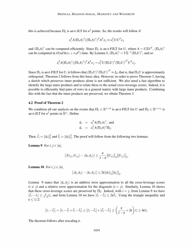
4.2 Proof of Theorem 2
We condition all our analysis on the events that Π1 ∈ Rr1×n is an ε-FJLT for U and Π2 ∈ R
r1×r2 is
an ε-JLT for n2 points in Rr1 . Define
ui = eTi A(Π1A)†, and
ui = eTi A(Π1A)†Π2.
Then, ℓi = ‖ui‖22 and ℓi = ‖ui‖2
2. The proof will follow from the following two lemmas.
Lemma 9 For i, j ∈ [n],
∣
∣〈U(i),U( j)〉−〈ui, u j〉∣
∣≤ ε
1− ε
∥
∥U(i)
∥
∥
2
∥
∥U( j)
∥
∥
2.
Lemma 10 For i, j ∈ [n],∣
∣〈ui, u j〉−〈ui, u j〉∣
∣≤ 2ε‖ui‖2
∥
∥u j
∥
∥
2.
Lemma 9 states that 〈ui, u j〉 is an additive error approximation to all the cross-leverage scores
(i 6= j) and a relative error approximation for the diagonals (i = j). Similarly, Lemma 10 shows
that these cross-leverage scores are preserved by Π2. Indeed, with i = j, from Lemma 9 we have
|ℓi− ℓi| ≤ ε1−εℓi, and from Lemma 10 we have |ℓi− ℓi| ≤ 2εℓi. Using the triangle inequality and
ε≤ 1/2:
∣
∣ℓi− ℓi
∣
∣=∣
∣ℓi− ℓi + ℓi− ℓi
∣
∣≤∣
∣ℓi− ℓi
∣
∣+∣
∣ℓi− ℓi
∣
∣≤(
ε
1− ε+2ε
)
ℓi ≤ 4εℓi.
The theorem follows after rescaling ε.
3454

FAST APPROXIMATION OF MATRIX COHERENCE AND STATISTICAL LEVERAGE
Proof of Lemma 9 Let A =UΣV T . Using this SVD of A and Equation (4) in Lemma 5,
〈ui, u j〉 = eTi UΣV TV Σ−1 (Π1U)† (Π1U)†T
Σ−1V TV ΣUT e j = eTi U (Π1U)† (Π1U)†T
UT e j.
By performing standard manipulations, we can now bound∣
∣〈U(i),U( j)〉−〈ui, u j〉∣
∣:
∣
∣〈U(i),U( j)〉−〈ui, u j〉∣
∣ = eTi UUT e j− eT
i U (Π1U)† (Π1U)†TUT e j
= eTi U(
Id− (Π1U)† (Π1U)†T)
UT e j
≤∥
∥
∥Id− (Π1U)† (Π1U)†T
∥
∥
∥
2
∥
∥U(i)
∥
∥
2
∥
∥U( j)
∥
∥
2.
Let the SVD of Ψ = Π1U be Ψ = UΨΣΨV TΨ , where VΨ is a full rotation in d dimensions (because
rank(A) = rank(Π1U)). Then, Ψ†Ψ†T=VΨΣ−2
Ψ V TΨ . Thus,
∣
∣〈U(i),U( j)〉−〈ui, u j〉∣
∣ ≤∥
∥Id−VΨΣ−2Ψ V T
Ψ
∥
∥
2
∥
∥U(i)
∥
∥
2
∥
∥U( j)
∥
∥
2
=∥
∥VΨV TΨ −VΨΣ−2
Ψ V TΨ
∥
∥
2
∥
∥U(i)
∥
∥
2
∥
∥U( j)
∥
∥
2
=∥
∥Id−Σ−2Ψ
∥
∥
2
∥
∥U(i)
∥
∥
2
∥
∥U( j)
∥
∥
2,
where we used the fact that VΨV TΨ = V T
ΨVΨ = Id and the unitary invariance of the spectral norm.
Finally, using Equation (3) of Lemma 5 the result follows.
Proof of Lemma 10. Since Π2 is an ε-JLT for n2 vectors, it preserves the norms of an arbitrary
(but fixed) collection of n2 vectors. Let xi = ui/‖ui‖2. Consider the following n2 vectors:
xi for i ∈ [n], and
xi + x j for i, j ∈ [n], i 6= j.
By the ε-JLT property of Π2 and the fact that ‖xi‖2 = 1,
1− ε≤ ‖xiΠ2‖22 ≤ 1+ ε for i ∈ [n], and (8)
(1− ε)∥
∥xi + x j
∥
∥
2
2≤∥
∥xiΠ2 + x jΠ2
∥
∥
2
2≤ (1+ ε)
∥
∥xi + x j
∥
∥
2
2for i, j ∈ [n], i 6= j. (9)
Combining Equations (8) and (9) after expanding the squares using the identity ‖a+b‖2 = ‖a‖2 +‖b‖2 +2〈a,b〉, substituting ‖xi‖= 1, and after some algebra, we obtain
〈xi,x j〉−2ε≤ 〈xiΠ2,x jΠ2〉 ≤ 〈xi,x j〉+2ε.
To conclude the proof, multiply throughout by ‖ui‖∥
∥u j
∥
∥ and use the homogeneity of the inner
product, together with the linearity of Π2, to obtain:
〈ui, u j〉−2ε‖ui‖∥
∥u j
∥
∥≤ 〈uiΠ2, u jΠ2〉 ≤ 〈ui, u j〉+2ε‖ui‖∥
∥u j
∥
∥.
Running Times. By Lemma 7, we can use VΠ1AΣ−1Π1A instead of (Π1A)† and obtain the same
estimates. Since Π1 is an ε-FJLT, the product Π1A can be computed in O(nd lnr1) while its
SVD takes an additional O(r1d2) time to return VΠ1AΣ−1Π1A ∈ R
d×d . Since Π2 ∈ Rd×r2 , we obtain
VΠ1AΣ−1Π1AΠ2 ∈ R
d×r2 in an additional O(r2d2) time. Finally, premultiplying by A takes O(ndr2)
3455
DRINEAS, MAGDON-ISMAIL, MAHONEY AND WOODRUFF
time, and computing and returning the squared row-norms of Ω = AVΠ1AΣ−1Π1AΠ2 ∈ R
n×r2 takes
O(nr2) time. So, the total running time is the sum of all these operations, which is
O(nd lnr1 +ndr2 + r1d2 + r2d2).
Recall that for our implementations of the ε-JLTs and ε-FJLTs, we have δ = 0.1, and we have
r1 = O(
ε−2d (lnn)(
ln(
ε−2d lnn)))
and r2 = O(ε−2 lnn). It follows that the asymptotic running
time is
O(
nd ln(
dε−1)
+ndε−2 lnn+d3ε−2 (lnn)(
ln(
dε−1)))
.
To simplify, suppose that d ≤ n≤ ed and treat ε as a constant. Then, the asymptotic running time is
O(
nd lnn+d3 (lnn)(lnd))
.
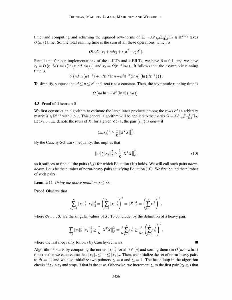
4.3 Proof of Theorem 3
We first construct an algorithm to estimate the large inner products among the rows of an arbitrary
matrix X ∈Rn×r with n> r. This general algorithm will be applied to the matrix Ω= AVΠ1AΣ−1Π1AΠ2.
Let x1, . . . ,xn denote the rows of X ; for a given κ > 1, the pair (i, j) is heavy if
〈xi,x j〉2 ≥1
κ
∥
∥XT X∥
∥
2
F.
By the Cauchy-Schwarz inequality, this implies that
‖xi‖22
∥
∥x j
∥
∥
2
2≥ 1
κ
∥
∥XT X∥
∥
2
F, (10)
so it suffices to find all the pairs (i, j) for which Equation (10) holds. We will call such pairs norm-
heavy. Let s be the number of norm-heavy pairs satisfying Equation (10). We first bound the number
of such pairs.
Lemma 11 Using the above notation, s≤ κr.
Proof Observe that
n
∑i, j=1
‖xi‖22
∥
∥x j
∥
∥
2
2=
(
n
∑i=1
‖xi‖22
)2
= ‖X‖4F =
(
r
∑i=1
σ2i
)2
,
where σ1, . . . ,σr are the singular values of X . To conclude, by the definition of a heavy pair,
∑i, j
‖xi‖22
∥
∥x j
∥
∥
2
2≥ s
κ
∥
∥XT X∥
∥
2
F=
s
κ
r
∑i=1
σ4i ≥
s
κr
(
r
∑i=1
σ2i
)2
,
where the last inequality follows by Cauchy-Schwarz.
Algorithm 3 starts by computing the norms ‖xi‖22 for all i ∈ [n] and sorting them (in O(nr+n lnn)
time) so that we can assume that ‖x1‖2≤ ·· · ≤ ‖xn‖2. Then, we initialize the set of norm-heavy pairs
to H = and we also initialize two pointers z1 = n and z2 = 1. The basic loop in the algorithm
checks if z2 > z1 and stops if that is the case. Otherwise, we increment z2 to the first pair (z1,z2) that
3456
FAST APPROXIMATION OF MATRIX COHERENCE AND STATISTICAL LEVERAGE
is norm-heavy. If none of pairs are norm heavy (i.e., z2 > z1 occurs), then we stop and output H ;
otherwise, we add (z1,z2),(z1,z2 + 1), . . . ,(z1,z1) to H . This basic loop computes all pairs (z1, i)with i ≤ z1 that are norm-heavy. Next, we decrease z1 by one and if z1 < z2 we stop and output
H ; otherwise, we repeat the basic loop. Note that in the basic loop z2 is always incremented. This
occurs whenever the pair (z1,z2) is not norm-heavy. Since z2 can be incremented at most n times,
the number of times we check whether a pair is norm-heavy and fail is at most n. Every successful
check results in the addition of at least one norm-heavy pair into H and thus the number of times
we check if a pair is norm heavy (a constant-time operation) is at most n+ s. The number of pair
additions into H is exactly s and thus the total running time is O(nr+n lnn+ s). Finally, we must
check each norm-heavy pair to verify whether or not it is actually heavy by computing s inner
products vectors in Rr; this can be done in O(sr) time. Using s≤ κr we get the following lemma.
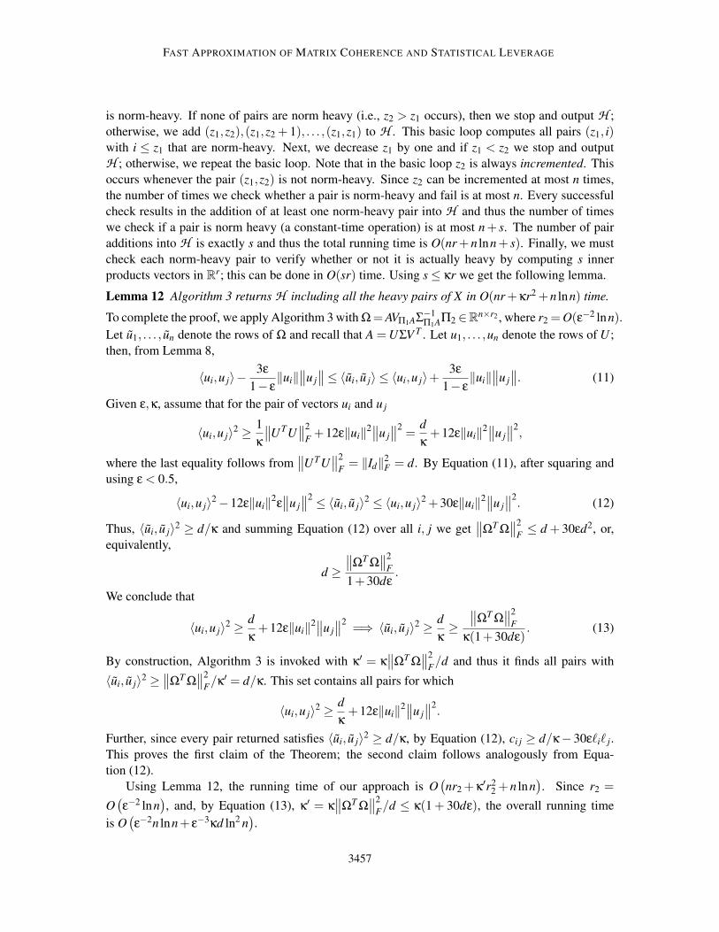
Lemma 12 Algorithm 3 returns H including all the heavy pairs of X in O(nr+κr2 +n lnn) time.
To complete the proof, we apply Algorithm 3 with Ω=AVΠ1AΣ−1Π1AΠ2 ∈Rn×r2 , where r2 =O(ε−2 lnn).
Let u1, . . . , un denote the rows of Ω and recall that A =UΣV T . Let u1, . . . ,un denote the rows of U ;
then, from Lemma 8,
〈ui,u j〉−3ε
1− ε‖ui‖
∥
∥u j
∥
∥≤ 〈ui, u j〉 ≤ 〈ui,u j〉+3ε
1− ε‖ui‖
∥
∥u j
∥
∥. (11)
Given ε,κ, assume that for the pair of vectors ui and u j
〈ui,u j〉2 ≥1
κ
∥
∥UTU∥
∥
2
F+12ε‖ui‖2
∥
∥u j
∥
∥
2=
d
κ+12ε‖ui‖2
∥
∥u j
∥
∥
2,
where the last equality follows from∥
∥UTU∥
∥
2
F= ‖Id‖2
F = d. By Equation (11), after squaring and
using ε < 0.5,
〈ui,u j〉2−12ε‖ui‖2ε∥
∥u j
∥
∥
2 ≤ 〈ui, u j〉2 ≤ 〈ui,u j〉2 +30ε‖ui‖2∥
∥u j
∥
∥
2. (12)
Thus, 〈ui, u j〉2 ≥ d/κ and summing Equation (12) over all i, j we get∥
∥ΩT Ω∥
∥
2
F≤ d + 30εd2, or,
equivalently,
d ≥∥
∥ΩT Ω∥
∥
2
F
1+30dε.
We conclude that
〈ui,u j〉2 ≥d
κ+12ε‖ui‖2
∥
∥u j
∥
∥
2=⇒ 〈ui, u j〉2 ≥
d
κ≥
∥
∥ΩT Ω∥
∥
2
F
κ(1+30dε). (13)
By construction, Algorithm 3 is invoked with κ′ = κ∥
∥ΩT Ω∥
∥
2
F/d and thus it finds all pairs with
〈ui, u j〉2 ≥∥
∥ΩT Ω∥
∥
2
F/κ′ = d/κ. This set contains all pairs for which
〈ui,u j〉2 ≥d
κ+12ε‖ui‖2
∥
∥u j
∥
∥
2.
Further, since every pair returned satisfies 〈ui, u j〉2 ≥ d/κ, by Equation (12), ci j ≥ d/κ− 30εℓiℓ j.
This proves the first claim of the Theorem; the second claim follows analogously from Equa-
tion (12).
Using Lemma 12, the running time of our approach is O(
nr2 +κ′r22 +n lnn
)
. Since r2 =
O(
ε−2 lnn)
, and, by Equation (13), κ′ = κ∥
∥ΩT Ω∥
∥
2
F/d ≤ κ(1+ 30dε), the overall running time
is O(
ε−2n lnn+ ε−3κd ln2 n)
.
3457
DRINEAS, MAGDON-ISMAIL, MAHONEY AND WOODRUFF
5. Extending Our Algorithm to General Matrices
In this section, we will describe an important extension of our main result, namely the computation
of the statistical leverage scores relative to the best rank-k approximation to a general matrix A. More
specifically, we consider the estimation of leverage scores for the case of general “fat” matrices,
namely input matrices A∈Rn×d , where both n and d are large, for example, when d = n or d =Θ(n).Clearly, the leverage scores of any full rank n×n matrix are exactly uniform. The problem becomes
interesting if one specifies a rank parameter k≪minn,d. This may arise when the numerical rank
of A is small (e.g., in some scientific computing applications, more than 99% of the spectral norm of
A may be captured by some k≪minn,d directions), or, more generally, when one is interested in
some low rank approximation to A (e.g., in some data analysis applications, a reasonable fraction or
even the majority of the Frobenius norm of A may be captured by some k≪ minn,d directions,
where k is determined by some exogenously-specified model selection criterion). Thus, assume that
in addition to a general n× d matrix A, a rank parameter k < minn,d is specified. In this case,
we wish to obtain the statistical leverage scores ℓi =∥
∥(Uk)(i)∥
∥
2
2for Ak = UkΣkV
Tk , the best rank-k
approximation to A. Equivalently, we seek the normalized leverage scores
pi =ℓi
k. (14)
Note that ∑ni=1 pi = 1 since ∑n
i=1 ℓi = ‖Uk‖2F = k.
Unfortunately, as stated, this is an ill-posed problem. Indeed, consider the degenerate case when
A = In (i.e., the n×n identity matrix). In this case, Uk is not unique and the leverage scores are not
well-defined. Moreover, for the obvious(
nk
)
equivalent choices for Uk, the leverage scores defined
according to any one of these choices do not provide a relative error approximation to the leverage
scores defined according to any other choices. More generally, removing this trivial degeneracy
does not help. Consider the matrix
A =
(
Ik 0
0 (1− γ)In−k
)
∈ Rn×n.
In this example, the leverage scores for Ak are well defined. However, as γ→ 0, it is not possible
to distinguish between the top-k singular space and its complement. This example suggests that it
should be possible to obtain some result conditioning on the spectral gap at the kth singular value.
For example, one might assume that σ2k −σ2
k+1 ≥ γ > 0, in which case the parameter γ would play
an important role in the ability to solve this problem. Any algorithm which cannot distinguish the
singular values with an error less than γ will confuse the k-th and (k+ 1)-th singular vectors and
consequently will fail to get an accurate approximation to the leverage scores for Ak.
In the following, we take a more natural approach which leads to a clean problem formulation.
To do so, recall that the leverage scores and the related normalized leverage scores of Equation (14)
are used to approximate the matrix in some way, for example, we might be seeking a low-rank ap-
proximation to the matrix with respect to the spectral (Drineas et al., 2008) or the Frobenius (Bout-
sidis et al., 2009) norm, or we might be seeking useful features or data points in downstream data
analysis applications (Paschou et al., 2007; Mahoney and Drineas, 2009), or we might be seeking
to develop high-quality numerical implementations of low-rank matrix approximation algorithms
(Halko et al., 2011), etc. In all these cases, we only care that the estimated leverage scores are
a good approximation to the leverage scores of some “good” low-rank approximation to A. The
3458

FAST APPROXIMATION OF MATRIX COHERENCE AND STATISTICAL LEVERAGE
following definition captures the notion of a set of rank-k matrices that are good approximations to
A.
Definition 13 Given A ∈ Rn×d and a rank parameter k ≪ minn,d, let Ak be the best rank-k
approximation to A. Define the set Sε of rank-k matrices that are good approximations to A as
follows (for ξ = 2,F):
Sε =
X ∈ Rn×d : rank(X) = k and ‖A−X‖ξ ≤ (1+ ε)‖A−Ak‖ξ
.
We are now ready to define our approximations to the normalized leverage scores of any matrix
A ∈Rn×d given a rank parameter k≪minn,d. Instead of seeking to approximate the pi of Equa-
tion (14) (a problem that is ill-posed as discussed above), we will be satisfied if we can approximate
the normalized leverage scores of some matrix X ∈ Sε. This is an interesting relaxation of the task
at hand: all matrices X that are sufficiently close to Ak are essentially equivalent, since they can be
used instead of Ak in applications.
Definition 14 Given A∈Rn×d and a rank parameter k≪minn,d, let Sε be the set of matrices of
Definition 13. We call the numbers pi (for all i ∈ [n]) β-approximations to the normalized leverage
scores of Ak (the best rank-k approximation to A) if, for some matrix X ∈ Sε,
pi ≥β∥
∥(UX)(i)∥
∥
2
2
kand
n
∑i=1
pi = 1.
Here UX ∈ Rn×k is the matrix of the left singular vectors of X.
Thus, we will seek algorithms whose output is a set of numbers, with the requirement that those
numbers are good approximations to the normalized leverage scores of some matrix X ∈ Sε (instead
of Ak). This removes the ill-posedness of the original problem. Next, we will give two examples
of algorithms that compute such β-approximations to the normalized leverage scores of a general
matrix A with a rank parameter k for two popular norms, the spectral norm and the Frobenius norm.9
5.1 Leverage Scores for Spectral Norm Approximators
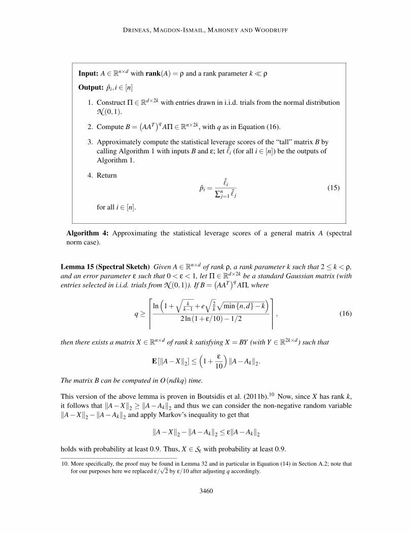
Algorithm 4 approximates the statistical leverage scores of a general matrix A with rank parameter
k in the spectral norm case. It takes as inputs a matrix A ∈Rn×d with rank(A) = ρ and a rank
parameter k≪ ρ, and outputs a set of numbers pi for all i ∈ [n], namely our approximations to the
normalized leverage scores of A with rank parameter k.The next lemma argues that there exists a matrix X ∈Rn×d of rank k that is sufficiently close to A
(in particular, it is a member of Sε with constant probability) and, additionally, can be written as X =BY, where Y ∈R2k×d is a matrix of rank k. A version of this lemma was essentially proven in Halko
et al. (2011), but see also Rokhlin et al. (2009) for computational details; we will use the version
of the lemma that appeared in Boutsidis et al. (2011b). (See also the conference version (Boutsidis
et al., 2011a), but in the remainder we refer to the technical report version (Boutsidis et al., 2011b)
for consistency of numbering.) Note that for our purposes in this section, the computation of Y is
not relevant and we defer the reader to Halko et al. (2011) and Boutsidis et al. (2011b) for details.
9. Note that we will not compute Sε, but our algorithms will compute a matrix in that set. Moreover, that matrix can be
used for high-quality low-rank matrix approximation. See the comments in Section 1.4 for more details.
3459
DRINEAS, MAGDON-ISMAIL, MAHONEY AND WOODRUFF
Input: A ∈ Rn×d with rank(A) = ρ and a rank parameter k≪ ρ
Output: pi, i ∈ [n]
1. Construct Π ∈ Rd×2k with entries drawn in i.i.d. trials from the normal distribution
N (0,1).
2. Compute B =(
AAT)q
AΠ ∈ Rn×2k, with q as in Equation (16).
3. Approximately compute the statistical leverage scores of the “tall” matrix B by
calling Algorithm 1 with inputs B and ε; let ℓi (for all i ∈ [n]) be the outputs of
Algorithm 1.
4. Return
pi =ℓi
∑nj=1 ℓ j
(15)
for all i ∈ [n].
Algorithm 4: Approximating the statistical leverage scores of a general matrix A (spectral
norm case).
Lemma 15 (Spectral Sketch) Given A ∈ Rn×d of rank ρ, a rank parameter k such that 2≤ k < ρ,
and an error parameter ε such that 0 < ε < 1, let Π ∈ Rd×2k be a standard Gaussian matrix (with
entries selected in i.i.d. trials from N (0,1)). If B =(
AAT)q
AΠ, where
q≥
ln(
1+√
kk−1
+ e
√
2k
√
minn,d− k)
2ln(1+ ε/10)−1/2
, (16)
then there exists a matrix X ∈ Rn×d of rank k satisfying X = BY (with Y ∈ R
2k×d) such that
E [‖A−X‖2]≤(
1+ε
10
)
‖A−Ak‖2.
The matrix B can be computed in O(ndkq) time.
This version of the above lemma is proven in Boutsidis et al. (2011b).10 Now, since X has rank k,
it follows that ‖A−X‖2 ≥ ‖A−Ak‖2 and thus we can consider the non-negative random variable
‖A−X‖2−‖A−Ak‖2 and apply Markov’s inequality to get that
‖A−X‖2−‖A−Ak‖2 ≤ ε‖A−Ak‖2
holds with probability at least 0.9. Thus, X ∈ Sε with probability at least 0.9.
10. More specifically, the proof may be found in Lemma 32 and in particular in Equation (14) in Section A.2; note that
for our purposes here we replaced ε/√
2 by ε/10 after adjusting q accordingly.
3460
FAST APPROXIMATION OF MATRIX COHERENCE AND STATISTICAL LEVERAGE
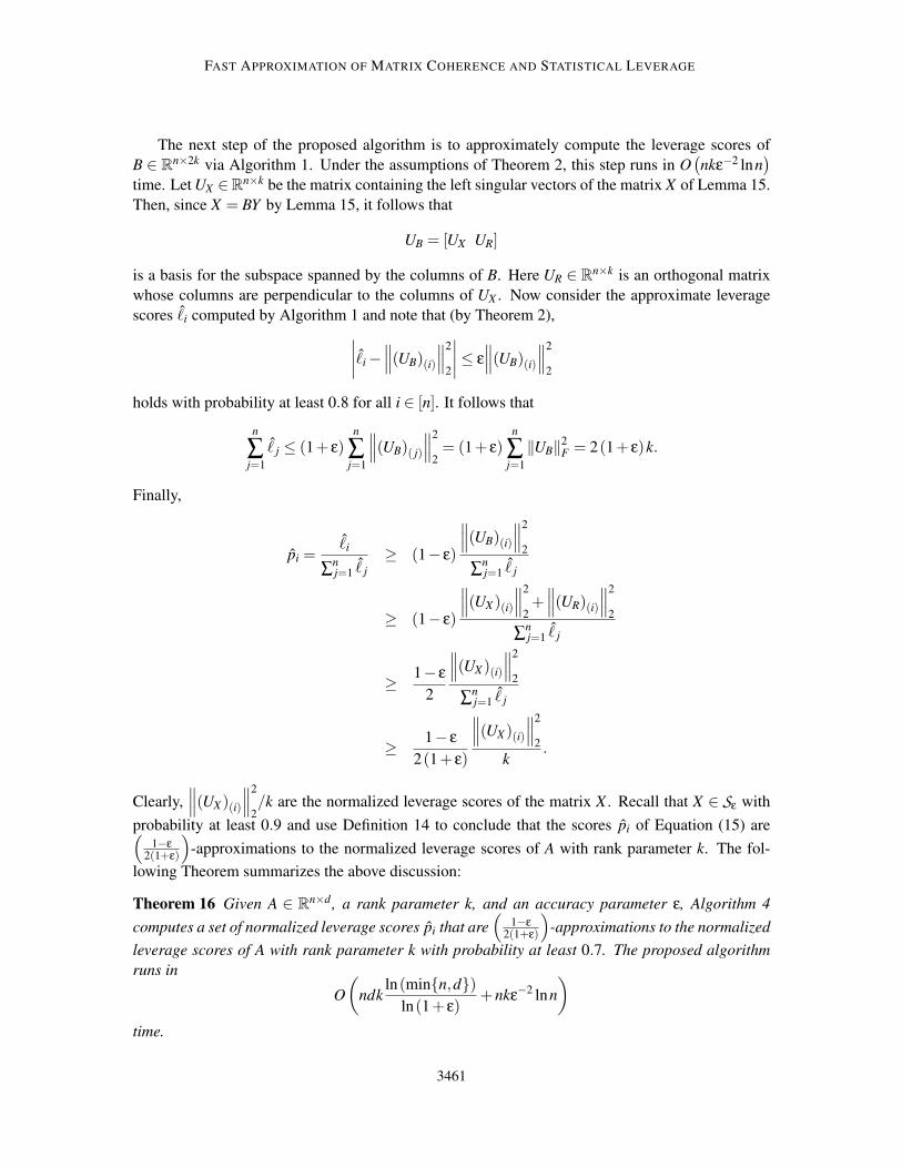
The next step of the proposed algorithm is to approximately compute the leverage scores of
B ∈ Rn×2k via Algorithm 1. Under the assumptions of Theorem 2, this step runs in O
(
nkε−2 lnn)
time. Let UX ∈Rn×k be the matrix containing the left singular vectors of the matrix X of Lemma 15.
Then, since X = BY by Lemma 15, it follows that
UB = [UX UR]
is a basis for the subspace spanned by the columns of B. Here UR ∈ Rn×k is an orthogonal matrix
whose columns are perpendicular to the columns of UX . Now consider the approximate leverage
scores ℓi computed by Algorithm 1 and note that (by Theorem 2),
∣
∣
∣
∣
ℓi−∥
∥
∥(UB)(i)
∥
∥
∥
2
2
∣
∣
∣
∣
≤ ε∥
∥
∥(UB)(i)
∥
∥
∥
2
2
holds with probability at least 0.8 for all i ∈ [n]. It follows that
n
∑j=1
ℓ j ≤ (1+ ε)n
∑j=1
∥
∥
∥(UB)( j)
∥
∥
∥
2
2= (1+ ε)
n
∑j=1
‖UB‖2F = 2(1+ ε)k.
Finally,
pi =ℓi
∑nj=1 ℓ j
≥ (1− ε)
∥
∥
∥(UB)(i)
∥
∥
∥
2
2
∑nj=1 ℓ j
≥ (1− ε)
∥
∥
∥(UX)(i)
∥
∥
∥
2
2+∥
∥
∥(UR)(i)
∥
∥
∥
2
2
∑nj=1 ℓ j
≥ 1− ε
2
∥
∥
∥(UX)(i)
∥
∥
∥
2
2
∑nj=1 ℓ j
≥ 1− ε
2(1+ ε)
∥
∥
∥(UX)(i)
∥
∥
∥
2
2
k.
Clearly,
∥
∥
∥(UX)(i)
∥
∥
∥
2
2/k are the normalized leverage scores of the matrix X . Recall that X ∈ Sε with
probability at least 0.9 and use Definition 14 to conclude that the scores pi of Equation (15) are(
1−ε2(1+ε)
)
-approximations to the normalized leverage scores of A with rank parameter k. The fol-
lowing Theorem summarizes the above discussion:
Theorem 16 Given A ∈ Rn×d , a rank parameter k, and an accuracy parameter ε, Algorithm 4
computes a set of normalized leverage scores pi that are(
1−ε2(1+ε)
)
-approximations to the normalized
leverage scores of A with rank parameter k with probability at least 0.7. The proposed algorithm
runs in
O
(
ndkln(minn,d)
ln(1+ ε)+nkε−2 lnn
)
time.
3461

DRINEAS, MAGDON-ISMAIL, MAHONEY AND WOODRUFF
Input: A ∈ Rn×d with rank(A) = ρ and a rank parameter k≪ ρ
Output: pi, i ∈ [n]
1. Let r be as in Equation (18) and construct Π ∈ Rd×r whose entries are drawn in
i.i.d. trials from the normal distribution N (0,1).
2. Compute B = AΠ ∈ Rn×r.
3. Compute a matrix Q ∈ Rn×r whose columns form an orthonormal basis for the
column space of B.
4. Compute the matrix QT A ∈ Rr×d and its left singular vectors UQT A ∈ R
r×d .
5. Let UQT A,k ∈ Rr×k denote the top k left singular vectors of the matrix QT A (the
first k columns of UQT A) and compute, for all i ∈ [n],
ℓi =∥
∥
∥
(
QUQT A,k
)
(i)
∥
∥
∥
2
2. (17)
6. Return pi = ℓi/k for all i ∈ [n].
Algorithm 5: Approximating the statistical leverage scores of a general matrix A (Frobenius
norm case).
5.2 Leverage Scores for Frobenius Norm Approximators
Algorithm 5 approximates the statistical leverage scores of a general matrix A with rank param-
eter k in the Frobenius norm case. It takes as inputs a matrix A ∈Rn×d with rank(A) = ρ and
a rank parameter k ≪ ρ, and outputs a set of numbers pi for all i ∈ [n], namely our approxi-
mations to the normalized leverage scores of A with rank parameter k. It is worth noting that
∑ni=1 ℓi =
∥
∥QUQT A,k
∥
∥
2
F=∥
∥UQT A,k
∥
∥
2
F= k and thus the pi sum up to one. The next lemma argues that
there exists a matrix X ∈ Rn×d of rank k that is sufficiently close to A (in particular, it is a member
of Sε with constant probability). Unlike the previous section (the spectral norm case), we will now
be able to provide a closed-form formula for this matrix X and, more importantly, the normalized
leverage scores of X will be exactly equal to the pi returned by our algorithm. Thus, in the parlance
of Definition 14, we will get a 1-approximation to the normalized leverage scores of A with rank
parameter k.
Lemma 17 (Frobenius Sketch) Given A∈Rn×d of rank ρ, a rank parameter k such that 2≤ k < ρ,
and an error parameter ε such that 0 < ε < 1, let Π ∈ Rd×r be a standard Gaussian matrix (with
entries selected in i.i.d. trials from N (0,1)) with
r ≥ k+
⌈
10k
ε+1
⌉
. (18)
3462
FAST APPROXIMATION OF MATRIX COHERENCE AND STATISTICAL LEVERAGE
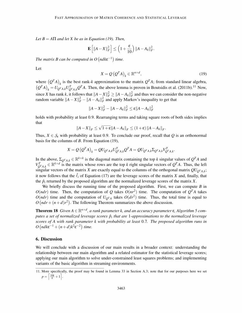
Let B = AΠ and let X be as in Equation (19). Then,
E[
‖A−X‖2F
]
≤(
1+ε
10
)
‖A−Ak‖2F .
The matrix B can be computed in O(
ndkε−1)
time.
Let
X = Q(
QT A)
k∈ R
n×d , (19)
where(
QT A)
kis the best rank-k approximation to the matrix QT A; from standard linear algebra,
(
QT A)
k=UQT A,kU
TQT A,kQT A. Then, the above lemma is proven in Boutsidis et al. (2011b).11 Now,
since X has rank k, it follows that ‖A−X‖2F ≥‖A−Ak‖2
F and thus we can consider the non-negative
random variable ‖A−X‖2F −‖A−Ak‖2
F and apply Markov’s inequality to get that
‖A−X‖2F −‖A−Ak‖2
F ≤ ε‖A−Ak‖2F
holds with probability at least 0.9. Rearranging terms and taking square roots of both sides implies
that
‖A−X‖F ≤√
1+ ε‖A−Ak‖F ≤ (1+ ε)‖A−Ak‖F .
Thus, X ∈ Sε with probability at least 0.9. To conclude our proof, recall that Q is an orthonormal
basis for the columns of B. From Equation (19),
X = Q(
QT A)
k= QUQT A,kU
TQT A,kQT A = QUQT A,kΣQT A,kV
TQT A,k.
In the above, ΣQT A,k ∈ Rk×k is the diagonal matrix containing the top k singular values of QT A and
V TQT A,k ∈ R
k×d is the matrix whose rows are the top k right singular vectors of QT A. Thus, the left
singular vectors of the matrix X are exactly equal to the columns of the orthogonal matrix QUQT A,k;
it now follows that the ℓi of Equation (17) are the leverage scores of the matrix X and, finally, that
the pi returned by the proposed algorithm are the normalized leverage scores of the matrix X .
We briefly discuss the running time of the proposed algorithm. First, we can compute B in
O(ndr) time. Then, the computation of Q takes O(nr2) time. The computation of QT A takes
O(ndr) time and the computation of UQT A takes O(dr2) time. Thus, the total time is equal to
O(
ndr+(n+d)r2)
. The following Theorem summarizes the above discussion.
Theorem 18 Given A∈Rn×d , a rank parameter k, and an accuracy parameter ε, Algorithm 5 com-
putes a set of normalized leverage scores pi that are 1-approximations to the normalized leverage
scores of A with rank parameter k with probability at least 0.7. The proposed algorithm runs in
O(
ndkε−1 +(n+d)k2ε−2)
time.
6. Discussion
We will conclude with a discussion of our main results in a broader context: understanding the
relationship between our main algorithm and a related estimator for the statistical leverage scores;
applying our main algorithm to solve under-constrained least squares problems; and implementing
variants of the basic algorithm in streaming environments.
11. More specifically, the proof may be found in Lemma 33 in Section A.3; note that for our purposes here we set
p =⌈
10kε +1
⌉
.
3463
DRINEAS, MAGDON-ISMAIL, MAHONEY AND WOODRUFF
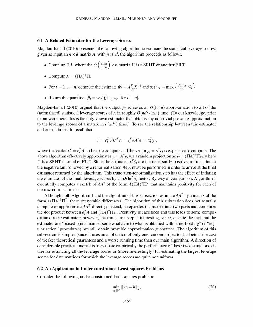
6.1 A Related Estimator for the Leverage Scores
Magdon-Ismail (2010) presented the following algorithm to estimate the statistical leverage scores:
given as input an n×d matrix A, with n≫ d, the algorithm proceeds as follows.
• Compute ΠA, where the O(
n lnd
ln2 n
)
×n matrix Π is a SRHT or another FJLT.
• Compute X = (ΠA)†Π.
• For t = 1, . . . ,n, compute the estimate wt = AT(t)X
(t) and set wt = max
d ln2 n4n
, wt
.
• Return the quantities pi = wi/∑ni′=1 wi′ , for i ∈ [n].
Magdon-Ismail (2010) argued that the output pi achieves an O(ln2 n) approximation to all of the
(normalized) statistical leverage scores of A in roughly O(nd2/ lnn) time. (To our knowledge, prior
to our work here, this is the only known estimator that obtains any nontrivial provable approximation
to the leverage scores of a matrix in o(nd2) time.) To see the relationship between this estimator
and our main result, recall that
ℓi = eTi UUT ei = eT
i AA†ei = xTi yi,
where the vector xTi = eT
i A is cheap to compute and the vector yi =A†ei is expensive to compute. The
above algorithm effectively approximates yi =A†ei via a random projection as yi =(ΠA)†Πei, where
Π is a SRHT or another FJLT. Since the estimates xTi yi are not necessarily positive, a truncation at
the negative tail, followed by a renormalization step, must be performed in order to arrive at the final
estimator returned by the algorithm. This truncation-renormalization step has the effect of inflating
the estimates of the small leverage scores by an O(ln2 n) factor. By way of comparison, Algorithm 1
essentially computes a sketch of AA† of the form A(ΠA)†ΠT that maintains positivity for each of
the row norm estimates.
Although both Algorithm 1 and the algorithm of this subsection estimate AA† by a matrix of the
form A(ΠA)†ΠT , there are notable differences. The algorithm of this subsection does not actually
compute or approximate AAT directly; instead, it separates the matrix into two parts and computes
the dot product between eTi A and (ΠA)†Πei. Positivity is sacrificed and this leads to some compli-
cations in the estimator; however, the truncation step is interesting, since, despite the fact that the
estimates are “biased” (in a manner somewhat akin to what is obtained with “thresholding” or “reg-
ularization” procedures), we still obtain provable approximation guarantees. The algorithm of this
subsection is simpler (since it uses an application of only one random projection), albeit at the cost
of weaker theoretical guarantees and a worse running time than our main algorithm. A direction of
considerable practical interest is to evaluate empirically the performance of these two estimators, ei-
ther for estimating all the leverage scores or (more interestingly) for estimating the largest leverage
scores for data matrices for which the leverage scores are quite nonuniform.
6.2 An Application to Under-constrained Least-squares Problems
Consider the following under-constrained least-squares problem:
minx∈Rd‖Ax−b‖2 , (20)
3464
FAST APPROXIMATION OF MATRIX COHERENCE AND STATISTICAL LEVERAGE
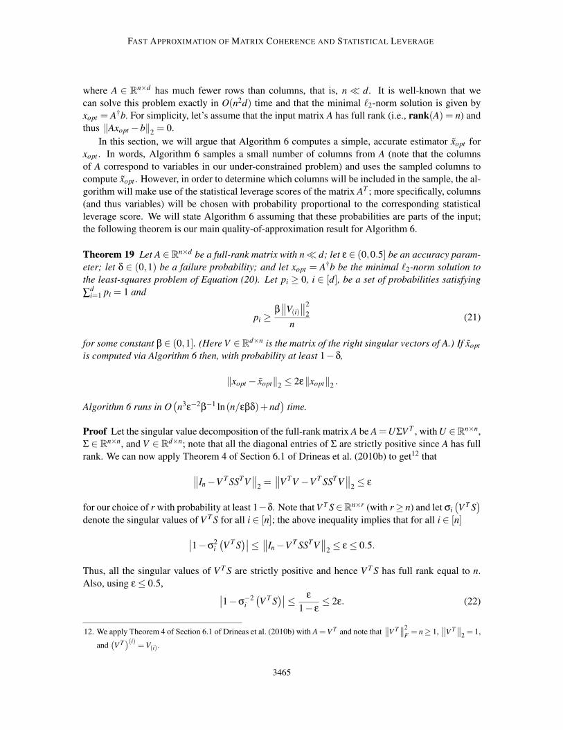
where A ∈ Rn×d has much fewer rows than columns, that is, n≪ d. It is well-known that we
can solve this problem exactly in O(n2d) time and that the minimal ℓ2-norm solution is given by
xopt = A†b. For simplicity, let’s assume that the input matrix A has full rank (i.e., rank(A) = n) and
thus ‖Axopt −b‖2= 0.
In this section, we will argue that Algorithm 6 computes a simple, accurate estimator xopt for
xopt . In words, Algorithm 6 samples a small number of columns from A (note that the columns
of A correspond to variables in our under-constrained problem) and uses the sampled columns to
compute xopt . However, in order to determine which columns will be included in the sample, the al-
gorithm will make use of the statistical leverage scores of the matrix AT ; more specifically, columns
(and thus variables) will be chosen with probability proportional to the corresponding statistical
leverage score. We will state Algorithm 6 assuming that these probabilities are parts of the input;
the following theorem is our main quality-of-approximation result for Algorithm 6.
Theorem 19 Let A ∈Rn×d be a full-rank matrix with n≪ d; let ε ∈ (0,0.5] be an accuracy param-
eter; let δ ∈ (0,1) be a failure probability; and let xopt = A†b be the minimal ℓ2-norm solution to
the least-squares problem of Equation (20). Let pi ≥ 0, i ∈ [d], be a set of probabilities satisfying
∑di=1 pi = 1 and
pi ≥β∥
∥V(i)
∥
∥
2
2
n(21)
for some constant β ∈ (0,1]. (Here V ∈Rd×n is the matrix of the right singular vectors of A.) If xopt
is computed via Algorithm 6 then, with probability at least 1−δ,
‖xopt − xopt‖2≤ 2ε‖xopt‖2
.
Algorithm 6 runs in O(
n3ε−2β−1 ln(n/εβδ)+nd)
time.
Proof Let the singular value decomposition of the full-rank matrix A be A =UΣV T , with U ∈Rn×n,
Σ ∈ Rn×n, and V ∈ R
d×n; note that all the diagonal entries of Σ are strictly positive since A has full
rank. We can now apply Theorem 4 of Section 6.1 of Drineas et al. (2010b) to get12 that
∥
∥In−V T SSTV∥
∥
2=∥
∥V TV −V T SSTV∥
∥
2≤ ε
for our choice of r with probability at least 1−δ. Note that V T S∈Rn×r (with r≥ n) and let σi
(
V T S)
denote the singular values of V T S for all i ∈ [n]; the above inequality implies that for all i ∈ [n]
∣
∣1−σ2i
(
V T S)∣
∣≤∥
∥In−V T SSTV∥
∥
2≤ ε≤ 0.5.
Thus, all the singular values of V T S are strictly positive and hence V T S has full rank equal to n.
Also, using ε≤ 0.5,∣
∣1−σ−2i
(
V T S)∣
∣≤ ε
1− ε≤ 2ε. (22)
12. We apply Theorem 4 of Section 6.1 of Drineas et al. (2010b) with A =V T and note that∥
∥V T∥
∥
2
F= n≥ 1,
∥
∥V T∥
∥
2= 1,
and(
V T)(i)
=V(i).
3465

DRINEAS, MAGDON-ISMAIL, MAHONEY AND WOODRUFF
We are now ready to prove our theorem:
‖xopt − xopt‖2=
∥
∥
∥AT (AS)†T (AS)†
b−A†b
∥
∥
∥
2
=∥
∥
∥V ΣUT
(
UΣV T S)†T (
UΣV T S)†
b−V Σ−1UT b
∥
∥
∥
2
=∥
∥
∥ΣUTUΣ−1
(
V T S)†T (
V T S)†
Σ−1UT b−Σ−1UT b
∥
∥
∥
2
=∥
∥
∥
(
V T S)†T (
V T S)†
Σ−1UT b−Σ−1UT b
∥
∥
∥
2.
In the above derivations we substituted the SVD of A, dropped terms that do not change unitarily
invariant norms, and used the fact that V T S and Σ have full rank in order to simplify the pseudoin-
verse. Now let(
V T S)†T (
V T S)†
= In +E and note that Equation (22) and the fact that V T S has full
rank imply
‖E‖2 =∥
∥
∥In−
(
V T S)†T (
V T S)†∥
∥
∥
2= max
i∈[n]
∣
∣1−σ−2i
(
V T S)∣
∣≤ 2ε.
Thus, we conclude our proof by observing that
‖xopt − xopt‖2=
∥
∥(In +E)Σ−1UT b−Σ−1UT b∥
∥
2
=∥
∥EΣ−1UT b∥
∥
2
≤ ‖E‖2
∥
∥Σ−1UT b∥
∥
2
≤ 2ε‖xopt‖2.
In the above we used the fact that ‖xopt‖2=∥
∥A†b∥
∥
2=∥
∥V Σ−1UT b∥
∥
2=∥
∥Σ−1UT b∥
∥
2. The running
time of the algorithm follows by observing that AS is an n× r matrix and thus computing its pseu-
doinverse takes O(n2r) time; computing xopt takes an additional O(nr+dn) time.
We conclude the section with a few remarks. First, assuming that ε, β, and δ are constants
and n lnn = o(d), it immediately follows that Algorithm 6 runs in o(n2d) time. It should be clear
that we can use Theorem 2 and the related Algorithm 1 to approximate the statistical leverage
scores, thus bypassing the need to exactly compute them. Second, instead of approximating the
statistical leverage scores needed in Algorithm 6, we could use the randomized Hadamard transform
(essentially post-multiply A by a randomized Hadamard transform to make all statistical leverage
scores uniform). The resulting algorithm could be theoretically analyzed following the lines of
Drineas et al. (2010b). It would be interesting to evaluate experimentally the performance of the
two approaches in real data.
6.3 Extension to Streaming Environments
In this section, we consider the estimation of the leverage scores and of related statistics when the
input data set is so large that an appropriate way to view the data is as a data stream (Muthukrishnan,
2005). In this context, one is interested in computing statistics of the data stream while making one
pass (or occasionally a few additional passes) over the data from external storage and using only a
small amount of additional space. For an n×d matrix A, with n≫ d, small additional space means
that the space complexity only depends logarithmically on the high dimension n and polynomially
on the low dimension d. When we discuss bits of space, we assume that the entries of A can be
3466
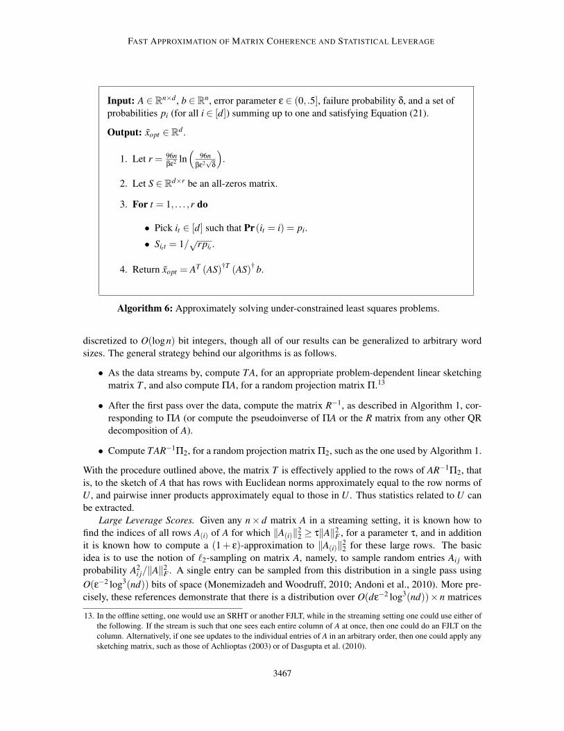
FAST APPROXIMATION OF MATRIX COHERENCE AND STATISTICAL LEVERAGE
Input: A ∈ Rn×d , b ∈ R
n, error parameter ε ∈ (0, .5], failure probability δ, and a set of
probabilities pi (for all i ∈ [d]) summing up to one and satisfying Equation (21).
Output: xopt ∈ Rd .
1. Let r = 96nβε2 ln
(
96n
βε2√
δ
)
.
2. Let S ∈ Rd×r be an all-zeros matrix.
3. For t = 1, . . . ,r do
• Pick it ∈ [d] such that Pr(it = i) = pi.
• Sit t = 1/√
rpit .
4. Return xopt = AT (AS)†T (AS)†b.
Algorithm 6: Approximately solving under-constrained least squares problems.
discretized to O(logn) bit integers, though all of our results can be generalized to arbitrary word
sizes. The general strategy behind our algorithms is as follows.
• As the data streams by, compute TA, for an appropriate problem-dependent linear sketching
matrix T , and also compute ΠA, for a random projection matrix Π.13
• After the first pass over the data, compute the matrix R−1, as described in Algorithm 1, cor-
responding to ΠA (or compute the pseudoinverse of ΠA or the R matrix from any other QR
decomposition of A).
• Compute TAR−1Π2, for a random projection matrix Π2, such as the one used by Algorithm 1.
With the procedure outlined above, the matrix T is effectively applied to the rows of AR−1Π2, that
is, to the sketch of A that has rows with Euclidean norms approximately equal to the row norms of
U , and pairwise inner products approximately equal to those in U . Thus statistics related to U can
be extracted.
Large Leverage Scores. Given any n× d matrix A in a streaming setting, it is known how to
find the indices of all rows A(i) of A for which ‖A(i)‖22 ≥ τ‖A‖2
F , for a parameter τ, and in addition
it is known how to compute a (1+ ε)-approximation to ‖A(i)‖22 for these large rows. The basic
idea is to use the notion of ℓ2-sampling on matrix A, namely, to sample random entries Ai j with
probability A2i j/‖A‖2
F . A single entry can be sampled from this distribution in a single pass using
O(ε−2 log3(nd)) bits of space (Monemizadeh and Woodruff, 2010; Andoni et al., 2010). More pre-
cisely, these references demonstrate that there is a distribution over O(dε−2 log3(nd))×n matrices
13. In the offline setting, one would use an SRHT or another FJLT, while in the streaming setting one could use either of
the following. If the stream is such that one sees each entire column of A at once, then one could do an FJLT on the
column. Alternatively, if one see updates to the individual entries of A in an arbitrary order, then one could apply any
sketching matrix, such as those of Achlioptas (2003) or of Dasgupta et al. (2010).
3467

DRINEAS, MAGDON-ISMAIL, MAHONEY AND WOODRUFF
T for which for any fixed matrix A ∈ Rn×d , there is a procedure which given TA, outputs a sample
(i, j) ∈ [n]× [d] with probability (1± ε)A2
i, j
‖A‖2F
± n−O(1). Technically, these references concern sam-
pling from vectors rather than matrices, so T (A) is a linear operator which treats A as a length-nd
vector and applies the algorithm of Monemizadeh and Woodruff (2010) and Andoni et al. (2010).
However, by simply increasing the number of rows in T by a factor of the small dimension d, we
can assume T is left matrix multiplication. By considering the marginal along [n], the probability
that i = a, for any a ∈ [n], is
(1± ε)‖U(a)‖2
2
‖U‖2F
± (nd)−O(1).
By the coupon collector problem, running O(τ−1 logτ−1) independent copies is enough to find a set
containing all rows A(i) for which ‖A(i)‖22 ≥ τ‖A‖2
F , and no rows A(i) for which ‖A(i)‖22 < τ
2‖A‖2
F
with probability at least 0.99.
When applied to our setting, we can apply a random projection matrix Π and a linear sketching
matrix T which has O(dτ−1ε−2 log3(n) logτ−1) rows in the following manner. First, TA and ΠA
are computed in the first pass over the data; then, at the end of the first pass, we compute R−1;
and finally, we compute TAR−1Π2, for a random projection matrix Π2. This procedure effectively
applies the matrix T to the rows of AR−1Π2, which have norms equal to the row norms of U , up to a
factor of 1+ ε. The multiplication at the end by Π2 serves only to speed up the time for processing
TAR−1. Thus, by the results of Monemizadeh and Woodruff (2010) and Andoni et al. (2010), we
can find all the leverage scores ‖U(i)‖22 that are of magnitude at least τ‖U‖2
F in small space and a
single pass over the data. By increasing the space by a factor of O(ε−2 logn), we can also use the
ℓ2-samples to estimate the norms ‖U(i)‖22 for the row indices i that we find.
Entropy. Given a distribution ρ, a statistic of ρ of interest is the entropy of this distribution,
where the entropy is defined as H(ρ) = ∑i ρ(i) log2(1/ρ(i)). This statistic can be approximated in
a streaming setting. Indeed, it is known that estimating H(ρ) up to an additive ε can be reduced
to (1 + ε)-approximation of the ℓp-norm of the vector (ρ(1), . . . ,ρ(n)), for O(log1/ε) different
p ∈ (0,1) (Harvey et al., 2008). Here ε = ε/(log3 1/ε · logn). When applied to our setting, the
distribution of interest is ρ(i) = 1d‖U(i)‖2
2. To compute the entropy of this distribution, there exist
sketching matrices T for providing (1+ε)-approximations to the quantity Fp(F2) of an n×d matrix
A, where Fp(F2) is defined as ∑ni=1 ‖A(i)‖2p
2 , using O(ε−4 log2 n log1/ε) bits of space (see Theorem
1 of Ganguly et al. (2008)). Thus, to compute the entropy of the leverage score distribution, we
can do the following. First, maintain TA and ΠA in the first pass over the data, where T is a
sketching matrix for Fp(F2), p ∈ (0,1). At the end of the first pass, compute R−1; and finally,
compute TAR−1Π2, which effectively applies the Fp(F2)-estimation matrix T to the rows of the
matrix AR−1Π2. Therefore, by the results of Harvey et al. (2008) and Ganguly et al. (2008), we can
compute an estimate φ which is within an additive ε of H(ρ) using O(dε−4 log6 n log14 1/ε) bits of
space and a single pass. We note that it is also possible to estimate H(ρ) up to a multiplicative 1+ε
factor using small, but more, space; see, for example, Harvey et al. (2008).
Sampling Row Identities. Another natural problem is that of obtaining samples of rows of
A proportional to their leverage score importance sampling probabilities. To do so, we use ℓ2-
sampling (Monemizadeh and Woodruff, 2010; Andoni et al., 2010) as used above for finding the
large leverage scores. First, compute TA and ΠA in the first pass over the data stream; then, compute
R−1; and finally, compute TAR−1. Thus, by applying the procedures of Andoni et al. (2010) a total
of s times independently, we obtain s samples i1, . . . , is, with replacement, of rows of A proportional
3468
FAST APPROXIMATION OF MATRIX COHERENCE AND STATISTICAL LEVERAGE
to ‖U(i1)‖22, . . . ,‖U(is)‖2
2, that is, to their leverage score. The algorithm requires O(sdε−2 log4 n) bits
of space and runs in a single pass. To obtain more than just the row identities i1, . . . , is, for example,
to obtain the actual samples, one can read off these rows from A in a second pass over the matrix.
References
D. Achlioptas. Database-friendly random projections: Johnson-lindenstrauss with binary coins.
Journal of Computer and System Sciences, 66(4):671–687, 2003.
N. Ailon and B. Chazelle. Approximate nearest neighbors and the fast Johnson-Lindenstrauss trans-
form. In Proceedings of the 38th Annual ACM Symposium on Theory of Computing, pages 557–
563, 2006.
N. Ailon and B. Chazelle. The fast Johnson-Lindenstrauss transform and approximate nearest neigh-
bors. SIAM Journal on Computing, 39(1):302–322, 2009.
N. Ailon and E. Liberty. Fast dimension reduction using Rademacher series on dual BCH codes.
In Proceedings of the 19th Annual ACM-SIAM Symposium on Discrete Algorithms, pages 1–9,
2008.
A. Andoni, R. Krauthgamer, and K. Onak. Streaming algorithms from precision sampling. Techni-
cal report, 2010. Preprint: arXiv:1011.1263.
H. Avron, P. Maymounkov, and S. Toledo. Blendenpik: Supercharging LAPACK’s least-squares
solver. SIAM Journal on Scientific Computing, 32:1217–1236, 2010.
C. Bekas, E. Kokiopoulou, and Y. Saad. An estimator for the diagonal of a matrix. Applied Numer-
ical Mathematics, 57:1214–1229, 2007.
C. Bekas, A. Curioni, and I. Fedulova. Low cost high performance uncertainty quantification. In
Proceedings of the 2nd Workshop on High Performance Computational Finance, page Article
No.: 8, 2009.
P. Bonacich. Power and centrality: A family of measures. The American Journal of Sociology, 92
(5):1170–1182, 1987.
C. Boutsidis, M.W. Mahoney, and P. Drineas. An improved approximation algorithm for the column
subset selection problem. In Proceedings of the 20th Annual ACM-SIAM Symposium on Discrete
Algorithms, pages 968–977, 2009.
C. Boutsidis, P. Drineas, and M. Magdon-Ismail. Near-optimal column-based matrix reconstruction.
In Proceedings of the 52nd Annual IEEE Symposium on Foundations of Computer Science, pages
305–314, 2011a.
C. Boutsidis, P. Drineas, and M. Magdon-Ismail. Near-optimal column-based matrix reconstruction.
Technical report, 2011b. Preprint: arXiv:1103.0995.
E.J. Candes and B. Recht. Exact matrix completion via convex optimization. Technical report,
2008. Preprint: arXiv:0805.4471.
3469
DRINEAS, MAGDON-ISMAIL, MAHONEY AND WOODRUFF
S. Chatterjee and A.S. Hadi. Influential observations, high leverage points, and outliers in linear
regression. Statistical Science, 1(3):379–393, 1986.
S. Chatterjee and A.S. Hadi. Sensitivity Analysis in Linear Regression. John Wiley & Sons, New
York, 1988.
S. Chatterjee, A.S. Hadi, and B. Price. Regression Analysis by Example. John Wiley & Sons, New
York, 2000.
A. Dasgupta, R. Kumar, and T. Sarlos. A sparse Johnson-Lindenstrauss transform. In Proceedings
of the 42nd Annual ACM Symposium on Theory of Computing, pages 341–350, 2010.
P. Drineas, R. Kannan, and M.W. Mahoney. Fast Monte Carlo algorithms for matrices I: Approxi-
mating matrix multiplication. SIAM Journal on Computing, 36:132–157, 2006a.
P. Drineas, M.W. Mahoney, and S. Muthukrishnan. Sampling algorithms for ℓ2 regression and
applications. In Proceedings of the 17th Annual ACM-SIAM Symposium on Discrete Algorithms,
pages 1127–1136, 2006b.
P. Drineas, M.W. Mahoney, and S. Muthukrishnan. Relative-error CUR matrix decompositions.
SIAM Journal on Matrix Analysis and Applications, 30:844–881, 2008.
P. Drineas, J. Lewis, and P. Paschou. Inferring geographic coordinates of origin for Europeans using
small panels of ancestry informative markers. PLoS ONE, 5(8):e11892, 2010a.
P. Drineas, M.W. Mahoney, S. Muthukrishnan, and T. Sarlos. Faster least squares approximation.
Numerische Mathematik, 117(2):219–249, 2010b.
S. Ganguly, M. Bansal, and S. Dube. Estimating hybrid frequency moments of data streams. In
Proceedings of the 2nd Annual International Workshop on Frontiers in Algorithmics, pages 55–
66, 2008.
S. Georgiev and S. Mukherjee, 2011. Unpublished results. (2011).
A. Gittens and M. W. Mahoney, 2012. In preparation. (2012).
G.H. Golub and C.F. Van Loan. Matrix Computations. Johns Hopkins University Press, Baltimore,
1996.
N. Halko, P.-G. Martinsson, and J. A. Tropp. Finding structure with randomness: Probabilistic
algorithms for constructing approximate matrix decompositions. SIAM Review, 53(2):217–288,
2011.
N.J.A. Harvey, J. Nelson, and K. Onak. Sketching and streaming entropy via approximation theory.
In Proceedings of the 49th Annual IEEE Symposium on Foundations of Computer Science, pages
489–498, 2008.
D.C. Hoaglin and R.E. Welsch. The hat matrix in regression and ANOVA. The American Statisti-
cian, 32(1):17–22, 1978.
3470
FAST APPROXIMATION OF MATRIX COHERENCE AND STATISTICAL LEVERAGE
E. A. Jonckheere, M. Lou, J. Hespanha, and P. Barooah. Effective resistance of Gromov-hyperbolic
graphs: Application to asymptotic sensor network problems. In Proceedings of the 46th IEEE
Conference on Decision and Control, pages 1453–1458, 2007.
M. Magdon-Ismail. Row sampling for matrix algorithms via a non-commutative Bernstein bound.
Technical report, 2010. Preprint: arXiv:1008.0587.
M. W. Mahoney. Randomized Algorithms for Matrices and Data. Foundations and trends in machine
learning. NOW Publishers, Boston, 2011. Also available at: arXiv:1104.5557.
M.W. Mahoney and P. Drineas. CUR matrix decompositions for improved data analysis. Proc. Natl.
Acad. Sci. USA, 106:697–702, 2009.
X. Meng, M. A. Saunders, and M. W. Mahoney. LSRN: A parallel iterative solver for strongly over-
or under-determined systems. Technical report, 2011. Preprint: arXiv:1109.5981.
M. Monemizadeh and D. P. Woodruff. 1-pass relative-error lp-sampling with applications. In Pro-
ceedings of the 21st Annual ACM-SIAM Symposium on Discrete Algorithms, pages 1143–1160,
2010.
S. Muthukrishnan. Data Streams: Algorithms and Applications. Foundations and Trends in Theo-
retical Computer Science. Now Publishers Inc, Boston, 2005.
M.Z. Nashed, editor. Generalized Inverses and Applications. Academic Press, New York, 1976.
M.E.J. Newman. A measure of betweenness centrality based on random walks. Social Networks,
27:39–54, 2005.
C.H. Papadimitriou, P. Raghavan, H. Tamaki, and S. Vempala. Latent semantic indexing: a proba-
bilistic analysis. Journal of Computer and System Sciences, 61(2):217–235, 2000.
P. Paschou, E. Ziv, E.G. Burchard, S. Choudhry, W. Rodriguez-Cintron, M.W. Mahoney, and
P. Drineas. PCA-correlated SNPs for structure identification in worldwide human populations.
PLoS Genetics, 3:1672–1686, 2007.
P. Paschou, J. Lewis, A. Javed, and P. Drineas. Ancestry informative markers for fine-
scale individual assignment to worldwide populations. Journal of Medical Genetics, page
doi:10.1136/jmg.2010.078212, 2010.
M. Richardson and P. Domingos. Mining knowledge-sharing sites for viral marketing. In Proceed-
ings of the 8th Annual ACM SIGKDD Conference, pages 61–70, 2002.
V. Rokhlin and M. Tygert. A fast randomized algorithm for overdetermined linear least-squares
regression. Proc. Natl. Acad. Sci. USA, 105(36):13212–13217, 2008.
V. Rokhlin, A. Szlam, and M. Tygert. A randomized algorithm for principal component analysis.
SIAM Journal on Matrix Analysis and Applications, 31(3):1100–1124, 2009.
T. Sarlos. Improved approximation algorithms for large matrices via random projections. In Pro-
ceedings of the 47th Annual IEEE Symposium on Foundations of Computer Science, pages 143–
152, 2006.
3471

DRINEAS, MAGDON-ISMAIL, MAHONEY AND WOODRUFF
A. Talwalkar and A. Rostamizadeh. Matrix coherence and the Nystrom method. In Proceedings of
the 26th Conference in Uncertainty in Artificial Intelligence, 2010.
P.F. Velleman and R.E. Welsch. Efficient computing of regression diagnostics. The American
Statistician, 35(4):234–242, 1981.
3472