Fast Computation of Supertrees for Compatible

Phylogenies with Nested Taxa

Vincent Berry1 and Charles Semple2,3

8 November 2005

1Departement Informatique, L.I.R.M.M. - C.N.R.S., 161 rue Ada, 34392 MontpellierCedex 5, Francevberry@lirmm.fr

2Biomathematics Research Centre, Department of Mathematics and Statistics, Universityof Canterbury, Christchurch, New Zealandc.semple@math.canterbury.ac.nz

3Corresponding author.

Keywords. Phylogenetics, supertree methods, nested taxa, compatibility, strepsirrhinephylogeny.

Abstract

Typically, supertree methods combine a collection of source trees in which justthe leaves are labelled by taxa. In such methods the resulting supertree is also leaf-labelled. An underlying assumption in these methods is that, across all trees in thecollection, no two of the taxa are nested; for example, “buttercups” and “plants”are nested taxa. Motivated by Page, the first supertree algorithm for allowing thesource trees to collectively have nested taxa is called AncestralBuild. Here, inaddition to taxa labelling the leaves, the source trees may have taxa labelling someof their interior nodes. Taxa labelling interior nodes are at a higher taxonomic levelthan that of their descendants (for example, genera versus species). Analogous tothe supertree method Build for deciding the compatibility of a collection of sourcetrees in which just the leaves are labelled, AncestralBuild is a polynomial-timealgorithm for deciding the compatibility of a collection of source trees in which someof the interior nodes are also labelled by taxa. Although a more general method,in this paper we show that the original description of AncestralBuild can bemodified so that the running time is as fast as the current fastest running time for

1

Build. Fast computation for deciding compatibility is essential if one is to makeuse of phylogenetic databases that contain thousands of trees on tens of thousandsof taxa. This is particularly so as AncestralBuild is incorporated as a basic toolinside more general supertree methods (that is, methods that always output a treeregardless of the compatibility of the source trees). We apply the method to proposea comprehensive phylogeny of the strepsirrhines, a major group of the primates.

2

Introduction

Supertree methods are a fundamental and practical way of inferring phylogenies. Generallyspeaking, these methods amalgamate a collection of “source” trees on overlapping subsetsof taxa into a single parent tree that contains the taxa of all of the source trees. This parenttree is called a supertree. This approach to constructing evolutionary trees is particularlyappealing because it allows the inference of an evolutionary scenario from a combinationof analyses differing in the set of taxa they encompass as well as in the primary datafrom which they were conducted (for example, molecular or morphological studies). Theincreasing popularity of these methods and the diversity of ways in which they can be usedis highlighted in a recently published book (Bininda-Emonds, 2004).

Historically, supertree methods only make use of the leaf labels of the source trees,with the resulting supertree having the property that taxa are only attached at leaves. Onthis basis, supertree methods can deal with taxa at different taxonomic levels only in thecase where the leaves of the source trees represent non-nested taxa (e.g., “elephant” and“mammal” should not be represented as two distinct leaves amongst the source trees as theformer taxa is nested inside the latter taxa). However, in supertree studies this situationdoes occur, especially concerning outgroups. For example, a source tree containing strep-sirrhine species could include Haplorrhini, a sub-order, as an outgroup leaf, and anothersource tree on primates would include several haplorrhine species as leaves, while the lat-ter are nested inside the former taxon. Because of the assumption that taxa of the sourcetrees are non-nested, traditional supertree methods produce in that case an incorrect su-pertree. Thus, unless one resorts to preprocessing of source trees to remove nested taxa viataxonomic synonymy (Bininda-Emonds et al., 2004), traditional supertree methods havelimited use in the case of nested taxa, as arises when one is to amalgamate trees fromphylogenetic databases such as TreeBASE (Sanderson et al., 1993). This was recentlyhighlighted by Page (2004). Indeed, TreeBASE incorporates trees from many differentpublished phylogenetic studies that focus on a variety of different biological problems, andhence consider evolutionary relationships at different taxonomic levels.

As a consequence of this limitation, Page (2004) motivated the task of designing su-pertree methods that allow the interior nodes as well as all of the leaves to represent taxain the source trees. In these nested-taxa source trees, an interior label corresponds to ataxon at a higher taxonomic level than any of its descendants. Note that interior labelscan be either available initially in the source trees, or added to some source trees basedon taxa present in other source trees at the time the collection of studied source trees isformed. The first computational problem that arises is to find a polynomial-time algorithmfor deciding whether or not a collection of nested-taxa source trees is compatible and, ifso, constructing an appropriate supertree.

In answer to this problem, Daniel and Semple (2004) provided an algorithm calledAncestralBuild. This algorithm generalizes Build, one of the first supertree methods(Aho et al., 1981). The polynomial-time algorithm Build takes a collection P of rooted

3

leaf-labelled trees as input and decides whether or not P is compatible, in which case itreturns a leaf-labelled supertree that displays P. That is, the supertree preserves all ofthe relative groupings of taxa present in the source trees. For a collection of nested-taxatrees, if a supertree preserves all ancestral relationships as well as all groupings of taxa,then the supertree is said to ancestrally display this collection and the collection is saidto be ancestrally compatible. These concepts are formally defined in the next section.However, we make a comment here on the way in which ancestor is used in this paper: bywriting that a taxon t is an ancestor of a taxon t′, we mean that t is either a hypotheticalancestral taxon of t′ or that t is the name of a taxonomic grouping containing t′, so thatnode labelled t is ancestral to the node labelled t′. The algorithm AncestralBuildtakes a collection P of nested-taxa trees as input and outputs a supertree that ancestrallydisplays P if such a supertree exists, otherwise it states that the collection is not ancestrallycompatible. Though designed to handle trees containing taxa at both internal nodes andleaves, AncestralBuild also accepts collections of source trees that have taxa only at theleaves, because leaf-labelled trees are a special case of nested-taxa trees. In that particularcase, AncestralBuild decides the compatibility of the source trees in the usual sense.Consequently, it does indeed generalize Build.

AncestralBuild has the desirable property to give an exact answer in polynomial-time (Daniel and Semple, 2004). However, there can be three objections to its use. First,for incompatible phylogenies to be combined, an all-or-nothing algorithm, that is just stat-ing the incompatibility when it arises, is not desirable. Second, even for the easiest case ofsource trees that are all fully-resolved and have taxa only at the leaves, the running timeof the version of AncestralBuild stated in Daniel and Semple (2004) is O(t2n3), wheret is the number of source trees and n is the number of taxa. Despite being polynomial,this running time makes AncestralBuild a reasonably slow algorithm in practice, par-ticularly if it is to handle the thousands of trees stored in databases such as TreeBASE.Third, in the absence of internal labels in the source trees, the method will build a nonsen-sical supertree, not knowing for instance that the “mammal” taxon met in one tree is anancestor of “elephant”, present in another tree. We answer these three objections below.

Inferring a supertree for incompatible source trees. Primary data sequences aregetting longer and phylogenetic methods more accurate, so that a reasonable number ofpublished phylogenies are compatible. For example, Llabres et al. (2005) found a very lowrate of incompatible trees in TreeBASE. However, it is still relatively frequent that one hasto deal with incompatible source trees. For example, it is well-known that gene trees mayconflict with species trees (due to e.g., lateral gene transfer or hybridization), and that sometrees may contain erroneous branches inferred due to noisy information for some internaledges in the primary data. In the former case, one may want to construct a supertree toidentify the disagreements between the gene trees and the species trees. In such cases, anall-or-nothing algorithm may not be enough and one can understandably prefer a moregeneral supertree method that outputs a supertree that either conflicts with or omits someinformation present in the source trees. However, for any general supertree method, a

4

basic property that one would always like is that of consistency; that is, if the source treescarry no conflicting information, then the supertree returned by the method displays eachof the source trees. Because the property of consistency is such a compelling property,many general supertree methods dealing with leaf-labelled trees (respectively, nested-taxatrees) are likely either to have Build (respectively, AncestralBuild) as a subroutineor to be a variant of Build (respectively, AncestralBuild). Indeed, this is alreadythe case for some general methods: both MinCutSupertree (Semple and Steel, 2000)method and its modified version (Page, 2002) are variants of Build and, more recently,Daniel and Semple (2005) describe a class of general supertree methods for nested-taxasource trees that is a variant of AncestralBuild. (This class and more particularlythe underlying general supertree method NestedSupertree is described further in thelast section.) Moreover, these all-or-nothing algorithms can be repeatedly used in simpleschemes to extract compatible parts out of a collection of incompatible source trees. Wehighlight two examples of such schemes in the discussion part of this paper.

Reasonable running time. Given the amount of information in current tree databases,it is not unreasonable to try to amalgamate hundreds of trees that collectively contain thou-sands of taxa and, consequently, fast algorithms are essential. To deal with fully-resolved(i.e., binary) leaf-labelled trees, Henzinger et al. (1999) proposed a fast implementation

of Build that runs in O(mn1

2 ) time, where m is the total sum of the number of nodes ineach of the source trees and n is the total number of taxa. (They also proposed a variantof Build running in O(m + n2 log n) time but, in the case of compatibility, it typicallyresulted in a supertree with edges not supported by any part of the data, an undesirablefeature for a supertree algorithm.) For comparison between this running time and theO(t2n3) running time of AncestralBuild, note that m can range from O(n) to O(tn).Thus, the running time of AncestralBuild as stated in Daniel and Semple (2004) isstill relatively slow compared to the implementation provided by Henzinger et al. (1999)for Build in the special case of fully-resolved leaf-labelled trees. However, comparing thegap between these running times provides hope for improving AncestralBuild on thisaspect, despite the latter being a much more general algorithm for it allows nested-taxatrees and trees that are partially resolved. In this paper we describe several modificationsto AncestralBuild that greatly reduce its computational complexity. Some of thesemodifications have a similar flavour to techniques used in Henzinger et al. (1999). Therunning time of AncestralBuild resulting from these modifications is as fast as thecurrent fastest algorithm for source trees in which only the leaves are labelled (Henzingeret al., 1999). More particularly, the achieved running time is almost linear in the size ofthe source trees, when these trees are fully-resolved. Furthermore, extending the imple-mentation of Henzinger et al. (1999) for Build in the most canonical and efficient way toallow partially-resolved leaf-labelled trees in its input, we also show that the running timeof our modification of AncestralBuild is the same as that for this extension of Build.

5

Having a sensible supertree as output. In the case where nested taxa are present indifferent source trees but these trees contain no internal label, then, unless extra informa-tion is provided to recognize such nestings, there is no chance that AncestralBuild (orany supertree method) produces a sensible supertree. For example, if one tree contains “ele-phant” and another “mammal” without any tree indicating that the latter is an ancestorof the former, then the supertree output by the methods will have both taxa as tips. Thissituation arises because of lack of information in the source trees. Unfortunatly, this willbe a frequent situation in practice because already inferred trees are usually stored withoutinternal labels, though this is allowed by the Newick format. In such a case, all that isrequired for the method to produce a sensible supertree is a (partial) reference taxonomy in-dicating the nestings between taxa of interest. This taxonomy can be included as one extrasource tree or be divided into several extra very simple trees of two vertices, where an ances-tor taxon is above one of its descendant taxon. This reference taxonomy can be either builtby hand, or generated automatically by a program searching taxon names in web accessibletaxonomies, like NCBI’s Taxonomy Browser (http://www.ncbi.nlm.nih.gov/entrez) orthe Tree of Life web site (http://tolweb.org/tree). See Page and Valiente (2005) andHibbett et al. (2005) for programs filling aims close to that one.

To describe an application of AncestralBuild, we studied the evolutionary rela-tionships of the Strepsirrhini, one of the two major primate groups. Monophyly of thisgroup is widely accepted but some intrasubordinal relationships were still recently underdebate. Recent studies investigating strepsirrhine phylogeny involve quite different kindsof data, including mtDNA sequences (Yoder et al., 2000), craniodental morphological data(Masters and Brothers, 2002) and retroposon analysis (Roos et al., 2004). We appliedAncestralBuild to four phylogenies published in these papers, covering many differenttaxonomic levels from order to individuals. The method shows that these phylogenies areancestrally compatible and provides as result a comprehensive supertree of the Strepsir-rhini. This highlights, once again, the interest in the supertree approach, that allows tocombine phylogenies inferred from different kinds of primary data.

The rest of the paper is organized as follows. The next section contains some pre-liminaries that are used throughout the paper. The following three sections contain adescription of AncestralBuild as stated in Daniel and Semple (2004) and descriptionsof our modifications of this algorithm as well as the running time of this modification.An application of AncestralBuild to obtain a strepsirrhine supertree is described inthe following section. In addition to deciding compatibility, AncestralBuild can beused in a variety of ways for constructing supertrees from incompatible source trees. Wehighlight some of these ways in the last section. Finally, the appendix contains the proofwhich establishes that our modification of AncestralBuild does indeed decide ancestralcompatibility for a collection of nested-taxa trees as well as a pseudo-code description ofthis algorithm.

We end the introduction by noting that a novel approach for testing the ancestralcompatibility of two rooted semi-labelled trees has been recently proposed by Llabres

6

y e c d fa bdc f e

T1 T2

x

z x

z

T3

y

Figure 1: A compatible collection P of rooted semi-labelled trees.

et al. (2005).

Preliminaries

In this section, we describe some concepts that are frequently used in the paper. Forfurther details, we refer the interested reader to Semple and Steel (2003).

Phylogenies. The degree of a node v in a graph (or, in particular, a tree) is the number ofedges incident with v. We denote the degree of v by d(v). Essentially, a rooted phylogeneticX-tree is a rooted tree whose leaves are labelled with the elements of a set X of taxa. Weformally define it as follows. A rooted phylogenetic tree (on X) is an ordered pair (T ; φ)consisting of a rooted tree T in which all interior nodes have degree at least three exceptthe root which has degree at least two, and a map φ from X to the leaf set of T thatassigns each element in X to a leaf in T so that no two elements are assigned the sameleaf in T and each leaf of T is assigned an element of X. A rooted phylogenetic tree isfully-resolved or binary if the root of T has degree two and all other interior nodes of Thave degree three.

The concept of rooted phylogenetic trees naturally extends to trees in which some ofthe interior nodes are also labelled by taxa. Such trees, called nested-taxa trees or rootedsemi-labelled trees, are used to display in the same tree taxa at different taxonomic levels.More precisely, a rooted semi-labelled tree T on a taxa set X is an ordered pair (T ; φ)consisting of a rooted tree T with root node ρ, and a map φ from X into the node set Vof T such that, for all non-root nodes v of degree at most two, φ assigns v an element ofX, and if ρ has degree zero or one, then φ also assigns ρ an element of X. If every nodeof T is assigned at most one taxa of X under φ, then T is said to be singularly labelled.Furthermore, if T is singularly labelled and the degree of any node in T is at most threeexcept for the root which has degree at most two, then we say that T is binary. In Figure 1,each of T1, T2, and T3 is a rooted semi-labelled tree, but T3 is the only rooted semi-labelledtree that is binary.

Remarks.

7

1. We will often write a rooted semi-labelled X-tree for a rooted semi-labelled tree on X.

2. Observe that rooted phylogenetic trees are special types of rooted semi-labelled trees.

3. To simplify matters and because we see no practical reason for nodes in the source treesto be assigned more than one taxa of X, we will assume throughout the paper thatall rooted semi-labelled trees that are source trees are singularly labelled. However, wenote that the upgrade of the results in this paper to non-singular rooted semi-labelledtrees is straightforward. Note that this remark about singular labelling does not applyto the output tree, where it is quite possible that some nodes are labelled with morethan one taxa. For instance, a node joining human and chimp on a source tree thatcontains no other mammals could be equally labelled as anything from “hominoid” to“primate” to “mammal”. This multiple listing of a node then becomes very importantif all these names appear on other source trees and there is no user-input taxonomy tosort this out.

Let T = (T ; φ) be a rooted semi-labelled tree on X. The set X is called the label setof T and we call the elements of X labels. We also use L(T ) to denote the label set of T .For example, in Figure 1, L(T1) = {c, d, e, f, x, y}. For a node v of T , we denote the set ofelements of X that are assigned to v by φ−1(v) and say that the elements in φ−1(v) labelv. Furthermore, T is fully labelled if every node of T is labelled by an element of X. Fora collection P of rooted semi-labelled trees, we denote the union of the label sets of thetrees in P by L(P). Thus, for example, for the collection P of rooted semi-labelled treesshown in Figure 1, we have L(P) = {a, b, c, d, e, f, x, y, z}.

Let T = (T ; φ) be a rooted semi-labelled tree, and let a, b ∈ L(T ). We say that a is adescendant (label) of b (or, alternatively, b is an ancestor (label) of a) if the path from theroot of T to φ(a) includes φ(b). Furthermore, a and b are not comparable if neither a is adescendant of b nor b is a descendant of a. Now suppose that a and b are not comparablein T . Then the node of T that is the last common node on the paths from the root of Tto φ(a) and from the root of T to φ(b) is called the most recent common ancestor of a andb, and is denoted mrcaT (a, b).

Lastly, throughout the paper, for a rooted semi-labelled tree T , we will use |T | todenote the number of nodes in T . Furthermore, for a collection P of rooted semi-labelledtrees, we will use m to denote

∑

T ∈P|T |.

Compatibility. We will describe the notion of compatibility for rooted phylogenetic treesfirst, before extending this notion to rooted semi-labelled trees.

Let T be a rooted phylogenetic tree on X and let T ′ be a rooted phylogenetic tree onX ′, where X is a subset of X ′. We say that T ′ displays T if, up to suppressing all non-rootnodes of degree-two, the minimal rooted subtree of T ′ that connects the elements in X isa refinement of T , that is T can be obtained from it by contracting edges. Suppressing adegree-two node v means replacing v and its two incident edges with a single edge. Observe

8

c d

y

f e a b

x

z

Figure 2: A rooted semi-labelled tree that ancestrally displays the collection P of treesshown in Figure 1. Indeed, as we shall soon see, this is the tree outputted by Ancestral-Build when applied to P.

that the use of “refinement” means that we allow for the resolution of soft polytomies inthe definition of displays, where we recall that a soft polytomy represents an uncertaintyas to the exact order of speciation as oppose to a certainty of a multiple speciation event.A collection P of rooted phylogenetic trees are compatible if there is a rooted phylogenetictree T that simultaneously displays each of the trees in P, in which case we say that Tdisplays P.

The notion of displays for rooted semi-labelled trees extends the notion of displays forrooted phylogenetic trees. In particular, let T be a rooted semi-labelled X-tree and let T ′

be a rooted semi-labelled X ′-tree, where X is a subset of X ′. Then T ′ ancestrally displaysT if, up to suppressing non-root nodes of degree-two, the minimal rooted subtree of T ′

that connects the elements in X is a refinement of T and, for all a, b ∈ X, whenever ais a descendant label of b in T , we have that a is a descendant label of b in this rootedsubtree. A collection P of rooted semi-labelled trees is ancestrally compatible if there isa rooted semi-labelled tree T that ancestrally displays each of the trees in P, in whichcase we say that T ancestrally displays P. To illustrate this notion, the collection of treesin Figure 1 is ancestrally compatible, as each of its trees is ancestrally displayed by therooted semi-labelled tree shown in Figure 2.

It is important to note that a collection of rooted semi-labelled trees may be ancestrallyincompatible because of their interior labels and not their leaf labels. This could be assimple as a contradiction on an ancestor-descendant relationship, or as complex as theincompatibility of a set of most recent common ancestor relationships.

Graphs and Digraphs. Let G be a graph with node set V . We frequently use thenotation {u, v} to denote the edge joining the nodes u and v. Furthermore, the connectedcomponents of G are the subgraphs of G such that, for all u, v ∈ V , u and v are in thesame connected component if and only if there is a path from u to v.

A directed graph, also called a digraph, is simply a graph in which, instead of havingedges joining two nodes, we have directed edges; that is, edges directed from one node toanother. Directed edges are also called arcs. We use the notation (u, v) to denote the arcdirected from u to v. For a directed graph D, the indegree of a node v is the number of arcs

9

directed into v and the outdegree of v is the number of arcs directed out of v. Analogous tothe connected components of an ordinary graph, the (connected) arc components of D arethe sub-digraphs of D such that, for all u, v ∈ V , u and v are in the same arc componentif and only if, ignoring the direction of the arcs, there is a path between u and v.

For the purposes of this paper, we say that a graph is mixed if it contains both arcs andedges. An arc component of a mixed graph is an arc component of the digraph obtainedwhen masking the edges of this graph.

Let D be a (mixed) graph, let v be a node of D, and let U be a subset of the set ofnodes of D. The (mixed) graph obtained from D by deleting v and each of its incidentarcs and edges is denoted by D\v. In general, we use D\U to denote the graph obtainedfrom D by deleting each of the nodes in U . Furthermore, if V is the node set of D, thenthe restriction of D to U (also called the subgraph of D induced by U) is the subgraph ofD that is obtained by deleting each of the nodes in V − U . This subgraph is denoted byD|U .

Finally, one typically views a rooted tree as an undirected graph. However, it will oftenbe convenient in this paper to view a rooted tree as a directed graph where each edge isreplaced with an arc directed away from the root.

AncestralBuild

For completeness and to make a comparison of the modifications we describe in this paper,in this section we give a full description of AncestralBuild as it is stated in Daniel andSemple (2004).

We begin by describing a construction on a collection of rooted semi-labelled trees, and aparticular mixed graph on a collection of rooted fully-labelled trees. Both the constructionand mixed graph are central to AncestralBuild.

Let T = (T ; φ) be a rooted semi-labelled tree on X, where T has node set V . We saythat a rooted fully-labelled tree T ′ has been obtained from T by adding distinct new labelsif, for each node of T that is not assigned a label under φ, we assign it an arbitrary labelnot in X so that no two new labels are the same. In general, if P is a collection of rootedsemi-labelled trees, we say that P ′ has been obtained from P by adding distinct new labelsif it has been obtained by adding distinct new labels to each tree in P so that across alltrees in P ′ no two new labels are the same.

Example 1 To illustrate the above construction, let P be the collection of rooted semi-labelled trees shown in Figure 1. The collection P ′ shown in Figure 3 has been obtainedfrom P by adding distinct new labels. Note that the added labels only need to be unique,

10

y e c d fa bc f e

T ′1 T ′

2

x

z mrcaT3(c, d)

yx

d

mrcaT1(x, y)

mrcaT1(e, y)

z

T ′3

mrcaT2(e, z)

Figure 3: A collection P ′ of rooted fully-labelled trees.

mrcaT2(e, z) mrcaT3

(c, d)

mrcaT1(x, y)

d

x

y

e

a b z

f

mrcaT1(e, y)

c

Figure 4: The descendancy graph of P ′. Arcs are shown as dashed lines with an arrowshowing the direction of the arc, while edges are shown as solid lines.

and not as involved as the ones shown in Figure 3. The reason for choosing these particularlabels will be made clear in the next section. 2

Let P ′ be a collection of rooted fully-labelled trees. The descendancy graph of P ′,denoted D(P ′), is the mixed graph whose node set is L(P ′), and whose arc and edge setsare

{

(c, a) : a is a descendant label of c in some T in P ′}

and{

{a, b} : a is not comparable to b in some T in P ′}

,

respectively. Figure 4 shows the descendancy graph corresponding to the collection P ′ ofrooted fully-labelled trees shown in Figure 3.

We now describe AncestralBuild. All of the work in the algorithm is performed bya subroutine called Descendant which decides the ancestral compatibility of a collectionP ′ of rooted fully-labelled trees that has been obtained from the original collection P ofrooted semi-labelled trees by adding distinct new labels. Loosely speaking, Descendantattempts to construct a rooted fully-labelled tree that ancestrally displays P ′ beginning

11

with the cluster L(P ′) and successively breaking it down into disjoint subclusters. Theway in which the clusters are broken up is decided by the descendancy graph which itselfis successively broken into node induced subgraphs. The algorithm either completes theconstruction of such a tree or returns not ancestrally compatible if at some iteration theassociated node induced subgraph of the descendancy graph has no nodes which haveindegree zero and no incident edges.

Algorithm: AncestralBuild(P)Input: A collection P of rooted semi-labelled trees on X.

Output: A rooted semi-labelled tree T that ancestrally displays P or the statement P is not

ancestrally compatible.

1. Construct a collection P ′ of rooted fully-labelled trees from P by adding distinct new labelsto the unlabelled nodes in the trees of the collection.

2. Construct the descendancy graph D(P ′) of P ′.

3. Call the subroutine Descendant(D(P ′)).

4. If Descendant returns no possible labelling, then return P is not ancestrally compatible.Otherwise, return the semi-labelled tree T ′ returned by Descendant with the added labelsremoved.

Algorithm: Descendant(D(P ′))Input: The descendancy graph of a collection P ′ of rooted fully-labelled trees.

Output: A rooted fully-labelled tree T ′ with root node v′ that ancestrally displays P ′ or the statement

no possible labelling.

1. Let S0 denote the set of nodes of D(P ′) that have indegree zero and no incident edges. If S0

is empty, then halt and return no possible labelling.

2. If S0 comprises of exactly one node labelled ℓ with outdegree zero, then return the treecomposed of just one leaf labelled ℓ.

3. Otherwise,

(a) Delete the elements of S0 (and their incident arcs) from D(P ′) and denote the resultinggraph by D(P ′)\S0.

(b) Find the node sets S1,S2, . . . ,Sk of the arc components of D(P ′)\S0.

(c) Delete all edges of D(P ′)\S0 whose end nodes are in distinct arc components of thisgraph.

4. For each element i ∈ {1, 2, . . . , k}, call Descendant(D(P ′)|Si). If any of these calls returnno possible labelling, then return this message. Otherwise, return the tree whose root nodeis labelled by S0 and which has T ′

1 , . . . ,T ′k (the trees returned by the recursive calls) as child

subtrees.

12

d

y, mrcaT3(c, d)

f e a bc

mrcaT1(x, y), mrcaT2

(e, z)

z

x

mrcaT1(e, y)

Figure 5: The rooted semi-labelled tree returned by Descendant as described in Exam-ple 2.

Remark.

1. With respect to descendancy, the added labels act as necessary “place holders” forunlabelled nodes.

2. The recursive calls performed at Step 4 in Descendant consider disjoint node inducedsubgraphs so that the processes applied to these subgraphs in subsequent iterations areindependent from one subgraph to another.

Example 2 As an example of AncestralBuild applied to a collection of rooted semi-labelled trees, consider the collection P of trees shown in Figure 1. Suppose that Step 1constructs the collection P ′ of rooted fully-labelled trees shown in Figure 3. Now Step 2builds the descendancy graph D(P ′) as shown in Figure 4 . On the first iteration of De-scendant, Step 1 finds mrcaT1

(x, y) and mrcaT2(e, z) as the only nodes of D(P ′) that have

indegree zero and no incident edges. Deleting these elements in Step 3 results in the cre-ation of two arc components, one containing nodes a, b, and x and the other containing thenine remaining nodes. Recursive calls to Descendant investigate these two componentsseparately. At Step 4 of the initial call to Descendant, the subtrees returned by the tworecursive calls are used as child subtrees of the root of the tree returned there. The rootof this tree, which is shown in Figure 5, is labelled by S0 = {mrcaT1

(x, y), mrcaT2(e, z)}.

All added labels are eventually removed in Step 4 of AncestralBuild. The final treereturned by AncestralBuild applied to P is shown in Figure 2. 2

The running time of AncestralBuild as it is stated above (and thus in Daniel andSemple (2004)) is given in Proposition 3.

Proposition 3 Let P be a collection of rooted semi-labelled trees with |P| = t and |L(P)| =n. Then AncestralBuild(P) runs in time O(t2n3).

Proof. Recall that m =∑

T ∈P|T |. First note that the descendancy graph D(P) contains

O(m) nodes and O(tn2) arcs and edges. In the worst case, every execution of Descendant

13

removes only one node in D(P), in which case the subroutine is executed O(m) times.The computation time is dominated by the cost of Steps 3(b) and 3(c) in the subroutine.Finding the connected arc components of a digraph is linear in the number of its nodes andarcs. Thus, assuming that in the worst case only a constant number of edges are removedwith each node, an execution of Step 3(b) can require up to O(tn2) time to process therestriction of D(P) it is considering. Because of the m executions of the subroutine, thisleads to an overall running time of O(mtn2) for Step 3(b). Finding edges across differentarc components in Step 3(c) can necessitate at worst to examine the O(tn2) edges of thegraph. This leads to an overall running time of O(mtn2) for Step 3(c). Noting thatm = O(tn) gives the final result. 2

Remark. It is worth noting that the running time of AncestralBuild does not improvewhen each of the trees in P are fully-resolved and phylogenetic. Indeed, the descendancygraph still has O(tn2) arcs and edges in such cases.

Daniel and Semple (2004) were only interested in making sure that AncestralBuildruns in time polynomial in the size of the input. Indeed, other than providing a brief checkto note that it is polynomial, no consideration to the actual running time is given. Con-sequently, some simple and not-so simple improvements to the algorithm were overlooked.In the next section we show how this running time can be reduced to almost linear runningtime. This improvement results from three changes in the algorithm: (i) drastically reduc-ing the number of arcs and edges in the descendancy graph; (ii) using an ad-hoc graph ofsmaller size to compute the arc components of the various restrictions of the descendancygraph and identify edges between them; (iii) working these graph restrictions as actualsubgraphs of the initial graph (and not as copies of bits of it), while maintaining node-connectivity through an efficient dynamic data structure. This data structure facilitatesthe discovery of new arc components resulting from edge deletions.

Improving the Running Time of AncestralBuild

In this section we describe our modification of AncestralBuild.

Reducing the size of the descendancy graph

We first show that a large amount of information included in the descendancy graph isredundant in the sense that the correctness of the algorithm is maintained when using arestricted version of this graph. For a collection P ′ of rooted fully-labelled trees, let D∗(P ′)be the graph having the same node set as D(P ′), but whose arc and edge sets are

{

(c, a) : a is a descendant label of c in some T in P ′ such that there is no

b ∈ L(T )− {a, c} with b a descendant of c and b an ancestor of a}

14

mrcaT2(e, z) mrcaT3

(c, d)

mrcaT1(x, y)

d

x

y

e

a b z

f

mrcaT1(e, y)

c

Figure 6: The restricted descendancy graph of P ′. Arcs are shown as dashed lines with anarrow showing the direction of the arc, while edges are shown as solid lines.

and

{

{a, b} : a is not comparable to b in some T in P ′ such that there is a

c ∈ L(T ) with c the immediate ancestor label of both a and b}

,

respectively. Clearly, the arc and edge sets of D∗(P ′) are subsets of the arc and edge setsof D(P ′), respectively, and so we call D∗(P ′) the restricted descendancy graph of P ′. Therestricted descendancy graph of the collection P ′ shown in Figure 3 is shown in Figure 6.

Proposition 4 Let P be a collection of rooted semi-labelled trees, and suppose that weapply AncestralBuild to P but with the restricted descendancy graph replacing thedescendancy graph. Then the resulting algorithm applied to P returns either

(i) a rooted semi-labelled tree that ancestrally displays P if P is ancestrally compatible,or

(ii) the statement P is not ancestrally compatible otherwise.

The statement of Proposition 4 is the same statement as Theorem 4.1 (Daniel andSemple, 2004), but without the proviso on using the restricted descendancy graph. Thus,not surprisingly, the proof of Proposition 4 is very similar to their proof. Consequently, toavoid repetition, we refer to parts of the latter proof where appropriate.

Proof of Proposition 4. We first note that, as in the proof of Theorem 4.1 (Daniel andSemple, 2004), it suffices to show that the result holds when P is a collection of rootedfully-labelled trees. The proof of (i) is the same as the proof of Theorem 4.1 (Daniel andSemple, 2004).

15

For the proof of (ii), suppose that AncestralBuild (using the restricted descendancygraph) outputs a rooted semi-labelled tree T ′. We show that T ′ ancestrally displays P.Let T1 be an element of P. By Lemma 2.1 (Bordewich et al., 2005), it suffices to show, forall a, b ∈ L(T1) that (I) if a is a descendant label of b in T1, then a is a descendant label ofb in T ′, and (II) if a and b are non-comparable in T1, then a and b are non-comparable inT ′.

The argument for (I) is very similar to the corresponding argument in the proof ofTheorem 4.1(ii) (Daniel and Semple, 2004), and so we omit it. To show (II), suppose thata and b are not comparable in T1. Assume that T1 = (T1; φ1). Let v be the node in T1 thatis the most recent common ancestor of φ1(a) and φ1(b). By the construction of D∗(P),there is a pair of children, c and d say, of the label labelling v in T1 such that c and d arejoined by an edge, and c is an ancestor label of a, and d is an ancestor label of b. Since weeventually output a tree, this edge is eventually deleted, but not until c and d, and hencea and b, are in separate arc components of some restriction of D∗(P). It now follows thata and b are not comparable in T ′. 2

Remark. Let P be a collection of rooted semi-labelled trees with |P| = t and |L(P)| = n,and let P ′ be a collection of fully-labelled trees that is obtained from P by adding distinctnew labels. Let m =

∑

T ∈P|T |. Then the mixed graph D∗(P ′) contains O(m) nodes and

arcs. However, the number e of edges in D∗(P ′) is a function of the degree of the nodes inthe source trees. In particular, D∗(P ′) contains

O(

∑

Ti∈P

∑

u∈I(Ti)

d(u)2)

edges, where I(Ti) denotes the set of interior nodes of tree Ti for all i. Note that, dependingon the degree of overlap of the source trees and the degree of each of their nodes, e canrange from O(m) to O(tn2). In particular, if the source trees are all fully-resolved, thenD∗(P ′) contains O(m) nodes, arcs, and edges.

Computing the arc components via a smaller graph

Despite the obvious improvements given by Proposition 4, it is Step 3(b) (finding thearc components) and to a lesser extent Step 3(c) (finding the edges joining distinct arccomponents) that have the biggest influence on the running time of AncestralBuildbecause these steps are performed a high number of times on relatively large graphs. Tospeed-up these parts of the algorithm, we introduce an additional graph (which we call the“component graph”). The reason for this graph is that identifying the arc components ofthe restricted descendancy graph can be reduced to identifying the connected componentsin the component graph. The component graph is typically smaller than the restricteddescendancy graph, and it is this smallness that provides the improvement in the runningtime of the algorithm. To describe the component graph, we first need to some additionalconcepts.

16

Let T = (T ; φ) be a rooted semi-labelled tree on X, where T has node set V . Wesay that T ′ is obtained from T by adding most recent common ancestor labels if, for eachnode z of degree at least three in which φ−1(z) is empty, we assign the label mrcaT ′(a, b)to z, where a, b ∈ L(T ) and z is the most recent common ancestor of φ(a) and φ(b). Bychoosing leaf labels if necessary, we can always find appropriate choices for a and b. Sinceeach of the newly added labels are distinct, this construction is a special case of addingdistinct new labels. In the paper, we often view the label mrcaT ′(a, b) as the set {a, b}and freely move between the two viewpoints. Note that the choice of a and b need notbe unique, however, which choice is made is irrelevant. In general, if P is a collection ofrooted semi-labelled trees, we say that P ′ has been obtained from P by adding most recentcommon ancestor labels if it has been obtained by adding most recent common ancestorlabels to each tree in P. Note that the newly added labels across P ′ are distinct as everymost recent common ancestor label refers to a particular tree in P.

Example 5 To illustrate the last construction, the collection P ′ of rooted semi-labelledtrees shown in Figure 3 has been obtained from the collection P of rooted semi-labelledtrees shown in Figure 1 by adding most recent common ancestors labels. For instance, thelabel mrcaT1

(x, y) is assigned to the node of T1 that is the most recent common ancestorof nodes labelled x and y. 2

Let P be a collection of rooted semi-labelled trees on X, and let P ′ be a collectionof rooted fully-labelled trees obtained from P by adding most recent common ancestorlabels. To describe the component graph of P ′, we simultaneously consider the restricteddescendancy graph of P ′. For a tree T and a node z in T , we say that u and v are siblingsif both u and v are distinct children of z. Let T = (T ; φ) be an element of P ′, and let uand v be siblings of a node z in T , and consider φ−1(u) and φ−1(v). By the definition ofthe restricted descendancy graph of P ′, we have that φ−1(u) and φ−1(v) are joined by anedge e in D∗(P ′). (Note that all edges of D∗(P ′) are derived from a tree in P ′ in this way.)Furthermore, in D∗(P ′), there is an arc from φ−1(z) to φ−1(u) and an arc from φ−1(z) toφ−1(v). Relative to T , we call the set

{

{a, b} : a ∈ φ−1(u) and b ∈ φ−1(v)}

the sibling edge set of e or, if we are referring to φ−1(z), we call it a sibling edge set ofφ−1(z). Moreover, φ−1(z) is the parent node of this edge set.

The component graph of P ′, denoted C(P ′), has node set X and two types of edges. Inparticular, for two nodes a and b, there is

(i) an unlabelled edge joining a and b precisely if there is a tree T ∈ P with b an ancestorof a and no element x in L(T ) − {a, b} such that b is an ancestor of x and x is anancestor of a; and

17

e

a

f

c

y

z

b

d

x

Figure 7: The component graph of P ′.

(ii) an edge joining a and b labelled (ℓ, e) precisely if, relative to a tree T ∈ P ′ with labelℓ, we have that {a, b} is in a sibling edge set of ℓ and an edge e in D∗(P ′).

Edges in C(P ′) arising because of (i) are called type (i) edges and edges arising because of(ii) are called type (ii) edges. Note that type (i) edges are decided by the composition ofP, while type (ii) edges are decided by that of P ′. Also, two nodes in C(P ′) can be joinedby more than one edge. However, these edges are not treated equally as there is at mostone unlabelled edge and each of the labelled edges are labelled with different ordered pairs.

Example 6 Figure 7 shows the component graph C(P ′) for the collection P ′ of rootedfully-labelled trees shown in Figure 3, where type (i) edges are represented as dashed edgesand type (ii) edges are represented as solid edges. For clarity, type (ii) edges are notlabelled. To illustrate, {z, y} is a type (i) edge resulting from the fact that z is an ancestorof y in the tree T ′

2 of P ′; the fact that {z, e, x} are siblings in this tree results in thethree type (ii) edges {z, e}, {z, x}, and {e, x} in C(P ′). Viewing mrcaT1

(e, y) as {e, y},the second edge {e, x} joining e and x results from the fact that mrcaT1

(e, y) and x aresiblings in T ′

1 , which generates the sibling edge set{

{e, x}, {y, x}}

in C(P ′). Thus one ofthe edges joining e and x is labelled (mrcaT2

(e, z), {e, x}), while the other edge joining eand x is labelled (mrcaT1

(x, y), {mrcaT1(e, y), x}). 2

Remark. Asymptotically, the component graph C(P ′) contains the same number of edgesas D∗(P ′). However, C(P ′) contains only n nodes, whereas D∗(P ′) contains O(m) nodes.Potentially, this means that the latter gains a factor as the size of m is O(tn). Thus,computing connected components in C(P ′) is likely to be faster than computing them inD∗(P ′). Indeed, in the next section we show how the computation of arc components inStep 3(b) and determining which edges are to be deleted in Step 3(c) can be made fasterby resorting to C(P ′).

At last we describe our full modification of AncestralBuild called Ancestral-Build∗. Analogous to Descendant in AncestralBuild, the algorithm Ancestral-

18

Build∗ includes a subroutine which we call Descendant∗. Intuitively, apart from usingthe restricted descendancy graph instead of the descendancy graph, the main differenceis that all of the work in finding the arc components and deciding which edges join twodifferent arc components at each iteration of the subroutine is now done by the componentgraph and its various node induced subgraphs. In the modification, all of the edges ofthe component graph are initially coloured blue. In association with the component graph(or any of its node induced subgraphs), a blue component is a connected component ofthe graph obtained when masking non-blue edges. To describe AncestralBuild∗, wehighlight the changes to AncestralBuild:

(i) In Step 1, P ′ is now obtained from P by adding most recent common ancestor labels.

(ii) Step 2 is replaced with the constructions of the restricted descendancy graph D∗(P ′)and the component graph C(P ′) of P ′.

(iii) The input to the subroutine Descendant is initially D∗(P) and C(P ′). For recursivecalls to Descendant (Step 4), the input is D∗(P ′)|Si and C(P ′)|(Si ∩X).

(iv) Step 3 of Descendant is replaced with Step 3′ (see boxed insert).

3′. Otherwise,

(a) (i) Delete the elements of S0 (and their incident arcs) from D∗(P ′) and denote theresulting graph by D∗(P ′)\S0.

(ii) Delete the elements of S0 ∩X (and their incident edges) from C(P ′) and denotethe resulting graph by C(P ′)\(S0 ∩X).

(iii) For every element of S0, colour all edges in each of its sibling edge sets in C(P ′)\(S0∩X) red.

(b) Find the node sets U1,U2, . . . ,Uk of the blue components of C(P ′)\(S0 ∩ X). The arccomponents of D∗(P ′)\S0 are S1,S2, . . . ,Sk, where Si ∩X = Ui for all i.

(c) Delete all red edges joining two different blue components of C(P ′)\(S0). For each siblingedge set that is deleted, delete the corresponding edge in D∗(P ′)\S0.

The modified subroutine is called Descendant∗.

Remarks. In the following remarks and in the next section, we will assume for reasonsof convenience that the input to Descendant∗ is always D∗(P ′) and C(P ′). This is inname only. (Strictly speaking, the input of recursive calls are node induced subgraphs ofthese graphs.)

1. At the beginning and at the end of each iteration of Descendant∗, the node sets ofthe blue components of C(P ′) correspond to the node sets of the arc components ofD∗(P ′).

19

2. Although deleting the elements in S0 and their incident edges in D∗(P ′) has the potentialto create arc components A1, A2, . . . , Ak, deleting the elements in S0 ∩X in C(P ′) willnot create any blue components. This is because the sibling edges corresponding tothe elements in S0 are still coloured blue in the resulting subgraph of C(P ′). However,Step 3′(a)(iii) colours these sibling edges red and it is this recolouring which reestablishesthe correspondence described in Step 3′(b).

3. The fact that the arc components of D∗(P) correspond to the blue components ofC(P ′)\(S0 ∩X) as stated in Step 3′(b) is established in Lemma 12.

4. Referring to Step 3′(c) of Descendant∗, the set of red edges that are deleted is a unionof sibling edge sets. Again this is established in Lemma 12.

Example 7 Consider the execution of AncestralBuild∗ on the collection of rootedsemi-labelled trees shown in Figure 1 which in Step 1 constructs the collection P ′ of rootedfully-labelled trees shown in Figure 3 by adding most recent common ancestors. Refer toFigures 4 and 7, respectively, for D∗(P ′) and C(P ′) which are constructed in Step 2.

At the first call of Descendant∗, Step 3′(a)(i) deletes the nodes in

S0 = {mrcaT1(x, y), mrcaT2

(e, z)}

from D∗(P ′). These nodes are not in the original taxa set X, thus Step 3′(a)(ii) hasnothing to delete from C(P ′). Step 3′(a)(iii) colours the edges in the sibling edge setsof mrcaT1

(x, y) and mrcaT2(e, z) red in C(P ′); that is, the edges in

{

{e, x}, {y, x}}

and{

{z, e}, {z, x}, {e, x}}

, respectively, where we recall that the edge {e, x} in each of thesesets is treated differently; one is labelled (mrcaT1

(x, y), {mrcaT1(e, y), x}) and the other is

labelled (mrcaT2(e, z), {e, x}) in C(P ′). As a result, Step 3′(b) identifies two blue com-

ponents, U1 and U2 say, with a, b, and x in U1 and the remaining nodes in U2. Thecorresponding arc components of D∗(P ′)\S0 are the same as the ones found in Example 2during the first call to Descendant. Step 3′(c) removes from C(P ′) the red edges be-tween U1 and U2; that is, the edges in

{

{e, x}, {y, x}, {z, x}, {e, x}}

, leaving {z, e} as theonly red edge of the graph at this point. The rooted semi-labelled tree that is eventuallyreturned at the end of recursive calls is the tree shown in Figure 2. The fact that this isthe same tree as the one outputted by AncestralBuild applied to P is no coincidence(see Theorem 8). 2

Together with Proposition 4, the correctness of AncestralBuild∗ is established inAppendix . In particular, we have the following theorem.

Theorem 8 Let P be a collection of rooted semi-labelled trees. Then, applying the algo-rithm AncestralBuild∗ to P returns either

20

(i) a rooted semi-labelled tree that ancestrally displays P if P is ancestrally compatible,or

(ii) the statement P is not ancestrally compatible otherwise.

Moreover, if AncestralBuild∗ returns a tree, then (up to isomorphism) the tree returnedby AncestralBuild∗ is the same as that returned by AncestralBuild when appliedto P.

Using a dynamic data structure to reduce the computation time

of connected components

Different calls to the subroutine Descendant∗ consider different restrictions of the initialcomponent graph C(P ′). Moreover, the recursive calls issued during an on-going call ofthe subroutine consider node disjoint restrictions of C(P ′). This shows that C(P ′) can beshared by all calls of the subroutine without the need to keep copies of parts of it. Edgesare progressively removed from C(P ′) as the different calls to Descendant∗ are executed.Each call has to determine the resulting blue connected components of the part of C(P ′)it is considering.

As shown in Henzinger et al. (1999) for a similar problem, this problem greatly sim-plifies if connected components of the graph are maintained in a separate data structurehandled by a dynamic connectivity algorithm. This ad-hoc data structure ensures thatconnectivity queries on the graph (i.e., asking whether two given nodes are in the samecomponent) and updates of the graph (here, removing an edge) are performed efficiently.For example, the dynamic algorithm of Holm et al. (1998) supports each connectivity queryin O(logn/ log log n) and each edge deletion update in O(log2 n), where n is the number ofnodes of the graph. Many implementations of dynamic connectivity algorithms have beenproposed, and we refer the reader to Zaroliagis (2002) for a recent survey and experimentalcomparison of their running times. Next section details how the dynamic data structurecomes into play in the execution of Steps 3′(b) and 3′(c) of Descendant∗.

Complexity of AncestralBuild∗

In this section, we establish the running time of AncestralBuild∗. In addition to theimplementation details given here, more concrete details can be found in Appendix .

For a collection P of rooted semi-labelled trees, the burden of the computation inAncestralBuild∗(P) lies in the subroutine Descendant∗ and, more particularly, inSteps 3′(b) and 3′(c) when dealing with the computations in the graph C(P ′). For the

21

exposition that follows, let n be the number of nodes and e′ be the number of edges ofC(P ′).

Step 3′(b) identifies the blue components of C(P ′)\(S0 ∩ X). At the beginning of acall to Descendant∗, there is only one blue component, and then new ones result fromthe deletion of nodes and the change of colour of edges performed in Step 3′(a) of theon-going call. As already remarked, these new blue components arise more precisely atStep 3′(a)(iii). To determine resulting new blue components, Step 3′(b) sends one byone deletion updates to the dynamic algorithm for each of the edges {a, b} turned redin Step 3′(a)(iii). After each such deletion update, a connectivity query is issued to thedynamic connectivity algorithm to check whether a and b are still in the same component.If the answer is negative, then turning red this edge resulted in the division of a bluecomponent C in C(P ′) into two blue components, Ca and Cb say, where a is in the nodeset of Ca and b is in the node set of Cb. Starting with a and b, the other nodes of thesecomponents are then discovered by examining (via blue edges) neighbors of nodes thatare in Ca and Cb, respectively. This examination processes each new node alternativelyfor Ca and Cb, and halts as soon as all nodes of the smallest of the two components havebeen found. This small component is considered new and the other is considered to be theoriginal component C having lost some nodes. This technique, due to Even and Shiloach(1981), guarantees that each of the e′ edges in the graph belongs to a new componentat most log n times over all executions of Step 3′(b). This bounds the number of timesan edge is examined whilst it is blue. Moreover, the overall number of deletion updatesand connectivity queries issued to the dynamic algorithm is proportional to the number ofedges initially in the graph, i.e., O(e′).

Step 3′(c) identifies and deletes all red edges joining two distinct blue components ofC(P ′)\(S0 ∩X). This is done by examining red edges separating new (hence small) bluecomponents from other blue components. To identify these edges, all red edges incident toa node in a new blue component are examined. Those edges that are not separating twoblue components are ignored (they will be removed at a later stage); those separating twoblue components are removed from C(P ′)\(S0 ∩X). Note that it is possible to distinguishbetween these two situations in constant time without issuing a connectivity query tothe dynamic algorithm. It suffices to associate a number to each blue component andto maintain in Step 3′(b) a table indicating for each node of C(P ′) the number of theblue component to which it currently belongs. Since new blue components are small (i.e.,contain at most half of the nodes of the component from which they originate), eachred edge is examined at most log n times before being deleted from the graph. Due toHenzinger et al. (1999), this technique leads to an overall running time of O(e′ log n) todelete red edges between blue components over all executions of Step 3′(c).

Lemma 9 Let P be a collection of rooted semi-labelled trees with |L(P)| = n. PerformingSteps 3′(b) and 3′(c) over all executions of Descendant∗(D∗(P ′), C(P ′)) during algo-rithm AncestralBuild∗(P) costs O(e log2 n) running time, where e is the initial numberof edges in D∗(P ′).

22

Proof. Let e′ be the initial number of edges in C(P ′). As stated above, computingthe blue components of C(P ′) over all executions of Step 3′(b) necessitates O(e′ log n)operations on the graph C(P ′) plus O(e′) deletion updates and connectivity queries to adynamic algorithm maintaining connectivity between nodes in C(P ′) through an ad-hocdata structure. Using the dynamic algorithm of Holm et al. (1998) leads to an O(e′ log2 n)running time for all executions of this step.

As also stated above, each of the e′ edges of C(P ′) is investigated at most log n timesduring all executions of Step 3(c) with each such investigation being done in constant time.Thus, removing red edges between blue components globally requires O(e′ log n) time. Nowedges of D∗(P ′) that correspond to these red edges of C(P ′) are known immediately becauseof pointers which are maintained between each edge of D∗(P ′) and its associated siblingedge set in C(P ′). Thus, when all edges in a sibling edge set have been removed from C(P ′),removing the corresponding edge in D∗(P ′) is done in constant time. As there are O(e)edges in D∗(P ′), this requires O(e) time over the whole execution of AncestralBuild∗.

Hence, Step 3′(b) is the most time consuming, and noting that e′ = O(e) gives thestated result. 2

Since Steps 3′(b) and 3′(c) of the subroutine Descendant∗ are the most time con-suming steps during an execution of AncestralBuild∗, Theorem 10 is an immediateconsequence of Lemma 9.

Theorem 10 Let P be a collection of rooted semi-labelled trees with |L(P)| = n. ThenAncestralBuild∗(P) runs in time

O(

log2 n ·(

∑

Ti∈P

∑

u∈I(Ti)

d(u)2))

,

where I(Ti) denotes the set of interior nodes of Ti for all i.

Remark. In general, AncestralBuild∗ allows for the source trees to be rooted semi-labelled trees of unbounded degree. However, in the special case where the source trees areall rooted binary semi-labelled trees, the running time of AncestralBuild∗ is O(m log2 n).This running time is the same as the running time of the algorithm in Henzinger et al.(1999) whose source trees are all rooted binary phylogenetic trees. (The running time of

this algorithm can be improved from O(mn1

2 ) (as stated in Henzinger et al. (1999)) toO(m log2 n) by changing the dynamic connectivity algorithm it resorts to.) This runningtime is almost linear in the size of the input which guarantees short execution times evenon large data sets.

23

a31a11 a12 a21 a22 a32 an2an1

T1

Figure 8: The rooted phylogenetic tree T1.

A comparison of running times for partially-resolved trees

Let P be a collection of rooted semi-labelled trees. Ideally, one would like the running timeof an algorithm that determines the compatibility of P to not depend on whether or not Pcontains partially-resolved trees. The method AncestralBuild∗ has this dependency;the running time in Theorem 10 includes the factor

∑

Ti∈P

∑

u∈I(Ti)d(u)2. The reason for

this factor is that if P ′ is a collection of rooted fully-labelled trees obtained from P byadding most recent common ancestor labels, then, for each tree T ′ in P ′ and each label ℓin L(T ′), the number of edges in the descendancy graph of P ′ joining pairs of siblings ofℓ is quadratic in the number of siblings. Unfortunately, given our current approach, thereappears to be no way to remedy this. To see this, suppose that one can always choosea linear number of such edges. We will assume that this choice is independent amongstthe trees in P ′. In the consideration of running times, this assumption is reasonable, forotherwise, one has to make O(t2) comparisons amongst the trees in P ′, where |L(P)| = t.We next describe a collection of rooted semi-labelled trees such that using only a linearnumber of edges in D∗(P ′) leads AncestralBuild∗ to incorrectly return a tree whenapplied to this collection.

A rooted triple is a rooted phylogenetic tree that has two interior nodes and whose labelset has size three. We denote the rooted triple T with label set {a, b, c} by ab|c if the pathfrom a to b does not intersect the path from the root to c.

Let P = {T1, T2}, where T1 is the rooted phylogenetic tree shown in Figure 8 and T2 isa rooted triple that will be described shortly. Suppose that AncestralBuild∗ is appliedto P with the linearity condition described above. Let P ′ be the collection of rooted fully-labelled trees obtained in Step 1 of AncestralBuild∗. Because of our assumption, thenumber of pairs of elements of

{

{a11, a12}, {a21, a22}, . . . , {an1, an2}}

which are joined by edges in the descendancy graph D(P ′) of P ′ is linear in n. Thisimplies that there is a pair, {a11, a12} and {a21, a22} say, not joined by an edge. Now setT2 to be the rooted triple a12a21|a22. Clearly, T1 and T2 are not compatible, yet the rootedsemi-labelled tree shown in Figure 9 is returned by this application of AncestralBuild∗.

The running-time dependency on partially-resolved trees may possibly be inherent inany supertree method for determining compatibility of the input collection, even in the

24

a11 a21a12 a22 a31 a32 an1 an2

Figure 9: The tree outputted by AncestralBuild∗ when applied to {T1, T2} with aparticular linearity condition.

case this collection consists of just leaf-labelled trees. To make a comparison with therunning time in Theorem 10, we examine what appears to be the most canonical andnatural extension of the algorithm in Henzinger et al. (1999) for deciding the compatibilityof a collection P of rooted binary phylogenetic trees to deciding the compatibility of acollection of arbitrary rooted phylogenetic trees.

To aid the running time of the algorithm in Henzinger et al. (1999), the source treesin P are encoded as a collection of rooted triples. The resulting collection is displayedby a rooted phylogenetic tree T if and only if P is displayed by T . Extending this to acollection of source trees that contain arbitrary rooted phylogenetic trees, the minimumnumber of rooted triples required for the encoding is O(

∑

Ti∈P

∑

u∈I(Ti)d(u)2) (Grunewald

et al., 2005). The complexity of the resulting algorithm would be the same as the onestated in Theorem 10 for AncestralBuild∗.

An Example on Primates

As an application of AncestralBuild∗, we now consider the phylogeny of Strepsirrhini,one of the two major groups of primates. To infer this phylogeny, we use the ability ofsupertree methods to indirectly combine data of different kinds and AncestralBuild∗

to combine a set of source trees with nested taxa. The supertree is obtained from foursource trees deriving from (i) retroposon data (Roos et al., 2004), (ii) morphological data(Masters and Brothers, 2002), and (iii) molecular data (Yoder et al., 2000) (see Figure 10).

The first source tree (a) has been obtained from retroposon analyses (Roos et al., 2004,Fig. 2) namely from 61 loci containing short interspersed elements (SINEs), translatedinto a presence-absence pattern at orthologous loci on 21 strepsirrhine species. This datacontains no homoplasy and indicates unambiguously a unique tree. However, this tree doesnot resolve all phylogenetic relationships of the strepsirrhines: it exhibits a trifurcationinvolving Galagoides, Otolemur, and Galago, as well as a second trifurcation involving thethree groups of the Lemuroidea (Lepilemur, Cheirogaleidae, and the group composed ofLemuridae and Indridae).

The second source tree (b) contains 13 species of the Galagonidae family and has been

25

Ankarafantsika66Ankarafantsika67Ankarafantsika78Ankarafantsika68

M.ravelobensis

Ankarana69Ankarana110

M.tavaratra

Bemaraha76Bemaraha62Bemaraha83Aboalimena179Aboalimena185

M.myoxinus

Kirindy148Kirindy145Kirindy149Kirindy159

M.berthae

Ranomafana138Ranomafana139Ranomafana137Ranomafana174Ranomafana163Ranomafana171Ranomafana136Ranomafana162M.rufus1

Tampolo190Tampolo191

E.mongoz

M.rufus2

E.f.collaris

E.f.albifrons

Manongarivo72

E.f.rufus

Manongarivo79Manongarivo80

M.sambiranensis

E.rubriventer

Arctocebus

Andranomena73

E.m.macaco

Gs.demidoff

E.m.flavifrons

Andranomena74

Gs.thomasi

Andranomena77

Gs.granti

Eulemur

M.ravelobensis

Gs.zanzibaricus

Manamby75

M.sambiranensis

Gs.alleni

Go.matschiei

M.rufus1

Go.moholi

M.myoxinus

Kirindy153

Go.gallarum

M.berthae

Go.senegalensis

Kirindy147

Go.elegantulus

Go.pallidus

M.tavaratra

Kirindy141

O.crassicaudatus

M.rufus2

O.garnettii

Vohimena122

Otolemur

Mandena202Mandena199

Andranomena74

Mandena199

M.murinus

M.murinus

BezaMahafaly101BezaMahafaly116

M.griseorufus

M.griseorufus

Galagonidae

Microcebus

Microcebus

Varecia

Lemur

Hapalemur

Propithecus

Avahi

Phaner

Cheirogaleus

Allocebus

Mirza

Microcebus

Lemuroidea

LorisiformesPrimates

a

Strepsirrhine

CheirogaleineCheirogaleidae

Indridae

b

LemuridaeLemuriformes

Loridae

c

Haplorrhini

Gs.demidoff

Go.moholi

Otolemur

Perodicticus

Arctocebus

Loris

Nycticebus

Daubentonia

Eulemur

d

Lepilemur

Figure 10: Four source trees of Strepsirrhini, one of the two major groups of primates.These source trees are derived from retroposon, morphological, and molecular data.

26

inferred from craniodental morphological data (Masters and Brothers, 2002, Fig. 6.a). Thistree resolves the first trifurcation mentioned above. As it is the strict consensus of the twomost parsimonious trees, this tree also contains multifurcations. More precisely, the twoobserved trifurcations respectively concern the placement of two Galagoides species and oftwo Galago species.

The third and fourth source trees (c) and (d) have been inferred from mtDNA sequencescombined from the control region homologous with the hypervariable region 1 in humans,COII and cytochrome b (Yoder et al., 2000, Fig. 2 and Fig. 3). The third tree (c) contains18 species and subspecies of Microcebus and Eulemur. The fourth tree (d) contains 40individuals of the Microcebus genus arranged in 9 identified species.

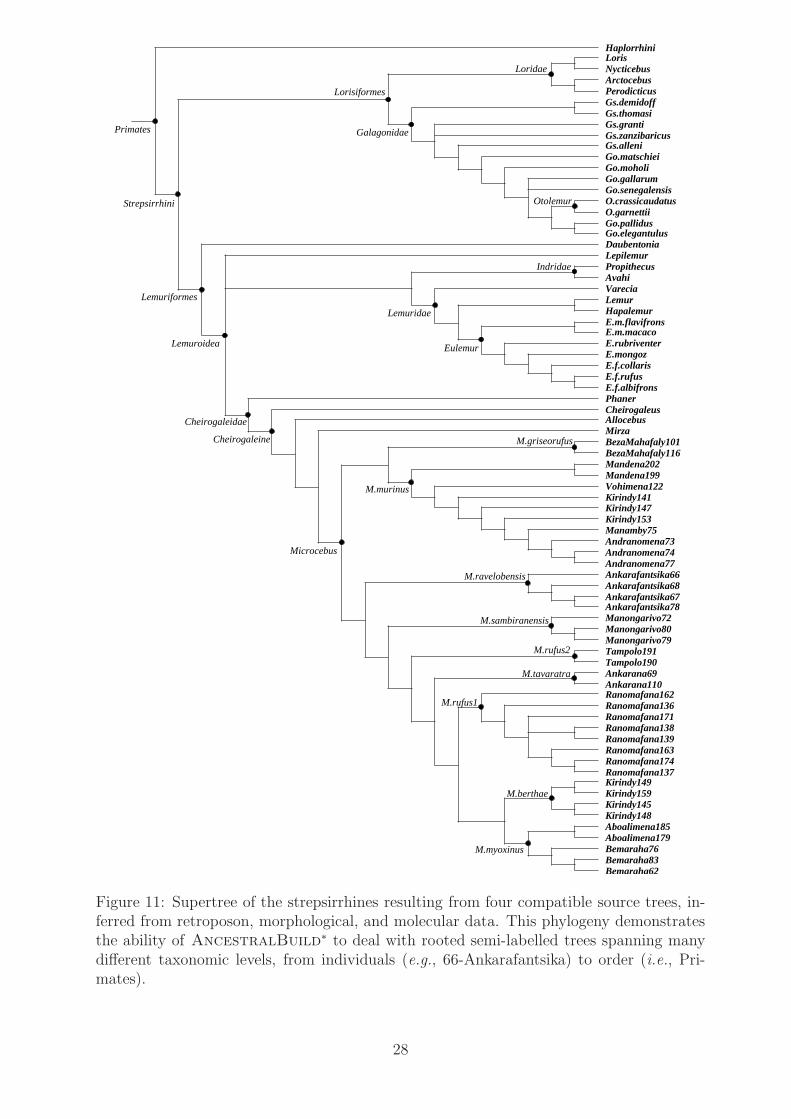
Internal labels of trees (b), (c), and (d) correspond to those displayed in the origi-nal figures, while those in tree (a) were added manually to demonstrate the ability ofAncestralBuild∗ to deal accurately with many labels, located at the same or differentlevels in the trees. The four detailed source trees are ancestrally compatible and Figure 11shows the supertree resulting from the application of AncestralBuild∗ to this collec-tion. The obtained phylogeny is one of the largest produced for the strepsirrhines, spanningapproximately 100 taxa on a number of taxonomic levels, from order to individuals. Thesource trees used in this example as well as the final supertree are accessible from theSystematic Biology web site.

Discussion

AncestralBuild∗ does not take primary data as input, but rather source trees inferredfrom this data with some level of confidence and through an adequate method. Thus,it is likely that the source trees considered for building a supertree will be more oftencompatible than, say, a set of primary character data. Nonetheless, it is likely that inmany cases the source trees turn out to be incompatible. Providing a faster way than othercurrent supertree methods to detect this incompatibility is a first goal of the algorithmpresented in this paper. However, this does not mark the end of its use in the process ofbuilding a supertree. Indeed,

(i) AncestralBuild∗ can be integrated in a general supertree method that builds asupertree by resolving incompatibilities in the source trees.

(ii) Moreover, AncestralBuild∗ as a whole can be used repeatedly to quickly identifycompatible subsets of the set of source trees or parts of the source trees that arecompatible. The resulting compatible subsets or parts are then combined into asupertree using AncestralBuild∗.

We indicate below some hints in both these directions.

27

Go.moholiGo.gallarumGo.senegalensisO.crassicaudatusO.garnettiiGo.pallidusGo.elegantulusDaubentoniaLepilemurPropithecusAvahiVareciaLemurHapalemurE.m.flavifronsE.m.macacoE.rubriventerE.mongozE.f.collarisE.f.rufusE.f.albifronsPhanerCheirogaleusAllocebusMirzaBezaMahafaly101BezaMahafaly116Mandena202Mandena199Vohimena122Kirindy141Kirindy147Kirindy153Manamby75Andranomena73Andranomena74Andranomena77Ankarafantsika66Ankarafantsika68Ankarafantsika67Ankarafantsika78Manongarivo72Manongarivo80Manongarivo79Tampolo191Tampolo190Ankarana69Ankarana110Ranomafana162Ranomafana136Ranomafana171Ranomafana138Ranomafana139Ranomafana163Ranomafana174Ranomafana137Kirindy149Kirindy159Kirindy145Kirindy148Aboalimena185Aboalimena179Bemaraha76Bemaraha83Bemaraha62

Go.matschiei

Primates

Strepsirrhini

Lorisiformes

Galagonidae

Indridae

Lemuridae

Eulemur

M.griseorufus

Lemuriformes

Lemuroidea

Cheirogaleidae

Cheirogaleine

M.murinus

Microcebus

M.ravelobensis

M.tavaratra

M.rufus2

M.sambiranensis

M.rufus1

M.berthae

M.myoxinus

Loridae

Otolemur

HaplorrhiniLorisNycticebusArctocebusPerodicticusGs.demidoffGs.thomasiGs.grantiGs.zanzibaricusGs.alleni

Figure 11: Supertree of the strepsirrhines resulting from four compatible source trees, in-ferred from retroposon, morphological, and molecular data. This phylogeny demonstratesthe ability of AncestralBuild∗ to deal with rooted semi-labelled trees spanning manydifferent taxonomic levels, from individuals (e.g., 66-Ankarafantsika) to order (i.e., Pri-mates).

28

Integration of AncestralBuild∗ in a general supertree method

As stated in the introduction, consistency is an attractive property for any supertreemethod. Thus, in constructing a general supertree method, deciding compatibility is anintegral part of the method. Currently, it seems that the only general supertree methods forrooted semi-labelled trees is given in Daniel and Semple (2005). In this paper, the authorsdescribe a general supertree method that allows for the possibility of variants. This method,called NestedSupertree, extends AncestralBuild, and thus AncestralBuild∗. Ifthe source trees are compatible, then it outputs a supertree that ancestrally displays eachof these trees. On the other hand, if the source trees are not compatible, then at someiteration there are no nodes that have indegree zero and no incident edges. By makingan appropriate choice of nodes to delete, NestedSupertree, or more particularly one ofits variants, resolves this and continues on, eventually returning a supertree with severaldesirable features including the following:

(i) ancestrally displaying every rooted binary semi-labelled trees that is ancestrally dis-played by each of the source trees;

(ii) independent of the order in which the source trees are listed.

We also remark that NestedSupertree runs in polynomial time and allows for the sourcetrees to be weighted. Such weights, irrelevant for deciding compatiblity (and thus ignoredby AncestralBuild), can really help to arbitrate the conflicts between incompatiblesource trees.

The progress made in this paper on the running time of AncestralBuild improvesthe practicality of general supertree methods for nested taxa such as NestedSupertree.

Repeated use of AncestralBuild∗ in the production of a supertree

Despite the exactness AncestralBuild∗, it can still be used to build a supertree fromincompatible source trees. Two ways are highlighted below.

• Finding a subset of the source trees that are compatible. Given an incom-patible collection P of source trees, finding a maximum-sized subset of trees in Pthat are compatible is an NP-hard task (Bryant, 1997). However, heuristic methodscan be easily implemented: (i) rank all trees in P according to their size, or to someconfidence value on the trees (e.g., bayesian posterior probabilities) or in the primarydata set from which they were obtained; (ii) build a compatible collection P ′ ⊆ Pin the following way: starting from the best ranked tree, consider each source treeof P successively and add it to P ′ if it forms a compatible collection with the trees

29

already in P ′, which is checked by AncestralBuild∗. At the end of the process,P ′ is a subset of compatible source trees, a supertree of which is provided by thefinal call to AncestralBuild∗.

• Finding parts of the source trees that are compatible. Usually, source treesresult from an extensive analysis of primary data and their clades are provided withassociated confidence values, such as bootstrap values or bayesian posterior proba-bilities. As a first approximation, we may assume that these confidence values arerepresentative in some sense of the correctness of the corresponding clades (see e.g.Berry and Gascuel (1996) for a discussion). Thus, when source trees are incompat-ible, a reasonable option is to first put into question the clades of the source treesthat display the least support from the data. This suggests an intuitive and simplescheme to remove conflicts from the source trees by collapsing some of the cladesfrom consideration: Let O be the list of support values for clades of the source trees,sorted by increasing order of confidence. Note that a clade appearing in differenttrees with different confidence values can be accounted for by resorting to suitableweighting schemes. Collapse clades of the source trees whose support value is equalto the first value of O and remove that value from the list. Then iterate until themodified source trees are compatible. Compatibility is checked every time by us-ing AncestralBuild∗, the final call providing a supertree from the collection ofmodified trees.

Acknowledgments

The authors are grateful to E. Douzery and P.-H. Fabre for indicating studies on thestrepsirrhine evolution used in this paper and for verifying our findings.

We thank Olaf Bininda-Emonds, Rod Page, Gabriel Valiente, and an anonymous refereefor their valuable comments. We expect the idea of Bininda-Emonds regarding a referencetaxonomy as additional input to play an important practical role in the use of supertreealgorithms.

The first author was supported by the Act. Incit. Inf.-Math.-Phys. en Biol. Mol.[ACI IMP-Bio] and the Act. Inter. Incit. Region. [BIOSTIC-LR]. The second authorwas supported by the New Zealand Marsden Fund and a University of Canterbury ErskineGrant. This work was done while the second author was a Visiting Professor at theUniversite of Montpellier II.

References

Aho, A. V., Y. Sagiv, T. G. Szymanski, and J. D. Ullman. 1981. Inferring a tree from lowestcommon ancestors with an application to the optimization of relational expressions.

30

SIAM J. Comput. 10:405–421.

Berry, V. and O. Gascuel. 1996. On the interpretation of bootstrap trees: appropriatethreshold of clade selection and induced gain. Mol. Biol. Evol. 13:999–1011.

Bininda-Emonds, O. R. P., ed. 2004. Phylogenetic supertrees: combining information toreveal the Tree of Life. Kluwer, Dordrecht.

Bininda-Emonds, O. R. P., K. E. Jones, S. A. Price, M. Cardillo, R. Grenyer, and A. Purvis.2004. Garbage in, grabage out. Pages 267–280 in Phylogenetic supertrees: combininginformation to reveal the Tree of Life (O. R. P. Bininda-Emonds, ed.). Kluwer, Dor-drecht.

Bordewich, M., G. Evans, and C. Semple. 2005. Extending the limits of supertree methods.Ann. of Comb. (in press) .

Bryant, D. 1997. Building trees, hunting for trees, and comparing trees: theory and meth-ods in phylogenetic analysis. Ph.D. thesis University of Canterbury.

Daniel, P. and C. Semple. 2004. Supertree algorithms for nested taxa. Pages 151–171 inPhylogenetic supertrees: combining information to reveal the Tree of Life (O. R. P.Bininda-Emonds, ed.). Kluwer, Dordrecht.

Daniel, P. and C. Semple. 2005. A class of general supertree methods for nested taxa.SIAM J. Discrete Math. (in press) .

Even, S. and Y. Shiloach. 1981. An on-line edge deletion problem. Journal of the Associa-tion of Computing Machinery 28:1–4.

Grunewald, S., M. Steel, and M. Swenson. 2005. Closure operations in phylogenetics. Tech.rep. University of Canterbury.

Henzinger, M. R., V. King, and T. Warnow. 1999. Constructing a tree from homeomorphicsubtrees, with applications to computational evolutionary biology. Algorithmica 24:1–13.

Hibbett, D., R. H. Nilsson, M. Snyder, M. F. andJ Costanzo, and M. Shonfeld. 2005.Automated phylogenetic taxonomy: an example in the homobasidiomycetes (mushroom-forming fungi). Syst.Biol. 54:660–668.

Holm, J., K. de Lichtenberg, and M. Thorup. 1998. Poly-logarithmic deterministic fully-dynamic algorithms for connectivity, minimum spanning tree, 2-edge, and biconnectivity.Pages 78–89 in Proceedings of the 30th Annual ACM Symp. on Theory of Computing.

Llabres, M., J. Rocha, F. Rossello, and G. Valiente. 2005. On the ancestral compatibilityof two phylogenetic trees with nested taxa. Submitted .

31

Masters, J. C. and D. J. Brothers. 2002. Lack of congruence between morphological andmolecular data in reconstructing the phylogeny of the galagonoidae. American Journalof Physical Anthropology 117:79–93.

Page, R. D. M. 2002. Modified mincut supertrees. Pages 537–552 in Second InternationalWorkshop on Algorithms in Bioinformatics (R. Guig and D. Gusfield, eds.) Springer.

Page, R. D. M. 2004. Taxonomy, supertrees, and the tree of life. Pages 247–265 in Phylo-genetic supertrees: combining information to reveal the Tree of Life (O. R. P. Bininda-Emonds, ed.). Kluwer, Dordrecht.

Page, R. D. M. and G. Valiente. 2005. An edit script for taxonomy classifications. BMCBioinformatics 6.

Roos, C., J. Schmitz, and H. Zischler. 2004. Primate jumping genes elucidates strepsirrhinephylogeny. Proceedings of the National Academy of Sciences 29:10650–10654.

Sanderson, M. J., B. G. Baldwin, G. Bharathan, C. S. Campbell, D. Ferguson, J. M.Porter, C. V. Dohlen, M. F. Wojciechowski, and M. J. Donoghue. 1993. The growth ofphylogenetic information and the need for a phylogenetic database. Syst. Biol. 42:562–568.

Semple, C. and M. Steel. 2000. A supertree method for rooted trees. Discrete Appl. Math.105:147–158.

Semple, C. and M. Steel. 2003. Phylogenetics. Oxford University Press, Oxford.

Yoder, A. D., R. M. Rasoloarison, S. M. Goodman, J. A. Irwin, S. Atsalis, M. J. Ravosa,and J. U. Ganzhorn. 2000. Remarkable species diversity in malagasy mouse lemurs (pri-mates, microcebus). Proceedings of the National Academy of Sciences 97:11325–11330.

Zaroliagis, C. D. 2002. Implementations and experimental studies of dynamic graph al-gorithms. Pages 229–278 in Experimental algorithms: from algorithm design to robustand efficient software vol. 2547 of Lect. Notes in Comput. Sci. Springer.

Appendix 1: Correctness of AncestralBuild∗

To ease reading in the following proofs, we view a node ℓ of a restricted descendancy graphthat is not a most recent common ancestor label as a single-element set. Theorem 8 followsfrom Proposition 4 and Lemma 12.

Lemma 11 Let P be a collection of rooted semi-labelled trees on X, and let P ′ be a col-lection of rooted fully-labelled trees that is obtained from P by adding most recent common

32

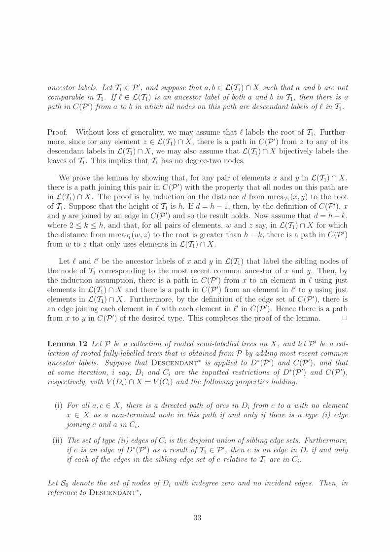
ancestor labels. Let T1 ∈ P′, and suppose that a, b ∈ L(T1) ∩X such that a and b are not

comparable in T1. If ℓ ∈ L(T1) is an ancestor label of both a and b in T1, then there is apath in C(P ′) from a to b in which all nodes on this path are descendant labels of ℓ in T1.

Proof. Without loss of generality, we may assume that ℓ labels the root of T1. Further-more, since for any element z ∈ L(T1) ∩X, there is a path in C(P ′) from z to any of itsdescendant labels in L(T1) ∩X, we may also assume that L(T1) ∩X bijectively labels theleaves of T1. This implies that T1 has no degree-two nodes.

We prove the lemma by showing that, for any pair of elements x and y in L(T1) ∩X,there is a path joining this pair in C(P ′) with the property that all nodes on this path arein L(T1) ∩ X. The proof is by induction on the distance d from mrcaT1

(x, y) to the rootof T1. Suppose that the height of T1 is h. If d = h− 1, then, by the definition of C(P ′), xand y are joined by an edge in C(P ′) and so the result holds. Now assume that d = h− k,where 2 ≤ k ≤ h, and that, for all pairs of elements, w and z say, in L(T1) ∩X for whichthe distance from mrcaT1

(w, z) to the root is greater than h− k, there is a path in C(P ′)from w to z that only uses elements in L(T1) ∩X.

Let ℓ and ℓ′ be the ancestor labels of x and y in L(T1) that label the sibling nodes ofthe node of T1 corresponding to the most recent common ancestor of x and y. Then, bythe induction assumption, there is a path in C(P ′) from x to an element in ℓ using justelements in L(T1) ∩X and there is a path in C(P ′) from an element in ℓ′ to y using justelements in L(T1) ∩ X. Furthermore, by the definition of the edge set of C(P ′), there isan edge joining each element in ℓ with each element in ℓ′ in C(P ′). Hence there is a pathfrom x to y in C(P ′) of the desired type. This completes the proof of the lemma. 2

Lemma 12 Let P be a collection of rooted semi-labelled trees on X, and let P ′ be a col-lection of rooted fully-labelled trees that is obtained from P by adding most recent commonancestor labels. Suppose that Descendant∗ is applied to D∗(P ′) and C(P ′), and thatat some iteration, i say, Di and Ci are the inputted restrictions of D∗(P ′) and C(P ′),respectively, with V (Di) ∩X = V (Ci) and the following properties holding:

(i) For all a, c ∈ X, there is a directed path of arcs in Di from c to a with no elementx ∈ X as a non-terminal node in this path if and only if there is a type (i) edgejoining c and a in Ci.

(ii) The set of type (ii) edges of Ci is the disjoint union of sibling edge sets. Furthermore,if e is an edge of D∗(P ′) as a result of T1 ∈ P

′, then e is an edge in Di if and onlyif each of the edges in the sibling edge set of e relative to T1 are in Ci.

Let S0 denote the set of nodes of Di with indegree zero and no incident edges. Then, inreference to Descendant∗,

33

(I) After Step 3′(a) is completed, if S1,S2, . . . ,Sk are the node sets of the arc componentsof Di\S0, then S1 ∩X,S2 ∩X, . . . ,Sk ∩X are the node sets of the blue componentsof Ci\(S0 ∩X).

(II) Before Step 3′(c) is performed, an edge e = {ℓ, ℓ′} of Di\S0 joins two arc componentsif and only if, for each sibling edge set of e, each edge in this set is coloured red andjoins two blue components in Ci\(S0 ∩X) with the labels in ℓ in one blue componentand the labels in ℓ′ in the other blue component.

(III) After Step 3′(c) is completed, for each arc component of Di\S0 and the correspondingblue component of Ci\(S0 ∩X), (i) and (ii) still hold.

Proof. We first prove (I). As every directed path in Di\S0 must end with an element ofX, it follows that, for all i, we have that Si ∩X is non-empty.

Let U be the node set of a blue component of Ci\(S0 ∩X). Let a and b be nodes in U ,and suppose that a and b are joined by a blue edge. Then either

(a) b is an ancestor of a or a is an ancestor of b in some tree in P, or

(b) {a, b} is an element of a sibling edge set of an edge, e say, in D(P ′).

Since Di and Ci satisfy (i), it follows that in case (a), there is either a directed path fromb to a or a directed path from a to b in Di\S0. In both cases, a and b are in the same arccomponent of Di\S0. If (b) holds, then, by (ii), e appears in Di\S0. Furthermore, as {a, b}is blue, the parent node of {a, b} in Di is not an element of S0. It follows that, in Di\S0,there is an arc from this parent node to one end of e and an arc from this parent node tothe other end of e. In particular, this means that a and b are in the same arc componentof Di\S0. It now follows that U is a subset of the node set of some component, Sj say, ofDi.

To complete the proof, we next show that Sj ∩X is not the (disjoint) union of the nodesets of two or more blue components of Ci\(S0∩X). To see this, assume that this happens.Then, in the arc component of Di\S0 whose node set is Sj, there is a path of arcs (notnecessarily a directed path) from a node c that is in the node set of one blue component ofCi\(S0∩X) to a node d that is in the node set of another blue component of Ci\(S0∩X).Without loss of generality, we may assume that amongst all such pairs of blue componentsin Ci\(S0 ∩X) and pairs of elements of X this path is of minimum length. By minimality,apart from c and d, there are no other elements of X on this path. But then each of thenon-terminal nodes on this path are elements in L(P ′) − X. Since each of these labelsacross all trees in P ′ are distinct, we deduce that each of these labels come from the sametree, T1 say, in P ′. If d is an ancestor of c or c is an ancestor of d in T1, it follows by theminimality condition that {c, d} is a blue edge in Ci\(S0 ∩X); a contradiction. So assume

34

that c and d are non-comparable in T1. By considering the directions of the arcs in thepath of directed edges between c and d, it is easily seen that one node on this path, ℓ say,is an ancestor label of both c and d in T1. Since the node ℓ appears in Di\S0, it followsby the fact that V (Di) ∩ X = V (Ci) that each of its descendant labels in L(T1) ∩X arein Ci\(S0 ∩ X). From Lemma 11, we now deduce that there is a path of blue edges inCi\(S0 ∩X) from c to d, and so c and d are in the same blue component of Ci\(S0 ∩X).This contradiction completes the proof of (I).

To prove (II), first suppose that before Step 3′(c) is performed e = {ℓ, ℓ′} is an edgeof Di\S0 joining two arc components. Then no parent node of any sibling edge set of e isin the node set of Di\S0 and so, if it exists, every edge in each of these sets is colouredred in Ci\(S0 ∩ X). Since {ℓ, ℓ′} is an edge of Di\S0, every element in ℓ ∪ ℓ′ is in thenode set of Ci\(S0 ∩X) and so, by (ii), we deduce that all such edges exist. Now considerthe elements in ℓ. If ℓ is a singleton, then, trivially, the labels in ℓ are in a single arccomponent. Therefore, assume that ℓ contains two labels x and y. Then ℓ corresponds tothe most recent common ancestor of x and y in some tree in P ′. It follows that x and yare in the same arc component of Di\S0. Applying the same arguments to ℓ′ and using(I), we deduce one direction of (II).

For the converse of (II), suppose that, for each sibling edge set of e, each of the edgesin this set are coloured red and join two blue components in Ci\(S0 ∩X) with the labelsin ℓ in one blue component and the labels in ℓ′ in the other blue component. Then it isimmediate from (I) that {ℓ, ℓ′} joins two arc components in Di\S0. This completes theproof of (II).

For (III), consider a component D of Di\S0 and the corresponding component, C say,of Ci\(S0∩X). First assume that there is a directed path of arcs in D from c to a with noelement x ∈ X as a non-terminal node. Then, as c 6∈ S0, we have that c and a are elementsof C. Since (i) holds for Di and Ci, it immediately follows there is an arc joining c and ain C. A similar argument shows that the converse also holds. Thus D and C satisfy (i).

Now consider (ii) in the statement of the lemma. First observe that, as the type (ii)edges of Ci is the disjoint union of sibling edge sets, it follows by (II) and the way in whichtype (ii) edges of Ci and edges of Di are deleted that the type (ii) edges of C is the disjointunion of sibling edge sets. Now assume that e is an edge in D with ends ℓ and ℓ′. Then,by the construction of D∗(P ′), it follows that ℓ∪ ℓ′ is a subset of the node set of D. As allof the elements in ℓ∪ ℓ′ are in X, we deduce by (I) that ℓ∪ ℓ′ is a subset of the node set ofC. Since (ii) holds for Di and Ci, it follows that each of the edges in the sibling edge setsof e are in C. A similar argument shows that the converse also holds. 2

35

Appendix 2: Implementation Details

We give here a description of AncestralBuild∗ that is more tuned towards implemen-tation. Data structures maintained throughout the algorithmic process are first detailed,then a pseudo-code details their precise interactions in the Descendant∗ subroutine.

Data structures

C(P ′) is a graph with node set X and whose edges can be one of two colours (blue orred). The nodes of C(P ′) are stored in an adjacency list. For each node v, we store itsblue neighbours (i.e., the nodes connected to v by a blue edge) in a doubly-linked list B(v)and its red neighbors in a doubly-linked list R(v). These neighbour relations code for theedges of C(P ′). Note that an edge {u, v} of a given color, say blue, is represented twice,because both u ∈ B(v) and v ∈ B(u).

D∗(P ′) is a mixed graph with node set L(P ′). For each node of D∗(P ′), we store itsindegree, its list of out-going arcs, and the list of nodes to which it is connected by an edge.For each node, we also maintain a list of pointers to the sibling edges of which it is parent.For each sibling edge of D∗(P ′), we also maintain a list of pointers to the corresponding(one to four) edges in C(P ′). This pointer is doubled so that these edges in C(P ′) knowin constant time their corresponding sibling edge in D∗(P ′). Thus, changing in C(P ′) thecolour of sibling edges {u, v} of a node x ∈ D∗(P ′) is done in constant time for each edge(recall that B(v), and similarily B(u), is a doubly-linked list, so that removing a pointedelement out of it and putting it in R(v) is done in constant time).

numC is a table indicating for each node s in C(P ′) the number of its current bluecomponent in C(P ′). Initially, all elements belong to the same component (without lossof generality, we may assume that C(P ′) is initially connected).

Comp is a table storing the blue components of C(P ′). Each component is coded as adoubly-linked lists of nodes of X and is stored in the entry of corresponding to its number.

S is a table, whose ith entry, Si, is the doubly-linked list of nodes of the ith arc compo-nent that have indegree 0 and no incident edge. If such a node of D∗(P ′) has a label in X,then there is a link between this node in Si and the corresponding node of C(P ′) storedin the list Compi which stores the nodes of the ith blue component. Thus, when a nodeof C(P ′) is moved from the ith blue component to the jth one (just created because of thedeletion of an edge), the corresponding node of D∗(P ′) moves from Si to Sj in constanttime.

LnextC is the list of new blue components in C(P ′) (corresponding to the new arc com-

ponents in D∗(P ′)) created during the on-going execution of Descendant∗.

36

A is the dynamic connectivity algorithm supporting deletion updates and connectivityqueries.

Pseudo-code for the Descendant∗ subroutine

The heading of the subroutine is the following:

Algorithm 1: Descendant∗ (D∗(P ′), C(P ′), n0)

Input: The descendancy graph D∗(P ′), the component graph C(P ′), and an arccomponent of D∗(P ′) to process indicated by its number n0.

Result: A tree with root labelled by Sn0∩X displaying a part of P ′, or the statement

no possible labelling

1 if Sn0is empty then return no possible labelling

2 if Cn0contains only one node v then

return the tree composed of one leaf with the label of v

First note that the whole graphs D∗(P ′) and C(P ′) are indicated as formal parameters,and not part of them. Indeed, to avoid unnecessary copies of parts of these graphs, it issimpler that all calls to the subroutine access the same shared data structure. Each callto the subroutine has to work on a single arc component of D∗(P ′) whose number n0 isinputted to the subroutine.

37

3′(a)(i) LnextC ← ∅ ; S∗

n0← ∅ ;

foreach s ∈ Sn0do

delete s and every incident arc (s, x) in D∗(P ′);if as a result, node x has indegree 0 (and no incident edge) then

S∗n0← S∗

n0∪ {x} /* for next call on this component */

3′(a)(ii) foreach s ∈ Sn0∩X do

remove s from CompnumC(s);foreach edge {s, x} ∈ C(P ′) do

delete {s, x} from C(P ′) and send to A the corresponding edge deletionupdate

3′(a)(iii) Lred ← ∅ /* list of edges coloured red in C(P ′) */;foreach s ∈ Sn0

do

let Sib(s) be the set of sibling edges whose parent is s;foreach e ∈ Sib(s) do

let L(ii)(e) be the sibling edge set of C(P ′) corresponding to e;colour red all edges of L(ii)(e) in C(P ′);Lred ← Lred ∪ L(ii)(e)

Sn0← S∗

n0;

Deleting nodes of Sn0from D∗(P ′) can lead to other nodes of the nth

0 arc componentto have indegree 0 (and no incident edge). However, these nodes are put aside (until theend of Step 3′(a)(iii)) in a list S∗

n0and not directly in S0 to avoid confusion between the

elements in that set at the beginning of the on-going call, and elements to be processed inthe next recursive call for the same arc component.

Also recall that removing nodes from C(P ′) at Step 3′(a)(ii) (namely, nodes in Sn0∩X)

does not change the set of blue components of the graph.

38

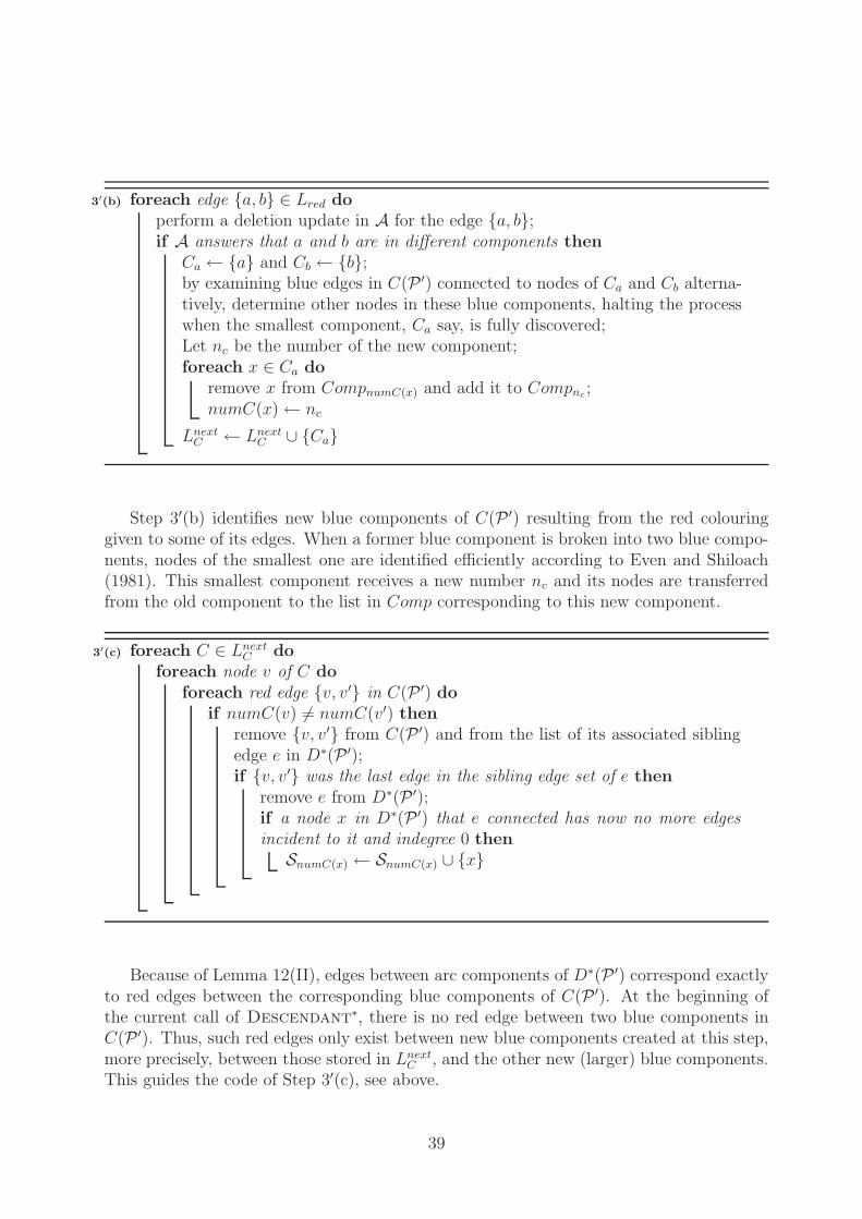
3′(b) foreach edge {a, b} ∈ Lred do

perform a deletion update in A for the edge {a, b};if A answers that a and b are in different components then

Ca ← {a} and Cb ← {b};by examining blue edges in C(P ′) connected to nodes of Ca and Cb alterna-tively, determine other nodes in these blue components, halting the processwhen the smallest component, Ca say, is fully discovered;Let nc be the number of the new component;foreach x ∈ Ca do

remove x from CompnumC(x) and add it to Compnc;

numC(x)← nc

LnextC ← Lnext

C ∪ {Ca}

Step 3′(b) identifies new blue components of C(P ′) resulting from the red colouringgiven to some of its edges. When a former blue component is broken into two blue compo-nents, nodes of the smallest one are identified efficiently according to Even and Shiloach(1981). This smallest component receives a new number nc and its nodes are transferredfrom the old component to the list in Comp corresponding to this new component.

3′(c) foreach C ∈ LnextC do

foreach node v of C do

foreach red edge {v, v′} in C(P ′) do

if numC(v) 6= numC(v′) then

remove {v, v′} from C(P ′) and from the list of its associated siblingedge e in D∗(P ′);if {v, v′} was the last edge in the sibling edge set of e then

remove e from D∗(P ′);if a node x in D∗(P ′) that e connected has now no more edgesincident to it and indegree 0 then

SnumC(x) ← SnumC(x) ∪ {x}

Because of Lemma 12(II), edges between arc components of D∗(P ′) correspond exactlyto red edges between the corresponding blue components of C(P ′). At the beginning ofthe current call of Descendant∗, there is no red edge between two blue components inC(P ′). Thus, such red edges only exist between new blue components created at this step,more precisely, between those stored in Lnext

C , and the other new (larger) blue components.This guides the code of Step 3′(c), see above.

39

4 foreach component Ci in LnextC ∪ {Cn0

} do

resi ← Descendant∗ (C(P ′), D∗(P ′), i);if resi returns no possible labelling then return no possible labelling

return the tree obtained by grafting all resi as child subtrees of a root node labelledby nodes in Sn0

∩X.

Note that, in the case where P ′ is compatible, Step 4 issues a recursive call for eachnew component created by the on-going execution of Descendant∗, as well as for thecomponent Cn0

. Indeed, this latter component still contains nodes. Note that some ofthese nodes that were not in Sn0

at the beginning of the on-going call, can now be inthis set because initial nodes of this set and some edges have been removed from this arccomponent.

40