Fast Automatic Heuristic Construction UsingActive Learning

William F. Ogilvie1, Pavlos Petoumenos1, Zheng Wang2, and Hugh Leather1

1 School of Informatics, University of Edinburgh, UK{s0198982, ppetoume, hleather}@inf.ed.ac.uk

2 School of Computing and Communications, Lancaster University, UKz.wang@lancaster.ac.uk

Abstract. Building effective optimization heuristics is a challengingtask which often takes developers several months if not years to com-plete. Predictive modelling has recently emerged as a promising solution,automatically constructing heuristics from training data. However, ob-taining this data can take months per platform. This is becoming an evermore critical problem and if no solution is found we shall be left without of date heuristics which cannot extract the best performance frommodern machines.In this work, we present a low-cost predictive modelling approach forautomatic heuristic construction which significantly reduces this train-ing overhead. Typically in supervised learning the training instances arerandomly selected to evaluate regardless of how much useful informationthey carry. This wastes effort on parts of the space that contribute lit-tle to the quality of the produced heuristic. Our approach, on the otherhand, uses active learning to select and only focus on the most usefultraining examples.We demonstrate this technique by automatically constructing a model todetermine on which device to execute four parallel programs at differingproblem dimensions for a representative Cpu–Gpu based heterogeneoussystem. Our methodology is remarkably simple and yet effective, makingit a strong candidate for wide adoption. At high levels of classificationaccuracy the average learning speed-up is 3x, as compared to the state-of-the-art.

Keywords: machine learning, workload scheduling

1 Introduction

Building effective program optimization heuristics is a daunting task becausemodern processors are complicated; they have a large number of components op-erating in parallel and each component is sensitive to the behaviour of the others.Creating analytical models on which optimization heuristics can be based hasbecome harder as processor complexity has increased, and this trend is bound tocontinue as processor designs move further towards heterogeneous parallelism [1].Compiler developers often have to spend months if not years to get a heuristic

right for a targeted architecture, and these days compilers often support a widerange of disparate processors. Whenever a new processor comes out, even ifderived from a previous one, the optimizing heuristics need to be re-tuned forit. This is typically too much effort and so, in fact, most compilers are out ofdate [2].

Machine Learning based predictive modelling has rapidly emerged as a vi-able means to automate heuristic construction; by running example programs(optimized in different ways) and observing how the variations affect programrun-time automatic machine learning tools can predict good settings with whichto compile new, as yet unseen, programs. There are many studies showing thatmachine learning outperforms human based approaches [2, 3]. Recent work alsoillustrates that it can be used to automatically port across architecture spaces [4]and can find more appropriate ways of mapping program parallelism to variousplatforms [5]. This new research area is promising, having the potential to fun-damentally change the way compiler heuristics are designed; that is to say, com-pilers can be automatically tuned for new hardware without the need for monthsof compiler experts’ time; however, before the potential of predictive modellingbased heuristic construction can be realized there remain many hurdles whichmust be tackled. One major concern is the cost of collecting training examples.While machine learning allows us to automatically construct heuristics with lit-tle human involvement, the cost of generating training examples (that allow alearning algorithm to accumulate knowledge) is often very expensive.

This paper presents a novel, low-cost predictive modelling approach that cansignificantly reduce the overhead of collecting training examples without sacrific-ing prediction accuracy. Traditionally in predictive modelling training examplesare randomly selected for labelling where, in the context of machine learningbased compilers and run-time systems, labelling involves profiling code undervarying conditions. This is inefficient because random selection often providesredundant data to the learner. In effect a cost is paid for training but little or nobenefit is actually received. We tackle this problem by using active learning [6]to select and only focus on useful training instances, which greatly reduces thetraining overhead. Specifically, we build a number of initial distinct models witha small set of randomly selected training examples. We ask those models to makepredictions on unseen data points, and the points for which the models ‘disagree’the most are profiled. We then rebuild the models by re-running the learningalgorithm with the new training example together with the existing ones, andrepeat this process until a completion criterion is met after which a final heuristicis produced. In this way, we profile and collect training examples that providethe most information to the algorithm, thereby enabling it to improve predictionaccuracy of the learned models more quickly.

We demonstrate the effectiveness of our approach by using active learning toautomatically construct a heuristic to determine which processor will give thebetter performance on a Cpu–Gpu based heterogeneous platform at differingproblem sizes for a given program. More specifically, our approach is evaluatedby building heuristics to predict the better processor to use for 4 benchmarks

which have equivalent OpenMp and OpenCl implementations; where OpenMpis used for the Cpu since it has a more mature implementation than OpenCl.Comparing our work to a typical random sampling technique, widely used inprior work, reveals that our methodology speeds up training by a factor of 3xon average: saving weeks of intensive compute time.

The research presented in this paper makes the following contributions. It

– shows that the training overhead of machine learning based compiler heuris-tics design can be significantly reduced without sacrificing prediction accu-racy;

– demonstrates how active learning can be used to automatically derive aheuristic to map OpenMp and OpenCl programs on a Cpu–Gpu basedheterogeneous platform;

– provides detailed analysis of active learning based heuristic tuning.

The rest of this paper is organized as follows: in Sect. 2 we give a motivatingexample for this research, in Sect. 3 we discuss our approach and the imple-mentation details of our system, in Sect. 4 we outline the methodology used tovalidate our technique, Sect. 5 provides our results and accompanying analysis,Sect. 6 references related work, and we conclude in Sect. 7.

2 Motivation

To motivate our work, we demonstrate how much unnecessary effort is involvedin the traditional random-sampling based learning techniques, and point out theextent to which a better strategy can improve matters. In Fig. 1(a) we show forHotSpot, from the Rodinia [7,8] suite, when it is better to run on the Cpu versusthe Gpu for maximum performance. The benchmark accepts two independentprogram inputs, and these form the axes of the graph. The graph data itselfwas generated by randomly selecting 12,000 input combinations and runningthem on both the Cpu and Gpu enough times to make a statistically sounddecision about which device is better for each, where a boundary line separatesthe regions at which either device should be chosen.

Machine learning has been shown to be a viable option for creating heuristicsfor this type of problem [9, 10]. To build such a heuristic, a machine learningalgorithm typically requires a set of training examples to learn from. In ourcase, we need to use a set of profiled program inputs to find a model that is agood estimate of the boundary as shown in Fig. 1(a). The quality of the trainingexamples will have a significant impact on the accuracy of the resultant model.

In Fig. 1(b) a random selection of 200 inputs to HotSpot is chosen, as mightbe typical in a standard ‘passive’ learning technique3. From this data a heuris-tic is created with the RandomCommittee machine learning algorithm from the

3 In passive learning techniques, the training examples are selected without feedback asto the quality of the machine learned heuristic. Most usually, this will mean that alltraining examples are generated ahead of time and then a heuristic is learned once.In active learning, by contrast, the selection of training examples is an iterativeprocess which is driven by feedback about the quality of the heuristic.

0 10 20 30 40 50 60 70 80 90 100 110 120 1300

20

40

60

80

100

120

CPU GPU

Pro

gra

m Inp

ut

Para

mete

r

Program Input Parameter

(a) The problem space

0 10 20 30 40 50 60 70 80 90 100 110 120 1300

20

40

60

80

100

120

Program Input Parameter

Pro

gra

m Inp

ut

Para

mete

r

CPU GPU Sample Points

(b) Random sample points

0 10 20 30 40 50 60 70 80 90 100 110 120 1300

20

40

60

80

100

120

Program Input Parameter

Pro

gra

m Inp

ut

Para

mete

r

CPU GPU Sample Points

(c) Ideal sample points

Fig. 1: Passive learning over randomly selected inputs versus learning from ideallyselected inputs. Figure (a) shows the problem space of the Rodinia HotSpot benchmark.12,000, 2-dimensional program inputs are run to discover which device (Cpu or Gpu)gives the better performance. A boundary line separates the parts of the space whereCpu and Gpu are better. Figure (b) shows a random selection of 200 inputs. UsingRandomCommittee to learn a heuristic with these inputs achieves an accuracy of 95%.Figure (c) shows an ideal selection of 50 inputs near to the boundary line. UsingRandomCommittee to learn a heuristic with these inputs achieves an accuracy of 97%,representing a 4x speed-up in training time.

Weka tool-kit [11], and the heuristic achieves a respectable 95% accuracy. Ma-chine learning can clearly learn good heuristics in this case, but our intuitioninsists that the majority of the randomly selected inputs offer little useful infor-mation. In fact, we would expect that only those points near to the boundaryline in Fig. 1(a) should be required to accurately define a model.

We prove this intuition in Fig. 1(c) where we have instead selected just 50inputs close to the boundary line and once again asked the RandomCommitteealgorithm to learn a heuristic. Using fewer than 15% as many observations asthe standard passive learning technique we achieve an accuracy of 97%. There is,therefore, significant potential to reduce the training cost for the machine learnedheuristics if we could only choose the right inputs to train over. Unfortunately,without already knowing the shape of the space it is impossible to tell whatthe best inputs should be, but nevertheless we will show that it is possible toapproximate their location.

In this paper we present a simple active learning technique that maintains aset of training inputs, adding to the set incrementally by selecting inputs thatlook likely to improve the heuristic quality based on what has already been seen.For the HotSpot benchmark, our approach avoids nearly all of the unimportantinputs, quickly focussing in on the best inputs to choose. Our active learningmethod needs only 31 inputs to create heuristics as accurate as passive learninggenerates with 200 inputs; a reduction in training cost of 85%. The followingsection describes our methodology in detail.

LearningAlgorithms

NewSamplePoints

InitialTrainingPoints

Active Learner

IntermediateModel

IntermediateModel

Final

Model

Fig. 2: An overview of our active learning approach. Initially, we use a few random

samples to construct several intermediate models. Those models are utilized to choose

which new data point is to be profiled. The new sampled data point is then used to

update the models. We repeat this process until a certain termination criterion is met

where a final model will be produced as the outcome.

3 Our Approach

As a case study, this work aims to learn a predictor to determine the bestprocessor to use for a given program input. We wish to avoid profiling inputsthat provide little or no information for the learning algorithm to train over sothat we can minimize the overhead of collecting training examples. We achievethis by using active learning which carefully chooses each input to be profiledin turn. At each step, our algorithm attempts to choose a new input that willmost improve the machine learned heuristic when it is added to the training setof examples.

Figure 2 provides an overview of how our approach can be applied to thiscase study problem. First, some number of program inputs are chosen at randomto ‘seed’ the algorithm and these are then profiled to determine the better devicefor them – Cpu or Gpu. What follows is a number of steps which progressivelyadd to the set of training inputs until some termination criterion are met. Toselect which program input to add to the training set for profiling, a numberof different, intermediate models are created using the current training set anddifferent machine learning algorithms. Our method then searches for an inputfor which the intermediate models or heuristics most disagree as to whether itshould be run on the Cpu or the Gpu. The intuition is that the more thesemodels agree on an input, the less likely it is able to improve the predictionaccuracy of the learned heuristic.

The technique for choosing new training inputs is called Query by Com-mittee (Qbc) [12] and is described in Sect. 3.1, whilst Sect. 3.3 details howthe program training inputs are profiled: particularly, how the decision aboutwhether the input should be run on the Cpu or on the Gpu is made statisticallysound.

3.1 Query by Committee

The key idea behind active learning is that a machine learning algorithm canperform better with fewer training points if it is allowed to choose the data fromwhich it learns. There are a number of approaches available [13] but we employ

a heterogeneous implementation of the Query by Committee (Qbc) algorithm,a widely utilized active learning technique, to select the most useful trainingexamples from the input-space.

The Qbc algorithm requires a group of distinct machine learning models (in-stead of just one) to be used. The ‘committee’ consists of a number of differentlearning algorithms that are initially trained with a small set of randomly col-lected training examples. In our case, those training examples are a set of profiledprogram inputs with a label indicating which processor gives better performancefor each input. As those models are initially built from a small set of trainingexamples, they are unlikely to be highly accurate. We will improve them withthe following iterative steps using new training examples. The key point is howto only select the training examples (i.e. which program inputs to be profiled inour case) that are likely to improve the prediction accuracy. To do so, we askeach model in the committee to make predictions on a random candidate set ofprogram inputs that are not present in the current training example set (andhence they haven’t been profiled yet). As a result, different models may or maynot reach consent for a particular program input. We then only profile thoseinputs for which the ‘committee’ disagrees the most to discover the true, best-performing processor, adding those new training examples into the training set,and re-running the learning algorithms to update the models. The justificationfor this is that we do not want to create new training instances from parts of theproblem-space which are already understood by the committee of algorithms,but rather would like to sample those regions which are least well defined. Theinsight being that if we reduce the regions of disagreement between the com-mittee members, by choosing training instances from within those regions, weincrementally get closer to the true boundary over which the processor choiceshould be altered and hence increase the accuracy of our final heuristic.

An Example: Figure 3 provides a hypothetical example to demonstrate hownew training points are selected by Qbc in our case. In Fig. 3(a) we are presentedwith an input-space which is fully described by two input parameters and hassome training samples already shown. In this example, our committee consistsof two different classification algorithms which will result in two classifiers thatwe will call X and Y. Based upon the location of these training examples in thespace, and which device is faster under these conditions (represented by differentshapes), the two different algorithms may give different models as illustrated inFig. 3(a) and Fig. 3(b). If we overlap these classification boundaries of the twomodels, as in Fig. 3(c), we can see that there are parts of the space that classifiersX and Y are in agreement about and a region of disagreement. Knowing thedisagreement regions, we then only select a new program input that both modeldisagree with to be profiled as our new training example. The question is whichprogram input to choose? This will certainly require a metric to access thedisagreement, which will be described in the next section.

Inpu

t Par

amet

er

Input Parameter

(a) Classifier X

Inpu

t Par

amet

er

Input Parameter

(b) Classifier Y

Inpu

t Par

amet

er

Input Parameter

Disagreement Area

(c) Disagreement betweentwo classifiers

Fig. 3: A simplified input space with two input parameters and the locations of profiled

training examples. We use two different learning algorithms to build two different

classifiers – (a) and (b). We then combine these models, as in (c), to find the region

of disagreement between them and use this information to better choose where future

training samples should be drawn from.

3.2 Assessing Disagreement

We use information entropy (1) [14] to evaluate the level of disagreement foreach point that have not been profiled so far, where p (xi) is the proportion ofcommittee members that predict that instance X is fastest on device i of n.The candidates with the maximum entropy value seen in each iteration of thelearning loop are collected and a random candidate is chosen from within thishigh entropy subset as the next training example. This means that the inputsassociated with the chosen candidate are run on the Cpu and Gpu kernels andit is determined which processor is faster under those input conditions. Thisnew training example is added to the current training set and its inputs areremoved form the candidate set to ensure the two remain disjoint. The learningloop begins another iteration with the models being formed with the addition ofthe new data.

H (X) = −n∑

i=1

p(xi) log p(xi) (1)

3.3 Statistical Sounded Profiling

Since computer timings are inherently noisy we use statistics to increase thereliability of our models. In particular, we record a minimum number of timingsfrom each device, as specified by the user. We use Interquartile Range [15] outlierremoval then apply Welch’s t-test [16] to discover if one hardware device is indeedfaster than the other. If we cannot conclude from the t-test that this is the case,then we perform an equivalence test. Both devices are said to be ‘equivalent’ ifthe difference between the higher mean plus its 95% confidence interval minusthe lower mean minus its confidence is within some threshold of indifference. In

our system this threshold was set to be within 1% of the minimum of the twomeans. If the fastest device cannot be determined and they are not equivalent anextra set of observations are obtained and the tests applied again, up until someuser defined number of tries. In the case of equivalence or of no determinationbeing made within this threshold of attempts the Cpu is chosen as the preferreddevice since it is more energy-efficient.

4 Experimental Setup

This section describes the details of the experimental case studies that we un-dertook, starting with the platform and benchmarks used, moving on to theparticular Qbc settings, and finally discussing the evaluation methodology.

4.1 Platform and Benchmarks

We evaluated our approach on a Cpu–Gpu based heterogeneous platform witha Intel Core i7 7770 4-core CPU (8 Hardware threads) @ 3.4GHz and a NVIDIAGeforce GTX Titan GPU (6 GB memory). The machine runs OpenSuse V12.3Linux and we use gcc V4.7.2 and the NVIDIA CUDA Toolkit v5.5 for compila-tion. We used 3 benchmarks from the Rodinia suite, HotSpot, PathFinder, andSRAD, and we also included a simple matrix multiplication application. Thesebenchmarks were specifically chosen because they had equivalent OpenCl andOpenMp versions and each has multiple program inputs which affect the di-mensions of their respective problem-spaces.

Table 1: The sizes of the input-space for each benchmark. Each dimension has a

value of between Min and Max, inclusive, and a step value of Stride. Size gives the

total number of points in each input-space, and Cand is the number of points in the

candidate set for each benchmark.

Benchmark #Dimentions Min Max Stride Size Cand

HotSpot 2 1 128 1 16, 384 10,000

MatMul 3 1 256 1 1.6x107 10,000

Pathfinder 2 2 1024 1 1.0x106 10,000

SRAD 2 128 1024 16 3, 136 2,636

4.2 Active Learning Settings

Machine Learning Models: Our active learning framework uses 12 unique algo-rithms from the Weka tool-kit to form the committee, each executed with de-fault parameter values. They are Logistic, MultilayerPerceptron, IB1, IBk,KStar, LogitBoost, MultiClassClassifier, RandomCommittee, NNge, ADTree,RandomForest, and RandomTree. These were selected because they can producea binary predictor from numeric inputs and have been widely used in prior work.

Program Input Space: The dimensions of the input-space for each benchmarkwere chosen to give realistic values to learn over – see Table 1.

Initial Training Set and Candidate Set Sizes: For all experiments the training setwas initialised with a single randomly chosen instance – the minimum possible.The effect of changing this parameter is discussed in Sect. 5.3. The candidateset size was either 10,000 inputs not already present in the training and test setsor the maximum number of points not in the training and test sets, whicheverwas smaller – see Table 1.

Termination Criterion: The learning iterations were halted at 200 steps since itwas found experimentally that the learning improvement had plateaued by thattime.

4.3 Evaluation Methodology

Runtime Measurement and Device Comparison To determine if a benchmarkis better suited to the Cpu or Gpu for a given input it is run on each deviceat least 10 times and at most 200 times. As mentioned in Sect. 3, we employinterquartile-range outlier removal, Welch’s t-test, and equivalence testing toensure the statistical soundness of the gathered program execution times.

Testing For testing purposes, a set of 500 inputs were excluded from any trainingand candidate sets. Both our active and passive learning experiments were run10 times for each benchmark and the arithmetic mean of the accuracy (or othermetrics) were recorded. For both active and passive learning, the accuracy wastaken as the average accuracy of all 12 models. That is to say, we comparedthe average accuracy achieved using a 12-member Qbc algorithm versus thesame 12 algorithms trained using random data as the number of Qbc-chosen orrandomly-chosen training sets increased in size.

5 Experimental Results

In this section we begin by presenting the overall results of our experiments,showing that our active learning approach can significantly reduce the trainingtime by a factor of 3 when compared to the random sampling technique. We thenmove on to examine the performance exhibited by our system for each benchmarkin turn. Finally, we discuss how the change in two user supplied parameters(i.e. initial training set and candidate set sizes) can affect the performance ofour methodology.

5.1 Overall Learning Costs

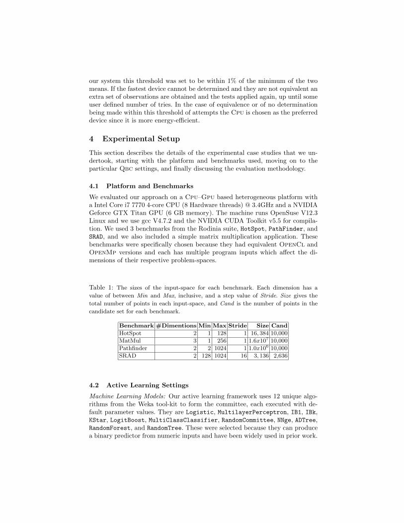
Figure 4 shows the average learning speed-up of our approach over the pas-sive, random-sampling technique traditionally used in heuristic construction.

hotspot matrix mult pathfinder srad geo. meansp

eedu

p

0

2

4

6

8

10

Fig. 4: On average our methodology requires 3x fewer training examples to create a

high quality heuristic than the traditional random-sampling technique, proving that

this simple algorithm can save weeks, and potentially months, of compute time.

The speed-up values are based on the number of inputs which need to be profiledin order to train a predictor to an accuracy of at least 85%. As can be seen fromthis figure, our approach constantly outperforms the classical random-samplingtechnique for all benchmarks, which in real terms means a saving of weeks totrain these heuristics.

5.2 Analysis of Training Point Selection

If we look at Figs. 5–8 we can see clearly where the cost savings associated withQbc are coming from. That is, in all cases the algorithm quickly chooses pointssurrounding the boundary between the Cpu and the Gpu optimum regions,giving it the ability to more accurately approximate its shape in less time.

5.3 Sensitivity to Parameters

As well as confirming the validity of our approach we also conducted two furtherexperiments to determine the impact that some user defined parameters mighthave on the effectiveness of the system. The first experiment involved alteringhow many randomly selected training examples were initially supplied to theQbc algorithm to get it started. The second experiment investigated the extentto which changing the candidate set size would have an effect on the speed ofheuristic construction. Results for both examinations are shown in Fig. 9 andFig. 10, respectively.

In Fig. 9 it is clear that increasing the number of random training instancesused to seed the Qbc algorithm for HotSpot has no significant affect in thelong-term performance but is detrimental in the short term, however, one canimagine a case where a complex space with many localized features may be betterexplored through an initially random approach followed-up by active learning.

Figure 10 shows how changing the size of the candidate set for the HotSpot

benchmark affects the performance of the system. In particular, the data in-dicates a lower candidate set size may be more beneficial. Presumably this isbecause a high candidate set increases the likelihood or the learner receivingredundant information from neighbouring high entropy points.

input parameter #1

inpu

t par

amet

er #

2

50 100 150 200 2500

50

100

150

200

250

CPU GPU

(a) Random Selection

input parameter #1

inpu

t par

amet

er #

2

100 150 200 250

100

150

200

250

CPU GPU

(b) Qbc Selection

Fig. 5: Since the Matrix Multiplication input-space is three-dimensional and not as

simply defined as the other benchmarks it is difficult for a human to visualise the

separation between Cpu and Gpu regions; to make it a little easier the graph above

was flattened so that the z-axis has values 122 ≤ z ≤ 144. However, active learning

was over six times faster than random sampling at producing a high quality model

for this code, quicker than the other programs tested and likely due to the additional

dimension reducing the effectiveness of random selection.

input parameter #1

inpu

t par

amet

er #

2

0 20 40 60 80 100 1200

20

40

60

80

100

120

CPU GPU

(a) Random Selection

input parameter #1

inpu

t par

amet

er #

2

0 20 40 60 80 100 1200

20

40

60

80

100

120

CPU GPU

(b) Qbc Selection

Fig. 6: The difference between Qbc and random sampling is stark for the HotSpot code.

In particular, the Qbc algorithm is able to quickly converge and define the boundary

between the two devices whilst random selection trains on redundant or less informative

points, proved by the fact it takes twice as long as Qbc.

6 Related Work

Analytic Modelling Analytic models have been widely used to tackle complexoptimization problems, such as auto-parallelization [17, 18], runtime estima-tion [19–21], and task mappings [22]. A particular problem with them, however,is the model has to be re-tuned whenever it is targeted at new hardware [23].

input parameter #1

inpu

t par

amet

er #

2

0 200 400 600 800 10000

200

400

600

800

1000

CPU GPU

(a) Random Selection

input parameter #1

inpu

t par

amet

er #

2

0 200 400 600 800 10000

200

400

600

800

1000

CPU GPU

(b) Qbc Selection

Fig. 7: The PathFinder Qbc graph displays more randomness than the previous two.

The probable reason for this, judging by the location of the boundary line, is that the

active learner cannot initially locate the Gpu region. Nevertheless, active learning is

still twice as fast at generating a good quality heuristic compared with the random

sampling technique.

input parameter #1

inpu

t par

amet

er #

2

200 400 600 800 1000

200

400

600

800

1000

CPU GPU

(a) Random Selection

input parameter #1

inpu

t par

amet

er #

2

200 400 600 800 1000

200

400

600

800

1000

CPU GPU

(b) Qbc Selection

Fig. 8: Similarly, the SRAD input-space appears to show that Qbc initially searches

randomly because it has difficulty approximating the location of the comparitively

small Cpu region. However, once the algorithm has an idea of where this region is

located it quickly concentrates on the boundary and forms a high-quality heuristic in

half the time of the passive learning methodology.

Predictive Modeling Predictive modeling has been shown to be useful in theoptimization of both sequential and parallel programs [9,10,24,25]. Its great ad-vantage is that it can adapt to changing platforms as it has no a priori assump-tions about their behaviour but it is expensive to train. There are many studiesshowing it outperforms human based approaches [2,3,26–29]. Prior work for ma-chine learning in compilers, as being exemplified by MilePost GCC project [30],often uses random sampling or exhaustive search to collect training examples.The process of collecting training examples could be expensive, taking several

training instances

accu

racy

%

0 50 100 150 20060

70

80

90

100

init. training set = 1init. training set = 4init. training set = 16init. training set = 64

Fig. 9: This graph shows that increasing the number of random examples given initially

to the Qbc algorithm for HotSpot is at first detrimental to its performance, however,

in a complex space increased randomness may help discover complex localized features.

training instances

accu

racy

%

0 50 100 150 20060

70

80

90

100

cand. set = 100cand. set = 1Kcand. set = 10Kcand. set = 40K

Fig. 10: This graph shows that choosing a lower candidate set size may be more ben-

eficial than a larger one.

weeks if not months. Using active learning, our approach can significantly re-duce overhead of collecting training examples. This accelerates the process oftuning optimization heuristics using machine learning. The Qilin compiler [31]uses runtime profiling to predict a parallel program’s execution time and mapwork across the CPU and GPU accordingly. Our approach does not requirerun-time profiling and therefore avoids program slow-downs resulted from thepotentially expensive runtime profiling.

Active Learning for Systems Optimization A recent paper by Zuluaga et al. [32]proposed an active learning algorithm to select parameters in a multi-objectiveproblem. Their work is not concerned with single-objective workload schedulingand does not consider statistical soundness of raw data. Balaprakash et al. [33,34]used active learning to reduce execution time of scientific codes but they onlyconsider code variants and OpenCl parameters as inputs; they do not discussthe impact of problem size on performance.

Problem Size Optimization Optimizing code for different problem sizes in hetero-geneous systems is discussed by Liu et al. [35] where they give an implementationof a compiler which uses a combination of regression trees and representativeGpu kernels, but their approach uses exhaustive search. Adaptic is a compila-tion system for Gpus [36] and uses analytical models to map an input streamonto the Gpu at runtime but their technique is not easily portable, where ourstackles that problem directly by making learning cheaper.

7 Conclusions

We have presented a novel, low-cost predictive modelling approach for machinelearning based automatic heuristic construction. Instead of building heuristicsbased on randomly chosen training examples we use active learning to focuson those instances that improve the quality of the resultant models the most.Using Qbc to construct a heuristic to predict which processor to use for a givenprogram input our approach speeds up training by a factor of 3x, saving weeksof compute time.

8 Acknowledgements

This work was funded under the EPSRC grant, ALEA (EP/H044752/1).

References

[1] J. Power, A. Basu, J. Gu, S. Puthoor, B. M. Beckmann, M. D. Hill, S. K. Rein-hardt, and D. A. Wood, “Heterogeneous System Coherence for Integrated CPU–GPU Systems,” in Proc. MICRO’13.

[2] S. Kulkarni and J. Cavazos, “Mitigating the Compiler Optimization Phase-Ordering Problem using Machine Learning,” in Proc. OOPSLA’12.

[3] C. Dubach, T. Jones, E. Bonilla, G. Fursin, and M. F. P. O’Boyle, “PortableCompiler Optimisation Across Embedded Programs and Microarchitectures usingMachine Learning,” in Proc. MICRO’09).

[4] J. Cavazos, G. Fursin, F. Agakov, E. Bonilla, M. F. P. O’Boyle, and O. Temam,“Rapidly Selecting Good Compiler Optimizations using Performance Counters,”in Proc. CGO’07.

[5] D. Grewe, Z. Wang, and M. F. O’Boyle, “Portable Mapping of Data ParallelPrograms to OpenCL for Heterogeneous Systems,” in Proc. CGO’13.

[6] B. Settles, “Active Learning Literature Survey,” University of Wisconsin–Madison, Computer Sciences Technical Report 1648, 2009.

[7] S. Che, M. Boyer, J. Meng, D. Tarjan, J. Sheaffer, S.-H. Lee, and K. Skadron,“Rodinia: A Benchmark Suite for Heterogeneous Computing,” in Proc. IISWC’09.

[8] S. Che, J. Sheaffer, M. Boyer, L. Szafaryn, L. Wang, and K. Skadron, “A Char-acterization of the Rodinia Benchmark Suite with Comparison to ContemporaryCMP Workloads,” in Proc. IISWC’10.

[9] K. D. Cooper, P. J. Schielke, and D. Subramanian, “Optimizing for Reduced CodeSpace using Genetic Algorithms,” in Proc. LCTES’99.

[10] Z. Wang and M. F. O’Boyle, “Mapping Parallelism to Multi-cores: A MachineLearning Based Approach,” in Proc. PPoPP’09.

[11] M. Hall, E. Frank, G. Holmes, B. Pfahringer, P. Reutemann, and I. H. Witten,“The WEKA Data Mining Software: An Update,” SIGKDD Explorations, 2009.

[12] H. S. Seung, M. Opper, and H. Sompolinsky, “Query by Committee,” inProc. COLT’92.

[13] C. M. Bishop, Pattern Recognition and Machine Learning (Information Scienceand Statistics). Springer-Verlag New York, Inc., 2006.

[14] I. Dagan and S. P. Engelson, “Committee-Based Sampling For Training Proba-bilistic Classifiers,” in Proc. ICML’95.

[15] D. S. Moore and G. P. McCabe, Introduction to the Practice of Statistics. W.H. Freeman, 2002.

[16] B. L. Welch, “The Generalization of “Student’s” Problem when Several DifferentPopulation Variances are Involved,” Biometrika, 1947.

[17] C. Bastoul, “Code Generation in the Polyhedral Model Is Easier Than YouThink,” in Proc. PACT’04.

[18] L.-N. Pouchet, C. Bastoul, A. Cohen, and J. Cavazos, “Iterative Optimization inthe Polyhedral Model: Part II, Multidimensional Time,” in Proc. PLDI’08.

[19] M. Clement and M. Quinn, “Analytical Performance Prediction on Multicomput-ers,” in Proc. SC’93.

[20] R. Wilhelm, J. Engblom, A. Ermedahl, N. Holsti, S. Thesing, D. Whal-ley, G. Bernat, C. Ferdinand, R. Heckmann, T. Mitra, F. Mueller, I. Puaut,P. Puschner, J. Staschulat, and P. Stenstrom, “The worst-case execution-timeproblem – overview of methods and survey of tools,” ACM TECS, 2008.

[21] S. Hong and H. Kim, “An Analytical Model for a GPU Architecture with Memory-level and Thread–level Parallelism Awareness,” in Proc. ISCA’09.

[22] A. H. Hormati, Y. Choi, M. Kudlur, R. Rabbah, T. Mudge, and S. Mahlke, “Flex-tream: Adaptive Compilation of Streaming Applications for Heterogeneous Archi-tectures,” in Proc. PACT’09.

[23] M. Stephenson, S. Amarasinghe, M. Martin, and U.-M. O’Reilly, “Meta Optimiza-tion: Improving Compiler Heuristics with Machine Learning,” in Proc. PLDI’03.

[24] Z. Wang and M. F. O’Boyle, “Partitioning streaming parallelism for multi-cores:a machine learning based approach,” in PACT ’10.

[25] D. Grewe, Z. Wang, and M. F. O’Boyle, “Opencl task partitioning in the presenceof gpu contention,” in LCPC ’13.

[26] D. Grewe, Z. Wang, and M. O’Boyle, “A workload-aware mapping approach fordata-parallel programs,” in HiPEAC ’11.

[27] M. Zuluaga, A. Krause, P. Milder, and M. Puschel, ““Smart” Design Space Sam-pling to Predict Pareto–Optimal Solutions,” in Proc. LCTES’12.

[28] M. K. Emani, Z. Wang, and M. F. P. O’Boyle, “Smart, adaptive mapping ofparallelism in the presence of external workload,” in CGO ’13.

[29] Z. Wang and M. F. P. O’boyle, “Using machine learning to partition streamingprograms,” ACM TACO, 2013.

[30] G. Fursin, C. Miranda, O. Temam, M. Namolaru, E. Yom-Tov, A. Zaks,B. Mendelson, E. Bonilla, J. Thomson, H. Leather, C. Williams, M. O’Boyle,P. Barnard, E. Ashton, E. Courtois, and F. Bodin, in Proceedings of the GCCDevelopers’ Summit.

[31] C.-k. Luk, S. Hong, and H. Kim, “Qilin: Exploiting Parallelism on HeterogeneousMultiprocessors with Adaptive Mapping,” in Proc. MICRO’09.

[32] M. Zuluaga, A. Krause, G. Sergent, and M. Puschel, “Active Learning for Multi–Objective Optimization,” in Proc. ICML’13).

[33] P. Balaprakash, R. B. Gramacy, and S. M. Wild, “Active-Learning-Based Surro-gate Models for Empirical Performance Tuning,” in Proc. CLUSTER’13.

[34] P. Balaprakash, K. Rupp, A. Mametjanov, R. B. Gramacy, P. D. Hovland, andS. M. Wild, “Empirical Performance Modeling of GPU Kernels Using ActiveLearning,” in Proc. ParCo’13.

[35] Y. Liu, E. Z. Zhang, and X. Shen, “A Cross-Input Adaptive Framework for GPUProgram Optimizations,” in Proc. IPDPS’09.

[36] M. Samadi, A. Hormati, M. Mehrara, J. Lee, and S. Mahlke, “Adaptive Input-aware Compilation for Graphics Engines,” in Proc. PLDI’12.