automatic derivation and implementation of fast
TRANSCRIPT
Automatic Derivation and Implementation of Fast Convolution
Algorithms
A Thesis
Submitted to the Faculty
of
Drexel University
by
Anthony F. Breitzman
in partial fufillment of the
requirements for the degree
of
Doctor of Philosophy
January 2003

c© Copyright 2003Anthony F. Breitzman. All Rights Reserved.

ii
Dedications
To Joanne, Anthony, and Taylor, for their patience and support.

iii
Acknowledgements
First and foremost, I would like to thank my wife Joanne, who encouraged me throughout this
process, and never complained about the endless nights and weekends spent on this project.
I would like to thank my advisor, J. Johnson who not only guided me through this process, but
provided insights and encouragement at critical moments. I also want to recognize other members
of my committee for their thoughtful input: I. Selesnick, B. Char, H. Gollwitzer, and P. Nagvajara.
During my studies I also worked full time. I want to thank CHI Research, Inc. for funding my
studies, and my boss F. Narin for his flexibility throughout the process.
Finally, I wish to thank my parents, Charles and Mary Lou Breitzman for giving me opportunities
that they never had.

iv
Table of Contents
List of Tables . . . . . . . . . . . . . . . . . . . . . . . . . . . . . . . . . . . . . . . . . . . . vii
List Of Figures . . . . . . . . . . . . . . . . . . . . . . . . . . . . . . . . . . . . . . . . . . . . viii
Abstract . . . . . . . . . . . . . . . . . . . . . . . . . . . . . . . . . . . . . . . . . . . . . . . ix
Chapter 1. Introduction . . . . . . . . . . . . . . . . . . . . . . . . . . . . . . . . . . . . . . 1
1.1 Summary . . . . . . . . . . . . . . . . . . . . . . . . . . . . . . . . . . . . . . . . . . 2
Chapter 2. Mathematical Preliminaries . . . . . . . . . . . . . . . . . . . . . . . . . . . . . . 5
2.1 Three Perspectives on Convolution . . . . . . . . . . . . . . . . . . . . . . . . . . . . 5
2.2 Polynomial Algebra . . . . . . . . . . . . . . . . . . . . . . . . . . . . . . . . . . . . 6
2.2.1 Chinese Remainder Theorem . . . . . . . . . . . . . . . . . . . . . . . . . . . 7
2.2.2 Tensor Product . . . . . . . . . . . . . . . . . . . . . . . . . . . . . . . . . . . 9
2.3 Bilinear Algorithms . . . . . . . . . . . . . . . . . . . . . . . . . . . . . . . . . . . . . 10
2.3.1 Operations on Bilinear Algorithms . . . . . . . . . . . . . . . . . . . . . . . . 11
2.4 Linear Algorithms and Matrix Factorizations . . . . . . . . . . . . . . . . . . . . . . 13
Chapter 3. Survey of Convolution Algorithms and Techniques . . . . . . . . . . . . . . . . . 15
3.1 Linear Convolution . . . . . . . . . . . . . . . . . . . . . . . . . . . . . . . . . . . . . 15
3.1.1 Standard Algorithm . . . . . . . . . . . . . . . . . . . . . . . . . . . . . . . . 15
3.1.2 Toom-Cook Algorithm . . . . . . . . . . . . . . . . . . . . . . . . . . . . . . . 15
3.1.3 Combining Linear Convolutions . . . . . . . . . . . . . . . . . . . . . . . . . . 17
3.2 Linear Convolution via Cyclic Convolution . . . . . . . . . . . . . . . . . . . . . . . . 18
3.3 Cyclic Convolution . . . . . . . . . . . . . . . . . . . . . . . . . . . . . . . . . . . . . 19
3.3.1 Convolution Theorem . . . . . . . . . . . . . . . . . . . . . . . . . . . . . . . 20
3.3.2 Winograd Convolution Algorithm . . . . . . . . . . . . . . . . . . . . . . . . . 22
3.3.3 CRT-Based Cyclic Convolution Algorithms for Prime Powers . . . . . . . . . 23
3.3.4 The Agarwal-Cooley and Split-Nesting Algorithms . . . . . . . . . . . . . . . 25
3.3.5 The Improved Split-Nesting Algorithm . . . . . . . . . . . . . . . . . . . . . . 26
Chapter 4. Implementation of Convolution Algorithms . . . . . . . . . . . . . . . . . . . . . 29
4.1 Overview of SPL and the SPL Maple Package . . . . . . . . . . . . . . . . . . . . . . 29
4.1.1 SPL Language . . . . . . . . . . . . . . . . . . . . . . . . . . . . . . . . . . . 29
v
4.1.2 SPL Maple Package . . . . . . . . . . . . . . . . . . . . . . . . . . . . . . . . 31
4.2 Implementation Details of Core SPL Package . . . . . . . . . . . . . . . . . . . . . . 32
4.2.1 Core SPL Commands . . . . . . . . . . . . . . . . . . . . . . . . . . . . . . . 32
4.2.2 Core SPL Objects . . . . . . . . . . . . . . . . . . . . . . . . . . . . . . . . . 33
4.2.3 Creating Packages that use the SPL Core Package . . . . . . . . . . . . . . . 42
4.3 Implementation of Convolution Package . . . . . . . . . . . . . . . . . . . . . . . . . 42
4.3.1 The Linear Convolution Hash Table . . . . . . . . . . . . . . . . . . . . . . . 47
4.3.2 A Comprehensive Example . . . . . . . . . . . . . . . . . . . . . . . . . . . . 51
Chapter 5. Operation Counts for DFT and FFT-Based Convolutions . . . . . . . . . . . . . 54
5.1 Properties of the DFT, FFT, and Convolution Theorem . . . . . . . . . . . . . . . . 54
5.2 DFT and FFT Operation Counts . . . . . . . . . . . . . . . . . . . . . . . . . . . . . 55
5.3 Flop Counts for Rader Algorithm . . . . . . . . . . . . . . . . . . . . . . . . . . . . . 55
5.4 Conjugate Even Vectors and Operation Counts . . . . . . . . . . . . . . . . . . . . . 56
5.5 Summary . . . . . . . . . . . . . . . . . . . . . . . . . . . . . . . . . . . . . . . . . . 58
Chapter 6. Operation Counts for CRT-Based Convolution Algorithms . . . . . . . . . . . . . 63
6.1 Assumptions and Methodology . . . . . . . . . . . . . . . . . . . . . . . . . . . . . . 63
6.2 Operation Counts for Size p (p prime) Linear Convolutions Embedded in CircularConvolutions . . . . . . . . . . . . . . . . . . . . . . . . . . . . . . . . . . . . . . . . 64
6.3 Operation Counts for Size mn Linear Convolutions Embedded in CircularConvolutions . . . . . . . . . . . . . . . . . . . . . . . . . . . . . . . . . . . . . . . . 65
6.4 Operation Counts for Any Size Cyclic Convolution . . . . . . . . . . . . . . . . . . . 68
6.5 Mixed Algorithms for Cyclic Convolutions . . . . . . . . . . . . . . . . . . . . . . . . 71
6.6 Summary . . . . . . . . . . . . . . . . . . . . . . . . . . . . . . . . . . . . . . . . . . 78
Chapter 7. Results of Timing Experiments . . . . . . . . . . . . . . . . . . . . . . . . . . . . 79
7.1 FFTW-Based Convolutions . . . . . . . . . . . . . . . . . . . . . . . . . . . . . . . . 79
7.2 Run-Time Comparisons . . . . . . . . . . . . . . . . . . . . . . . . . . . . . . . . . . 81
7.2.1 Cyclic Convolution of Real Vectors . . . . . . . . . . . . . . . . . . . . . . . . 81
7.2.2 Basic Optimizations for SPL Generated CRT Algorithms . . . . . . . . . . . 88
7.2.3 Is Improved Split-Nesting the Best Choice? . . . . . . . . . . . . . . . . . . . 90
7.2.4 Cyclic Convolution of Complex Vectors . . . . . . . . . . . . . . . . . . . . . 92
7.3 Mixed CRT and FFT-Based Convolutions . . . . . . . . . . . . . . . . . . . . . . . . 92

vi
7.3.1 Generalizing Mixed Algorithm Timing Results . . . . . . . . . . . . . . . . . 96
Chapter 8. Conclusions . . . . . . . . . . . . . . . . . . . . . . . . . . . . . . . . . . . . . . . 98
Bibliography . . . . . . . . . . . . . . . . . . . . . . . . . . . . . . . . . . . . . . . . . . . . . 100
Vita . . . . . . . . . . . . . . . . . . . . . . . . . . . . . . . . . . . . . . . . . . . . . . . . . . 102
vii
List of Tables
3.1 Operation Counts for Linear Convolution . . . . . . . . . . . . . . . . . . . . . . . . . . 28
4.1 Core Maple Parameterized Matrices . . . . . . . . . . . . . . . . . . . . . . . . . . . . 34
4.2 Core Maple Operators . . . . . . . . . . . . . . . . . . . . . . . . . . . . . . . . . . . . 36
4.3 Linear Objects Contained in the Convolution Package . . . . . . . . . . . . . . . . . . 43
4.4 Bilinear SPL Objects Contained in the Convolution Package . . . . . . . . . . . . . . . 48
4.5 Utility Routines Contained in the Convolution Package . . . . . . . . . . . . . . . . . . 49
5.1 Flop Counts for various FFT’s and Cyclic Convolutions . . . . . . . . . . . . . . . . . 59
5.2 Flop Counts for Linear Convolutions Derived from FCT and RFCT . . . . . . . . . . . 60
5.3 Flop Counts for FCT and RFCT Sizes 2-1024 . . . . . . . . . . . . . . . . . . . . . . . 61
6.1 Operation Counts for P-Point Linear Convolutions . . . . . . . . . . . . . . . . . . . . 68
6.2 Different Methods for Computing 6-Point Linear Convolutions . . . . . . . . . . . . . . 69
6.3 Linear Convolutions that Minimize Operations for Real Inputs . . . . . . . . . . . . . . 73
6.4 Linear Convolutions that Minimize Operations for Complex Inputs . . . . . . . . . . . 74
6.5 Comparison of Op Counts for Improved Split-Nesting versus FFT-BasedConvolution . . . . . . . . . . . . . . . . . . . . . . . . . . . . . . . . . . . . . . . . . . 75
7.1 Run-Time for FFTW-Based Convolutions versus Mixed Convolutions of Size 3m . . . 95
7.2 Run-Time for FFTW-Based Convolutions versus Mixed Convolutions of Size 5m . . . 96
7.3 Run-Time for FFTW-Based Convolutions versus Mixed Convolutions of Size 15m . . . 96

viii
List of Figures
6.1 Percent of Sizes Where Improved Split-Nesting uses Fewer Operations thanFFT-Based Convolution . . . . . . . . . . . . . . . . . . . . . . . . . . . . . . . . . . . 78
7.1 Run-Time Comparison of FFTW vs. Numerical Recipes FFT . . . . . . . . . . . . . . 80
7.2 Example of an FFTW-Based Real Convolution Algorithm . . . . . . . . . . . . . . . . 81
7.3 General FFTW-Based Real Convolution Algorithm . . . . . . . . . . . . . . . . . . . . 82
7.4 Example of an FFTW-Based Complex Convolution Algorithm . . . . . . . . . . . . . . 83
7.5 General FFTW-Based Complex Convolution Algorithm . . . . . . . . . . . . . . . . . . 84
7.6 Comparison of Convolution Algorithms on Real Inputs . . . . . . . . . . . . . . . . . . 85
7.7 Improved Split-Nesting (ISN) versus RFFTW Convolution for 3 Compilers . . . . . . . 86
7.8 Improved Split-Nesting (ISN) Operations Divided by Convolution TheoremOperations . . . . . . . . . . . . . . . . . . . . . . . . . . . . . . . . . . . . . . . . . . . 86
7.9 Average Run Time Per Line of Code for Various Size Convolution Algorithms . . . . . 87
7.10 Effect of Basic Optimizations on Run-Time for 3 CRT Convolutions . . . . . . . . . . 90
7.11 Run-Time for Various Size 33 CRT-Based Convolutions and RFFTW . . . . . . . . . . 91
7.12 Comparison of Convolution Algorithms on Complex Inputs . . . . . . . . . . . . . . . . 92
7.13 Improved Split-Nesting (ISN) versus FFTW Convolution for 3 Compilers . . . . . . . . 93
7.14 Listing for Size 3m Mixed Algorithm . . . . . . . . . . . . . . . . . . . . . . . . . . . . 94

ix
AbstractAutomatic Derivation and Implementation of Fast Convolution Algorithms
Anthony F. BreitzmanJeremy R. Johnson, Ph.D.
This thesis surveys algorithms for computing linear and cyclic convolution. Algorithms are
presented in a uniform mathematical notation that allows automatic derivation, optimization, and
implementation. Using the tensor product and Chinese Remainder Theorem (CRT), a space of
algorithms is defined and the task of finding the best algorithm is turned into an optimization
problem over this space of algorithms. This formulation led to the discovery of new algorithms with
reduced operation count. Symbolic tools are presented for deriving and implementing algorithms,
and performance analyses (using both operation count and run-time as metrics) are carried out.
These analyses show the existence of a window where CRT-based algorithms outperform other
methods of computing convolutions. Finally a new method that combines the Fast Fourier Transform
with the CRT methods is derived. This latter method is shown to be faster for some very large size
convolutions than either method used alone.


1
Chapter 1: Introduction
Convolution is arguably one of the most important computations in signal processing, with more
than 25 books and 5000 research papers related to it. Convolution also has applications outside of
signal processing including the efficient computation of prime length Fourier Transforms, polynomial
multiplication, and large integer multiplication. Efficient implementations of convolution algorithms
are therefore always in demand.
The careful study of convolution algorithms began with S. Winograd’s investigation of the com-
plexity of convolution and related problems. Winograd in [29, 30] proved a lower bound on the num-
ber of multiplications required for convolution, and used the Chinese Remainder Theorem (CRT) to
construct optimal algorithms that achieve the minimum number of multiplications. Unfortunately,
to reach the theoretical minimum in multiplications often requires an inordinate number of additions
that may defeat the gain in multiplications. These results spurred further study in the design and
implementation of “fast” convolution algorithms. The research on this problem over the last 25 years
is summarized in the books by Nussbuamer [19], Burrus and Parks [6], Blahut [4], and Tolimieri et
al. [27]. In this thesis, the algorithms of Winograd and others that build upon Winograd will be
referred to as CRT-based convolution algorithms.
Much of past research has focused on techniques for reducing the number of additions by using
near-optimal rather than optimal multiplication counts. Other authors, beginning with Agarwal and
Cooley [1], have focused on using Winograd’s techniques to implement small convolution algorithms
for specific sizes. These small algorithms are then combined to compute larger convolutions using
various “prime factor” algorithms. This approach has had the greatest success in the application to
computing prime size discrete Fourier transforms (DFT) via Rader’s theorem [21] and prime factor
fast Fourier transforms (FFT) (see for example [5, 25]).
Despite all of the development however, many questions remain about these algorithms. The main
unanswered question is to determine the practicality of CRT-based algorithms over the full range
of input sizes. In particular, a direct comparison of CRT algorithms versus FFT-based algorithms
using the convolution theorem is needed. (See [27] for discussion of the convolution theorem). More
generally, an exploration is needed to determine the best way to combine the various algorithms
and techniques to obtain fast implementations and to ultimately optimize performance. One reason
this has not been done is the difficulty in implementing CRT algorithms for general sizes, and the
need to produce production quality implementations in order to obtain meaningful comparisons.

2
Another reason is that the various convolution algorithms and techniques lead to a combinatorial
search problem for identifying optimal algorithms. The main goal of this thesis is to carry out a
systematic investigation of convolution algorithms in order to obtain an optimal implementation and
to determine the instances where CRT algorithms are better than FFT-based algorithms.
In order to carry out this research, an infrastructure was developed for automatically deriving
and implementing convolution algorithms. Previous work has been done in this direction, but most
of these efforts have produced un-optimized straight-line code [1, 8]. More recent work by Selesnick
and Burrus [22], has automated the generation of convolution algorithms without using straight-line
code. Their work highlighted the structure in prime-power algorithms and showed how to utilize
this structure to generate structured code. However the code produced was for MATLAB and does
not produce an optimized implementation. Moreover, they do not provide tools to experiment with
algorithmic choices nor arbitrary sizes. These limitations do not allow previous work to be used to
systematically answer the performance question addressed here.
This thesis discusses a research project that builds mainly on the work of Agarwal and Cooley
[1] and Selesnick and Burrus [22], and aims to address the above issues and others. In short,
the previous work is extended to examine convolution algorithms for any size N , building on the
structure noted by Selesnick and Burrus [22], to automatically generate efficient structured computer
code for CRT-based algorithms. Next, a performance study is undertaken to determine the viability
of different approaches, and to ultimately compare CRT-based convolution algorithms with FFT-
based techniques. This is the first such performance study based on run-time undertaken.
These efforts build on earlier techniques for automating the implementation of FFT algorithms
developed by Johnson et al. [13, 2] and are part of the SPIRAL project [24] whose aim is to automate
the design, optimization, and implementation of signal processing algorithms.
1.1 Summary
The research has six components, corresponding to the six remaining chapters of the thesis. Each
of the chapters is summarized here.
• Chapter 2 discusses the mathematical preliminaries that will be needed in the remaining chap-
ters. A discussion of bilinear algorithms, tensor products, and the Chinese Remainder Theorem
is provided because in subsequent chapters it is shown that the various techniques developed
over the years can all be shown to be generated via tensor products and the Chinese Remainder
Theorem.

3
• Chapter 3 presents a uniform representation of various convolution algorithms discussed in the
literature. This allows for easy comparison, analysis, and implementation of the algorithms,
and also allows for the creation of an “algebra of algorithms,” which can be manipulated,
combined, generated in a structured and automated way. This is not merely a matter of
notation or style, but is a crucial foundation for systematically studying convolutions in the
subsequent chapters. Ultimately this led to the discovery/development of a new algorithm
“the improved split-nesting algorithm” that uses fewer operations than previously published
algorithms.
• Chapter 4 presents an infrastructure for experimenting, manipulating, and automatically gen-
erating convolution algorithms. This contribution is absolutely crucial to the success of this
research for several reasons. First, these algorithms are error prone and difficult to program
efficiently by hand except for very small cases. Second, a flexible framework and scripting lan-
guage were necessary for determining how the various algorithms interact with one another,
and for experimenting and assisting in the generation of the algorithms and operation counts
used in the rest of the thesis. Last, the sheer magnitude of the testing procedure greatly
exceeded any previous work, and would have been simply impossible to do by hand. For ex-
ample, a size 77 cyclic convolution contains more than 50,000 lines of C code, while the entire
tested set of sizes between 2 and 80 contains more than 319,000 lines of straight-line code and
more than 196,000 lines of looped code. The timing process discussed in chapter 7 involved
generating and compiling more than 10 million lines of C code. Doing such a project without
an infrastructure would be simply impossible.
• Chapter 5 builds upon the work of [9, 21, 23] to create baseline operation counts for all size Fast
Fourier Transforms, which are then used to create baseline operation counts for convolutions
created with the convolution theorem. These are then used in Chapter 6 to determine whether
the CRT-based convolutions can be competitive (in terms of operation count) with FFT-based
convolutions.
• Chapter 6 undertakes an extensive analysis of operation counts for all linear and cyclic convo-
lutions of size 1 to 1024, and identifies a window where these algorithms use fewer operations
then FFT-based algorithms. Since there are multiple ways of computing linear convolutions of
any given size, this involved an exhaustive search of more than 1.6 million algorithms. This is
significant because for the 25 years that researchers have been studying these algorithms, no
one has carefully analyzed under what conditions the algorithms would be competitive with

4
FFT-based algorithms. While operation count is not the best predictor of actual performance,
it is a useful first step in analyzing performance. Moreover, operation count is unambiguous
and allows definitive statements to be made. The key result is that the CRT-based algorithms
use fewer operations than FFT-based algorithms for 90% of sizes between 2 and 200 for real
input vectors, and in 48% of sizes between 2 and 100 for complex input vectors. This relatively
small window can be exploited so that large (sizes up to 10,000 and beyond) convolution algo-
rithms can be created that combine an FFT with a CRT-based convolution algorithm. These
mixed algorithms in many cases use fewer operations than pure FFT-based or pure CRT-based
convolutions.
• Chapter 7 presents a performance analysis comparing the CRT-based algorithms with the
best currently available FFT implementation. A window was found where these algorithms
are faster than FFT-based algorithms in run-time. The mixed algorithm is shown to exploit
these modest windows to create large fast algorithms that have faster run-times than pure
FFT-based and pure CRT-based convolutions.
The goal of this work was to determine whether CRT-based algorithms are practical, given
current architectures where multiplications and additions have roughly the same cost. This thesis
shows that not only are the algorithms viable as stand-alone algorithms, (based on both operation
counts and run-times), but they also have a place in improving FFT-based convolution algorithms.

5
Chapter 2: Mathematical Preliminaries
This chapter reviews the mathematical tools that we use in deriving convolution algorithms.
2.1 Three Perspectives on Convolution
Convolution can be viewed from three different perspectives: as a sum, a polynomial product,
and a matrix operation. This allows polynomial algebra to be used to derive algorithms and the
corresponding matrix algebra for manipulating and implementing algorithms.
The linear convolution of the vectors u = (u0, . . . , uM−1) and v = (v0, . . . , vN−1) is a vector of
size M + N − 1. If both vectors are of the same size, M = N , the linear convolution is said to be of
size N .
Definition 1 (Linear Convolution)
Let u = (u0, . . . , uM−1) and v = (v0, . . . , vN−1). The i-th component of u ∗ v is equal to
(u ∗ v)i =N−1∑
k=0
ui−kvk, 0 ≤ i < 2N (2.1)
If the vectors u = (u0, . . . , uM−1) and v = (v0, . . . , vN−1) are mapped to the polynomials
u(x) =M−1∑
i=0
uixi and v(x) =
N−1∑
j=0
vjxj ,
then u ∗ v is mapped to the polynomial u(x)v(x).
The linear convolution sum is also equivalent to the following matrix vector multiplication.
u ∗ v =
u0
u1 u0
... u1. . .
uM−1
.... . . u0
uM−1 u1
. . ....
uM−1
v (2.2)
Cyclic convolution of two vectors of size N is obtained from linear convolution by reducing the
indices i− k and k in Equation 2.1 modulo N .

6
Definition 2 (Cyclic Convolution)
Let u = (u0, . . . , uN−1) and v = (v0, . . . , vN−1). The i-th component of the cyclic convolution of u
and v, denoted by u ~ v, is equal to
(u ~ v)i =N−1∑
k=0
u(i−k)modNvk, 0 ≤ i < N (2.3)
Circular convolution is obtained by multiplying the polynomials corresponding to u and v and
taking the remainder modulo xN−1. It can also be recast in terms of matrix algebra, as the product
of a circulant matrix CircN (u), times the vector v,
u ~ v =
u0 uN−1 uN−2 . . . u1
u1 u0 uN−1 . . . u2
.... . . . . . . . .
...
uN−2 . . . u1 u0 uN−1
uN−1 uN−2 . . . u1 u0
v.
This matrix is called a circulant matrix because the columns of the matrix are all obtained by
cyclically rotating the first column.
A circulant matrix is generated by the shift matrix
SN =
0 . . . 0 0 1
1 0 . . . 0 0
0 1 0 . . . 0...
. . . . . . . . ....
0 . . . 0 1 0
, (2.4)
which is so named because when it is applied to a vector it cyclically shifts the elements. It is easy
to verify that
CircN (u) =N−1∑
i=0
uiSiN . (2.5)
2.2 Polynomial Algebra
Elementary properties of polynomial algebras, in particular the Chinese remainder theorem
(CRT), can be used to derive convolution algorithms, and the regular representation can be used
to convert from the polynomial view of convolution to the matrix view. Let f(x) be a polynomial
with coefficients in a field F, and let F[x]/f(x) denote the quotient algebra of polynomials modulo
f(x). Typically F will be the complex, C, or real, R, numbers depending on the convolution inputs;
7
however when deriving algorithms using the CRT, the rationals, Q or an extension of the rationals
will be used depending on the required factorization of f(x). Linear convolution corresponds to
multiplication in the polynomial algebra F[x], and cyclic convolution corresponds to multiplication
in F[x]/xN − 1.
The regular representation, ρ, of the algebra F[x]/f(x) is the mapping from F[x]/f(x) into the
algebra of linear transformations of F[x]/f(x) defined by
ρ(A(x))B(x) = A(x)B(x) (mod f(x)),
where A(x) and B(x) are elements of F[x]/f(x). Once a basis for F[x]/f(x) is selected, the regular
representation associates matrices with polynomials. Assume that deg(f(x)) = N . The dimension of
F[x]/f(x) is N , and {1, x, x2, . . . , xN−1} is a basis for F[x]/f(x). With respect to this basis, ρ(x) =
Cf , the companion matrix of f(x), and the regular representation of F[x]/f(x) is the matrix algebra
generated by Cf . In particular, when f(x) = xN − 1, ρ(x) is SN and the regular representation of
C[x]/(xn − 1) is the algebra of circulant matrices.
2.2.1 Chinese Remainder Theorem
The polynomial version of the Chinese Remainder provides a decomposition of a polynomial
algebra, F[x]/f(x) into a direct product of polynomial algebras.
Theorem 1 (Chinese Remainder Theorem)
Assume that f(x) = f1(x) · · · ft(x) in F where gcd(fi(x), fj(x)) = 1 for i 6= j. Then
F[x]/f(x) ∼= F[x]/f1(x)× · · · × F[x]/ft(x)
Where the isomorphism is given constructively by a system of orthogonal idempotents e1(x), . . . , et(x)
where ei(x)ej(x) ≡ 0 (mod f(x)) when i 6= j, ei(x)ei(x) ≡ 1 (mod f(x)), and e1(x)+ · · ·+et(x) ≡ 1
(mod f(x)). If A(x) = A1(x)e1(x) + · · ·At(x)et(x), then A(x) ≡ Ai(x) (mod fi(x)).
A more general version of this theorem with a proof can be found in [16].
Theorem 2 (Matrix Version of the CRT) Let R be the linear transformation, from the CRT,
that maps F[x]/f(x) onto F[x]/f1(x) × · · · × F[x]/ft(x): R(A(x)) = (A(x) mod f1(x), . . . , A(x)
mod ft(x)). Then
Rρ(A) = (ρ(A1)⊕ · · · ⊕ ρ(At))R.

8
Proof
Rρ(A)B = R(AB)
= (A1B1, . . . , AtBt)
= (ρ(A1)⊕ · · · ⊕ ρ(At))(B1, . . . , Bt)
= (ρ(A1)⊕ · · · ⊕ ρ(At))RB
Since B is arbitrary the equation in the theorem is true.
Example 1 Let f(x) = x4 − 1, and let f1(x) = x − 1, f2(x) = x + 1, and f3(x) = x2 + 1 be the
irreducible rational factors of f(x). Let A(x) = a0 + a1x + a2x2 + a3x
3 be an element of Q[x]/f(x)
(coefficients could come from any extension of Q). Since A(x) mod f1(x) = a0 +a1 +a2 +a3, A(x)
mod f2(x) = a0 − a1 + a2 − a3, and A(x) mod f3(x) = (a0 − a2) + (a1 − a3)x,
R =
1 1 1 1
1 −1 1 −1
1 0 −1 0
0 1 0 −1
,
with R(a0, a1, a2, a3)T = (A mod f1, A mod f2, A mod f3). It is easy to verify that e1(x) = (1 +
x + x2 + x3)/4, e2(x) = (1 − x + x2 − x3)/4, and e3(x) = (1 − x2)/2 are a system of orthogonal
idempotents. Therefore,
R−1 =
1/4 1/4 1/2 01/4 −1/4 0 1/21/4 1/4 −1/2 01/4 −1/4 0 −1/2
.
Consequently,
R
a0 a3 a2 a1
a1 a0 a3 a2
a2 a1 a0 a3
a3 a2 a1 a0
R−1
=
a0 + a1 + a2 + a3 0 0 00 a0 − a1 + a2 − a3 0 00 0 a0 − a2 a3 − a1
0 0 a1 − a3 a0 − a2
.

9
2.2.2 Tensor Product
The tensor product provides another important tool for deriving convolution algorithms. For this
paper it is sufficient to consider the tensor product of finite dimensional algebras. Let U and V be
vector spaces. A bilinear mapping β is a map from U × V −→ W such that
β(α1u1 + α2u2,v) = α1β(u1,v) + α2β(u2,v)
β(u, α1v1 + α2v2) = α1β(u,v1) + α2β(u,v2)
It is easy to verify that convolution is a bilinear mapping. More generally, multiplication in any
algebra is a bilinear mapping due to the distributive property.
A vector space T along with a bilinear map θ : U × V −→ U ⊗ V is called a tensor product if
it satisfies the properties:
1. θ(U × V ) spans T .
2. Given another vector space W and a bilinear mapping ϕ : U × V −→ W there exists a linear
map λ : T −→ W with ϕ = θ ◦ λ.
The tensor product, denoted by U ⊗ V , exists and is unique (see [16]). If U and V are finite
dimensional and {u1, . . . , um} and {v1, . . . , vn} are bases for U and V , then {u1 ⊗ v1, . . . , u1 ⊗vn, . . . , um ⊗ v1, . . . , um ⊗ vn} is a basis for U ⊗ V . It follows that the dimension of U ⊗ V is mn.
Let A and B be algebras and let A ⊗ B be the tensor product of A and B as vector spaces.
Let A1, A2 ∈ A1 and B1, B2 ∈ A2, then A ⊗ B becomes an algebra with multiplication defined by
(A1⊗B1)(A2⊗B2) = A1B2⊗B1B2. It is clear from this definition, that the regular representation
ρ(A⊗ B) is equal to ρ(A)⊗ ρ(B).
When A1 and A2 are matrix algebras the tensor product coincides with the Kronecker product
of matrices.
Definition 3 (Kronecker Product) Let A be an m1 × n1 and B be an m2 × n2 matrix. The
Kronecker product of A and B, A ⊗ B is the m1m2 × n1n2 block matrix whose (i, j) block, for
0 ≤ i < m1 and 0 ≤ j < n1 is equal to ai,jB.
The following provides an example that will be used in the derivation of convolution algorithms.
Example 2
F[x, y]/(f(x), g(y)) ∼= F[x]/f(x)⊗ F[y]/g(y)

10
Consider the bilinear map F[x]/f(x) × F[y]/g(y) −→ F[x, y]/(f(x), g(y)) defined by
(A(x), B(y)) −→ A(x)B(y). This map is onto since the collection of binomials xiyj span
F[x, y]/(f(x), g(y)). Property of the tensor product follows by setting λ(xiyj) = ϕ(xi, yj) for any
other bilinear map ϕ.
If deg(f) = m and deg(g) = n, then {1, x, . . . , xm−1} is a basis for F[x]/f(x) and {1, y, . . . , yn−1}is a basis for F[y]/g(y). With respect to these bases, ρ(x) = Cf and ρ(y) = Cg. Using the basis
{xiyj = xi ⊗ yj | 0 ≤ i < m, 0 ≤ j < n} ρ(x ⊗ y) = ρ(x) ⊗ ρ(y) = Cf ⊗ Cg. In particular,
F[x]/(xm− 1)⊗F[y]/(yn− 1) corresponds to two-dimensional convolution and the regular represen-
tation has a block circulant structure. For example, when m = n = 2, the regular representation is
given by
a0(I2 ⊗ I2) + a1(I2 ⊗ S2) + a2(S2 ⊗ I2) + a3(S2 ⊗ S2) =
a0 a1 a2 a3
a1 a0 a3 a2
a2 a3 a0 a1
a3 a2 a1 a0
.
2.3 Bilinear Algorithms
A bilinear algorithm [30] is a canonical way to describe algorithms for computing bilinear mappings.
The purpose of this section is to provide a formalism for the constructions in [30] that can be used
in the computer manipulation of convolution algorithms. Similar notation has been used by other
authors [14, 27].
Definition 4 (Bilinear Algorithm)
A bilinear algorithm is a bilinear mapping denoted by the triple (C, A, B) of matrices, where the
column dimension of C is equal to the row dimensions of A and B. When applied to a pair of vectors
u and v the bilinear algorithm (C, A, B) computes C (Au •Bv), where • represents component-wise
multiplication of vectors.
Example 3 Consider a two-point linear convolution
[u0
u1
]∗
[v0
v1
]=
u0v0
u0v1 + u1v0
u1v1
.
This can be computed with three instead of four multiplications using the following algorithm.

11
1. t0 ← u0v0;
2. t1 ← u1v1;
3. t2 ← (u0 + u1)(v0 + v1)− t0 − t1;
The desired convolution is given by the vectors whose components are t0, t1, and t2. This algo-
rithm is equivalent to the bilinear algorithm
tc2 =
1 0 0−1 1 −10 0 1
,
1 01 10 1
,
1 01 10 1
. (2.6)
2.3.1 Operations on Bilinear Algorithms
Let B1 =(C1, A1, B1) and B2 =(C2, A2, B2) be two bilinear algorithms. The following operations
are defined for bilinear algorithms.
1. [direct sum] B1 ⊕ B2 = (C1 ⊕ C2, A1 ⊕A2, B1 ⊕B2).
2. [tensor product] B1 ⊗ B2 = (C1 ⊗ C2, A1 ⊗A2, B1 ⊗B2).
3. [product] Assuming compatible row and column dimensions, B1B2 = (C2C1, A1A2, B1B2).
As a special case of the product of two bilinear algorithms, let P and Q be matrices and assume
compatible row and column dimensions.
PB1Q = (PC1, A1Q, B1Q).
These operations provide algorithms to compute the corresponding bilinear maps.
Lemma 1 (Tensor product of bilinear mappings) Let B1 = (C1, A1, B1) and B2 = (C2, A2, B2)
be two bilinear algorithms that compute β1 : U1 × V1 −→ W1 and β2 : U2 × V2 −→ W2 respectively.
Then B1 ⊗ B2 computes the bilinear mapping β1 ⊗ β2 : U1 ⊗ U2 × V1 ⊗ V2 −→ W1 ⊗W2 defined by
β1 ⊗ β2(u1 ⊗ v1,u2 ⊗ v2) = β1(u1,v1)⊗ β2(u2,v2).
Proof
B1 ⊗ B2(u1 ⊗ u2,v1 ⊗ v2) = (C1 ⊗ C2)((A1 ⊗A2)(u1 ⊗ u2) • (B1 ⊗B2)(v1 ⊗ v2))= (C1 ⊗ C2)(A1u1 ⊗A2u2) • (B1v1 ⊗B2v2)= (C1 ⊗ C2)((A1u1 •B1v1)⊗ (A2u2 •B2v2))= (C1(A1u1 •B1v1)⊗ (C2(A2u2 •B2v2))= (C1, A1, B1)(u1,v1)⊗ (C2, A2, B2)(u2,v2)= (β1 ⊗ β2)(u1 ⊗ u2,v1 ⊗ v2).
The matrix version of the CRT can be used to construct a bilinear algorithm to multiply elements
of F[x]/f(x) from a direct sum of bilinear algorithms to multiply elements of F[x]/fi(x).

12
Theorem 3 (Bilinear Algorithm Corresponding to the CRT)
Assume that f(x) = f1(x) · · · ft(x) in F[x], where gcd(fi(x), fj(x)) = 1 for i 6= j, and let (Ci, Ai, Bi)
be a bilinear algorithm to multiply elements of F[x]/fi(x). Then there exists an invertible matrix R
such that the bilinear algorithm
R−1
(t⊕
i=1
(Ci, Ai, Bi)
)R
computes multiplication in F[x]/f(x).
In filtering applications it is often the case that one of the inputs to be cyclically convolved is
fixed. Fixing one input in a bilinear algorithm leads to a linear algorithm. When this is the case, one
part of the bilinear algorithm can be precomputed and the precomputation does not count towards
the cost of the algorithm. Let (C, A, B) be a bilinear algorithm for cyclic convolution and assume
that the first input is fixed. Then the computation (C,A, B)(u,v) is equal to (C diag(Au)B)v,
where diag(Au) is the diagonal matrix whose diagonal elements are equal to the vector Au.
In most cases the C portion of the bilinear algorithm is much more costly than the A or B
portions of the algorithm, so it would be desirable if this part could be precomputed. Given a bilinear
algorithm for a cyclic convolution, the matrix exchange property allows the C and A matrices to be
exchanged.
Theorem 4 (Matrix Exchange)
Let JN be the anti-identity matrix of size n defined by JN : i 7→ n− 1− i for i = 0, . . . , N − 1, and
let (C, A,B) be a bilinear algorithm for cyclic convolution of size N . Then (JNBt, A, CtJN ), where
()t denotes matrix transposition, is a bilinear algorithm for cyclic convolution of size N .
Proof
Since JNSNJN = StN and J−1
N = JN , CircN (u) = JNCircN (u)tJN . Therefore,
u ~ v = CircN (u)v
= (JNCircN (u)tJN )v
= (JN (C diag(Au)B)tJN )v
= (JNBt diag(Au)CtJN )v
= (JNBt, A,CtJn)(u,v).

13
2.4 Linear Algorithms and Matrix Factorizations
Many fast algorithms for computing y = Ax for a fixed matrix A can be obtained by factoring
A into a product of structured sparse matrices. Such algorithms can be represented by formulas
containing parameterized matrices and a small collection of operators such as matrix composition,
direct sum, and tensor product.
An important example is provided by the fast Fourier transform (FFT) [9] which is obtained
from a factorization of the discrete Fourier transform (DFT) matrix. Let DFTn = [ωkln ]0≤k,l<n,
ωn = exp(2πi/n), then
DFTrs = (DFTr ⊗ Is)Trss (Ir ⊗DFTs) Lrs
r , (2.7)
where In is the n× n identity matrix, Lrsr is the rs× rs stride permutation matrix
Lrsr : j 7→ j · r mod rs− 1, for j = 0, . . . , rs− 2; rs− 1 7→ rs− 1, (2.8)
and Trsr is the diagonal matrix of twiddle factors,
Trsr =
s−1⊕
j=0
diag(ω0n, . . . , ωr−1
n )j , ωn = e2πi/n, i =√−1. (2.9)
For example,
DFT4 =
26666666666664
1 1 1 1
1 i −1 −i
1 −1 1 −1
1 −i −1 i
37777777777775
=
26666666666664
1 0 1 0
0 1 0 1
1 0 −1 0
0 1 0 −1
37777777777775
·
26666666666664
1 0 0 0
0 1 0 0
0 0 1 0
0 0 0 i
37777777777775
·
26666666666664
1 1 0 0
1 −1 0 0
0 0 1 1
0 0 1 −1
37777777777775
·
26666666666664
1 0 0 0
0 0 1 0
0 1 0 0
0 0 0 1
37777777777775
= (DFT2⊗ I2) · T42 · (I2⊗DFT2) · L4
2 .
See [13], [27] and [17] for a more complete discussion.
The tensor product satisfies the following basic properties, where indicated inverses exist, and
matrix dimensions are such that all products make sense.

14
1. (αA)⊗B = A⊗ (αB) = α(A⊗B).
2. (A + B)⊗ C = (A⊗ C) + (B ⊗ C).
3. A⊗ (B + C) = (A⊗B) + (A⊗ C).
4. 1⊗A = A⊗ 1 = A.
5. A⊗ (B ⊗ C) = (A⊗B)⊗ C.
6. (A⊗B)T = AT ⊗ BT .
7. (A⊗B)(C ⊗D) = AC ⊗BD.
8. A⊗B = (Im1 ⊗B)(A⊗ In2) = (A⊗ Im2)(In1 ⊗B).
9. (A1 ⊗ · · · ⊗At)(B1 ⊗ · · · ⊗Bt) = (A1B1 ⊗ · · · ⊗AtBt).
10. (A1 ⊗B1) · · · (At ⊗Bt) = (A1 · · ·At ⊗B1 · · ·Bt).
11. (A⊗B)−1 = A−1 ⊗B−1.
12. Im ⊗ In = Imn.
All of these identities follow from the definition or simple applications of preceding properties
(see [12]).
The following additional properties will be required.
Theorem 5 (Commutation Theorem)
Let A be an m1 × n1 matrix and let B be an m2 × n2 matrix. Then
Lm1m2m1
(A⊗B)Ln1n2n2
= (B ⊗A)
More generally, if Ai, i = 1, . . . , t is an ni × ni matrix, and σ is a permutation of the indices
{1, . . . , t}, there is a permutation matrix Pσ such that
P−1σ (A1 ⊗ · · · ⊗At)Pσ = Aσ(1) ⊗ · · · ⊗Aσ(t).
The proof of the commutation theorem can be found in [13], and the following property easily follows
from the commutation theorem.
Theorem 6 (Distributive Property of the Tensor Product) Let A be an m × n matrix and
let Bi, i = 1, . . . , t be an mi × ni matrix. Then
(B1 ⊕ · · · ⊕Bt)⊗A = (B1 ⊗A)⊕ · · · ⊕ (Bt ⊗A)A⊗ (B1 ⊕ . . .⊕Bt) = Lm(m1+···+mt)
m (Lmm1m1
⊕ · · · ⊕ Lmmtmt
)(A⊗B1)⊕ · · · ⊕ (A⊗Bt)
(Lnn1n ⊕ · · · ⊕ Lnnt
n )Ln(n1+···+nt)(n1+···+nt)
In Chapter 3 a survey of convolution algorithms will be presented that are based on the CRT,
tensor product, and other concepts presented in this chapter.

15
Chapter 3: Survey of Convolution Algorithms and Techniques
This chapter surveys algorithms for linear and cyclic convolution in a form that is convenient for
automatic generation. All of the algorithms are presented using the uniform mathematical notation
of bilinear algorithms and are derived systematically using polynomial algebra and properties of
the tensor product. Algorithms implicitly refer to bilinear algorithms, and operations on bilinear
algorithms use the definitions in Section 2.3.
3.1 Linear Convolution
3.1.1 Standard Algorithm
In a few rare cases, the standard method of multiplying polynomials learned in high school might
be the best choice for a linear convolution algorithm. This can be turned into a bilinear algorithm
of matrices in the obvious way.
Example 4 A 3× 3 linear convolution given by the Standard Algorithm is :
sb3 =
1 0 0 0 0 0 0 0 00 1 1 0 0 0 0 0 00 0 0 1 1 1 0 0 00 0 0 0 0 0 1 1 00 0 0 0 0 0 0 0 1
,
1 0 00 1 01 0 00 0 10 1 01 0 00 0 10 1 00 0 1
,
1 0 01 0 00 1 01 0 00 1 00 0 10 1 00 0 10 0 1
= (sb3[C], sb3[A], sb3[B])
3.1.2 Toom-Cook Algorithm
The Toom-Cook algorithm [28, 7, 15] uses evaluation and interpolation to compute the product
of two polynomials. To compute the product h(x) = f(x)g(x), where f and g are N − 1 degree
polynomials, first evaluate each polynomial at 2N − 1 distinct values αi. Next compute the 2N − 1
multiplications h(αi) = f(αi)g(αi). Finally, use the 2N − 1 points (αi, h(αi)) and the Lagrange
interpolation formula to recover
h(x) =2N−2∑
j=0
h(αi)∏
k 6=j
x− αk
αj − αk.

16
This algorithm can be expressed as a bilinear algorithm using the following notation.
Definition 5 (Bar Notation)
Let A(x) = a0+a1x+a2x2+. . .+anxn we will denote by A(x) the equivalent vector
[a0 a1 . . . an
]T
Definition 6 (Vandermonde Matrix)
V[α0, . . . , αn] =
1 α0 α20 . . . αn
0
1 α1 α21 . . . αn
1...
......
. . ....
1 αn α2n . . . αn
n
.
The matrix V applied to the vector of coefficients of f(x) is equal to the vector containing
the evaluations f(α0), f(α1), . . . , f(αn), and applying V−1 to the vector of evaluations returns
the original coefficients. Therefore V−1 corresponds to interpolation and can be computed using
Lagrange’s formula. The following theorem summarizes these observations.
Theorem 7 (Toom-Cook Algorithm) The bilinear algorithm (V−1,V′,V′), where V′ is the
(2N − 1) × N matrix containing the first N columns of V [α0, . . . , α2N−1], computes the N -point
linear convolution of two vectors.
This theorem is a special case of Theorem 3 and follows from the Chinese Remainder theo-
rem applied to f(x) =∏2N−1
i=0 (x − αi). The matrix R in this case is the Vandermonde matrix
V [α0, . . . , α2N−1].
The Toom-Cook algorithm reduces the number of “general” multiplications from N2 (computed
by definition) to 2N−1 at the cost of more additions. A general multiplication is one that cannot be
precomputed at compile time, or reduced to a series of additions at run-time. For small input sizes
when there are sufficiently many convenient evaluation points such as 0, 1,−1,∞, then the reduction
in general multiplications corresponds to a reduction in actual multiplications. What is meant by
evaluating at ∞ is if f(x) = f0 + f1x + . . . + fkxk, with fk non-zero, then f(∞) = fk. (To see why
this makes sense, consider the limit of f(x)/fkxk as x tends to infinity.)
Example 3 corresponds to the Toom-Cook algorithm using evaluation points 0, 1, and ∞; the
following 3 point example uses evaluation points 0, 1, −1, 2, and ∞.
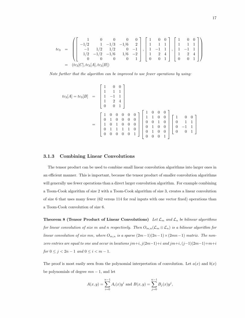
Example 5 A 3× 3 linear convolution given by the Toom-Cook algorithm is:
17
tc3 =
1 0 0 0 0−1/2 1 −1/3 −1/6 2−1 1/2 1/2 0 −11/2 −1/2 −1/6 1/6 −2
0 0 0 0 1
,
1 0 01 1 11 −1 11 2 40 0 1
,
1 0 01 1 11 −1 11 2 40 0 1
= (tc3[C], tc3[A], tc3[B])
Note further that the algorithm can be improved to use fewer operations by using:
tc3[A] = tc3[B] =
1 0 01 1 11 −1 11 2 40 0 1
=
1 0 0 0 0 00 1 0 0 0 01 0 1 0 0 00 1 1 1 1 00 0 0 0 0 1
1 0 0 01 1 0 00 0 1 00 1 0 00 1 0 00 0 0 1
1 0 00 1 10 −1 10 0 1
3.1.3 Combining Linear Convolutions
The tensor product can be used to combine small linear convolution algorithms into larger ones in
an efficient manner. This is important, because the tensor product of smaller convolution algorithms
will generally use fewer operations than a direct larger convolution algorithm. For example combining
a Toom-Cook algorithm of size 2 with a Toom-Cook algorithm of size 3, creates a linear convolution
of size 6 that uses many fewer (62 versus 114 for real inputs with one vector fixed) operations than
a Toom-Cook convolution of size 6.
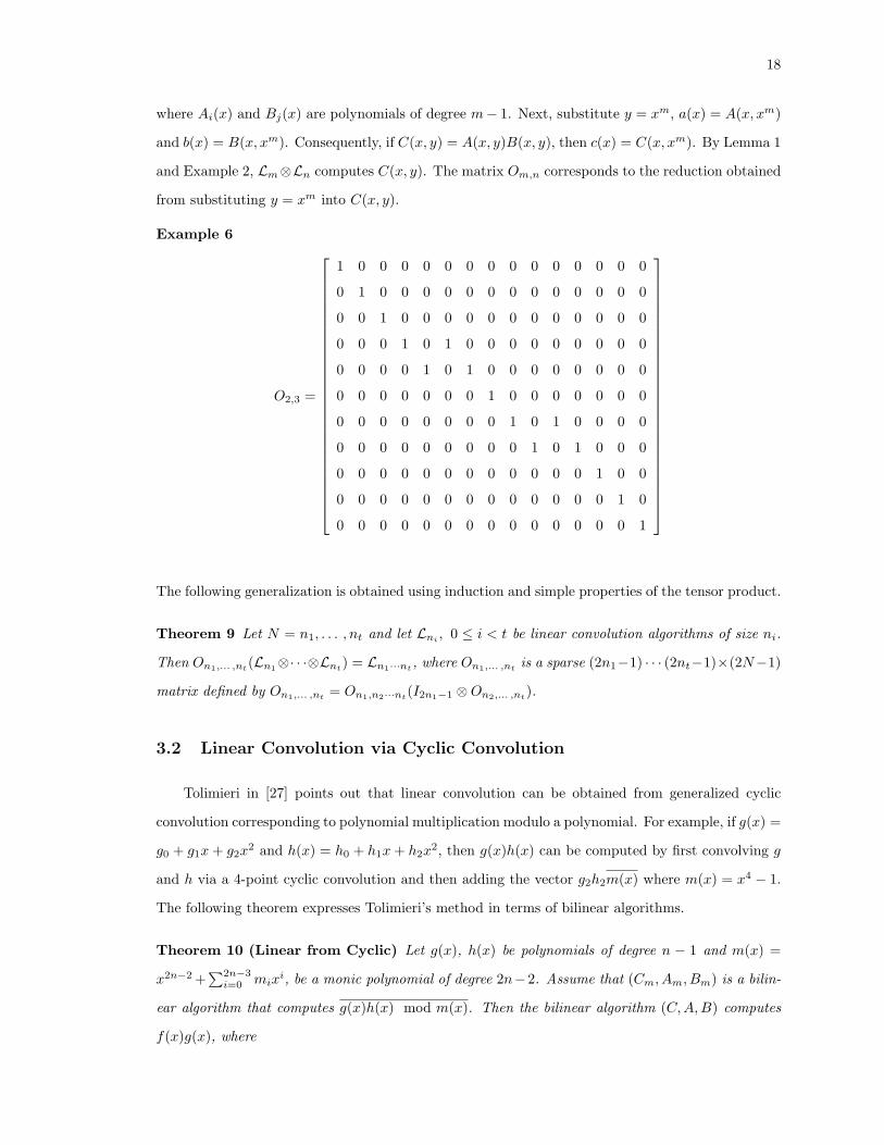
Theorem 8 (Tensor Product of Linear Convolutions) Let Lm and Ln be bilinear algorithms
for linear convolution of size m and n respectively. Then Om,n(Lm⊗Ln) is a bilinear algorithm for
linear convolution of size mn, where Om,n is a sparse (2m−1)(2n−1)×(2mn−1) matrix. The non-
zero entries are equal to one and occur in locations jm+i, j(2m−1)+i and jm+i, (j−1)(2m−1)+m+i
for 0 ≤ j < 2n− 1 and 0 ≤ i < m− 1.
The proof is most easily seen from the polynomial interpretation of convolution. Let a(x) and b(x)
be polynomials of degree mn− 1, and let
A(x, y) =n−1∑
i=0
Ai(x)yi and B(x, y) =n−1∑
j=0
Bj(x)yj ,
18
where Ai(x) and Bj(x) are polynomials of degree m− 1. Next, substitute y = xm, a(x) = A(x, xm)
and b(x) = B(x, xm). Consequently, if C(x, y) = A(x, y)B(x, y), then c(x) = C(x, xm). By Lemma 1
and Example 2, Lm⊗Ln computes C(x, y). The matrix Om,n corresponds to the reduction obtained
from substituting y = xm into C(x, y).
Example 6
O2,3 =
1 0 0 0 0 0 0 0 0 0 0 0 0 0 0
0 1 0 0 0 0 0 0 0 0 0 0 0 0 0
0 0 1 0 0 0 0 0 0 0 0 0 0 0 0
0 0 0 1 0 1 0 0 0 0 0 0 0 0 0
0 0 0 0 1 0 1 0 0 0 0 0 0 0 0
0 0 0 0 0 0 0 1 0 0 0 0 0 0 0
0 0 0 0 0 0 0 0 1 0 1 0 0 0 0
0 0 0 0 0 0 0 0 0 1 0 1 0 0 0
0 0 0 0 0 0 0 0 0 0 0 0 1 0 0
0 0 0 0 0 0 0 0 0 0 0 0 0 1 0
0 0 0 0 0 0 0 0 0 0 0 0 0 0 1
The following generalization is obtained using induction and simple properties of the tensor product.
Theorem 9 Let N = n1, . . . , nt and let Lni , 0 ≤ i < t be linear convolution algorithms of size ni.
Then On1,... ,nt(Ln1⊗· · ·⊗Lnt) = Ln1···nt , where On1,... ,nt is a sparse (2n1−1) · · · (2nt−1)×(2N−1)
matrix defined by On1,... ,nt = On1,n2···nt(I2n1−1 ⊗On2,... ,nt).
3.2 Linear Convolution via Cyclic Convolution
Tolimieri in [27] points out that linear convolution can be obtained from generalized cyclic
convolution corresponding to polynomial multiplication modulo a polynomial. For example, if g(x) =
g0 + g1x + g2x2 and h(x) = h0 + h1x + h2x
2, then g(x)h(x) can be computed by first convolving g
and h via a 4-point cyclic convolution and then adding the vector g2h2m(x) where m(x) = x4 − 1.
The following theorem expresses Tolimieri’s method in terms of bilinear algorithms.
Theorem 10 (Linear from Cyclic) Let g(x), h(x) be polynomials of degree n − 1 and m(x) =
x2n−2 +∑2n−3
i=0 mixi, be a monic polynomial of degree 2n−2. Assume that (Cm, Am, Bm) is a bilin-
ear algorithm that computes g(x)h(x) mod m(x). Then the bilinear algorithm (C,A, B) computes
f(x)g(x), where

19
C =
1 m0
. . ....
1 m2n−3
1
[Cm
1
],
A =[
Am
1
]
1. . .
11
,
B =[
Bm
1
]
1. . .
11
Proof
Let c(x) = g(x)h(x) mod m(x). Therefore, f(x)g(x) = c(x) + q(x)m(x), and since m(x) is monic
and of degree 2n− 2, g(x)h(x) = c(x) + gnhnm(x).
(C, A,B) (g, h) =
1 m0
. . ....
1 m2n−3
1
[Cm (Amg •Bmh)
gnhn
]
= g(x)h(x) mod m(x) + gnhnm(x)
= g(x)h(x).
3.3 Cyclic Convolution
Convolution modulo f(x) refers to polynomial multiplication modulo a third polynomial. Al-
gorithms for convolution modulo f(x) can be obtained from linear convolution algorithms by mul-
tiplying by a matrix, which corresponds to computing the remainder in division by f(x). Let
M(f(x)) denote the reduction matrix defined by M(f(x))A(x) = A(x) mod f(x). The exact form
of M(f(x)) depends on the degree of A(x). If (C, A,B) is a bilinear algorithm for linear convolution,
then (M(f(x))C,A, B) is a bilinear algorithm for convolution modulo f(x).
Example 7 Composing
M(x2 − 1) =
1 0 1
0 1 0
,

20
with the Toom-Cook bilinear algorithm of equation 2.6, the bilinear algorithm
(M(x2 − 1)C2, A2, B2) =
1 0 1
−1 1 −1
,
1 0
1 1
0 1
,
1 0
1 1
0 1
for 2-point cyclic convolution is obtained.
3.3.1 Convolution Theorem
The well-known convolution theorem provides a bilinear algorithm for computing cyclic convolu-
tion.
Theorem 11 (Convolution Theorem)
The bilinear algorithm (DFT−1N , DFTN , DFTN ) computes N -point cyclic convolution.
Proof
Let ωN be a primitive N -th root of unity, then xN−1 =∏N−1
i=0 (x−ωiN ). Since, V[1, ωN , . . . , ωN−1
N ] =
DFTN , the convolution theorem follows from Theorem 3.
When N = RS, xN − 1 =∏S−1
i=0 (xR − ωiS). Applying the Chinese Remainder theorem to
this factorization leads to the following theorem which allows the DFT to be combined with other
convolution algorithms.
Theorem 12 Let N = RS and let Ci, i = 0, . . . , S − 1, be bilinear algorithms to multiply two
polynomials modulo xR − ωiS. Then
(DFT−1S ⊗IR)
(S−1⊕
i=0
Ci
)(DFTS ⊗IR)
is a bilinear algorithm to compute N -point convolution.
Proof
Let f(x) be a polynomial of degree N − 1 and write f(x) =∑S−1
j=0 fj(x)xRj , where deg(fj(x)) < R.
Then f(x) mod xR − ωiS =
∑S−1j=0 fj(x)ωj
S . Therefore, the matrix R = [R0 R1 . . . RS−1]T with
Rif = f(x) mod xR − ωij is equal to DFTS ⊗IR.
Note that multiplication modulo xR − α can easily be transformed into cyclic convolution. Ob-
serve that if βR = α, and h(x) = f(x)g(x) mod xR − α, then
hβ(x) = h(βx) = f(βx)g(βx) (mod (βx)R − α)
= f(βx)g(βx) (mod (βx)R − α)
= f(βx)g(βx) (mod α(xR − 1)).

21
Therefore, h(x) = hβ(x/β).
Applying this observation and the previous theorem leads to the following construction related
to the FFT shown in (2.7).
Theorem 13 Let CR be a bilinear algorithm to compute R-point cyclic convolution, and let FS =
((DFTS ⊗IR), TNR (DFTS ⊗IR), TN
R (DFTS ⊗IR)). Then (IS ⊗ CR)FS computes N -point cyclic con-
volution.
The following example uses Theorem 12 and the matrix exchange theorem to obtain a result that is
similar to Theorem 13 but without the need for Twiddle factors.
Example 8 Let Fn represent a size n FFT, and let α = e2πi/n. Now let Lm = (Cm, Am, Bm)
represent a linear convolution of size m. From Theorem 12 a size mn cyclic convolution is computed
by
(F−1n ⊗ Im)
(n−1⊕
i=0
M(xm − αi)Lm
)(Fn ⊗ Im) (3.1)
Now suppose (C, A, B) is the bilinear algorithm representing the size mn cyclic convolution of (3.1),
then
C = = (F−1n ⊗ Im)
(n−1⊕
i=0
M(xm − αi)Cm
)
A =
(n−1⊕
i=0
Am
)(Fn ⊗ Im)
= (In ⊗Am)(Fn ⊗ Im)
B =
(n−1⊕
i=0
Bm
)(Fn ⊗ Im)
= (In ⊗Bm)(Fn ⊗ Im)
Note that the direct sums for A and B can be changed to tensor products because Am and Bm do
not change with i, (this of course is not true for C).
After applying matrix exchange the following theorem has just been derived and proved.
Theorem 14 (Mixed Convolution Theorem)
Let α = e2πi/n, Fn be a size n FFT, and (Cm, Am, Bm) be a size m linear convolution. Then
J · (Fn ⊗ Im)(In ⊗ATm) ·D · (In ⊗Bm)(Fn ⊗ Im)
22
is a size mn cyclic convolution, where
D =
(n−1⊕
i=0
M(xm − αi)Cm
)T
· (F−1n ⊗ Im) · Jv,
J is the anti-identity matrix, and v is a fixed input vector.
3.3.2 Winograd Convolution Algorithm
Winograd’s algorithm [29] for computing cyclic convolution follows from the Chinese Remainder
Theorem when applied to the irreducible rational factors of the polynomial XN −1. The irreducible
rational factors of xN − 1 are called cyclotomic polynomials.
Definition 7 (Cyclotomic Polynomials)
The cyclotomic polynomials can be defined recursively from the formula
xN − 1 =∏
d|NΦd(x).
Alternatively
ΦN (x) =∏
gcd(j,N)=1
(x− ωjN ),
where ωN is a primitive N -th root of unity. It follows that deg(ΦN (x)) = φ(N), where φ is the
Euler φ function. It is well known [16] that ΦN (x) has integer coefficients and is irreducible over
the rationals.
Applying Theorem 3 to xN − 1 =∏
d|N Φd(x) leads to the following algorithm.
Theorem 15 (Winograd Convolution Algorithm)
Let Cf denote a bilinear algorithm that multiplies elements of C[x]/f(x). Then
R−1
⊕
d|nCΦd(x)
R (3.2)
where R = [Rd1 Rd2 . . . Rdk]T and Rdif = f(x) mod Φdi(x) is a bilinear algorithm for N -point
cyclic convolution.
Using the 2-point cyclic convolution algorithm in Example 7 and the cyclotomic polynomials
Φ1(x) = (x − 1), Φ2(x) = (x + 1), and Φ4(x) = (x2 + 1) the following 4-point cyclic convolution
algorithm is obtained.

23
Example 9
R−14
1
1
1 0 −1
−1 1 −1
,
1
1
1 0
1 1
0 1
R4,
1
1
1 0
1 1
0 1
R4
,
where R4 is the R matrix in Example 1.
The results in the next section provide a more efficient method for computing R4.
3.3.3 CRT-Based Cyclic Convolution Algorithms for Prime Powers
Selesnick and Burrus [22] have shown that when N = pk is a prime power, the Winograd
algorithm has additional structure. This structure follows from the properties
Φp(x) = xp−1 + · · ·+ x + 1
Φpk(x) = Φp(xpk−1).
The composition structure of Φpk(x) provides an efficient way to compute Rpk .
Theorem 16 Let Rpk = [R0, Rp, . . . , Rpk ]t be the pk × pk reduction matrix where Rpif(x) =
f(x) mod Φpi(x) for f(x) of degree pk − 1. Then
Rpk =
1p ⊗Rpk−1
Gp ⊗ Ipk−1
,
where Gn is the (n− 1)× n matrix:
Gn =
1 −1
1 −1. . . −1
1 −1
,
and 1n is the 1× n matrix filled with 1′s. Moreover, Rpk = (Rpk−1 ⊕ I(p−1)pk−1)(Rp ⊗ Ipk−1).
Proof
First observe that if f(x) = f0 + f1x + · · · fm−1xm−1 + xm and A(x) =
∑mi=0 aix
i, then A(x)
mod f(x) =∑m−1
i=0 (ai − fi)xi. Therefore reduction of A(x) modulo f(x) is given by
R =
1 −f0
. . . −f1
1 −fm−1
.

24
When f(x) = 1 + x + · · · + xn−1 the matrix Gn is obtained. Next, observe that if A(x) =∑m
i=0 Ai(x)xni, where deg(Ai) < n, then A(x) mod f(xn) =∑m
i=0(Ai(x)−fiAm(x))xni. Therefore
reduction of A(x) mod f(xn) is given by R⊗In, and reduction modulo Φpk(x) = Φp(xpk−1) is given
by Gp⊗Ipk−1 . Finally, since xpk−1mod Φpk−1 = 1, reduction of A(x) modulo {Φpi(x), i = 0, . . . , k}
is given by 1p ⊗Rpk−1 . These observations prove the first part of the theorem. The factorization in
the second part is obtained using the multiplicative property of the tensor product.
A simple block matrix multiplication provides the following computation of the inverse of Rpk .
Theorem 17
R−1pk = 1/p
(1t
p ⊗R−1pk−1 Vp ⊗ Ipk−1
),
where Vn is the n× (n− 1) matrix
n− 1 −1 −1 . . . −1
−1 n− 1 −1 . . . −1...
. . ....
−1 . . . −1 n− 1 −1
−1 . . . −1 −1 n− 1
−1 . . . −1 −1 −1
Moreover, R−1pk = (R−1
p ⊗ Ipk−1)(R−1pk−1 ⊕ I(p−1)pk−1).
Example 10 A bilinear algorithm for a cyclic convolution of size 27 is (C,A, B), where Ln =
(Ln[C],Ln[A],Ln[B]) is a bilinear algorithm for a linear convolution of size n of any method, and
C = R−133
1M(x2 + x + 1)L2[C]
M(x6 + x3 + 1)L6[C]M(x18 + x9 + 1)L18[C]
,
A =
1L2[A]
L6[A]L18[A]
R33 ,
B =
1L2[B]
L6[B]L18[B]
R33 ,
and
R33 =
1 1 11 0 −10 1 −1
I24
1 1 11 0 −10 1 −1
⊗ I3
I18
1 1 11 0 −10 1 −1
⊗ I9
25
3.3.4 The Agarwal-Cooley and Split-Nesting Algorithms
The Agarwal-Cooley [1] algorithm uses the tensor product to create a larger cyclic convolution
from smaller cyclic convolutions. The Split-Nesting algorithm, due to Nussbaumer [19], follows
directly from Agarwal-Cooley using simple properties of the tensor product.
The Agarwal-Cooley algorithm follows from the fact that when gcd(m,n) = 1, the algebra
F[x]/(xmn − 1) is isomorphic to F[y, z]/(ym − 1, zn − 1), which by Example 2 is isomorphic to
F[y]/(ym − 1) ⊗ F[z]/(zn − 1). The isomorphism is obtained by mapping x to yz which maps xi
to y(i mod m)z(i mod n). Using the reordering required by this mapping and Lemma 1 leads to the
following theorem which shows how to build an mn-point cyclic convolution algorithm from the
tensor product of m-point and n-point cyclic convolution algorithms.
Theorem 18 (Agarwal-Cooley Algorithm)
Assume gcd(m,n) = 1 and let Cm = (Cm, Am, Bm) and Cn = (Cn, An, Bn) be bilinear algorithms
for cyclic convolution of size m and n. Let Q−1m,n be the permutation that maps i to (i mod m)n+(i
mod n). Then Q−1m,n(Cm ⊗ Cn)Qm,n computes a cyclic convolution of size mn.
The permutation Qm,n is defined by the mapping in + j 7→ iem + jen mod mn, 0 ≤ i < m,
0 ≤ j < n, where em ≡ 1 mod m, em ≡ 0 mod n, en ≡ 0 mod m, en ≡ 1 mod n, are the
idempotents defining the Chinese remainder theorem mapping for the integers m and n.
Let R−1m
(⊕k1i=0 Cmi
)Rm and R−1
n
(⊕k2i=0 Cni
)Rn be bilinear algorithms to compute m, and n-
point Winograd cyclic convolutions. Then combining Agarwal-Cooley with the Winograd algorithm
yields the bilinear algorithm
Q−1m,n
(R−1
m
(k1⊕
i=0
Cmi
)Rm
)⊗
R−1
n
k2⊕
j=0
Cnj
Rn
Qm,n (3.3)
for computing an mn-point cyclic convolution, (provided gcd(m,n) = 1). Using the multiplicative
property of the tensor product, this is equal to
Q−1m,n(R−1
m ⊗R−1n )
(k1⊕
i=0
Cmi
)⊗
k2⊕
j=0
Cnj
(Rm ⊗Rn)Qm,n. (3.4)
Rearranging this equation into a double sum of tensor products leads to the “Split-Nesting
Algorithm” which was first derived by Nussbaumer [19], who observed that it requires fewer additions
then equation 3.3. The following theorem describes this transformation.

26
Theorem 19 (Split Nesting) Let C =⊕s−1
i=0 Ci and D =⊕t−1
j=0Dj. Then
C ⊗ D = P−1
s−1⊕
i=0
t−1⊕
j=0
Ci ⊗Dj
P,
where P is a permutation.
Proof
Using the first part of Theorem 6,
C ⊗ D =s−1⊕
i=0
Ci ⊗t−1⊕
j=0
Dj =s−1⊕
i=0
Ci ⊗
t−1⊕
j=0
Dj
.
Using the second part of Theorem 6, the previous equation is equal to
s−1⊕
i=0
P−1i
t−1⊕
j=0
Ci ⊗Dj
Pi, which is equal to P−1
s−1⊕
i=0
t−1⊕
j=0
Ci ⊗Dj
P,
where P =⊕s−1
i=0 Pi.
Example 11 Let C4 = R−14 (1⊕ 1⊕ C2)R4 and C27 = R−1
27 (1⊕D2 ⊕D6 ⊕D18)R27, where
C2 = M(x2+1)L2, D2 = M(x2+x+1)L2, D6 = M(x6+x3+1)L6, D18 = M(x18+x9+1)L18, are the
algorithms for cyclic convolution on 4 and 27 points given in Examples 9 and 10. By Agarwal-Cooley,
Q−14,27(R
−14 (1⊕ 1⊕ C2)R4)⊗ (R−1
27 (1⊕D2 ⊕D6 ⊕D18)R27)Q4,27
is an algorithm for cyclic convolution on 108 points. The split nesting theorem transforms this
algorithm into
(Q−14,27(R
−14 ⊗R−1
27 )P−1
(1⊕D2⊕D6⊕D18)⊕(1⊕D2⊕D6⊕D18)⊕(C2⊕C2⊗D2⊕C2⊗D6⊕C2⊗D18))
P (R4 ⊗R27)Q4,27
where P = I27 ⊕ I27 ⊕ P3 and P3 = (I2 ⊕ L42 ⊕ L12
2 ⊕ L362 )L54
27.
3.3.5 The Improved Split-Nesting Algorithm
The split-nesting algorithm combined with the prime power algorithm provides a method for
computing any size cyclic convolution. Since the prime power algorithm consists of direct sums of
linear convolutions combined with various reductions, and the split-nesting algorithm commutes the
direct sums and tensor products, all cyclic convolutions computed via split-nesting become direct
sums of reduced tensor products of linear convolutions. It may not be immediately clear as yet, but

27
in fact, any of the linear convolutions and tensor products of linear convolutions can be replaced by
other linear convolutions or tensor products of linear convolutions. This is the main idea behind the
improved split-nesting algorithm. Simply stated, the improved split-nesting algorithm replaces any
linear convolution or tensor product of linear convolutions, with optimal substitutes. Here optimal
may mean fastest run-time, fewest operations, etc.
Example 12 To make this idea more clear, consider example 11 again. One of the components of
this algorithm is C2 ⊗ D18, where C2 = M(x2 + 1)L2 and D18 = M(x18 + x9 + 1)L18, so that this
component is really (M(x2 +1)⊗M(x18 +x9 +1))(L2⊗L18) or more generally a reduction composed
with a tensor product of two linear convolutions (e.g. M(L2 ⊗ L18)).
It will be shown in chapter 6 that the optimal L2 is the Toom-Cook linear algorithm tc2 that
requires 6 operations, and that the optimal L18 is O3,2,3sb3⊗ tc2⊗ tc3, that is obtained by combining
the standard algorithm of size 3 with Toom-Cook’s of size 2 and 3. It will be shown in chapter 6 that
this algorithm requires 366 operations.
Next note that L2 ⊗ L18 is related to L36 since the latter is just O2,18(L2 ⊗ L18). Because of
matrix exchange, the O matrix has no cost, so that the number of operations required for L2 ⊗L18,
is the same as that of L36.
Table 3.1 below, shows a table of size 36 convolutions built using the methodology discussed in
chapter 6. If the optimal L2 and L18 are chosen, the algorithm for L2⊗L18 would cost the same as
Lin36i, or 1272 operations. However the improved split-nesting algorithm would substitute Lin36d,
which could be made equivalent to L2 ⊗ L18 via the commutation theorem. That is,
L2 ⊗ L18 = tc2 ⊗O3,2,3(sb3 ⊗ tc2 ⊗ tc3)= (I3 ⊗O3,2,3)(tc2 ⊗ sb3 ⊗ tc2 ⊗ tc3) (3.5)= (I3 ⊗O3,2,3)(L15
3 (sb3 ⊗ tc2)L63 ⊗ tc2 ⊗ tc3) (3.6)
Note that (3.5) is related to Lin36i requiring 1272 operations, and that (3.6) is related to Lin36d
requiring only 1092 operations. Thus the cost of the size 108 cyclic convolution can be reduced by at
least 180 operations via the improved split-nesting algorithm.
In Chapter 4 an infrastructure is discussed that automates the implementation of the algorithms
discussed in this chapter.

28
Table 3.1: Operation Counts for Linear Convolution
B B At At Diag TotalMethod Adds Muls Adds Muls Muls OpsLin36a = O3,3,2,2(sb3 ⊗ sb3 ⊗ tc2 ⊗ tc2) 45 0 738 0 729 1512Lin36b = O3,2,3,2(sb3 ⊗ tc2 ⊗ sb3 ⊗ tc2) 99 0 792 0 729 1620Lin36c = O3,2,2,3(sb3 ⊗ tc2 ⊗ tc2 ⊗ sb3) 135 0 828 0 729 1692Lin36d = O3,2,2,3(sb3 ⊗ tc2 ⊗ tc2 ⊗ tc3) 159 0 528 0 405 1092Lin36e = O3,2,3,2(sb3 ⊗ tc2 ⊗ tc3 ⊗ tc2) 189 0 558 0 405 1152Lin36f = O3,3,2,2(sb3 ⊗ tc3 ⊗ tc2 ⊗ tc2) 234 0 603 0 405 1242Lin36g = O2,3,3,2(tc2 ⊗ sb3 ⊗ sb3 ⊗ tc2) 261 0 954 0 729 1944Lin36h = O2,3,2,3(tc2 ⊗ sb3 ⊗ tc2 ⊗ sb3) 297 0 990 0 729 2016Lin36i = O2,3,2,3(tc2 ⊗ sb3 ⊗ tc2 ⊗ tc3) 249 0 618 0 405 1272Lin36j = O2,3,3,2(tc2 ⊗ sb3 ⊗ tc3 ⊗ tc2) 279 0 648 0 405 1332Lin36k = O2,2,3,3(tc2 ⊗ tc2 ⊗ sb3 ⊗ sb3) 405 0 1098 0 729 2232Lin36l = O2,2,3,3(tc2 ⊗ tc2 ⊗ sb3 ⊗ tc3) 309 0 678 0 405 1392Lin36m = O2,2,3,3(tc2 ⊗ tc2 ⊗ tc3 ⊗ sb3) 477 0 846 0 405 1728Lin36n = O2,2,3,3(tc2 ⊗ tc2 ⊗ tc3 ⊗ tc3) 349 0 538 0 225 1112Lin36o = O2,3,3,2(tc2 ⊗ tc3 ⊗ sb3 ⊗ tc2) 531 0 900 0 405 1836Lin36p = O2,3,2,3(tc2 ⊗ tc3 ⊗ tc2 ⊗ sb3) 567 0 936 0 405 1908Lin36q = O2,3,2,3(tc2 ⊗ tc3 ⊗ tc2 ⊗ tc3) 399 0 588 0 225 1212Lin36r = O2,3,3,2(tc2 ⊗ tc3 ⊗ tc3 ⊗ tc2) 429 0 618 0 225 1272Lin36s = O3,3,2,2(tc3 ⊗ sb3 ⊗ tc2 ⊗ tc2) 612 0 981 0 405 1998Lin36t = O3,2,3,2(tc3 ⊗ tc2 ⊗ sb3 ⊗ tc2) 666 0 1035 0 405 2106Lin36u = O3,2,2,3(tc3 ⊗ tc2 ⊗ tc2 ⊗ sb3) 702 0 1071 0 405 2178Lin36v = O3,2,2,3(tc3 ⊗ tc2 ⊗ tc2 ⊗ tc3) 474 0 663 0 225 1362Lin36w = O3,2,3,2(tc3 ⊗ tc2 ⊗ tc3 ⊗ tc2) 504 0 693 0 225 1422Lin36x = O3,3,2,2(tc3 ⊗ tc3 ⊗ tc2 ⊗ tc2) 549 0 738 0 225 1512
29
Chapter 4: Implementation of Convolution Algorithms
In this chapter, a Maple package for implementing the algorithms discussed in previous chapters
is described. The implementation is based on a programming language called SPL and a Maple
infrastructure that aids in the creation and manipulation of SPL code. The latest version of the
SPL Compiler can be obtained at http://www.ece.cmu.edu/∼spiral/ and the latest version of the
Maple package can be obtained at http://www.cs.drexel.edu/techreports/2000/abstract0002.html.
4.1 Overview of SPL and the SPL Maple Package
Having codified known convolution techniques into a common framework of bilinear algorithms
built from parameterized matrices and algebraic operators, Maple’s symbolic and algebraic compu-
tation facilities are used to derive and manipulate these algorithms. The infrastructure provided by
the package allows for the generation, manipulation, testing, and combining of various convolution
algorithms within an interactive environment. The algorithms generated by the package can be ex-
ported to a domain-specific language called SPL (Signal Processing Language) and then translated
into efficient C or FORTRAN code by the SPL compiler. By combining the strengths of Maple and
the SPL compiler the benefits of existing algebraic computation tools are realized without the need
to embed high-performance compiler technology in a computer algebra system.
The resulting environment allows one to systematically apply the algebraic theory developed over
the years to produce correct and efficient programs. Numerous algorithmic choices can be tried,
allowing the user to rapidly test various optimizations to find the best combination of algorithms
for a particular size convolution on a particular computer. Furthermore, automatic code generation
and algebraic verification provides the ability to construct non-trivial examples with confidence that
the resulting code is correct.
4.1.1 SPL Language
This section briefly outlines the SPL language. Further details are available in [31], where, in
addition, an explanation of how SPL programs are translated to programs is provided.
SPL provides a convenient way of expressing matrix factorizations, and the SPL compiler trans-
lates matrix factorizations into efficient programs for applying the matrix expression to an input
vector. SPL programs consist of the following: 1) SPL formulas, which are symbolic expressions

30
used to represent matrix factorizations, 2) constant expressions for entries appearing in formulas;
3) “define statements” for assigning names to subexpressions; and 4) compiler directives, which are
used to change the behavior of the SPL compiler in some way (e.g. to turn loop unrolling on or off).
SPL formulas are built from general matrix constructions, parameterized symbols denoting families
of special matrices, and matrix operations such as matrix composition, direct sum, and the tensor
product. The elements of a matrix can be real or complex numbers. In SPL, these numbers can
be specified as scalar constant expressions, which may contain function invocations and symbolic
constants like pi. For example, 12, 1.23, 5*pi, sqrt(5), and (cos(2*pi/3.0),sin(2*pi/3)) are
valid scalar SPL expressions. All constant scalar expressions are evaluated at compile-time. SPL
uses a prefix notation similar to lisp to represent formulas. SPL code is compiled into C or FOR-
TRAN by invoking the SPL compiler and entering the lisp like SPL formulas interactively, or by
sending a text file of the SPL formulas to the SPL compiler.
General matrix constructions. Examples include the following.• (matrix (a11 ... a1n)...(am1 ... amn)) - the m×n matrix [aij ]0≤i<m, 0≤j<n.• (sparse (i1 j1 ai1j1) . . . (it jt aitjt)) - the m × n matrix where m = max(i1, . . . , it),
n = max(j1, . . . , jt) and the non-zero entries are aikjkfor k = 1, . . . , t.
• (diagonal (a1 ... an)) - the n× n diagonal matrix diag(a1, . . . , an).• (permutation (σ1 ... σn)) - the n× n permutation matrix: i 7→ σi, for i = 1, . . . , n.
Parameterized Symbols. Examples include the following.• (I n) - the n× n identity matrix In.• (F n) - the n× n DFT matrix Fn.• (L mn n) - the mn×mn stride permutation matrix Lmn
n .• (T mn n) - the mn×mn twiddle matrix Tmn
n .Matrix operations. Examples include the following.
• (compose A1 ... At) - the matrix product A1 · · ·At.• (direct-sum A1 ... At) - the direct sum A1 ⊕ · · · ⊕At.• (tensor A1 ... At) - the tensor product A1 ⊗ · · · ⊗At.• (conjugate A P) - the matrix conjugation AP = P−1 ·A · P , where P is a permutation.
It is possible to define new general matrix constructions, parameterized symbols, and matrix
operations using a template mechanism. To illustrate how this is done, an example showing how to
add the stack operator to SPL is given. Let A and B be m × n and p × n matrices respectively,
then (stackAB) is the (m + p)× n matrix A
B
.
Given a program to apply A to a vector and a program to apply B to a vector, a program to apply
(stack A B) to a vector is obtained by applying A to the input and storing the result in the first
m elements of the output and applying B to the input and storing the result in the remaining p
elements of the output. The following SPL template enables the SPL compiler to construct code
31
for (stack A B) using this approach. (This example is given to illustrate that a process exists for
adding new functionality to SPL; the reader need not be concerned with the specific syntax.)
(template (stack any any)[$p1.nx == $p2.nx](
$y(0:1:$p1.ny_1) = call $p1( $x(0:1:$p1.nx_1) )$y($p1.ny:1:$p0.ny_1) = call $p2( $x(0:1:$p1.nx_1) )
))
The first part of the template is the pattern (stack any any) which matches (stack A B) where
A and B match any SPL formulas. The code for A and B is accessed through the call statements,
where A is referenced as $p1 and B is referenced as $p2. The field nx refers to the input dimension
and ny refers to the output dimension ( 1 subtracts one).
4.1.2 SPL Maple Package
Programming directly in SPL is a cumbersome process, creating a need to provide an interactive
version of SPL in Maple (or some other interactive scripting environment). In this environment, it
is much easier to add new features and to extend the language, and it is possible to write simple
scripts, using Maple’s algebraic computation engine to generate SPL code [18]. In particular, SPL
was extended to include bilinear computations in addition to linear computations. Also all of the
parameterized matrices and bilinear algorithms discussed in chapter 3 were added, and Maple’s
polynomial algebra capabilities were exploited to generate SPL objects obtained from the Chinese
remainder theorem.
This implementation centers around the concept of an SPL object, which corresponds to a multi-
linear computation. SPL objects have a name, a type, (the default type is complex), and fields that
indicate the number of inputs as well as the input and output dimensions. In addition, there may
be a list of parameters which may be set to Maple expressions such as an integer, list, or polynomial
or other SPL objects. Since parameters include both primitive data types and SPL objects, an SPL
object can be used to represent general matrix constructions, parameterized matrices, or operators.
There are methods to construct an SPL object, evaluate an SPL object to a matrix or a triple of
matrices in the case of bilinear algorithms, apply an SPL object, count the number of arithmetic
operations used by an SPL object, and export an SPL object. Once exported an SPL object can be
compiled by the SPL compiler.
SPL objects can be bound or unbound. An unbound object is a named, parameterized, multi-
linear map which does not have a specified method of computation (i.e. it does not have an apply
method). Alternatively, an SPL object may have an apply method, but be considered unbound

32
because one or more of its parameters are unbound. Unbound objects can be bound by using a
provided bind function. The bind function allows SPL objects to be defined in terms of other SPL
objects. Parameterized matrices and operators may be defined using other parameterized matrices
and operators. Since the SPL objects defining an SPL object may themselves be unbound, bind
may need to be applied recursively. It is possible to specify the number of levels that bind is to be
applied.
Using unbound symbols has several advantages: 1) the size of an SPL expression can be sig-
nificantly shorter when symbols are not always expanded, 2) it is easier to see the structure in a
complicated formula if sub-formulas are named, 3) parameterized matrices and operators not avail-
able to the SPL compiler can be used provided a bind function is available that defines them using
formulas supported by the compiler, and 4) an SPL expression can be constructed whose components
are unspecified and therefore, alternative computation methods can be used when applying an SPL
object. The last point can be used to apply the optimization techniques presented in Section 3.3.5
(e.g. the improved split-nesting algorithm).
4.2 Implementation Details of Core SPL Package
SPL is a language for creating fast algorithms for linear computations based on combinations of
the symbols and operators discussed in section 4.1.1. The Core SPL Maple package is designed to
ease the use of SPL. Specifically, the interactive environment of the Core SPL package can be used
to apply vectors to both linear and bilinear algorithms, to easily create new symbols or operators,
to view linear algorithms and bilinear algorithms as matrices, to count the number of operations
required to apply an arbitrary vector or vectors to linear and bilinear algorithms, and ultimately, to
generate SPL code that can then be compiled by the SPL compiler.
4.2.1 Core SPL Commands
The basic input and output of the package is called an ‘SPLObject.’ An SPLObject is made up
of sequences of SPL matrices and operators. There are five basic SPL commands that act on SPL
objects:
1. SPLEval(T:SPL object) Evaluates an SPL object into a corresponding matrix.
2. SPLApply(T:SPL object) Applies a vector to the SPL object to obtain an output vector.
3. SPLCountOps(T:SPL object,[adds,muls,assigs]) Counts the number of operations requiredto apply a vector to an SPL object. If adds, muls, and assigs are included, the counts arereturned in these variables, otherwise the counts are printed to the screen.

33
4. SPLBind(T:SPL object,[bindLevel:posint]) Binds a named SPL object to an actual SPLobject. If bindLevel is ∞ or omitted, it completely binds the object, otherwise it binds theobject bindLevel steps.
5. SPLPrint(T:SPL object,[bindLevel:posint],[fDesc:file descriptor]) Shows the SPLobject as a sequence of SPL commands. The default behavior is to print the sequence to thescreen, unless a file descriptor is provided as the third argument. A bind-level can be passedin as an optional second argument. If a bind level is provided, the command is equivalent toSPLPrint(SPLBind(T,bindLevel)).
An SPL object can also represent a bilinear algorithm, which is simply a triple of matrices. In
the case of bilinear algorithms SPLEval evaluates the bilinear SPL object into a triple of matrices,
SPLApply applies a pair of vectors to the bilinear SPL object to obtain an output vector, or applies
a single vector to the bilinear object to obtain a linear algorithm.
4.2.2 Core SPL Objects
The five commands discussed above allow a user to act on SPL objects representing either linear
or bilinear algorithms. All that is needed now is a mechanism to create SPL objects. In this section
the kinds of SPL objects that can be created within the core package are discussed. In SPL, there
are two fundamental types of SPL objects: parameterized matrices and operators. For example,
(I n) is a parameterized matrix that takes a size n and returns an Identity matrix of the specified
size, while (compose ...) is an operator that acts on two or more SPL objects. Within the Core
package there are parameterized matrices and operators as well, but the package was designed so
that either type of object can be represented with the same data structure. This allows for a very
simple implementation of the five basic commands discussed above.
The list of all available parameterized matrices and operators provided within the Core Maple
package can be found in tables 4.1 and 4.2 below.
SPLBilinear is an unusual operator that warrants more discussion. This operator operates on
a set of 3 SPL objects to represent a bilinear algorithm. Note that all of the other operators can
operate on bilinear algorithms as well as linear algorithms (matrices), and that if the inputs are
linear algorithms than the output will be linear algorithms, and similarly for bilinear algorithms.
Once again, a bilinear algorithm is simply a triple of linear algorithms, and the only way to convert
a bilinear algorithm to a linear algorithm is to apply a single vector to either of the two inputs.

34
Table 4.1: Core Maple Parameterized Matrices
Bound SymbolsSPLDiagonal(d1,...,dn) Diagonal matrix of entries d1, . . . , dn
SPLFourier(n,omega) n× n Fourier Matrixwith optional argument omega
SPLIdentity(r,c) r × c (c optional) identity matrixSPLAntiIdentity(n) n× n Anti-identity matrixSPLMatrix([[a11,a12,...],
[a21,a22,...],...]) Entry specified matrixSPLPermutation([p1,...,pn]) Permutation matrixSPLPermutationInv([p1,...,pn]) Inverse or reverse permutation MatrixSPLSparse([[i,j,aij],...]) Sparse matrix with non-zero entries specifiedSPLStride(mn,n) Stride permutationSPLTwiddle(n,[omega]) Twiddle matrixSPLZeroMatrix(r,c) r × c zero matrixUnbound SymbolsSPLOnes(m,n) m× n matrix with all entries equal to 1.
Implementation of Bound Objects in the Core Package
The package was built so that new symbols and operators could be added with relative ease,
and so that new symbols would not require changes to existing symbols and operators. In order
to gain that flexibility, all new objects must provide a constructor that returns an SPL object, and
each object must supply its own Apply, Eval, Print, and Count functions. In this way, nothing is
assumed about SPL objects by the package, and thus there are no built-in limitations.
As mentioned above, in the SPL language, there are two types of objects: symbols and operators.
However, removing this distinction simplifies the implementation and provides a more uniform view;
in later sections it will be shown that the implementation of convolution algorithms is equivalent
to writing down SPL objects as one might write down the formulas for each convolution algorithm
found in Chapter 3. It is therefore useful to think generically of SPL objects rather than symbols
and operators. in the Maple package all SPL objects, whether operators or symbols are treated the
same and implemented in the same manner.
Every SPL object must have the following fields defined within its constructor:
1. apply - This is a pointer to an apply function for the object. The apply function allows theuser to apply a vector to an object.
2. bind - This is a pointer to a bind function. For bound objects this is set to NULL, forunbound objects this points to a function that will rewrite the unbound object into a sequenceof bound objects.
3. countOps - This is a pointer to a function that counts the number of operations required toapply a vector to the object.

35
4. eval - This is a pointer to an evaluation function, that will display the object as a matrix, ortriple of matrices if the object is bilinear.
5. inv - This is a pointer of a function that will create the object’s inverse when it exists. (Notethat inverse and transpose are not implemented in the SPL compiler.)
6. print - This is a pointer to a function that prints the object into SPL code.
7. vecInputs - This specifies whether the object accepts 1 vector (linear), 2 vectors, (bilinear)etc. Although only linear and bilinear objects are currently supported, there is no reason whythe package couldn’t be slightly modified to support trilinear and multilinear objects.
8. trans - This is a pointer to a function that can create an object’s transpose.
9. name - A name for the object (e.g. compose, matrix, sparse, etc.). This is the name printedby the print function, and corresponds to a name recognized by the SPL compiler in the caseof bound objects.
10. rowdim - Row dimension of the object.
11. coldim - Column dimension of the object.
12. parameters - Parameters of the object. For example for Identity, the parameters are therow and column dimension, while for matrix the parameter is a list of rows.
13. numParameters - The number of parameters. This is useful for cases such as compose, wherethere can be a variable number of input parameters.
14. bound - Is the object bound? As discussed below, the existence of a bind function is notsufficient to determine whether an object is bound. (This parameter and the next parametercould be avoided by using an isBound function, but instead these items are stored to improvespeed.)
15. parametersBound - Are an objects’ parameters bound? For example an object might be acomposition of several unbound SPL objects.
In short, an SPL object is simply a Maple table (a Maple table is basically an associative array,
see [18]) with these 15 fields defined as well as the corresponding eval, apply, and other functions
provided. It is useful to conceptually think of an SPL object as a table with these 15 fields, however to
save space the first eight fields in the list above (which are static) are stored in a separate associative
array indexed by the object’s name, so that only the next seven fields actually have to be stored in
the object’s table. This implementation can lead to substantial savings in the size of the table used
to store an SPL object. For example, for large convolution algorithms it is not uncommon to have
more than 100 identity matrices involved in the computation. By storing the eight static fields, more
than 800 objects are removed from the SPL object table. (Actually the savings would be larger,
because the same system is used for all symbols and operators).
To make the discussion clearer, consider the implementation of SPLIdentity. The complete code
for SPLIdentity is shown below. The entries to the global table symTabl are assigned when the
package is loaded. Whenever an identity object is needed, the user calls the constructor SPLIdentity

36
Table 4.2: Core Maple Operators
Bound OperatorsSPLAdd(m1,...,mn) Add SPL objectsSPLCompose(m1,...,mn) Compose SPL objectsSPLConjugate(m,Pinv,P) Equivalent to SPLCompose(Pinv,m,P)SPLDirectSum(m1,...,mn) Direct sum of SPL objectsSPLInverse(m) Inverse of SPL objectSPLTensor(m1,...,mn) Tensor product of SPL objectsSPLTranspose(m) Transpose of SPL objectUnbound OperatorsSPLBilinear(c,a,b) Create a bilinear object from 3 SPL objectsSPLAugmentMatrix(m1,...,mn) Augment matricesSPLStackMatrix(m1,...,mn) Stack matricesSPLConvertPerm(P) Converts an SPL expression P, that represents a sequence of
operations on permutations, into a single permutation. (e.g.SPLTensor(p1, p2) can be converted to a single permutation)
SPLTensorI(m1,...,mn) (m1 ⊗ I)(I ⊗m2 ⊗ I) . . . (I ⊗mn)SPLCommuteTensorI(m1,m2) Commutation theorem for linear
and bilinear algorithms
with the desired dimensions as parameters. Since the constructor does little more than check for
errors and fill in the seven variable fields discussed above, the constructor for identity is very similar
to the constructors for most other SPL objects. All of the functionality of the SPL objects are
defined in the functions pointed to within the symbol table as is shown here.
###################################################################### Identity Matrix# Inputs:# n : positive integer.# Notation: (I m n) or (I n)# Properties: permutation, symmetric.# Definition (I n) i -> i.#####################################################################
symTabl["I"][apply] := applyIdentity;symTabl["I"][bind] := NULL;symTabl["I"][countOps] := countOpsIdentity;symTabl["I"][eval] := evalIdentity;symTabl["I"][inv] := invIdentity;symTabl["I"][print] := defaultSymPrint;symTabl["I"][vecInputs] := 1;symTabl["I"][trans] := transIdentity;
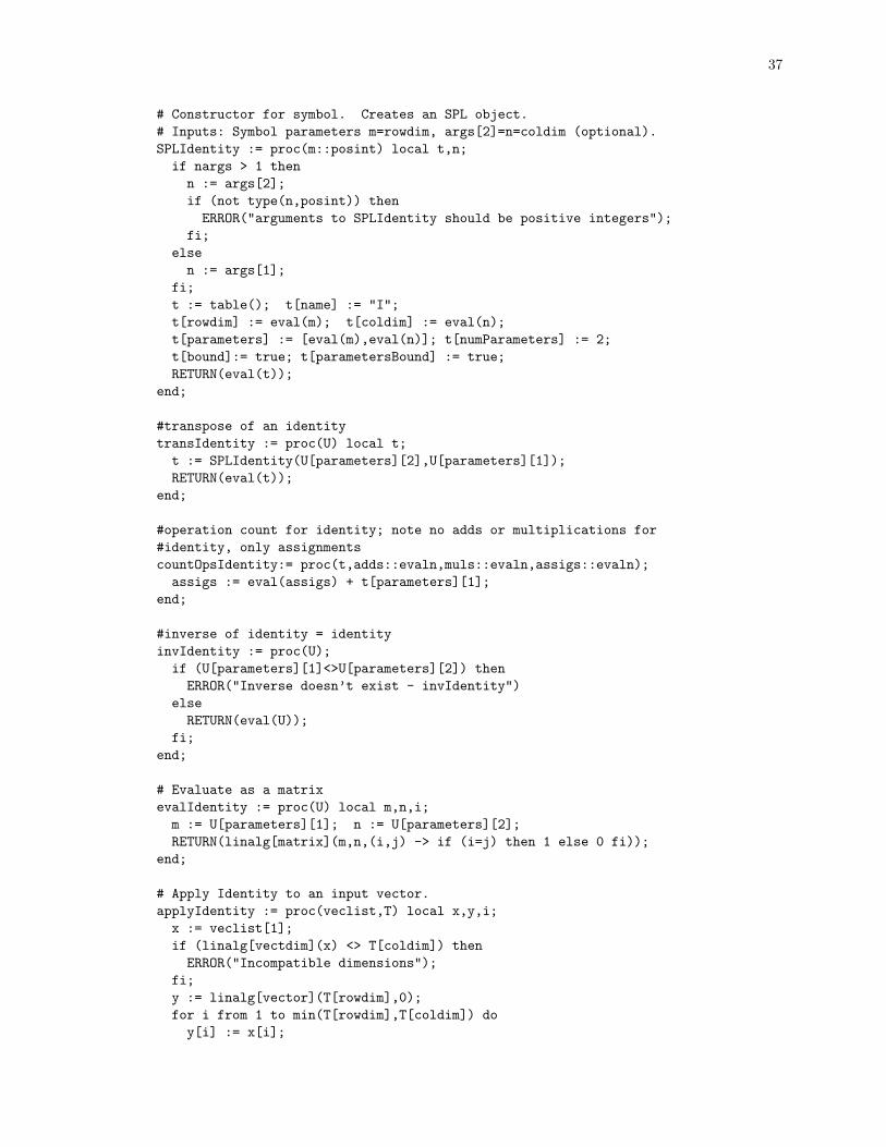
37
# Constructor for symbol. Creates an SPL object.# Inputs: Symbol parameters m=rowdim, args[2]=n=coldim (optional).SPLIdentity := proc(m::posint) local t,n;
if nargs > 1 thenn := args[2];if (not type(n,posint)) thenERROR("arguments to SPLIdentity should be positive integers");
fi;else
n := args[1];fi;t := table(); t[name] := "I";t[rowdim] := eval(m); t[coldim] := eval(n);t[parameters] := [eval(m),eval(n)]; t[numParameters] := 2;t[bound]:= true; t[parametersBound] := true;RETURN(eval(t));
end;
#transpose of an identitytransIdentity := proc(U) local t;
t := SPLIdentity(U[parameters][2],U[parameters][1]);RETURN(eval(t));
end;
#operation count for identity; note no adds or multiplications for#identity, only assignmentscountOpsIdentity:= proc(t,adds::evaln,muls::evaln,assigs::evaln);
assigs := eval(assigs) + t[parameters][1];end;
#inverse of identity = identityinvIdentity := proc(U);
if (U[parameters][1]<>U[parameters][2]) thenERROR("Inverse doesn’t exist - invIdentity")
elseRETURN(eval(U));
fi;end;
# Evaluate as a matrixevalIdentity := proc(U) local m,n,i;
m := U[parameters][1]; n := U[parameters][2];RETURN(linalg[matrix](m,n,(i,j) -> if (i=j) then 1 else 0 fi));
end;
# Apply Identity to an input vector.applyIdentity := proc(veclist,T) local x,y,i;
x := veclist[1];if (linalg[vectdim](x) <> T[coldim]) then
ERROR("Incompatible dimensions");fi;y := linalg[vector](T[rowdim],0);for i from 1 to min(T[rowdim],T[coldim]) do
y[i] := x[i];
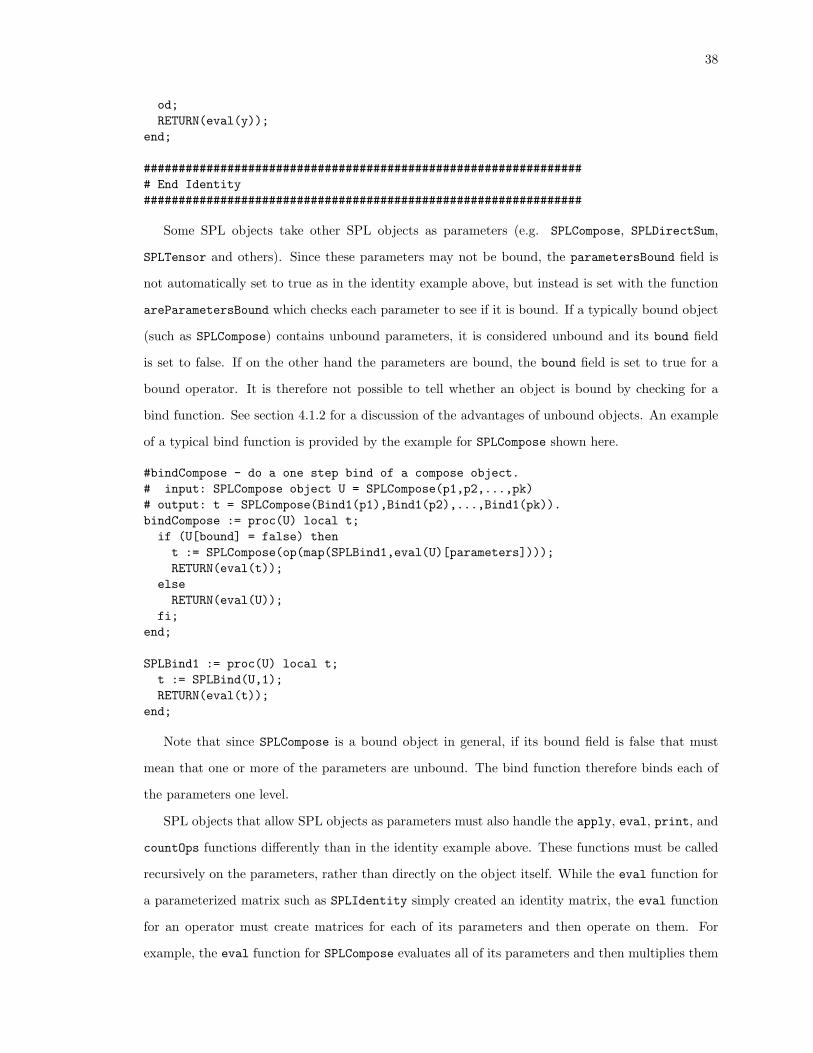
38
od;RETURN(eval(y));
end;
################################################################ End Identity###############################################################
Some SPL objects take other SPL objects as parameters (e.g. SPLCompose, SPLDirectSum,
SPLTensor and others). Since these parameters may not be bound, the parametersBound field is
not automatically set to true as in the identity example above, but instead is set with the function
areParametersBound which checks each parameter to see if it is bound. If a typically bound object
(such as SPLCompose) contains unbound parameters, it is considered unbound and its bound field
is set to false. If on the other hand the parameters are bound, the bound field is set to true for a
bound operator. It is therefore not possible to tell whether an object is bound by checking for a
bind function. See section 4.1.2 for a discussion of the advantages of unbound objects. An example
of a typical bind function is provided by the example for SPLCompose shown here.
#bindCompose - do a one step bind of a compose object.# input: SPLCompose object U = SPLCompose(p1,p2,...,pk)# output: t = SPLCompose(Bind1(p1),Bind1(p2),...,Bind1(pk)).bindCompose := proc(U) local t;
if (U[bound] = false) thent := SPLCompose(op(map(SPLBind1,eval(U)[parameters])));RETURN(eval(t));
elseRETURN(eval(U));
fi;end;
SPLBind1 := proc(U) local t;t := SPLBind(U,1);RETURN(eval(t));
end;
Note that since SPLCompose is a bound object in general, if its bound field is false that must
mean that one or more of the parameters are unbound. The bind function therefore binds each of
the parameters one level.
SPL objects that allow SPL objects as parameters must also handle the apply, eval, print, and
countOps functions differently than in the identity example above. These functions must be called
recursively on the parameters, rather than directly on the object itself. While the eval function for
a parameterized matrix such as SPLIdentity simply created an identity matrix, the eval function
for an operator must create matrices for each of its parameters and then operate on them. For
example, the eval function for SPLCompose evaluates all of its parameters and then multiplies them
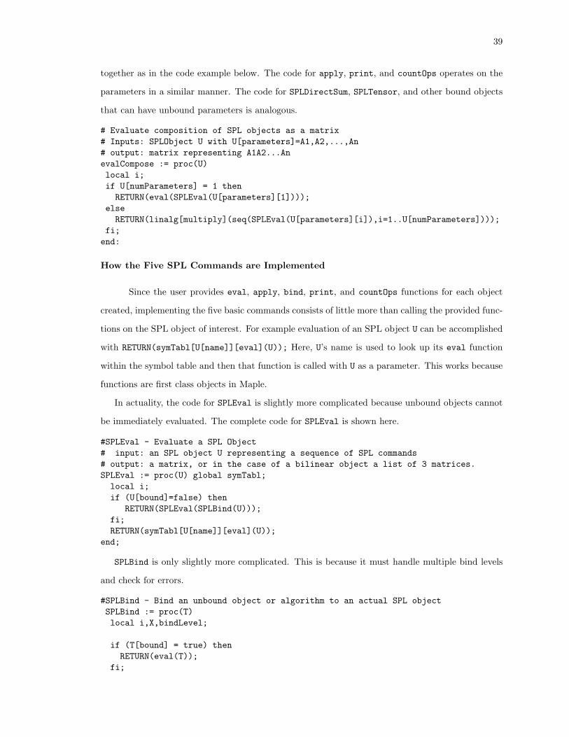
39
together as in the code example below. The code for apply, print, and countOps operates on the
parameters in a similar manner. The code for SPLDirectSum, SPLTensor, and other bound objects
that can have unbound parameters is analogous.
# Evaluate composition of SPL objects as a matrix# Inputs: SPLObject U with U[parameters]=A1,A2,...,An# output: matrix representing A1A2...AnevalCompose := proc(U)local i;if U[numParameters] = 1 then
RETURN(eval(SPLEval(U[parameters][1])));else
RETURN(linalg[multiply](seq(SPLEval(U[parameters][i]),i=1..U[numParameters])));fi;
end:
How the Five SPL Commands are Implemented
Since the user provides eval, apply, bind, print, and countOps functions for each object
created, implementing the five basic commands consists of little more than calling the provided func-
tions on the SPL object of interest. For example evaluation of an SPL object U can be accomplished
with RETURN(symTabl[U[name]][eval](U)); Here, U’s name is used to look up its eval function
within the symbol table and then that function is called with U as a parameter. This works because
functions are first class objects in Maple.
In actuality, the code for SPLEval is slightly more complicated because unbound objects cannot
be immediately evaluated. The complete code for SPLEval is shown here.
#SPLEval - Evaluate a SPL Object# input: an SPL object U representing a sequence of SPL commands# output: a matrix, or in the case of a bilinear object a list of 3 matrices.SPLEval := proc(U) global symTabl;
local i;if (U[bound]=false) then
RETURN(SPLEval(SPLBind(U)));fi;RETURN(symTabl[U[name]][eval](U));
end;
SPLBind is only slightly more complicated. This is because it must handle multiple bind levels
and check for errors.
#SPLBind - Bind an unbound object or algorithm to an actual SPL objectSPLBind := proc(T)local i,X,bindLevel;
if (T[bound] = true) thenRETURN(eval(T));
fi;

40
if (T[bound] = false) thenif (nargs > 1) thenbindLevel := args[2];
elsebindLevel := infinity;
fi;
X := eval(SPLSymTabl[T[name]][bind])(T); #bind T one levelif (bindLevel > 1) thenRETURN(SPLBind(eval(X),bindLevel-1));
elseRETURN(eval(X));
fi;
elseERROR("you are trying to bind a non-spl object");
fi;
end;
Two Special Case Objects: SPLTranspose and SPLInverse
Since transpose and inverse can not be implemented via any supported SPL symbol or
operator, (without adding new templates to the SPL compiler), they must be defined when defining
a symbol or operator. Thus when s is a symbol, SPLTranspose(s) returns, whatever was defined
for the transpose of the symbol when it was defined. The same is true for SPLInverse. When s is
an operator or sequence of operators, SPLTranspose(s) is implemented as a rewrite rule that uses
the definition of the transpose of the operator to rewrite the expression in terms of transposes of
symbols, and then applies the transpose to the symbols as before. For example, let a, b be two
arbitrary symbols, with aT, bT their respective transposes defined at the time of a and b. Then:
SPLTranspose(SPLCompose(a,b))=SPLCompose(SPLTranspose(b),SPLTranspose(a))=SPLCompose(bT,aT).
Thus the trans function for compose simply reverses the parameters and calls each parameter’s
transpose function. Other operators work in a similar way, depending upon the particular rewrite
rule. SPLInverse is implemented in a similar manner.
Implementation of unbound objects
Unbound objects offer a powerful way to both extend the language (without adding templates
to the SPL compiler) and to simplify and add clarity to algorithms. An unbound object is used
whenever a symbol or operator that is not contained in the SPL compiler is needed. To illustrate
how bind can be used to define an operator using existing operators and parameterized matrices,

41
consider the stack operator discussed in the beginning of the chapter. In this case the operator is
extended to take an arbitrary number of operands. Let Ai, i = 1, . . . , t be an mi × n matrix, and
observe that
(stack A1 ... At) =
A1
...
At
=
A1
. . .
At
(eTt ⊗ In),
where et is the 1× t matrix containing all ones.
In the case of an unbound operator or symbol, only 8 of the 15 fields required for bound symbols
and operators need be defined. The required fields for an unbound symbol or operator are bind,
name, parameters, numParameters, parametersBound, bound, rowdim, and coldim.
The constructor SPLStackMatrix is typical of a constructor for an unbound operator; it creates
a Maple table to store the object, fills in the dynamic fields, and does some error checking. The bind
function bindStack uses the function stackk to construct the SPL formula described above. It uses
the parameterized matrix (SPLOnes m n), which corresponds to the m×n matrix whose elements are
all equal to 1. This symbol can be defined using SPLMatrix([seq([seq(1,j=1..n)],i=1..m)]).
The complete code for the stack operator is shown below.
################################################################## stack matrix - similar to Maple’s stackMatrix operator.# Inputs: A1, A2, ... , At = args[1], args[2],...,args[nargs]# Notation: (stackMatrix A1 ... At)#################################################################
symTabl["stack"][bind] := bindStack;symTabl["stack"][print] := defaultOpPrint;
SPLStackMatrix := proc() global symTabl;local T,i,l;
l := [seq(args[i],i=1..nargs)]; T := table();T[name] := "stack"; T[numParameters] := nops(l);T[parameters] := [seq(eval(l[i]),i=1..nops(l))];T[parametersBound] := areParametersBound(T);T[bound] := false;if (T[parametersBound]) thenfor i from 1 to nargs do
if (symTabl[args[i][name]][vecInputs]<>1) thenERROR("SPLStackMatrix only works on linear objects");
fi;od;
fi;RETURN(eval(T));
end;

42
bindStack := proc(X) local T;T := Table();if (X[parametersBound] = true) thenT := stackk(seq(X[parameters][i],i=1..X[numParameters]));
elseT := SPLStackMatrix(op(map(SPLBind1,eval(X)[parameters])));
fi;RETURN(eval(T));
end;
stackk := proc() local t,n,T;n := args[1][coldim]; t := nargs;T := SPLCompose(SPLDirectSum(seq(args[i],i=1..t)),
SPLTensor(SPLOnes(t,1),SPLIdentity(n)));RETURN(eval(T));
end;
An unbound object can be created for any symbol or operator that can be defined in terms of
existing SPL objects in an analogous manner. Virtually all of the objects in the convolution package
are implemented as unbound objects.
4.2.3 Creating Packages that use the SPL Core Package
As previously mentioned, the SPL Core package provides a superset of SPL functionality. The net
result is that any application that uses matrix operations extensively can be approached by building a
library that takes advantage of the Core package. For example in section 4.3 a convolution package is
described that builds upon the Core package, and illustrates the Core package’s utility and flexibility.
Numerous convolution algorithms are implemented based entirely on matrix operations available via
the Core package.
In short, the Core package was developed to be an interactive, flexible front-end for the SPL
language and compiler. Its use in this case is to provide a foundation for a convolution library, but
it was built with enough generality that it can be used as the foundation for a wavelet package, a
Fourier Transform package, or any other application whose algorithms arise from structured matrix
operations.
4.3 Implementation of Convolution Package
The convolution package contains implementations of all of the convolution algorithms discussed
in Chapter 3. The core package contains all of the building blocks needed to create parameterized
matrices that are used by convolution algorithms, so that creating convolution algorithms becomes
equivalent to writing down formulas for all of the convolution algorithms presented in Chapter 3.

43
A list of parameterized matrices or symbols that are used to create convolution algorithms can be
found in Table 4.3.
Table 4.3: Linear Objects Contained in the Convolution Package
AgCooleyP(m1,...,mn) Permutation matrix used by theAgarwal-Cooley methodAgCooleyPinv(m1,...,mn) Permutation matrix used by theAgarwal-Cooley methodcirculant(v1,...,vn) n× n Circulant matrix acting on vector v.CRT(vlen,l,indet) This is the Chinese Remainder Theorem; equivalent to
SPLStack(M(vLen,l[i],indet)).Gn(p) G matrix used in Prime Power algorithmM(vLen,g,indet) M is such that MA = A mod g where length(A) = vLen.overlap(m1,...,mn) Overlap matrix used in combining linear convolutionsR(poly,indet) Reduction matrix used by reduceBilinRader(p,conv) Returns a prime size Fourier Transform via a p-1 point
cyclic convolutionRaderQ(p,r) Rader permutationRaderQt(p,r) Transpose of Rader permutationRpk(p,k) Reduction matrix used in Prime Power algorithmRpkInv(p,k) Inverse of RpkSn(n) n× n shift matrixV(m,n,[points]) m× n Toom-Cook evaluation matrixVinv(m,n,[points]) Inverse of V
Implementing these symbols is considerably easier than implementing objects within the core
package. These matrices have all been defined by formulas derived in chapter 3 so that creating
them within this package is equivalent to writing down formulas. For example, in chapter 3 the
symbol Rpk used in the prime power convolution algorithm was defined recursively as
Rpk = (Rpk−1 ⊕ I(p−1)pk−1)(Rp ⊗ Ipk−1), (4.1)
where,
Rp =
1p
Gp
,
Gn is the (n− 1)× n matrix
Gn =
1 −1
1 −1. . . −1
1 −1
,
and 1n is the 1× n matrix filled with 1′s.

44
The code for RpK shown here follows directly from these formulas.
################################################################## Gn:This matrix is used to Generate Rpk# inputs: n::posint# output: n-1 x n matrix consisting of n-1 x n-1 identity matrix# augmented with a column of -1’s#################################################################symTabl["Gn"][print] := defaultSymPrint;symTabl["Gn"][bind] := bindGn;
Gn := proc(n)local T;T := table();T[name] := "Gn"; T[rowdim] := n-1; T[coldim] := n;T[parameters] := n;T[bound] := false;RETURN(eval(T));
end;
bindGn := proc(s) local t,i,n,m;n := s[parameters];m := SPLAugmentMatrix(SPLIdentity(n-1),
SPLMatrix([seq([-1],i=1..n-1)]));RETURN(eval(m));
end;
################################################################## Rpk:This matrix is used to Generate Rpk used by the prime power# algorithm.# Inputs: p,k:posints# output: p^k by p^k R matrix - see JSC paper for details.#################################################################symTabl["Rpk"][print] := defaultSymPrint;symTabl["Rpk"][bind] := bindRpk;
Rpk := proc(p,k)local T;T := table();T[name] := "Rpk"; T[rowdim] := p^k; T[coldim] := p^k;T[parameters] := [p,k]; T[bound] := false;RETURN(eval(T));
end;
bindRpk := proc(s) local t,p,k;p := s[parameters][1]; k := s[parameters][2];if (k=1) thent := SPLStackMatrix(oneN(p),Gn(p));
elset := SPLCompose(SPLDirectSum(Rpk(p,k-1),SPLIdentity(p^k - p^(k-1))),
SPLTensor(Rpk(p,1),SPLIdentity(p^(k-1))));fi;RETURN(eval(t));
end;

45
Rpk also provides a good example of using bind levels to see the structure of the code, and to
determine that an algorithm is working as it should.
Example 13 Consider R32 in the convolution package.
> R2_3 := Rpk(2,3);
R2_3 := table([coldim = 8parameters = [2, 3]bound = falsename = "Rpk"rowdim = 8])
> SPLPrint(R2_3);(Rpk 2 3 )
Note that if R2 3 is bound one level, we see that it follows the definition of equation 4.1.
> SPLPrint(R2_3,1);(compose
(direct_sum (Rpk 2 2 )(I 4 4 ))(tensor (Rpk 2 1 )(I 4 4 )))
The second Rpk in the SPL code above can be defined directly in terms of Gn, as shown when
binding at level two.
> SPLPrint(R2_3,2);(compose
(direct_sum(compose
(direct_sum (Rpk 2 1 )(I 2 2 ))(tensor (Rpk 2 1 )(I 2 2 )))
(I 4 4 ))(tensor
(stack (1n 2 )(Gn 2 ))(I 4 4 )))
Note that even after binding three levels, there are still a number of SPL objects that cannot be
used by the SPL compiler (without additional templates) such as Rpk, stack, 1n, Gn. To fully bind
the code, use ∞ as the bind level in the print command as follows.
> SPLPrint(R2_3,Infinity);(compose
(direct_sum(compose
(direct_sum(compose
(direct_sum(matrix ( 1 1) )(compose
(tensor(matrix ( 1 1) )(I 1 1 ))

46
(direct_sum (I 1 1 )(matrix ( (-1)) ))))(tensor (matrix ( 1)( 1) )(I 2 2 )))
(I 2 2 ))(tensor
(compose(direct_sum
(matrix ( 1 1) )(compose
(tensor(matrix ( 1 1) )(I 1 1 ))(direct_sum(I 1 1 )(matrix ( (-1)) ))))
(tensor (matrix ( 1)( 1) )(I 2 2 )))(I 2 2 )))
(I 4 4 ))(tensor
(compose(direct_sum
(matrix ( 1 1) )(compose
(tensor(matrix ( 1 1) )(I 1 1 ))(direct_sum(I 1 1 )(matrix ( (-1)) ))))
(tensor (matrix ( 1)( 1) )(I 2 2 )))(I 4 4 )))
The previous example illustrates the power of unbound objects and bind levels. Since SPL code
is in a way a mathematical assembly language, if SPL objects were always fully bound, even a
small convolution algorithm would consist of hundreds of lines of incomprehensible code. Unbound
objects and binding levels, allow the code to be easily understood and allows for easy debugging of
new objects.
Many of the linear objects shown in Table 4.3 are used to create the bilinear objects shown in
Table 4.4.
Again, because of the way the infrastructure was designed, creating these algorithms consists
mainly of writing down the formulas derived throughout Chapter 3. For example, recall that the
prime power algorithm described by Selesnick and Burrus [22] was presented in section 3.3.2 as
Cxpk−1
= R−1pk
(k⊕
i=0
CΦpi (x)
)Rpk
where Cf denote a bilinear algorithm that multiplies elements of C[x]/f(x) and Φd(x) are cyclotomic
factors of xpk − 1.
The Maple code for generating the prime power algorithm follows directly from this formula as
shown here:

47
symTabl["primePowerAlg"][print] := defaultSymPrint;symTabl["primePowerAlg"][bind] := bindPrimePowerAlg;
#PrimePowerAlg - computes a p^k-point cyclic convolution via the# Selesnick-Burrus prime power algorithm.#inputs: p,k - integers#output: bilinear algorithm for p^k-point cyclic convolution.primePowerAlg := proc(p::posint,k::posint) local t;
t := table();t[name] := "primePowerAlg";t[parameters] := [p,k];t[bound] := false;t[rowdim] := p^k;t[coldim] := p^k;RETURN(eval(t));
end;
primePowerDirectSum := proc(p::posint,k::posint) local t,cyc,l,i,n;l := [linearConv([1])];for i from 1 to k docyc := numtheory[cyclotomic](p^i,’x’);n := degree(cyc);l := [op(l),SPLCompose(M(2*n-1,cyc,’x’),linearConv([n]))];
od;t := SPLDirectSum(op(l));RETURN(eval(t));
end;
bindPrimePowerAlg := proc(s) local T,n;RETURN(eval(SPLCompose(RpkInv(op(s[parameters])),
primePowerDirectSum(op(s[parameters])),Rpk(op(s[parameters])))));
end;
Notice that the prime power algorithm is just the composition of a direct-sum of linear convolu-
tions modulo cyclotomic polynomials conjugated with the symbol Rpk presented above.
Before leaving this section, it should be mentioned that in addition to the bilinear and linear
objects built into the convolution package, there are also a number of utility routines used for
testing convolution algorithms, for counting operations, and for manipulating the hash table of
linear convolutions that will be discussed in section 4.3.1. Table 4.5 shows the utilities available
within the convolution package.
4.3.1 The Linear Convolution Hash Table
Most cyclic convolutions are built from smaller linear convolutions; thus in order to reduce
operations or to create the fastest cyclic convolutions, a way of storing the linear convolutions that
use the fewest operations, or are the fastest in terms of run-time is needed. In this section a hash

48
Table 4.4: Bilinear SPL Objects Contained in the Convolution Package
AgCooley(c1,...,cn) Combines cyclic convolutions via the Agarwal-Cooleymethod.
combineLin(l1,...,ln) Combines linear convolutions via tensor productconvThm(n) Returns cyclic convolution of size n via the convolution theorem.linearConv(n) Creates a placeholder for a size n linear convolution. When
binding, this placeholder will first look for an entry in thehash-table; if none exists it will build a linear convolutionof the requested size.
primePowerAlg(p,k) Returns a pk-point cyclic convolution via the primepower algorithm.
redimBilinLin(n, Modifies a bilinear algorithm to accept a smaller input size.colDim,newColDim)
reduceBilin(bilin, Reduces a bilinear algorithm modulo a polynomial.poly,indet)
splitNest(n) Returns a size n cyclic convolution via the split-nesting method.Note that the improved split-nesting algorithm uses the sameprocedure, but with a modified hash table.
standardBilinCyc(n) Returns an n-point cyclic convolution via the standard method.standardBilinLin(n) Returns an n-point linear convolution via the standard method.TolimLin(n,M,indet) Returns an n-point linear convolution via the Tolimieri method.ToomCookLin(n) Returns an n-point linear convolution via the Toom-Cook
method.ToomCookCyc(n) Returns an n-point cyclic convolution via the Toom-Cook
method.WinogCRT(n,pList, Returns an n-point cyclic convolution via Winograd’s Chinese
bList,indet) Remainder Theorem methodWinogHash(n) Returns an n-point cyclic convolution via Winograd’s method
using linear algorithms from the hash table.WinogStandard(n) Returns an n-point cyclic convolution via Winograd’s method
using Standard linear algorithms.WinogToomCook(n) Returns an n-point cyclic convolution via Winograd’s method
using Toom-Cook linear algorithms.
table for storing and manipulating linear convolutions of various sizes is discussed. Since many large
convolution algorithms use multiple combinations of the same smaller linear convolution algorithms,
storing base algorithms in a hash table leads to an efficient implementation. In Maple, the hash
table is just a simple global variable that is initialized upon loading of the convolution package. The
following 3 Maple commands are executed to initialize the hash table when the package is loaded.
>linHash[1] := ToomCookLin(1):>linHash[2] := ToomCookLin(2):>linHash[3] := ToomCookLin(3):
The hash table is also used to store tensor products of linear convolutions since those are used
in the split-nesting and improved split-nesting algorithms. The public routine putLinConv is used
to store convolution algorithms within the hash table without directly manipulating the global

49
Table 4.5: Utility Routines Contained in the Convolution Package
cycConv(v1,v2) Computes a cyclic convolution of two vectors.(Used for testing against other cyclic convolution algorithms)
fixedVecCount(b) Operation counts for a bilinear algorithm assuming 1 vectorfixed
linConv(v1,v2) Computes a linear convolution of two vectors.(Used for testing against other linear convolution algorithms)
putLinConv( Stores a convolution algorithm of sizeList size into the hashsizeList,bilin) table.
printLinHash() Prints out the contents of the hash-table.resetLinHash() Empties out the hash table of stored linear convolution
algorithms.splitNestNeeds( Shows a list of sizes for linear convolutions that will be
bilin) used for the split nesting method
variable linHash. For example to store a 4-point linear convolution consisting of a two Toom-Cook
linear convolutions of size two, the Maple command putLinConv([4],combineLin(ToomCookLin(2),
ToomCookLin(2))) is used. To store the tensor product of 2 Toom-Cook linear convolutions of size 2,
the command putLinConv([2,2],SPLTensorI(ToomCookLin(2),ToomCookLin(2))) is used. Note
that linHash[2,2] is not the same as linHash[4] because the latter is actually equivalent to
SPLCompose(overlap(2,2),linHash[2,2]).
The counterpart to putLinConv is getLinConv, which returns a linear convolution of a certain
size without accessing the hash table directly. Actually getLinConv does more than access the hash
table. If a size is requested that is not in the hash table, getLinConv will create a placeholder for
an algorithm of the requested size. If at bind time, there is no entry in the hash table for that size,
the bind function will create an algorithm.
Provided there is a hash table entry for a size 2 linear convolution, it is always possible to create
any larger size needed by combining convolutions and then reducing dimensions. This can easily be
proved by induction: assume it is true for all linear convolutions up to size N , to show that it is
true for a size N + 1 convolution. If N + 1 is prime than N + 2 = 2k where k < N , so that there
exist convolutions of size 2 and k that can be created via size 2 convolutions. By combining a size 2
and k convolution, a size N + 2 convolution that can be used as an N + 1 convolution by removing
the rightmost column of the A and B matrices of the bilinear algorithm is created. If N + 1 is not
prime, then N + 1 = mn, with m < N and n < N , so that an N + 1 point linear convolution is
created by combining m and n point linear convolutions (both of which can be created via size 2
linear convolutions by the induction hypothesis).
The full implementation of getLinConv and putLinConv that uses these ideas is shown here:

50
#################################################################### Linear Convolution Hash Table subroutines and setup.###################################################################symTabl["linearConv"][print] := defaultSymPrint;symTabl["linearConv"][bind] := bindGetLinConv;
getLinConv := proc(sizeList)local T,n,i,l,rdim;T := table();T[name] := "linearConv";l := []; #create parameter listfor i from 1 to nops(sizeList) do #of linear convolutionif (sizeList[i] > 1) then #sizes
l := [op(l),sizeList[i]];fi;
od;if (nops(l) = 0) then l := [1]; fi;T[parameters] := eval(l); T[bound] := false;n := sizeList[1]; rdim := 2*n-1;for i from 2 to nops(sizeList) do #row dimension is product of rown := n*sizeList[i]; #dimensions of each linear conv. rowrdim := rdim*(2*sizeList[i]-1); #dimension of a linear convolution is 2N-1
od;T[coldim] := n; T[rowdim] := rdim;RETURN(eval(T));
end;
bindGetLinConv := proc(T)global linHash;local n,A,B,C,row,t,i,j,k,sizeList,x;sizeList := T[parameters];if (linHash[op(sizeList)][bound] = true
or linHash[op(sizeList)][bound] = false ) then #conv. exists in hash tablet := linHash[op(sizeList)]; #go get it.RETURN(eval(t));
fi;if (nops(sizeList) > 1) then #conv doesn’t exist; create it now.
linHash[op(sizeList)]:=SPLTensorI(seq(getLinConv([sizeList[i]]),i=1..nops(sizeList)));
else
n := sizeList[1];if (isprime(n)) then #if prime size, create by reducing a larger conv.t := redimBilinLin(getLinConv([n+1]),n+1,n):linHash[n] := eval(t);RETURN(eval(t));
elsereadlib(ifactors):x := ifactors(n)[2]; x := x[nops(x)][1];t := combineLin(getLinConv([x]),getLinConv([n/x]));linHash[n] := eval(t);RETURN(eval(t));
fi;fi;

51
end;
putLinConv := proc(sizeList,lin) global linHash;linHash[op(sizeList)] := eval(lin);
end;
To look at the contents of the hash table at any point, printLinHash() is called. To reset
the hash table to empty out all of the entries, resetLinHash() is called. Note that the latter call
empties the hash table but then fills the size 2 entry with a Toom-Cook algorithm to ensure that a
size 2 entry always exists. If something other than a Toom-Cook algorithm is desired, the default
size 2 entry can be overridden by using putLinConv.
4.3.2 A Comprehensive Example
In this section it will be shown that filling the linear convolution hash table in a specific way leads
to a convolution that minimizes operations. This is an illustration of the improved split-nesting
algorithm described in chapter 3. In Example 11 of chapter 3 the split-nesting algorithm for size
108 = 4× 27 was derived as follows:
Let
C4 = R−14 (1⊕ 1⊕ C2)R4
and
C27 = R−127 (1⊕D2 ⊕D6 ⊕D18)R27,
where C2 = M(x2+1)L2, D2 = M(x2+x+1)L2, D6 = M(x6+x3+1)L6, D18 = M(x18+x9+1)L18,
are the algorithms for cyclic convolution on 4 and 27 points given in Examples 9 and 10. By Agarwal-
Cooley,
Q−14,27(R
−14 (1⊕ 1⊕ C2)R4)⊗ (R−1
27 (1⊕D2 ⊕D6 ⊕D18)R27)Q4,27
is an algorithm for cyclic convolution on 108 points. The split nesting theorem transforms this
algorithm into
(Q−14,27(R
−14 ⊗R−1
27 )P−1 (4.2)(1⊕D2⊕D6⊕D18)⊕(1⊕D2⊕D6⊕D18)⊕(C2⊕C2⊗D2⊕C2⊗D6⊕C2⊗D18))P (R4 ⊗R27)Q4,27
where P = I27 ⊕ I27 ⊕ P3 and P3 = (I2 ⊕ L42 ⊕ L12
2 ⊕ L362 )L54
27.
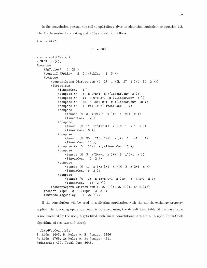
52
In the convolution package the call to splitNest gives an algorithm equivalent to equation 4.2.
The Maple session for creating a size 108 convolution follows:
> n := 4*27;
n := 108
> s := splitNest(n):> SPLPrint(s);(compose
(AgCooleyP 4 27 )(tensorI (RpkInv 2 2 )(RpkInv 3 3 ))(compose
(convert2perm (direct_sum (L 27 1 )(L 27 1 )(L 54 2 )))(direct_sum
(linearConv 1 )(compose (M 3 x^2+x+1 x )(linearConv 2 ))(compose (M 11 x^6+x^3+1 x )(linearConv 6 ))(compose (M 35 x^18+x^9+1 x )(linearConv 18 ))(compose (M 1 x+1 x )(linearConv 1 ))(compose
(tensor (M 3 x^2+x+1 x )(M 1 x+1 x ))(linearConv 2 ))
(compose(tensor (M 11 x^6+x^3+1 x )(M 1 x+1 x ))(linearConv 6 ))
(compose(tensor (M 35 x^18+x^9+1 x )(M 1 x+1 x ))(linearConv 18 ))
(compose (M 3 x^2+1 x )(linearConv 2 ))(compose
(tensor (M 3 x^2+x+1 x )(M 3 x^2+1 x ))(linearConv 2 2 ))
(compose(tensor (M 11 x^6+x^3+1 x )(M 3 x^2+1 x ))(linearConv 6 2 ))
(compose(tensor (M 35 x^18+x^9+1 x )(M 3 x^2+1 x ))(linearConv 18 2 )))
(convert2perm (direct_sum (L 27 27)(L 27 27)(L 54 27))))(tensorI (Rpk 2 2 )(Rpk 3 3 ))(inverse (AgCooleyP 4 27 ))).
If the convolution will be used in a filtering application with the matrix exchange property
applied, the following operation count is obtained using the default hash table (if the hash table
is not modified by the user, it gets filled with linear convolutions that are built upon Toom-Cook
algorithms of size two and three):
> fixedVecCount(s);B Adds: 1407, B Muls: 0, B Assigs: 3866At Adds: 1769, At Muls: 0, At Assigs: 4611Hadamards: 470, Total Ops: 3646.
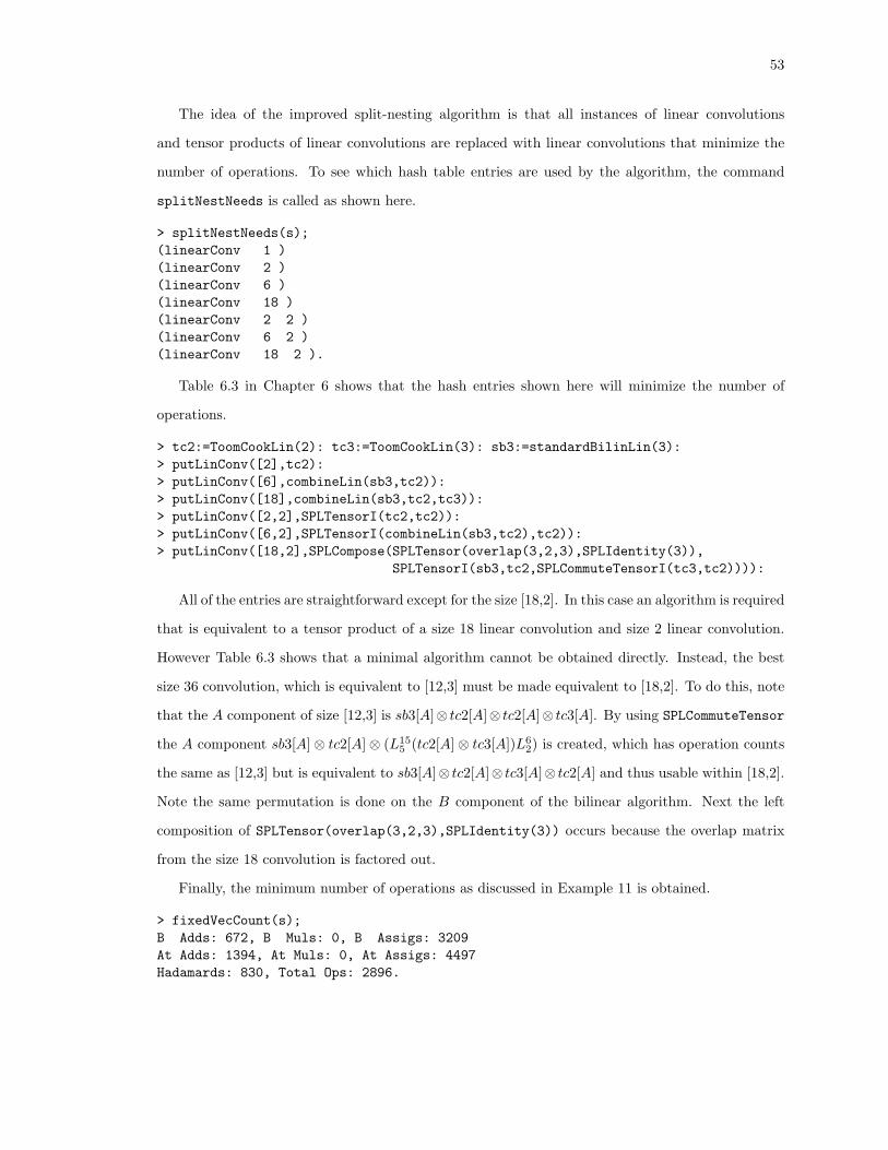
53
The idea of the improved split-nesting algorithm is that all instances of linear convolutions
and tensor products of linear convolutions are replaced with linear convolutions that minimize the
number of operations. To see which hash table entries are used by the algorithm, the command
splitNestNeeds is called as shown here.
> splitNestNeeds(s);(linearConv 1 )(linearConv 2 )(linearConv 6 )(linearConv 18 )(linearConv 2 2 )(linearConv 6 2 )(linearConv 18 2 ).
Table 6.3 in Chapter 6 shows that the hash entries shown here will minimize the number of
operations.
> tc2:=ToomCookLin(2): tc3:=ToomCookLin(3): sb3:=standardBilinLin(3):> putLinConv([2],tc2):> putLinConv([6],combineLin(sb3,tc2)):> putLinConv([18],combineLin(sb3,tc2,tc3)):> putLinConv([2,2],SPLTensorI(tc2,tc2)):> putLinConv([6,2],SPLTensorI(combineLin(sb3,tc2),tc2)):> putLinConv([18,2],SPLCompose(SPLTensor(overlap(3,2,3),SPLIdentity(3)),
SPLTensorI(sb3,tc2,SPLCommuteTensorI(tc3,tc2)))):
All of the entries are straightforward except for the size [18,2]. In this case an algorithm is required
that is equivalent to a tensor product of a size 18 linear convolution and size 2 linear convolution.
However Table 6.3 shows that a minimal algorithm cannot be obtained directly. Instead, the best
size 36 convolution, which is equivalent to [12,3] must be made equivalent to [18,2]. To do this, note
that the A component of size [12,3] is sb3[A]⊗ tc2[A]⊗ tc2[A]⊗ tc3[A]. By using SPLCommuteTensor
the A component sb3[A]⊗ tc2[A]⊗ (L155 (tc2[A]⊗ tc3[A])L6
2) is created, which has operation counts
the same as [12,3] but is equivalent to sb3[A]⊗ tc2[A]⊗ tc3[A]⊗ tc2[A] and thus usable within [18,2].
Note the same permutation is done on the B component of the bilinear algorithm. Next the left
composition of SPLTensor(overlap(3,2,3),SPLIdentity(3)) occurs because the overlap matrix
from the size 18 convolution is factored out.
Finally, the minimum number of operations as discussed in Example 11 is obtained.
> fixedVecCount(s);B Adds: 672, B Muls: 0, B Assigs: 3209At Adds: 1394, At Muls: 0, At Assigs: 4497Hadamards: 830, Total Ops: 2896.
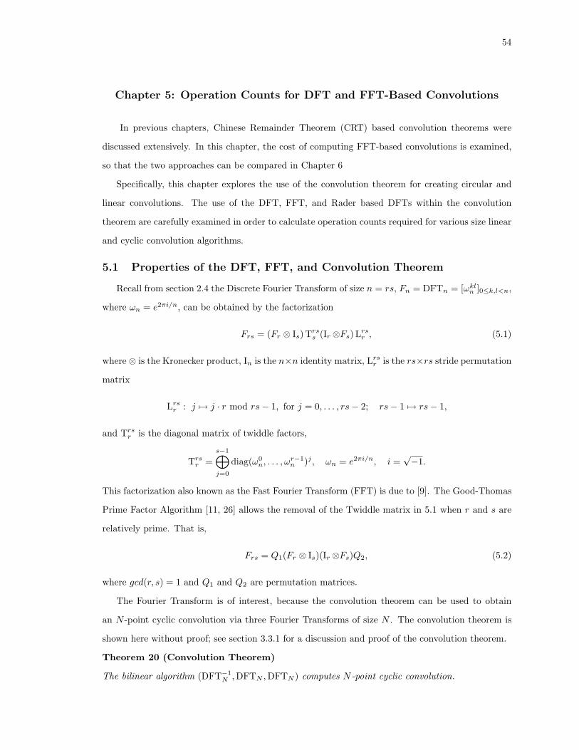
54
Chapter 5: Operation Counts for DFT and FFT-Based Convolutions
In previous chapters, Chinese Remainder Theorem (CRT) based convolution theorems were
discussed extensively. In this chapter, the cost of computing FFT-based convolutions is examined,
so that the two approaches can be compared in Chapter 6
Specifically, this chapter explores the use of the convolution theorem for creating circular and
linear convolutions. The use of the DFT, FFT, and Rader based DFTs within the convolution
theorem are carefully examined in order to calculate operation counts required for various size linear
and cyclic convolution algorithms.
5.1 Properties of the DFT, FFT, and Convolution Theorem
Recall from section 2.4 the Discrete Fourier Transform of size n = rs, Fn = DFTn = [ωkln ]0≤k,l<n,
where ωn = e2πi/n, can be obtained by the factorization
Frs = (Fr ⊗ Is)Trss (Ir ⊗Fs) Lrs
r , (5.1)
where ⊗ is the Kronecker product, In is the n×n identity matrix, Lrsr is the rs×rs stride permutation
matrix
Lrsr : j 7→ j · r mod rs− 1, for j = 0, . . . , rs− 2; rs− 1 7→ rs− 1,
and Trsr is the diagonal matrix of twiddle factors,
Trsr =
s−1⊕
j=0
diag(ω0n, . . . , ωr−1
n )j , ωn = e2πi/n, i =√−1.
This factorization also known as the Fast Fourier Transform (FFT) is due to [9]. The Good-Thomas
Prime Factor Algorithm [11, 26] allows the removal of the Twiddle matrix in 5.1 when r and s are
relatively prime. That is,
Frs = Q1(Fr ⊗ Is)(Ir ⊗Fs)Q2, (5.2)
where gcd(r, s) = 1 and Q1 and Q2 are permutation matrices.
The Fourier Transform is of interest, because the convolution theorem can be used to obtain
an N -point cyclic convolution via three Fourier Transforms of size N . The convolution theorem is
shown here without proof; see section 3.3.1 for a discussion and proof of the convolution theorem.
Theorem 20 (Convolution Theorem)
The bilinear algorithm (DFT−1N , DFTN ,DFTN ) computes N -point cyclic convolution.

55
5.2 DFT and FFT Operation Counts
In order to discuss operation counts, the term “flop” is defined as a single floating point operation
(addition, subtraction, multiplication, or division) between two real numbers. Since complex num-
bers are generally represented in a computer as pairs of real numbers, a multiplication of 2 complex
numbers requires 6 flops (4 multiplications and 2 additions or 3 multiplications and 5 additions) and
the addition of 2 complex numbers requires 2 flops.
From the definition of DFTn above, it is easy to see that the DFTn for a complex vector will
require n2 − n complex additions and (n − 1)2 complex multiplications in general. But it is clear
from (5.1) and (5.2) that the number of operations using the FFT will be:
Lemma 2 Flops(Frs) = s × flops(Fr) + m + r × flops(Fs), with m = 0 when gcd(r, s) = 1 and
m = flops(T rsr ) otherwise.
Note from the definition of the Twiddle matrix that there are no additions required to compute
flops(T rsr ) and that multiplications occur only when ωjk
n is not equal to 1,−1, i, or −i. That is:
Lemma 3 For a complex input vector, flops(T rsr ) = 6((r − 1)(s − 1) − K), and for a real input
vector, flops(T rsr ) = 2((r − 1)(s− 1)−K),
where K = |{(i, j) : 2ijrs ∈ { 1
2 , 1, 32 , 2}, 0 < i ≤ r, 0 < j ≤ s}|.
Example 14 Assuming complex input vectors,
flops(F2) = 4flops(F4) = 2flops(F2) + flops(T 4
2 ) + 2flops(F2)= 8 + 0 + 8= 16
flops(F8) = 2flops(F4) + flops(T 82 ) + 4flops(F2)
= 32 + 12 + 16= 60
flops(F16) = 4flops(F4) + flops(T 164 ) + 4flops(F4)
= 64 + 48 + 64= 176.
5.3 Flop Counts for Rader Algorithm
The FFT factorization gives an algorithm for Frs, but for Fp with p prime the factorization is
of no use. An alternative method for computing Fp for p prime is via Rader’s algorithm [21]. The
basic idea is that given a primitive root r of p, there exist permutation matrices generated by r and

56
r−1 denoted Q(r) and Q(r−1) respectively, such that
Q(r)T FpQ(r−1) =
1 1p−1
1Tp−1 Cp−1
(5.3)
where Cp−1 is a circulant matrix containing the vector w = [ω, ωrp, ωr2
p , . . . , ωrp−2
p ] and 1p−1 is a
1× p− 1 matrix consisting of a single row of ones.
If D = Fp−1w, and Cp−1 = F−1p−1DFp−1, then (5.3) factors into
Q(r)T FpQ(r−1) =
1
F−1p−1
1 1
p− 1 D
1
Fp−1
, (5.4)
and
Flops(Fp) = 2× flops(Fp−1) + 6(p− 1). (5.5)
Example 15 Flops(F17) = 2flops(F16) + 6× 16 = 448. Note that DFT17 by definition would cost
2080 flops.
5.4 Conjugate Even Vectors and Operation Counts
In this section it is shown that Fn operating on a real input vector requires about half of the
computations required to apply Fn to a complex input vector. In order to show this, some terms
need to be defined and some facts proven about the DFT.
Definition 8 (Reflection Matrix)
The reflection matrix En is the n× n matrix defined by
En =
1
Jn−1
where, Jk is the anti-identity matrix defined by
Jk : i 7→ k − 1− i, for j = 0, . . . , k − 1.
Definition 9 (Conjugate Even Vector)
A vector x is called conjugate even if x = Enx.
The next lemma and theorem are modified from [17].
Lemma 4 Fn = EnFn
Proof
Fn = [ωkln ] = [ω−kl
n ] = [ω(n−k)ln ] = EnFn.

57
The following theorem follows directly.
Theorem 21 (Conjugate Even DFT)
Let x be a real vector, then DFTn(x) is conjugate even.
Proof
Since x is real, x = x, so
y = Fn(x) = Fn(x) = Fn(x) = EnFn(x) = Eny.
The implication of Theorem 21 is that when applying a real vector to DFTn, the contents of the
entire output vector are known, after applying only the first n/2 + 1 rows of DFTn. Thus it is not
hard to see that because of the redundancy of the conjugate even vectors, that flops(real DFTn) ≈flops(DFTn)/2.
The symmetry and redundancy of the conjugate even vectors can in fact be exploited by the FFT
as well at the cost of a few extra additions. This was first done by [3] for powers of 2. The method
was refined in [23] also for powers of 2, but can be extended in general for other cases. However for
Rader based Fourier Transforms, it is non-trivial to fully exploit the redundancy for the real case, but
Van Loan in [17] discusses an algorithm whereby two real FFT’s are computed at once, by storing
both into a single complex vector and then using the conjugate even symmetry to separate them. In
this case flops(realFFTn) = flops(FFTn)/2 + n. For comparing operation counts of real vectors
using the convolution theorem versus the CRT methods discussed in Chapter 6 it is reasonable to
use this estimate, since in filtering applications the convolution filter is applied to multiple input
vectors that can be paired up into complex vectors to take advantage of the symmetry.
Table 5.1 shows the flop counts for various size FFT’s and cyclic convolutions. The following
notation is used in Table 5.1 and hereafter.
Notation 1
1. RFn denotes a DFT of size n acting on real inputs.
2. CTn denotes a cyclic convolution of size n computed via the convolution theorem.
3. RCTn denotes a cyclic convolution of size n computed via the convolution theorem and actingon real inputs.
4. FCTn denotes a cyclic convolution of size n computed via the convolution theorem where onevector is fixed.
5. RFCTn denotes a cyclic convolution of size n computed via the convolution theorem whereone vector is fixed, and both vectors are real. (Using the estimate discussed in the precedingparagraph.)

58
Note that flops(FCTn) = 2×flops(Fn)+6×n, but because of the aforementioned symmetries, the
Hadamard products cost half as much in the real case. That is, flops(RFCTn) = 2× flops(RFn)+
3n− 3 + (−1)n+1.
Note that for the small sizes shown in Table 5.1, the asymptotic estimate of 5nLg(n) is not a very
good predictor of the number of operations, particularly for non-power of 2 sizes. Also, notice that
the best FFT-based cyclic convolution of a given size is not always based on an FFT of that size. For
example, for size 23 the convolution theorem would require 3170 flops to convolve 2 complex (1 fixed)
vectors. However, a size 23 cyclic convolution can be obtained from a size 24 linear convolution that
is obtained from a size 48 cyclic convolution from the convolution theorem. With this method, the
size 23 cyclic convolution requires 1984 flops, which is just over half as many as required by using
F23.
Table 5.2 shows ranges of linear convolutions that minimize flop counts. So for example, if a
linear convolution of size between 769 and 800 is needed, it is best created via the convolution
theorem using an FFT of size 1600.
Given the flop counts for linear convolutions provided in Table 5.2, it is now possible to revise
and extend Table 5.1 to show the minimum flop counts for all FFT-based cyclic convolutions of
size 2 through 1024. These are shown in Table 5.3. This table is produced by generating all DFT
factorizations of each size and choosing the one that minimizes operation counts. Note that to save
space, sizes where a linear convolution should be used are omitted; these can be found in Table 5.2.
For example, there is a slight advantage to creating cyclic convolutions of size 28 and 30 directly,
but for a size 29 cyclic convolution, reducing a size 32 linear convolution, derived from a size 64
cyclic convolution minimizes the operation count.
5.5 Summary
This chapter took an extensive look at FFT-based algorithms for linear and cyclic convolu-
tions. The tables discussed in this chapter provide baselines from which the CRT-based algorithms
discussed in previous chapters can be compared.

59
Table 5.1: Flop Counts for various FFT’s and Cyclic Convolutions
Size Flops(Fn) 5nLg(n) Flops(RFn) Flops(FCT n ) Flops(RFCT n )2 4 10 4 20 103 20 24 13 58 334 16 40 12 56 325 56 58 33 142 796 52 78 32 140 787 140 98 77 322 1738 60 120 38 168 969 144 143 81 342 187
10 132 166 76 324 17811 324 190 173 714 37712 128 215 76 328 18413 328 241 177 734 39114 308 267 168 700 37415 268 293 149 626 34116 176 320 104 448 25217 448 347 241 998 53118 324 375 180 756 41019 756 404 397 1626 84920 304 432 172 728 40021 560 461 301 1246 66322 692 491 368 1516 79823 1516 520 781 3170 162924 340 550 194 824 45625 656 580 353 1462 77926 708 611 380 1572 83427 708 642 381 1578 84128 672 673 364 1512 80829 1512 704 785 3198 165530 596 736 328 1372 74231 1372 768 717 2930 152532 488 800 276 1168 64433 1192 832 629 2582 135534 964 865 516 2132 113035 1092 898 581 2394 126536 720 931 396 1656 89637 1656 964 865 3534 183938 1588 997 832 3404 177439 1244 1031 661 2722 143740 748 1064 414 1736 94441 1736 1098 909 3718 193942 1204 1132 644 2660 141043 2660 1167 1373 5578 287344 1472 1201 780 3208 168845 1224 1236 657 2718 144746 3124 1270 1608 6524 335047 6524 1305 3309 13330 675748 848 1340 472 1984 108449 2176 1376 1137 4646 241950 1412 1411 756 3124 165851 1684 1446 893 3674 193752 1520 1482 812 3352 177654 1524 1554 816 3372 179055 2236 1590 1173 4802 250956 1540 1626 826 3416 181657 2648 1662 1381 5638 293160 1312 1772 716 2984 160863 2268 1883 1197 4914 258164 1224 1920 676 2832 1540
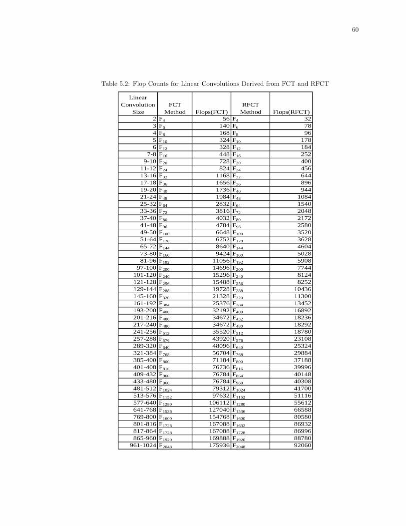
60
Table 5.2: Flop Counts for Linear Convolutions Derived from FCT and RFCT
Linear Convolution
SizeFCT
Method Flops(FCT)RFCT
Method Flops(RFCT)2 F4 56 F4 323 F6 140 F6 784 F8 168 F8 965 F10 324 F10 1786 F12 328 F12 184
7-8 F16 448 F16 2529-10 F20 728 F20 400
11-12 F24 824 F24 45613-16 F32 1168 F32 64417-18 F36 1656 F36 89619-20 F40 1736 F40 94421-24 F48 1984 F48 108425-32 F64 2832 F64 154033-36 F72 3816 F72 204837-40 F80 4032 F80 217241-48 F96 4784 F96 258049-50 F100 6648 F100 352051-64 F128 6752 F128 362865-72 F144 8640 F144 460473-80 F160 9424 F160 502881-96 F192 11056 F192 5908
97-100 F200 14696 F200 7744101-120 F240 15296 F240 8124121-128 F256 15488 F256 8252129-144 F288 19728 F288 10436145-160 F320 21328 F320 11300161-192 F384 25376 F384 13452193-200 F400 32192 F400 16892201-216 F480 34672 F432 18236217-240 F480 34672 F480 18292241-256 F512 35520 F512 18780257-288 F576 43920 F576 23108289-320 F640 48096 F640 25324321-384 F768 56704 F768 29884385-400 F800 71184 F800 37188401-408 F816 76736 F816 39996409-432 F960 76784 F864 40148433-480 F960 76784 F960 40308481-512 F1024 79312 F1024 41700513-576 F1152 97632 F1152 51116577-640 F1280 106112 F1280 55612641-768 F1536 127040 F1536 66588769-800 F1600 154768 F1600 80580801-816 F1728 167088 F1632 86932817-864 F1728 167088 F1728 86996865-960 F1920 169888 F1920 88780
961-1024 F2048 175936 F2048 92060
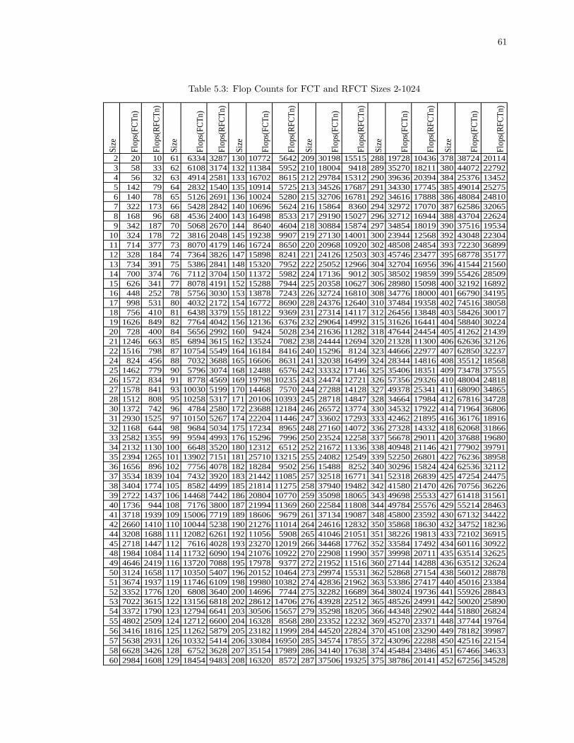
61
Table 5.3: Flop Counts for FCT and RFCT Sizes 2-1024
Size
Flop
s(FC
Tn)
Flop
s(R
FCTn
)
Size
Flop
s(FC
Tn)
Flop
s(R
FCTn
)
Size
Flop
s(FC
Tn)
Flop
s(R
FCTn
)
Size
Flop
s(FC
Tn)
Flop
s(R
FCTn
)
Size
Flop
s(FC
Tn)
Flop
s(R
FCTn
)
Size
Flop
s(FC
Tn)
Flop
s(R
FCTn
)
2 20 10 61 6334 3287 130 10772 5642 209 30198 15515 288 19728 10436 378 38724 201143 58 33 62 6108 3174 132 11384 5952 210 18004 9418 289 35270 18211 380 44072 227924 56 32 63 4914 2581 133 16702 8615 212 29784 15312 290 39636 20394 384 25376 134525 142 79 64 2832 1540 135 10914 5725 213 34526 17687 291 34330 17745 385 49014 252756 140 78 65 5126 2691 136 10024 5280 215 32706 16781 292 34616 17888 386 48084 248107 322 173 66 5428 2842 140 10696 5624 216 15864 8360 294 32972 17070 387 62586 320658 168 96 68 4536 2400 143 16498 8533 217 29190 15027 296 32712 16944 388 43704 226249 342 187 70 5068 2670 144 8640 4604 218 30884 15874 297 34854 18019 390 37516 19534
10 324 178 72 3816 2048 145 19238 9907 219 27130 14001 300 23944 12568 392 43048 2230411 714 377 73 8070 4179 146 16724 8650 220 20968 10920 302 48508 24854 393 72230 3689912 328 184 74 7364 3826 147 15898 8241 221 24126 12503 303 45746 23477 395 68778 3517713 734 391 75 5386 2841 148 15320 7952 222 25052 12966 304 32704 16956 396 41544 2156014 700 374 76 7112 3704 150 11372 5982 224 17136 9012 305 38502 19859 399 55426 2850915 626 341 77 8078 4191 152 15288 7944 225 20358 10627 306 28980 15098 400 32192 1689216 448 252 78 5756 3030 153 13878 7243 226 32724 16810 308 34776 18000 401 66790 3419517 998 531 80 4032 2172 154 16772 8690 228 24376 12640 310 37484 19358 402 74516 3805818 756 410 81 6438 3379 155 18122 9369 231 27314 14117 312 26456 13848 403 58426 3001719 1626 849 82 7764 4042 156 12136 6376 232 29064 14992 315 31626 16441 404 58840 3022420 728 400 84 5656 2992 160 9424 5028 234 21636 11282 318 47644 24454 405 41262 2143921 1246 663 85 6894 3615 162 13524 7082 238 24444 12694 320 21328 11300 406 62636 3212622 1516 798 87 10754 5549 164 16184 8416 240 15296 8124 323 44666 22977 407 62850 3223724 824 456 88 7032 3688 165 16606 8631 241 32038 16499 324 28344 14816 408 35512 1856825 1462 779 90 5796 3074 168 12488 6576 242 33332 17146 325 35406 18351 409 73478 3755526 1572 834 91 8778 4569 169 19798 10235 243 24474 12721 326 57356 29326 410 48004 2481827 1578 841 93 10030 5199 170 14468 7570 244 27288 14128 327 49378 25341 411 68090 3486528 1512 808 95 10258 5317 171 20106 10393 245 28718 14847 328 34664 17984 412 67816 3472830 1372 742 96 4784 2580 172 23688 12184 246 26572 13774 330 34532 17922 414 71964 3680631 2930 1525 97 10150 5267 174 22204 11446 247 33602 17293 333 42462 21895 416 36176 1891632 1168 644 98 9684 5034 175 17234 8965 248 27160 14072 336 27328 14332 418 62068 3186633 2582 1355 99 9594 4993 176 15296 7996 250 23524 12258 337 56678 29011 420 37688 1968034 2132 1130 100 6648 3520 180 12312 6512 252 21672 11336 338 40948 21146 421 77902 3979135 2394 1265 101 13902 7151 181 25710 13215 255 24082 12549 339 52250 26801 422 76236 3895836 1656 896 102 7756 4078 182 18284 9502 256 15488 8252 340 30296 15824 424 62536 3211237 3534 1839 104 7432 3920 183 21442 11085 257 32518 16771 341 52318 26839 425 47254 2447538 3404 1774 105 8582 4499 185 21814 11275 258 37940 19482 342 41580 21470 426 70756 3622639 2722 1437 106 14468 7442 186 20804 10770 259 35098 18065 343 49698 25533 427 61418 3156140 1736 944 108 7176 3800 187 21994 11369 260 22584 11808 344 49784 25576 429 55214 2846341 3718 1939 109 15006 7719 189 18606 9679 261 37134 19087 348 45800 23592 430 67132 3442242 2660 1410 110 10044 5238 190 21276 11014 264 24616 12832 350 35868 18630 432 34752 1823644 3208 1688 111 12082 6261 192 11056 5908 265 41046 21051 351 38226 19813 433 72102 3691545 2718 1447 112 7616 4028 193 23270 12019 266 34468 17762 352 33584 17492 434 60116 3092248 1984 1084 114 11732 6090 194 21076 10922 270 22908 11990 357 39998 20711 435 63514 3262549 4646 2419 116 13720 7088 195 17978 9377 272 21952 11516 360 27144 14288 436 63512 3262450 3124 1658 117 10350 5407 196 20152 10464 273 29974 15531 362 52868 27154 438 56012 2887851 3674 1937 119 11746 6109 198 19980 10382 274 42836 21962 363 53386 27417 440 45016 2338452 3352 1776 120 6808 3640 200 14696 7744 275 32282 16689 364 38024 19736 441 55926 2884353 7022 3615 122 13156 6818 202 28612 14706 276 43928 22512 365 48526 24991 442 50020 2589054 3372 1790 123 12794 6641 203 30506 15657 279 35298 18205 366 44348 22902 444 51880 2682455 4802 2509 124 12712 6600 204 16328 8568 280 23352 12232 369 45270 23371 448 37744 1976456 3416 1816 125 11262 5879 205 23182 11999 284 44520 22824 370 45108 23290 449 78182 3998757 5638 2931 126 10332 5414 206 33084 16950 285 34574 17855 372 43096 22288 450 42516 2215458 6628 3426 128 6752 3628 207 35154 17989 286 34140 17638 374 45484 23486 451 67466 3463360 2984 1608 129 18454 9483 208 16320 8572 287 37506 19325 375 38786 20141 452 67256 34528

62
Table 5.3 (continued))
Size
Flop
s(FC
Tn)
Flop
s(R
FCT
n)
Size
Flop
s(FC
Tn)
Flop
s(R
FCT
n)
Size
Flop
s(FC
Tn)
Flop
s(R
FCT
n)
Size
Flop
s(FC
Tn)
Flop
s(R
FCT
n)
Size
Flop
s(FC
Tn)
Flop
s(R
FCT
n)
Size
Flop
s(FC
Tn)
Flop
s(R
FCT
n)
453 76990 39399 543 84370 43269 632 105368 53944 724 108632 55760 814 128956 66102 909 154206 78919455 54082 27949 544 48528 25348 636 97832 50184 725 117998 60447 815 158386 80821 910 111804 57718456 51944 26880 545 87238 44707 637 92542 47543 726 109676 56286 816 76736 39996 912 110272 56956459 51018 26425 546 62132 32154 640 48096 25324 728 81144 42024 818 150228 76746 915 127706 65681460 77384 39608 548 87864 45024 641 100038 51299 729 88950 45931 819 105210 54241 918 105708 54686462 56476 29158 549 74574 38383 644 119672 61120 730 99972 51442 820 99288 51280 920 161208 82440464 61376 31612 550 66764 34478 645 106718 54647 732 91624 47272 822 139468 71374 924 116648 60168465 60566 31211 552 91720 46960 646 91916 47246 735 95954 49445 824 141400 72344 925 136894 70295468 45144 23504 555 72842 37529 648 61224 31904 736 123888 63412 825 107846 55571 928 130640 67172475 65578 33737 558 72828 37526 650 73412 38002 738 93492 48218 828 147240 75272 930 124852 64282476 50792 26344 560 50624 26428 651 96250 49425 740 93176 48064 832 78800 41060 931 162362 83041477 78462 40183 561 73462 37851 652 117320 59960 741 110686 56823 833 122886 63107 935 130914 67325480 34672 18292 562 99028 50634 654 101372 51990 744 91400 47184 836 127480 65408 936 96840 50288481 70214 36067 565 92206 47231 655 126322 64469 748 93960 48472 837 123006 63175 942 167612 85686482 66004 33962 567 67746 35005 656 73920 38268 750 80572 41782 840 81256 42304 945 114198 58987484 68600 35264 568 93016 47640 657 93654 48139 754 124212 63610 842 159172 81266 948 164056 83920485 61614 31775 570 71428 36850 660 71704 37168 756 80472 41744 843 156410 79889 949 152798 78295486 50892 26414 572 70568 36424 663 81218 41933 760 93464 48248 844 155848 79608 950 134956 69374488 57992 29968 574 77308 39798 665 98406 50531 765 86526 44791 845 117918 60647 952 108248 56024490 59396 30674 576 43920 23108 666 87588 45122 768 56704 29884 847 147154 75269 954 160740 82274492 55112 28536 577 91302 46803 670 130268 66470 769 118022 60547 848 131008 67196 960 76784 40308493 80350 41159 578 72852 37578 671 109202 55941 770 101108 52090 850 97908 50650 962 144276 74058494 69180 35574 579 77530 39921 672 60368 31524 771 107834 55457 852 144920 74160 964 135864 69856495 59058 30517 580 81592 41952 673 124774 63731 772 99256 51168 854 126252 64830 965 137966 70911496 57792 29884 582 70988 36654 674 116052 59370 774 128268 65678 855 119682 61549 968 143976 73920500 49048 25520 584 73320 37824 675 74874 38785 775 113922 58509 858 113860 58642 969 146918 75395504 46872 24440 585 64854 33595 676 84600 43648 776 92840 47968 860 137704 70568 970 127108 65490505 80822 41419 588 68296 35320 678 107212 54958 777 115654 59379 861 123998 63719 972 105672 54776507 66154 34089 589 102542 52447 679 98210 50461 779 132634 67873 864 76848 40148 975 119218 61557510 50204 26118 592 69568 35964 680 65352 34032 780 78152 40632 866 147668 75562 976 122816 63356511 76930 39485 594 72084 37226 682 107364 55042 782 152124 77622 867 117370 60417 980 122712 63312512 35520 18780 595 72058 37217 684 85896 44312 783 127410 65269 868 123704 63584 981 166446 85183513 70806 36427 600 52088 27240 685 119694 61215 784 91584 47356 870 130508 66990 984 117112 60520514 67092 34570 601 107782 55091 686 102140 52438 785 143654 73395 872 133128 68304 986 164644 84290515 92186 47121 602 104580 53490 688 104384 53564 786 147604 75370 873 119286 61387 988 142312 73128516 77944 40000 604 99432 50920 689 126054 64403 790 140716 71934 875 113834 58665 990 122076 63014518 72268 37166 605 94462 48439 690 122516 62634 791 143010 73085 876 115528 59512 992 124016 63988520 48808 25440 606 93916 48166 693 94878 48823 792 88632 45896 880 96192 49852 999 147810 75901522 76356 39218 608 70576 36500 696 96472 49624 793 122358 62763 882 115380 59450 1000 105096 54544524 93512 47800 609 99638 51035 697 99942 51363 795 133738 68457 884 103576 53552 1001 155526 79763525 58702 30399 610 79444 40938 700 74536 38664 798 114044 58614 888 109976 56760 1008 100800 52412527 77586 39845 612 60408 31424 702 79260 41030 800 71184 37188 890 169476 86514 1010 165684 84858528 52928 27516 615 77746 40101 703 123090 62949 801 157014 80107 891 123306 63433 1014 136364 70206530 84212 43162 616 73864 38160 704 72624 37716 802 136788 69994 896 83104 43340 1015 175266 89661532 71064 36592 618 107492 54978 707 125594 64209 803 136074 69641 898 159956 81770 1017 175734 89899533 75230 38679 620 77448 39960 710 124364 63598 804 152248 77728 900 88632 46112 1020 104488 54280534 96844 49486 624 57280 29884 712 127464 65152 805 161182 82199 901 166862 85231 1022 157948 81014536 98104 50120 625 76262 39379 714 82852 42850 806 120076 61646 902 138540 71070 1023 170594 87341539 82858 42505 627 98954 50729 715 98506 50681 808 123336 63280 903 165298 84453 1024 79312 41700540 47976 25064 628 105880 54192 720 59328 31100 810 85764 44498 904 140840 72224541 99198 50679 629 93230 47871 722 129908 66394 812 128520 65880 905 148822 76219542 97052 49606 630 65772 34142 723 105754 54321 813 153166 78207 906 157604 80610

63
Chapter 6: Operation Counts for CRT-Based Convolution Algorithms
In chapter 3 a number of bilinear algorithms based on the constructions of Winograd [29, 30]
and others [19, 27, 1, 22] for computing cyclic and linear convolutions were described. In this
chapter, formulas for counting the operations required for the convolution algorithms discussed in
Chapter 3 will be derived. Operation counts for these algorithms will be compared to the FFT-
based convolution algorithms discussed in Chapter 5. Depending on which components are used
and the order in which the constructions are applied, algorithms with different computational cost
are obtained. Further reduction in cost may be obtained by rearranging the factors in the algorithm
using properties of the tensor product and other algebraic manipulations.
The set of algorithms that can be obtained from these constructions defines a space of convolution
algorithms, and for a given size finding the algorithm in the space with minimal cost becomes a well
defined optimization problem. In this chapter, operation count is used as the cost function since it
provides exact results and is easy to compare with previous work. However, using the automated
algorithm generation and implementation outlined in Section 4.1, a similar optimization problem
can be carried out using runtime for the cost function. This will be discussed in chapter 7.
6.1 Assumptions and Methodology
The assumptions used for this chapter are as follows. It is assumed that the ultimate goal is to
calculate circular convolutions on pairs of real and complex vectors (one fixed) via matrix exchange.
Linear convolutions were discussed in chapter 3, but the reason for introducing linear convolutions
was their utility within circular convolutions. The aim is in minimizing the total number of additions
and multiplications and not to minimize multiplications at the expense of additions since for many
modern architectures the costs are the same. Finally, all multiplications are counted, and not just
the ones that occur in the diagonal matrix in the matrix exchange procedure. The multiplication
count is kept as two separate tallies, those due to the diagonal matrix plus all others, since the
former can not be avoided, while the latter can sometimes be removed via shifts or other means,
particularly on integer inputs.
The following notation is used throughout the chapter.

64
Notation 2
1. flops(X) denotes the number of floating point operations required to evaluate an expression.
2. multiplications(X) denotes the number of multiplications required to evaluate an expression.Note that each real multiplication requires 1 flop and each complex multiplication requires 6flops (4 multiplications and 2 additions, or 3 multiplications and 3 additions).
3. adds(X) denotes the number of adds required to evaluate an expression. Note that each realadd requires 1 flop and each complex add requires 2 flops.
4. rowdim(M) denotes the number of rows in the matrix M .
5. coldim(M) denotes the number of columns in a matrix M .
The following theorem summarizing the cost of applying the direct sum and tensor product of two
matrices given the costs of the individual matrices, will also be needed throughout the chapter.
Theorem 22 (Cost of the Direct Sum and Tensor Product) Let A be a matrix requiring
adds(A) additions and multiplications(A) multiplications to apply a vector. Let B be a matrix
requiring adds(B) additions and multiplications(B) multiplications to apply a vector. Then
1. A ⊕ B can be applied to a vector using adds(A ⊕ B) = adds(A) + adds(B) additions andmultiplications(A⊕B) = multiplications(A) + multiplications(B) multiplications.
2. A⊗B can be applied to a vector using coldim(A)×adds(B)+rowdim(B)×adds(A) additionsand coldim(A)×multiplications(B) + rowdim(B)×multiplications(A) multiplications.
Proof
The result for the direct sum is obvious and the result for the tensor product follows from the
factorization A ⊗ B = (A ⊗ Irowdim(B))(Icoldim(A) ⊗ B), and the commutation theorem, which
implies that up to a permutation (A ⊗ Irowdim(B)) is equal to (Irowdim(B) ⊗ A). If A and B are
rectangular matrices, the number of operations for A ⊗ B is not the same as for B ⊗ A using this
factorization.
6.2 Operation Counts for Size p (p prime) Linear Convolutions Embeddedin Circular Convolutions
Definition 10 A bilinear algorithm for a k-size linear convolution is defined as (C,A, B)<k> or
(C<k>, A<k>, B<k>).
Let (C, A,B)<p> be a bilinear algorithm for a linear convolution. If this algorithm will be em-
bedded into an algorithm for computing circular convolutions, then because of the matrix exchange
property, the number of operations required to convolve 2 vectors via (C,A, B)<p> will be the

65
number of additions and multiplications required for applying vectors to B<p> and AT<p>, plus the
rowdim(B<p>) multiplications for the diagonal matrix created by matrix exchange. This can be
defined more precisely for the real and complex case as follows:
Theorem 23 Let (C,A, B)<p> be a bilinear algorithm for a linear convolution to be embedded in
a cyclic convolution where matrix exchange is to be applied. If the vectors to be convolved are real,
then
flops(C, A,B)<p>) = flops(B<p>) + flops(AT<p>) + rowdim(B<p>) (6.1)
If the vectors to be convolved are complex, then
flops(C, A, B)<p>) = flops(B<p>) + flops(AT<p>) + 6× rowdim(B<p>) (6.2)
Example 16 In Example 5 of chapter 3 a 3×3 linear convolution given by the Toom-Cook algorithmwas shown to be:
tc3 =
1 0 0 0 0−1/2 1 −1/3 −1/6 2−1 1/2 1/2 0 −11/2 −1/2 −1/6 1/6 −2
0 0 0 0 1
,
1 0 01 1 11 −1 11 2 40 0 1
,
1 0 01 1 11 −1 11 2 40 0 1
= (tc3[C], tc3[A], tc3[B])
The operation count for this algorithm can be reduced using the following factorization.
1 0 01 1 11 −1 11 2 40 0 1
=
1 0 0 0 0 00 1 0 0 0 01 0 1 0 0 00 1 1 1 1 00 0 0 0 0 1
1 0 0 01 1 0 00 0 1 00 1 0 00 1 0 00 0 0 1
1 0 00 1 10 −1 10 0 1
The number of operations required by this algorithm to convolve complex vectors is
flops(tc3) = flops(tc3[At]) + flops(tc3[B]) + 6× rowdim(tc3[B])= 2× 9 + 2× 7 + 6× 5= 62.
6.3 Operation Counts for Size mn Linear ConvolutionsEmbedded in Circular Convolutions
Let Lm and Ln be bilinear algorithms for computing linear convolutions of size m and n
respectively. It was shown in section 3.1.3 that a linear convolution algorithm of size mn is
Om,n(Lm⊗Ln) = (Om,nCm⊗Cn, Am⊗An, Bm⊗Bn). Since Om,n is part of the C component, when
embedding the linear algorithm into a cyclic convolution and using matrix exchange, the number of
operations is flops(ATm ⊗ AT
n ) + flops(Bm ⊗ Bn) + d, where d = 6 × rowdim(Bm) × rowdim(Bn)

66
in the case of complex inputs or d = rowdim(Bm) × rowdim(Bn) in the case of real inputs. The
d operations come from the multiplications required when applying a vector to the precomputed
diagonal matrix obtained from matrix exchange. Thus, using Theorem 22,
flops(Lmn) = flops(Lm ⊗ Ln)= flops(AT
m ⊗ATn ) + flops(Bm ⊗Bn) + d
= coldim(Am)× adds(ATn ) + rowdim(An)× adds(AT
m)+coldim(Am)×multiplications(AT
n ) + rowdim(An)×multiplications(ATm)
+coldim(Bm)× adds(Bn) + rowdim(Bn)× adds(Bm)+coldim(Bm)×multiplications(Bn) + rowdim(Bn)×multiplications(Bm) + d
= m× adds(ATn ) + rowdim(Bn)× adds(AT
m)+m×multiplications(AT
n ) + rowdim(Bn)×multiplications(ATm)
+m× adds(Bn) + rowdim(Bn)× adds(Bm)+m×multiplications(Bn) + rowdim(Bn)×multiplications(Bm) + d
= m(flops(ATn ) + flops(Bn)) + rowdim(Bn)(flops(AT
m) + flops(Bm)) + d.
This result is summarized in the following theorem.
Theorem 24 (Operation Counts for Combining Linear Convolutions)
Let Lm = (Cm, Am, Bm) and Ln = (Cn, An, Bn) be linear convolutions of size m and n respectively.
These can be combined via a tensor product to form a linear convolution of size mn. Assuming
this linear convolution will be embedded into a cyclic convolution where matrix exchange will be used
then, if the vectors are real, the number of operations is
flops(Lmn) = m(flops(ATn ) + flops(Bn)) + rowdim(Bn)(flops(AT
m)+flops(Bm)) + rowdim(Bm)× rowdim(Bn).
If the vectors to be convolved are complex, the number of operations is
flops(Lmn) = 2m(flops(ATn ) + flops(Bn)) + 2× rowdim(Bn)(flops(AT
m)+flops(Bm)) + 6× rowdim(Bm)× rowdim(Bn).
Unfortunately, there is no closed form formula for counting the number of operations required
for computing linear convolutions of arbitrary size, since there are multiple ways to compute any
linear convolution, and even more ways to combine arbitrary convolutions to make larger ones. For
example, the 5-point linear convolution can be created by definition, via a 6-point linear convolution,
via an 8-point linear convolution, or via an 8-point circular convolution (each of which can in turn
be computed multiple ways).
67
Although there is no single formula for calculating the operation counts, Theorems 23 and 24
do provide a means of finding optimal algorithms via an exhaustive search. The idea is to compute
linear convolutions via each of the methods presented in chapter 3 for prime sizes 2 through 29 and
then to search for the best way of combining these algorithms using the tensor product to obtain the
best algorithm for all sizes through 1024. Table 6.1 shows the operation counts for various prime
sizes 2 through 29.
The shorthand used in Table 6.1 is as follows: tp is a size p convolution computed via the Toom-
Cook algorithm, sp is a size p convolution computed via the standard algorithm, kLp is a size p
convolution compute reduced from a linear convolution of size k, and kcp is a size p convolution
computed via a cyclic convolution of size k. Note that if there are multiple ways of computing any
algorithm, each is differentiated via an a,b,c etc.
The table shows the algorithms that remain after algorithms that are guaranteed not to be
optimal have been pruned. As an example it is possible to create a 3-point linear convolution via a
4-point linear convolution. However, since this algorithm would use as many diagonal multiplications
as 4c3, plus as many or more operations in both the AT , and B components, it is clear that it would
require more operations as a standalone 3-point linear convolution algorithm, but more importantly,
would have no chance of being part of a larger optimum algorithm.
Combining Table 6.1 and Theorem 24 gives a method to calculate the operations required for
any combination of the algorithms shown in Table 6.1. There is still a significant search problem
however, since there are many ways of combining linear convolutions and since Lx ⊗ Ly will often
require a different number of operations than Ly ⊗ Lx. As an example, consider Table 6.2 showing
16 different ways to compute a convolution of size 6. Similarly there are 384 ways to compute a
36-point linear convolution, 512 ways to compute a 54-point linear convolution and so on. Note that
the best algorithm for convolving real vectors is not the best for convolving complex vectors.
Just as all combinations of algorithms that yield size 6 convolutions were shown in Table 6.2,
a similar table could be created for any size from 2 to 1024. From that table, the algorithm that
minimized the number of operations could be chosen. There are more than 1.6 million different
algorithm combinations for computing all possible linear convolutions through 1024. The combina-
tions that minimize operation counts for real vectors are shown in Table 6.3. The combinations that
minimize operations for complex vectors are shown in Table 6.4.

68
Table 6.1: Operation Counts for P-Point Linear Convolutions
Total TotalRowdim(B) Flops Flops
Diagonal Real Complex
P Method Adds(B) Multiplies(B) Adds(AT) Multiplies(AT) Multiplies Inputs Inputs2 s2 0 0 2 0 4 6 282 t2 1 0 2 0 3 6 243 4c3 4 0 7 0 6 17 583 4l3 4 0 9 0 9 22 803 s3 0 0 6 0 9 15 663 t3 7 0 9 0 5 21 625 8c5 14 0 22 0 13 49 1505 s5 0 0 20 0 25 45 1905 t5 19 12 23 12 9 75 1867 12c7a 44 0 58 0 21 123 3307 12c7b 25 0 43 0 25 93 2867 12c7c 34 7 49 7 22 119 3267 12c7d 38 7 52 7 21 125 3347 8L7 19 0 38 0 27 84 2767 s7 0 0 42 0 49 91 3787 t7 41 30 47 30 13 161 374
11 12La11 60 0 102 0 54 216 64811 12Lb11 63 0 96 0 45 204 58811 20c11a 86 0 117 0 42 245 65811 20c11b 76 0 108 0 43 227 62611 20c11c 59 0 94 0 46 199 58211 s11 0 0 110 0 121 231 94611 t11 109 90 119 90 21 429 94213 14L13a 109 0 188 0 63 360 97213 14L13b 49 0 140 0 147 336 126013 14L13c 75 0 143 0 75 293 88613 14L13d 133 0 155 0 65 353 96613 16L13 65 0 130 0 81 276 87613 24c13 128 0 172 0 57 357 94213 s13 0 0 156 0 169 325 132613 t13 155 132 167 132 25 611 132217 t17 271 240 287 240 33 1071 227423 t23 505 462 527 462 45 2001 418229 t29 811 756 839 756 57 3219 6666
(Assumed to be Embedded in Cyclic Convolutions using Matrix Exchange and 1 fixed Vector)
6.4 Operation Counts for Any Size Cyclic Convolution
In this section, a formula for counting operations for any size cyclic convolution will be pre-
sented. Recall from section 3.3.4 that any size cyclic convolution could be constructed by combining
prime power cyclic convolutions via the split-nesting algorithm. Let
Ckp = R−1
pk
(k⊕
i=0
M(Φpi(x)Lφ(pi)
)Rpk
be a prime power cyclic convolution, and let N = pk11 pk2
2 . . . pkl
l , then
CN = Q−1
(l⊗
i=1
R−1
pkii
)(l⊗
i=1
Cp
kii
)(l⊗
i=1
Rp
kii
)Q (6.3)

69
Table 6.2: Different Methods for Computing 6-Point Linear Convolutions
Total TotalRowdim(B) Flops FlopsDiagonal Real Complex
Method Adds(B) Multiplies(B) Adds(AT) Multiplies(AT) Multiplies Inputs Inputss3⊗t2 3 0 24 0 27 54 216t2⊗4c3 14 0 26 0 18 58 188s2⊗4c3 8 0 26 0 24 58 2124c3⊗t2 15 0 27 0 18 60 192t2⊗t3 19 0 28 0 15 62 184s3⊗s2 0 0 30 0 36 66 276s2⊗s3 0 0 30 0 36 66 276s2⊗t3 0 0 30 0 36 66 276t2⊗s3 9 0 30 0 27 66 240t3⊗t2 24 0 33 0 15 72 2044c3⊗s2 16 0 34 0 24 74 2444L3⊗t2 15 0 33 0 27 75 258t2⊗4L3 17 0 36 0 27 80 268s2⊗4L3 8 0 36 0 36 80 304t3⊗s2 28 0 42 0 20 90 2604L3⊗s2 16 0 42 0 36 94 332
is an N -point cyclic convolution via the Agarwal-Cooley algorithm. (Note that Q and Q−1 are
permutation matrices defined in section 3.3.4.) Now by the split-nesting algorithm,
l⊗
i=1
Cp
kii
=P1
(k1⊕
i1=0
k2⊕
i2=0
. . .
kl⊕
il=0
Φpi1 (x)Lφ(pi1 ) ⊗ Φpi2 (x)Lφ(pi2 ) ⊗ . . .⊗ Φpil (x)Lφ(pil )
)P2,
where P1 and P2 are permutation matrices as defined in section 3.3.4. Since permutation matrices
cost 0 operations, and since the reduction matrices are precomputed via matrix exchange, it follows
that
flops
(l⊗
i=1
Cp
kii
)= flops
(k1⊕
i1=0
k2⊕
i2=0
. . .
kl⊕
il=0
Lφ(pi1 ) ⊗ Lφ(pi2 ) ⊗ . . .⊗ Lφ(pil )
)
= flops
(k1⊕
i1=0
k2⊕
i2=0
. . .
kl⊕
il=0
Lφ(pi1 )φ(pi2 )...φ(pil )
)
=k1∑
i1=0
k2∑
i2=0
. . .
kl∑
il=0
flops(Lφ(pi1 )φ(pi2 )...φ(pil )). (6.4)
Rpk and RTpk require 2(pk − 1) additions each; this is easily seen by an induction on the factor-
ization of Rpk provided in Theorem 16. It follows that
flops
(l⊗
i=1
Rp
kii
)= flops
(l⊗
i=1
Rp
kii
)T
=l∑
i=1
pk11 pk2
2 . . . pkl
l
pkii
2(pkii − 1) additions. (6.5)

70
Note that the operations required for ⊗li=1R
−1
pkii
can be derived in a similar manner; however,
because of matrix exchange, they are not included in the cost of the convolution.
The following theorem follows directly from (6.3), (6.4), and (6.5).
Theorem 25 (Operation Counts for Size N Cyclic Convolution)
Let N = pk11 pk2
2 . . . pkl
l , and let CN be a size N cyclic convolution. If the vectors to be convolved are
real, then
flops(CN ) =k1∑
i1=0
k2∑
i2=0
. . .
kl∑
il=0
flops(Lφ(pi1 )φ(pi2 )...φ(pil )) + 4l∑
i=1
pk11 pk2
2 . . . pkl
l
pkii
(pkii − 1).
If the vectors to be convolved are complex, then
flops(CN ) =k1∑
i1=0
k2∑
i2=0
. . .
kl∑
il=0
flops(Lφ(pi1 )φ(pi2 )...φ(pil )) + 8l∑
i=1
pk11 pk2
2 . . . pkl
l
pkii
(pkii − 1).
Proof
From (6.3),
flops(CN ) = flops
(l⊗
i=1
Cp
kii
)+ flops
(l⊗
i=1
Rp
kii
)+ flops
(l⊗
i=1
Rp
kii
)T .
The formulas now follow from (6.4), and (6.5).
Example 17 To compute the cost of a size 108 cyclic convolution on real vectors using matrix
exchange and one fixed vector, observe that 108 = 22 × 33. From Theorem 25 and Table 6.3, it
follows that
flops(C108) = flops(Lφ(1)) + flops(Lφ(3)) + flops(Lφ(9)) + flops(Lφ(27))
+flops(Lφ(2)) + flops(Lφ(6)) + flops(Lφ(18)) + flops(Lφ(54))
+flops(Lφ(4)) + flops(Lφ(12)) + flops(Lφ(36)) + flops(Lφ(108))
+4(27× 3 + 4× 26)
= flops(L1) + flops(L2) + flops(L6) + flops(L18)
+flops(L1) + flops(L2) + flops(L6) + flops(L18)
+flops(L2) + flops(L4) + flops(L12) + flops(L36) + 740
= 1 + 6 + 54 + 366 + 1 + 6 + 54 + 366 + 6 + 24 + 180 + 1092 + 740
= 2896.
The use of the improved split-nesting algorithm in this case saves 120 operations over the method
published in [22].

71
Operation counts of cyclic convolutions for most sizes through 1000 are shown in Table 6.5.
This table compares the improved split-nesting costs with the FFT-based cyclic convolution costs
presented in chapter 5. In order to conserve space, the improved split-nesting counts show the
difference between the convolution theorem counts rather than actual counts. For example, for real
inputs, the split-nesting algorithm of size two uses four fewer flops than the ten required for the
FFT-based convolution theorem algorithm of size two. The cases where the improved split-nesting
algorithm uses fewer operations are noted in gray.
Also to conserve space all sizes that contain a prime factor equal or greater than 29 are removed.
As a rule, these sizes tend to be poor choices for either algorithm, (reduced larger composite sizes can
be used), although the improved split-nesting algorithm uses fewer operations in general for these
sizes. Specifically, for convolutions on real inputs the improved split-nesting algorithm uses fewer
operations for about 90% of the sizes between 2 and 200 and more than half the sizes between 2 and
500. Beyond that, the FFT-based algorithms outperform the CRT-based algorithms in general. For
complex inputs, the window is much smaller. The CRT-based algorithms outperform the FFT-based
methods for only 48% of the sizes between 2 and 100, and even less for larger sizes.
Figure 6.1 illustrates how the improved split-nesting algorithm performs in various size ranges
for both real and complex inputs.
6.5 Mixed Algorithms for Cyclic Convolutions
Table 6.5 shows that the improved split-nesting algorithm uses fewer operations than the
FFT-based algorithm in many cases, but the counts can often be further improved by computing
the convolution partially via the improved split-nesting algorithm and partially via the FFT. This
is generally the case for size N = mn, where the improved split-nesting algorithm is optimal for size
m and the convolution theorem using the FFT is optimal for size n. This occurs for many cases
when N = m · 2k.
By the mixed convolution theorem (Theorem 14), a size mn cyclic convolution can be created via
a size m cyclic convolution constructed from the convolution theorem and a size n cyclic convolution
constructed from the CRT methods. The following theorem quantifies the savings from mixing
algorithms compared to using the convolution theorem.
Theorem 26 (Mixed Complex Cyclic Convolution Count Savings)
Let ctm = (F−1m , Fm, Fm) and snm = (Cm, Am, Bm) be cyclic convolutions of size m based on the
convolution theorem and the CRT respectively. Suppose one vector is fixed and matrix exchange is
used, and snm uses k fewer operations than ctm (that is flops(ctm) = flops(snm)+k). Then a size

72
mn convolution created by the mixed convolution theorem (Theorem 14), will use at least nk fewer
operations than a size mn convolution created via the convolution theorem.
Proof
Let U1 be the CRT-based convolution algorithm of size m after matrix exchange is applied, and let
U2 be an FFT-based convolution algorithm of size m after matrix exchange is applied, so that
U1 = JmAT1 D1B1
U2 = JmFmD2Fm,
with, D1 = CT1 Jmv1 and D2 = F−1
m Jmv2.
By the statement of the theorem flops(U2) = flops(U1) + k. Now let W1 be a mixed algorithm
of size mn and let W2 be an FFT-based convolution theorem algorithm of size mn. That is
W1 = Jmn(Fn ⊗ Im)(In ⊗AT1 )D′
1(In ⊗B1)(Fn ⊗ Im)
W2 = JmnFmnD′2Fmn
= Jmn(Fn ⊗ Im)Tmnm (In ⊗ Fm)D′
2(In ⊗ Fm)Tmnm (Fn ⊗ Im).
Now, observe that flops(D′1) = n · flops(D1) and flops(D′
2) = n · flops(D2) and also
flops(Jmn) = n · flops(Jm) = 0. Also note that, flops((In ⊗ AT )D′1(In ⊗ B1)) = n · flops(U1).
Similarly, flops((In ⊗ Fm)D′2(In ⊗ Fm)) = n · flops(U2). Thus
flops(W1) = 2m · flops(Fn) + n · flops(U1)
flops(W2) = 2m · flops(Fn) + 2 · flops(Tmnm ) + n · flops(U2)
= 2m · flops(Fn) + 2 · flops(Tmnm ) + n · (flops(U1) + k).
It follows that flops(W2) = flops(W1)+2 · flops(Tmnm )+nk. (Note that the 2 · flops(Tmn
n ) can
be avoided by choosing a factorization so that gcd(m, n) = 1 as discussed in chapter 5.) Thus the
initial advantage increases with the size of n.
Note that when the inputs are real, a similar Theorem exists, but the advantage is less significant
since at least part of smn will act on complex vectors.
Example 18 From Tables 5.1 and 6.5 and Theorem 26, the cost of the size 112 = 7×16 convolution
on complex inputs is 16× 238 + 2× 7× 176 = 6272 operations. The 6272 operations for the mixed
convolution are considerably fewer than the 7616 operations required by a pure FFT solution or the
9448 operations required by the improved split-nesting algorithm. Moreover, the operation count
advantage will increase for size 224 = 7× 32, size 448 = 7× 64 and so on.

73
Table 6.3: Linear Convolutions that Minimize Operations for Real Inputs
Size Method Flops Size Method Flops2 t2 6 169-180 s3⊗t2⊗t2⊗t3⊗t5 122043 s3 15 181-189 s3⊗t3⊗t3⊗t7 138634 t2⊗t2 24 190-200 t2⊗t2⊗t2⊗t5⊗t5 141965 s5 45 201-210 s3⊗t2⊗t5⊗t7 159066 s3⊗t2 54 211-224 t2⊗t2⊗t2⊗t2⊗t2⊗t7 16124
7-8 t2⊗t2⊗t2 84 225-240 t2⊗t2⊗t2⊗t2⊗t3⊗t5 178929 s3⊗t3 123 241-252 s3⊗t2⊗t2⊗t3⊗t7 19524
10 t2⊗8c5 150 253-264 t2⊗t2⊗t2⊗t3⊗t11 2130011-12 s3⊗t2⊗t2 180 265-280 t2⊗t2⊗t2⊗t5⊗t7 2261213-14 8L7⊗t2 273 281-300 s3⊗t2⊗t2⊗t5⊗t5 2566815-16 t2⊗t2⊗t2⊗t2 276 301-312 t2⊗t2⊗t2⊗t3⊗t13 2776417-18 s3⊗t2⊗t3 366 313-336 t2⊗t2⊗t2⊗t2⊗t3⊗t7 2837219-20 t2⊗t2⊗8c5 456 337-352 t2⊗t2⊗t2⊗t2⊗t2⊗t11 31452
21 8L7⊗t3 532 353-360 t2⊗t2⊗t2⊗t3⊗t3⊗t5 3286822-24 t2⊗t2⊗t2⊗t3 548 361-378 s3⊗t2⊗t3⊗t3⊗t7 35526
25 s5⊗t5 735 379-400 t2⊗t2⊗t2⊗t2⊗t5⊗t5 3714026-27 s3⊗t3⊗t3 759 401-420 s3⊗t2⊗t2⊗t5⊗t7 40236
28 8L7⊗t2⊗t2 861 421-440 t2⊗t2⊗t2⊗t5⊗t11 4328429-32 t2⊗t2⊗t2⊗t2⊗t2 876 441-448 t2⊗t2⊗t2⊗t2⊗t2⊗t2⊗t7 4488433-36 s3⊗t2⊗t2⊗t3 1092 449-450 s3⊗t2⊗t3⊗t5⊗t5 4627837-40 t2⊗t2⊗t2⊗t5 1284 451-468 s3⊗t2⊗t2⊗t3⊗t13 4839641-42 8L7⊗t2⊗t3 1589 469-480 t2⊗t2⊗t2⊗t2⊗t2⊗t3⊗t5 5036443-48 t2⊗t2⊗t2⊗t2⊗t3 1636 481-504 t2⊗t2⊗t2⊗t3⊗t3⊗t7 5126849-50 t2⊗8c5⊗t5 2010 505-528 t2⊗t2⊗t2⊗t2⊗t3⊗t11 5394051-54 s3⊗t2⊗t3⊗t3 2118 529-560 t2⊗t2⊗t2⊗t2⊗t5⊗t7 5786055-56 t2⊗t2⊗t2⊗t7 2276 561-588 s3⊗t2⊗t2⊗t7⊗t7 6594057-60 s3⊗t2⊗t2⊗t5 2412 589-594 s3⊗t2⊗t3⊗t3⊗t11 6651061-64 t2⊗t2⊗t2⊗t2⊗t2⊗t2 2724 595-600 t2⊗t2⊗t2⊗t3⊗t5⊗t5 6656465-72 t2⊗t2⊗t2⊗t3⊗t3 3124 601-624 t2⊗t2⊗t2⊗t2⊗t3⊗t13 6902873-80 t2⊗t2⊗t2⊗t2⊗t5 3540 625-630 s3⊗t2⊗t3⊗t5⊗t7 7158681-84 s3⊗t2⊗t2⊗t7 4116 631-660 s3⊗t2⊗t2⊗t5⊗t11 7513285-90 s3⊗t2⊗t3⊗t5 4482 661-672 t2⊗t2⊗t2⊗t2⊗t2⊗t3⊗t7 7780491-96 t2⊗t2⊗t2⊗t2⊗t2⊗t3 4892 673-704 t2⊗t2⊗t2⊗t2⊗t2⊗t2⊗t11 83316
97-100 t2⊗t2⊗8c5⊗t5 5424 705-728 t2⊗t2⊗t2⊗t7⊗t13 89716101-112 t2⊗t2⊗t2⊗t2⊗t7 5956 729-784 t2⊗t2⊗t2⊗t2⊗t7⊗t7 94004113-120 t2⊗t2⊗t2⊗t3⊗t5 6516 785-792 t2⊗t2⊗t2⊗t3⊗t3⊗t11 94980121-126 s3⊗t2⊗t3⊗t7 7422 793-800 t2⊗t2⊗t2⊗t2⊗t2⊗t5⊗t5 100524127-128 t2⊗t2⊗t2⊗t2⊗t2⊗t2⊗t2 8364 801-840 t2⊗t2⊗t2⊗t3⊗t5⊗t7 102468129-135 s3⊗t3⊗t3⊗t5 8613 841-880 t2⊗t2⊗t2⊗t2⊗t5⊗t11 106980136-140 t2⊗t2⊗8c5⊗t7 8888 881-882 s3⊗t2⊗t3⊗t7⊗t7 115134141-144 t2⊗t2⊗t2⊗t2⊗t3⊗t3 8948 883-936 t2⊗t2⊗t2⊗t3⊗t3⊗t13 120292145-150 s3⊗t2⊗t5⊗t5 9918 937-990 s3⊗t2⊗t3⊗t5⊗t11 130842151-160 t2⊗t2⊗t2⊗t2⊗t2⊗t5 9996 991-1040 t2⊗t2⊗t2⊗t2⊗t5⊗t13 135380161-168 t2⊗t2⊗t2⊗t3⊗t7 10676
(Assumed to be Embedded in Circular Convolutions with Matrix Exchange Applied to one Fixed Input)

74
Table 6.4: Linear Convolutions that Minimize Operations for Complex Inputs
Size Method Flops Size Method Flops2 t2 24 209-210 t2⊗t3⊗t5⊗t7 407043 4c3 58 211-220 t2⊗t2⊗t5⊗t11 432844 t2⊗t2 84 221-224 t2⊗t2⊗t2⊗t2⊗t2⊗t7 448845 8c5 150 225 4c3⊗t3⊗t5⊗t5 478986 t2⊗t3 184 226-234 t2⊗t3⊗t3⊗t13 48896
7-8 t2⊗t2⊗t2 276 235-240 t2⊗t2⊗t2⊗t2⊗t3⊗t5 503649 4c3⊗t3 386 241-252 t2⊗t2⊗t3⊗t3⊗t7 51268
10 t2⊗8c5 456 253-264 t2⊗t2⊗t2⊗t3⊗t11 5394011-12 t2⊗t2⊗t3 548 265-280 t2⊗t2⊗t2⊗t5⊗t7 5786013-14 8L7⊗t2 870 281-300 t2⊗t2⊗t3⊗t5⊗t5 6656415-16 t2⊗t2⊗t2⊗t2 876 301-312 t2⊗t2⊗t2⊗t3⊗t13 6902817-18 t2⊗t3⊗t3 1112 313-315 4c3⊗t3⊗t5⊗t7 7392619-20 t2⊗t2⊗t5 1284 316-330 t2⊗t3⊗t5⊗t11 75888
21 8L7⊗t3 1604 331-336 t2⊗t2⊗t2⊗t2⊗t3⊗t7 7780422-24 t2⊗t2⊗t2⊗t3 1636 337-352 t2⊗t2⊗t2⊗t2⊗t2⊗t11 83316
25 8c5⊗t5 2010 353-364 t2⊗t2⊗t7⊗t13 8971626-27 4c3⊗t3⊗t3 2218 365-392 t2⊗t2⊗t2⊗t7⊗t7 94004
28 t2⊗t2⊗t7 2276 393-396 t2⊗t2⊗t3⊗t3⊗t11 9498029-30 t2⊗t3⊗t5 2448 397-400 t2⊗t2⊗t2⊗t2⊗t5⊗t5 10052431-32 t2⊗t2⊗t2⊗t2⊗t2 2724 401-420 t2⊗t2⊗t3⊗t5⊗t7 10246833-36 t2⊗t2⊗t3⊗t3 3124 421-440 t2⊗t2⊗t2⊗t5⊗t11 10698037-40 t2⊗t2⊗t2⊗t5 3540 441 4c3⊗t3⊗t7⊗t7 11851441-42 t2⊗t3⊗t7 4168 442-468 t2⊗t2⊗t3⊗t3⊗t13 12029243-45 4c3⊗t3⊗t5 4662 469-476 t2⊗t2⊗t7⊗t17 13323646-48 t2⊗t2⊗t2⊗t2⊗t3 4892 477-495 4c3⊗t3⊗t5⊗t11 13462249-50 t2⊗8c5⊗t5 5424 496-520 t2⊗t2⊗t2⊗t5⊗t13 13538051-56 t2⊗t2⊗t2⊗t7 5956 521-528 t2⊗t2⊗t2⊗t2⊗t3⊗t11 14190057-60 t2⊗t2⊗t3⊗t5 6516 529-546 t2⊗t3⊗t7⊗t13 15342461-63 4c3⊗t3⊗t7 7682 547-560 t2⊗t2⊗t2⊗t2⊗t5⊗t7 153628
64 t2⊗t2⊗t2⊗t2⊗t2⊗t2 8364 561-588 t2⊗t2⊗t3⊗t7⊗t7 16365265-66 t2⊗t3⊗t11 8760 589-616 t2⊗t2⊗t2⊗t7⊗t11 17077267-70 t2⊗8c5⊗t7 8888 617-624 t2⊗t2⊗t2⊗t2⊗t3⊗t13 17855671-72 t2⊗t2⊗t2⊗t3⊗t3 8948 625-660 t2⊗t2⊗t3⊗t5⊗t11 18579673-80 t2⊗t2⊗t2⊗t2⊗t5 9996 661-680 t2⊗t2⊗t2⊗t5⊗t17 19986081-84 t2⊗t2⊗t3⊗t7 10676 681-693 4c3⊗t3⊗t7⊗t11 21273085-88 t2⊗t2⊗t2⊗t11 12324 694-700 t2⊗t2⊗t5⊗t5⊗t7 21414889-90 t2⊗t3⊗t3⊗t5 12384 701-728 t2⊗t2⊗t2⊗t7⊗t13 214532
91-100 t2⊗t2⊗t5⊗t5 14196 729-780 t2⊗t2⊗t3⊗t5⊗t13 233220101-112 t2⊗t2⊗t2⊗t2⊗t7 16124 781-784 t2⊗t2⊗t2⊗t2⊗t7⊗t7 242764113-120 t2⊗t2⊗t2⊗t3⊗t5 17892 785-792 t2⊗t2⊗t2⊗t3⊗t3⊗t11 246660121-126 t2⊗t3⊗t3⊗t7 19784 793-816 t2⊗t2⊗t2⊗t2⊗t3⊗t17 261084127-132 t2⊗t2⊗t3⊗t11 21300 817-819 4c3⊗t3⊗t7⊗t13 265886133-140 t2⊗t2⊗t5⊗t7 22612 820-840 t2⊗t2⊗t2⊗t3⊗t5⊗t7 268116141-150 t2⊗t3⊗t5⊗t5 25992 841-880 t2⊗t2⊗t2⊗t2⊗t5⊗t11 275196151-156 t2⊗t2⊗t3⊗t13 27764 881-924 t2⊗t2⊗t3⊗t7⊗t11 292740157-168 t2⊗t2⊗t2⊗t3⊗t7 28372 925-936 t2⊗t2⊗t2⊗t3⊗t3⊗t13 308084169-176 t2⊗t2⊗t2⊗t2⊗t11 31452 937-952 t2⊗t2⊗t2⊗t7⊗t17 312804177-180 t2⊗t2⊗t3⊗t3⊗t5 32868 953-968 t2⊗t2⊗t2⊗t11⊗t11 330612181-189 4c3⊗t3⊗t3⊗t7 36826 969-990 t2⊗t3⊗t3⊗t5⊗t11 333504190-200 t2⊗t2⊗t2⊗t5⊗t5 37140 991-1020 t2⊗t2⊗t3⊗t5⊗t17 339588201-208 t2⊗t2⊗t2⊗t2⊗t13 40652 1021-1040 t2⊗t2⊗t2⊗t2⊗t5⊗t13 343660
(Assumed to be Embedded in Circular Convolutions with Matrix Exchange Applied to one Fixed Input)

75
Table 6.5: Comparison of Op Counts for Improved Split-Nesting versus FFT-Based Convolution
size
Con
v. T
hm
Imp.
Spl
it-N
est
Con
v. T
hm
Imp.
Spl
it-N
est
size
Con
v. T
hm
Imp.
Spl
it-N
est
Con
v. T
hm
Imp.
Spl
it-N
est
size
Con
v. T
hm
Imp.
Spl
it-N
est
Con
v. T
hm
Imp.
Spl
it-N
est
2 20 0 10 -4 55 4802 36 2509 -674 133 16702 2644 8615 -12783 58 -12 33 -18 56 3416 32 1816 -560 135 10914 3260 5725 -5664 56 4 32 -12 57 5638 -636 2931 -1098 136 10024 4912 5280 -1085 142 -20 79 -38 60 2984 120 1608 -456 138 19728 -4728 10436 -48826 140 -24 78 -36 63 4914 36 2581 -754 140 10696 1560 5624 -11167 322 -84 173 -94 64 2832 1668 1540 -20 143 16498 4500 8533 -6388 168 8 96 -36 65 5126 1300 2691 -402 144 8640 2588 4604 -5689 342 -64 187 -94 66 5428 -792 2842 -1068 147 15898 1644 8241 -1327
10 324 -40 178 -76 68 4536 896 2400 -504 150 11372 1608 5982 -99611 714 -172 377 -186 69 8640 -1416 4604 -1965 152 15288 1344 7944 -185612 328 -24 184 -72 70 5068 -40 2670 -812 153 13878 6372 7243 -1813 734 -84 391 -162 72 3816 280 2048 -552 154 16772 344 8690 -206014 700 -168 374 -188 75 5386 804 2841 -498 156 12136 1848 6376 -123215 626 -60 341 -138 76 7112 -696 3704 -1356 160 9424 6520 5028 50416 448 68 252 -76 77 8078 172 4191 -1030 161 25376 86 13452 -306817 998 12 531 -190 78 5756 -24 3030 -908 162 13524 2968 7082 -102818 756 -128 410 -188 80 4032 1520 2172 -216 165 16606 2196 8631 -151819 1626 -364 849 -410 81 6438 1484 3379 -514 168 12488 1440 6576 -143220 728 0 400 -136 84 5656 -312 2992 -988 169 19798 9864 10235 61421 1246 -228 663 -294 85 6894 3620 3615 2 170 14468 7240 7570 422 1516 -344 798 -372 88 7032 80 3688 -988 171 20106 2980 10393 -166223 1984 -166 1084 -447 90 5796 200 3074 -852 175 17234 6396 8965 -9424 824 0 456 -156 91 8778 2204 4569 -562 176 15296 3432 7996 -100025 1462 104 779 -202 92 11056 -1830 5908 -2540 180 12312 2320 6512 -111626 1572 -168 834 -324 95 10258 1220 5317 -1138 182 18284 4408 9502 -112427 1578 -44 841 -310 96 4784 1752 2580 -288 184 25376 -2302 13452 -485828 1512 -200 808 -332 98 9684 192 5034 -1166 187 21994 10484 11369 43830 1372 -120 742 -276 99 9594 300 4993 -1202 189 18606 5452 9679 -59432 1168 352 644 -128 100 6648 1308 3520 -500 190 21276 2440 11014 -227633 2582 -396 1355 -534 102 7756 1224 4078 -900 192 11056 7848 5908 62434 2132 24 1130 -380 104 7432 1808 3920 -596 195 17978 7412 9377 -14235 2394 -20 1265 -406 105 8582 1020 4499 -990 196 20152 2524 10464 -151836 1656 -100 896 -328 108 7176 736 3800 -904 198 19980 600 10382 -240438 3404 -728 1774 -820 110 10044 72 5238 -1348 200 14696 5784 7744 -10039 2722 -12 1437 -454 112 7616 1832 4028 -636 204 16328 5976 8568 -69640 1736 240 944 -236 114 11732 -1272 6090 -2196 207 34672 -3804 17989 -560342 2660 -456 1410 -588 115 15296 370 8124 -2261 208 16320 8992 8572 52844 3208 -392 1688 -632 117 10350 2692 5407 -646 209 30198 7348 15515 -124245 2718 100 1447 -426 119 11746 5228 6109 -30 210 18004 2040 9418 -198046 4784 -964 2580 -1214 120 6808 1440 3640 -636 216 15864 4688 8360 -83648 1984 312 1084 -264 121 15488 2058 8252 -1665 220 20968 3112 10920 -175249 4646 96 2419 -583 125 11262 5300 5879 522 221 24126 17740 12503 379850 3124 208 1658 -404 126 10332 72 5414 -1508 224 17136 9048 9012 38051 3674 612 1937 -450 128 6752 6624 3628 872 225 20358 7896 10627 1052 3352 112 1776 -512 130 10772 2600 5642 -804 228 24376 648 12640 -330854 3372 -88 1790 -620 132 11384 -456 5952 -1728 230 34672 -2420 18292 -6106
Flops Real Inputs
Flops Complex Inputs
Flops Real Inputs
Flops Complex Inputs
Flops Real Inputs
Flops Complex Inputs

76
Table 6.5 (continued)
size
Con
v. T
hm
Imp.
Spl
it-N
est
Con
v. T
hm
Imp.
Spl
it-N
est
size
Con
v. T
hm
Imp.
Spl
it-N
est
Con
v. T
hm
Imp.
Spl
it-N
est
size
Con
v. T
hm
Imp.
Spl
it-N
est
Con
v. T
hm
Imp.
Spl
it-N
est
231 27314 4092 14117 -2094 345 56704 448 29884 -7555 483 79312 12572 41700 -4570234 21636 5384 11282 -1292 350 35868 12792 18630 -188 484 68600 15908 35264 -3092238 24444 10456 12694 -60 351 38226 22812 19813 3238 486 50892 26232 26414 2936240 15296 7560 8124 24 352 33584 17080 17492 1120 490 59396 18440 30674 -422242 33332 2728 17146 -3488 357 39998 22740 20711 3290 494 69180 30088 35574 2452243 24474 13116 12721 1468 360 27144 11152 14288 -256 495 59058 25596 30517 1078245 28718 9220 14847 -211 361 56704 30610 29884 3375 500 49048 30040 25520 5344247 33602 15044 17293 1226 363 53386 12608 27417 -2316 504 46872 18140 24440 -532250 23524 10600 12258 1044 364 38024 16916 19736 348 506 79312 21028 41700 -3266252 21672 3288 11336 -1984 368 56704 978 29884 -7562 507 66154 39588 34089 7774253 35520 13638 18780 -69 374 45484 20968 23486 876 510 50204 28968 26118 4524255 24082 14484 12549 2262 375 38786 22740 20141 3822 512 35520 56168 18780 16920256 15488 20212 8252 5124 378 38724 10904 20114 -1188 513 70806 34608 36427 3706260 22584 9752 11808 -24 380 44072 13236 22792 -1836 520 48808 32184 25440 5308264 24616 2928 12832 -2316 384 25376 25752 13452 5448 525 58702 32460 30399 3498266 34468 5288 17762 -2556 385 49014 21676 25275 1042 528 52928 19576 27516 -384270 22908 6520 11990 -1132 390 37516 14824 19534 -284 529 97632 43614 51116 5485272 21952 16672 11516 3160 391 71184 20586 37188 -1943 532 71064 21640 36592 -1000273 29974 13256 15531 182 392 43048 12824 22304 -558 539 82858 39084 42505 6009275 32282 14340 16689 1478 396 41544 6840 21560 -2900 540 47976 23236 25064 1024276 43920 -8930 22512 -9362 399 55426 16868 28509 -786 544 48528 49136 25348 13016280 23352 8672 12232 -496 400 32192 22796 16892 3276 546 62132 26512 32154 364285 34574 10496 17855 -1458 405 41262 26040 21439 3906 550 66764 28680 34478 2956286 34140 9000 17638 -1276 408 35512 21072 18568 2628 552 91720 -6802 46960 -14120288 19728 11472 10436 732 414 71964 -8572 36806 -11206 560 50624 32384 26428 5076289 35270 25776 18211 5830 416 36176 30352 18916 6256 561 73462 47464 37851 7930294 32972 3288 17070 -2654 418 62068 14696 31866 -2484 567 67746 43772 35005 7378297 34854 12044 18019 -146 420 37688 10472 19680 -1804 570 71428 20992 36850 -2916299 48096 12530 25324 -1047 425 47254 45712 24475 10610 572 70568 32360 36424 2080300 23944 6984 12568 -792 429 55214 25572 28463 1574 575 97632 33498 51116 2087304 32704 12564 16956 -652 432 34752 21228 18236 1928 576 43920 39860 23108 8032306 28980 12744 15098 -36 437 76784 27606 40308 1075 578 72852 51552 37578 11660308 34776 5496 18000 -2508 440 45016 16704 23384 -252 585 64854 46364 33595 9282312 26456 10208 13848 -452 441 55926 20848 28843 1069 588 68296 15528 35320 -2242315 31626 13376 16441 -58 442 50020 35480 25890 7596 594 72084 24088 37226 -292320 21328 20944 11300 4624 448 37744 31632 19764 6364 595 72058 59660 37217 14626322 56704 -4492 29884 -8472 450 42516 15792 22154 20 598 106112 17532 55612 -5862323 44666 28772 22977 5774 455 54082 38172 27949 7982 600 52088 27472 27240 2484324 28344 10628 14816 -216 456 51944 13148 26880 -2984 605 94462 41400 48439 6596325 35406 26668 18351 4286 459 51018 41660 26425 9210 608 70576 46868 36500 8116330 34532 4392 17922 -3036 460 76784 -3046 39608 -10956 612 60408 37128 31424 5108336 27328 10232 14332 -604 462 56476 8184 29158 -4188 616 73864 28848 38160 488338 40948 19728 21146 1228 468 45144 20316 23504 460 621 106112 27328 55612 -2480340 30296 19464 15824 2944 475 65578 42820 33737 6726 624 57280 38336 29884 6192342 41580 5960 21470 -3324 476 50792 29872 26344 4212 625 76262 79680 39379 20290343 49698 23960 25533 3147 480 34672 26184 18292 4464 627 98954 42292 50729 2742
Flops Complex Inputs
Flops Real Inputs
Flops Complex Inputs
Flops Real Inputs
Flops Complex Inputs
Flops Real Inputs

77
Table 6.5 (continued)
size
Con
v. T
hm
Imp.
Spl
it-N
est
Con
v. T
hm
Imp.
Spl
it-N
est
size
Con
v. T
hm
Imp.
Spl
it-N
est
Con
v. T
hm
Imp.
Spl
it-N
est
630 65772 26752 34142 -116 810 85764 52080 44498 7812637 92542 66388 47543 13521 816 76736 64752 39996 15480640 48096 61088 25324 16928 819 105210 69400 54241 15098644 119672 -1038 61120 -12962 825 107846 67044 55571 11418646 91916 57544 47246 11548 828 147240 -2842 75272 -17332648 61224 37128 31904 5176 832 78800 90856 41060 25328650 73412 53336 38002 8572 833 122886 109204 63107 27909660 71704 20584 37168 -2160 836 127480 52984 65408 3172663 81218 69164 41933 18002 840 81256 39896 42304 3688665 98406 50524 50531 9754 845 117918 106060 60647 26282672 60368 38912 31524 5836 847 147154 74456 75269 14700675 74874 60212 38785 11738 850 97908 91424 50650 21220676 84600 52156 43648 9740 855 119682 62840 61549 10954680 65352 55128 34032 12788 858 113860 51144 58642 3148684 85896 25416 44312 -1736 864 76848 70276 40148 15120686 102140 47920 52438 6294 867 117370 109080 60417 26982690 122516 -5452 62634 -16596 874 169888 42388 88780 -4266693 94878 46292 48823 4738 875 113834 105164 58665 27394700 74536 41656 38664 4804 880 96192 63948 49852 10920702 79260 45624 41030 6476 882 115380 41696 59450 2138704 72624 62028 37716 12832 884 103576 90440 53552 23568714 82852 45480 42850 6580 891 123306 92044 63433 18954715 98506 78590 50681 17002 896 83104 95296 43340 25980720 59328 40984 31100 6596 897 169888 52736 88780 -1485722 127040 50476 66394 1568 900 88632 50532 46112 6112726 109676 25216 56286 -4632 910 111804 76344 57718 15964728 81144 55068 42024 9984 912 110272 58064 56956 6684729 88950 87150 45931 21470 918 105708 83320 54686 18420735 95954 47100 49445 5033 920 161208 19274 82440 -12482736 123888 23746 63412 -6482 924 116648 36072 60168 -1948741 110686 61068 56823 12298 931 162362 106804 83041 26105748 93960 60940 48472 9864 935 130914 116404 67325 32174750 80572 45480 41782 7644 936 96840 66796 50288 11792756 80472 35880 41744 2724 945 114198 77360 58987 16822759 127040 46668 66588 3305 950 134956 85640 69374 13452760 93464 48668 48248 5976 952 108248 87160 56024 20296765 86526 73244 44791 18246 960 76784 79872 40308 20448768 56704 74784 29884 21240 966 175936 11696 92060 -15868770 101108 43352 52090 2084 968 143976 58848 73920 6700780 78152 43888 40632 5568 969 146918 110972 75395 28734782 152124 34544 77622 -5568 972 105672 75004 54776 14084784 91584 53468 47356 7586 975 119218 112142 61557 25754792 88632 34512 45896 568 980 122712 60240 63312 6782798 114044 33736 58614 -1572 988 142312 80064 73128 15500800 71184 75204 37188 17488 990 122076 51192 63014 2156805 161182 34720 82199 -5573 1000 105096 93440 54544 21284
Flops Complex Inputs
Flops Real Inputs
Flops Complex Inputs
Flops Real Inputs

78
0%
2%
0%
2%
2%
4%
4%
9%
13%
48%
11%
24%
19%
30%
35%
45%
56%
68%
89%
98%
0% 10% 20% 30% 40% 50% 60% 70% 80% 90% 100%
901-1000
801-900
701-800
601-700
501-600
401-500
301-400
201-300
101-200
1-100
Siz
e R
ange
Complex Inputs Real Inputs
Figure 6.1: Percent of Sizes Where Improved Split-Nesting uses Fewer Operations than FFT-BasedConvolution
6.6 Summary
In this chapter formulas for counting operations for linear and cyclic convolutions were derived.
Tables of operation counts are shown along with comparisons to FFT-based convolution algorithms.
In general the improved split-nesting algorithm requires fewer operations than FFT-based methods
for many small size convolutions, but for large convolutions the FFT-based methods use fewer
operations in general.
It was also shown that mixing FFT and split-nesting algorithms can lead to a better algorithm
than using either method alone. In particular when the size contains one factor for which CRT-
based methods perform well and one or more factors for which FFT-based methods are best, a mixed
algorithm will often use fewer operations than either method individually.

79
Chapter 7: Results of Timing Experiments
In chapter 6 CRT-based convolution algorithms were compared to FFT-based convolution al-
gorithms using operation count as the performance metric. In this chapter, run times for the two
approaches are compared. A significant window is found where CRT-based convolutions are faster
than FFT-based convolutions. Also, optimizations are discussed that may extend the window. Fi-
nally an approach of mixing CRT and FFT-based algorithms is explored, and is found to provide
better performance for large convolutions.
7.1 FFTW-Based Convolutions
In order to compare the performance of the CRT-based convolution algorithms discussed in this
thesis to the FFT-based approach it is essential that a high performance implementation of the FFT
is used. FFTW [10] is one of the best publicly available FFT implementations on current processors.
In fact, it is competitive with many vendor supplied libraries. Figure 7.1 shows that the FFTW
implementation is two to five times faster than the Numerical Recipes implementation, [20], which
is in turn faster than FFT algorithms found in a typical algorithms text book. (Note the Numerical
Recipes FFT pads to the next power of 2 for non power of 2 sizes. Also, this figure ignores all size
N = pm FFTs for primes p > 13. In its default form FFTW does not handle these sizes well. It
can however be recompiled to handle any size prime at the expense of library size.)
The fact that FFTW can compute non-power of two sizes is a considerable advantage in com-
puting cyclic convolutions. Many FFT implementations only deal with powers of two. This is a
significant shortcoming when computing cyclic convolutions, because zero padding to the next power
of two is not sufficient. (For example, to compute a cyclic convolution of size 19, when a size 19 FFT
is not available, requires a linear convolution that can be reduced to size 19. A linear convolution of
size 19 would require an FFT of size 38 or larger. Therefore, to solve the problem for size 19 using
a power of two FFT would require padding up to size 64.) Since FFTW provides an efficient im-
plementation of the FFT for all sizes, it outperforms FFT-based implementations that only support
power of two FFTs by up to an order of magnitude.
FFTW is a framework for recursively computing FFTs. It obtains its efficiency by supporting
different breakdown strategies and a highly optimized collection of base cases implemented with
straight-line code called codelets. Dynamic programming is used to search for the most efficient

80
0
5
10
15
20
25
2 5 8 11 14 18 22 26 30 35 40 45 50 55 63
Size
Mic
rose
cond
s
Numerical Recipes FFT
FFTW
Notes: 1. Multiples of sizes 17, 19, 23, 29, 31, 37, 43, 53, 59, 61 omitted (see text for details).2. Numerical Recipes FFT uses zero-padding for non-powers of 2.
Figure 7.1: Run-Time Comparison of FFTW vs. Numerical Recipes FFT
recursive breakdown strategy using a given compiler on a given computer. The computation strategy,
once determined, is stored in a data structure called a plan.
The ongoing assumption is that the convolutions will be used in filtering applications where a
fixed vector is convolved with a number of arbitrary vectors; therefore the cost of building the plan
for FFTW will not be counted in the performance figures, nor will the cost of computing the fixed
vector be counted. In this way, every advantage is given to FFTW in the performance testing.
FFTW contains routines for computing Fourier Transforms of real vectors (RFFTW) and com-
plex vectors (FFTW). RFFTW as expected from the discussion in chapter 5 is roughly twice as fast
as FFTW for the same size inputs.
Two different methods of using FFTW, RFFTW and the convolution theorem 3.3.1 are used:
In the first method, a different subroutine is used for each size convolution, with the pointwise
(Hadamard) Multiplications of the fixed vector and the first FFT output hard-coded in the straight-
line code of each subroutine. Figure 7.2 contains an example subroutine of size 18. Note the
straight-line code includes a forward FFT, a backward FFT, and a reduced number of Hadamard
Multiplications involving real numbers, because of the symmetry of the conjugate even output of an
FFT of a real vector. The second method uses a general algorithm that will work for any size. In
order for this to work, a computation of the FFT of the fixed vector needs to be precomputed and
stored in the array fftwRe[ ]. See Figure 7.3 to see the code for this algorithm. Note that in the

81
void convThmFix18R(fftw_real in[ ], fftw_real out[ ],fftw_plan forward,fftw_plan back){
rfftw_one(forward,in,out);in[0]=out[0]*(422.444444444);in[1]=out[1]*(-27.109369855) - out[17]*(-43.939433892);in[17]=out[17]*(-27.109369855) + out[1]*(-43.939433892);in[2]=out[2]*(94.293999778) - out[16]*(-27.774335435);in[16]=out[16]*(94.293999778) + out[2]*(-27.774335435);in[3]=out[3]*(8.333333333) - out[15]*(-27.616587876);in[15]=out[15]*(8.333333333) + out[3]*(-27.616587876);in[4]=out[4]*(-90.397175874) - out[14]*(-124.737687099);in[14]=out[14]*(-90.397175874) + out[4]*(-124.737687099);in[5]=out[5]*(-2.359072778) - out[13]*(7.808726566);in[13]=out[13]*(-2.359072778) + out[5]*(7.808726566);in[6]=out[6]*(-44.222222222) - out[12]*(-20.880834736);in[12]=out[12]*(-44.222222222) + out[6]*(-20.880834736);in[7]=out[7]*(-59.698224034) - out[11]*(-77.000949572);in[11]=out[11]*(-59.698224034) + out[7]*(-77.000949572);in[8]=out[8]*(24.603176096) - out[10]*(30.053707557);in[10]=out[10]*(24.603176096) + out[8]*(30.053707557);in[9]=out[9]*(40.666666667);rfftw_one(back,in,out);
}
Figure 7.2: Example of an FFTW-Based Real Convolution Algorithm
timing figures, the method that requires the minimum amount of time will be used.
The complex counterparts to Figures 7.2 and 7.3 can be found in Figures 7.4 and 7.5.
7.2 Run-Time Comparisons
This section discusses run-time comparisons of circular convolutions using the various methods
discussed in the thesis. All timings were done on an 800 mhz Pentium III with 256 megabytes
of ram, 256 kilobytes of cache, 32 kilobytes of internal cache, and running Windows 2000. Three
different compilers are used: Microsoft Visual C++ version 5.0, Microsoft Visual C++ version 6.0,
and Intel C++ version 6.0. The timings are computed by computing each convolution one million
times and taking an average iteration time in microseconds.
7.2.1 Cyclic Convolution of Real Vectors
Figure 7.6 shows the run-time in microseconds for various size convolutions up to 80 using the
improved split-nesting algorithm, the two RFFTW-based algorithms discussed above and a naive
algorithm that computes the convolution by definition. Primes and multiples of primes larger than
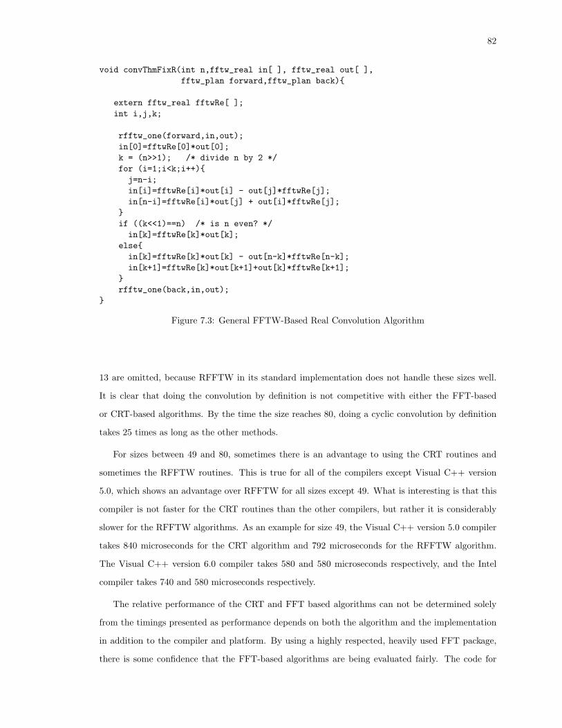
82
void convThmFixR(int n,fftw_real in[ ], fftw_real out[ ],fftw_plan forward,fftw_plan back){
extern fftw_real fftwRe[ ];int i,j,k;
rfftw_one(forward,in,out);in[0]=fftwRe[0]*out[0];k = (n>>1); /* divide n by 2 */for (i=1;i<k;i++){j=n-i;in[i]=fftwRe[i]*out[i] - out[j]*fftwRe[j];in[n-i]=fftwRe[i]*out[j] + out[i]*fftwRe[j];
}if ((k<<1)==n) /* is n even? */in[k]=fftwRe[k]*out[k];
else{in[k]=fftwRe[k]*out[k] - out[n-k]*fftwRe[n-k];in[k+1]=fftwRe[k]*out[k+1]+out[k]*fftwRe[k+1];
}rfftw_one(back,in,out);
}
Figure 7.3: General FFTW-Based Real Convolution Algorithm
13 are omitted, because RFFTW in its standard implementation does not handle these sizes well.
It is clear that doing the convolution by definition is not competitive with either the FFT-based
or CRT-based algorithms. By the time the size reaches 80, doing a cyclic convolution by definition
takes 25 times as long as the other methods.
For sizes between 49 and 80, sometimes there is an advantage to using the CRT routines and
sometimes the RFFTW routines. This is true for all of the compilers except Visual C++ version
5.0, which shows an advantage over RFFTW for all sizes except 49. What is interesting is that this
compiler is not faster for the CRT routines than the other compilers, but rather it is considerably
slower for the RFFTW algorithms. As an example for size 49, the Visual C++ version 5.0 compiler
takes 840 microseconds for the CRT algorithm and 792 microseconds for the RFFTW algorithm.
The Visual C++ version 6.0 compiler takes 580 and 580 microseconds respectively, and the Intel
compiler takes 740 and 580 microseconds respectively.
The relative performance of the CRT and FFT based algorithms can not be determined solely
from the timings presented as performance depends on both the algorithm and the implementation
in addition to the compiler and platform. By using a highly respected, heavily used FFT package,
there is some confidence that the FFT-based algorithms are being evaluated fairly. The code for

83
void convThmFix18C(fftw_complex in[ ], fftw_complex out[ ],fftw_plan forward,fftw_plan back){
fftw_one(forward,in,out);
in[0].re=out[0].re*(500.611111111) - out[0].im*(561.388888889);in[0].im=out[0].re*(561.388888889) + out[0].im*(500.611111111);in[1].re=out[1].re*(12.133584683) - out[1].im*(21.099917859);in[1].im=out[1].re*(21.099917859) + out[1].im*(12.133584683);in[2].re=out[2].re*(94.407642270) - out[2].im*(98.666882853);in[2].im=out[2].re*(98.666882853) + out[2].im*(94.407642270);in[3].re=out[3].re*(15.616912620) - out[3].im*(67.430407227);in[3].im=out[3].re*(67.430407227) + out[3].im*(15.616912620);in[4].re=out[4].re*(166.180429911) - out[4].im*(94.068867535);in[4].im=out[4].re*(94.068867535) + out[4].im*(166.180429911);in[5].re=out[5].re*(27.332203970) - out[5].im*(35.943153890);in[5].im=out[5].re*(35.943153890) + out[5].im*(27.332203970);in[6].re=out[6].re*(-101.522748384) - out[6].im*(-43.024837279);in[6].im=out[6].re*( -43.024837279) + out[6].im*(-101.522748384);in[7].re=out[7].re*(-5.978670532) - out[7].im*(-52.084927646);in[7].im=out[7].re*( -52.084927646) + out[7].im*(-5.978670532);in[8].re=out[8].re*(33.594257383) - out[8].im*(50.905817130);in[8].im=out[8].re*(50.905817130) + out[8].im*(33.594257383);in[9].re=out[9].re*(-51.722222222) - out[9].im*(104.055555556);in[9].im=out[9].re*(104.055555556) + out[9].im*(-51.722222222);in[10].re=out[10].re*(136.897432014) - out[10].im*(-48.880243019);in[10].im=out[10].re*(-48.880243019) + out[10].im*(136.897432014);in[11].re=out[11].re*(30.489963483) - out[11].im*(-14.168473458);in[11].im=out[11].re*(-14.168473458) + out[11].im*(30.489963483);in[12].re=out[12].re*(-42.921696061) - out[12].im*(104.969281723);in[12].im=out[12].re*(104.969281723) + out[12].im*(-42.921696061);in[13].re=out[13].re*(20.118703643) - out[13].im*(39.708730346);in[13].im=out[13].re*(39.708730346) + out[13].im*(20.118703643);in[14].re=out[14].re*(-149.300477352) - out[14].im*(-87.910528324);in[14].im=out[14].re*(-87.910528324) + out[14].im*(-149.300477352);in[15].re=out[15].re*(-8.728023731) - out[15].im*(24.514037217);in[15].im=out[15].re*(24.514037217) + out[15].im*(-8.728023731);in[16].re=out[16].re*(-80.445950891) - out[16].im*(-40.684129508);in[16].im=out[16].re*(-40.684129508) + out[16].im*(-80.445950891);in[17].re=out[17].re*(17.237548087) - out[17].im*(6.001599010);in[17].im=out[17].re*(6.001599010) + out[17].im*(17.237548087);
fftw_one(back,in,out);}
Figure 7.4: Example of an FFTW-Based Complex Convolution Algorithm

84
void generalConvThmFixedVec(int n,fftw_plan forward,fftw_plan back,fftw_complex in[],fftw_complex out[]){
int i;extern fftw_complex work[ ]; extern fftw_complex fixedVec[ ];
fftw_one(forward,in,out);for (i=0;i<n;i++){
work[i].re= (out[i].re*fixedVec[i].re - out[i].im*fixedVec[i].im);work[i].im= (out[i].re*fixedVec[i].im + out[i].im*fixedVec[i].re); }
fftw_one(back,work,out);}
Figure 7.5: General FFTW-Based Complex Convolution Algorithm
the CRT-based algorithms depends on the efficiency of the code produced by the SPL compiler.
Several deficiencies have been found in the SPL compiler that affects the performance of the CRT-
based algorithms. In section 7.2.2 several optimizations are presented that dramatically improve the
performance of the code produced by the SPL compiler for these algorithms. These optimizations
extend the window where CRT-based algorithms outperform FFT-based algorithms.
In order to motivate the optimizations discussed in section 7.2.2, it is worth taking a moment to
try to understand why the CRT algorithms are slower for certain points. In particular, Figure 7.7
shows especially poor performance for the improved split-nesting algorithm relative to RFFTW-
based convolutions for size 49, 65, and 77. Recall from chapter 6 however that the improved split-
nesting algorithm used fewer operations than the FFT-based convolution theorem for these points.
Figure 7.8 shows this same result in another way. Here, the number of operations for computing a
given size convolution via the improved split-nesting algorithm are normalized against the number of
operations required for computing the same size convolution via the FFT and convolution theorem.
In this way, it is seen that the improved split-nesting algorithm for sizes 49, 65 and 77 only require
about 60-80% as many operations as the FFT-based algorithms of the same sizes. It is somewhat
surprising therefore that the improved split-nesting algorithm performs badly relative to RFFTW
for these sizes.
Notice however, that the run-time performance for sizes near 77 are considerably better relative
to RFFTW than for 77 itself (see Figure 7.7). A look back to Table 6.5 from chapter 6 shows that
the operation counts show this as well (size 76 improved split-nesting requires 2348 operations, size
77 requires 3161 operations, and size 78 requires 2122 operations. Since the lines of straight-line
code used in these algorithms is proportional to the number of operations required, perhaps code

85
0.01
0.1
1
10
100
1000
2 5 8 11 14 18 22 26 30 35 40 45 50 55 63 66 75 80
Convolution Size
Mic
rose
cond
s
By Definition
Imp. Split-Nesting
RFFTW Based
(Intel C++ compiler v.6.0 on 800 mhz Pentium III)
Figure 7.6: Comparison of Convolution Algorithms on Real Inputs
length has something to do with the poor performance for sizes 49, 65, and 77.
To test this latter hypothesis another plot was made, plotting time per line of C code versus
number of lines of C code for each size convolution. This plot is shown in Figure 7.9. In this case the
x-axis represents the lines of code for a convolution; thus the convolutions are out of order in cases
where a larger convolution algorithm uses fewer lines of code (has fewer operations). For example,
convolutions of size 78, and 80 are to the left of size 77. This figure shows that the hypothesis is
correct, that is, performance degrades with the length of the code. In particular, notice that for
subroutines that are between 100 and 1200 lines, the run-time averages 0.0025 microseconds per line
of code, but as soon as the subroutine reaches 1400 lines, the average run-time cost nearly doubles.
Put another way, it is not just that certain size CRT algorithms are slower than their FFT
counterparts. It is that some CRT algorithms exceed the threshold of 1400 lines and the run-time
cost is prohibitive. In particular, while Figure 7.7 shows that some CRT algorithms exceeding size 48
are faster than RFFTW and some are slower, it turns out that CRT algorithms that are shorter than
1400 lines are always faster than their RFFTW counterparts and all (except one) CRT algorithms
that are longer than 1400 lines are slower than their RFFTW counterparts. Specifically, CRT
algorithms with fewer than 1400 lines are on average 52% faster than RFFTW-based convolutions
of the same size, while those over 1400 lines are 28% slower than the RFFTW-based convolutions
on average.

86
0
0.5
1
1.5
2
2 5 8 11 14 18 22 26 30 35 40 45 50 55 63 66 75 80
Ru
n T
ime
/ RF
FT
W R
un
Tim
e
RFFTW Based
ISN Intel
ISN VC6
ISN VC5
Figure 7.7: Improved Split-Nesting (ISN) versus RFFTW Convolution for 3 Compilers
0
0.2
0.4
0.6
0.8
1
1.2
2 5 8 11 14 18 21 24 27 32 35 39 44 48 51 55 60 65 69 75 78
Improved Split-NestingConvolution Theorem
Sizes 49, 65, and 77
Figure 7.8: Improved Split-Nesting (ISN) Operations Divided by Convolution Theorem Operations

87
0
0.001
0.002
0.003
0.004
0.005
0.006
102
186
222
300
466
516
569
822
983
1154
1258
1522
1829
1955
2336
3285
4501
4991
6427
Lines of C code
Ave
rage
Tim
e in
Mic
rose
con
ds
Per
Lin
e of
Cod
e
Figure 7.9: Average Run Time Per Line of Code for Various Size Convolution Algorithms
Exploration of Performance Decline for Long Code Sequences
It was shown in Figure 7.9 that as subroutines start to exceed 1400 lines, the run-time performance
begins to suffer. The question then becomes is this a hardware issue or a software or compiler issue?
A number of experiments were run to try to determine the cause of the performance degradation.
The first test was to split the large convolution subroutines into a series of smaller subroutines. Thus
if it was the case that the compiler stopped optimizing as subroutines became too large, this should
solve the problem. It turns out that breaking the convolution into smaller subroutines exacerbates
the problem, indicating that it was probably not a compiler problem. The fact that three different
compilers (Intel C++ version 6.0, MS Visual C++ 6.0 and Visual C++ 5.0) all exhibit the same
behavior is further evidence that the problem is not due to the compilers.
A more likely culprit is that the size of the code is causing cache misses for the very long code
sequences. To test this, a short convolution with very good performance was timed for 100,000
iterations and the performance recorded. Next, this same convolution was timed, but in between
each iteration a large time consuming subroutine was called that would fill up the cache. The new
time for the 100,000 iterations of the small convolution algorithm could be obtained by subtracting
the time taken for the 100,000 iterations of the large time consuming subroutine. The code for this

88
experiment is shown here.
start = clock();srand(RANDSEED); /* seed random number generator */for (i = 0; i<ITER; i++){ /* do 100,000 iterations */
for (j=0; j < n; j++){in[j] = ((double) (rand() % 10000));
}splitNesting20(out,in); /* convolution of fixed vector with vector
in[]; answer is stored in out[] */largeTimeConsumingRoutine(in);
}finish = clock(); elapsed_time1 = ((double)(finish-start));
srand(RANDSEED);start = clock();for (i = 0; i<ITER; i++){
for (j=0; j < n; j++){in[j] = ((double) (rand() % 10000));
}largeTimeConsumingRoutine(in);
}finish = clock();
elapsed_time2 = ((double)(finish - start));elapsed_time1 = elapsed_time1-elapsed_time2;
This test, which was repeated for several examples, showed the 40% to 50% performance decline
that was expected. This suggests that using loops for larger algorithms to keep code size under
1400 lines will yield a 40% to 50% performance gain for the machine used in this experiment (800
mhz Pentium III). This also suggests that newer computers with larger caches will likely outperform
FFT-based convolutions for a larger window than was shown in Figure 7.7. Finally, it shows that
building custom hardware whose performance per line of code does not degrade, it would be possible
to realize the advantage for CRT-based algorithms over FFT-based algorithms for the entire window.
Note that a custom hardware solution is not far-fetched given that signal processing boards that
incorporate convolutions currently exist.
Since a 40% to 50% performance gain can be realized just by keeping the code length under
1400 lines, optimizations that involve trading straight-line code to looped code will be explored in
section 7.2.2 below.
7.2.2 Basic Optimizations for SPL Generated CRT Algorithms
The SPL compiler developed as part of the SPIRAL project [24] was primarily designed to
generate straight line code for FFT algorithms. Its use in generating CRT algorithms has therefore
uncovered a number of weaknesses that can be easily fixed in its next generation. First, since the

89
CRT algorithms get complicated as they get longer, the straight line code becomes excessive, which
can slow down the algorithm by 40% to 50% or more due to cache misses. For example, the single
worst performing convolution in Figure 7.7 is for size 77; it contains 3158 lines of C code, and takes
85% longer than an RFFTW-based convolution. Thus for large sizes, changing to looped code is
critical.
However, as previously mentioned, the SPL compiler is not necessarily tuned for creating loop
code. First, the SPL compiler puts in a number of unnecessary loops that do nothing but copy one
array to another, when the first array is never subsequently used and need not be protected. This is
equivalent to an identity matrix composition; these are automatically removed by the SPL compiler
in the straight-line code, but not the looped code. Second, the SPL compiler does not loop diagonal
matrices. Since the CRT algorithms contain a very large diagonal matrix, many lines of code can be
saved by storing this diagonal in an array and computing the Hadamard Multiplications with a loop.
Finally, non-stride permutation matrices are never implemented via loops by the SPL compiler. By
passing in an array of pointers, permutations can be implemented in a loop, considerably reducing
code size and run-time.
These optimizations can be easily implemented in a next generation compiler but for now they
have to be done by hand; this is both tedious and very time consuming, so it is only done for three
particularly bad performing sizes in order to illustrate the potential gain in performance. Figure 7.10
shows the effect of these basic optimizations for convolutions of size 49, 65, and 77 on the Intel
Compiler (results are similar for the other compilers). Moving from straight-line code to loops
adds an initial disadvantage, but after changing the diagonal to looped code, removing identities
and changing the permutations to looped code (note that size 49 contains no permutations), the
disadvantage is removed, and ultimately the run time is 10% to 30% faster than RFFTW-based
convolutions of the same size.
It is quite likely that the algorithms can be further improved. Looping can be more finely
controlled but was not. The looped code in these examples used loops for any matrix blocks of size
60 or more, but other block sizes may lead to better times, or selectively turning looping on and
off could lead to further improved times. Further, it is not clear whether the best CRT algorithms
are being used. To find the limit of these algorithms a search project on the order of the SPIRAL
project (see [24]) is needed to ultimately find the limit of the window. Still, it is clear that the
window where these algorithms are competitive with RFFTW extends beyond 80 and probably well
beyond 100. However, as will be shown in section 7.3, the existence of a window regardless of the
size, can be used to improve the performance of larger convolutions.

90
0%
50%
100%
150%
200%
250%
49 65 77Convolution Size
Run
Tim
e as
a P
erce
nt o
f R
FF
TW
Run
Tim
e
ISN Straight LineISN Loop Block size 60ISN Loop 60; Loop DiagonalISN Loop 60; Loop Diagonal; Remove unnecessary IdentitiesISN Loop 60; Loop Diagonal; Remove Identities; Loop Permutations
Figure 7.10: Effect of Basic Optimizations on Run-Time for 3 CRT Convolutions
7.2.3 Is Improved Split-Nesting the Best Choice?
The timings discussed thus far compare convolution algorithms created via the convolution theorem
using RFFTW and CRT-based algorithms using the improved split-nesting algorithm. However, as
was discussed in chapters 3 and 6, there are hundreds of different ways of constructing CRT-based
algorithms of various sizes and some of these may lead to faster implementations than the improved
split-nesting algorithm. However, without a significant search project, and a next generation SPL
compiler, this cannot be fully explored.
Figure 7.11 does gives a justification for using the improved split-nesting algorithm as a general
purpose algorithm. For size 33 (and others) it performs better than implementations of other split-
nesting algorithms, Agarwal-Cooley algorithms (While there are dozens of ways of constructing
Agarwal-Cooley and split-nesting algorithms of size 33, two obvious choices for each method were
picked for comparison purposes.) as well as the basic CRT algorithm and Winograd algorithm.
However, these times are based on straight-line code directly from the SPL compiler. It is possible
that with looping and the optimizations discussed in section 7.2.2 that the improved split-nesting
algorithm might perform worse in some cases than the other choices under optimal conditions.
Furthermore, the implementation of the improved split-nesting algorithm used here is based on a

91
0
1
2
3
4
5
6
ImprovedSplit Nest
CRT SplitNest(A)
Ag-Cooley(A)
SplitNest(B)
Ag-Cooley(B)
RFFTW Winograd
Mic
rose
con
ds
Figure 7.11: Run-Time for Various Size 33 CRT-Based Convolutions and RFFTW
version that minimizes operation counts; there are several additional ways to construct the algorithm
that may improve run-time.
Although the ultimate goal of this work is not to find the best CRT convolution algorithm, but
rather to show that there is a significant window where these algorithms are viable, it is important
to show that the algorithms used for timing purposes are reasonable choices. While determining
the best CRT-based implementation is beyond the scope of this thesis, Figure 7.11 shows that the
improved split-nesting algorithm, that minimizes operation counts, is a reasonable implementation
choice. The best implementation depends on the compilers and platforms used and requires a
significant engineering approach along the lines of the SPIRAL project [24] to carry out.
Figure 7.11 shows that there is a difference in performance depending on how the algorithms are
combined. There is a 10% difference in performance between the two versions of Agarwal-Cooley
and the variants of the split-nesting algorithm. The only difference in these variants is the order of
various tensor products. Since the tensor products involve rectangular matrices, the wrong order
can lead to a blow-up in row dimension, and a significant performance penalty.
One final item to note is that the Winograd algorithm is more than 2.5 times slower than the
improved split-nesting algorithm for this size. Winograd’s algorithm trades multiplications for a
large increase in additions, and in modern architectures this is a bad trade. The CRT algorithm,
which uses Winograd’s idea, but substitutes more sensible linear convolutions as the building blocks
is much more competitive.
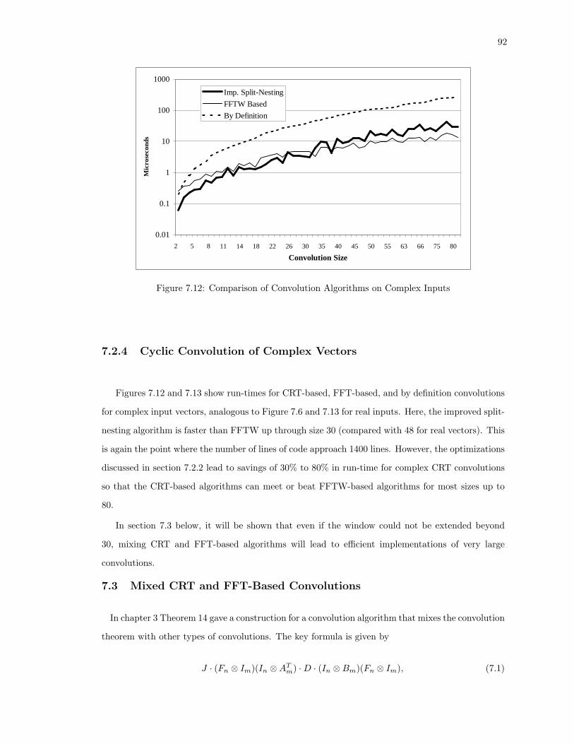
92
0.01
0.1
1
10
100
1000
2 5 8 11 14 18 22 26 30 35 40 45 50 55 63 66 75 80
Convolution Size
Mic
rose
cond
s
Imp. Split-Nesting
FFTW Based
By Definition
Figure 7.12: Comparison of Convolution Algorithms on Complex Inputs
7.2.4 Cyclic Convolution of Complex Vectors
Figures 7.12 and 7.13 show run-times for CRT-based, FFT-based, and by definition convolutions
for complex input vectors, analogous to Figure 7.6 and 7.13 for real inputs. Here, the improved split-
nesting algorithm is faster than FFTW up through size 30 (compared with 48 for real vectors). This
is again the point where the number of lines of code approach 1400 lines. However, the optimizations
discussed in section 7.2.2 lead to savings of 30% to 80% in run-time for complex CRT convolutions
so that the CRT-based algorithms can meet or beat FFTW-based algorithms for most sizes up to
80.
In section 7.3 below, it will be shown that even if the window could not be extended beyond
30, mixing CRT and FFT-based algorithms will lead to efficient implementations of very large
convolutions.
7.3 Mixed CRT and FFT-Based Convolutions
In chapter 3 Theorem 14 gave a construction for a convolution algorithm that mixes the convolution
theorem with other types of convolutions. The key formula is given by
J · (Fn ⊗ Im)(In ⊗ATm) ·D · (In ⊗Bm)(Fn ⊗ Im), (7.1)

93
0
0.5
1
1.5
2
2.5
3
2 5 8 11 14 18 22 26 30 35 40 45 50 55 63 66 75 80
Convolution Size
Run
Tim
e / F
FTW
Run
Tim
e
ISN Intel
ISN VC 6
FFTW Based
ISN VC 5
Figure 7.13: Improved Split-Nesting (ISN) versus FFTW Convolution for 3 Compilers
where D is a well defined diagonal matrix and J is the anti-identity matrix. The implication is that
since there is a window where the CRT algorithms are faster than the FFT-based algorithms, large
convolutions of size mn where m is chosen to be within the window and n is chosen outside of the
window, should be faster than convolutions that use pure FFT methods or pure CRT methods. This
was confirmed for operation count in chapter 5 and will be confirmed for run-time below.
Figure 7.14 contains C code for computing a size 3m cyclic convolution that mixes a size three
CRT algorithm with a size m FFT using (7.1). The code was created by generating C code for the
size three CRT algorithm (essentially AT ·D · B), and then adding a size m loop and two Fourier
transforms. The looped code for composing the diagonal matrix was also added, because the SPL
compiler currently uses straight line code for diagonal composition. The final modification involves
doubling up some lines so that the listing fits on a single page.
The C code in Figure 7.14 will generate a size 3m cyclic convolution and return the answer
in reverse order, (note the order can easily be fixed by adding a three line loop at the end). A
precomputed vector is passed into the subroutine in the array diagVec[], as well as a size m plan
for FFTW.
FFTW uses a plan in order to create machine adaptable optimization (see [10]). The specific
call to fftw in the listing contains several parameters besides the input and output arrays. The
additional parameters tell FFTW to generate three FFTs and that the input and output arrays

94
/*! +------------------------------------------------------------+! | Generated by SPL Compiler 3.29 |! +------------------------------------------------------------+! Command-line options: -O -B 2*/void mix3xFm(double y[],double x[],int m,double diagVec[],
fftw_plan forward){int i0,i1;double f0,f1,f2,f3,f4,...,f23;static double t1[10],t2[3*4096*2],t3[10],t4[3*4096*2];
fftw(forward,3,((fftw_complex*)x),3,1,((fftw_complex*)t4),3,1);
for (i0=0; i0<m; i0++) {f0=t4[6*i0+2] + t4[6*i0+4]; f1=t4[6*i0+3] + t4[6*i0+5];f2=t4[6*i0+4] - t4[6*i0+2]; f3=t4[6*i0+5] - t4[6*i0+3];t3[2]=t4[6*i0] + f0; t3[3]=t4[6*i0+1] + f1;t3[0]=t4[6*i0]; t3[1]=t4[6*i0+1];t3[4]=t4[6*i0] + f2; t3[5]=t4[6*i0+1] + f3;f4=t3[2] + f2; f5=t3[3] + f3;f6=f4 + f0; f7=f5 + f1;t3[6]=f6 + f0; t3[7]=f7 + f1;t3[8]=t4[6*i0+4]; t3[9]=t4[6*i0+5];
for (i1=0;i1<5;i1++){f8=diagVec[i0*10+2*i1] * t3[2*i1];f9=diagVec[i0*10+2*i1+1] * t3[2*i1+1];f10=diagVec[i0*10+2*i1] * t3[2*i1+1];f11=diagVec[i0*10+2*i1+1] * t3[2*i1];t1[2*i1]=f8 - f9; t1[2*i1+1]=f10 + f11;
}
f12=t1[0] + t1[4]; f13=t1[1] + t1[5];f14=t1[2] + t1[6]; f15=t1[3] + t1[7];f16=t1[4] + t1[6]; f17=t1[5] + t1[7];t2[6*i0]=f12 + f14; t2[6*i0+1]=f13 + f15;f18=f14 + t1[6]; f19=f15 + t1[7];f20=f18 + t1[6]; f21=f19 + t1[7];t2[6*i0+2]=f20 - f16; t2[6*i0+3]=f21 - f17;f22=f20 + f16; f23=f21 + f17;t2[6*i0+4]=f22 + t1[8]; t2[6*i0+5]=f23 + t1[9];
}
fftw(forward,3,((fftw_complex*)t2),3,1,((fftw_complex*)y),3,1);}
Figure 7.14: Listing for Size 3m Mixed Algorithm

95
should be read and written at stride three. By allowing the user to specify strides, FFTW makes it
easy to generate a call that is equivalent to (Fm ⊗ I3).
Table 7.1 shows the timing results of mix3xFm from the listing in Figure 7.14 versus convolutions
computed with FFTW alone. The mixed algorithm is 12% faster for size 192, and 9% faster for size
384, but roughly even for sizes 384, and 768, and actually slower for sizes 3072 and 6074. It is not clear
why the advantage vanishes, however, it is likely that FFTW found a more efficient way of computing
F3072 that does not directly compute F512. An FFT of size 3072 can be computed in different ways, by
using different parameters in the factorization in (2.7). For example, (F6⊗I512)T 3072512 (I6⊗F512)L3072
6 ,
(F2 ⊗ I1536)T 30721536 (I2 ⊗ F1536)L3072
2 , or in hundreds of other ways. The code for mix3xFm severely
limits the number of ways of factoring 3072. However, it should be noted that mix3xFm is not the
only way to mix a size 3 CRT with a size 1072 Fourier transform. By better integrating the CRT
code with FFTW’s planning mechanism, or by searching for an optimal solution among various
factorizations, there is no reason why the mixed algorithm should not be faster for any size. This is
formalized in section 7.3.1.
Table 7.2 shows the timing results of a similar mixed algorithm that combines a size 5 CRT-based
algorithm with any size Fourier transform. In this table there is a 4% to 9% advantage for each of
the samples tested.
Table 7.3 shows timing results for a mixed algorithm that combines a size 15 CRT algorithm
(created via the Agarwal-Cooley algorithm on the size 3 and 5 CRT algorithms) with any size
Fourier transform. For sizes 480 and 1920 there is no advantage, but for sizes 7680 and 15360 a
speed advantage of about 25% can be realized.
Table 7.1: Run-Time for FFTW-Based Convolutions versus Mixed Convolutions of Size 3m
N FFTW Mix Advantage192=3x64 27 24 12%384=3x128 66 60 9%768=3x256 141 139 1%1536=3x512 353 340 3%3072=3x1024 994 1235 -24%6144=3x2048 3419 4431 -30%

96
Table 7.2: Run-Time for FFTW-Based Convolutions versus Mixed Convolutions of Size 5m
N FFTW Mix Advantage320=5x64 51 47 9%640=5x128 119 114 4%1280=5x256 267 248 7%2560=5x512 634 599 6%5120=5x1024 2660 2483 7%10240=5x2048 7610 7241 5%
Table 7.3: Run-Time for FFTW-Based Convolutions versus Mixed Convolutions of Size 15m
N FFTW Mix Advantage480=15x32 89 94 -5%960=15x64 196 171 13%1920=15x128 430 437 -2%3840=15x256 1482 1288 13%7680=15x512 5054 3861 24%15360=15x1024 13195 9738 26%
7.3.1 Generalizing Mixed Algorithm Timing Results
It is clear that by combining CRT-based algorithms within a specified window with FFT algorithms
outside of the window an advantage could sometimes be realized versus computing the convolution
via an FFT alone. In this section, it is shown that this is the rule and not the exception, and that
the cases where the method does not work are really problems of optimization, that can be overcome
by better integrating the algorithms with FFTW’s planning mechanism. The following notation will
be used to formalize the result.
Notation 3 Let t(a) represent the time in microseconds it takes to execute the algorithm a.
Let U1 be a CRT-based convolution algorithm of size N and let U2 be an FFT-based convolution
algorithm of size N , so that
U1 = JNAT1 D1B1
U2 = JNFND2FN ,
with,
D1 = CT1 JNv1
D2 = F−1N JNv2.
97
Further suppose that t(JN ) = k, and that N is within the window so that t(U1) = n + k
microseconds total and t(U2) = n+k + c, with c > 0. Now let W1 be a mixed algorithm of size MN
and let W2 be an FFT-based algorithm of size MN .
W1 = JMN (FM ⊗ IN )(IM ⊗AT1 )D′
1(IM ⊗B1) · (FM ⊗ IN )
W2 = JMNFMND′2FMN
= (FM ⊗ IN )TMNN (IM ⊗ FN )D′
2 · (IM ⊗ FN )TMNN (FM ⊗ IN ).
Now, observe that t(D′1) = M · t(D1) and t(D′
2) = M · t(D2) since the time taken to apply a
square diagonal to a vector is proportional to the number of rows of the diagonal. Also, t(JMN ) =
M ·t(JN ) = Mk. This assumes that repeated calls in a larger algorithm behave the same as repeated
calls in isolation, which is a reasonable assumption, but may not be true for machines and cache
sizes. Thus
t(W1) = Mk + N · t(FM ) + M(t(U1)− t(JN )) + N · t(FM )= Mk + 2N · t(FM ) + Mn,
t(W2) = Mk + N · t(FM ) + t(TMNN ) + M(t(U2)− t(JN )) + t(TMN
N ) + N · t(FM )= Mk + 2N · t(FM ) + 2t(TMN
N ) + M(n + c).
It follows that t(W2) = t(W1) + 2t(TMNN ) + Mc where the 2t(TMN
N ) can be 0 if gcd(M, N) = 1.
So that the initial advantage increases with the size of M .
A similar argument substituting operation count for timing, was shown in chapter 6.
The implication is that the reason the advantage was not always realized in Tables 7.1, 7.2, and
7.3, is the static mixed algorithm interfered with FFTW’s ability to choose the best factoring for its
FFTs, or less likely, there was a cache issue. Thus by better integrating the mixed algorithm with
FFTW’s planning mechanism faster convolution algorithms should be attainable.

98
Chapter 8: Conclusions
The use of CRT-based convolution algorithms was suggested 25 years ago by S. Winograd in an
investigation of the complexity of convolution and related problems [29, 30]. In spite of numerous
developments since that time by Agarwal and Cooley, [1], Selesnick and Burrus [22], and others
[19, 27], there has not been a definitive study that investigates the practical feasibility of CRT-
based convolution algorithms and compares them to FFT-based approaches. The net result is that
despite all of the development, the majority of convolution algorithms are computed via the FFT
and convolution theorem except in the case of very small convolutions.
The original justification for the Winograd algorithms is the reduction in multiplications; how-
ever, in many modern architectures, the cost of additions and multiplications are roughly the same.
Consequently it is more important to focus on the total number of operations. Moreover, memory
accesses and cache considerations can be even more important than the number of arithmetic opera-
tions. Ultimately the goal is to provide an infrastructure to investigate the relative costs of different
algorithms using various cost functions.
The goal of this thesis was to determine whether CRT-based algorithms are of practical value
on current architectures, and to provide an infrastructure and approach for answering this question
as architectures evolve. The results show that not only are the algorithms viable for small sized
convolutions, but in fact they can be combined with FFT algorithms to create very large convolution
algorithms that are faster than pure FFT-based methods as well as pure CRT-based methods.
Highlights of the research contributions are outlined below.
• Existing algorithms from the literature were put into a common framework of bilinear algo-
rithms, and it was shown that the various techniques developed over the years can all be
shown to be generated via tensor products, direct sums, and the Chinese Remainder Theo-
rem. This common framework allows for easy comparison, analysis, and implementation of
the algorithms, and also allows for the creation of an “algebra of algorithms,” which can be
manipulated, combined, generated in a structured and automated way. This was not merely
a matter of notation or style, but was a crucial foundation for systematically studying convo-
lution algorithms in the project.
• An extensive search was performed to find the algorithm with fewest operations. This search
led to the discovery of a new algorithm “improved split-nesting” that uses fewer operations

99
than previously published algorithms.
• A method of combining CRT-based and FFT-based algorithms was introduced and shown to
outperform (in both operation count and run-time) pure CRT-based and FFT-based convolu-
tions for certain large size convolutions.
• An infrastructure for experimenting, manipulating, and automatically generating convolution
algorithms was also developed, which was crucial for generating a test of this magnitude. In
particular, the testing procedure greatly exceeded any previous work, and would have been
simply impossible to do by hand. For example, a size 77 complex cyclic convolution contains
more than 25,000 lines of C code, while the entire tested set of sizes between 2 and 80 contains
more than 319,000 lines of straight-line code and more than 196,000 lines of looped code. The
timing process discussed in chapter 7 involved generating and compiling more than 10 million
lines of C code. Doing such a project without an infrastructure, would be simply impossible.
The thesis research has thus achieved its stated goal of determining whether these algorithms are
viable. In fact, the algorithms are not only viable, but they could be a significant tool for anyone
that needs efficient implementations of convolution algorithms. The project also opened several
avenues for future research.
Future research can proceed in several directions. First, several improvements for the SPL
compiler were outlined in chapter 7. Some of these are already being implemented, and may lead to
an expansion of the window where CRT-based convolutions are faster than FFT-based convolutions.
Second, search methods should be used to find the best implementation (not just minimal operation
count) so that nearly optimal implementations can be obtained for a given computer. The search
methods should include various combinations of the CRT-algorithms with FFT algorithms. This
work is being undertaken as part of the SPIRAL project [24]. Third, it would be interesting to use
other cost functions, such as memory accesses and cache misses, when comparing the algorithms in
this thesis. Finally, it would be worthwhile to try to extend the techniques in this thesis to other
problems in signal and image processing and other application areas where there is a rich space of
algorithms with mathematical structures.

100
Bibliography
[1] R. C. Agarwal and J. W. Cooley. New algorithms for digital convolution. IEEE Trans. Acoust.Speech and Signal Proc., 25:392–410, 1977.
[2] L. Auslander, J.R. Johnson, and R.W. Johnson. Automatic implementation of fft algorithms.Technical Report DU-MCS-96-01, Drexel University, July 1996.
[3] G. D. Bergland. A fast fourier transform for real-valued series. Communications of the ACM,11:703–710, 1968.
[4] R. E. Blahut. Algebraic Methods for Signal Processing and Communications Coding. Springer-Verlag, New York, 1992.
[5] C. S. Burrus and P. W. Eschenbacher. An in-place, in-order prime factor FFT algorithm. IEEETrans. Acoust., Speech, Signal Processing, ASSP-29(4):806–817, August 1981.
[6] C.S. Burrus and T.W. Parks. DFT/FFT and Convolution Algorithms: Theory and Implemen-tation. John Wiley and Sons, New York, NY, USA, 1985.
[7] S. A. Cook. Thesis:On the minimum computation time of functions. Harvard Thesis, 1966.
[8] J. W. Cooley. Automated generation of optimized convolution algorithms. In D. V. Chudnovskyand R. D. Jenks, editors, Computer Algebra, Lecture Notes in Pure and Applied Mathematics.Marcel Dekker, Inc., New York and Basel, 1989.
[9] J. W. Cooley and J. W. Tukey. An algorithm for the machine calculation of complex fourierseries. Math. Comp., 19:297–301, 1965.
[10] M. Frigo and S. Johnson. FFTW: An adaptive software architecture for the FFT. Proceedings ofthe IEEE International Conference on Acoustics, Speech, and Signal Processing, 3:1381–1384,1998.
[11] I. J. Good. The interaction algorithm and practical fourier analysis. J. Royal Statist. Soc.,B20:361–375, 1958.
[12] R. A. Horn and C. R. Johnson. Topics in Matrix Analysis. Cambridge University Press,Cambridge, 1991.
[13] J. R. Johnson, R. W. Johnson, D. Rodriguez, and R. Tolimieri. A methodology for designing,modifying and implementing fourier transform algorithms on various architectures. CircuitsSystems Signal Process, 9(4):449–500, 1990.
[14] R. W. Johnson, C.-H. Huang, and J. R. Johnson. Multilinear algebra and parallel programming.Journal of Supercomputing, 5:189–218, 1991.
[15] D. E. Knuth. Seminumerical Algorithms - The Art of Computer Programming Volume 2.Addison-Wesley, Reading, Massachusetts, 2nd. edition, 1981.
[16] S. Lang. Algebra. Addison-Wesley, Redwood City, CA, 1984.
[17] C. Van Loan. Computational Frameworks for the Fast Fourier Transform. Society for Industrialand Applied Mathematics, Philadelphia, PA, 1992.
[18] M. B. Monagan, editor. Maple V Programming Guide (Version A): Release 5. Springer-Verlag,New York, 1998.

101
[19] H. J. Nussbaumer. Fast Fourier Transform and Convolutional Algorithms. Springer-Verlag,New York, 2nd. edition, 1982.
[20] W. H. Press, S.A. Teukolsky, W.T. Vetterling, and B.P. Flannery. Numerical Recipes in C -The Art of Scientific Computing, 2nd ed. Cambridge University Press, 1992.
[21] C. M. Rader. Discrete fourier transform when the number of data samples is prime. Proc.IEEE, 56(6):1107–1108, 1968.
[22] I. Selesnick and C. Burrus. Automatic generation of prime length FFT programs. IEEETransactions on Signal Processing, 44:14–24, 1996.
[23] H. V. Sorensen, D. L. Jones, M. T. Heidman, and C. S. Burrus. Real-valued fast fouriertransform algorithms. IEEE Transactions on Acoustics, Speech, and Signal Processing, 35:849–863, 1987.
[24] SPIRAL. Spiral-signal processing algorithms implementation research for adaptable libraries,2000. http://www.ece.cmu.edu/∼spiral.
[25] C. Temperton. Implementation of a self-sorting in-place prime factor FFT algorithm. J. Com-put. Phys., 58:283–299, 1985.
[26] L. H. Thomas. Using a computer to solve problems in physics. In Applications of DigitalComputers. Ginn and Co., 1963.
[27] R. Tolimieri, M. An, and C. Lu. Algorithms for Discrete Fourier Transform and Convolution.Springer-Verlag, New York, NY, 1997.
[28] A. L. Toom. Soviet Mathematics, 3:714–716, 1963.
[29] S. Winograd. Some bilinear forms whose multiplicative complexity depends on the field ofconstants. Math. Syst. Theor., 10:169–180, 1977.
[30] S. Winograd. Arithmetic Complexity of Computations. CBMS-NSF Regional Conf. Ser. Appl.Math. Society for Industrial and Applied Mathematics, Philadelphia, PA, 1980.
[31] J. Xiong, J. Johnson, R. Johnson, and D. Padua. SPL: A Language and Compiler for DSPAlgorithms. In Proc. PLDI, pages 298–308, 2001.

102
Vita
Anthony Breitzman Sr. was born in New Jersey in November of 1966. Since 1993, he has worked
for CHI Research, Inc., a consulting firm that analyzes patents and other publicly available data
to track the technological developments of government, university, and commercial laboratories, in
order to identify opportunities and competitive advantages for its clients. In 1996 Anthony became
the youngest vice president in the firm’s 30 year history.
Anthony is considered an expert in constructing quantitative evaluations of companies’ techno-
logical strengths and weaknesses, and has been invited to the national meetings of the World Future
Society, the American Chemical Society, and the Society of Competitive Intelligence Professionals,
amongst others, to speak on topics such as using patent analysis to assess competitor companies, us-
ing patent indicators to identify merger and acquisition targets, and using patent metrics to identify
attractive investment opportunities.
He is the primary inventor/author of a US patent for choosing stock portfolios based on technol-
ogy strengths. In addition he has 11 published articles (the four most recent are listed below) and
a book chapter.
Prior to joining CHI Research, Anthony was a graduate student at Temple University where
he studied mathematics and taught calculus, algebra, and finite math. He has a B.S. degree in
mathematics from Stockton State College (1989), an M.A. degree in Mathematics from Temple
(1992), and an M.S. degree in Computer Science from Drexel University (1998). He is a member of
Upsilon Pi Epsilon, the honor society of computer science and maintains a 4.0 grade point average
at Drexel.
Most Recent Publications:
1. “Automatic Derivation and Implementation of Fast Convolution Algorithms”, J.R. Johnsonand A. Breitzman, Forthcoming in Journal of Symbolic Computation.
2. “Using Patent Citation Analysis to Target/Value M&A Candidates,” A. Breitzman and P.Thomas, Research Technology Management, 45, 5, 28-36, September-October, 2002.
3. “The Many Applications of Patent Analysis,” A. Breitzman and M.E. Mogee, Journal ofInformation Science, 28, 3, 2002, pp. 187-205.
4. “Technological Powerhouse or Diluted Competence – Techniques for Assessing Mergers viaPatent Analysis,” A. Breitzman, P. Thomas and M. Cheney, R&D Management 4-19, January,2001.
