fast 3d modeling of borehole induction measurements in dipping … · fast 3d modeling of borehole...
TRANSCRIPT
Fast 3D Modeling of Borehole Induction Measurements in Dipping and
Anisotropic Formations using a Novel Approximation Technique
Guozhong Gao1, Carlos Torres-Verdín
1, and Sheng Fang
2
INTRODUCTION
Integral equations have been widely used to simulate
EM scattering in geophysical prospecting and antenna
design applications. A number of applications and develop-
ments of integral equations for the simulation of subsurface
geophysical problems have been reported, including 3D
EM scattering in the presence of complex geometrical
structures (Hohmann, 1975, and 1983, Wannamaker, 1983,
Xiong, 1992, Gao et al., 2002, Hursan et al., 2002, and Fang
et al., 2003, among others).
Solution of EM scattering by integral equations includes
two sequential steps. First, the spatial distribution of the
electric field within scatterers is computed via a discre-
tization scheme. Second, the internal scattering currents are
“propagated” to receiver locations. It is often necessary to
discretize the scatterers into a large number of cells depend-
ing on (a) frequency, (b) electrical conductivity contrast, (c)
size of the scatterers, and (d) proximity of the source and/or
the receiver to the scatterers. This discretization gives rise
to a full complex linear system of equations whose solution
yields the spatial distribution of the internal electric field.
July-August 2004 PETROPHYSICS 335
PETROPHYSICS, VOL. 45, NO. 4 (JULY-AUGUST 2004); P. 335–349; 18 FIGURES, 1 TABLE
ABSTRACT
Macroscopic electrical anisotropy of rock formations
can substantially impact estimates of fluid saturation per-
formed with borehole electromagnetic (EM) measure-
ments. Accurate and expedient numerical simulation of
the EM response of electrically anisotropic and dipping
rock formations remains an open challenge, especially in
the presence of borehole and invasion effects.
This paper introduces a novel efficient 3D EM approx-
imation based on a new integral equation formulation.
The main objective of this approximation is to simulate
the multi-component borehole EM response of electri-
cally anisotropic rock formations. Firstly, the internal
electrical field is expressed as the product of spatially
smooth and rough components. The rough component is a
scalar function of location, and is governed by the back-
ground electric field. A vectorial function of location is
used to describe the smooth component of the internal
electric field, here referred to as the polarization vector.
Secondly, an integral equation is constructed to describe
the polarization vector. Because of the smooth nature of
the polarization vector, relatively few unknowns are
needed to describe it, thereby making its solution
extremely efficient. One of the main features of the new
approximation is that it properly accounts for the coupling
of EM fields necessary to simulate the response of electri-
cally anisotropic rock formations.
Tests of accuracy and computer efficiency against 1D
and 3D finite-difference simulations of the EM response
of tri-axial induction tools show that the new approxima-
tion successfully competes with accurate finite-difference
formulations, and provides superior accuracy to that of
standard approximations. Numerical simulations involv-
ing more than 106 discretization cells require only several
minutes per frequency and instrument location when per-
formed on a Silicon Graphics workstation with a 300
MHz, IP30 processor.
Manuscript received by the Editor September 1, 2003; revised manuscript received April 26, 2004.1Dept. of Petroleum and Geostystems Eningineering, The University of Texas at Austin, Austin, TX USA.2Baker Atlas, Houston, TX USA.
©2004 Society of Petrophysicists and Well Log Analysts. All rights reserved.
Requirements of computer memory increase quadratically
with a linear increase in the number of discretization cells.
Moreover, the need to solve a large, full, and complex linear
system of equations places significant constraints on the
applicability of 3D integral equation methods.
There are several numerical strategies used to overcome
the difficulties associated with integral equation formula-
tions of EM scattering. Fang et al. (2003) recently reported
one such strategy. Their simulation approach makes
explicit use of the symmetry properties of Toeplitz matri-
ces. Fang et al.’s (2003) algorithm also applies a suitable
combination of BiCGSTAB(l) (Bi-Conjugate Gradient
STABlized (l)) (Sleijpen and Fokkema, 1993) and the FFT
(Fast Fourier Transform) to iteratively solve the linear sys-
tem of equations. The latter method is a natural extension of
the widely used CG-FFT (Conjugate Gradient-Fast Fourier
Transform) strategy (Catedra et al., 1995) to compute EM
fields. Despite these significant improvements, integral
equation methods are still impractical for routine use in the
interpretation of borehole EM data. An alternative
approach is to develop an approximate solution. Several
approximations to the integral equation formulation have
been proposed in the past. These include Born (1933),
Extended Born (Habashy et al., 1993 and Torres-Verdin and
Habashy, 1994), and Quasi-Linear (Zhdanov and Fang,
1996, and Zhdanov, 2002). However, none of the integral
equation approximations published to date has been formu-
lated to approach the simulation of 3D EM scattering in the
presence of electrically anisotropic media. Developing
such an approximation is the main thrust of this paper.
Very recently, a novel approximation technique was
introduced that has the ability to accurately and efficiently
model borehole EM scattering in the presence of
anisotropic rock formations (Gao et al., 2003). The present
paper describes further developments performed in the
implementation, testing, and benchmarking of Gao et al.’s
(2003) novel integral equation approximation. This approx-
imation attempts to synthesize the spatial variability of the
secondary electric currents within a scatterer in two man-
ners. First, a multiplicative term is introduced to “capture”
the spatial variability of the secondary electric currents due
to the close proximity of the EM source to the scatterer. A
second multiplicative term is used to synthesize spatial
variations in the phase and polarization of the secondary
electric currents due to spatial variations in electrical con-
ductivity, including those due to electrical anisotropy. It is
shown that for borehole logging applications the latter
multiplicative term is spatially smoother than the first term
and hence can be described with fewer discretization
blocks. Moreover, the accuracy of the proposed approxima-
tion depends on both the choice of the background model
and the spatial distribution and number of discretization
blocks.
This paper is organized as follows: First the integral
equation method is introduced together with the theory and
physical intuition behind the new approximation. Subse-
quently, technical details are provided concerning the
choice of the background conductivity value. A section is
also included to assess the influence of the spatial block
discretization constructed within EM scatterers. Simulation
examples are used to compare the accuracy of the new
approximation against alternative integral equation approx-
imations, i.e. Born, and Extended Born. Finally, several
examples are provided to illustrate the performance of the
new approximation in the presence of finite-size boreholes,
mud-filtrate invasion, and electrical anisotropy of rock for-
mations. These examples assume EM sources and receivers
in the form of trial-axial multi-component borehole logging
instruments.
THEORY OF INTEGRAL EQUATION MODELING
Assume an EM source that exhibits a time harmonic
dependence of the type e–i�t, where t is time and� is angular
frequency. The magnetic permeability of the medium
equals that of free space, �0. Thus, the integral equation for
electric and magnetic fields is in general given by
(Hohmann, 1975)
E r E r r r r E r r( ) ( ) ( , ) ( ) ( ) ,� � � ��b
e
G d0 0 0 0��
(1)
and
H r H r r r r E r r( ) ( ) ( , ) ( ) ( ) ,� � � ��b
h
G d0 0 0 0��
(2)
where E(r) and H(r) are the electric and magnetic field vec-
tors, respectively, at the measurement location r. The quan-
tities Eb(r) and Hb(r) in the above equations are the electric
and magnetic field vectors, respectively, associated with a
homogeneous, unbounded, and isotropic background
medium of dielectric constant rb and ohmic conductivity �� b .
Accordingly, the background complex conductivity is given
by � � � b b rbi� � � 0 , and the wavenumber, kb, of the back-
ground medium is given by k ib b rb2
02
0 0� � ��� � � � i b�� �0 � . At low frequencies, the expression for the back-
ground wavenumber simplifies to k ib b2
0� ��� � .
The electric Green’s tensor included in equation (1) can
be expressed in a closed form
G i ge
b
( , ) ( , ) ,r r r r0 0 0
1� � �
��
�
����
�I (3)
where the scalar function g(r,r0) satisfies the wave equation
336 PETROPHYSICS July-August 2004
Gao et al.
� �� �20
20 0g k gb( , ) ( , ) ( ) ,r r r r r r� (4)
and whose solution can be explicitly written as
geikb
( , ) .r rr r
r r
0
0
0
4�
�
�
�(5)
The magnetic Green’s tensor is related to the electric
Green’s tensor through the expression
Gi
Gh e
( , ) ( , ) .r r r r0
0
0
1� �
��(6)
Finally, the tensor � � �� � � � �� � � � ��b riI I0 0 is
the complex conductivity contrast within scatterers, with
� � � � � �r r rb b� � �� �� �, , and the symbol � identifies
the unity dyad.
Equations (1) and (2) are Fredholm integral equations of
the second kind. A solution of these equations can be
obtained using the method of moments (MoM). Traditional
implementations of the MoM yield a full matrix equation,
which normally involves the following difficulties for
large-scale numerical simulation problems: (a) matrix fill-
ing time is substantial, (b) very large memory storage
requirements, and (c) time-consuming solution of the com-
plex linear system of equations. For large 3D scatterers,
often the solution to EM scattering cannot be approached
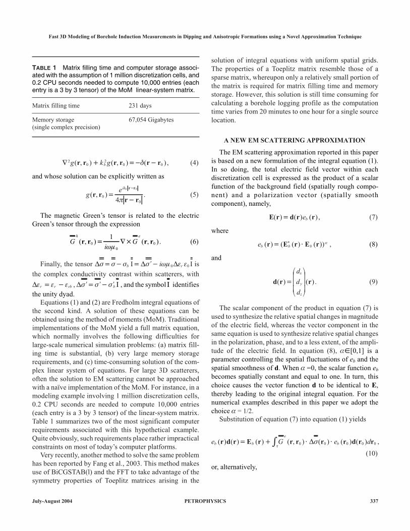
with a naïve implementation of the MoM. For instance, in a
modeling example involving 1 million discretization cells,
0.2 CPU seconds are needed to compute 10,000 entries
(each entry is a 3 by 3 tensor) of the linear-system matrix.
Table 1 summarizes two of the most significant computer
requirements associated with this hypothetical example.
Quite obviously, such requirements place rather impractical
constraints on most of today’s computer platforms.
Very recently, another method to solve the same problem
has been reported by Fang et al., 2003. This method makes
use of BiCGSTAB(l) and the FFT to take advantage of the
symmetry properties of Toeplitz matrices arising in the
solution of integral equations with uniform spatial grids.
The properties of a Toeplitz matrix resemble those of a
sparse matrix, whereupon only a relatively small portion of
the matrix is required for matrix filling time and memory
storage. However, this solution is still time consuming for
calculating a borehole logging profile as the computation
time varies from 20 minutes to one hour for a single source
location.
A NEW EM SCATTERING APPROXIMATION
The EM scattering approximation reported in this paper
is based on a new formulation of the integral equation (1).
In so doing, the total electric field vector within each
discretization cell is expressed as the product of a scalar
function of the background field (spatially rough compo-
nent) and a polarization vector (spatially smooth
component), namely,
E r d r r( ) ( ) ( ) ,� eb (7)
where
eb b b( ) ( ( ) ( )) ,*r E r E r� � � (8)
and
d r r( ) ( ) .�
�
�
���
�
�
���
d
d
d
x
y
z
(9)
The scalar component of the product in equation (7) is
used to synthesize the relative spatial changes in magnitude
of the electric field, whereas the vector component in the
same equation is used to synthesize relative spatial changes
in the polarization, phase, and to a less extent, of the ampli-
tude of the electric field. In equation (8), ��[0,1] is a
parameter controlling the spatial fluctuations of eb and the
spatial smoothness of d. When � =0, the scalar function eb
becomes spatially constant and equal to one. In turn, this
choice causes the vector function d to be identical to E,
thereby leading to the original integral equation. For the
numerical examples described in this paper we adopt the
choice � = 1/2.
Substitution of equation (7) into equation (1) yields
e G e db b
e
b( ) ( ) ( ) ( , ) ( ) ( ) ( ) ,r d r E r r r r r d r r� � � �� 0 0 0 0 0��
(10)
or, alternatively,
July-August 2004 PETROPHYSICS 337
Fast 3D Modeling of Borehole Induction Measurements in Dipping and Anisotropic Formations using a Novel Approximation Technique
TABLE 1 Matrix filling time and computer storage associ-ated with the assumption of 1 million discretization cells, and0.2 CPU seconds needed to compute 10,000 entries (eachentry is a 3 by 3 tensor) of the MoM linear-system matrix.
Matrix filling time 231 days
Memory storage 67,054 Gigabytes
(single complex precision)
d r d r r r rr
rd r( ) ( ) ( , ) ( )
( )
( )(� � � �
�
���
�
���b
eb
b
Ge
e0 0
0
0�� ) ,dr0�
(11)
where
d r E r e rb b b( ) ( ) / ( ) .� (12)
The new approximation stems directly from this last
integral equation. In the above expressions, eb embodies
relative changes in the magnitude of the internal electric
field due to the proximity of the EM source. The larger the
distance from the EM source to the scatterer, the less signif-
icant the spatial changes of eb within the scatterer. In the far
field, one would expect eb to be spatially constant within the
scatterer.
The spatial smoothness criterion necessary to accurately
describe vector d depends, to some extent, on the proximity
of the EM receiver to the scatterer. Equation (1) shows that
the simulation of EM scattering at the receiver location is
performed by propagating the internal scattering electrical
currents to the EM receiver location. In this case, the
propagator is given by the electric Green’s tensor,
Ge
R( , ) ,r r0
where rR is the EM receiver location and r0 is a point within
the scatterer. The effect of the propagator can also be
thought of as an operation wherein the scattering current,
��( ) ( )r E r0 0�
is spatially low-pass filtered (i.e. it is smoothed in space) to
provide the value of the electric field at the EM receiver
location. For a constant frequency, such a smoothing opera-
tion becomes more pronounced as the receiver recedes away
from the scatterer. In the case of a fixed transmitter-receiver
configuration, such as in borehole induction logging, the
propagator itself provides a precise measure of the degree of
smoothness necessary to compute accurate solutions of the
scattered EM field at the receiver location. In other words,
even though scattering currents may exhibit large spatial
variations within the scatterer, these spatial variations are
effectively smoothed when propagated to the receiver loca-
tion. Because of this important remark, it is only necessary
to calculate scattering currents with accuracies consistent
with those of the spatial smoothing properties of the propa-
gator.
The criterion adopted in this paper to control the degree
of spatial smoothness of the internal electric field consists
of discretizing the scatterer into a collection of blocks, each
block consisting of several cells. This procedure assumes
that within each block the d vector is constant, whereas the
scalar function is assumed variable within a block but con-
stant within a cell. Because of the choice of a uniform spa-
tial discretization grid, all cells exhibit the same shape and
size. The spatial distribution and size of blocks, however,
can be chosen in a more flexible manner. It is only required
that blocks be built to conform to cell boundaries. Finally,
the d vector associated with a given block is solved via
equation (11). Such a procedure gives rise to an over-deter-
mined (rectangular) complex linear system of equations for
the unknown vector d within all of the discretization
blocks. The rectangular, over-determined nature of the lin-
ear system of equations is due to the fact that the number of
blocks is, by construction, smaller than the number of cells.
Following a procedure described in the Appendix, the rect-
angular linear system is reduced to a 3Nx3N linear system
of equations where N is the number of blocks. This reduc-
tion of the size of the linear system substantially decreases
memory storage and CPU time requirements.
Additional savings in computer storage and CPU execu-
tion time are obtained with the use of a uniform spatial
discretization scheme and a Toeplitz matrix formulation.
When using uniform discretization grids, a Toeplitz matrix
is constructed for each discretization block. Matrix vector
multiplications are further accelerated using the FFT. Inter-
ested readers are referred to Fang et al., (2003) for technical
details on the implementation of the FFT to solve block
Toeplitz linear systems.
We remark that the spatial discretization of blocks and
cells adopted in this paper is of a Cartesian type. Moreover,
in an effort to properly model the borehole, the Cartesian
block discretization is chosen with orthogonal axes
conformal to the axis of the borehole (and hence conformal
to the axis of the logging instrument). Cell locations and
distances between a given cell and the axis of the borehole
are measured perpendicular to the borehole axis. For the
case of a non-conformal distribution of conductivity such
as, for instance, dipping anisotropic beds, a conductivity
averaging technique is used to assign a tensorial electrical
conductivity to a specific cell. In this paper, we adopt the
material averaging technique described by Wang and Fang
(2001) to assign an electrical conductivity tensor to a
particular cell.
ON THE CHOICE OF A VALUE OF BACKGROUND
ELECTRICAL CONDUCTIVITY
As emphasized above, the integral equation approxima-
tion introduced in this paper makes use of a Green’s tensor
defined over a homogeneous and isotropic unbounded
medium. The choice of the simplest possible Green’s tensor
is made to limit the complexity of the numerical computa-
tions associated with the integral equation solution.
338 PETROPHYSICS July-August 2004
Gao et al.
Another important reason for this choice is that the Green’s
tensor associated with a homogeneous and isotropic
unbounded medium remains space shift-invariant in all
three Cartesian coordinates. It is also emphasized that the
new approximation involves two conformal spatial
discretization volumes. The first one is constructed using
fine cells to describe the spatial variability of the scalar term
eb. In turn, the specific value of eb assigned to a given cell
depends on the assumed background model. The value of
background conductivity should be selected to provide the
largest possible accuracy within the practical limits of the
approximation.
The background conductivity should be some compro-
mise between the contribution of small and large conductiv-
ity values in the rock formation model, for example by min-
imizing the difference between the minimum and maximum
formation conductivity values using some weighted metric.
Extensive numerical experiments suggested that the geo-
metrical average of the minimum and maximum formation
conductivity values provided optimal results for the exam-
ples considered in this paper. This geometrical average is
given by
� � �b � �min max . (13)
The variables �min and �max in equation (13) are the mini-
mum and maximum, respectively, of all the conductivity
values considered in the numerical simulation.
Equation (13) is also suggested by studies in the theory
of effective media involving the electrical conductivity of
two-dimensional composites. It can be shown that a sym-
metric mixture of two components exhibits an effective
conductivity given by the geometric average of the conduc-
tivities of the constituent materials. Alternative procedures
could exist to choose an optimal background conductivity.
These could include weighted averages of the conductivity
distribution, where the weights would be determined by (a)
proximity to the source(s), (b) proximity to the receiver(s),
and (c) block volume. Yet another variation of equation (13)
could be constructed with averages of electrical conductiv-
ity or resistivity taken along orthogonal or arbitrary direc-
tions. The latter possibility is enticing but we choose not to
explore it in the present publication.
Quite obviously, the choice of background conductivity
other than that of the borehole conductivity causes the bore-
hole itself to become part of the anomalous conductivity
region. Because of this, memory and CPU requirements
increase when computing the internal electric field. Despite
such difficulties, numerical experiments show that the
choice of background conductivity different from that of
the borehole does not substantially compromise the effi-
ciency of the simulation algorithm. The small sacrifice in
computer efficiency is drastically outweighed by the gain in
numerical accuracy. Moreover, the implementation of the
integral equation algorithm described in this paper makes
use of 3D FFTs that can only be implemented on a uniform
and spatially continuous discretization grid. The
discretization does include the borehole region, and there-
fore the algorithm does not explicitly enforce a choice of
background conductivity equal to the borehole conductiv-
ity.
SENSITIVITY TO THE CHOICE OF SPATIAL
DISCRETIZATION
As emphasized above, there are two levels of spatial
discretization involved in the computation of the integral
equation approximation described in this paper. A fine cell
structure is first constructed to describe the spatial varia-
tions within the scatterer of the scalar factor eb contained in
equations (10) or (11). The relative spatial variations of this
factor are primarily controlled by the proximity of the EM
source to the scatterers. On the other hand, a relatively
larger conformal block structure is constructed to describe
the spatial variations of vector d. A given block in the
discretization scheme of vector d is composed of several
cells used to spatially discretize the scalar factor eb. The
specific choice of block and cell structure can have a signif-
icant influence on the performance of the approximation.
The strategy chosen in this paper to construct block
structures is one in which small blocks are placed in close
proximity to the borehole, the transmitter(s), and/or the
receiver(s). Small discretization blocks are required near
receivers because an accurate representation of the polar-
ization vector is needed in those blocks to properly account
for the relative large influence of the dyadic Green’s tensor
when propagating the internal electric field to receiver loca-
tions. Larger blocks are used to discretize the remaining
spatial regions in the scattering rock formations.
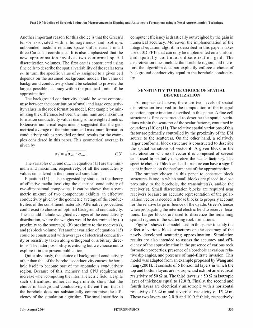
Figure 1 shows the model used in this paper to study the
effect of various block structures on the accuracy of the
newly developed scattering approximation. Simulation
results are also intended to assess the accuracy and effi-
ciency of the approximation in the presence of various rock
formation properties, presence of a borehole at various rela-
tive dip angles, and presence of mud-filtrate invasion. This
model was adapted from an example proposed by Wang and
Fang (2001). It consists of 5 horizontal layers in which the
top and bottom layers are isotropic and exhibit an electrical
resistivity of 50 ��m. The third layer is a 50 ��m isotropic
layer of thickness equal to 12.0 ft. Finally, the second and
fourth layers are electrically anisotropic with a horizontal
resistivity of 3 ��m and a vertical resistivity of 15 ��m.
These two layers are 2.0 ft and 10.0 ft thick, respectively.
July-August 2004 PETROPHYSICS 339
Fast 3D Modeling of Borehole Induction Measurements in Dipping and Anisotropic Formations using a Novel Approximation Technique
Mud-filtrate invasion may also be present within these last
two layers, with an invasion length equal to 36 in, and with
the resistivity in the invaded zone equal to 3 ��m. The
diameter of the borehole is equal to 8.0 in. and its resistivity
is equal to 1 ��m.
Simulation results are computed for borehole deviations
of 0° and 60° for two cases of rock formation model: First,
the formation is assumed to have no invasion and no bore-
hole, i.e. to consist of a 1D stack of layers. The second
model does assume a borehole and invasion, with the
parameters described in the preceding paragraph. We com-
pare simulation results with those obtained using a 1D code
(identified as “1D” in the corresponding figures) and the 3D
finite difference simulation algorithm (identified as “3D
FDM” in the figures) developed by Wang and Fang (2001).
The 3D FDM simulation results reported in this paper have
been validated and benchmarked for accuracy by Wang and
Fang (2001). In the descriptions and figures below, the
identifier “3DIE Appr.” is used to designate simulation
results obtained with the new approximation developed in
this paper.
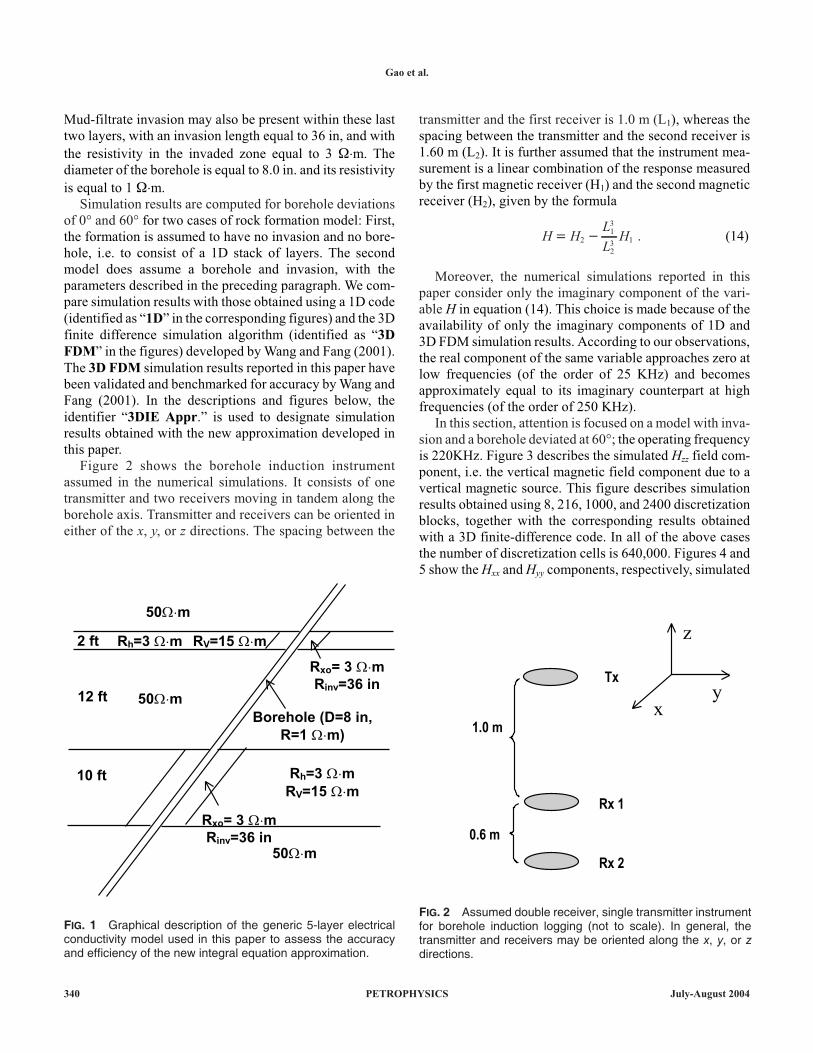
Figure 2 shows the borehole induction instrument
assumed in the numerical simulations. It consists of one
transmitter and two receivers moving in tandem along the
borehole axis. Transmitter and receivers can be oriented in
either of the x, y, or z directions. The spacing between the
transmitter and the first receiver is 1.0 m (L1), whereas the
spacing between the transmitter and the second receiver is
1.60 m (L2). It is further assumed that the instrument mea-
surement is a linear combination of the response measured
by the first magnetic receiver (H1) and the second magnetic
receiver (H2), given by the formula
H HL
LH� �2
13
23 1 . (14)
Moreover, the numerical simulations reported in this
paper consider only the imaginary component of the vari-
able H in equation (14). This choice is made because of the
availability of only the imaginary components of 1D and
3D FDM simulation results. According to our observations,
the real component of the same variable approaches zero at
low frequencies (of the order of 25 KHz) and becomes
approximately equal to its imaginary counterpart at high
frequencies (of the order of 250 KHz).
In this section, attention is focused on a model with inva-
sion and a borehole deviated at 60°; the operating frequency
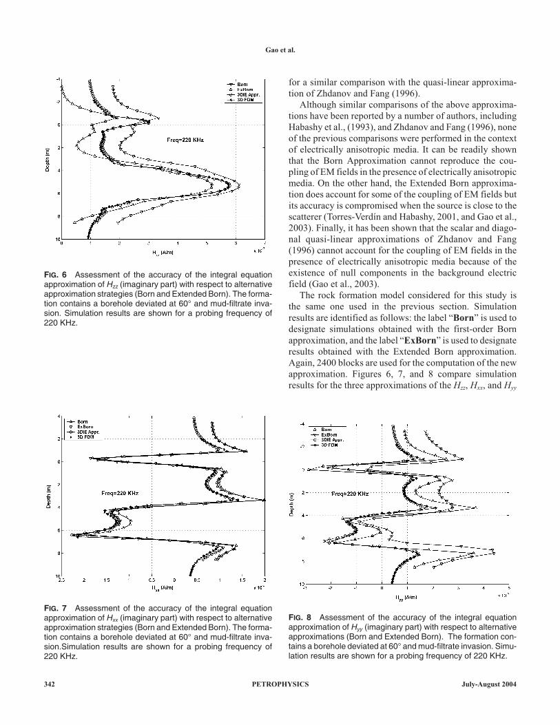
is 220KHz. Figure 3 describes the simulated Hzz field com-
ponent, i.e. the vertical magnetic field component due to a
vertical magnetic source. This figure describes simulation
results obtained using 8, 216, 1000, and 2400 discretization
blocks, together with the corresponding results obtained
with a 3D finite-difference code. In all of the above cases
the number of discretization cells is 640,000. Figures 4 and
5 show the Hxx and Hyy components, respectively, simulated
340 PETROPHYSICS July-August 2004
Gao et al.
10 ft
50��m
Rh=3 ��m RV=15 ��m
Rxo= 3 ��m
Rinv=36 in50��m
Rh=3 ��m
RV=15 ��m
Rxo= 3 ��m
Rinv=36 in50��m
Borehole (D=8 in,
R=1 ��m)
2 ft
12 ft
FIG. 1 Graphical description of the generic 5-layer electricalconductivity model used in this paper to assess the accuracyand efficiency of the new integral equation approximation.
Tx
Rx 1
Rx 2
1.0 m
0.6 m
xy
z
FIG. 2 Assumed double receiver, single transmitter instrumentfor borehole induction logging (not to scale). In general, thetransmitter and receivers may be oriented along the x, y, or z
directions.
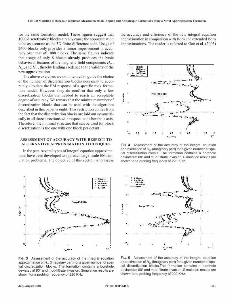
for the same formation model. These figures suggest that
1000 discretization blocks already cause the approximation
to be as accurate as the 3D finite-difference code. Usage of
2400 blocks only provides a minor improvement in accu-
racy over that of 1000 blocks. The same figures indicate
that usage of only 8 blocks already produces the basic
behavioral features of the magnetic field components Hxx ,
Hyy, and Hzz , thereby lending credence to the validity of the
new approximation.
The above exercises are not intended to guide the choice
of the number of discretization blocks necessary to accu-
rately simulate the EM response of a specific rock forma-
tion model. However, they do confirm that only a few
discretization blocks are needed to reach an acceptable
degree of accuracy. We remark that the minimum number of
discretization blocks that can be used with the algorithm
described in this paper is eight. This restriction comes from
the fact that the discretization blocks are laid out symmetri-
cally in all three directions with respect to the borehole axis.
Therefore, the minimal structure that can be used for block
discretization is the one with one block per octant.
ASSESSMENT OF ACCURACY WITH RESPECT TO
ALTERNATIVE APPROXIMATION TECHNIQUES
In the past, several types of integral equation approxima-
tions have been developed to approach large-scale EM sim-
ulation problems. The objective of this section is to assess
the accuracy and efficiency of the new integral equation
approximation in comparison with Born and extended Born
approximations. The reader is referred to Gao et al. (2003)
July-August 2004 PETROPHYSICS 341
Fast 3D Modeling of Borehole Induction Measurements in Dipping and Anisotropic Formations using a Novel Approximation Technique
FIG. 3 Assessment of the accuracy of the integral equationapproximation of Hzz (imaginary part) for a given number of spa-tial discretization blocks. The formation contains a boreholedeviated at 60° and mud-filtrate invasion. Simulation results areshown for a probing frequency of 220 KHz
FIG. 4 Assessment of the accuracy of the integral equationapproximation of Hxx (imaginary part) for a given number of spa-tial discretization blocks. The formation contains a boreholedeviated at 60° and mud-filtrate invasion. Simulation results areshown for a probing frequency of 220 KHz.
FIG. 5 Assessment of the accuracy of the integral equationapproximation of Hyy (imaginary part) for a given number of spa-tial discretization blocks.The formation contains a boreholedeviated at 60° and mud-filtrate invasion. Simulation results areshown for a probing frequency of 220 KHz.
for a similar comparison with the quasi-linear approxima-
tion of Zhdanov and Fang (1996).
Although similar comparisons of the above approxima-
tions have been reported by a number of authors, including
Habashy et al., (1993), and Zhdanov and Fang (1996), none
of the previous comparisons were performed in the context
of electrically anisotropic media. It can be readily shown
that the Born Approximation cannot reproduce the cou-
pling of EM fields in the presence of electrically anisotropic
media. On the other hand, the Extended Born approxima-
tion does account for some of the coupling of EM fields but
its accuracy is compromised when the source is close to the
scatterer (Torres-Verdín and Habashy, 2001, and Gao et al.,
2003). Finally, it has been shown that the scalar and diago-
nal quasi-linear approximations of Zhdanov and Fang
(1996) cannot account for the coupling of EM fields in the
presence of electrically anisotropic media because of the
existence of null components in the background electric
field (Gao et al., 2003).
The rock formation model considered for this study is
the same one used in the previous section. Simulation
results are identified as follows: the label “Born” is used to
designate simulations obtained with the first-order Born
approximation, and the label “ExBorn” is used to designate
results obtained with the Extended Born approximation.
Again, 2400 blocks are used for the computation of the new
approximation. Figures 6, 7, and 8 compare simulation
results for the three approximations of the Hzz, Hxx, and Hyy
342 PETROPHYSICS July-August 2004
Gao et al.
FIG. 6 Assessment of the accuracy of the integral equationapproximation of Hzz (imaginary part) with respect to alternativeapproximation strategies (Born and Extended Born). The forma-tion contains a borehole deviated at 60° and mud-filtrate inva-sion. Simulation results are shown for a probing frequency of220 KHz.
FIG. 7 Assessment of the accuracy of the integral equationapproximation of Hxx (imaginary part) with respect to alternativeapproximation strategies (Born and Extended Born). The forma-tion contains a borehole deviated at 60° and mud-filtrate inva-sion.Simulation results are shown for a probing frequency of220 KHz.
FIG. 8 Assessment of the accuracy of the integral equationapproximation of Hyy (imaginary part) with respect to alternativeapproximations (Born and Extended Born). The formation con-tains a borehole deviated at 60° and mud-filtrate invasion. Simu-lation results are shown for a probing frequency of 220 KHz.
field components, respectively. Simulation results summa-
rized in these figures indicate a superior performance of the
new approximation with respect to the Born and extended
Born approximations.
NUMERICAL EXAMPLES
Additional rock formation models and probing frequen-
cies have been considered to further assess the accuracy and
efficiency of the new approximation. These include: (a) a
1D formation that has no borehole and no invasion, with the
source direction deviated at an angle of 0° and 60°, (b) a 3D
formation with invasion and a borehole deviated at an angle
of 0° and 60°. The probing frequencies considered in the
simulations are 20 KHz and 220 KHz. Although the main
purpose of this paper is to assess the accuracy and effi-
ciency of the new approximation in the simulation of bore-
hole EM logging measurements, some petrophysical com-
ments are provided when interpreting the simulation exam-
ples. The intent of such comments is to assess the physical
consistency of the approximation.
The spatial discretization grid constructed for the simu-
lations reported in this paper consists of 80 cells in the x
-direction, 80 cells in the y-direction, and 100 cells in the z-
direction. Cell sizes are kept uniform and equal to 0.1 m. In
total, 2400 blocks are used for the discretization of the mod-
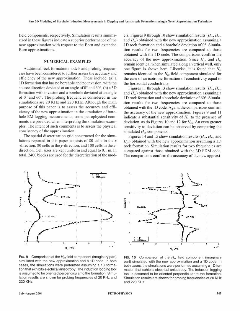
els. Figures 9 through 10 show simulation results (Hzz, Hxx,
and Hyy) obtained with the new approximation assuming a
1D rock formation and a borehole deviation of 0°. Simula-
tion results for two frequencies are compared to those
obtained with the 1D code. The comparisons confirm the
accuracy of the new approximation. Since Hxx and Hyy
remain identical when simulated along a vertical well, only
one figure is shown here. Likewise, it is found that Hzz
remains identical to the Hzz field component simulated for
the case of an isotropic formation of conductivity equal to
the horizontal conductivity.
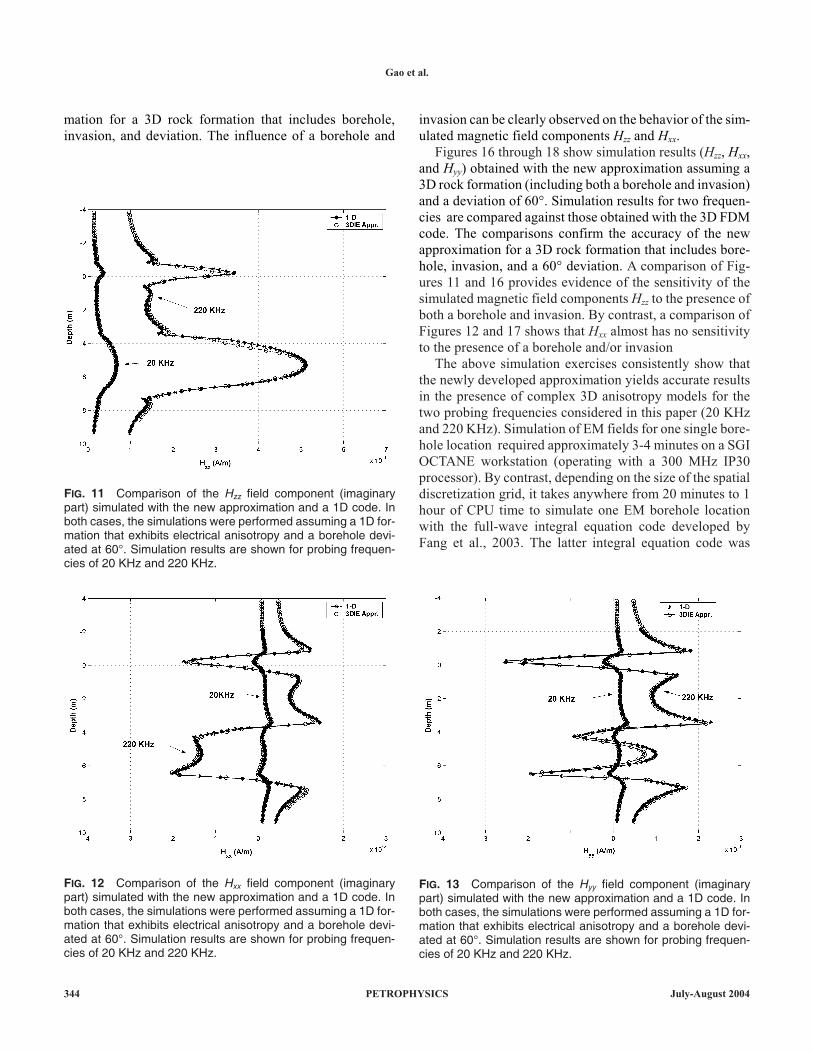
Figures 11 through 13 show simulation results (Hzz, Hxx,
and Hyy) obtained with the new approximation assuming a
1D rock formation and a borehole deviation of 60°. Simula-
tion results for two frequencies are compared to those
obtained with the 1D code. Again, the comparisons confirm
the accuracy of the new approximation. Figures 9 and 11
indicate a substantial sensitivity of Hzz to the presence of
deviation, as do Figures 10 and 12 for Hxx. An even greater
sensitivity to deviation can be observed by comparing the
simulated Hyy components.
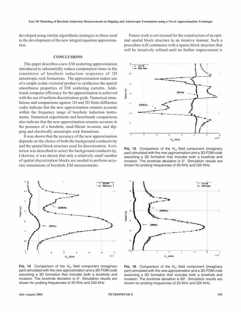
Figures 14 and 15 show simulation results (Hzz, Hxx, and
Hyy) obtained with the new approximation assuming a 3D
rock formation. Simulation results for two frequencies are
compared against those obtained with the 3D FDM code.
The comparisons confirm the accuracy of the new approxi-
July-August 2004 PETROPHYSICS 343
Fast 3D Modeling of Borehole Induction Measurements in Dipping and Anisotropic Formations using a Novel Approximation Technique
FIG. 9 Comparison of the Hzz field component (imaginary part)simulated with the new approximation and a 1D code. In bothcases, the simulations were performed assuming a 1D forma-tion that exhibits electrical anisotropy. The induction logging toolis assumed to be oriented perpendicular to the formation. Simu-lation results are shown for probing frequencies of 20 KHz and220 KHz.
FIG. 10 Comparison of the Hxx field component (imaginarypart) simulated with the new approximation and a 1D code. Inboth cases, the simulations were performed assuming a 1D for-mation that exhibits electrical anisotropy. The induction loggingtool is assumed to be oriented perpendicular to the formation.Simulation results are shown for probing frequencies of 20 KHzand 220 KHz
mation for a 3D rock formation that includes borehole,
invasion, and deviation. The influence of a borehole and
invasion can be clearly observed on the behavior of the sim-
ulated magnetic field components Hzz and Hxx.
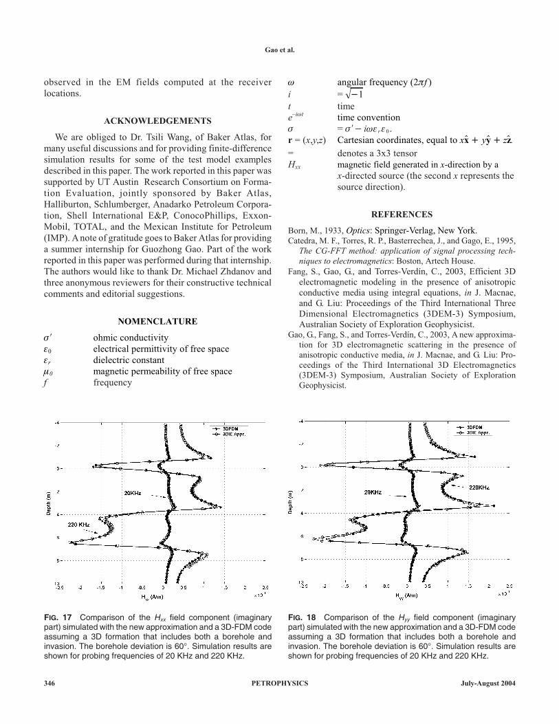
Figures 16 through 18 show simulation results (Hzz, Hxx,
and Hyy) obtained with the new approximation assuming a
3D rock formation (including both a borehole and invasion)
and a deviation of 60°. Simulation results for two frequen-
cies are compared against those obtained with the 3D FDM
code. The comparisons confirm the accuracy of the new
approximation for a 3D rock formation that includes bore-
hole, invasion, and a 60° deviation. A comparison of Fig-
ures 11 and 16 provides evidence of the sensitivity of the
simulated magnetic field components Hzz to the presence of
both a borehole and invasion. By contrast, a comparison of
Figures 12 and 17 shows that Hxx almost has no sensitivity
to the presence of a borehole and/or invasion
The above simulation exercises consistently show that
the newly developed approximation yields accurate results
in the presence of complex 3D anisotropy models for the
two probing frequencies considered in this paper (20 KHz
and 220 KHz). Simulation of EM fields for one single bore-
hole location required approximately 3-4 minutes on a SGI
OCTANE workstation (operating with a 300 MHz IP30
processor). By contrast, depending on the size of the spatial
discretization grid, it takes anywhere from 20 minutes to 1
hour of CPU time to simulate one EM borehole location
with the full-wave integral equation code developed by
Fang et al., 2003. The latter integral equation code was
344 PETROPHYSICS July-August 2004
Gao et al.
FIG. 11 Comparison of the Hzz field component (imaginarypart) simulated with the new approximation and a 1D code. Inboth cases, the simulations were performed assuming a 1D for-mation that exhibits electrical anisotropy and a borehole devi-ated at 60°. Simulation results are shown for probing frequen-cies of 20 KHz and 220 KHz.
FIG. 12 Comparison of the Hxx field component (imaginarypart) simulated with the new approximation and a 1D code. Inboth cases, the simulations were performed assuming a 1D for-mation that exhibits electrical anisotropy and a borehole devi-ated at 60°. Simulation results are shown for probing frequen-cies of 20 KHz and 220 KHz.
FIG. 13 Comparison of the Hyy field component (imaginarypart) simulated with the new approximation and a 1D code. Inboth cases, the simulations were performed assuming a 1D for-mation that exhibits electrical anisotropy and a borehole devi-ated at 60°. Simulation results are shown for probing frequen-cies of 20 KHz and 220 KHz.
developed using similar algorithmic strategies to those used
in the development of the new integral equation approxima-
tion.
CONCLUSIONS
This paper describes a new EM scattering approximation
introduced to substantially reduce computation times in the
simulation of borehole induction responses of 3D
anisotropic rock formations. The approximation makes use
of a simple scalar-vectorial product to synthesize the spatial
smoothness properties of EM scattering currents. Addi-
tional computer efficiency for the approximation is achieved
with the use of uniform discretization grids. Numerical simu-
lations and comparisons against 1D and 3D finite-difference
codes indicate that the new approximation remains accurate
within the frequency range of borehole induction instru-
ments. Numerical experiments and benchmark comparisons
also indicate that the new approximation remains accurate in
the presence of a borehole, mud-filtrate invasion, and dip-
ping and electrically anisotropic rock formations.
It was shown that the accuracy of the new approximation
depends on the choice of both the background conductivity
and the spatial block structure used for discretization. A cri-
terion was described to select the background conductivity.
Likewise, it was shown that only a relatively small number
of spatial discretization blocks are needed to perform accu-
rate simulations of borehole EM measurements.
Future work is envisioned for the construction of an opti-
mal spatial block structure in an iterative manner. Such a
procedure will commence with a sparse block structure that
will be iteratively refined until no further improvement is
July-August 2004 PETROPHYSICS 345
Fast 3D Modeling of Borehole Induction Measurements in Dipping and Anisotropic Formations using a Novel Approximation Technique
FIG. 14 Comparison of the Hzz field component (imaginarypart) simulated with the new approximation and a 3D-FDM codeassuming a 3D formation that includes both a borehole andinvasion. The borehole deviation is 0°. Simulation results areshown for probing frequencies of 20 KHz and 220 KHz
FIG. 16 Comparison of the Hzz field component (imaginarypart) simulated with the new approximation and a 3D-FDM codeassuming a 3D formation that includes both a borehole andinvasion. The borehole deviation is 60°. Simulation results areshown for probing frequencies of 20 KHz and 220 KHz.
FIG. 15 Comparison of the Hxx field component (imaginarypart) simulated with the new approximation and a 3D-FDM codeassuming a 3D formation that includes both a borehole andinvasion. The borehole deviation is 0°. Simulation results areshown for probing frequencies of 20 KHz and 220 KHz.
observed in the EM fields computed at the receiver
locations.
ACKNOWLEDGEMENTS
We are obliged to Dr. Tsili Wang, of Baker Atlas, for
many useful discussions and for providing finite-difference
simulation results for some of the test model examples
described in this paper. The work reported in this paper was
supported by UT Austin Research Consortium on Forma-
tion Evaluation, jointly sponsored by Baker Atlas,
Halliburton, Schlumberger, Anadarko Petroleum Corpora-
tion, Shell International E&P, ConocoPhillips, Exxon-
Mobil, TOTAL, and the Mexican Institute for Petroleum
(IMP). A note of gratitude goes to Baker Atlas for providing
a summer internship for Guozhong Gao. Part of the work
reported in this paper was performed during that internship.
The authors would like to thank Dr. Michael Zhdanov and
three anonymous reviewers for their constructive technical
comments and editorial suggestions.
NOMENCLATURE
�� ohmic conductivity
0 electrical permittivity of free space
r dielectric constant
�0 magnetic permeability of free space
f frequency
� angular frequency (2�f )
i = �1
t time
e–i�t time convention
� = ��� � i r 0.
r = (x,y,z) Cartesian coordinates, equal to x y z� � �x y z� � .
= denotes a 3x3 tensor
Hxx magnetic field generated in x-direction by a
x-directed source (the second x represents the
source direction).
REFERENCES
Born, M., 1933, Optics: Springer-Verlag, New York.Catedra, M. F., Torres, R. P., Basterrechea, J., and Gago, E., 1995,
The CG-FFT method: application of signal processing tech-
niques to electromagnetics: Boston, Artech House.
Fang, S., Gao, G., and Torres-Verdín, C., 2003, Efficient 3D
electromagnetic modeling in the presence of anisotropic
conductive media using integral equations, in J. Macnae,
and G. Liu: Proceedings of the Third International Three
Dimensional Electromagnetics (3DEM-3) Symposium,
Australian Society of Exploration Geophysicist.Gao, G., Fang, S., and Torres-Verdín, C., 2003, A new approxima-
tion for 3D electromagnetic scattering in the presence of
anisotropic conductive media, in J. Macnae, and G. Liu: Pro-
ceedings of the Third International 3D Electromagnetics
(3DEM-3) Symposium, Australian Society of Exploration
Geophysicist.
346 PETROPHYSICS July-August 2004
Gao et al.
FIG. 17 Comparison of the Hxx field component (imaginarypart) simulated with the new approximation and a 3D-FDM codeassuming a 3D formation that includes both a borehole andinvasion. The borehole deviation is 60°. Simulation results areshown for probing frequencies of 20 KHz and 220 KHz.
FIG. 18 Comparison of the Hyy field component (imaginarypart) simulated with the new approximation and a 3D-FDM codeassuming a 3D formation that includes both a borehole andinvasion. The borehole deviation is 60°. Simulation results areshown for probing frequencies of 20 KHz and 220 KHz.
Gao. G., Torres-Verdín C., and Fang S., 2003, Fast 3D modeling of
borehole induction data in dipping and anisotropic formations
using a novel approximation technique, paper VV in 44th
Annual Logging Symposium Transactions: Society of
Professional Well Log Analysts.
Gao, G., Torres-Verdín, C., Habashy, T. M., and Fang, S., 2002,
Approximations to electromagnetic scattering based on natural
preconditioners of the method-of-moments’ stiffness matrix:
applications to the probing of subsurface rock formations, pre-
sented at 2002 IEEE AP-S International Symposium: URSI
Radio Science Meeting.
Sleijpen, G. L. G. and Fokkema, D. R., 1993, BiCGSTAB(l) for lin-
ear equations involving unsymmetric matrices with complex
spectrum: Electronic Transactions on Numerical Analysis, vol.
1, p. 11–32.
Habashy, T. M., Groom, R. W., and Spies, B., 1993, Beyond the
Born and Rytov approximations: a nonlinear approach to elec-
tromagnetic scattering: J. Geophys. Res., vol. 98, no. B2, p.
1759–1775.
Hohmann, G. W, 1975, Three-dimensional induced polarization
and electromagnetic modeling: Geophysics, vol. 40, no. 2, p.
309–324.
Hursan, G. and Zhdanov, M. S., 2002, Contraction integral equa-
tion method in 3-D em scattering modeling: Radio Science, vol.
37, no. 6, p. 1089.
Torres-Verdín, C. and Habashy, T. M., 1994, Rapid 2.5-dimen-
sional forward modeling and inversion via a new nonlinear
scattering approximation: Radio Science, vol. 29, no. 4, p.
1051–1079.
Wang, T. and Fang, S., 2001, 3-D electromagnetic anisotropy
modeling using finite differences: Geophysics, vol. 66, no. 5, p.
1386–1398.
Wannamaker, P. E., Hohmann, G. W., SanFilipo, W.A., 1983, Elec-
tromagnetic modeling of three-dimensional bodies in layered
earth using integral equations: Geophysics, vol. 49, no. 1, p.
60–74.
Xiong, Z., 1992, Electromagnetic modeling of 3-D structures by
the method of system iteration using integral equations: Geo-
physics, vol. 57, no. 12, p. 1556–1561.
Zhdanov, M. S. and Fang, S., 1996, Quasi-linear approximation in
3-D electromagnetic modeling: Geophysics, vol. 61, no. 3, p.
646–665.
Zhdanov, M. S., 2002, Geophysical inverse theory and regulariza-
tion theory problems: Elsevier, Amsterdam, London, New
York, Tokyo, 628 p.
APPENDIX
ALGORITHMIC IMPLEMENTATION OF THE NEW
EM SCATTERING APPROXIMATION
We first divide the scattering domain into N blocks, with
Vn being the spatial region occupied by the n-th block, and
d r d r( ) ( ) ,��
� n n
n
N
P1
(A.1)
where
PV
elsewheren
n( ) .r
r�
����
1
0(A.2)
Substituting equation (A.1) into equation (10) yields
e G e db
e
b n bV
n
N
n
( ) ( ) ( , ) ( ) ( ) ( )r d r r r r r r d E r� � ����
0 0 0 0
1
�� .
(A.3)
Because the conductivity tensor is constant within a
given block one can rewrite equation (A.3) as
e G e db
e
b n n bV
n
N
n
( ) ( ) ( , ) ( ) ( ) .r d r r r r r d E r� � ����
0 0 0
1
��
(A.4)
We now divide block Vn into Pn cells and proceed to
match the incident fields at each cell location, rm. Equation
(A.4) becomes
e G d eb m m
e
m bp
Vp
P
n
N
nP
n
( ) ( ) ( , )r d r r r r��
!
"
#$���
��
0 0
11
��n n b md E r� ( ) .
(A.5)
For each cell, we define
G G d
G G G
G G G
G G G
e
mV
xx xy xz
yx yy yz
zx zy zz
nP
� �
�
!!� ( , )r r r0 0
!
"
#
$$$, (A.6)
and
B Gebp� . (A.7)
Equation (A.4) then becomes
e Bb m m np
p
P
n
N
n n b m
n
( ) ( ) ( ) .r d r d E r��
!
"
#$ �
��
��11
�� (A.8)
Using matrix notation, equation (A.7) can be written as
( ) ,A C S d RM N M N N N N M3 3 3 3 3 3 3 1 3 1� � � � �� � (A.9)
where M is the number of cells and
July-August 2004 PETROPHYSICS 347
Fast 3D Modeling of Borehole Induction Measurements in Dipping and Anisotropic Formations using a Novel Approximation Technique
A
A
A
A
A
N N
NN
�
�
!!!!!!
"
#
$$$$$$
� �
11
22
1 1
� . (A.10)
In (A.10), each submatrix Aii , i = 1%N is associated
with the background field within a given block, and it has
the dimensions 3P � 3. For example
A
e
e
e
e
e
e
b
p
b
p
b
p
b
p
b
p
b
p
p
p
11
11
11
11
11
11
1
0 0
0 0
0 0
0 0
0 0
0 0
� � � �
p1
�
�
���������
�
�
���������
, (A.11)
d d d d d d dx y z Nx Ny NzT� ( , , , , , , ) ,1 1 1 � (A.12)
and
C
C C C C
C C C C
C C C
N N
N N
N N N
�
�
�
� �
11 12 1 1 1
21 22 2 1 2
11 12
�
�
� � � � �
� � � �
�
�
!!!!!!
"
#
$$$$$$
1 1 1
1 2 1
N N N
N N NN NN
C
C C C C�
. (A.13)
Each submatrix
C C Bij ijP
p
Pj
� �� �[ ]3 3
represents the contribution from the j-th block on the i-th
cell.
Also,
S
S
S
S
S
N N
NN
�
�
!!!!!!
"
#
$$$$$$
� �
11
22
1 1
� , (A.14)
where each submatrix Sii (i = 1 � N) contains the average
conductivity tensor for each block. The size of this
submatrix is 3 � 3, namely, S ii i��� . The conductivity
averaging technique used to assemble the entries Sii of
matrix S is the one described by Wang and Fang (2001).
Finally,
R E E E E E Eb x b y b z bMx bMy bMzT� ( , , , , , , ) .1 1 1 � (A.15)
To solve the over-determined complex linear system of
equations represented by equation (A.9), we pre-multiply
both sides of equation (A.9) by matrix A* to obtain
( ) ,* * *A A A CS d A R� � (A.16)
where matrix A* is the transpose conjugate of matrix A.
Because the matrices A*A, A*C, and A*R are all independent
of conductivity, they can be stored in hard-disk memory
prior to performing the computations. Specifically, when
the conductivity distribution changes with a change of loca-
tion of the induction-logging instrument, it is only necessary
to construct a new conductivity matrix. The remaining
matrices included in equation (A.16) will not change with a
change in instrument location.
It is pointed out that equation (A.16) is different from the
least-squares solution of the over-determined complex lin-
ear system of equations described by equation (A.9). The
way to obtain a least-squares solution of the over-deter-
mined linear system (A.9) is to pre-multiply both sides of
the linear system by the matrix (A – CS)*. However, we
remark that such an operation may involve substantial com-
puter resources. The rationale for using equation (A.16)
instead of the standard least-squares solution is as follows.
From inspection of equations (A.6), (A.7) and (A.13) one
can conclude that, in general, the entries of matrix A are
much larger than those of matrix CS. One can easily show
that the entries of matrix C involve the entries of matrix A
multiplied by values derived from the Green’s tensor that,
in turn, are customarily much smaller than 1. In view of the
above, equation (A.16) remains an accurate and expedient
alternative to the least-squares solution of equation (A.9).
Extensive numerical experiments have confirmed the prac-
tical validity of equation (A.16).
348 PETROPHYSICS July-August 2004
Gao et al.
ABOUT THE AUTHORS
Guozhong Gao is currently a Graduate Research Assistant
and a PhD candidate in the Department of Petroleum and
Geosystems Engineering at the University of Texas at Austin.
He obtained his Bachelor degree and Master degree from
Southwest Petroleum Institute (China) and Beijing Petroleum
University in 1996 and 2000, respectively, all in Applied Geo-
physics. His current research interests include algorithm devel-
opment for electromagnetic scattering, especially for modeling
the inhomogeneous and anisotropic earth formations, inverse
scattering, and formation evaluation. Email: gaogz@hotmail.
com.
Carlos Torres-Verdín received a PhD in Engineering
Geoscience from the University of California, Berkeley, in
1991. During 1991–1997, he held the position of Research Sci-
entist with Schlumberger-Doll Research. From 1997–1999, he
was Reservoir Specialist and Technology Champion with YPF
(Buenos Aires, Argentina). Since 1999, he is an Assistant Pro-
fessor with the Department of Petroleum and Geosystems
Engineering of The University of Texas at Austin, where he
conducts research in formation evaluation and integrated reser-
voir characterization. He has served as Guest Editor for Radio
Science, and is currently a member of the Editorial Board of the
Journal of Electromagnetic Waves and Applications, and an
associate editor for Petrophysics (SPWLA) and the SPE Jour-
nal. Email: [email protected]
Sheng Fang is currently a senior scientist and has been
working on well logging applications with Baker Atlas since
1998. He received his BS (1984) and MS (1989) degrees in
applied geophysics from China University of Geosciences
(CUG) and his PhD (1998) degree in geophysics from the Uni-
versity of Utah (UU). His main research interests are in numeri-
cal simulation, practical inversion, and in developing data pro-
cessing and interpretation techniques for different logging
tools including resistivity, nuclear magnetic resonance (NMR),
and pulse neutron capture (PNC) measurements. Email:
July-August 2004 PETROPHYSICS 349
Fast 3D Modeling of Borehole Induction Measurements in Dipping and Anisotropic Formations using a Novel Approximation Technique