Family Law E¤ects on Divorce, Fertility and Child Investment1

Meta BrownResearch and Statistics Group

Federal Reserve Bank of New York33 Liberty Street

New York, NY 10045e-mail: Meta.Brown@ny.frb.org

Christopher J. FlinnDepartment of Economics,New York University269 Mercer StreetNew York, NY 10003

e-mail: christopher.�inn@nyu.edu

Collegio Carlo AlbertoMoncalieri, Italy

July 2011

1This research was supported in part by grants from the National Science Foundation, Collegio CarloAlberto and the C.V. Starr Center for Applied Economics at NYU. We are grateful to the CHRR for accessto NLSY 1979 cohort Geocode data, and to Hugette Sun for sharing her extensive child support guideline li-brary. Steven Laufer contributed indispensible components of the programming framework, and James Mabliprovided excellent research assistance. David Blau, Hanming Fang, Ariel Pakes, Ken Wolpin and seminarparticipants at the Institute for Research on Poverty, NYU, Virginia, UNC-Greensboro, Wisconsin, Torino,the Society for Economic Dynamics, ESPE, the American Economic Association Meetings, the UNC/DukeConference on Labor, Health and Aging, the Minnesota Applied Micro Workshop and the Stanford Institutefor Theoretical Economics provided valuable comments. The views and opinions o¤ered in this paper do notnecessarily re�ect the position of the Federal Reserve Bank of New York or the Federal Reserve System.

Abstract

In order to assess the child welfare impact of policies governing divorced parenting, such as child

support orders, child custody and placement regulations, and marital dissolution standards, one

must consider their in�uence not only on the divorce rate but also on spouses�fertility choices and

child investments. We develop a continuous time model of marriage, fertility and parenting, with the

main goal being the determination of how policies toward divorce in�uence outcomes for husbands,

wives and children. Estimates are derived for model parameters of interest using the method of

simulated moments, and simulations based on the model explore the e¤ects of changes in custody

allocations and child support standards on outcomes for intact and divided families. Simulations

indicate that, while a small decrease in the divorce rate may be induced by a signi�cant child

support hike, the major e¤ect of child support levels for both intact and divided households is on

the distribution of welfare between parents. Simulated divorce, fertility, test scores and parental

welfare all increase with a move toward shared physical placement. Finally, the simulations indicate

that children�s interests are not necessarily best served by minimizing divorced parenting.

JEL codes: J12, J13, J18

1 Introduction

Divorced parenting in the U.S. is regulated through a combination of laws controlling marital

dissolution, child custody and placement, and the assignment and enforcement of child support

obligations. The primary objective of these activities is to increase the well-being of children

and parents, and the divorce rate is often regarded as a �rst order measure of the success of

family law. The rationale for this focus is the preponderance of empirical evidence that suggests

that children living in households without both biological parents are more likely to su¤er from

behavioral problems and have lower levels of a broad range of achievement indicators measured at

various points over the life cycle (see, e.g., Haveman and Wolfe 1995). Recent empirical studies of

unilateral divorce laws and child support enforcement have isolated the e¤ects of changes in such

legal structures on divorce rates (e.g., Friedberg 1998 and Gruber 2004, Wolfers 2006 and Nixon

1997). A complete picture of the in�uence of family law on family members�welfare would include

an understanding of the mechanisms by which family law changes in�uence fertility, child outcomes,

and the distribution of resources within the family, in addition to divorce rates. Toward that end,

this paper models the interaction of married couples in the shadow of existing divorce regulations

in terms of decisions regarding fertility, child investment and divorce.

A standing problem for research on parents�dynamic child investment activities is the frequent

absence of data on fathers. Much of what we have learned about parents� dynamic decision-

making, therefore, has been in the context of a mother�s (or mother and father�s, assuming a unitary

objective) individual dynamic optimization problem, as in Bernal (2008), Bernal and Keane (2011),

Blau and van der Klaauw (2008) and Liu, Mroz and van der Klaauw (2010).

Where the subject is the in�uence of divorce regulations on the family, however, the distinct

choices of mothers and fathers are paramount. It is virtually impossible to understand the in�uence

of potential child support, for example, on fertility, investment and divorce decisions by studying

the mother�s perspective in isolation. Hence we model the choices of mothers and fathers as an

ongoing, simultaneous-move game. Our model and data begin from the date of marriage, which,

while excluding a substantial and non-random segment of parents, has the bene�t of granting access

to similar information on the mother and father when early fertility, investment and divorce choices

are being made.

In taking this approach, we draw on an extensive empirical literature on marriage dynamics,

including Aiyagari, Greenwood and Guner (2000), Brien, Lillard and Stern (2006), Chiappori,

Fortin and Lacroix (2002), and others. This literature emphasizes the repeated interaction of a

husband and wife in deciding whether to continue a marriage and the allocation of household

resources.1 What we seek to add to existing analyses is the impact of the (endogenous) arrival and

development of a shared child and its role, as well as the role of exposure to divorced parenting

1Caucutt, Guner and Knowles (2002) is a rare example of an existing study of marriage dynamics (including amarriage market), fertility and child expenditures. However, their framework is a three period overlapping generationsmodel, and their object of interest is the life-cycle timing of fertility, where we model spouses�decisions in continuoustime throughout the fertility and childrearing process, and our ultimate interest is in child outcomes.

1

regulation, in marital status dynamics.

A closely related paper is Tartari (2007). It includes a substantially enriched child quality

production technology relative to the one that we estimate, and it focuses less on capturing the

institutional structure and e¤ects of family law.

The model allows spouses to make (simultaneous) choices regarding marriage continuation,

fertility, and, where relevant, individual investments in children, in a continuous time framework.

A match value of marriage is drawn from a population distribution and evolves stochastically

over time. Fertility choices are in�uenced by both the expected bene�t from the presence of the

child and expectations regarding the duration of the marriage, given the state of the marriage

quality process. Child quality, re�ected by cognitive ability in the empirical implementation of the

model, progresses as a result of both endogenous parental investment and marital status choices

and exogenous productivity factors. Marital dissolution may result from changes in marriage match

quality, child presence and quality, and when the child reaches �independence�(in the sense of the

model, which is explained below). Thus the full history of marriage values and child investments

determines current marital status and child investment levels. If the history of child investments

and marriage values is poorer for the marginal marriage than it is for the representative marriage,

then, all else equal, the child welfare gain associated with the continuation of the marginal marriage

is smaller than that associated with the continuation of the representative marriage. An important

objective of our analysis is to study the welfare impacts of variations in family law, which are possible

to assess under our assumptions regarding the determination of the utility levels of husbands, wives,

and (potential) children.

The model is estimated utilizing data from the National Longitudinal Study of Youth�s 1979

cohort (NLSY-79) using the method of simulated moments (MSM). Computational issues arise, and

we employ a technique similar to the one independently developed by Imai, Jain and Ching (2009)

to permit simultaneous solution and estimation of this complex dynamic game. Variation across

state and intertemporal variation in marital dissolution standards and child support guidelines aids

the identi�cation of model parameters, and allows us to rely on more than model structure when

estimating parameters used in our comparative statics exercises and policy analysis. While prior

research has made extensive use of variation in laws regulating the granting of divorce across states,

the use of states�widely varying child support guidelines to generate informative variation in child

support orders is a relatively new practice.2

The model we estimate is extremely parsimonious (which is a positive way to say �stylized�).

Nevertheless, we �nd that the model is able to �t most of the many features of the data used in esti-

mation to a very satisfactory degree, with a few notable exceptions. That gives us some con�dence

in using the estimated model to perform comparative statics exercises and welfare analysis.

An important feature of our model is the incorporation of a fertility decision. In the compar-

ative statics exercises we �nd that family law potentially has an important impact not only the

2Existing analysis of individual exposure to child support liability using the guidelines is, to our knowledge, limitedto Sun (2005). We are very grateful to Hugette Sun for sharing her child support guideline library and for her adviceon working with the guideline data.

2

achievement levels of children from intact and nonintact households, but even more fundamentally

on the number of children born and the characteristics of the households having them. The e¤ects

of variations in child contact time allocations in the divorce state have a particularly strong impact

on fertility, with 20 percent fewer households having children within 10 years from the date of the

marriage when the father is given no time as opposed to when he is allocated 50 percent of the

time. These variations also impact the (�nal) distribution of child quality not only through their

impact on the incentive to invest in children but also due to the fact that only parents expecting

high quality children and a stable marriage will have children in such an �extreme�family law envi-

ronment. Conversely, we �nd that the e¤ect of wide variation in child support orders has a modest

impact on fertility decisions and child quality. This seems largely due to the diminishing marginal

utility of consumption and the perfect substitutability of parental investments in the stochastic

child quality production function.

Our analysis concludes with an attempt to determine optimal family law parameters using a

Benthamite social welfare function. The main problem with employing such an approach in our

modeling framework is that the set of agents is endogenous due to the presence of the fertility

decision. We are able to make some progress by merging the seminal approaches to this question

found in Blackorby et al. (1995) and Golosov et al. (2007). Our simulation exercise adopts an ex

ante welfare criterion (evaluated at the time of marriage) which only involves the agents always

present, the husband and wife. We �nd that the welfare objective is optimized under 50/50 physical

placement, a 20 percent child support rate and a bilateral divorce standard. Custody arrangements

generally dominate the welfare ordering, with the divorce standard being of minimal net welfare

consequence.

The plan of the paper is as follows. In Section 2 we describe some of the �marriage life-cycle�

patterns in the data with which we hope our model is consistent. In Section 3 we develop the

details of the model. Section 4 describes our rather complex estimation method and presents a

fairly rigorous discussion of the manner in which primitive parameters are identi�ed. In Section

5 we describe the data in detail and present descriptive statistics for our sample. The estimates

of the primitive parameters and assessment of model �t are found in Section 6. In Section 7 we

describe comparative statics results and our attempt to determine optimal family law. Section 8

concludes.

2 Divorce and Fertility Dynamics in the NLSY-79

The di¢ culty of isolating policy e¤ects on marriage, fertility and child investment is perhaps best

illustrated in data on families� dynamic choices. We turn to our estimation sample of families,

described in more detail in Section 5. In broad terms, the sample includes all of the women of the

NLSY-79 cohort who ever marry and who have no children at the date of �rst marriage. To this we

add the requirement that we observe complete marriage and fertility histories for the women, some

income data, and a few other variables required to carry out the estimation of the model. Figure

3

1 describes the rate at which �rst children arrive to the NLSY-79 women in this sample. On the

horizontal axis is the number of years since the date of marriage; on the vertical is the proportion

of women who experience a birth at the given number of years since the marriage date. We look at

fertility trajectories from the marriage date separately by the number of years left in the marriage.

The darkest, dashed line represents fertility rates among couples who will remain married 10 years

from the date in question. With the exception of the �rst year of marriage, their fertility rate

lies everywhere above the fertility rates of couples who are approaching divorce.3 The irregularly

dashed line represents couples who will be divorced by the next year. Their fertility rate is the

lowest of all of the groups in most years. The solid and dotted lines represent couples who will

divorce in two and three years, respectively. Their fertility rates lie below the married-in-10-years

rates, and, for the most part, above the fertility rates of those who will divorce in one year. Overall

we see a strong negative association between remaining time in the marriage and the fertility rate.

If these briefer marriages are fundamentally of lower quality, or marginal, marriages, then it would

appear that marginal marriages produce fewer children.

The children of stable marriages in the sample demonstrate substantially higher cognitive ability

than the children of marriages headed for divorce. Figure 2 depicts children�s average age-normed

math score on the Peabody Individual Achievement Test (PIAT) as a function of years since their

parents were married. Test score averages for children whose parents will still be married in three

years lie above those for children of divorce and those for children whose parents will be divorced

in three years (with the single exception of the sixth year of marriage), and the rate of increase

in their average test scores outpaces those of the other groups. One interesting fact that emerges

from this exercise is that the average test scores for children of marriages approaching divorce are

everywhere the same as or worse than the scores for children of divorce. It appears that, in this

NLSY-79 sample, weak marriages are associated not just with child attainments that resemble

those in divorce more than they resemble child attainment in stable marriages, but instead with

child attainments that are frequently worse than those associated with divorce.

Of course, this in no way implies that low marriage quality causes either low fertility or low

child attainment. Low fertility, for example, could cause an otherwise stable marriage to end.

Figure 3 depicts divorce rates beginning from the date of marriage for those with and without

children. For the �rst seven years of marriage, the divorce rate for couples without children lies

far above the divorce rate for couples with children. At around 8 years, the divorce rates for

both groups stabilize at roughly 2 percent per year, and the two groups� divorce rates remain

comparable thereafter.4 Hence we see a strong negative association between fertility and divorce,

and the direction of causation is far from clear. One hypothesis is that some type of fundamental

heterogeneity in marriage quality in�uences both marital status and fertility decisions, leading to

3Note that these are rolling categorizations, so that the group of couples who will divorce in two years as of thesecond year of marriage is the same group as those who will divorce in one year as of the third year of marriage, andso on.

4The positive association between the presence of children and marital stability at the early stages of marriageand the eventual diminution of the relationship is consistent with the �ndings of Waite and Lillard (1991).

4

this strong negative association between fertility and divorce. Another is that marital status and

fertility are simultaneously determined, in that the return to producing and investing in children as

marriage-speci�c capital increases with the duration of marriage, and at the same time the presence

of a child increases the return to marriage, contributing to its stability.5

In such an environment, the in�uence of policies that alter the costs and bene�ts of divorce

for the two spouses depends heavily on the relative importance of basic heterogeneity in marriage

quality and the interdependence of fertility and marital stability in families�decisions. For example,

a marriage that is marginal in some fundamental sense may be held together by a policy adjustment,

and still this marginal marriage may produce less in the way of children or child investment than

the average marriage might. Conversely, if the heterogeneity in underlying marriage quality is not

large and if fertility and divorce decisions are responsive to economic and policy incentives, then

policy changes may have extensive welfare-improving e¤ects on fertility and divorce rates. A model

that permits both fundamental heterogeneity in marriage quality and feedback among marriage

stability, fertility and child investment is therefore required in order to understand the in�uence of

divorce policy on the well-being of wives, husbands and children.

3 A Model of Child Investment and Divorce Decisions

There exist two decision-making agents in our model, spouses s = 1; 2. The model is set in

continuous time, and the instantaneous utility function of spouse s is given by

us(cs; k; �; d) = �s ln(cs) + (1� �s)� s(d)p(ln(k) + �) + (1� d)�; s = 1; 2; (1)

where cs is the consumption of a private good by spouse s, d is an indicator variable that takes

the value 1 if the spouses are divorced, � is a marriage-speci�c match value, the value of which can

change over time, p is an indicator taking the value 1 if a child is present, k is the value of child

quality, which is weakly greater than 1 when the spouses have had a child, � s(d) is the amount of

contact that the parent has with the child given the divorce status of the parents; �s 2 (0; 1) isthe preference weight on private consumption and � is a constant welfare cost or bene�t of child

presence.6 We assume throughout that the price of private consumption is �xed at 1 for both

parents.

In the absence of a child, if the spouses are married their instantaneous utilities are given by

us(cs; 1; �; 0) = �s ln(cs) + �; s = 1; s;

5See Lillard and Waite (1993) for a statistical model of the simultaneity of divorce and fertility choices.6The parameter � will be free to take positive or negative values. It may be interpreted as a welfare cost or bene�t

of child presence or, equivalently in this speci�cation, as a scaling factor relating the value of child quality to thevalue of consumption.

5

and if divorced their utilities are given by

us(cs; 1; �; d) = �s ln(cs); s = 1; 2:

In the presence of a child, the utility derived from current child quality by each parent is

modi�ed according to the amount of contact the parent has with the child in each marriage state.

We assume that when married the parents enjoy complete and concurrent access to the child�s time;

without loss of generality, �1(0) = �2(0) = 1: Though their intrinsic valuation of the child remains

the same in the divorce state, the fact that the child becomes an �excludable�good after divorce

reduces the utility �ows that parents receive from any given level of child quality.7 We assume that

parents share time with the child in divorce, implying �1(1) + �2(1) = 1 and � s(1) � 0; s = 1; 2;and that physical custody and visitation allocations are fully anticipated and set exogenously with

respect to parental behaviors.8

Each spouse has a baseline income �ow at any moment in time, which is denoted by ys: The

actual income under the control of individual s is state-dependent in the following sense. Spouses

receive incomes of Ys(y1; y2; a); s = 1; 2 and where a = d � p. When a = 0; each spouse has

his or her own income, so that Ys(y1; y2; 0) = ys; while when a = 1 the income of ex-spouse 1 is

Y1(y1; y2; 1) = (1� �)y1 and the income of ex-spouse 2 is Y2(y1; y2; 1) = y2 + �y1: We assume that

spouse 1 bears the child support obligation.9 ;10

The dynamics of the model are as follows.

1. The model begins at the time of marriage. Spouses are initially childless. If both spouses

agree to attempt to have a child, then a child arrives at rate > 0: We de�ne the state

variable f 2 f0; 1g to indicate whether this fertility process is active, with f = 1 representingan active fertility process. The fertility process may only be active in the married state.

2. There are M possible values of marriage quality, with � 2 �� = f�1; :::; �Mg; where �1 <�2 < : : : < �M : At the onset of marriage, there is an initial marriage quality draw: During

the marriage, there may occur changes to the marriage quality value, which we model as a

(continuous time) random walk. Match quality increases arrive at rate e +; as long as currentmatch quality �m is less than �M : The arrival of a match quality increase leads with certainty

to a new match quality of �m+1. Symmetrically, match quality decreases arrive at rate e �;as long as �m > �1; and the arrival of a decrease in match quality leads to a drop from �m to

7This, in fact, is the only way in which our model re�ects losses of economies of scale after divorce. Other quasi-�xed costs, such as housing, utilities, etc., which are signi�cant sources of scale economies when three individuals liveunder one roof, are not included in the this modeling set up.

8See, for example, Fox and Kelly (1995) for details on custody determination.9The empirical analysis assigns spouse 1 as the male and spouse 2 as the female in the observed marriage. We

�nd that a small minority of child support payments �ow from mothers to fathers in the NLSY-79.10By assuming that there is no transfer ordered after a divorce if the couple is childless, we are essentially assuming

away alimony. Alimony is increasingly uncommon in U.S. divorce cases. According to Case et al. (2003), for example,5 (4.2) percent of 1977 PSID (in 1997) mothers received alimony.

6

�m�1. For convenience of notation we de�ne

+(�m) =

( e + where 1 � m < M

0 otherwiseand �(�m) =

( e � where 1 < m �M

0 otherwise.

The values of +(�m) and �(�m) determine the degree of persistence in marriage quality

over any given time interval:

3. There are B possible baseline income �ow levels for each spouse, with ys 2 �ys = fy1s ; :::; yBs g;where 0 < y1s < ::: < yBs : Each spouse begins marriage with an own-income �ow of ys: Over

time, there may occur shocks to each spouse�s income state. Spouse s receives positive income

shocks at rate ~�+s as long as current income y

bs is less than y

Bs ; and receives negative shocks

at rate ~��s as long as y

bs > y1s : Analogously to the case of marriage quality, a negative income

shock leads to a decrease from ybs to yb�1s and a positive income shock leads to an increase

from ybs to yb+1s : We de�ne

�+s (ybs) =

(~�+s where 1 � b < B

0 otherwiseand ��s (y

bs) =

(~��s where 1 < b � B

0 otherwise.:

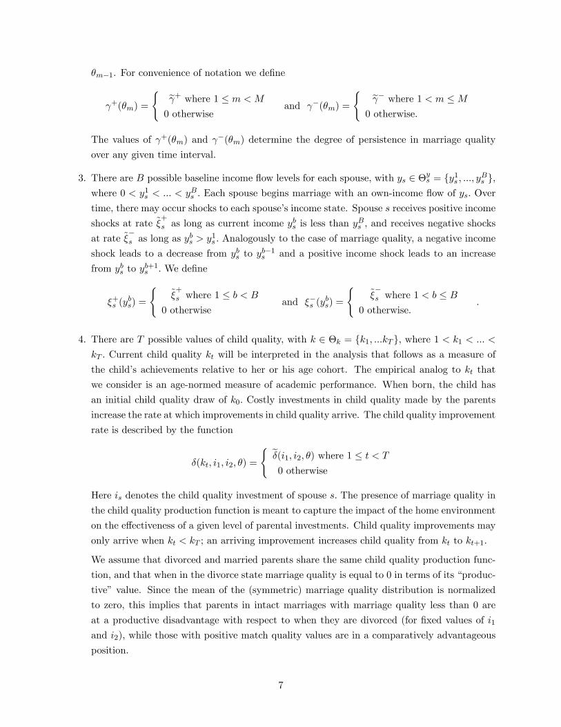
4. There are T possible values of child quality, with k 2 �k = fk1; :::kT g; where 1 < k1 < ::: <

kT : Current child quality kt will be interpreted in the analysis that follows as a measure of

the child�s achievements relative to her or his age cohort. The empirical analog to kt that

we consider is an age-normed measure of academic performance. When born, the child has

an initial child quality draw of k0: Costly investments in child quality made by the parents

increase the rate at which improvements in child quality arrive. The child quality improvement

rate is described by the function

�(kt; i1; i2; �) =

( e�(i1; i2; �) where 1 � t < T

0 otherwise

Here is denotes the child quality investment of spouse s: The presence of marriage quality in

the child quality production function is meant to capture the impact of the home environment

on the e¤ectiveness of a given level of parental investments. Child quality improvements may

only arrive when kt < kT ; an arriving improvement increases child quality from kt to kt+1:

We assume that divorced and married parents share the same child quality production func-

tion, and that when in the divorce state marriage quality is equal to 0 in terms of its �produc-

tive�value. Since the mean of the (symmetric) marriage quality distribution is normalized

to zero, this implies that parents in intact marriages with marriage quality less than 0 are

at a productive disadvantage with respect to when they are divorced (for �xed values of i1and i2), while those with positive match quality values are in a comparatively advantageous

position.

7

5. Child quality setbacks occur at exogenous rate e�; and lead to a decline in child quality fromkt to kt�1 whenever 1 < t � T . We de�ne

�(kt) =

( e� where 1 < t � T

0 where t = 1:

6. Finally, the child may attain functional independence at the current age-normed child quality,

in which case the child quality improvement process ends. The parents enjoy a terminal

value that increases with the current child quality level and continues to depend on the

parents�marital status.11 Termination of the investment process occurs at exogenous rate �;

state variable e 2 f0; 1g indicates the current investment condition, and equals 1 when theinvestment process has been terminated.

The child quality production function described by dynamic elements 4-6 is of necessity peculiar

to our continuous-time, simultaneous investment modelling approach. However, it can be related

to leading models of child investment. Cunha and Heckman (2007) and Cunha, Heckman, Lochner,

and Masterov (2006) argue that a variety of skills that children must develop are subject to "critical

periods" early in life, and hence much of intellectual development is accomplished by the time the

child reaches school age. Hopkins and Bracht (1975), for example, demonstrate that IQ is stable by

the age of 10 or so, suggesting that the critical period for intellectual development occurs by this

time. Further, Cunha and Heckman, Cunha et al., and Cunha, Heckman and Schennach (2010)

emphasize the importance of both cognitive and non-cognitive skill acquisition to child outcomes,

along with the importance of "dynamic complementarity" and "self-productivity" of skill levels

in ongoing skill production. Todd and Wolpin (2003, 2007) consider cognitive skill formation,

and argue from a di¤erent perspective for the importance of both current and lagged inputs to

the ongoing production process. They demonstrate the importance of allowing for unobserved

endowment e¤ects and the endogeneity of inputs to child skill production.

Like Todd and Wolpin, we restrict attention to cognitive skill.12 Our empirical work de�nes ktbased on an age-normed measure of child attainment. Hence, the manner in which we allow for

self-productivity and the role of lagged investments is very particular, in that prior investments and

attainment determine the child�s current place among a population of children, each of whom has

a history of investments and attainment that may contribute to his subsequent progress. Growth

in the child�s outcome measure in this instance will depend on the relative productivity of own

and peers�current and lagged investments, and past attainments, allowing for the possibility, in

a somewhat circumscribed sense, of nonlinearities in the dynamic production of absolute skill

levels. The initial conditions that we specify when estimating the model directly address the need

11An alternative approach to �nalizing the child investment process would be to impose a �xed time horizon of 18or 21 years, after which children achieve independence. The drawback to this approach is that it generates strategicmanipulations by parents approaching the date of independence that we �nd unrealistic.12Our empirical meausure, discussed below in Section 5, is in fact more narrow than theirs in the space of cognitive

skills.

8

to account for unobserved endowment heterogeneity, and the model accounts for endogeneity of

investments in determining absolute skill level in a speci�c manner. Finally, the investment period

that we model begins at birth. Our empirical implementation focuses on progress from birth

through a set of tests that are completed for most sample children before the age of ten, be�tting

an analysis of cognitive skill production under the prescriptions of the literature.

In modeling the behavior of married and divorced parents an important speci�cation choice

is the manner in which spouses interact. One may assume that spouses interact cooperatively or

noncooperatively.13 It is unclear that ex-spouses are able to interact in a manner that achieves

the Pareto frontier. In a model that moves though married and divorced states, if cooperation

is ever attained in marriage it is unclear how spouses�mode of interaction might transition from

such cooperation in marriage to the potential cooperation failures of divorce, or how the presence

of children might in�uence interactions in divorce. One might assume cooperation throughout,

though this is certainly unsatisfying for childless divorced spouses and, moreover, rules out any

e¤ect of marital dissolution standards on divorce rates under conventional speci�cations. One

might assume noncooperative interaction throughout, though this may be unsatisfying for the

case of young spouses starting a family. More complex approaches include allowing spouses to

choose the current mode of interaction as events progress, following Flinn (2000), or specifying

population heterogeneity in spouses�mode of interaction, following Eckstein and Lifshitz (2009).

Though the latter approaches are appealing, they would add a great deal of complexity to an already

complex model. For the above reasons, and given standing evidence of marriage dissolution standard

e¤ects on divorce rates in Friedberg, Gruber and elsewhere, we choose to assume noncooperative

interaction throughout. In our discussion of the theoretical results we dedicate some attention to

the e¤ects of this modeling choice. Finally, we assume that spouses�investment strategies constitute

a Markov Perfect Equilibrium.14

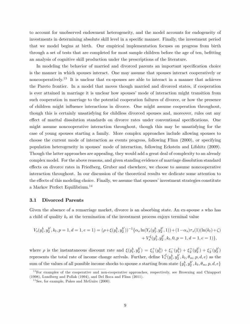
3.1 Divorced Parents

Given the absence of a remarriage market, divorce is an absorbing state. An ex-spouse s who has

a child of quality kt at the termination of the investment process enjoys terminal value

Vs(yb1; y

b02 ; kt; p = 1; d = 1; e = 1) = (�+�(y

b1; y

b02 ))

�1f�s ln(Ys(yb1; yb02 ; 1))+(1��s)� s(1)(ln(kt)+�)

+ V �s (yb1; y

b02 ; kt; 0; p = 1; d = 1; e = 1)g;

where � is the instantaneous discount rate and �(yb1; yb02 ) = �+1 (y

b1) + ��1 (y

b1) + �+2 (y

b02 ) + ��2 (y

b02 )

represents the total rate of income change arrivals. Further, de�ne V �s (yb1; yb02 ; kt; �m; p; d; e) as the

sum of the values of all possible income shocks to spouse s starting from state fyb1; yb02 ; kt; �m; p; d; eg

13For examples of the cooperative and non-cooperative approaches, respectively, see Browning and Chiappori(1998), Lundberg and Pollak (1994), and Del Boca and Flinn (2011).14See, for example, Pakes and McGuire (2000).

9

multiplied by the shocks�instantaneous probabilities, so that

V �s (yb1; y

b02 ; kt; 0; p = 1; d = 1; e = 1) = �+1 (y

b1)V1(y

b+11 ; yb

02 ; kt; p = 1; d = 1; e = 1)

+ ��1 (yb1)V1(y

b�11 ; yb

02 ; kt; p = 1; d = 1; e = 1) + �

+2 (y

b02 )V2(y

b1; y

b0+12 ; kt; p = 1; d = 1; e = 1)

+ ��2 (yb02 )V2(y

b1; y

b0�12 ; kt; p = 1; d = 1; e = 1):

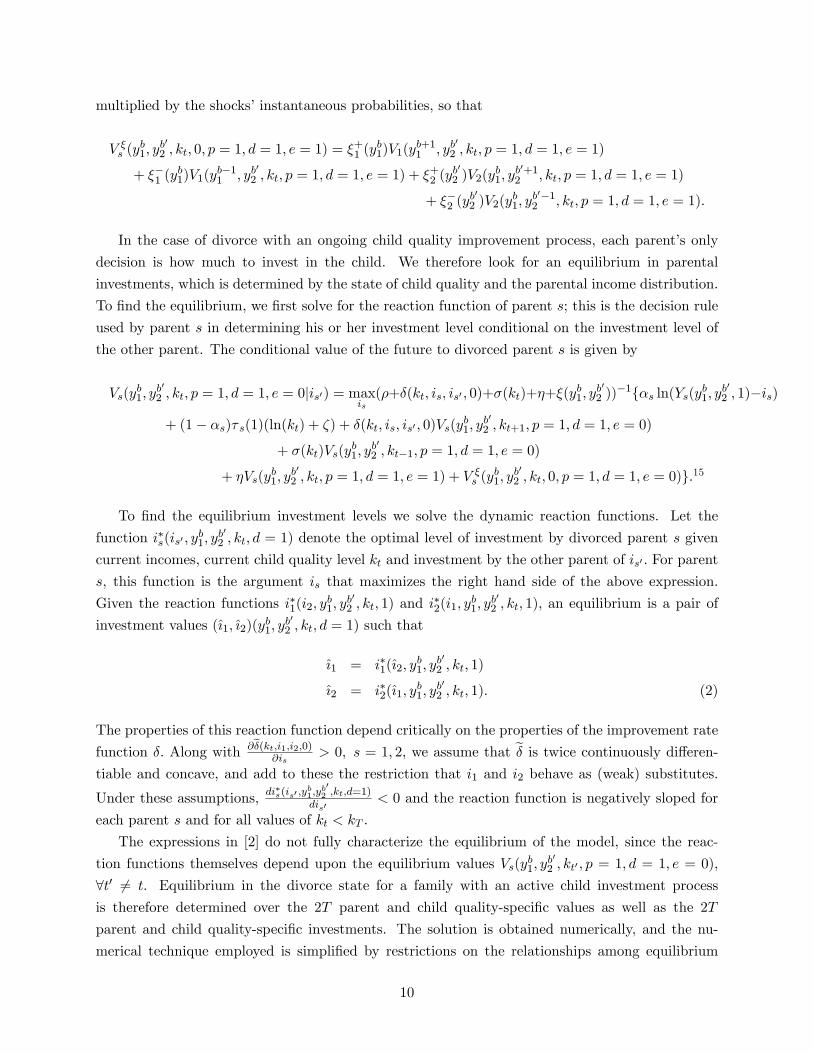
In the case of divorce with an ongoing child quality improvement process, each parent�s only

decision is how much to invest in the child. We therefore look for an equilibrium in parental

investments, which is determined by the state of child quality and the parental income distribution.

To �nd the equilibrium, we �rst solve for the reaction function of parent s; this is the decision rule

used by parent s in determining his or her investment level conditional on the investment level of

the other parent. The conditional value of the future to divorced parent s is given by

Vs(yb1; y

b02 ; kt; p = 1; d = 1; e = 0jis0) = max

is(�+�(kt; is; is0 ; 0)+�(kt)+�+�(y

b1; y

b02 ))

�1f�s ln(Ys(yb1; yb02 ; 1)�is)

+ (1� �s)� s(1)(ln(kt) + �) + �(kt; is; is0 ; 0)Vs(yb1; yb02 ; kt+1; p = 1; d = 1; e = 0)

+ �(kt)Vs(yb1; y

b02 ; kt�1; p = 1; d = 1; e = 0)

+ �Vs(yb1; y

b02 ; kt; p = 1; d = 1; e = 1) + V

�s (y

b1; y

b02 ; kt; 0; p = 1; d = 1; e = 0)g:15

To �nd the equilibrium investment levels we solve the dynamic reaction functions. Let the

function i�s(is0 ; yb1; y

b02 ; kt; d = 1) denote the optimal level of investment by divorced parent s given

current incomes, current child quality level kt and investment by the other parent of is0 : For parent

s, this function is the argument is that maximizes the right hand side of the above expression.

Given the reaction functions i�1(i2; yb1; y

b02 ; kt; 1) and i

�2(i1; y

b1; y

b02 ; kt; 1); an equilibrium is a pair of

investment values ({1; {2)(yb1; yb02 ; kt; d = 1) such that

{1 = i�1({2; yb1; y

b02 ; kt; 1)

{2 = i�2({1; yb1; y

b02 ; kt; 1): (2)

The properties of this reaction function depend critically on the properties of the improvement rate

function �: Along with @e�(kt;i1;i2;0)@is

> 0; s = 1; 2; we assume that e� is twice continuously di¤eren-tiable and concave, and add to these the restriction that i1 and i2 behave as (weak) substitutes.

Under these assumptions; di�s(is0 ;y

b1;y

b02 ;kt;d=1)

dis0< 0 and the reaction function is negatively sloped for

each parent s and for all values of kt < kT :

The expressions in [2] do not fully characterize the equilibrium of the model, since the reac-

tion functions themselves depend upon the equilibrium values Vs(yb1; yb02 ; kt0 ; p = 1; d = 1; e = 0);

8t0 6= t. Equilibrium in the divorce state for a family with an active child investment process

is therefore determined over the 2T parent and child quality-speci�c values as well as the 2T

parent and child quality-speci�c investments. The solution is obtained numerically, and the nu-

merical technique employed is simpli�ed by restrictions on the relationships among equilibrium

10

values arising from the theory and the use of the 2T values of terminal child qualities. Given the

ordering of child qualities and the possibility of setbacks when the investment process is active,

we know that Vs(yb1; yb02 ; kT ; p = 1; d = 1; e = 1) dominates the divorce-state values of (a) all ter-

minal child qualities kt such that t < T and (b) all non-terminal child qualities. Additionally,

Vs(yb1; y

b02 ; kt; p = 1; d = 1; e) increases monotonically with kt for both e = 0 and 1. The numerical

solution produces equilibrium investment levels f{1(yb1; yb02 ; kt; d = 1); {2(y

b1; y

b02 ; kt; d = 1)ggTt=1 and

value functions fV1(yb1; yb02 ; kt; p = 1; d = 1; e = 0); V2(y

b1; y

b02 ; kt; p = 1; d = 1; e = 0)gTt=1:

3.2 Married Parents

The experiences they will have if they enter the divorce state can meaningfully a¤ect the investment

decisions of forward-looking married parents. In particular, currently married parents who believe

that divorce is likely in the near future will make investment decisions that look more like those

made by divorced parents than will couples who believe that divorce is a remote possibility.

We must specify the manner in which divorce decisions are made. Under our assumption of

noncooperative behavior, these decisions are not, in general, e¢ cient. The nature of the decisions

depends critically on legal statutes. We consider two di¤erent cases: one in which it is enough for

one of the parents to ask for a divorce for the couple to enter the divorce state and the second in

which both parents must agree to the divorce for it to occur. These cases are commonly termed

unilateral and bilateral divorce regimes. In the empirical component, we link this solution standard

to prevailing state-year divorce laws.16 Given a divorce standard, we de�ne Qs(yb1; yb02 ; kt; �m; p; e)

as the value to spouse s of the marital status chosen in equilibrium by both spouses in state

(yb1; yb02 ; kt; �m; p; e): For ease of exposition we suppress any indication of the state of divorce law in

the remainder of this section, but note that the full equilibrium computation includes solution for

both divorce law states.

The derivation of the married parents�equilibrium is similar to that of the divorced parents�

equilibrium, with one major di¤erence being the search for an equilibrium in divorce decisions as

well as investments and values. As before, we begin with the value of a terminated child investment

16We �nd that solutions of the model assuming either bilateral or unilateral divorce laws, with or without allowingside payments, generate only small di¤erences in predicted behavior. This appears to be in large part the result of thenarrow range of child and marriage quality levels at which parents disagree over the divorce decision for reasonablevalues of the primitive parameters. Since previous research documents non-negligible e¤ects on divorce rates ofstates�adoption of unilateral divorce laws, we estimate under the assumptions of noncooperative behavior and noside payments in order to let the model accomodate any important behavior di¤erences by divorce law existing inthe data to the extent possible.

11

process at kt for spouse s:

Vs(yb1; y

b02 ; kt; �m; p = 1; d = 0; e = 1) = (�+

+(�m) + �(�m) + �(y

b1; y

b02 ))

�1n�s ln(y

bs)

+ (1� �s)(ln(kt) + �) + �m + +(�m)Qs(yb1; yb02 ; kt; �m+1; p = 1; e = 1)

+ �(�m)Qs(yb1; y

b02 ; kt; �m�1; p = 1; e = 1)

+V �s (yb1; y

b02 ; kt; �m; p = 1; d = 0; e = 1)

o:

(3)

In this case, the only possible arriving updates are to the marriage match value, �, and

the spouses� income levels: Since both spouses� welfare levels are increasing in child and mar-

riage quality, an increase in marriage quality (at rate +(�m)) cannot lead to a divorce, so that

Qs(yb1; y

b02 ; kt; �m+1; p = 1; e = 1) corresponds to the value of marriage at those state variables.

However, a decrease in marriage quality (at rate �(�m)) may lead to a divorce or to marriage

continuation.

Next, given the current child quality level and match value, we solve for the equilibrium invest-

ment levels and associated values for each parent conditional on the continuation of the marriage.

As in the divorce case, using the reaction functions we can de�ne a pair of equilibrium investment

levels and parent-speci�c state values associated with marriage that are given by

({1; {2)(yb1; y

b02 ; kt; �m; d = 0); (V1; V2)(y

b1; y

b02 ; kt; �m; p = 1; d = 0; e = 0): (4)

The investment equilibrium depends on the current marriage quality both through its direct in�u-

ence on the productivity of child investment and through its e¤ect on the anticipated duration of

the parents�marriage, which partially determines the expected gain associated with an increase in

child quality.

With the spouses�equilibrium investments in the child found as in [4], the value to spouse s of

marriage, a child with an ongoing child improvement process, and child quality kt is

Vs(yb1; y

b02 ; kt; �m; p = 1; d = 0; e = 0) = (�+

+(�m) + �(�m) + �(kt; {s; {s0 ; �m) + �(kt) + �

+ �(yb1; yb02 ))

�1f�s ln(ybs � {s) + (1� �s)(ln(kt) + �) + �m+ +(�m)Qs(y

b1; y

b02 ; kt; �m+1; p = 1; e = 0) +

�(�m)Qs(yb1; y

b02 ; kt; �m�1; p = 1; e = 0)

+ �(kt; {s; {s0 ; �m)Vs(yb1; y

b02 ; kt+1; �m; p = 1; d = 0; e = 0) + �(kt)Qs(y

b1; y

b02 ; kt�1; �m; p = 1; e = 0)

+ �Qs(yb1; y

b02 ; kt; �m; p = 1; e = 1) + V

�s (y

b1; y

b02 ; kt; �m; p = 1; d = 0; e = 0)g:

12

3.3 Childless Couples and the Fertility Decision

Since divorce is an absorbing state and the fertility process is only active in the married state,

divorced childless ex-spouse s makes no decisions and enjoys terminal value

Vs(ybs; p = 0; d = 1) = (�+�

+s (y

bs)+�

�s (y

bs))

�1f�s ln(ybs)+�+s (ybs)Vs(yb+1s ; p = 0; d = 1)+��s (ybs)Vs(y

b�1s ; p = 0; d = 1)g; s = 1; 2:(5)

Childless married couples, one the other hand, must jointly choose to continue in the marriage

and attempt to conceive a child, to continue in the marriage and not attempt to conceive a child,

or to divorce. The solution to this decision problem corresponds to the maximum of the set

fVs(yb1; yb02 ; �m; p = 0; f = 1; d = 0); Vs(y

b1; y

b02 ; �m; p = 0; f = 0; d = 0); Vs(y

bs; p = 0; d = 1)g;

where

Vs(yb1; y

b02 ; �m; p = 0; f = 1; d = 0) = (�+ +

+(�m) + �(�m) + �(y

b1; y

b02 ))

�1f�s ln(ybs) + �m+ EkjZQs(y

b1; y

b02 ; kt; �m; p = 1; e = 0) +

+(�m)Qs(yb1; y

b02 ; 1; �m+1; p = 0; e = 0)

+ �(�m)Qs(yb1; y

b02 ; 1; �m�1; p = 0; e = 0)

+ V �s (yb1; y

b02 ; 1; �m; p = 0; d = 0; e = 0);

which requires taking the expectation of the realized value of an arriving child with respect to the

initial child quality distribution, and

Vs(yb1; y

b02 ; �m; p = 0; f = 0; d = 0) = (�+

+(�m) + �(�m) + �(y

b1; y

b02 ))

�1f�s ln(ybs) + �m+ +(�m)Qs(y

b1; y

b02 ; 1; �m+1; p = 0; e = 0) +

�(�m)Qs(yb1; y

b02 ; 1; �m�1; p = 0; e = 0)

+ V �s (yb1; y

b02 ; 1; �m; p = 0; d = 0; e = 0)g:

Hence the married childless couple solves a discrete, three point problem that depends on their

expectations of initial child quality, the future of their income and marriage quality processes and

the equilibrium investments they would make should a child arrive.

To �nd equilibrium fertility, investments, values, and divorce decisions over the marriage quality

distribution and for all child quality levels, we again make use of the restrictions on the relative

values of the possible child and marriage quality states implied by the theory. The solution is

obtained numerically, with equilibrium in the married parents�case occurring over all 2T parent-

and child quality-speci�c values and investments across all M possible values of �: Computation

of the equilibrium is simpli�ed by the presence of the terminal values represented in [3] and [5].

Having followed the above steps, we have the complete solution for the marriage state,nf({1; {2)(yb1; yb

02 ; kt; �m; d = 0); (V1; V2)(y

b1; y

b02 ; kt; �m; p = 1; d = 0; egTt=1

oMm=1

; e = 0; 1;

13

and fertility and divorce decisions for childless married couples, along with divorce decisions for

every value of the state variables:

3.4 Characterizing the Equilibrium of the Model

Given the relatively large number of state variables, strategic interactions between parents, and

the complicated exogenous and endogenous dynamics of the fertility, child quality and marital

status processes, it is not an easy task to characterize the equilibrium of the model and conduct

comparative statics exercises. In this subsection we depict some patterns in the equilibrium behavior

predicted by the model described above when we evaluates the model at the parameter estimates

reported in Section 5. By presenting and discussing two �gures, we hope to give the reader a feel

for some of the more important characteristics of the equilibrium of the model. This will aid in

interpreting the parameter estimates and in understanding the outcomes of the welfare exercises

reported below.

First consider the fertility decision of a childless married couple. The decision depends on

current income and marriage quality states, along with the exogenous parameters of the problem.

Let spouse 1 be the husband and spouse 2 be the wife. Assume further that, should the couple

both have a child and divorce, under the state child support guidelines in e¤ect in the couple�s

state at the date of marriage, the husband would be required to transfer 20 percent of his income

to the wife in child support payments. A 20 percent rate is the median (and modal) child support

rate calculated based on state guidelines for families in our NLSY sample, discussed below. All

parameters of the problem are chosen to match the estimates in Tables 4-5, the tables of MSM

estimates in Section 5, and the divorce standard is assumed to be the unilateral standard.17 In

solving and estimating the model, we set B = 5 and we take as the 5 discrete income values of

spouse s�s income process the midpoints of the 5 quintiles of the NLSY income distribution for

spouses of s�s gender.18 We choose M = 5 exogenously �xed values of marriage, which we center

at zero. Hence the third match value of marriage yields the same utility contribution and child

quality productivity as the divorce state. Finally, we choose T = 10 and map the ten child quality

levels to deciles of an age-normed test score distribution discussed in Section 5.

Table 1 describes the fertility choices of such a couple over all 125 possible fy1; y2; �mg com-binations. There is a positive association between the decision to start a family and the current

match quality of the marriage. At this particular parameterization, for a family of the (arbitrarily)

chosen types, the couple never attempts to conceive a child at the lowest marriage quality level.19

The number of income pairs leading to an active fertility process is positive and increasing across

the second, third and fourth marriage qualities. Childless couples always attempt to conceive in

17Section 5 on the estimation method details the implementation of two type-based sources of family heterogeneityin the estimation of the model. The �gures described in the current section are based on a couple with income processtype 4 and initial child quality type 2.18These quintiles are determined based on pooling all annual income observations for male or female sample

members over all years in which incomes are observed, up to the 24th year of marriage.19 In fact, under this parameterization and for this family type, couples always divorce at the lowest marriage quality

level.

14

marriages of the fourth and �fth quality levels. As higher marriage qualities stabilize the marriage,

the expected future value of a shared child increases, and spouses respond accordingly in their

fertility decisions.

Children in our NLSY sample seem to have the characteristics of inferior goods, and the model

estimates have clearly been determined to re�ect this phenomenon. Among families who were in

the �rst quintile of household income at the date of marriage in our NLSY sample, 73.78 percent

have a child or children by the 10th year after the marriage date. The proportion with children

at ten years declines steadily through the next four quintiles of the household income distribution,

with 69.51 percent with children by 10 years in the middle income quintile and 65.24 percent

with children by 10 years in the top income quintile. Only 53.65 percent of the top 5 percent of

families by household income have children in 10 years. For the particular parameter estimates and

assumed family types depicted in Table 1, married couples always attempt to conceive when the

husband�s income belongs to one of the lower two quintiles. Though married couples with two of

the three highest income pairings also always attempt to conceive, the majority of moderate and

high income pairings result in no conception attempts at the second and third marriage quality

levels, and overall the �gure indicates that fertility decreases modestly with household income.20

Figure 4 graphs the total child investment of our representative couple, under the model esti-

mates in Tables 5-6, across the ten possible child quality levels. We focus on a couple with median

incomes at the marriage date, based on our NLSY sample, of y1 = $21; 825 and y2 = $17; 632. Fi-

nancial variables throughout the paper are expressed in 2004 dollars. The �gure shows investment

pro�les in the marriage state for each possible value of �. Investments decrease with child quality,

as parents experience diminishing returns from child attainment through the parental objective,

and as parents work to avoid lower child quality levels that may destabilize marriage. Given the

boundary conditions imposed on our child quality production process, parents invest nothing at

the top child quality.21 In the divorce state, as a result of the combined e¤ects of maternal custody

and child support, the mother�s child investments are substantially larger than the father�s. The

reverse is true in marriage. In fact, at these parameter values, for these types and these incomes, the

model predicts the mother�s investments in marriage to be quite similar to the father�s investments

in divorce, and the father�s investments in marriage to be quite similar to the mother�s investments

20Mumford (2007) �nds a u-shaped total fertility pattern in family income for the NLSY, driven in part by elevatedfertility rates in the lowest and highest income quartiles. The fertility pattern in Table 1, based on estimates forNLSY married couples, would seem to align with his result.21The relatively arbitrary choice of an endogenous rate of increase and exogenous rate of decrease of child quality

contributes heavily to the zero investment for top quality children and the slope of investment as a function of childquality. An alternative speci�cation that we could not reject in favor of the current form, given the aliasing problem,is one in which child quality increases exogenously and decreases endogenously. Such a pro�le would generate positiveinvestments at the top child quality and �atten the investment pro�le.

15

in divorce.22

One interesting feature of the marriage quality-investment relationship is that the worst con-

tinuing marriages produce the lowest level of child investment, when compared not only with the

other continuing marriages but also with divorce. At this parameterization and income, parents of

the depicted type divorce at �1 but remain married at �2.23 Hence the marriages of quality �2 are

the marginal marriages, and are most likely to enter divorce in the near future. The model �ts the

low test scores of children in marriages heading for divorce that we see in Figure 2 by allowing the

second marriage quality to damage child investment productivity, and parents react by investing

less in children when in second quality continuing marriages. Total equilibrium child investment at

�2 is below total investment at all other viable marriage qualities and is even substantially below

total equilibrium investment in the divorce state. This is one example of the model�s ability to

match relevant empirical phenomena.

4 Estimation Method

We turn now to the question of how the dynamic equilibrium is mapped to the behavior of our

sample of NLSY families. Let j = 1; :::; J index the sample families. The endogenous variables

utilized in the estimation procedure consist of the following: (i) the time to the arrival of the �rst

child, n(j); as measured from the date of marriage, and which may be censored at �nal observation

date A(j); (ii) the child�s score on a mathematics examination administered as part of the NLSY

Child survey at Gj points in time, indexed by g = 1; :::; Gj with Gj � 1 8j, and (iii) the elapsedtime from marriage to divorce, d(j), which may also be censored at the end of the observation

period. Though many of the J NLSY families that we observe will have second children and

more, we model fertility and investment decisions only for the �rst child, and the estimation data

track only the arrival and test scores of �rst children. This is clearly a strong simpli�cation of the

problem. While parents�interactions over the allocation of investments across multiple children are

certainly of interest, we feel that the simultaneous, multi-agent choices of marital status, whether

to begin a family and what early investments to make in the family given a particular divorce policy

universe are of primary concern. Tracking only the arrival and progress of a �rst child, along with

spouses�divorce decisions, allows us to study the crucial family formation stage as a two agent

problem with many simultaneous decisions, while abstracting from the excessive complexity that

arises where one allows two spouses to make choices regarding ongoing fertility and simultaneous

investment allocations to multiple children. We believe that this simpli�cation of the problem

permits a clearer understanding of the mechanisms that link the inherent strength of a marriage,

22This is reminiscent of the Warr 1983 result that expenditures on a public good in a voluntary contributionsgame are invariant with respect to a redistribution of income in which all parties contribute under both incomedistributions. The di¤erence in this case is that there are a number of households in which contributions from one orboth parties would be zero under either or both income distributions, and the fact that divorce essentially changesthe value of the public good to each party, thereby changing the equilibrium contributions, even when both partiescontribute positive amounts to investment in the married and divorced states.23Other types may divorce at �2.

16

spouses�di¤ering income processes, expected costs of divorce and child access in the divorce state,

and spouses�family building activities. Note that our sample includes married NLSY couples with

any number of children, from childless couples to large families, and therefore tracking fertility only

through the �rst child�s arrival does not impose meaningful sample restrictions within the set of

ever-married respondents.

As the model clearly demonstrates, outcome variables (i)-(iii) are functions of realizations of

exogenous and endogenous stochastic processes. The exogenous stochastic processes include those

that describe spouses�incomes, the termination date of the �window�for child quality improvement

and the trajectory of the marriage quality characteristic �: The endogenous stochastic processes

include the arrival of the �rst child, if any, and the timing of improvements in child quality. Because

the stochastic processes generating these outcomes are rather complicated due to the endogeneity of

fertility and investment behaviors, and due to the modi�cations to the processes around divorce and

fertility, we turn to the method of simulated moments to estimate the model. Implementation of this

procedure requires access to a large number of simulated sample paths for each sample household

j, which terminate at variable �nal observation dates A(j); and which produce realizations of

fnr(j); kr(j; g); dr(j)gGjg=1:While the general estimation strategy we outline can be used with any number of functional

form assumptions on the investment process that satisfy our conditions for uniqueness of the Nash

equilibrium investment choices, in the results reported below we assume that

e�(i1; i2; �) = e�0(�)[i1 + i2]� ;where � 2 (0; 1) and �0 is a parametric function that is increasing in � and takes values on thenonnegative real line. This form of the � function satis�es the requirement that @2�((i�s ;is0 ;�)

@is@is0� 0;

for all �: The speci�c functional form of e�0(�) used in the estimation is e�0(�) = �0�(���M�M

); where

�0 is a scalar to be estimated.

We assume a direct mapping from the gth test score of the child of family j to her underlying

child quality kt. Underlying child quality kt takes cardinal values 1 through 10, and the child�s

observed test score, denoted o(j; g), maps into these cardinal values as follows: if o(j; g) lies in the

tth decile of the age-normed test score distribution, then child j�s inferred quality is k(o(j; g)) = kt:

In short, the cardinal value of child quality used in the estimation is equal to the number of the

child�s decile in the age-normed test score distribution.

A spouse�s income follows the process described in the discussion of model dynamics in Section

3. The free parameters associated with spouse s�s income process are ~�+s and ~�

�s . To improve the

�t of the model, and to introduce some realistic heterogeneity, we allow ybs to be driven by two

distinct, type-speci�c parameter vectors in the population of husbands (s = 1) and two distinct,

type-speci�c parameter vectors in the population of wives (s = 2). This leads to four distinct type

l-speci�c parameter vectors, f~�+s (l); ~��s (l)gs=1;2; l=1;2. Spouse s�s probability of belonging to income

type 1 is determined based on the logistic expression 1=(1 + exp(Zs�s)), where Zs � Zj is a vector

of exogenous family characteristics in�uencing spouse s�s probability of being of income type 1.

17

Finally, we observe substantial income movements around the arrival of the �rst child for wives in

our sample. As a result we allow the income of the wife to realize a setback following the birth

with probability �, where � is an additional income process parameter to be estimated. In total we

estimate nine distinct income process parameter vectors. The income process plays out over a set

of B = 5 exogenously set discrete income levels each for husbands and wives, de�ned by income

quintiles as described in Section 3.

Initial conditions clearly play an important role in determining the endogenous fertility, divorce

and child quality outcomes produced by simulation of the model for a given family. We have a

mix of observable and unobservable initial conditions. Spouses� incomes at the date of marriage

are observable, and are therefore simply mapped to our discretized income scale in determining the

initial income values from which we begin simulating a family�s history.

Initial marriage quality and the realized quality of an arriving child, on the other hand, are not

directly observable in the NLSY data. For each simulated history, initial marriage quality �(0) is de-

termined as follows: Each spousal pair draws a match value from a common support of f�1; :::; �Mg:Marriage quality values f�1; :::; �Mg are located so that f�(�1); :::;�(�M )g = f0:1; 0:3; 0:5; 0:7; 0:9g.Note that this implies a set of match values centered at zero, with with �1 < 0 and �M > 0:

However, the mass of the initial marriage quality distribution need not be centered at zero and

is free to favor either positive or negative marriage values. De�ne Z� � Zj as a set of household

characteristics that a¤ect the match value distribution, and de�ne

!�(�(0) = �mjZ�) =

8><>::5[�( �1�Z�����

) + �( �2�Z�����)] m = 1

:5[�( �m+1�Z�����)� �( �m�1�Z�����

)] m = 2; :::;M � 11� :5[�( �M�1�Z���

��) + �( �M�Z�����

)] m =M

; (6)

where � is the standard normal c.d.f. The probability distribution of the marriage quality value is

parametric, and is completely determined by f�1; :::; �Mg, ��; and ��:Similarly, in any simulation in which spouses� fertility choices result in the arrival of a child,

child quality at birth k(0) is drawn from a discrete initial child quality distribution. Let

!k(k(0) = t) =

8><>::5[�(1��k�k

) + �(2��k�k)] t = 1

:5[�( (t+1)��k�k)� �( (t�1)��k�k

)] t = 2; :::; T � 11� :5[�( (T�1)��k�k

) + �(T��k�k)] t = T

(7)

Further, suppose that families can be of two initial child quality types, and that these type pop-

ulations are characterized by mean initial child qualities �k1 and �k2; to be estimated. House-

hold j�s probability of belonging to income type 1 is determined based on the logistic expression

1=(1 + exp(Zk�k)), where Zk � Zj is a vector of exogenous family characteristics in�uencing child

quality. Spouses in family j have full information regarding the distribution of initial child qual-

ity given their characteristics, and this information enters their fertility decisions as described in

Section 3.3.

18

We have access to a random sample of J NLSY-79 families. For each family observation we

perform R replications of the following process. We begin by drawing an initial marriage quality

level from distribution (6), conditioning on family characteristics Zj : From there the dynamic

aspects of the simulated history operate as follows. The �base draws� for the random number

generation used in the dynamic simulation are kept constant across iterations of the estimation

algorithm to facilitate the convergence process. For any given individual, we draw a total of R�Svalues from a uniform pseudo-random number generator for use in generating the timing of changes

in the child quality improvement process and denote the draws u(1): Similarly, we draw R � S

uniform random number matrices u(2) for the generation of the timing of decreases in child quality,

u(3) for the timing of increases in marriage quality; u(4) for the timing of decreases in marriage

quality, u(5) through u(8) for the (type-speci�c) timing of income increases and decreases for the

two spouses, and u(9) for generating the duration to the arrival of a child given an active fertility

process. Finally, we draw an R � 1 vector, u(10); to determine the duration of the �window� forchild quality improvement.

Initial incomes yb1(j; 0) and yb02 (j; 0) are determined by mapping the observed incomes of the

husband and wife at the date of marriage, in 2004 dollars, to the closest income level available in the

relevant discrete income grids. Given �(0); yb1(j; 0) and yb02 (j; 0); we use decision rules calculated from

the model regarding whether to divorce and whether to attempt to conceive a child to determine

the relevant processes for couple j. For example, if couple j decides to remain married but not to

attempt to conceive, then they may still experience any one of four income shocks, or they may

experience a marriage quality improvement or setback.

Using the negative exponential distribution of wait times to updates in our various processes,

we de�ne the implicit length of time in replication r until a �rst improvement in spouse 1�s income

by

bq5(r; 1) = � ln(1� u(5)(r; 1))�+1 (y

b1(j; 0))

:

The time to an income improvement for spouse 2, and to setbacks for spouses 1 and 2, are de�ned

similarly using f�+s (ybs); ��s (ybs)gs=1;2:24 They are labelled bq6(r; 1) through bq8(r; 1): Times to marriagequality improvements and setbacks, similarly, are

bq3(r; 1) = � ln(1� u(3)(r; 1)) +(�m)

and bq4(r; 1) = � ln(1� u(4)(r; 1)) �(�m)

:

In this particular case the probability of the remaining events, child arrival and child quality

improvement, setback and termination, are all zero, so that fbql(r; 1)gl=1;2;9;10 are all arbitrarilylarge. Which event is actually observed is determined using a competing risks framework, namely,

24Note we suppress type indicator l.

19

cause ' is observed if bq'(r; 1) = min(bq1(r; 1); :::; bq10(r; 1)):Before the second event is generated the state variables are updated as follows. If the observed

event is an increase in spouse s�s income, then ybs(j; 0) is updated to yb+1s : If the event is an

income setback for s, ybs(j; 0) is updated to yb�1s : Similarly, if the �rst event is a marriage quality

improvement, then �m is updated to �m+1; and if the event is a marriage quality setback then �mis updated to �m�1: All other state variables remain at their initial levels.

With the resulting state vector, we begin update round 2 of replication r. Note that at the

new state vector spouses may choose to attempt to conceive, activating update process 9 with seed

values u(9), or they may divorce, ending the relevance of update processes 3 and 4 to replication

r. We calculate all relevant event arrival times for the couple�s new marital state and fertility

decisions, fbql(r; 2)g10l=1, and apply the competing risks standard to determine the observed secondevent. Note that the elapsed time so far is

a(r; 2) = min(bq1(r; 1); :::; bq10(r; 1)) + min(bq1(r; 2); :::; bq10(r; 2)):We continue to build a simulated history for the couple by alternating as above between the

event simulation and the state vector updating steps. The simulated history may eventually in-

clude the arrival of a child, requiring an initial child quality level draw and triggering the child

investment processes. Conditional on family characteristics Zj , we draw k(0) from initial child

quality distribution (7). Given the state vector at the arrival of the child, we determine the parents�

equilibrium investments in the child, ({1; {2)(yb1; yb02 ; k(0); �m; d = 0), and from them the arrival rate

of child quality improvements �(k(0); {1; {2; �m): Supposing that the child�s arrival is event number

v, the time to a child quality improvement is then calculated as

bq1(r; v) = � ln(1� u(1)(r; v))�(k(0); {1; {2; �m)

:

The time to a child quality setback is

bq2(r; v) = � ln(1� u(2)(r; v))�(k(0))

:

Finally, the total duration of the active investment process is determined one time for replication

r for family j; as

bq10(r; v) = bq10(r) = � ln(1� u(10)(r))�

:

The investment process is terminated exogenously, and the family moves to the terminated invest-

ment state when time bq10(r) has elapsed since the arrival of the child. Proceeding in this manner,we build a simulated history with total duration equal to the length of the couple�s observation

20

window, so that XV

v=1min(bq1(r; v); :::; bq10(r; v)) = a(r; V ) = A(j):

From each simulated history for family j we are able to extract values of endogenous variables

fnr(j); kr(j; g); dr(j)gGjg=1; which we then compare via a series of moments to the analogous valuesfn(j); k(j; g); d(j)gGjg=1 observed in the NLSY-79. Consider conditional expectation w

E(fw(Zj ; n(j); d(j); k(j; 1); :::; k(j;Gj)jZj ; �)): (8)

We de�ne W conditional expectations functions, where W � NP; the dimension of the parameter

vector �: Given the complexity of the model there exists no closed form expression for (8) in general;

we approximate the value of each conditional moment using the simulated histories. Given the R

sample paths for household j the approximation to conditional moment w for family j is

1

R

RXr=1

fw(Zj ; nr(j); dr(j); kr(j; 1); :::; kr(j;Gj)jZj ; �)

� efw(Zj ; n(j); d(j); k(j); �);where k(j) = k(j; 1); :::; k(j;Gj): �Unconditioning�on Zj yields unconditional moment

efw(�) = J�1JXj=1

efw(Zj ; n(j); d(j); k(j); �): (9)

The analogous moment in the NLSY-79 data is

fw(�) = J�1JXj=1

fw(Zj ; n(j); d(j); k(j); �);

replacing the averages across simulated moments for n(j); d(j) and k(j) with their actual values

as observed for family j in the NLSY-79. Note that some moments computed in this way will

only be de�ned for a subset of the sample. For example, one moment may be the di¤erence in

test scores for those who took the test twice. In this case, only the subset of observations for

which two test scores are available could be included in the computation of this moment. This

subsampling does not a¤ect our interpretation of all moments as representing the population, since

we are assuming, and have reason to believe, that the number of test measurements available is

exogenously determined.25

Estimation proceeds by iterating on the parameter vector � until a value of � is found at which a

weighted distance between the data moments and the moments calculated from simulated histories

based on the model is su¢ ciently small. However, calculation of the decision rules used by agents

25This implies that the distribution of Z should be invariant among subpopulations de�ned in terms of the numberof times the test has been taken. This can be checked using nonparametric methods and sample estimates of thesubsample distribution functions of Z:

21

with current state variables h 2 H implied by the model at arbitrary parameter vector � is an

extremely time-intensive task, and to compute the moments from the simulated histories requires

access to these rules. We have developed a relatively e¢ cient estimation technique for doing so, a

discussion of which is contained in Appendix A. In brief, our method involves solving the model

and estimating it at the same time, e¤ectively reducing the computational burden of a dynamic

model to that of a static model. We adopt a strategy to speed the convergence process which is

related to the insightful work of Imai, Jain and Ching (2009). They recognized the wastefulness of

recomputing decision rules �from scratch�at each new set of trial parameter values as one works

through the iterative process to �nd the parameter estimates. The idea, as implemented here, is to

compute some �exact�solutions to the household�s investment and divorce problem at a �xed set

of parameter values, and to approximate the household investment rule as a convex combination

of these parameter values, where the weights attached to the rules are a function of the relative

distance between the current parameter guesses and the reference parameter vectors. Using the

approximate investment rules and the current guesses of the parameters e�; we generate simulatedmoments. We iterate over e� until we adequately approximate the observed sample moments, andcall this estimator e��1: We �nd investments over all states h at this value of the parameter vector,and compare these with the investments predicted from the approximation. If the divergence is

su¢ ciently great for any h 2 H; we add e��1 to our collection of parameter vectors with �exact�investment solutions, and restart the iteration process using as starting value e��1: We repeat theprocess until the exact and approximate investment rules at our estimator are su¢ ciently close

over all h 2 H: We �nd that this approach performs well in practice. It has many desirable

properties, including that the precision of the approximated solution increases most over the course

of the estimation procedure in the region of the parameter space in which the estimation algorithm

searches most intensely.

4.1 Identi�cation Issues

With such a complex model and using an estimator that is not likelihood-based, it is di¢ cult to

give precise identi�cation conditions for the various model parameters. However, we will attempt

to provide a partially heuristic, partially rigorous discussion of the central issues regarding iden-

ti�cation in continuous time, point process models of this type. Since the impact of the family

law environment on the child quality process is our main focus of interest, we begin our discussion

of identi�cation of the parameters characterizing this process from the time of birth of the child.

Our subsidiary interest is in the impact of the family law environment on fertility, and we will

discuss how the incorporation of fertility decisions into the model actually aids in the identi�cation

of model parameters.

In a discrete time modeling framework, with multiple observations per individual, it is nat-

ural to look at the transition probability matrix as a leading source of identifying information for

underlying model parameters. Say that a random variable that assumes B distinct values is mea-

sured at two points in time for N independent realizations of the population stochastic process.

22

Then the transition probability matrix has B(B � 1) independent elements, and as N ! 1;

plimN!1nijni�

= ij ; where i is the origin state, j the destination state, ni� =BXj=1

nij ; and ij is

the true transition probability. Let the vector of primitive parameters be given by �; and write the

vectorized transition matrix, after omitting redundant elements, as : Now de�ne a mapping from

the primitive parameters to the (vectorized, non redundant) transition probabilities by �(�); and,

for simplicity assume that �(�) is everywhere di¤erentiable on the parameter space associated with�: As is obvious, for � to possibly be identi�ed from knowledge of requires NP � B(B � 1):Then we say that � is uniquely identi�ed by knowledge of if � is 1-1, for in this case there exists

a unique inverse function � = (�)�1(): This is a very strict notion of identi�cation. Typically

we invoke sample identi�cation criteria in practical applications. Given access to a �nite amount of

information, we only have access to an estimated value of ; which we will denote by : Then we

may say that � is uniquely identi�ed if an objective function such as (��(�))0W (��(�)) isglobally convex in �; where W is some positive de�nite matrix of the quadratic form (which could

depend on � as well). We then say that �; the argument that minimizes the value of the quadratic

form, is the unique estimate of the primitive parameter vector �: In many cases involving complex

applied models, one may only be able to establish convexity locally.

The above sketch of an idealized problem corresponds roughly to the one we confront, except

that the problem of estimating the child quality process that we face is more complex on several

fronts. For approximately one-tenth of our sample, we only have access to one measurement on

the child�s test score (i.e., Gj = 1): We begin by considering the transition from the origin states

(at the time of birth) (k(1); �(1)) into the states associated with the �rst sampling point at time 2.

For the moment, assume that this sampling time is the same for all sample members.

The primary problem is that the states of the process are imperfectly observed. Denote the

state vector at the initial date by S1 and at the subsequent observation time by S2; where the states

are the MT (= B in the discussion above) possible values of (k; �) at each moment in time. There

are no measurements available at time 1, creating the usual initial conditions problem. Thus, even

if � were identi�ed from knowledge of or ; it is not possible to estimate � from readings only

on the (partially observable) state vector S2: In order to estimate consistently, even given full

observability of S2; it is necessary to assume a prior distribution on values of S1; F1(S1j�; Z); whichare functions of the primitive parameters � and perhaps other covariates Z: Then estimation of the

transition matrix parameters is accomplished by writing the probability of S2 as

p(S2j�; Z) =XS1

(S2jS1; �)F1(S1j�; Z):

Clearly, even if � is identi�ed given observability of S1; identi�cation of � from p(S2j�; Z) dependscritically on the functional form of F1(S1j�; Z): Moreover, given the lack of observability of S1;identi�cation of � from p(S2j�; Z) will hinge on untestable assumptions regarding F1:

We have two test score measures for many of the children in our sample, and there is no reason

23

to believe that the number of measurements is endogenous.26 For some random sample of children,

then, we observe a second measurement, let us say at some common time S3: For these children,

if S2 and S3 were both perfectly observable, we could eliminate the initial conditions problem

introduced by not being able to observe S1 by looking at the transitions between S2 and S3; and

consistently estimating the transition matrix (S3jS2; �): The problem is that the state vectors St;

t = 2 and 3; are only partially observable. For example, at measurement time 2, the state vector

S2 includes the indicator variables d(2) and e(2) indicating whether the parents are divorced and

whether the investment process is on-going, as well as the child quality level k(2) and the marriage

quality level �(2): If the parents are married at time 2; we do not observe the match quality �(2);

nor do we observe whether the investment process is on-going or not. If the parents are divorced

at measurement time 2, then the value of the match is normalized to 0; and hence is known, while

the investment process indicator e(2) is unknown.

Divorced parents at time 2 have the potential to provide a large amount of information regarding

the child quality production process, since the transitions of child quality observed for them are

not �contaminated�by changes in the unobservable marriage quality process. For these parents,

we observe child quality at times 2 and 3, but do not observe whether the investment process has

ended as of time 2: If e(2) = 1; so the process is over at time 2, then we know that k(2) = k(3):

Conversely, k(2) 6= k(3) ) e(2) = 0; that is, a change in child quality state between measurement

times 2 and 3 implies that the child quality investment process had not ended at time 2: Recalling

that the timing of the ending of the investment process is strictly exogenous, we can construct a

conditional transition matrix �(k(3)jk(2); d(2) = 1; k(3) 6= k(2);�); that is, in fact, only a function

of a subset of primitive parameters, those characterizing the parental preferences and the stochastic

production technology, that is, only the parameters �1; �2; �; ~�; and � appear in the equilibrium

investment rules in this case. Given the equilibrium investment rules, and the exogenous processes

as de�ned by ~� and �; the transition probability function for child quality measurements between

times 2 and 3 are determined. Movements between child quality states for this set of individuals

provide a large amount of information on a relatively small number of parameters.

Di¤erences in test score transition rates between measurement times 2 and 3 for children of

divorced and married parents (as of time 2) are important sources of identi�cation of the impact

of the marriage quality process on child outcomes and the relationship between child quality and

divorce. This can be appreciated most directly if we condition on the event k(3) 6= k(2); for

in this case we know that the child investment process is still on-going at measurement time 2:

For the same distribution of pre-transfer parental incomes, parental investment rules (and hence

transition rates between child quality states) will di¤er due to (1) income transfers made in the

divorced state (which result in di¤erent post-transfer income levels in the two cases), (2) di¤erent

payo¤s to child quality in the two marital states (due to the transformation of child-quality from

a public to a semi-private good), and (3) di¤erences in the value of � between the two states (in

the divorced state � is �xed at 0, and in the married state we know the sample path of � and k

26See Section 5 for details on testing patterns in the survey.

24

has never resulted in a divorce outcome). Since the divorce law environment is what changes the

parental income distribution and parental preferences in the two states, and since the environment

is assumed known,27 the di¤erences in the married and divorced parents�child quality transition

rates mainly serves in identifying the role of the � process in the child quality transition rates.

Up to this point we have ignored the fact that measurements of child quality are obtained at

di¤erent ages. This nonconcurrence is essentially impossible to treat in a satisfactory manner using

a discrete-time framework (see Flinn and Heckman 1982). The continuous time framework allows

us to accommodate any sampling scheme within the estimation process. Moreover, the fact that

measurements are taken at di¤erent ages across the children in our sample is an asset in terms of

identi�cation. To understand why, consider the example of the previous paragraph, where we now

denote the transition matrix between measurement periods 2 and 3 by (k(3)jk(2); d(2) = 1; k(3) 6=k(2);�; a(3) � a(2)); where the additional conditioning argument a(3) � a(2) is the elapsed time

between the �rst test score measurement and the second.28 Variation in the timing of measurements

provides identifying information for � because, in general,

(k(3)jk(2); d(2) = 1; k(3) 6= k(2);�; t) 6= (k(3)jk(2); d(2) = 1; k(3) 6= k(2);�)�(t);

that is, the matrix of transition between states is not invariant with respect to the duration between

measurements up to a scale normalization �(t): Thus by varying the measurement periods, we

actually gain more information regarding � than when the measurement times are synchronized.29

While we have devoted most of our attention to the case in which two test scores are available

for the child, in approximately one-tenth of the families only one observation is available. Given

the correctness of our functional form assumptions regarding the initial conditions ((k(1); �(1)); the

same general argument applies regarding the information value of having varying ages of �rst test

measurement. Since measurement time 1 for all children occurs at their birth, and is unobserved,

transitions between k(1) and k(2) will be functions of the � process since all parents are married at

measurement time 1: Nonetheless, even if no child in the sample had more than one test score mea-

surement, identi�cation of parameters governing the child quality and marriage quality processes

could be distinguished in large part due to the assumption that the marriage quality process is the

same within all marriages, while the child quality process, being endogenous, is not.

We now turn to how endogenous fertility impacts the arguments we have made to this point.

There is only one parameter solely associated with the fertility process, which is the rate of con-

27 In the estimation we use state-level information on child support percentage-based orders. Heterogeneity in thisrate across state jurisdictions further aids in identi�cation of the parameters describing the � process.28Recall that the timing of the measurements is considered to be determined in a strictly exogenous manner, so no

selection issues arise from the varying number or timing of measurements across sample families.29Another way to think of this is in terms of the aliasing problem in standard stationary time series analysis.

Aliasing occurs when a process de�ned on a given frequency is sampled at a �coarser�frequency (for example, when aprocess that changes value every month is observed every quarter). In this case, a sample path de�ned on the courserfrequency is consistent with a large number of sample paths de�ned on the true frequency, thus leading to a form ofnonidenti�cation. By varying the frequencies of the coarse measurements, we have a way to rule out a potentiallylarge class of candidate �true�processes.

25

ceiving given that the husband and wife are attempting to have a child. This rate parameter, ;

is essentially a biological one, and we �x its value at a consensus value found in the reproductive

biology literature. Thus there are no new parameters to estimate with respect to the model which

conditions on the presence of a child, so that the fertility process itself only sheds light on the

relationship between the income process for the two parents, the marriage quality process, and the

initial conditions distribution for the parents (all given the extant family law environment). The

income processes of the parents are taken to be exogenous (except that a shift in the mother�s

income process is allowed at the time of giving birth to a child), and as such these processes are

precisely estimated no matter what the details of model structure. However, we know that the

marriage quality process and the initial distribution of child quality are particularly di¢ cult to

precisely estimate. The marriage quality state mainly serves to move people into the divorce state,

though it does also have some impact on the child quality investment process, which is indirectly

observable through changes in the test score. By adding the fertility decision, we add another

threshold marriage quality must cross (given parental income levels) to induce the parents to at-

tempt to conceive a child. Thus second threshold provides some additional information on the

marriage quality process.

The initial child quality distribution is key for the identi�cation of the child quality process

parameters, and would be essential if there was only one test score measure per child. Because it

plays a role in the fertility decision (spouses having higher (rational) expectations regarding initial

child quality will be more likely to have a child conditional on their income levels and marriage

quality), making fertility endogenous allows us to gain considerably more information on these

distributions than we can from backwards extrapolation of the (endogeneously-determined) test

scores in the data.

5 Data and Descriptive Statistics

The estimation employs the main sample of the 1979 cohort of the National Longitudinal Survey

of Youth (NLSY), and the associated Child and Young Adult Data. The latter follow any children

of the female respondents from the nationally representative NLSY. NLSY women are 14 to 21

years of age at the date of the �rst interview. We observe them through the 2004 interview, at

which point they are 39 to 46 years of age, and nearly all sample members who will ever have

children have at least one child. Our sample consists of the NLSY women who ever marry within

the sample window, and their families. However, our model cannot address nonmarital fertility,

and so we exclude from the sample any woman who has a �rst birth before her �rst marriage. The

2002 National Survey of Family Growth shows that 19 percent of ever married US women had a

�rst birth before �rst marriage.30

30Blau and van der Klaauw (2008), however, illustrate the importance of single motherhood in U.S. children�s familystructure experiences, and demonstrate a substantial di¤erence among demographic groups in the role of non-maritalfertility. Hence our sample restriction may not be innocuous regarding the ability of the estimation to re�ect theexperiences of U.S. children across demographic categories.

26

Table 1 describes the construction of the estimation sample. Of the 12,686 original NLSY

respondents, 6283 are women. Of these, 5188 ever marry, and of these ever married women, 1167,

or 22.49 percent, experience a �rst birth before marriage, leaving 4021 sample-eligible women and

their families. We drop 686 women from the sample based on insu¢ cient marriage or fertility

history data, as well as 489 women who have children but no observed child test scores, described

below. This leaves 2846 sample-eligible women who ever married, had no children before the �rst

marriage, and have su¢ cient data on marital status, fertility and child test scores. Finally, we

require data on the wife and husband�s age, education, state of residence and income at the date

of marriage, the wife�s 1980 Armed Forces Quali�cation Test (AFQT) score, and the child�s gender

for inclusion in the estimation sample. Our �nal estimation sample consists of the 1643 families

who meet each of these sample requirements.

The child outcome measure employed in the empirical analysis is based on the child�s score on

the Peabody Individual Achievement Test (PIAT) in mathematics. The PIAT is administered to

all children aged �ve and older in the NLSY Child sample, and is ceased when children exit the

Child sample and enter the Young Adult sample at the age of 14. In order to include children who

reach the age of �ve during the sampling widow and are born to mothers with as broad a range

of ages as possible, we collect the child�s test score in the �rst year in which the child undergoes

the PIAT mathematics assessment. A follow-up test score is available for more than nine-tenths

of the families that meet all sample criteria. The Child Survey is biennial and begins in 1986, and

child PIAT assessments for on the order of 10 percent of eligible children per wave are missing for a

variety of reasons.31 As a result, sample children are assessed the �rst time at a mean and median

age of 6 years, and the second time at a mean and median age of 8 years; standard deviations

for test ages are non-negligible, at roughly one year in each case. As discussed above, our model

estimation exploits interview- and age-based variation in test timing as a source of (arguably)

exogenous variation in observation ages, which allows us to learn more about the dynamics of

children�s progress than one might from a �xed testing date. The test score measure employed in

the estimation and policy experiments is the child�s age-speci�c PIAT mathematics percentile.32

Spouses� incomes are measured at survey frequency, starting from the date of marriage. A

common di¢ culty faced by empirical studies of married and divorced parents� interactions with

their children is tracking divorced fathers who no longer reside with their children. The appeal

of the NLSY in this regard is that it allows us to observe families from before birth of the child,

and therefore we have some information on each sample father no matter how quickly the family

dissolves after the birth of the child. Each spouse�s income is determined as the sum of reported

31See the NLSY 1998 Child and Young Adult Data User�s Guide pages 64-66 and Tables 11 and 12 for details onmissing PIAT assessments. Reasons include "inadvertently skipped" children, "interior completion status of theirmothers", and interviewer failures to follow scoring decision rules, among others. Some of these issues improved withthe introduction of CAPI techniques in 1994. In general, compliance rates are strong for a survey-administered testof ability.32The age norming performed in the 1979 NLSY Child Data uses an age-based norming sample from 1968. There-

fore, NLSY sample children show average scores that exceed those of the norming sample. A useful reference on thispoint is Dunn and Markwardt (1970).

27

incomes in the NLSY that are attributable to the individual spouse and not to the household or

to her or his partner. Attributable income sources are wage and salary, farm and business income,

military income, and unemployment income. Spouses�incomes are in�ated to 2004 dollars for the

purposes of reporting and estimation.

The estimation relies on marital status at various points in time, some of which depend on birth

and test dates, which vary across families. Hence we require complete marital status histories for all

sample families throughout their relevant observation windows. Divorce indicator d is equal to zero

if parents remain married and not separated from the �rst interview after the marriage through

the relevant date of observation. Otherwise, it is one. As discussed in Section 4, the probability

distribution of initial child quality k(0) is permitted to rely on a vector of characteristics of the

parents and child observed at (or, in one case, before) the date of marriage. Characteristics entering

Zk are a constant, the mother and father�s ages, the mother and father�s years of schooling and the

mother�s score on the Armed Forces Quali�cations Test (AFQT) administered to NLSY respondents

in 1980.

Like the initial child quality, the probability distribution of the quality of the parents�marriage

at the child�s birth relies on a vector of characteristics of the parents. Characteristics entering Z�are a constant and the mother�s and father�s ages at marriage. Following the initial �(0), we assume

that marriage quality improvements and setbacks occur exogenously at rates + and �.

Marriage dissolution standards were gradually liberalized over the 1970s and 80s at the state

level. Where previously the consent of both spouses was required for a divorce to be obtained,

a regime labelled bilateral divorce law, many states adopted unilateral divorce laws under which

one spouse�s request for a divorce was su¢ cient. Friedberg (1998), Gruber (2004) and others have

examined the implications of these law changes for the divorce rate and a set of outcomes realized

by children of divorce. In our sample, 44 percent of couples live in unilateral divorce states at the

time of marriage. We use divorce standards at the time of marriage as a source of exogenous policy

variation in our estimation; divorce decisions in the estimation follow a unilateral standard, in that

only one spouse need prefer a divorce for it to occur, for couples in unilateral states, and they follow

a bilateral standard, in that both spouses must consent in order to divorce, for couples in bilateral

divorce states.

The estimation requires data on the child support payment that will be required of the father

in the event of divorce, and works on the assumption that parents are able to predict child support

arrangements while still married. The history of child support guidelines suggests that predicting

child support from the vantage point of marriage was reasonably feasible for most families in our

sample. Two federal reforms, the Child Support Enforcement Amendments of 1984 and the Family

Support Act of 1988, established and extended the requirement that states maintain and use set

guidelines for the determination of child support. Some states had guidelines in place before the

reforms. Therefore most sample parents had access to state child support guidelines from the birth

of their children. While state guidelines have changed little since the second reform, some variation

in the application and formulas of state guidelines precedes the second reform. We �nd that current

28

formulas match 1988 formulas for most states. Therefore we determine child support rate � for

each couple based on the spouses�incomes and the current child support guidelines for the state in

which the couple resided at the date of marriage. Child support formulas are coded by hand, and

so where obvious di¤erences exist between current guidelines and the historical guidelines to which

particular families would have been subject at the time of the child�s birth, appropriate corrections

have been made. We apply the guidelines for one child families in which the father enjoys 20

percent of physical placement. Though the resulting assignment of projected child support rates

is imperfect, we feel it provides a rich and reasonably accurate picture of the cross-state variation

in the child support levels to which sample families would have been subject. The resulting mean

and median child support rate is 20 percent, with masses also at 0, 17 and 25 percent. The mean

annual child support dollar amount is 5819 2004 US dollars.33

Table 3 contains the descriptive characteristics of the variables used in the estimation for the

two samples. At the median, husbands and wives are 25.7 and 23.2 years old at marriage. Between

1979 and 2004, 39 percent of the sample of ever married NLSY women experience divorce. Median

time to divorce conditional on ever divorcing is 6.7 years. Further, 70 percent of the (ever-married)

sample women have a child within the observation window. The median time from marriage to birth

is 2.7 years. The 30 percent of households that we observe who are childless, as well as the parent

households that we observe pre-and post-birth, are crucial to the identi�cation of both fertility

processes and the role of child quality in marital status decisions, as discussed in the previous

section. Households with children that do and do not encounter divorce provide information on

fertility and marital status choices, and in addition on the child quality production processes in

marriage and divorce. We observe substantial populations of households in childless, married

parenting and divorced parenting circumstances.

Husbands and wives�average education levels are 13.15 and 13.30 years, respectively, and their

average annual incomes at marriage are 31,723 and 18,750 2004 US dollars. By sample construction,

we have �rst test scores on the 70 percent of households with children. We observe second test

scores for 64 percent of the sample, or 91 percent of sample households with children. Sample

median age-normed test scores are 64 and 62 at the �rst and second observation, respectively,

which may be compared to a median of 50 in the 1968 US testing population used for age-norming.

Further information on fertility and divorce dynamics in the sample may be inferred from the

sample moments appearing in Table 6.

6 Empirical Results

In order to generate the simulated sample paths used in the MSM estimator, we must specify the

family law environment each family faces. We �x the policy parameter �1(1) at a value intended

to re�ect average outcomes in terms of custody/visitation arrangements. In this exercise, it is set

at 0.2, so the mother is assumed to be in contact with the child 80 percent of the time in the33The authors thank Hugette Sun for sharing her extensive research on state child support guidelines and her

painstakingly assembled guideline database. More details on this can be found in Sun (2005).

29

divorce state. Custody averages over the period in which we observe our NLSY sample have been

studied for eight states. All but California maintain approximately 80-20 custody division averages;

California�s custody decisions favor fathers substantially more than those of other states, with as

much as 40 percent custody going to fathers on average.34

Durations are measured in years. The instantaneous discount rate � is �xed at 0.05. We assume

� = 0:06, implying an average age for the termination of investment productivity of between 16 and

17. We set T = 10; M = 5 and B = 5, as discussed in Section 3.4. Parents�incomes are measured

in units of $1000 2004 dollars. Simulated moments are based on R = 30 replications per family per

(k(1); �(1)) pair, or 1500 replications per family.

The model relates exogenous household characteristics X = fy1; y2; a; �; �(1); k(1)g to outcomesn(j); k(j) and d(j) for a given family. Therefore the moments we choose pertain to the relationship

between parents�incomes, children�s test ages, determinants Z� of marriage quality and determi-

nants Zk of child quality and the fertility, child attainment and divorce outcomes; the outcome

averages for the full sample; and higher-order interactions among the outcome measures and el-

ements of X and Z. Overall we have selected 86 moments as the basis for our estimator. The

moments that we attempt to �t are described in Table 6. Note that we choose to measure and

simulate unconditional moments in most instances, due to the complication associated with sim-

ulating and evaluating conditional moments across family-initial condition combinations that are

each associated with unique weights. However, the moments chosen contain information equiva-

lent to conditional moments where, for example, one compares moments that condition on marital

status to unconditional moments involving products of d and elements of n; k, X or Z:

The vector of parameters estimated using our MSM procedure govern the parents�preferences,

the production of child quality, the income process and the relationship of characteristics of the

parents observed at or before marriage to the initial marriage and child qualities. The complete

vector of parameters we estimate is � = f�1 = �2;e�; �; �; �; ��; �k; �k; + = �; �; �; �sg. In all, �contains 31 free parameters, which the estimator identi�es based on the 86 moments.

The parameter estimates are reported in Tables 4 and 5. The point estimate of � is 0.498,

and, given its estimated standard error, we can conclude that the stochastic production function is

strongly concave in total parental investments in the child. The precisely estimated e� estimate of0.532, together with our estimate of �; indicates a high degree of e¢ ciency of parental investments

in the production of child achievement. Our estimate of � is 0.466, which indicates a decrease

in child quality every 2.15 years on average. An investment level of roughly one third of total

family income is somewhat common in the solutions. At this investment level and the estimated

parameters, the child quality improvement rate is enough to o¤set the setback rate for all but the

lowest marriage quality level.

We �nd that marriage quality shocks are fairly frequent; on average, both improvements and

setbacks hit � about every four years. The estimated timing of these shocks is closely tied to the

frequency of divorce.

34See, for example, Cancian (1998) on states�custody averages.

30

The estimated spouses� preference weights associated with own consumption are similar, at

0.488 for the father and 0.494 for the mother. Since we lack direct consumption and investment

data, the similarity in these weights derives from the similarities between mothers and fathers

in terms of moments re�ecting the interaction between child outcomes and parent incomes and

educations.

Estimates of �k1 and �k2 choose the second child quality type as the high child quality type.

The di¤erence between the mean of the initial child quality distributions for the two groups is quite

large, with �k1 = 4:152 and �k2 = 22:289 for the type one and two groups, respectively, indicating

a roughly centered child quality distribution for the �rst type and the majority of the probability

weight over the maximum child quality for the second type. The �k estimates indicate that the

second type is very rare, though the probability of being of initial child quality type 2 is increasing in

the mother and father�s education and the mother�s AFQT score. The more common type 1 initial

child quality distribution places the most probability weight on the child quality levels associated

with the 40th and 50th percentiles of the test score distribution. While the point estimates produce

only a limited role for parents�abilities in the determination of (unobserved) initial child quality,

they also allow parental ability to in�uence child attainment through the e¤ects of income (and

education- and test score-derived income types) on the child attainment process. Our estimates

of �� indicate that spouses� ages at marriage have a modest, precisely estimated and roughly

symmetric positive e¤ect on the stability of the marriage.

The estimated utility shifter in the presence of children is negative and di¤ers signi�cantly from

zero at the one percent level. This free parameter entering the instantaneous utility of the spouse

only in the presence of a child was free to re�ect independent utility gains or losses from parenting,

and is estimated as a negative 0.885. This estimated utility loss from the presence of a child is

large. At the estimates, its magnitude is similar to the welfare loss for a wife associated with going

from consuming all of the 70th percentile income level in our sample to consuming all of the 30th

percentile income level in our sample. The reasons for this prediction are straightforward. Relative

consumption and child quality weights estimated for the model generate large utility gains over the

long term in the presence of a child. In order to match the roughly 70 percent 10 year fertility rate

observed in the data, the model requires an o¤setting utility cost of childrearing.

Turning to the income process, the � estimate of 0.702 implies that roughly 70 percent of mothers

experience a one unit setback in their current income level following the birth of the child. Recall

that this is the only manner in which parenting is parameterized to enter the income process.

This setback rate is used to �t the decline in average wife�s income after �ve years of marriage

from $22,097 in the full sample to $18,907 among those with children by year 5, as evident from

moments 7, 17 and 53, and from $22,252 for the full sample to $18,840 for mothers by the 10th

year of marriage, as evident in moments 8, 22 and 57. The �1 and �2 vector estimates place higher

probability weight on a husband being of income type 2 as his education increases, and, similarly,

higher probability weight on a wife being of income type two as her education and test score increase.

The type 1 income process for husbands involves income improvements and setbacks each arriving at

31

a rate of roughly once every two and a half years, but the slightly higher improvement rate predicts

long-term real income growth for husbands of this type. Type 2 husbands experience substantially

more income growth and somewhat higher income volatility, with improvements arriving every

two years on average and setbacks every two and a half years. The two types� income processes

di¤er much more for wives. Wives with type 1 incomes experience steady income growth and low

volatility. They experience an improvement every three an a half years and a setback every four and

a half years. However, type 2 wives�s incomes are both volatile and declining, with improvements

arriving every 11 months and setbacks arriving every 10 months, on average.

The 86 data and simulated moments listed in Table 6 give an idea of the �t of the model.

Overall, the simulated moments match the patterns in the data reasonably well. The �rst four

moments, divorce rates at 1, 2, 5 and 10 years, and the next four moments, proportion of families

with children at 1, 2, 5 and 10 years, give a measure of the model�s ability, with 31 parameters, to

�t the complex dynamics of marital status and fertility. Sample divorce rates are 1, 3, 15 and 26

percent in the �rst, second, �fth and tenth years of marriage; simulations at the estimates produce

analogous divorce rates of 3, 6, 11 and 22 percent. Fertility rates at the same interval are 18, 34,

60 and 69 percent in the data and 29, 41, 63 and 76 in the simulations. From the following four

interaction moments, we see that rates of divorced parenting at 3, 5, 7 and 10 years are �t even

more accurately, with divorced parenting rates of 1, 4, 6 and 11 percent in the data and 1, 4, 6 and

13 percent in the simulation.

The overall average �rst observed test score in the NLSY sample is 4.41; we simulate an overall

average test score of 4.55. The mean gain from �rst to second test score is 0.0943; we simulate

it to be 0.0839. The level and growth of test scores being simulated in the model hence appears

to represent the data well. Further, the simulations closely match the variation in test scores

with parents�marital status that we observe in the data. For example, the average actual and

simulated test score gains for children whose parents are married at the �rst test and divorced at

the second are 0.0097 and 0.0073, respectively. The ability of the model to match these di¤erences

provides some encouraging feedback regarding the assumptions on the structure of the child quality

production function and its relationship to the marriage state.

With only nine parameters devoted to the income process, tasked with generating �exible income

paths for both husbands and wives over many years and across substantial life events, the model

appears to �t observed incomes extremely well. Moments 13 through 24, for example, demonstrate

a close �t of simulated to data income level and variability at marriage years 2, 5 and 10. Higher

order moments in income, such as moments 52 to 59 and moments 70 to 81, reveal similar accuracy.

Since most simulated moments accurately match their sample analogues, we turn to what appear

to be the biggest misses. Moments 32, 33, 60 and 66 (test score changes� income or income changes,and year 5 divorce rate � child support dollars) appear to be o¤, but once one considers the samplevariability in these moments as a result of the scale of incomes, their accuracy appears to be in line

with the other moments. Moment 64, the squared test score di¤erence, indicates that, while the

simulations replicate the mean test score change well, they underpredict the sample�s level of test

32

score change variability.

7 Comparative Statics and Welfare Analysis

Given the estimates of the primitive parameters that characterize the model and the distributions of

exogenous sample characteristics, we now turn to examining the implications of the model in terms

of (i) how decisions and welfare outcomes change with respect to modi�cations of the family law

environment and (ii) the de�nition of and characteristics of an �optimal� family law environment

in the context of this model.

7.1 Comparative Statics Exercises

The comparative statics exercises use simulated family histories generated at the point estimates of

the model parameters to establish baselines in terms of the joint divorce, fertility, and child outcome

distribution. We then examine the impact of changes in fundamental and family law parameters on

these outcome variables of interest. Fundamental parameters are the �true�primitive parameters of

the model, those which are invariant to policy change and that are not capable of being manipulated

by household members or a social planner. The family law parameters, instead, are taken as given

by the spouses, but are the policy instruments of the social planner.

In particular, we examine the impacts of both the rate of arrival of marital quality innovations

and the family law environment on the outcomes listed below:

� The proportion of households divorced after 10 years of marriage.

� The proportion of marriages with children 10 years from the date of marriage.

� The average child quality at the completion of the investment process.

� The proportion of (former) couples engaged in divorced parenting 10 years from the date of

marriage.

For the purpose of examining the impact of marriage stability and the family law con�guration

on these outcomes, we take as a baseline the status quo child support orders (�) inferred from

state-level child support guidelines in combination with family characteristics, status quo state-

level marital dissolution standards, and an assumption, based on the above-cited references, that

the father is allocated a proportion of the child�s time (�1(1)) approximately equal to 0:20:

In calculating these e¤ects, we employ an initial distribution of household characteristics con-

sistent with those in our sample. That is, for each household in our sample, we generate R = 1500

sample paths under family law regime F . We examine the state of each of the N �R sample pathsat 10 years after marriage to compute the divorce and fertility proportions. When a child is born

during a sample path, we examine the child�s �nal quality level.

33

First, we look at the e¤ect of changing one primitive model parameter, the rate of arrival

of marriage quality shocks ( ), on the outcomes listed above. The role of marriage stability in

determining fertility choices, child investments and eventual child outcomes is of central interest in

our analysis. Table 7 reports the simulated outcomes as we vary around its point estimate of 0.23.

The directions of the e¤ects of marriage quality update rates are reasonably predictable. A very low

arrival rate of marriage quality shocks, for example 0.01 in the reported simulation, is associated

with no simulated divorce 10 years after marriage. This stable marriage case is associated with

considerably higher fertility and average child quality at independence than those we observe in the

data or in our baseline simulations. As the marriage quality update rate increases, the divorce rate

increases, fertility decreases and average child quality at independence decreases. These gradients

are fairly steep. As we move from extremely rare marriage quality updates to improvements and

setbacks each occurring at a frequency of 2.5 years on average, the divorce rate grows from 0 to 35

percent, the 10 year fertility rate falls by roughly ten percentage points, and average child quality at

independence falls by nearly 0.6 deciles. The divorce rate change far outpaces the fertility change,

and so on net the rate of divorced parenting grows substantially as the rate of marriage quality

updates rises. Overall, we �nd that predicted outcomes for the family are quite responsive to

changes in the primitive parameter of the model of greatest relevance to our policy analysis, and

that these responses follow intuitively plausible patterns.

Second, we turn to the e¤ects of parameters of the problem that may be manipulated by policy-

makers. The family law con�gurations we examine aside from the baseline involve the manipulation

of either child support or custody (in the form of physical placement) while leaving all other policy

parameters at their status quo levels for each family. In the child support experiments, we examine

divorce, fertility and child quality outcomes when all families anticipate a child support transfer

rate from the father to the mother of:

� � : 0; 0:10; 0:17; 0:20; 0:25; 0:30:

These child support levels contain many that are relatively common in state guidelines. In the

custody experiments, we examine the same divorce, fertility and child quality outcomes when the

father�s share of time with the child in the divorce state is

� �1(1) : 0; 0:1; 0:2; 0:3; 0:4; 0:5:

In the end, we evaluate family outcomes for each of 12 di¤erent simulated policy manipulations.

Table 8 contains simulated outcomes in the custody (interpreted as physical placement share)

experiment. We see a non-monotonic but reasonably clear increasing pattern in divorce rates with

paternal custody share, from 10.65 percent under zero paternal custody to 23.50 percent under

shared custody. Similarly, there is a not everywhere monotonic but still sizeable increase in fertility

rates with paternal custody. Overall the trend in terminal child quality is also positive with paternal

custody share. It is not clear what drives the large child quality jump from 40 percent paternal to

shared custody. This might demonstrate some source of excess sensitivity of the investment process

34

to custody in the model. Finally, we note that divorced parenting is most common in the shared

custody regime, where both fertility and average terminal child quality are also at their highest

levels. This suggests that divorced parenting, often targeted for reduction by policymakers, may

not always be damaging to children�s (and parents�) welfare.

Table 9 shows simulated outcomes in the child support experiment. Recall that, while custody

enters the estimation through the imposition of a single, reasonably representative value of �1(1),

child support variation informs the estimation via state-speci�c and highly nonlinear guidelines

applied at the level of the individual family. Overall, the responsiveness of divorce, fertility and

child attainment to child support orders is predicted to be considerably more modest. We �nd

an extremely modest (and nonmonotonic) increase in child quality with child support levels. This

may result from the o¤setting e¤ect of one parent�s investments in the child on the other parent�s

investments that we observe in the solution matrix, which is somewhat evident in Figure 4. As the

child support order transfers dollars from fathers to mothers, the model in many instances predicts

roughly o¤setting investment changes by mothers and fathers. Divorce and fertility rates are also

less responsive to this source of policy variation, with perhaps a weak decrease in both divorce and

fertility rates as the child support order climbs from zero to 30 percent of the father�s income.

7.2 Welfare Analysis

In order to perform the estimation exercise we have endowed each agent in the model with a cardinal

utility function. As a result it is natural to consider collective welfare issues using a Benthamite

approach in which we seek to maximize

W (F) = �1V1(F) + �2V2(F) + �kVk(F);

where we normalize �1+�2+�k = 1; with each welfare weight �j being strictly nonnegative. If each

of the Vj are well-de�ned, then given the utility functions of the agents, a set of behavioral rules

they use within any family law environment F ; their endowments, and a vector of welfare weights�; then we will say that an optimal family law environment F� is

F� = argmaxF

W (F):

Of course, to give any content to the exercise we �rst must rigorously de�ne the set of family

law environments from which the planner can choose. The characterization of the family law

environment will be the one considered throughout the paper. While admittedly very limited and

stylized, it nevertheless covers some of the most important dimensions of family law.

There are a number of problems with implementing this social choice analysis in the context

of our modeling framework. While welfare analysis is often conducted under the assumption of

perfect certainty, our environment is highly uncertain. Since W is a linear function, it is natural to

simply replace known payo¤ values with their expectation, so that the expected welfare associated

35

with F is

EW (F) = �1EV1(F) + �2EV2(F) + �kEVk(F):

In our case, however, these expectations are not representable as analytic functions of F : Theexpectations can only be approximated by averaging over simulated sample family histories, a form

of Monte Carlo integration.

Another practical problem arises in solving for F� since not all of the dimensions of F are

continuous. The space of divorce �types,� child support tax rates on noncustodial parents, and

contact time proportions is F = fB;Ug � [0; 1]2: Clearly the divorce law type - bilateral or

unilateral - is binary, so that maximum of EW (F) would be determined by maximizing over � and�1(1) for each law type, and then choosing the one system that was associated with the highest value

of EW (t; ��(t); �1(1)�(t)); where t = B;U: Given the fact EVj ; j = 1; 2; k are extremely complex

nonanalytic functions of the family law environment, there is essentially no hope that gradient-

based methods can be employed to �nd the solutions from the pair of �rst order conditions given

by

@EW (F�(t))@�

= 0; t = B;U

@EW (F�(t))@�1(1)

= 0; t = B;U:

In light of these numerical di¢ culties, our method for �nding a solution to the optimal policy

problem is to conduct a grid search along the � and �1(1) dimensions at intervals of 0:1: Because

of this, we cannot claim to have found an optimal policy over the entire space F ; but instead

only over the discrete set F = fB;Ug � f0; 0:1; :::; 1:0g2: Because EW (F) is �nite for all valuesF 2 F ; and because the set of outcomes is �nite, there exists a maximum EW (F�) which isdetermined by evaluation of EW (F) for all F 2 F : The likelihood that there exist two or moreelements of F that yield the same value of EW (F) is arbitrarily close to 0. In this sense, we cansay that there exists a unique optimal policy F 2 F almost surely.35

The �nal practical problem is determining the point of evaluation of the welfare of each indi-

vidual (potential) household member. Any policy environment will impact the path of payo¤s to

each family member over the planning horizon of the model. For example, one criterion could be

the welfare of the husband and wife (and the child, assuming it exists) at t years from the mar-

riage. This obviously would yield a very limited picture of the e¤ect of the environment on lifetime

welfare. In particular, certain types of family law environments might yield a �good�distribution

of outcomes at point in time t but a �poor�distribution of outcomes at point in time s; s 6= t:

There are two general approaches to dealing with this issue. One is to utilize the expected value

35Of course, the downside of this existence and uniqueness is that it is speci�c to the choice set F ; in the sensethat if we de�ned another �grid�over the � and �1(1) space 0F ; it may well be the case that argmaxF2F EW (F) 6=argmaxF20F

EW (F): In any practical application of this exercise this is not really problematic (given su¢ cientcomputing power), since institutional agents are likely to choose child support �tax�rates and contact times with thechild from the set f0; 0:01; 0:02; :::; 1:0g:

36

of the initial marriage quality. This is an ex ante measure of welfare, that computes the expected

value of the marriage �career.� In this case, the social welfare function explicitly only considers

the payo¤s of the husband and wife, and not of a child which may or may not be born. This is

advantageous methodologically since we do not have to explicitly include the welfare of agents that

may or may not exist along di¤erent sample paths. Nevertheless, the family law environment will

have an impact on the welfare of children indirectly through the welfare of their (potential) parents.

In this case, the ex ante expected welfare function has a value given by

W (F) = �1V1(F) + �2V2(F); (10)

where �1 + �2 = 1 and where the Vj(F) is the average beginning of marriage valuation across allof the population types (distinguished in terms of initial state variable vectors). As we have said,

variations in F will in general result in di¤erent fertility rates and di¤erent distributions of the

terminal value of child quality. In this way, impacts on child welfare, including simply birth itself,

can be evaluated.

An alternative valuation method is more ex post in nature. In this scenario, we explicitly

include the child�s welfare in the social welfare function, and immediately face the problem of how

to value the child�s utility at any point in time when it is not alive, as well as to take a stance on

the utility payo¤ of children who are alive and who in the model are only di¤erentiated in terms

of their quality state k: We assume that the lowest quality state is k = 1; and let us assume that

the child�s utility is determined by its current quality level in the same fashion as it impacts the

parent�s payo¤, that is, u3 = ln(k)+ �; where the child, should he or she exist, is indexed as family

member 3. Then the minimum value of u3 for a living child is �; while the maximum value of utility

is u3 = ln(max k) + �; which under our scaling is ln (10) + �: We evaluate the welfare of parents

and (potential) children over a continuum of possible sample paths that could be realized under a

set of initial conditions speci�c to the marriage unit and a family law environment F : Along anysample path, let the utility �ows of the spouses (agents 1 and 2) at any moment in time a be given

by uj(a;F); j = 1; 2; and where it is understood that the sample path extends to in�nity, that is,past the date at which the active child investment process terminates. Then

EUj(F) �Z 1

0exp(��t)uj(t;F)dt; j = 1; 2:

The valuation of the (potential) child�s expected utility is more problematic, naturally. In the

unborn state, we assign a utility to the child equal to the lowest possible value when alive, which

is �: If the child is never born, we assume it realizes a value of � at each point in time over its

potential life, so that its total value is �=�: Instead, if the child is born, along a given sample path

its utility �ow is � until the time it is born, and is then given by ln(k(a;F))+� for all a in the activeinvestment period for the child. If we let aT denote the time at which the investment process ends

along a given sample path, then we assume that the utility �ow for all times past the end of the

investment process is u3(a) = ln(k(aT )) + �; a � aT : Given these not uncontroversial assumptions,

37

the computation of the (potential) child�s expected utility is accomplished in exactly the same way

as it was for the parents, with the (potential) child�s expected utility given by EU3(F): Then thesocial welfare function in this case is given by

EW (F) = �1EU1(F) + �2EU2(F) + �3EU3(F): (11)

There is no reason to believe that the family law environment that maximizes (10) will also

maximize (11): A crucial di¤erence in the social welfare functions is the way in which (potential)

children are treated. This is a di¢ cult problem, and two of the best treatments of it can be found

in Blackorby et al. (1995) and Golosov et al. (2007). The Blackorby paper assumes cardinal utility,

which makes interpersonal welfare comparisons possible and enables the use of a social welfare

function, just as we have done here. The Golosov et al. (GJT) treatment is more general. They are

able to examine e¢ ciency issues without assuming cardinal utility by exploiting a dynastic modeling

structure. When comparing two dynastic allocations, one welfare comparison only considers the

welfare of agents that are born in both allocations (this the authors refer to as A-e¢ ciency), while

the other e¢ ciency criterion involves the comparison of the welfare of all (potential) agents (this

is referred to as P-e¢ ciency). Our policy analysis combines elements of both of these papers.

The cardinal utility assumption allows us to utilize a social welfare function to determine optimal

policies. In terms of the speci�cation of the social welfare function, under (10); only the welfare of

agents alive in all possible states of the world (i.e., sample paths) are explicitly considered, with the

welfare of born and unborn children only entering through their impact on parental welfare. Under

(11) we have a situation more similar to that associated with P-e¢ ciency in GJT., with all agents,

including those unborn, explicitly appearing in the welfare function. Of course, this requires us

making strong assumptions on the welfare of these agents in the unborn state.

Given the great degree of arbitrariness in de�ning ex post welfare measures, we have opted only

to analyze policy choices utilizing the A-e¢ ciency type measure which includes only the spouses�

welfare. We look at optimal policies for three values of the welfare weight �1; which are 1; 0, and

0.5. The �rst exercise only considers the welfare of the husband when de�ning optimal family law

policy, the second considers the welfare of only the wife, and the third gives the spouses equal

weight. We only seriously consider the con�guration of family law policy when �1 = 0:5; the other

two exercises provide us with some indication of the impact of the trade-o¤s in spousal welfare that

lead to the results obtained in the �1 = 0:5 case.

We �nd that the expected welfare maximizing family law structure under equal weighting of

spousal expected welfare is (1) bilateral; (2) an even split of time with the child in the divorce

state, i.e., �1(1) = 0:5; and (3) a child support �tax�rate of � = 0:2: We now try to provide some

rationale for these �ndings based on our model structure and the estimated model parameters.

In terms of the �nding that bilateral divorce is optimal, we note that there are extremely small

di¤erences in welfare values between the unilateral and bilateral cases. Wives tend to have a very

slight preference for the bilateral standard, and husbands for the unilateral standard. Averaged

spouse welfare is almost unresponsive to the marriage dissolution standard. As discussed previously,

38

there is little di¤erence in outcomes under the two regimes where both spouses tend to share the

same relative valuations of divorce versus marriage, which is one interpretation of our �nding.

In terms of the determination of optimal custody/contact time, the 50-50 split (which is at the

boundary of the choice set that we endowed the institutional agent with) is primarily produced by

the estimates we obtained of the valuation of child quality by the parents, 1 � �1 and 1 � �2: On

average, fathers have higher incomes than mothers, so that to encourage spending on the public

good, the child, it will be optimal to give the greatest incentives to investment to the spouse with the

higher income if the parents have the same baseline level of preference for child quality. However,

if the mother were to show substantially greater valuation of child quality than the father, which is

allowed in our parameterization of the model, this could result in a situation where father�s contact

time is optimally set at a value considerably lower than that of the mother. Our estimates of �1and �2 are quite similar, and this is the main reason that fathers are given so much contact time.

In Figure 5 we present the relationship between expected welfare, custody arrangements, and

child support orders. We see in the �gure the overriding importance of custody arrangements in the

determination of optimal family law structures. For each of the custody arrangements considered,

any value of the child support order that we consider produces a welfare outcome greater than

the one associated with any combination of a lower contact time with the father and child support

transfer. The importance of the custody arrangement is due to the fact that there is no recontracting

possibility available on the time dimension. Ordered child support amounts may have little impact

on the welfare of a payer, for example, if he is able to reduce his child investment accordingly with

the mother increasing the amount she invests to �make up the di¤erence.�

We see in Figure 5 that the optimal amount of the child support order is a function of the custody

arrangement. When fathers are given low amounts of contact time, they have little incentive to

invest in the child and hence are often found at the corner solution of zero investment. In this

case, to increase the welfare of the mother and child, orders should be set at a high level to give

the mother a bigger endowment from which to invest in the child when she is the sole investor. At

the custody level of 0.5, the optimal child support tax rate is 0.2, while at custody level (for the

father) of 0.2, the optimal order rate is 0.25.

In Figure 6 we illustrate the tension between the objectives of husbands and wives in the

determination of family law. Here we look solely at the determination of the optimal child support

order given a 50-50 split in the custody of the child upon divorce. We see that the husband�s

expected welfare is a monotonically decreasing function of the child support tax rate, while the

mother�s expected welfare is monotonically increasing in this rate. Only by averaging the expected

welfares do we arrive at an optimal tax rate on the interior of the choice set of the institutional

agent. This gives us some indication of the sensitivity of the optimal family law environment to

the preference weights given to wives and husbands.

39

8 Conclusion

We have developed and estimated a continuous time model that allows for strategic behavior

between parents in making fertility, child quality investment, and divorce decisions. An important

component of the behavioral model is the family law environment, which has a large impact on

the rewards attached to the marital states and, in turn, the returns to investment in child quality.

We use data from the Mother-Child subsample of the NLSY to estimate model parameters using

a Method of Simulated Moments estimation procedure. We �nd that the parameter estimates are

roughly in accord with our priors, and that the correspondence between simulated and sample

moments varies between �adequate�to �good.�

The most important contribution of our work is to the understanding of the dynamic relationship

between divorce decisions and the evolution of fertility and child quality, and the dependence of this

process on family law parameters. While there is a well-established empirical relationship between

child outcomes and the characteristics of the household in which she or he lives, we have attempted

to disentangle the simultaneous relationships between divorce, fertility, and child development using

a behavioral model of these decisions. To our knowledge, this is one of the �rst studies to link the

family law environment to the fertility decisions of intact families, and, in some instances, we �nd

the link to be substantial.36 While our estimated model is based on a number of restrictive and

ultimately untestable assumptions, our view is that this type of framework is the only way to begin

to understand the complex dynamics present within married households.

We have conducted some initial investigations of how substantial changes in the parameters

characterizing the family law environment - those re�ecting contact time between divorced parents

and the child and the child support transfers between parents - impact the parental welfare distrib-

ution and child outcomes, which include birth. To date, our experiments suggest small to moderate

impacts of changing the family law environment on the average value of child quality in the pop-

ulation (though the impact on the number of children born can be great in some circumstances).

Instead, the concurrent impact on the welfare distribution of parents is substantially greater, with

custody arrangements dominating child support in terms of their impact on spouses�welfare. Such

a result may suggest a rationale for why changes in family law tend to occur very gradually over

time. While �better� family law environments may favorably impact the child outcome distribu-

tion, the gains are slight compared to the shifts in the parental welfare distribution. It follows that

it may be di¢ cult to attain the wide-spread support from both mothers and fathers that radical

changes in family law require.

Though complex, the model is quite stylized and it seems important to generalize it along

several dimensions in order to bolster the credibility of our policy experiments. We view the

most problematic feature of our modeling setup as the lack of direct measures of investment in

children. Our model allows investment in children to operate solely through money expenditures

as opposed to time. Time investments appear in other recent work. Tartari (2007) estimates an

36The other that we are aware of is Aizer and McLanahan (2006).

40

elaborate model of the trade-o¤ between marital con�ict and time with parents in the production

of child attainment, which provides a di¤erent perspective on the likely e¤ects of shoring up the

marginal marriage. Del Boca, Flinn and Wiswall (2010) have estimated a child quality production

function that includes as arguments detailed types of time expenditures by mothers and fathers as

well as money expenditures on investment goods. Their data source allows them to observe these

inputs at various stages in the child development process. While an advance over our model on

the production function side, their model is not easily generalizable to include fertility and divorce

decisions. Nonetheless, it would clearly be advantageous to allow some form of time input into

child production, and this is the focus of our current research.

41

References

[1] Aiyagari, S. R., J. Greenwood and N. Guner (2000), �On the State of the Union,�Journal ofPolitical Economy 108, 213-244.

[2] Aizer, A. and S. McLanahan (2006), "The Impact of Child Support Enforcement on Fertility,Parental Investments, and Child Well-Being," Journal of Human Resources 41, 28-45.

[3] Bernal, R. (2008), " The E¤ect of Maternal Employment and Child Care on Children�s Cog-nitive Development," International Economic Review 49(4), 117-1209.

[4] Bernal, R. and M. P. Keane (2011), "Child Care Choices and Children�s Cognitive Achieve-ment: The Care of Single Mothers," Journal of Labor Economics 29(3), 459-512.

[5] Blackorby, C.,W. Bossert, and D. Donaldson (1995): �Intertemporal Population Ethics�Critical-Level Utilitarian Principles,�Econometrica, 63, 1303�1320.

[6] Critical-Level Utilitarian Principles,�Econometrica, 63, 1303�1320. [1041,1045,1051]

[7] Blau, D. and H. W. van der Klaauw (2008), "A Demographic Analysis of the Family StructureExperiences of Children in the United States," Review of the Economics of the Household 6(3),193-221.

[8] Brien, M. J., L. A. Lillard and S. Stern (2006), �Cohabitation, Marriage and Divorce in aModel of Match Quality,�International Economic Review 47(2), 451-494.

[9] Browning, M. and P.-A. Chiappori (1998), �E¢ cient Intra-Household Allocations: a GeneralCharacterization and Empirical Tests,�Econometrica 66, 1241-1278.

[10] Cancian, M. and D. Meyer (1998), �Who Gets Custody?�Demography 36, 147-157.

[11] Caucutt, E. M., N. Guner and J. Knowles (2002), "Why do Women Wait? Matching, WageInequality, and the Incentives for Fertility Delay," Review of Economic Dynamics 5, 815-855.

[12] Case, A. C., I.-F. Lin and S. A. McLanahan (2003), "Explaining Trends in Child Support:Economic, Demographic, and Policy E¤ects," Demography 40, 171-189.

[13] Center for Human Resource Research (2000), 1998 Child & Young Adult Data Users Guide,Columbus, Ohio.

[14] Chiappori, P.-A., B. Fortin and G. Lacroix (2002), �Marriage Market, Divorce Legislation andHousehold Labor Supply,�Journal of Political Economy 110, 37-72.

[15] Cunha, F. and J. J. Heckman (2007), "The Technology of Skill Formation," American Eco-nomic Review.

[16] Cunha, Flavio, James J. Heckman, Lance J. Lochner, and Dimitriy V. Masterov (2006), �In-terpreting the Evidence on Life Cycle Skill Formation,� in Handbook of the Economics ofEducation, edited by Eric A. Hanushek and Frank Welch. Amsterdam: North-Holland, 697�812.

[17] Cunha, F., J. J. Heckman, and S. Schennach (2010), "Estimating the technology of Cognitiveand Non Cognitive Skill Formation," Econometrica 78, 883-931.

42

[18] Del Boca, D. and C. J. Flinn (2011), �Endogenous Household Interaction,� Forthcoming,Journal of Econometrics, 2011.

[19] Del Boca, D., C. J. Flinn and M. Wiswall (2010), "Household Choices and Child Development,"manuscript, New York University.

[20] Dunn, L. M. and F. C. Markwardt, Jr, (1970), Peabody Individual Achievement Test Manual,Circle Pines, Minnesota: American Guidance Service, Inc.

[21] Eckstein, Z. and O. Lifshitz (2009), "Dynamic Female Labor Supply," CEPR Discussion PaperNo. DP7548.

[22] Flinn, C. (2000), �Modes of Interaction Between Divorced Parents,� International EconomicReview 41, 545-578.

[23] Flinn, C. and J. Heckman (1982), �Models for the Analysis of Labor Force Dynamics,� inAdvances in Econometrics, Volume 1 (R. Basmann and G. Rhodes, eds.). Greenwich, CT:JAI Press.

[24] Fox, G. L. and R. F. Kelly (1995), "Determinants of Child Custody Arrangements at Divorce,"Journal of Marriage and the Family 57, 693-708.

[25] Friedberg, L. (1998), �Did Unilateral Divorce Raise Divorce Rates? Evidence from PanelData,�American Economic Review 88, 608-627.

[26] Golosov, M., L. E. Jones and M. Tertilt (2007), "E¢ ciency with Endogenous PopulationGrowth," Econometrica 75(4), 1039-1071.

[27] Gruber, J. (2004), �Is Making Divorce Easier Bad for Children? The Long Run Implicationsof Unilateral Divorce,�Journal of Labor Economics 22, 799-833.

[28] Haveman, R. and B. Wolfe (1995), "The Determinants of Children�s Attainments: A Reviewof Methods and Findings," Journal of Economic Literature 33, 1829-1878.

[29] Hopkins K. D. and G. H. Bracht (1975), �Ten-Year Stability of Verbal and Nonverbal IQScores,�American Educational Research Journal 12(4):469�477.

[30] Imai, S., N. Jain, and A. Ching (2009), "Bayesian Estimation of Dynamic Discrete ChoiceModels," Econometrica 77, 1865-1899.

[31] Lillard, L. A. and L. J. Waite (1993), "A Joint Model of Marital Childbearing and MaritalDisruption," Demography 30, 653-681.

[32] Liu, H., T. Mroz and W. van der Klaauw (2010), "Maternal Employment, Migration and ChildDevelopment," Journal of Econometrics 156(1), 212-228.

[33] Lundberg, S. and R. A. Pollak (1994), �Non-cooperative Bargaining Models of Marriage,�American Economic Review Papers and Proceedings 84, 132-137.

[34] Mumford, K. (2007), "Optimal Tax Treatment of Families with Children," SIEPR DiscussionPaper No. 06-20.

[35] Nixon, L. A. (1997), "The E¤ect of Child Support Enforcement on Marital Dissolution,"Journal of Human Resources 32, 159-181.

43

[36] Pakes, A. and P. McGuire (2000), "Stochastic Approximation for Dynamic Analysis: MarkovPerfect Equilibrium and the �Curse�of Dimensionality," manuscript, Harvard University.

[37] Sun, H. (2005), "The E¤ect of Child Support Guidelines on the Probability of Divorce,"manuscript, University of Wisconsin.

[38] Tartari, M. (2007), "Divorce and the Cognitive Achievement of Childern," mauscript, YaleUniversity.

[39] Todd, P. and K. I. Wolpin (2003), "On the Speci�cation and Estimation of the ProductionFunction for Cognitive Achievement," Economic Journal 113(485), F3-33.

[40] Todd, P. and K. I. Wolpin (2007), "The production of cognitive achievement in children: Home,school and racial test score gaps," Journal of Human Capital 1(1), 91-136.

[41] Waite, L. J. and L. A. Lillard (1991), "Children and Marital Disruption," American Journalof Sociology 96, 930-53.

[42] Warr, P. (1983), "The private provision of a public good is independent of the distribution ofincome," Economic Letters 13, 207-211.

[43] Wolfers, J. (2006), "Did Unilateral Divorce Laws Raise Divorce Rates? A reconciliation andNew Results," American Economic Review 96, 1802-1820.

44

A Estimation Algorithm

Let the number of parameter vectors at which exact solutions are computed be given by H; and

let the collection of these parameter vectors be given by � = f�1;�2; :::;�Hg; where each �h 2 �;the parameter space associated with �: The Nash equilibrium investment rules for the household

are given by i�(o; �h) = i�1(o; �h) + i�2(o; �h) at the parameter vector �h: Let the true value of the

parameter vector be given by �0: Both �0 and e� are interior points in the K-dimensional parameterspace �: Estimation proceeds as follows.

1. Begin by selecting H distinct points in the parameter space �; which we denote by �h;

h = 1; :::;H; with the collection of these points de�ned as �: For these H values of the

parameter vector we solve for the investment rules for all values o in the �nite state space O:

2. Given any current guess of the values of the parameters e�; compute the weightswe�(h) = [D(e�;�h)]�1PH

h=1[D(e�;�j)]�1 ; (12)

where D(x; y) is a distance function so that D(x; y) = D(y; x); D(x; y) > 0 for all x 6= y, and

D(x; x) = 0: As a result, we�(h) 2 [0; 1]; 8h; andHXh=1

we�(h) = 1; 8e� 2 �: (13)

3. Form the approximate decision rules for every value of o;

{�(o; e�) = HXh=1

we�(h)i�(o; �h): (14)

4. Generate the simulated moments at the parameter vector e� using the approximate decisionrules {�(o; e�):

5. De�ne the distance function

L1(e�;AN ) = (AN � bA(e�))0W (CN � bA(e�)); (15)

where AN are the sample moments, bA(e�) are the analogous moments computed from the

simulated sample at the parameter vector e�; and W is a positive-de�nite weighting matrix.

6. Using the Nelder-Mead simplex algorithm, repeat steps (2)-(5) until

L1(e�;AN ) < "N ; (16)

where "N is a small positive number.

45

7. Denote the value of e� that satis�es (16) by e��1; where the subscript �1�suggests that this isan estimator that has passed the �rst convergence criterion.

8. Compute the optimal investments at e��1 for each o 2 O: De�neL2(e��1) = max

s2Sfji�(o; e��1)� {�(o; e��1)jgOo=1: (17)

9. If L2(e��1) < �N ; where �N is a small positive number, then we say that the �nal estimator of

� is e��2 = e��1: (18)

If not, then add the point e��1 to the set � (or �0 = �[ e��1) so that the cardinality of this setincreases to H +1: Then repeat all steps beginning with (2), keeping the current guess of the

parameter vector �xed at e��1:In practice we have had good success with this estimation method. At this point we cannot

supply a formal proof of consistency of this estimator, but we turn to a sketch its elements.

First consider the approximation of the investment rule as a function of the parameter vector

�: Given our H element set �; for a given value of � 2 �; we compute

{�(o; �) =HXh=1

w�(h)i�(o; �h):

If

max j{�(o; �)� i�(o; �)j � �N ;

then we add the point � to the set � as element H + 1 of the set. If not, we say that we have

adequately approximated the decision rule.

If the convergence criterion is not satis�ed, we return to recompute the weights attached to the

�exact�investment rules associated with the new set of points �0 = �[ �: The weight attached toany arbitrary evaluation point h can be expressed as

w�(h) =[D(�;�h)]

�1PH+1j=1 [D(�;�j)]

�1; h = 1; :::;H + 1

=

1Dh(�)

1D1(�)

+ 1D2(�)

+ :::+ 1DH+1(�)

=

1Dh(�)

D�1(�)+D�2(�)+:::+D�(H+1)(�)D1(�)D2(�)���DH+1(�)

=D�h(�)

D�1(�) +D�2(�) + :::+D�(H+1)(�);

46

where Dj(�) is shorthand for D(�;�j) and

D�j(�) = D1(�) � � �Dj�1(�)Dj+1(�) � � �DH+1(�):

But note that in this case � = �H+1; so DH+1(�) = 0 and Dj(�) > 0; 8j 6= H+1; since all points of

evaluation are distinct. Then D�(H+1)(�) > 0; while D�j(�) = 0; 8j 6= H+1: Thus w�(H+1) = 1,

and the new �approximate�decision rule is the �exact�one computed at the point �; or

{�(o; �) = i�(o; �); 8s:

This completes the discussion of the ability of the investment rule approximation method to �t

the actual investment rule solution for every value of o: While it is always capable of providing a

perfect �t, we will not want to enforce this in practice since this would imply an inde�nite number

of iterations over steps (2)-(5). For consistency of the entire estimator, we will only require the

critical value used for convergence to get arbitrarily small as sample size grows.

Now we need to consider the convergence of the stage one estimator, e��1; which is computedon the basis of a �xed collection of decision rules. Since the weights attached to the exact invest-

ment rules used in forming the approximation are functions of the current parameter guess e�; theapproximation is as well. As long as the distance function is a continuous function of e�; then theweights are as well, which implies that the approximation is continuous in e�:

Given that certain events involved in the moment computation are discrete (such as divorce),

it is not possible to claim that the functions bA(e�) are continuous. However, continuity is notrequired for consistency, as is made clear in Pakes and Pollard (1989). We have not explicitly noted

dependence of bA on R; but for now write bAR(~ ): Then we need uniform convergence of bAR(e�); sothat there exists a value R and � > 0 such that

j bAR(e�)�A(e�)j < � (19)

for all R � R and e� 2 �: Standard Law of Large Numbers results yield plimN!1AN = A: Then

the key elements required for plim(e�2) = �0 are:1. "N ! 0 as N !1

2. �N ! 0 as N !1

3. R!1 as N !1

4. A(�) continuous function of �

5. Uniform convergence of bAR(�):We do not attempt to characterize the requirements for deriving a well-de�ned limiting distrib-

ution for the estimator e�2: Although computation of the estimator is demanding, it is still feasibleto construct bootstrap estimates of it sampling distribution.

47

Table 1: Fertility Region of the Income-Marriage Quality Space

Fertility choice: + attempt to conceive, - do not

Husband�s income %ile

Wife�s income %ile 10th 30th 50th 70th 90th

�1: 10th - - - - -

30th - - - - -

50th - - - - -

70th - - - - -

90th - - - - -

�2: 10th + + - + +

30th + + - - -

50th + + - - -

70th + + - - -

90th + + - - -

�3: 10th + + + + +

30th + + + - -

50th + + - - -

70th + + - - -

90th + + - - -

�4: 10th + + + + +

30th + + + + +

50th + + + + +

70th + + + + +

90th + + + + +

�5: 10th + + + + +

30th + + + + +

50th + + + + +

70th + + + + +

90th + + + + +

48

Table 2: Estimation Sample Construction

Total NLSY-79 respondents 12,686

Minus:

Men 6403

Never married women w/ no kids 609

Never married women w/ kids 486

Women w/ kids before �rst marriage 1167

Insu¢ cient marriage or fertility data 686

Women with kids but no PIAT scores 489

Families with missing data on income,

state, age, ed, gender or AFQT 1203

Final sample 1643

49

Table 3: Estimation Sample Descriptive Statistics

Standard

Variable Mean Deviation Median Minimum Maximum

Ever divorce? 0.3944 0.4889 0 0 1

Time to divorce j yes 8.122 5.485 6.667 0.83 25.75

Ever child? 0.7005 0.4582 1 0 1

Time to child j yes 2.747 2.308 2.167 0 14.83

Test score 1? 0.7005 0.4582 1 1 1

Test score 1 j yes 58.372 26.086 64 1 99

Child age at 1 j yes 6.13 0.91 6.00 4.75 13.33

Test score 2? 0.6379 0.4808 1 0 1

Test score 2 j yes 60.101 25.092 62 1 99

Child age at 2 j yes 8.27 1.07 8.08 6.67 14.50

Wife�s age 23.19 4.237 22.33 13 41

Wife�s education 13.30 2.147 12 5 20

Wife�s AFQT score 74.08 17.82 77 14 105

Wife�s income 18,749.75 22,908.60 16,020.84 0.00 712,445.30

Husband�s age 25.74 5.387 24.50 12 60

Husband�s education 13.15 2.402 12 1 20

Husband�s income 31,723.33 50,711.17 26,190.00 516.00 1,831,337.00

Child gender (f =1) 0.5066 0.5001 1 0 1

Divorce law (uni = 1) 0.4437 0.4969 0 0 1

Child support rate 0.1965 0.1428 0.2000 0 2.910

Child support amount 5819.19 6929.24 4900.00 0.00 187,279.20

N = 1643: The husband and wife�s age, education and initial income are each measured at the

�rst interview following the marriage. The wife�s AFQT score is measured in 1980. All �nancial

variables are reported in 2004 US dollars.

50

Table 4: Parameter Estimates

Estimate Estimate

Parameter (Standard Error) Parameter (Standard Error)

� 0:885 �k2 22.289

(0:035) (1.470)e� 0:532 ��0 constant 9:326

(0:034) (1:595)

� 0:498 ��1 on mother�s 0:057

(0:001) age (0:005)e� 0:466 ��2 on father�s 0:059

(0.040) age (0:004)e + = e � 0:230 �� 0.922

(0.020) (0.004)

�1 0:488

(0.001)

�2 0.494

(0:000)

�k0 constant �230:7(1:763)

�k1 on AFQT 0:162

(0:014)

�k2 on mother�s 1:057

education (0.057)

�k3 on father�s 0.984

education (0.068)

�k1 4.152

(0.598)

N = 1643. Parents�incomes are scaled to units of 1000 2004 dollars: Standard errors are based

on 50 bootstrapped samples.

51

Table 5: Income Process Parameter Estimates

Estimate Estimate

Parameter (Standard Error) Parameter (Standard Error)

Type 1 Type 2e�+1 0:416 e�+1 0:292

(0:006) (0:019)e��1 0:399 e��1 0:218

(0:005) (0:14)e�+2 0.503 e�+2 1:098

(0:027) (0.011)e��2 0.411 e��2 1.233

(0:030) (0:012)

� 0.702 �20 constant -2.182

(0:006) (0.147)

�10 constant -0.868 �21 on mother�s 0.026

(0.070) education (0.001)

�11 on father�s 0.019 �22 on mother�s 0.001

education (0.002) AFQT (0.000)

52

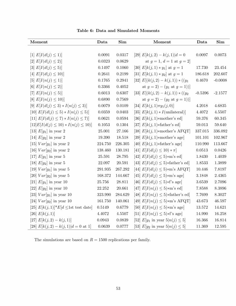
Table 6: Data and Simulated Moments

Moment Data Sim Moment Data Sim

[1] E[I(d(j) � 1)] 0.0091 0.0317 [29] E[k(j; 2)� k(j; 1)jd = 0 0.0097 0.0073

[2] E[I(d(j) � 2)] 0.0323 0.0629 at g = 1; d = 1 at g = 2]

[3] E[I(d(j) � 5)] 0.1497 0.1060 [30] E[k(j; 1) � y1] at g = 1 17.730 23.454

[4] E[I(d(j) � 10)] 0.2641 0.2199 [31] E[k(j; 1) � y2] at g = 1 186.618 202.607

[5] E[I(n(j) � 1)] 0.1765 0.2941 [32] E[(k(j; 2)� k(j; 1)) � ((y1 0.4670 -0.0008

[6] E[I(n(j) � 2)] 0.3366 0.4052 at g = 2)� (y1 at g = 1))][7] E[I(n(j) � 5)] 0.6013 0.6307 [33] E[(k(j; 2)� k(j; 1)) � ((y2 -0.5396 -2.1577

[8] E[I(n(j) � 10)] 0.6890 0.7569 at g = 2)� (y2 at g = 1))][9] E[I(d(j) � 3) � I(n(j) � 3)] 0.0079 0.0109 [34] E[k(j; 1)�y1(j; 0)] 4.2018 4.6835

[10] E[I(d(j) � 5) � I(n(j) � 5)] 0.0359 0.0403 [35] E[k(j; 1) � I(unilateral)] 4.4072 4.5507

[11] E[I(d(j) � 7) � I(n(j) � 7)] 0.0621 0.0594 [36] E[k(j; 1)�mother�s ed] 59.376 60.345

[12]E[I(d(j) � 10) � I(n(j) � 10)] 0.1053 0.1304 [37] E[k(j; 1)�father�s ed] 59.013 59.640

[13] E[y1] in year 2 25.001 27.166 [38] E[k(j; 1)�mother�s AFQT] 337.015 336.092

[14] E[y2] in year 2 19.390 18.518 [39] E[k(j; 1)�mother�s age] 101.101 102.967

[15] V ar[y1] in year 2 224.750 226.305 [40] E[k(j; 1)�father�s age] 110.990 113.667

[16] V ar[y2] in year 2 138.460 130.181 [41] E[I(d(j) � 10) � �] 0.0513 0.0426

[17] E[y1] in year 5 25.591 28.795 [42] E[I(d(j) � 5)�m�s ed] 1.8430 1.4039

[18] E[y2] in year 5 22.097 20.591 [43] E[I(d(j) � 5)�father�s ed] 1.8533 1.3899

[19] V ar[y1] in year 5 291.935 267.292 [44] E[I(d(j) � 5)�m�s AFQT] 10.446 7.8197

[20] V ar[y2] in year 5 168.372 144.667 [45] E[I(d(j) � 5)�m�s age] 3.1848 2.4365

[21] E[y1] in year 10 25.756 28.811 [46] E[I(d(j) � 5)�f�s age] 3.6539 2.7096

[22] E[y2] in year 10 22.252 20.661 [47] E[I(n(j) � 5)�m�s ed] 7.8588 8.3896

[23] V ar[y1] in year 10 323.990 284.629 [48] E[I(n(j) � 5)�father�s ed] 7.7699 8.3027

[24] V ar[y2] in year 10 161.750 140.061 [49] E[I(n(j) � 5)�m�s AFQT] 43.673 46.597

[25] E[k(j; 1)]*E[d �1st test date] 0.5149 0.6779 [50] E[I(n(j) � 5)�m�s age] 13.572 14.621

[26] E[k(j; 1)] 4.4072 4.5507 [51] E[I(n(j) � 5)�f�s age] 14.990 16.258

[27] E[k(j; 2)� k(j; 1)] 0.0943 0.0839 [52] E[y1 in year 5jn(j) � 5] 16.366 16.814

[28] E[k(j; 2)� k(j; 1)jd = 0 at 1] 0.0639 0.0777 [53] E[y2 in year 5jn(j) � 5] 11.369 12.595

The simulations are based on R = 1500 replications per family.

53

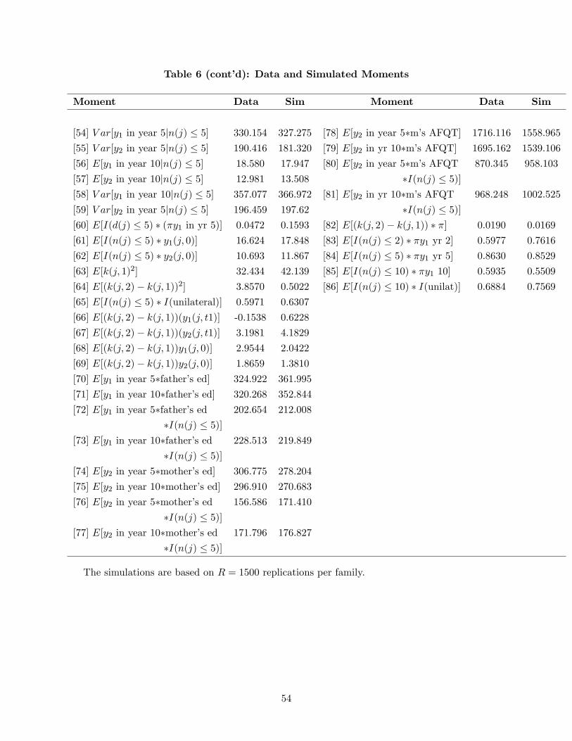
Table 6 (cont�d): Data and Simulated Moments

Moment Data Sim Moment Data Sim

[54] V ar[y1 in year 5jn(j) � 5] 330.154 327.275 [78] E[y2 in year 5�m�s AFQT] 1716.116 1558.965

[55] V ar[y2 in year 5jn(j) � 5] 190.416 181.320 [79] E[y2 in yr 10�m�s AFQT] 1695.162 1539.106

[56] E[y1 in year 10jn(j) � 5] 18.580 17.947 [80] E[y2 in year 5�m�s AFQT 870.345 958.103

[57] E[y2 in year 10jn(j) � 5] 12.981 13.508 �I(n(j) � 5)][58] V ar[y1 in year 10jn(j) � 5] 357.077 366.972 [81] E[y2 in yr 10�m�s AFQT 968.248 1002.525

[59] V ar[y2 in year 5jn(j) � 5] 196.459 197.62 �I(n(j) � 5)][60] E[I(d(j) � 5) � (�y1 in yr 5)] 0.0472 0.1593 [82] E[(k(j; 2)� k(j; 1)) � �] 0.0190 0.0169

[61] E[I(n(j) � 5) � y1(j; 0)] 16.624 17.848 [83] E[I(n(j) � 2) � �y1 yr 2] 0.5977 0.7616

[62] E[I(n(j) � 5) � y2(j; 0)] 10.693 11.867 [84] E[I(n(j) � 5) � �y1 yr 5] 0.8630 0.8529

[63] E[k(j; 1)2] 32.434 42.139 [85] E[I(n(j) � 10) � �y1 10] 0.5935 0.5509

[64] E[(k(j; 2)� k(j; 1))2] 3.8570 0.5022 [86] E[I(n(j) � 10) � I(unilat)] 0.6884 0.7569

[65] E[I(n(j) � 5) � I(unilateral)] 0.5971 0.6307

[66] E[(k(j; 2)� k(j; 1))(y1(j; t1)] -0.1538 0.6228

[67] E[(k(j; 2)� k(j; 1))(y2(j; t1)] 3.1981 4.1829

[68] E[(k(j; 2)� k(j; 1))y1(j; 0)] 2.9544 2.0422

[69] E[(k(j; 2)� k(j; 1))y2(j; 0)] 1.8659 1.3810

[70] E[y1 in year 5�father�s ed] 324.922 361.995

[71] E[y1 in year 10�father�s ed] 320.268 352.844

[72] E[y1 in year 5�father�s ed 202.654 212.008

�I(n(j) � 5)][73] E[y1 in year 10�father�s ed 228.513 219.849

�I(n(j) � 5)][74] E[y2 in year 5�mother�s ed] 306.775 278.204

[75] E[y2 in year 10�mother�s ed] 296.910 270.683

[76] E[y2 in year 5�mother�s ed 156.586 171.410

�I(n(j) � 5)][77] E[y2 in year 10�mother�s ed 171.796 176.827

�I(n(j) � 5)]

The simulations are based on R = 1500 replications per family.

54

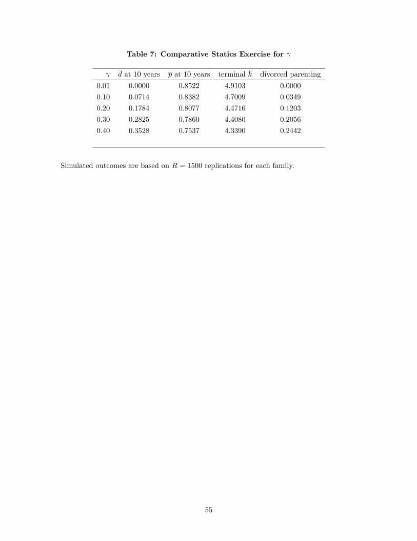
Table 7: Comparative Statics Exercise for

d at 10 years p at 10 years terminal k divorced parenting

0.01 0.0000 0.8522 4.9103 0.0000

0.10 0.0714 0.8382 4.7009 0.0349

0.20 0.1784 0.8077 4.4716 0.1203

0.30 0.2825 0.7860 4.4080 0.2056

0.40 0.3528 0.7537 4.3390 0.2442

Simulated outcomes are based on R = 1500 replications for each family.

55

Table 8: Comparative Statics Exercise for Custody

�1(1) d at 10 years p at 10 years terminal k divorced parenting

0.00 0.1065 0.7022 4.4873 0.0957

0.10 0.1785 0.7626 4.8909 0.1132

0.20 0.2199 0.7569 4.6346 0.1304

0.30 0.2575 0.7270 4.7384 0.1336

0.40 0.2259 0.8065 4.8189 0.1387

0.50 0.2350 0.8987 5.6185 0.1630

Simulated outcomes are based on R = 1500 replications for each family.

56

Table 9: Comparative Statics Exercises for Child Support

� d at 10 years p at 10 years terminal k divorced parenting

0.00 0.2114 0.7702 4.5556 0.1303

0.10 0.2196 0.7796 4.6132 0.1315

0.17 0.2138 0.7669 4.5589 0.1333

0.20 0.2137 0.7695 4.6008 0.1274

0.25 0.1985 0.7658 4.7126 0.1288

0.30 0.1973 0.7643 4.6935 0.1291

Simulated outcomes are based on R = 1500 replications for each family.

57

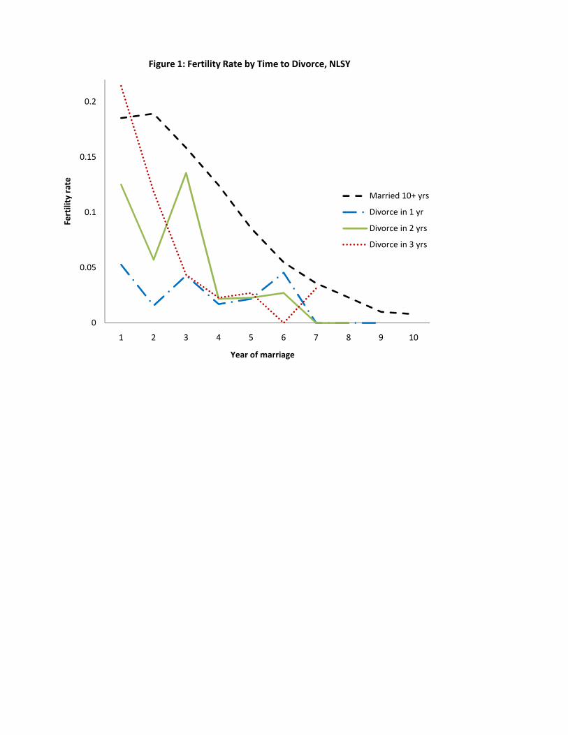
0

0.05

0.1

0.15

0.2

1 2 3 4 5 6 7 8 9 10

Fertility rate

Year of marriage

Figure 1: Fertility Rate by Time to Divorce, NLSY

Married 10+ yrs

Divorce in 1 yr

Divorce in 2 yrs

Divorce in 3 yrs

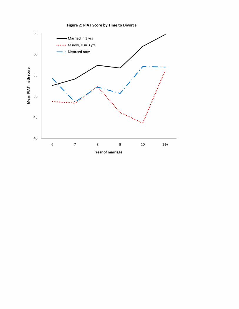
60

65

Figure 2: PIAT Score by Time to Divorce

Married in 3 yrs

M now, D in 3 yrs

Divorced now

55

60

65PIAT math score

Figure 2: PIAT Score by Time to Divorce

Married in 3 yrs

M now, D in 3 yrs

Divorced now

45

50

55

60

65Mean PIAT math score

Figure 2: PIAT Score by Time to Divorce

Married in 3 yrs

M now, D in 3 yrs

Divorced now

40

45

50

55

60

65

6 7 8 9 10 11+

Mean PIAT math score

Year of marriage

Figure 2: PIAT Score by Time to Divorce

Married in 3 yrs

M now, D in 3 yrs

Divorced now

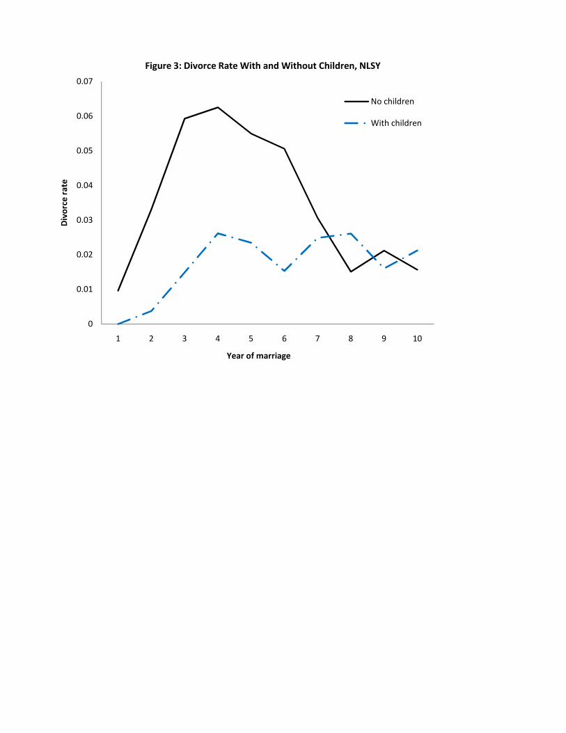
0

0.01

0.02

0.03

0.04

0.05

0.06

0.07

1 2 3 4 5 6 7 8 9 10

Divorce rate

Year of marriage

Figure 3: Divorce Rate With and Without Children, NLSY

No children

With children

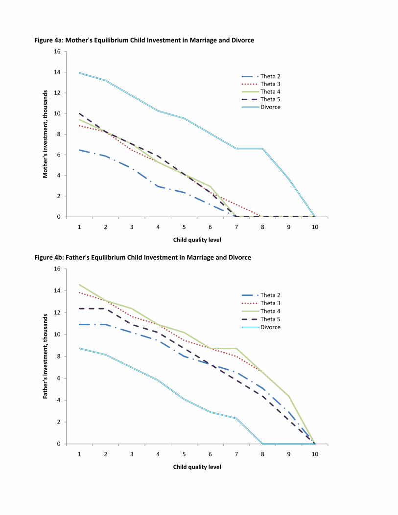
Figure 4a: Mother's Equilibrium Child Investment in Marriage and Divorce

Figure 4b: Father's Equilibrium Child Investment in Marriage and Divorce

16

0

2

4

6

8

10

12

14

16

1 2 3 4 5 6 7 8 9 10

Mothe

r's investmen

t, tho

usan

ds

Child quality level

Theta 2Theta 3Theta 4Theta 5Divorce

0

2

4

6

8

10

12

14

16

1 2 3 4 5 6 7 8 9 10

Father's investmen

t, tho

usan

ds

Child quality level

Theta 2Theta 3Theta 4Theta 5Divorce

0

2

4

6

8

10

12

14

16

1 2 3 4 5 6 7 8 9 10

Mothe

r's investmen

t, tho

usan

ds

Child quality level

Theta 2Theta 3Theta 4Theta 5Divorce

Figure 5: Ex ante average welfare by paternal custody share

th no child

lue of m

arriage wit

Tau1(1) = 0.5

Tau1(1) = 0.4

Tau1(1) = 0.3

Tau1(1) = 0.2

Ex ante average va

Tau1(1)   0.2

Tau1(1) = 0.1

Tau1(1) = 0

0 0.05 0.1 0.15 0.2 0.25 0.3

Child support rate

dFigure 6: Spouses' Welfare and Child Support, 50/50 Custody

Husband's ex ante welfare

Wife's ex ante welfare

marriage with no

 child

welfare

Wife's ex ante welfare

Average ex ante welfare

Ex ante value of m

arriag

0 0.05 0.1 0.15 0.2 0.25 0.30 0.05 0.1 0.15 0.2 0.25 0.3

Child support rate