The Effect of Fertility Reduction on Economic Growth∗

Quamrul H. Ashraf† David N. Weil‡ Joshua Wilde§

October 2012

Abstract

We assess quantitatively the effect of exogenous reductions in fertility on output per

capita. Our simulation model allows for effects that run through schooling, the size

and age structure of the population, capital accumulation, parental time input into

child-rearing, and crowding of fixed natural resources. The model is parameterized

using a combination of microeconomic estimates, data on demographics and natural

resource income in developing countries, and standard components of quantitative

macroeconomic theory. We apply the model to examine the effect of a change in

fertility from the UN medium-variant to the UN low-variant projection, using Nigerian

vital rates as a baseline. For a base case set of parameters, we find that such a change

would raise output per capita by 5.6 percent at a horizon of 20 years, and by 11.9

percent at a horizon of 50 years.

Keywords: Fertility, Population size, Age structure, Child quality, Worker experience,

Labor force participation, Capital accumulation, Natural resources, Income per capita

JEL Codes: E17, J11, J13, J18, J21, J22, J24, O11, O13, O55

∗We thank Günther Fink, Andrew Foster, Stelios Michalopoulos, Alexia Prskawetz, and participants

at Bar-Ilan Univeristy, the 2010 NEUDC Conference, the IUSSP Seminar on “Demographics and

Macroeconomic Performance,”Paris, 2010, the 4th Annual “PopPov”Research Conference on “Population,

Reproductive Health, and Economic Development,”Cape Town, 2010, and the conference, “China and the

West 1950—2050: Economic Growth, Demographic Transition and Pensions,”University of Zurich, 2011, for

comments, and Daniel Prinz for research assistance. Financial support from the William and Flora Hewlett

Foundation and the MacArthur Foundation is gratefully acknowledged.

†Williams College and Harvard Kennedy School.‡Brown University and NBER.§University of South Florida.

1 Introduction

How does population growth affect economic growth? More concretely, in the context of a

high-fertility developing country, how much higher would income per capita be if the fertility

rate were to fall by a specified amount? This is an old question in economics, going back

at least to Malthus (1798). Over the last half century, the consensus view has shifted from

fertility declines having strong effects, to their not being very important, and recently back

toward assigning them some significance (Sindig 2009; Das Gupta, Bongaarts, and Cleland

2011).

For an issue that has been studied for so long, and with such potential import,

the base of evidence regarding the economic effects of fertility (or population growth more

generally) is rather weak. In some ways, this should not be a surprise. Population growth

changes endogenously as a country develops. Further, factors that impact population, such

as changes in institutions or culture, are also likely to affect economic growth directly, and

they are poorly observed as well. Finally, the lags at which fertility changes affect economic

outcomes may be fairly long. Thus, at the macroeconomic level, it is very hard to sort out

the direct effects of population growth from those of other factors. Much of the current

thinking about the aggregate effects of fertility decline relies on results from cross-country

regressions in which the dependent variable is growth of GDP per capita and the independent

variables include measures of fertility and mortality, or else measures of the age structure of

the population. However, as discussed in Section 2, there are severe econometric problems

with this approach.

Our goal in this paper is to quantitatively analyze the economic effects of reductions

in fertility in a developing country where initial fertility is high. We ask how economic

measures such as GDP per capita would compare in the case where some exogenous change

reduces fertility to the case where no such exogenous change takes place. The answer to

this question will be very different from simply observing the natural coevolution of fertility

and economic development, because in our thought experiment we hold constant all the

unobserved factors that in reality affect both fertility and economic growth.

To address our research question, we construct an demographic-economic simulation

model in which fertility can be exogenously varied.1 We trace out the paths of economic

development under two scenarios: a “baseline,” in which fertility follows a specified time

path, and an “alternative”in which fertility is lower. Because we want to realistically model

high-fertility developing countries in which fertility will likely be falling over the next several

1A fully functioning version of the model, which the user can manipulate to shut down channels, changeparameters, and alter the demographic scenario, is available from the authors upon request.

1

decades, both our baseline and alternative scenarios involve falling paths of fertility; the

difference is that fertility falls faster in the alternative scenario. We use the United Nations

(UN 2010) medium-fertility population projection as our baseline, and the UN low-fertility

population projection as our alternative scenario.2

The model we build takes proper account of general equilibrium effects, the dynamic

evolution of population age structure, accumulation of physical and human capital, and

resource congestion. It is parameterized using a combination of microeconomic evidence and

economic theory. Throughout the paper, our focus is on giving a quantitative analysis of

changes in fertility, so that we can estimate how much extra output a given fertility change

will produce over a specific time period. The simulation approach also permits an analysis of

the strength of the various mechanisms at work. We hope that, by showing how behavioral

effects that are often studied in isolation can be integrated to answer macroeconomic ques-

tions, we can reorient the academic discussion of population and development along more

quantitative and practical lines.

The methodology we employ is not conceptually new. Rather, we are proceeding

in the tradition of Coale and Hoover (1958) and many others discussed below. However,

we improve on existing work in several dimensions. First, we trace out the effects of

changes in the population through many more potential channels than were addressed in

previous literature.3 Second, we ground our estimates of the magnitudes of effects in well-

identified microeconomic studies of individual behavior. In much of the previous literature,

key magnitudes were chosen either in an ad hoc fashion or solely based on theory. Third, we

are able to measure the magnitude of the different channels that are analyzed. This makes

the simulation rather less of a black box. Finally, the structure of our simulation is both

transparent and flexible. The paper itself includes a good deal of robustness testing, and

our full computer model is available and easily altered by anyone wishing to conduct further

testing. The simulation model that we build is general, but it has characteristics that can be

tailored to the situation of particular countries. In addition to country-specific demographic

2An earlier version of this paper, with a slightly different title —“The Effect of Interventions to ReduceFertility on Economic Growth,”featured a baseline scenario of constant fertility (in a stable population) andan alternative scenario of the total fertility rate falling instantaneously by one and then remaining at thatlevel indefinitely. While far less realistic, this setup allowed for a cleaner analysis of the time profiles withwhich different channels leading from fertility to economic outcomes operate. That paper is available uponrequest.

3Our analysis in this paper is focused on developing countries, and thus the particular economic channelsthat we consider in our model are those that we think are most germane in this context. For more developedcountries, which have lower population growth, older population age structures, and large government-mediated transfers to the elderly, different issues are relevant. See, for example, Weil (2008b) and Colemanand Rowthorn (2011).

2

characteristics (vital rates, initial age structure), the model can incorporate country-specific

measures of the role of natural resources in aggregate production and the openness of the

capital market.

To reiterate a point made above, our goal in this paper is not to build the best

possible forecast of the actual path of GDP per capita in a particular country. Rather, our

interest is in asking how the forecast path of GDP would change in response to a change in

fertility. That is, we compare the paths of GDP in two otherwise identical scenarios that

differ only in terms of fertility. Such an exercise necessitates a baseline scenario from which

to work. We use a very straightforward baseline in which, for example, productivity growth

is constant. While one could consider a different baseline, it is important to note that errors

in the baseline forecast that we use will only have second-order effects on our estimate of the

difference between the baseline and alternative scenarios.

Our finding is that a reduction in fertility raises income per capita by an amount

that some would consider economically significant, although the effect is small relative to

the vast gaps in income between developed and developing countries. In the version of

our model parameterized to match the economic and demographic situation of Nigeria, we

find that shifting from the UN medium-fertility population projection to the UN low-fertility

population projection raises income per capita by 5.6 percent at a horizon of 20 years, and by

11.9 percent at a horizon of 50 years. The simple dependency effect (fewer dependent children

relative to working adults) is the dominant channel for the first several decades. At longer

horizons, the effects of congestion of fixed resources (à la Malthus) and capital shallowing (à

la Solow) become more significant than dependency, although the latter remains important.

The fourth most important channel in the long run is the increase in human capital that

follows from reduced fertility.

Whether the overall effect of fertility on economic outcomes that we find in our model

is large or small is mostly in the eye of the beholder —a point to which we return in the

paper’s conclusion. It is also important to note the hurdles that stand between a finding that

reductions in fertility would raise output per capita by an economically significant amount

(if that is how one interprets the magnitude of our finding) and a conclusion that some

policy intervention that achieved such a reduction in fertility would be a good thing. First,

our analysis says nothing at all about the methods, costs, or welfare implications of such

interventions. Second, GDP per capita is not necessarily the correct welfare criterion. The

question of how a social planner should treat the welfare of people who may not be born as

a result of some policy is notoriously diffi cult (Razin and Sadka 1995; Golosov, Jones, and

Tertilt 2007).

3

The rest of this paper is structured as follows. Section 2 discusses how our work

relates to the previous literature. Section 3 discusses the baseline and alternative fertility

scenarios we consider and shows how the dynamic paths of population size and age structure

differ between them. Section 4 presents the economic model and discusses our choice of base

case parameters. Section 5 presents simulation results for the base case model, discusses the

sensitivity of results to altering our parameter assumptions, and presents a decomposition

of the effects of fertility on output via different channels. Section 6 looks more deeply at

different choices regarding the investment rate and how they interact with demographic

change. Section 7 similarly goes into greater depth regarding assumptions about the role of

the fixed factor in production. Section 8 concludes.

2 Relationship to previous literature

Attempts to assess the effect of fertility changes on economic outcomes can be classified

among three categories: aggregate (macroeconomic) statistical analyses, microeconomic

studies, and simulation modeling. In this section, we briefly review these three approaches,

and we also discuss a number of studies that have presented broad syntheses of research on

the topic. Of course, the existing literature is vast in all of these areas, and so our summary

is by necessity highly selective. We conclude the section by discussing how the approach we

take in the rest of the paper compares to what has come before.

2.1 Macroeconomic analyses

The best known early aggregate analysis of the relationship between population growth and

development is Kuznets (1967). His study found a positive correlation between growth rates

of population and income per capita within broad country groupings, which he interpreted

as evidence of a lack of a negative causal effect of population growth on income growth,

contrary to the prevailing view at the time.

A number of studies followed in the line of Kuznets (1967) in examining the relation-

ship between population growth and different factors that were viewed as being determinants

of income growth. For example, Kelley (1988) found no correlation between population

growth and growth of income per capita, and similarly no relationship between population

growth and saving rates. Summarizing many other studies, he concluded that the evidence

documenting a negative effect of population growth on economic development was “weak or

nonexistent.”

4

Since the early 1990s, many analyses of the effect of population on economic outcomes

have followed the “growth regression” model popularized by Barro (1991) and Mankiw,

Romer, and Weil (1992). In these regressions, terms representing population growth, labor

force growth, or dependency ratios are included as right hand side variables. For example,

Kelley and Schmidt (2005) regress the growth rate of income per capita on the growth rates of

total population and the working-age population, incorporating both Solow effects (dilution

of the capital stock by rapid growth in the number of workers) and dependency effects.

They find that the demographic terms are quantitatively important. More specifically, their

regression explains approximately 20 percent of the growth of income per capita on average

over the period 1960—1995. Bloom and Canning (2008) regress the growth rate of income per

capita on the growth rate of the working-age fraction of the population (along with standard

controls), finding a positive and significant coeffi cient. Since high growth of the working-age

fraction follows mechanically from fertility reductions, they see this as showing the economic

benefits of reduced fertility.

Unfortunately, very little of the literature taking an aggregate approach to the effects

of population on economic outcomes deals adequately with the issue of identification. The

determinants of population growth, most notably fertility, are endogenous variables. Changes

in fertility are not only themselves affected by economic outcomes, but they are also affected

by unobserved variables that may also have direct effects on the economy. These could

include human capital, health, characteristics of institutions, cultural outlook, and so on.

Because of these issues of omitted variables and reverse causation, the ability to draw

inferences from the conditional correlations in growth regressions is very weak.4 The fact

that changes in economic outcomes are sometimes regressed on lagged changes in fertility

(as represented, for example, by population age structure) is only a slight improvement, since

there is bound to be serial correlation in the unobserved factors that affect both fertility and

economic outcomes.

A small number of studies have attempted to circumvent the identification problem

in the macroeconomic context using instrumental variables. Acemoglu and Johnson (2007),

using worldwide health improvements during the international epidemiological transition

to instrument for country-specific reductions in mortality, conclude that higher population

growth has a significant negative effect on GDP per capita at a horizon of several decades.

Li and Zhang (2007) use shares of non-Han populations (which were not subject to the one-

child policy) across Chinese provinces to instrument for population growth, finding a negative

effect on the growth of GDP per capita. Bloom et al. (2009), using abortion legislation as

4See Deaton (1999) for a critique.

5

an instrument, find a negative impact of fertility on female labor force participation. They

conclude that the extra labor supply would be a significant channel through which lower

fertility would raise income growth, although they mention that saving and human capital

accumulation are expected to be important channels as well.

2.2 Microeconomic analyses

A second approach to examining the relationship between population and economic outcomes

has been to look to a finer level of analysis: households, rather than countries. Examination

of household data often allows for proper identification to be achieved in a way in which

it cannot be done using macro data. Joshi and Schultz (2007) and Schultz (2009) study

the long run effects of a randomized trial of contraception provision in Matlab, Bangladesh.

They find that reduced fertility produced persistent and significant positive effects on the

health, earnings, and household assets of women, and on the health and earnings of children.

Miller (2010) uses variations in the timing of the introduction of the Profamilia program

in Colombia to identify both the effect of contraceptive availability on fertility and the

effect of fertility on social and economic outcomes. He finds that ability to postpone first

births leads to higher education as well as independence for women. For those treated at a

young age, Profamilia reduced fertility by 11-12 percent and raised education by 0.08 years.

Rosenzweig and Zhang (2009), examining data from China and using twins as a source of

exogenous variation in the number of children, find that higher fertility reduces educational

attainment. For rural areas, the elasticity of schooling progress with respect to family size is

estimated at between -9 and -26 percent. On the other hand, Angrist, Lavy, and Schlosser

(2006) in Israeli data, and Black, Devereux, and Salvanes (2005) in Norwegian data, using

twins as well as sex-mix preference as instruments for the number of children, find no effect

of the number of children on child quality.

While cross-country regressions suffer from severe econometric problems, they do have

the advantage —if one is interested in studying the aggregate effects of fertility decline —of

focusing on the right dependent variable. By contrast, a good many microeconomic studies

examine the link between fertility at the household level and various outcomes for individuals

in that household (wages, labor force participation, education, etc.). These studies cannot

directly answer the question of how fertility reduction affects the aggregate economy for three

reasons. First, many of the effects of such reduction run through channels external to the

household —either via externalities in the classic economic sense (for example, environmental

degradation) or through changes in market prices, such as wages, land rents, and returns to

capital (Acemoglu 2010). Second, even if one ignores the issue of external effects, aggregating

6

the different channels by which fertility affects economic outcomes is not trivial. Finally, as

in the macroeconomic literature, the long time horizon over which the effects of fertility

change will affect the economy limits the ability of a single study to capture them.

2.3 Simulation models

In principle, if one knows the magnitude of the different structural channels that relate

economic and demographic variables, these can be combined into a single simulation that

will effectively deal with the issues of aggregation and general equilibrium. In practice,

however, simulation models are only as credible as their individual components —that is,

both the structural channels that they incorporate and the manner in which these structural

relationships are parameterized.

The intellectual ancestor of modern economic-demographic models is Coale and Hoover

(1958), who set out to study the effect of fertility change in India. They start by making

alternative population forecasts for India under three exogenous fertility scenarios: high

(constant at its 1951 level), medium (declining 50 percent over the period 1966—1981), and

low (declining 50 percent over the period 1956—1981). Total population in 1986 in their model

is 22 percent higher in the high-fertility than the medium-fertility scenario, and 7 percent

lower in the low-fertility than the medium-fertility scenario. In terms of production, the

authors assume that there is an exogenous incremental capital-output ratio that is invariant

to investment and population (there is no human capital or land in the production function).

Their finding is that, at a time horizon of 30 years, income per capita is 15 percent higher

in the low-fertility scenario and 23 percent lower in the high-fertility scenario as compared

to the medium-fertility scenario. The primary mechanism driving their results is capital

accumulation: with high population growth, a high dependency ratio negatively impacts the

saving rate and thus investment and growth. Of particular note, the model treats spending

on child health and education as consumption rather than investment.

A recognizably more modern production model is incorporated into Denton and

Spencer (1973). They use a neoclassical production function that allows the marginal

products of capital and labor to vary with the capital-labor ratio. Fertility and mortality

rates are taken as exogenous. The model includes capital accumulation (with saving being

a fixed fraction of disposable income) and age-specific labor supply. The model is fit to

data from Canada and is used to analyze the aggregate effects of changes in the fertility

path. Enke (1971) applies a somewhat similar model to a stylized developing country. He

compares paths of income per capita under two scenarios: a high-fertility scenario, in which

the gross reproduction rate (GRR) stays constant at 3.025 from 1970 through 2000, and a

7

low-fertility scenario in which the GRR falls from 3.025 in 1970 to 2.09 in 1985 and 1.48

in 2000. Total population in 2000 is 37 percent higher in the high-fertility than in the

low-fertility scenario. The underlying economic model uses capital and labor as inputs in a

Cobb-Douglas production function.5 Population is divided into 5-year intervals, with varying

age-specific labor force participation. The effects that he finds are quite large: income per

capita in the low-fertility scenario is 13 percent larger than in the high-fertility scenario

in 1985, and it is 43 percent larger in 2000. Much of the force driving his results comes

from a higher saving rate in the low-fertility scenario that is, in turn, due to a Keynesian

consumption function in which the average propensity to consume falls as disposable income

rises, and in which the level of consumption is partially proportional to population size.

Simon’s (1976) model is similar in many respects to that of Enke (1971), but with

several alterations that reverse key results. In Simon (1976), social overhead capital rises

with population size to allow for economies of scale in production (specifically, better road

networks that facilitate more effi cient production). Similarly, technological change in the

industrial sector is a function of the overall size of the population. Unlike Enke (1971),

the model also features an explicit labor-leisure choice as well as separate agricultural and

industrial sectors. Taking fertility as exogenous, Simon (1976) finds that, for the first 60

years of the simulation, constant population size leads to higher income per capita than

growing population, although the difference is quite small. For longer time horizons, growing

population (at a moderate rate) is better than constant population.

Simulation models that developed further in this line included multiple productive

sectors (agriculture, industrial, and service), a government sector, and urbanization. Several

also included an endogenous response of fertility. In reviewing a number of these models,

Ahlburg (1987) argues that they “vary considerably in their complexity... The cost of the

models’ increased complexity is that it is often very diffi cult to uncover the underlying

assumptions and, particularly, since few carry out sensitivity analysis, the key assumptions.”

His summary of the concrete findings of these simulation models is that fertility decline would

have modest positive effects on income per capita, although much smaller than predicted by

population pessimists such as Enke (1971).

In a similar vein, Kelley (1988) cites many obstacles to constructing a credible model

to address the issue of how rapid population growth impacts development in the ThirdWorld.

Among these obstacles are general equilibrium feedbacks, the diffi culty of constructing

credible long-range demographic forecasts, potential changes in policy or institutions that

5The exponents on capital and labor are 0.4 and 0.5, respectively, implying a 10 percent share for a fixedfactor (presumably land).

8

may occur over the forecast interval, and the lack of available data to specify and validate

such a model. He concludes, “Clearly, providing a quantitative, net-economic-impact answer

to the population-counterfactual question is at best a remote possibility.”

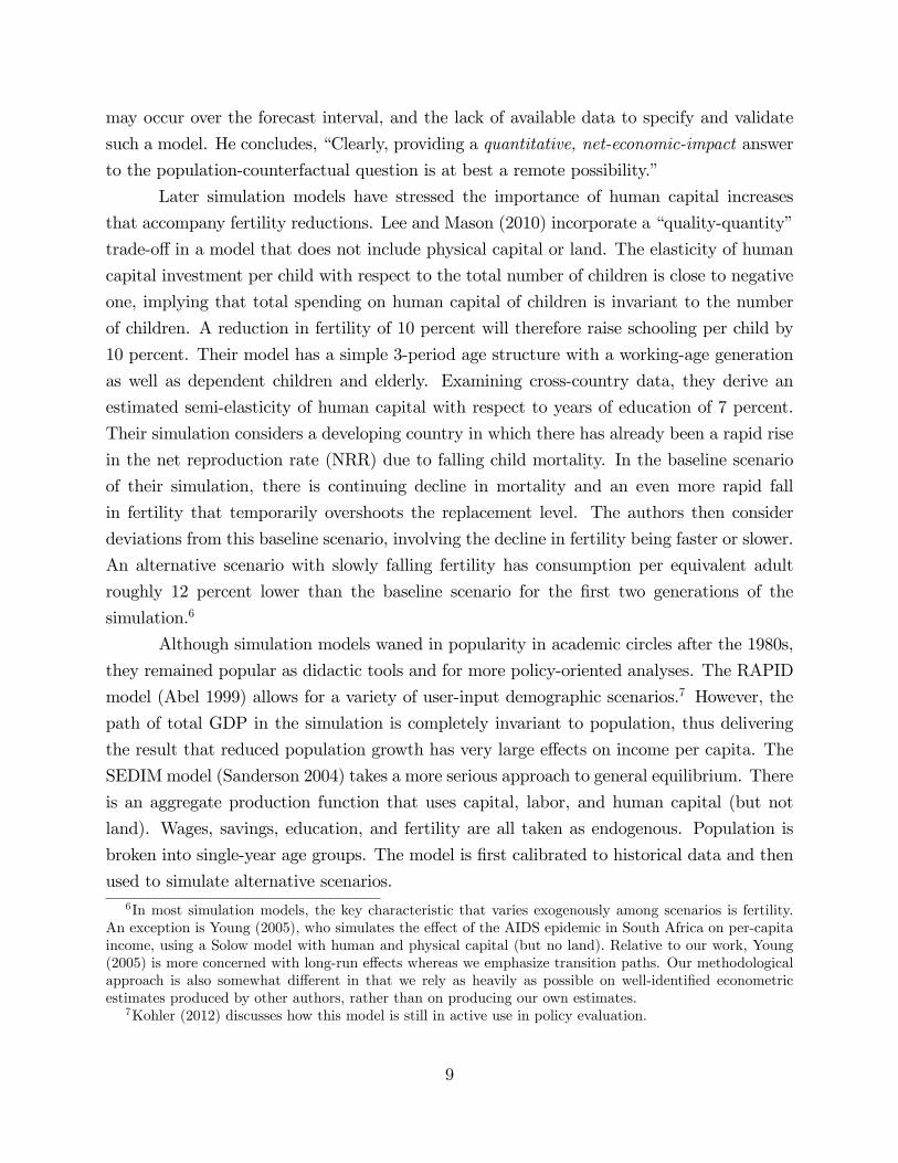
Later simulation models have stressed the importance of human capital increases

that accompany fertility reductions. Lee and Mason (2010) incorporate a “quality-quantity”

trade-off in a model that does not include physical capital or land. The elasticity of human

capital investment per child with respect to the total number of children is close to negative

one, implying that total spending on human capital of children is invariant to the number

of children. A reduction in fertility of 10 percent will therefore raise schooling per child by

10 percent. Their model has a simple 3-period age structure with a working-age generation

as well as dependent children and elderly. Examining cross-country data, they derive an

estimated semi-elasticity of human capital with respect to years of education of 7 percent.

Their simulation considers a developing country in which there has already been a rapid rise

in the net reproduction rate (NRR) due to falling child mortality. In the baseline scenario

of their simulation, there is continuing decline in mortality and an even more rapid fall

in fertility that temporarily overshoots the replacement level. The authors then consider

deviations from this baseline scenario, involving the decline in fertility being faster or slower.

An alternative scenario with slowly falling fertility has consumption per equivalent adult

roughly 12 percent lower than the baseline scenario for the first two generations of the

simulation.6

Although simulation models waned in popularity in academic circles after the 1980s,

they remained popular as didactic tools and for more policy-oriented analyses. The RAPID

model (Abel 1999) allows for a variety of user-input demographic scenarios.7 However, the

path of total GDP in the simulation is completely invariant to population, thus delivering

the result that reduced population growth has very large effects on income per capita. The

SEDIMmodel (Sanderson 2004) takes a more serious approach to general equilibrium. There

is an aggregate production function that uses capital, labor, and human capital (but not

land). Wages, savings, education, and fertility are all taken as endogenous. Population is

broken into single-year age groups. The model is first calibrated to historical data and then

used to simulate alternative scenarios.6In most simulation models, the key characteristic that varies exogenously among scenarios is fertility.

An exception is Young (2005), who simulates the effect of the AIDS epidemic in South Africa on per-capitaincome, using a Solow model with human and physical capital (but no land). Relative to our work, Young(2005) is more concerned with long-run effects whereas we emphasize transition paths. Our methodologicalapproach is also somewhat different in that we rely as heavily as possible on well-identified econometricestimates produced by other authors, rather than on producing our own estimates.

7Kohler (2012) discusses how this model is still in active use in policy evaluation.

9

In many of the models discussed above, one of the crucial channels through which

demographic change affects economic outcomes is saving and capital accumulation. An issue

that any such model must deal with is whether and how the consumption/saving decisions

made by households are affected by their expectations of future demographic and economic

developments. In modern macroeconomic models, the standard assumption is of rational

or model-consistent expectations, although application of this assumption in the case of

long-run demographic change can be quite complex. Auerbach and Kotlikoff’s (1987) 55-

period overlapping generations model represents a methodology for solving for the rational

expectations equilibrium in such a case, although their emphasis is on developed-country

issues, in particular government funded transfer programs.

Recent work by macroeconomists interested in long-run growth has extended the

approach of Auerbach and Kotlikoff (1987) to create fully “micro-founded” computable

general equilibrium models to analyze the interaction of population and economic outcomes

(for example, Doepke, Hazan, and Maoz 2007). In such work, utility maximizing house-

holds are modeled as continuously reoptimizing their decisions (fertility, child education,

consumption, labor supply) in response to changes in forecast paths of aggregate variables.

The approach requires explicitly modeling household utility functions, including preferences

over child quality and quantity, as well as budget constraints and credit market constraints

faced by households and firms.

2.4 Broad syntheses

Two of the most important syntheses of contemporary thinking on the subject of how

fertility affects development in poor countries are those by the National Academy of Sciences

(NAS 1971) and the National Research Council (NRC 1986). NAS (1971) presents nuanced

discussions of many of the potential channels through which rapid population growth can

affect economic outcomes, including resource depletion, capital dilution due to rapid labor

force growth, urbanization, and reductions in the saving rate caused by a large dependent

population. In contrast to much of the literature up to the time, there is a strong emphasis

on the role of human capital, and the increase in the fraction of national income that must

be devoted to education when fertility is high. The authors are circumspect regarding

the diffi culties of long-range forecasting. They mostly limit themselves to a horizon of 2-3

decades, during which the dominant effects of fertility changes will be on the numbers of

dependent children, and comment on the lack of credible models with which to make longer-

term assessments. Although they firmly eschew the idea of a “population crisis” that was

popular at the time, they nevertheless conclude that lower population growth in developing

10

countries would significantly increase income per capita, and that reduced fertility should

be a policy goal for most developing nations. Specifically, they urge countries with high

population growth to reduce their rates of natural increase to less than 15 per 1,000 over the

following two decades.

NRC (1986) is most notable for crystallizing a perspective skeptical of theorized neg-

ative effects of population growth, based both on available empirical evidence and principles

of economic theory. The report also stresses the economic mechanisms that work to reduce

negative effects of population growth, in particular the ability of markets and institutions

to adjust to increased population. Much of the intellectual heft of the report is directed at

the question of whether interventions in fertility decisions of households are warranted. The

authors focus in particular on the questions of externalities and imperfect information on the

part of households. To the extent that couples take into account the effect of their fertility

decisions on the health and economic success of their children (including, for example, the

effect of lower fertility on education and land per capita), the authors do not see a role

for government. To an even greater extent than NAS (1971), the authors of NRC (1986)

are reluctant to take a quantitative approach to discussing the effects of fertility change on

long-term economic outcomes.8

NRC (1986) is often identified as the standard-bearer of the “revisionist”view that

fertility change has a relatively small effect on economic development. Over the last decade,

however, the pendulum has swung somewhat back in the other direction. Kohler (2012)

starts by pointing out that although the majority of the world’s population now lives in

countries where fertility has fallen below the replacement rate, there are substantial areas

of the world in which fertility remains quite high —specifically, with an NRR above 1.5 and

a growth rate of population above 2.5 percent per year. Regarding these areas, he assesses

the degree to which continued high fertility or stalled fertility declines constitute threats to

economic development (as part of a broader cost-benefit evaluation of policies targeted at

reducing population growth). He pays particular attention to the views of a new generation

of population pessimists, typified by Campbell et al. (2007). Kohler’s (2012) review of

the different channels by which population affects economic outcomes includes resource

scarcity, the “demographic dividend”from changes in population age structure, and effects

of population size on innovation. His admittedly very rough and ready conclusion is that

in current high-fertility countries a reduction of one percent per year in population growth

would yield an increase of one percent per year in growth of income per capita. Another

8Birdsall (1988) and Kelley (1988) are excellent summaries of contemporary thinking about the effect offertility on economic outcomes.

11

recent synthesis of current research (Das Gupta, Bongaarts, and Cleland 2011) concludes

“At bottom, there is little fundamental disagreement on the issue. There is broad consensus

that policy settings that support growth are the key drivers of economic growth, while

population size and structure play an important secondary role in facilitating or hindering

economic growth.”Sindig (2009) also reviews the current literature, identifying an emerging

consensus that fertility reduction, while not a suffi cient condition for economic growth, may

well be a necessary one.

2.5 Structure of our model

In its basic structure, our model is clearly in the tradition of the simulation studies discussed

above. We construct a general equilibrium model in which fertility and mortality (and thus

population size and age structure) are exogenous. The endogenous variables in the model

include physical and human capital, labor force participation, and wages. Output is produced

in a neoclassical production function that takes physical capital, land, and a human capital

aggregate (embodying education and experience) as inputs. Population is divided into 5-year

age groups, and the time interval is 5 years.

An important way in which our model differs from previous work is that we focus

not only on the overall effect of fertility change, but on the different channels by which

fertility impacts the economy. This focus on channels allows for a more nuanced discussion

of how our results compare to the predictions of different theories. Existing literature has

discussed a number of channels that lead from demographic change to economic outcomes.

At the risk of some intellectual straight-jacketing, we classify these effects as follows. The

most basic effect of population on output per capita is through the congestion of fixed

factors, such as land. We call this the Malthus effect. A second channel is the capital

shallowing that results from higher growth in the labor force. We call this the Solow effect.

Four channels run through the age structure of the population, which is a function of past

fertility and mortality rates. First, in a high-fertility environment, a reduction in fertility

leads, at least temporarily, to a higher ratio of working-age adults to dependents. Holding

income per worker constant, this mechanically raises income per capita. We call this the

dependency effect. Second, a concentration of population in their working years may raise

national saving, feeding through to higher capital accumulation and higher output. We call

this the life-cycle saving effect. Work by Bloom and Williamson (1998) on the demographic

dividend has stressed a combination of the dependency and life-cycle saving effects. Third,

slower population growth shifts the age distribution of the working-age population itself

toward higher ages. In developing countries, this increase in average experience would be

12

expected to raise productivity, even though in more developed countries the shift into late

middle ages might lower productivity. We call this the experience effect. Fourth, if older

workers participate in the labor market at a higher rate than workers just entering the

workforce, the shifting age distribution towards higher ages will lead to higher overall labor

force participation, thereby increasing income per capita. We call this the life-cycle labor

supply effect. Another effect of reduced fertility is to lower the quantity of adult time that

is devoted to child-rearing, freeing up more time for productive labor. We call this the

childcare effect. Reductions in fertility are often associated with an increase in parental

investment per child. We call this the child-quality effect. Finally, an increase in the size of

the population may raise productivity directly, by allowing for economies of scale, or may

induce technological or institutional change that raises income per capita.9 We call this the

Boserup effect. In this paper, we attempt to quantify the first eight of these effects (Malthus,

Solow, dependency, life-cycle saving, experience, life-cycle labor supply, childcare, and child

quality).

A second significant difference between our model and previous simulations is in the

parameterization of the underlying economic relations. In comparison to previous studies, we

go much further in grounding our parameterization in well-identified microeconomic analyses

of the types discussed above. The channels that we parameterize in this fashion include the

returns to schooling and experience, the effect of fertility on education, and the effect of

fertility on female labor supply. The range of existing estimates and our procedures for

choosing parameters are discussed in Section 4 of the paper.

Unlike models in the tradition of Auerbach and Kotlikoff (1987), the saving and

human capital investment decisions in our model do not have any forward looking compo-

nent. Similarly, we do not provide a complete foundation for household decisions in terms

of household optimization. Rather, we look at the applied microeconomics literature for

estimates of the effects of contemporaneous variables on accumulation (such as education).

In our view, economists’s current understanding of household decision-making in developing

countries is simply too limited to produce a quantitatively useful model that incorporates a

fully optimizing micro-founded setup.

Of all the simulation models discussed above, the one that is closest in spirit to

ours is the SEDIM model. The biggest difference between SEDIM and our model is in

the calibration of key parameters. As discussed below, we rely on formal microeconomic

estimates to supply the key parameters of our model, including the effects of education and

9There may also be a direct effect of the age structure of the population on productivity. See Feyrer(2008).

13

experience on labor effi ciency, the effect of fertility on education and labor supply, and so

on. By contrast, the SEDIM model takes a much more ad hoc approach. A second difference

is that unlike the SEDIM model, we do not allow for the endogenous evolution of fertility

in response to changes in income (that result from an initial change in fertility). We are

sympathetic to this approach and may pursue it in future research, but at this point we hold

off for two reasons: first, there is no well-identified measure of how much fertility should

respond to such a change; and second, our basic analysis shows that the response of income

to fertility declines is relatively modest, and so we would expect the “second-round”effect

of income on fertility to be modest as well. Finally, the SEDIM model has no land or fixed

resources, and so the Malthusian effect of population increase is ignored.

Unlike Simon (1976), we take technological change as fully exogenous. His view that a

higher level of population will lead to more technological progress, because there will be more

people available to come up with new ideas, has been incorporated into the macro-growth

literature (see, for example, Jones 1995). However, in our view, these models are better

applied to the world as a whole or to the countries at the cutting edge of technology than

to individual developing countries for a simple reason: the vast majority of technological

progress in a typical developing country will be imported from abroad, and thus the growth

rate of technology will be insensitive to the country’s own population.

One way in which our approach differs significantly from that of NRC (1986) is that

we explicitly focus on output per capita rather than utility. The question of how properly-

considered utility would change due to a reduction in fertility is enormously complex: one

must deal with externalities, household information sets, and the vexing issue of constructing

a social welfare function that includes people who might not be born (Golosov, Jones, and

Tertilt 2007). By contrast, the question we pose —whether reducing fertility would raise

output per capita —is more easily addressed.

Following the analyses of NAS (1971), NRC (1986), and most of the simulation models

discussed above, we focus on the effects of slowing population growth due to an exogenous

decline in fertility. Much of our emphasis is on the channel of human capital, which was also

emphasized by NRC (1986). Like Lee and Mason (2010), our analysis considers deviations

of fertility from a path that is declining even in the baseline scenario. Unlike their paper,

however, we use a much more realistic demographic structure.

14

0.00

25.00

50.00

75.00

100.00

125.00

150.00

175.00

200.00

225.00

250.00

275.00

0 ‐ 14 15 ‐ 19 20 ‐ 24 25 ‐ 29 30 ‐ 34 35 ‐ 39 40 ‐ 44 45 ‐ 49 50+

Fertility ra

te (a

nnua

l births per 1000 wom

en)

Age group

2005‐2010 (all variants) 2095‐2100 (medium variant) 2095‐2100 (low variant)

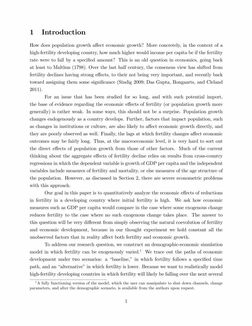
Figure 1: Age-specific fertility rates by time period and demographic scenario

3 Demographic scenarios

As already noted, we divide population into 5-year age groups, and each time period in our

model corresponds to 5 years. Our analysis is focused on considering deviations of the path

of fertility from what would occur along some baseline. Our model can be easily tailored to

consider different baseline and alternative scenarios.

For the analysis in this paper, we tailor the model to fit Nigeria. Specifically, we take

the UN (2010) medium-fertility population projection as our baseline population forecast,

and the UN low-fertility variant as our alternative scenario. The UN reports population by 5-

year age group for every 5-year period through 2100. The UN also reports age-specific fertility

rates for every 5-year period through 2100. Figure 1 shows these age specific fertility rates

for the initial period and then for the final period under the two different fertility scenarios.

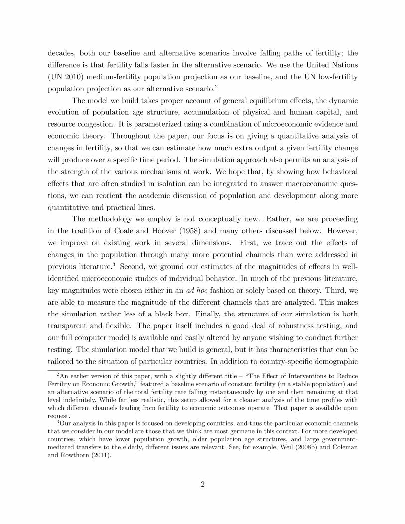
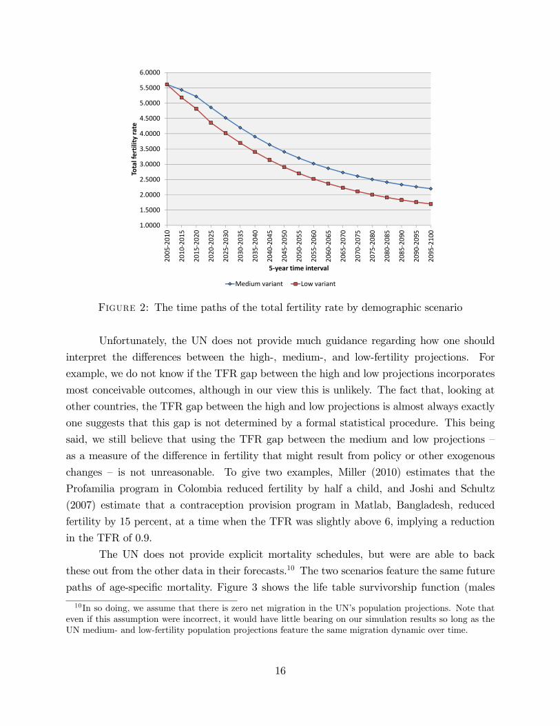
Figure 2 shows the paths of the total fertility rate (TFR) in the two scenarios. The medium

variant has the TFR declining rapidly at first, and then with some slowdown, from 5.61 in

2005—2010 to 4.52 in 2025—2030, and 3.41 in 2045—2050. Fertility in the low variant is the

same as that in the medium variant in 2005—2010, and then differs from the medium variant

by a TFR of 0.25 in 2010—2015, 0.4 in 2015—2020, and by a fixed TFR of 0.5 thereafter. The

difference between the UN high- and medium-fertility variants is the same.

15

1.0000

1.5000

2.0000

2.5000

3.0000

3.5000

4.0000

4.5000

5.0000

5.5000

6.0000

2005

‐2010

2010

‐2015

2015

‐2020

2020

‐2025

2025

‐2030

2030

‐2035

2035

‐2040

2040

‐2045

2045

‐2050

2050

‐2055

2055

‐2060

2060

‐2065

2065

‐2070

2070

‐2075

2075

‐2080

2080

‐2085

2085

‐2090

2090

‐2095

2095

‐2100

Total fertility

 rate

5‐year time interval

Medium variant Low variant

Figure 2: The time paths of the total fertility rate by demographic scenario

Unfortunately, the UN does not provide much guidance regarding how one should

interpret the differences between the high-, medium-, and low-fertility projections. For

example, we do not know if the TFR gap between the high and low projections incorporates

most conceivable outcomes, although in our view this is unlikely. The fact that, looking at

other countries, the TFR gap between the high and low projections is almost always exactly

one suggests that this gap is not determined by a formal statistical procedure. This being

said, we still believe that using the TFR gap between the medium and low projections —

as a measure of the difference in fertility that might result from policy or other exogenous

changes — is not unreasonable. To give two examples, Miller (2010) estimates that the

Profamilia program in Colombia reduced fertility by half a child, and Joshi and Schultz

(2007) estimate that a contraception provision program in Matlab, Bangladesh, reduced

fertility by 15 percent, at a time when the TFR was slightly above 6, implying a reduction

in the TFR of 0.9.

The UN does not provide explicit mortality schedules, but were are able to back

these out from the other data in their forecasts.10 The two scenarios feature the same future

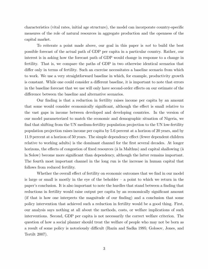
paths of age-specific mortality. Figure 3 shows the life table survivorship function (males

10In so doing, we assume that there is zero net migration in the UN’s population projections. Note thateven if this assumption were incorrect, it would have little bearing on our simulation results so long as theUN medium- and low-fertility population projections feature the same migration dynamic over time.

16

0.0000

0.1000

0.2000

0.3000

0.4000

0.5000

0.6000

0.7000

0.8000

0.9000

1.0000

1.1000

0 5 10 15 20 25 30 35 40 45 50 55 60 65 70 75 80 85 90 95 100

Survivorship ra

te

Beginning year of 5‐year age interval

2005‐2010 (all variants) 2050‐2055 (all variants) 2095‐2100 (all variants)

Figure 3: Age-specific survivorship rates by time period

100

150

200

250

300

350

400

450

500

550

600

650

700

750

2005

2010

2015

2020

2025

2030

2035

2040

2045

2050

2055

2060

2065

2070

2075

2080

2085

2090

2095

2100

Popu

latio

n (in

 millions)

Year

Medium variant Low variant

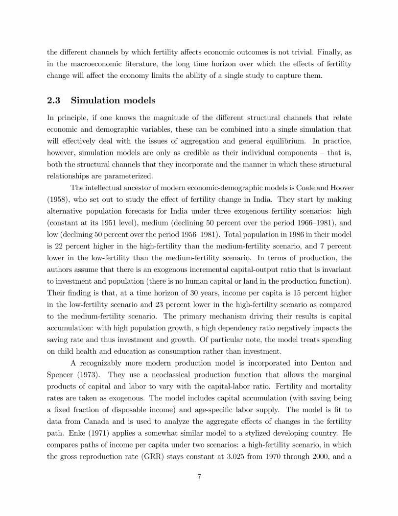
Figure 4: The time paths of population by demographic scenario

17

0.5250

0.5375

0.5500

0.5625

0.5750

0.5875

0.6000

0.6125

0.6250

0.6375

0.6500

0.6625

0.6750

2005

2010

2015

2020

2025

2030

2035

2040

2045

2050

2055

2060

2065

2070

2075

2080

2085

2090

2095

2100

Working

‐age fractio

n of th

e po

pulatio

n

Year

Medium variant Low variant

Figure 5: The time paths of the working-age fraction of the population by demographicscenario

0.1500

0.1750

0.2000

0.2250

0.2500

0.2750

0.3000

0.3250

0.3500

0.3750

0.4000

0.4250

0.4500

2005

2010

2015

2020

2025

2030

2035

2040

2045

2050

2055

2060

2065

2070

2075

2080

2085

2090

2095

2100

Und

er‐15 fractio

n of th

e po

pulatio

n

Year

Medium variant Low variant

Figure 6: The time paths of the under-15 fraction of the population by demographicscenario

18

0.0200

0.0350

0.0500

0.0650

0.0800

0.0950

0.1100

0.1250

0.1400

0.1550

0.1700

2005

2010

2015

2020

2025

2030

2035

2040

2045

2050

2055

2060

2065

2070

2075

2080

2085

2090

2095

2100

Over‐65

 fractio

n of th

e po

pulatio

n

Year

Medium variant Low variant

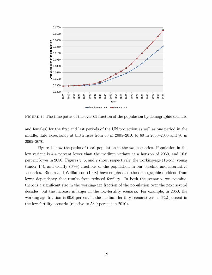
Figure 7: The time paths of the over-65 fraction of the population by demographic scenario

and females) for the first and last periods of the UN projection as well as one period in the

middle. Life expectancy at birth rises from 50 in 2005—2010 to 60 in 2030—2035 and 70 in

2065—2070.

Figure 4 show the paths of total population in the two scenarios. Population in the

low variant is 4.4 percent lower than the medium variant at a horizon of 2030, and 10.6

percent lower in 2050. Figures 5, 6, and 7 show, respectively, the working-age (15-64), young

(under 15), and elderly (65+) fractions of the population in our baseline and alternative

scenarios. Bloom and Williamson (1998) have emphasized the demographic dividend from

lower dependency that results from reduced fertility. In both the scenarios we examine,

there is a significant rise in the working-age fraction of the population over the next several

decades, but the increase is larger in the low-fertility scenario. For example, in 2050, the

working-age fraction is 60.6 percent in the medium-fertility scenario versus 63.2 percent in

the low-fertility scenario (relative to 53.9 percent in 2010).

19

4 Economic model and its parameterization

4.1 Production

In our base case model, aggregate production is given by a standard Cobb-Douglas produc-

tion function. The factor inputs are land (which we use as a shorthand for all fixed factors

of production), physical capital, and effective labor, so that aggregate output in period t, Yt,

is

Yt = AtKαt H

βt X

1−α−β,

where α + β < 1, X is a fixed arbitrary stock of land, and At is productivity.

We assume fairly standard values for factor shares: we set α = 0.3 and β = 0.6,

meaning that the implied share of land is 10 percent. In Section 7, we revisit the role of

fixed factors of production. We consider the sensitivity of our results to both the share of

land in national income and the elasticity of substitution between land and other factors

of production. We also examine data on natural resource shares of national income. For

convenience, we set the growth rate of productivity in the model to zero. The speed of

productivity growth is obviously of paramount importance to the growth of income per

capita, but reasonable variations in this parameter have only trivial effects on the quantity

on which we focus —the ratio of income in the alternative scenario to income in the baseline

scenario.

4.2 Physical capital accumulation

In our base case setup, we handle capital accumulation extremely simply, by following Solow

(1956) in assuming that a fixed share of national income is saved in each period.11 Specifically,

the stock of capital in period t, Kt, evolves over time according to

Kt+1 = sYt + (1− δ)Kt,

where s and δ are the fixed saving and depreciation rates, respectively. We assume that the

annual saving rate is 8.55 percent, which corresponds to the investment share of real GDP

reported by Heston, Summers, and Aten (2009) for Nigeria in 2005. We assign a standard

value of 5 percent to the depreciation rate.

In Section 6, we consider two alternative models of investment. First, we allow for

variable age-specific saving rates, with workers in their prime earning years having higher

11Young (2005) makes the same assumption in his analysis of HIV/AIDS in South Africa.

20

saving rates. This introduces an additional channel though which demographic change affects

growth.12 Second, we consider the case of an economy that is fully open to international

capital flows. This shuts off the Solow channel whereby slower growth of the labor force

raises the level of capital per worker.

4.3 Effective labor

We model an individual’s effective labor as a function of his or her age-specific labor force

participation rate and level of human capital. Human capital, in turn, is a function of his

or her schooling and experience. We assume that human capital inputs of individuals with

different characteristics are perfectly substitutable. Thus, the stock of effective labor in

period t, Ht, is

Ht =∑

15≤i<65

(hsi,t × hei,t × LFPRi,t

)Ni,t,

where Ni,t is the number of individuals of age i in the population in period t, LFPRi,t is

their labor force participation rate, and hsi,t and hei,t are, respectively, their levels of human

capital from schooling and experience. We assume that children enter the labor force at 15

and workers leave the labor force at 65.

In our simulations, we use labor force participation rates reported by the International

Labour Organization (2011) for Nigeria in 2005. Specifically, we employ gender- and age-

specific labor force participation rates to construct total labor force participation rates by

age, using the fraction of males and females in each age group as population weights. Since

our baseline and alternative scenarios both feature forecast paths with declining fertility, we

modify the female labor force participation rates in each future period to reflect the effect of

a decrease in time devoted to child-rearing on total labor supply. This procedure is explained

in Section 4.4.

4.3.1 Returns to schooling

Years of schooling are aggregated into human capital from schooling using a log-linear

specification,

hsi,t = exp[θS],

12There is considerable controversy about the applicability of such models to developing countries. SeeLee, Mason, and Miller (2001) and Deaton (1999).

21

where θ is the return to an additional year of schooling. The return to schooling will be

relevant for the exercises we conduct because reductions in fertility will raise the average

level of schooling.

Estimating the returns to schooling has a long history in economics, going back to at

least Mincer (1974) but beginning as early as the 1950s for the United States. The seminal

works in estimating the Mincerian returns to schooling across different countries in the world

are Psacharopoulos (1973; 1985; 1994) and Psacharopoulos and Patrinos (2004), who find

in the most recent iteration of their results that the returns to schooling in Sub-Saharan

Africa range from 4.1 to 20.1 percent, with an average return of 11.7 percent. These results,

however, have been criticized for being driven by data of poor quality. Banerjee and Duflo

(2005) improve on the quality of these estimates and find a range of 3.3 to 19.1 percent, with

an average return of 9.75 percent.

One concern with these estimates is that they measure the average return to education

in a country. If the change in fertility occurs mostly among low education workers, and the

returns to education differ with the level of education, using the average return to schooling

for all workers may be misleading. Psacharopoulos and Patrinos (2004) do estimate the

returns to education by education level, and they find that the returns fall as the level of

education rises. However, the higher quality estimates from Schultz (2004) indicate the

opposite. He finds that in Nigeria, the return to primary education is approximately 2.5

percent per year, while the return to university education is in the 10-12 percent range.

Moreover, the returns to primary education vary between 2 and 17 percent over a sample of

six African countries, with an average of approximately 8 percent.

Another concern with these estimates is that they are obtained by running OLS

regressions, and therefore the standard econometric concerns of endogeneity and omitted

variables are not addressed. Duflo (2001) exploits a quasi-natural experiment involving a

school building program in Indonesia, and she estimates the returns to education to be

between 6.8 and 10.6 percent. Oyelere (2010) uses a similar research design, exploiting the

provision and then revocation of free primary education in certain regions of Nigeria, to

estimate the returns to education. She finds a return of only 2.8 percent, consistently with

Schultz (2004).

For our base case model, we choose a value of θ = 10 percent, which is the standard

value applied in much of the growth literature and represents a rough average of the estimates

discussed above. In testing for robustness, we examine both Oyelere’s (2010) estimate of 2.8

percent, which has the advantages of being well identified, primary education specific, and

22

based on data for Nigeria, as well as 20 percent, which is the upper bound of estimates from

Banerjee and Duflo (2005) for Sub-Saharan African countries.

4.3.2 Returns to experience

Human capital from on-the-job experience for a worker of age i in period t, hei,t, is computed

as

hei,t = exp[φ(i− 15) + ψ(i− 15)2].

Experience will play a role in our simulations because declines in mortality and fertility will

lead to a population with higher average age and thus higher average experience.

As with the literature on the returns to education, labor economists have been

estimating the returns to experience in the United States since the 1950s. Internationally,

there are a large number of studies with somewhat conflicting results. Estimates of the

Mincerian returns to experience in African nations are highly unreliable due to poor data

quality. The seminal work remains Psacharopoulos (1994), who implicitly estimates the

returns to experience across a set of 45 different countries, in addition to estimating the

returns to education. Unfortunately, Psacharopoulos (1994) does not directly report these

estimates. Bils and Klenow (2000) take the estimates from Psacharopoulos (1994), add seven

additional countries, and report them all in Appendix B of their paper. For our base case

setup, we use values of 0.052 for φ and -0.0009875 for ψ, corresponding to the average of

the estimates for each of these coeffi cients across the four Sub-Saharan African countries

(Botswana, Côte d’Ivoire, Kenya, and Tanzania) in Bils and Klenow (2000).13

4.3.3 Effect of fertility on education

We expect that lower fertility will raise the average level of schooling. Models of the fertility

transition stress the movement of households along a quality-quantity frontier in which

investment per child in health and education rises as the number of children falls. It does not

follow from this observation, however, that the change in schooling that would result from

an exogenous change in fertility is the same as the change that would accompany declining

fertility when both measures are evolving endogenously.

A large literature analyzes the theoretical relationship between the number of siblings

and educational attainment. However, there are few empirical studies from developing

countries that use natural experiments to establish causal estimates of the effect of fertility on

years of schooling. Using data from India, Rosenzweig and Wolpin (1980) and Rosenzweig

13For their full sample of 48 countries, the average values are 0.0495 and -0.0007, respectively.

23

and Schultz (1987) find that an exogenous increase in fertility due to the birth of twins

decreases the level of schooling for all children in a household. Unfortunately, they do not

provide estimates in a form that can be imported into our model. In addition, this work

has faced criticisms due to the imprecision of estimates arising from a small sample size

and methodological problems such as not controlling for birth order. Lee (2008), using the

gender of the first child as an instrument for fertility, finds that higher fertility decreases

educational investment per child in Korean data, but the effect is somewhat small. Using

Norwegian data, Black, Devereux, and Salvanes (2005) find a negative effect of family size

(using twins as a natural experiment) on educational attainment, but the effect disappears

once birth order is controlled for.

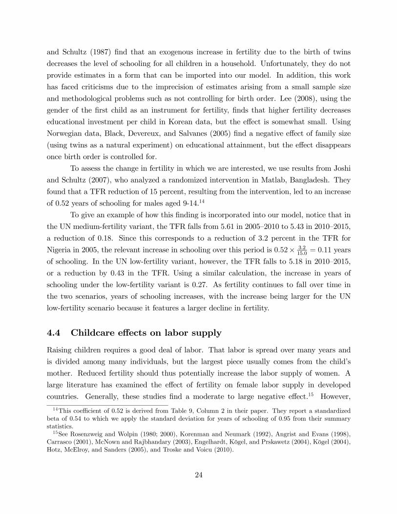
To assess the change in fertility in which we are interested, we use results from Joshi

and Schultz (2007), who analyzed a randomized intervention in Matlab, Bangladesh. They

found that a TFR reduction of 15 percent, resulting from the intervention, led to an increase

of 0.52 years of schooling for males aged 9-14.14

To give an example of how this finding is incorporated into our model, notice that in

the UN medium-fertility variant, the TFR falls from 5.61 in 2005—2010 to 5.43 in 2010—2015,

a reduction of 0.18. Since this corresponds to a reduction of 3.2 percent in the TFR for

Nigeria in 2005, the relevant increase in schooling over this period is 0.52× 3.215.0

= 0.11 years

of schooling. In the UN low-fertility variant, however, the TFR falls to 5.18 in 2010—2015,

or a reduction by 0.43 in the TFR. Using a similar calculation, the increase in years of

schooling under the low-fertility variant is 0.27. As fertility continues to fall over time in

the two scenarios, years of schooling increases, with the increase being larger for the UN

low-fertility scenario because it features a larger decline in fertility.

4.4 Childcare effects on labor supply

Raising children requires a good deal of labor. That labor is spread over many years and

is divided among many individuals, but the largest piece usually comes from the child’s

mother. Reduced fertility should thus potentially increase the labor supply of women. A

large literature has examined the effect of fertility on female labor supply in developed

countries. Generally, these studies find a moderate to large negative effect.15 However,

14This coeffi cient of 0.52 is derived from Table 9, Column 2 in their paper. They report a standardizedbeta of 0.54 to which we apply the standard deviation for years of schooling of 0.95 from their summarystatistics.15See Rosenzweig and Wolpin (1980; 2000), Korenman and Neumark (1992), Angrist and Evans (1998),

Carrasco (2001), McNown and Rajbhandary (2003), Engelhardt, Kögel, and Prskawetz (2004), Kögel (2004),Hotz, McElroy, and Sanders (2005), and Troske and Voicu (2010).

24

surprisingly little research has been done to assess the effect of fertility on female labor

supply outside of Europe and the United States. Among studies focusing on non-Western

countries, Chun and Oh (2002) use sex of the first child as an instrument for fertility in

Korean data, and they find that having an additional child reduces labor force participation

by 40 percent. Bloom et al. (2009) use exogenous changes in abortion laws at the country

level as an instrument for fertility, finding that an additional birth reduces lifetime labor

supply by about two years. However, neither of these papers estimate the effect of fertility

on female labor force participation strictly in a developing country, where one would expect

the effect of fertility on female labor force participation to be lower since child-rearing is often

combined with productive activities. A handful of studies focusing on developing countries

are currently underway, but this literature is still in its infancy.16

Beyond the general lack of research in this area, assigning a quantitative magnitude

to the effect of fertility on female labor supply is diffi cult for several reasons.

• There are obviously strong economies of scale in child-rearing —the time cost associatedwith the first child is far higher than the marginal time cost of subsequent children.

For example, Tiefenthaler (1997), examining data from Cebu, Philippines, finds that

14 months after birth, female labor market hours had declined by 39 percent in the

case of first births, but by only 10 percent if there were already children aged 0-5 in the

household. If there were both children aged 0-5 and children aged 6-17 in the household,

female labor market hours were actually slightly higher at 14 months following a birth.

• Not all time spent on children is subtracted from production. A good part of time

devoted to child-rearing may be at the expense of leisure or, in the case of siblings,

human capital investment (which is not counted as part of national income).

• Child-rearing is often combined with productive activities, especially in developingcountries. For example, a woman may carry a baby in a sling or watch children out

of the corner of her eye while she works at a productive task. In this case, the cost of

child-rearing in terms of productive labor would only be the decrement in productivity

that results from such multitasking.

Despite these caveats, the time cost of child-rearing may still be a significant compo-

nent in the economic response to fertility decline. We measure the effect of fertility change

on labor supply through the childcare channel by specifying a parameter we call the labor

16Porter and King (2012) use the advent of twins as an unanticipated shock to fertility to estimate theeffect of fertility on female labor force participation, and find there is little effect.

25

market time cost of a marginal child. Summarizing all these considerations in a single

parameter is obviously too simplistic but, in doing so, we at least have a concrete measure

that can be implemented in our model. Specifying the time cost of the marginal child might

also be considered problematic because the marginal cost would be expected to fall with

the number of children. However, Holmes and Tiefenthaler (1997) conclude the that the

marginal time cost of children is roughly constant for the third and higher children, and for

the experiments we are considering, the TFR generally remains above two.17

Mechanically, we implement the childcare effect by increasing female labor force

participation in each year by the hypothesized change in age-specific fertility multiplied by

the labor market time cost (in years) of a marginal child. For example, if in our experiment,

age-specific fertility of women aged 25-29 drops from 0.2646 to 0.2179 (as it does in the UN

medium-fertility scenario between 2005—2010 and 2045—2050), and if the labor market time

cost of a marginal child is one year, then labor force participation for women in this age

group would rise by 4.67 percentage points.18

There only remains the question of choosing the base case parameter value for the

time cost of children. In the Cebu data used by Tiefenthaler (1997), weekly labor market

hours fall from 10.4 prenatally to 5.0 at two months, 6.6 at six months, and 9.5 at 14 months

for women who have other children aged 0-5 in the household; and from 13.1 prenatally to 7.6

at two months, 11.3 at six months, and 13.8 at 14 months for those with children aged both

0-5 and 6-17 in the household. Crudely interpolating these data, and allowing for an almost

total cessation of labor market activity in the first month after delivery, hours averaged over

the first year are reduced roughly 5 per week in the first group and 3 per week for the second

group. Weekly labor market hours for men in the same households do not change much

in response to a birth, and are equal to roughly 40. So, in this data, women in these two

groups lose 0.125 or 0.075 years of full-time equivalent labor market input in the first year

after the birth of a marginal child. The complete or nearly complete recovery of labor hours

17Because of heterogeneity in completed fertility, a reduction in the TFR from three to two will not meanthat all children not born would have been parity three. Instead, some would have been higher parity, whileothers would have been first or second children. Thus, our method will understate the increase in labor inputthat results from such a reduction in fertility.18Although it might seem problematic to “charge” the entire time cost of a child to the mother in the

year of the child’s birth, we do not view this as too distortionary of reality for two reasons. First, timecosts of child-rearing are indeed concentrated in the first years of life. Second, because we are considering anage-specific fertility schedule that assigns a fractional number of births per year to each woman, the patternof labor force increase that is generated by our method will look similar to what would result if each birthreduced labor force participation over a longer period of time. It is true, however, that our method mayslightly front-load the effect of lower fertility on labor force participation, both because we ignore child-rearing costs in later years and also because we apply our marginal rate to all births, whereas higher orderbirths are concentrated at older ages.

26

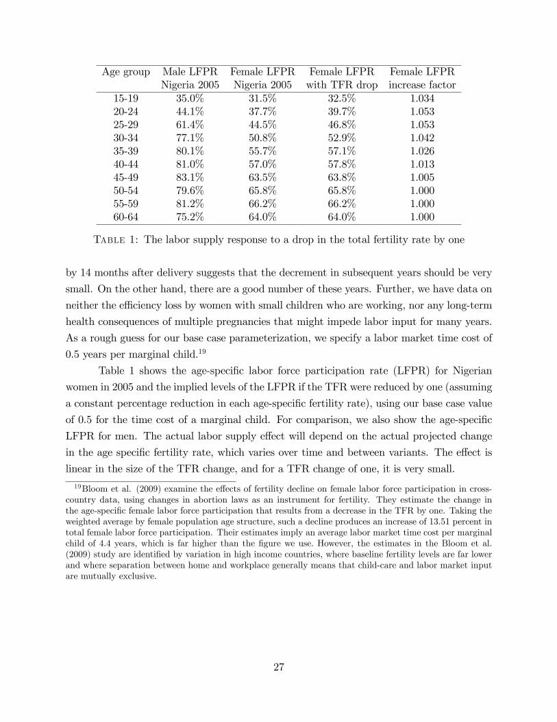
Age group Male LFPR Female LFPR Female LFPR Female LFPRNigeria 2005 Nigeria 2005 with TFR drop increase factor

15-19 35.0% 31.5% 32.5% 1.03420-24 44.1% 37.7% 39.7% 1.05325-29 61.4% 44.5% 46.8% 1.05330-34 77.1% 50.8% 52.9% 1.04235-39 80.1% 55.7% 57.1% 1.02640-44 81.0% 57.0% 57.8% 1.01345-49 83.1% 63.5% 63.8% 1.00550-54 79.6% 65.8% 65.8% 1.00055-59 81.2% 66.2% 66.2% 1.00060-64 75.2% 64.0% 64.0% 1.000

Table 1: The labor supply response to a drop in the total fertility rate by one

by 14 months after delivery suggests that the decrement in subsequent years should be very

small. On the other hand, there are a good number of these years. Further, we have data on

neither the effi ciency loss by women with small children who are working, nor any long-term

health consequences of multiple pregnancies that might impede labor input for many years.

As a rough guess for our base case parameterization, we specify a labor market time cost of

0.5 years per marginal child.19

Table 1 shows the age-specific labor force participation rate (LFPR) for Nigerian

women in 2005 and the implied levels of the LFPR if the TFR were reduced by one (assuming

a constant percentage reduction in each age-specific fertility rate), using our base case value

of 0.5 for the time cost of a marginal child. For comparison, we also show the age-specific

LFPR for men. The actual labor supply effect will depend on the actual projected change

in the age specific fertility rate, which varies over time and between variants. The effect is

linear in the size of the TFR change, and for a TFR change of one, it is very small.

19Bloom et al. (2009) examine the effects of fertility decline on female labor force participation in cross-country data, using changes in abortion laws as an instrument for fertility. They estimate the change inthe age-specific female labor force participation that results from a decrease in the TFR by one. Taking theweighted average by female population age structure, such a decline produces an increase of 13.51 percent intotal female labor force participation. Their estimates imply an average labor market time cost per marginalchild of 4.4 years, which is far higher than the figure we use. However, the estimates in the Bloom et al.(2009) study are identified by variation in high income countries, where baseline fertility levels are far lowerand where separation between home and workplace generally means that child-care and labor market inputare mutually exclusive.

27

4.5 Other channels not covered

A simulation study such as ours is useful only to the extent that it covers all of the quantita-

tively important channels through which a change in fertility affects the macroeconomy. We

have tried to keep our framework transparent and open, so that we (or someone else) can

add other channels if there is an appropriate basis. Here, we discuss some potential channels

that we have not included, either because we think that they are of secondary quantitative

importance or because we did not have a basis for quantifying them.

4.5.1 Boserup effects

There are several channels through which higher population density could positively affect

the level of income per capita. In the context of agriculture, Boserup (1965) stressed that,

as population rose, farmers were induced to switch to more intensive methods, which meant

that the land constraint did not end up lowering income per worker. A more generalized

version of this effect would be that higher population would induce technological progress

more generally, that is outside of agriculture, either out of “necessity,” or because more

people raises the likelihood of someone having a productive idea (Jones 1995). A completely

different channel by which population growth could raise output would be by allowing for

better trade and economies of scale in production. In the African context, it is often noted

that long distances and poor roads lead to an extremely high cost of trade.

We do not include any of these channels in our analysis for several reasons. Regarding

agriculture, some of the possibilities for intensification and substitution of other inputs for

land are already included in our production function approach. In particular, Section 7 (and

the literature on which it draws) discusses evidence on the substitutability of other inputs

for land. The intensity of cultivation varies enormously in Sub-Saharan Africa, but the

Boserupian description in which fertile land can easily be shifted from fallow to continuous

cultivation seems inappropriate for most countries. Indeed, data show that over the last

decades cultivation in Africa has increasingly expanded onto marginally suitable land (Weil

2008a).

Regarding gains from scale as population rises, we are of two minds. On the one

hand, we agree that costly transport raises trade costs and leads to an ineffi cient scale of

production in many African countries (Gollin and Rogerson 2009). However, it is not clear

that population growth over the next several decades will lead to increases in rural population

density that would facilitate trade. Rather, Africa is rapidly urbanizing, implying that much

of the growth of population in the next decades will end up in already large cities (Weil

28

2008a). It is hard to believe that mega cities such as Lagos do not already have suffi cient

size to achieve economies of scale in production.

On a more prosaic level, we were not able to find quantitative estimates of the size of

Boserup effects that we could incorporate into our model.

4.5.2 Effects through health improvements

Another channel through which fertility declines could possibly affect output is through

improvements in health. These could result from the same quality-quantity shift that we

model in the case of education. Ashraf, Lester, and Weil (2008) discuss how improvements

in health can be translated quantitatively into productive human capital. However, Joshi

and Schultz (2007) find no effect of the fertility intervention in Matlab, Bangladesh on child

health.

5 Basic results

Figure 8 shows the paths of physical capital per worker, human capital per worker, labor

input per worker, income per worker, and income per capita in our simulation, using the

base case parameters discussed above. The path of output per worker reflects the dynamics

of human and physical capital per worker, labor input per worker, and land per worker

(which we do not show, but which can be inferred from Figure 8). As in all the figures that

follow, we show the ratio of outcomes in the alternative scenario to outcomes in the baseline

scenario. Further, in discussing our simulation results below, we refer to the year 2010 (that

is, the last year before fertility in the baseline and alternative scenarios begin to diverge)

as the start of our simulation, so references to time horizons in our simulation should be

interpreted with respect to this year.

Figure 8 shows that, in our base case setup, the long-run effect of reducing fertility

from the UN medium variant to the low variant is to raise output per capita by 11.9 percent

at a horizon of 50 years. At a 20-year horizon, the increase in income per capita is 5.6

percent.20 Because fertility in the alternative scenario is lower than in the baseline scenario

for the entire period we examine, income in the two scenarios continues to diverge.

20Using the UN high-fertility and medium-fertility population projections as our baseline and alternativescenarios, respectively, the increase in income per capita resulting from lower fertility is 11.5 percent at ahorizon of 50 years, and 5.4 percent at a horizon of 20 years. Since the difference in the TFR (at any pointin time) between the high- and medium-fertility scenarios is the same as that between the medium- andlow-fertility scenarios, and because all three scenarios feature identical assumptions about mortality (andnet migration) rates, the effect of fertility reduction under our base case setup is roughly linear in the sizeof the reduction.

29

0.9750

1.0000

1.0250

1.0500

1.0750

1.1000

1.1250

1.1500

1.1750

1.2000

1.2250

1.2500

2005

2010

2015

2020

2025

2030

2035

2040

2045

2050

2055

2060

2065

2070

2075

2080

2085

2090

2095

2100

Values (low

‐relative to m

edium‐variant)

Year

Physical capital per worker Human capital per worker Labor supply per worker

Income per worker Income per capita

Figure 8: The base case economic projection

Before going further, it is of interest to compare the findings of our simulation model

with results from other studies. We focus on Bloom and Canning (2008), a well-cited cross-

country regression study that appeared in this Review. In that paper, the independent

variable of interest is the growth rate of the working-age fraction of the population, and

the dependent variable is the growth rate of income per capita. The relevant coeffi cient is

estimated at 0.996 using a simple OLS regression, and at 1.394 when the authors use lagged

endogenous variables as instruments.

To compare the Bloom and Canning (2008) findings to our results, we first look at

the growth rate of the working-age fraction of the population in our baseline and alternative

scenarios. In both scenarios, the working-age fraction is 0.5379 in 2010, the first year of

our simulation. Under the medium-fertility scenario, the fraction rises to 0.6252 in the year

2060, but it rises to 0.6532 under the low-fertility scenario. The implied annual growth rates

of the working-age fraction are 0.301 percent per year in the medium-fertility variant and

0.389 percent per year in the low-fertility variant. To get the effect of lower fertility on

income growth, we multiply the difference between these two growth rates (that is, 0.088

percent per year) by the Bloom and Canning (2008) coeffi cient. This yields an income growth

differential (between the two scenarios) of 0.088 percent per year using their OLS estimate

and 0.123 percent per year using their IV estimate. By contrast, in our simulation, the

change in fertility from the medium to the low variant leads to income per capita rising by

30

11.9 percent over the first 50 years of the simulation, implying an increment to growth of

0.225 percent per year. In other words, the effect that we find in our simulation is roughly

twice as large as theirs.

5.1 Component channels

As discussed above, demographic change affects economic outcomes through a number of

channels, which may operate at different relative intensities at different time horizons. It

is of interest to decompose the overall effect of fertility reduction into the parts that run

through these different channels. Some caution is necessary, however, because there are

clearly interactions among the different effects. In particular, the effect of fertility through

any one channel will depend on which other channels are operative. For example, the effect of

increased labor force participation of working-age adults will be larger or smaller, depending

on the fraction of the population made up of such adults. To address this problem, we do

all of our analysis of the effects of fertility through each of the different channels under the

assumption that all the other channels are operative —that is, we consider the results in our

full simulation relative to the case where one channel is “deleted”(an alternative would be

to assume that no other channels were operative).

We begin by looking at several channels individually. This allows us to perform an

analysis of the sensitivity of our results to assumptions about key parameters. We then do

a full decomposition, showing the relative importance of the different channels at different

time horizons.

To gauge the importance of non-reproducible factors, we conduct a simulation in

which the level of land per worker in the alternative scenario follows the same path as

it does in the baseline scenario. In other words, we ignore the effect of lower fertility in

preventing the land-labor ratio from falling, while allowing for all the other economic effects

of fertility decline. Figure 9 compares the path of output per capita in this case to the

base case. The figure illustrates the extent to which the classic Malthusian channel operates

only over relatively long time horizons. For the first 35 years of the simulation, the path of

income per capita when the Malthus effect is suppressed looks only slightly different than

when the effect is present (for the first 15 of these years, this is mechanically true because

the ratio of land to labor is the same across the baseline and alternative scenarios). In the

longer run, however, the effect of reduced congestion of the fixed factor becomes prominent

—at an 80-year horizon, income per capita is only 11.1 percent above baseline with the effect

suppressed, versus 15.1 percent above baseline with the effect present.

31

0.9800

1.0000

1.0200

1.0400

1.0600

1.0800

1.1000

1.1200

1.1400

1.1600

1.1800

2005

2010

2015

2020

2025

2030

2035

2040

2045

2050

2055

2060

2065

2070

2075

2080

2085

2090

2095

2100

Income pe

r cap

ita (low

‐relative to m

edium‐variant)

Year

Variable land‐labor ratio (base case) Fixed land‐labor ratio

Figure 9: The effect of the land-labor ratio on income per capita

We conduct a similar exercise to look at the importance of the capital-shallowing

channel. Specifically, we examine the case in which the level of physical capital per worker

is the same in the alternative scenario as it is in the baseline scenario. The result is shown

in Figure 10. As with the Malthus effect, for the first 15 years of the simulation, suppressing

the Solow effect makes no difference to the level of income per capita because the number of

workers does not differ between the baseline and alternative scenarios. At year 50, output

per capita is 8.8 percent above baseline when the Solow effect is suppressed, compared to

11.9 percent above baseline when the Solow effect is present.

Figure 11 shows the dependency effect, comparing the base case to the case where the

dependency ratio in the alternative scenario is fixed to remain the same as in the baseline

scenario. Here, not surprisingly, the phase-in of the effect is almost immediate. Fifteen years

after the beginning of the simulation, income per capita is only 1.8 percent above baseline

when the dependency effect is suppressed, versus 4.2 percent above baseline when the effect

is present. By year 50, the increase in income per capita is 5.2 percentage points higher in

the base case than in the case where the dependency effect is suppressed. From this point

onward, the difference between the two paths appears roughly constant.

Figure 12 looks at the experience channel. We compare the base case to the case

where the experience effect is shut down (by assuming that the return to experience is zero).

As the figure shows, the experience effect is not of great import. For example, at a 50 year

32

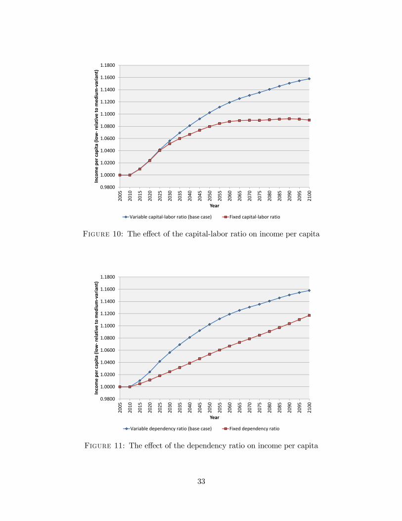
0.9800

1.0000

1.0200

1.0400

1.0600

1.0800

1.1000

1.1200

1.1400

1.1600

1.1800

2005

2010

2015

2020

2025

2030

2035

2040

2045

2050

2055

2060

2065

2070

2075

2080

2085

2090

2095

2100

Income pe

r cap

ita (low

‐relative to m

edium‐variant)

Year

Variable capital‐labor ratio (base case) Fixed capital‐labor ratio

Figure 10: The effect of the capital-labor ratio on income per capita

0.9800

1.0000

1.0200

1.0400

1.0600

1.0800

1.1000

1.1200

1.1400

1.1600

1.1800

2005

2010

2015

2020

2025

2030

2035

2040

2045

2050

2055

2060

2065

2070

2075

2080

2085

2090

2095

2100

Income pe

r cap

ita (low

‐relative to m

edium‐variant)

Year

Variable dependency ratio (base case) Fixed dependency ratio

Figure 11: The effect of the dependency ratio on income per capita

33

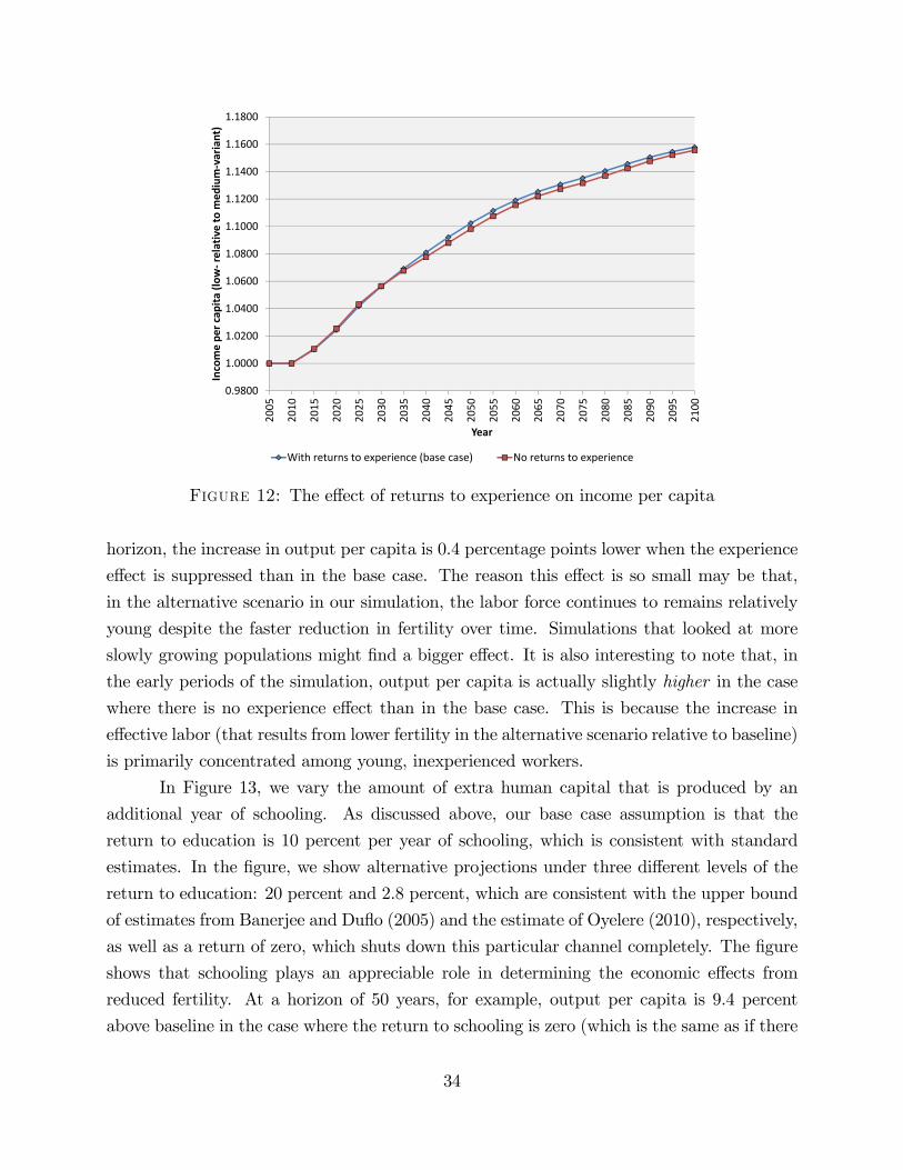
0.9800

1.0000

1.0200

1.0400

1.0600

1.0800

1.1000

1.1200

1.1400

1.1600

1.1800

2005

2010

2015

2020

2025

2030

2035

2040

2045

2050

2055

2060

2065

2070

2075

2080

2085

2090

2095

2100

Income pe

r cap

ita (low

‐relative to m

edium‐variant)

Year

With returns to experience (base case) No returns to experience

Figure 12: The effect of returns to experience on income per capita

horizon, the increase in output per capita is 0.4 percentage points lower when the experience

effect is suppressed than in the base case. The reason this effect is so small may be that,

in the alternative scenario in our simulation, the labor force continues to remains relatively

young despite the faster reduction in fertility over time. Simulations that looked at more

slowly growing populations might find a bigger effect. It is also interesting to note that, in

the early periods of the simulation, output per capita is actually slightly higher in the case

where there is no experience effect than in the base case. This is because the increase in

effective labor (that results from lower fertility in the alternative scenario relative to baseline)

is primarily concentrated among young, inexperienced workers.

In Figure 13, we vary the amount of extra human capital that is produced by an

additional year of schooling. As discussed above, our base case assumption is that the

return to education is 10 percent per year of schooling, which is consistent with standard

estimates. In the figure, we show alternative projections under three different levels of the

return to education: 20 percent and 2.8 percent, which are consistent with the upper bound

of estimates from Banerjee and Duflo (2005) and the estimate of Oyelere (2010), respectively,

as well as a return of zero, which shuts down this particular channel completely. The figure

shows that schooling plays an appreciable role in determining the economic effects from

reduced fertility. At a horizon of 50 years, for example, output per capita is 9.4 percent

above baseline in the case where the return to schooling is zero (which is the same as if there

34

0.9800

1.0000

1.0200

1.0400

1.0600

1.0800

1.1000

1.1200

1.1400

1.1600

1.1800

1.2000

2005

2010

2015

2020

2025

2030

2035

2040

2045

2050

2055

2060

2065

2070

2075

2080

2085

2090

2095

2100

Income pe

r cap

ita (low

‐relative to m

edium‐variant)

Year

Medium returns to schooling (base case) High returns Low returns No returns

Figure 13: The effect of returns to schooling on income per capita

were no increase in schooling), versus 11.9 percent higher in the base case. Thus, roughly

speaking, schooling accounts for one quarter of the income gain (from lower fertility in the

alternative scenario relative to baseline) at this time horizon.

As would be expected, the effect of higher schooling due to lower fertility phases in

as the cohorts that received the additional schooling enter the labor force and replace those

that did not. Thus, for the first 15 years of the simulation this channel contributes little to

higher income.

Figure 14 examines the childcare channel. We consider variations in the parameter

reflecting the time cost of a marginal child. Specifically, we compare the path of income

per capita using our base case assumption of a cost per marginal child of 0.5 years (of labor

market input) to alternatives of one and zero. The channel turns out to be rather weak. At

a horizon of 15 years, for example, income per capita is 4.2 percent above baseline when the

marginal cost of a child is at its base case value of 0.5, versus 4.5 percent above baseline

when the marginal cost of a child is one, and 3.8 percent above baseline when the marginal

cost of a child is zero.

Finally, Figure 15 shows the life-cycle labor supply effect. We compare the base

case parameterization of our model to the case where labor force participation rates are

constant across age groups. Like the experience channel, the life-cycle labor supply channel

has a relatively modest effect on income per capita. After a horizon of 50 years, income per

35

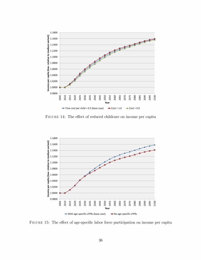
0.9800

1.0000

1.0200

1.0400

1.0600

1.0800

1.1000

1.1200

1.1400

1.1600

1.1800

2005

2010

2015

2020

2025

2030

2035

2040

2045

2050

2055

2060

2065

2070

2075

2080

2085

2090

2095

2100

Income pe

r cap

ita (low

‐relative to m

edium‐variant)

Year

Time cost per child = 0.5 (base case) Cost = 1.0 Cost = 0.0

Figure 14: The effect of reduced childcare on income per capita

0.9800

1.0000

1.0200

1.0400

1.0600

1.0800

1.1000

1.1200

1.1400

1.1600

1.1800

2005

2010

2015

2020

2025

2030

2035

2040

2045

2050

2055

2060

2065

2070

2075

2080

2085

2090

2095

2100

Income pe

r cap

ita (low

‐relative to m

edium‐variant)

Year

With age‐specific LFPRs (base case) No age‐specific LFPRs

Figure 15: The effect of age-specific labor force participation on income per capita

36

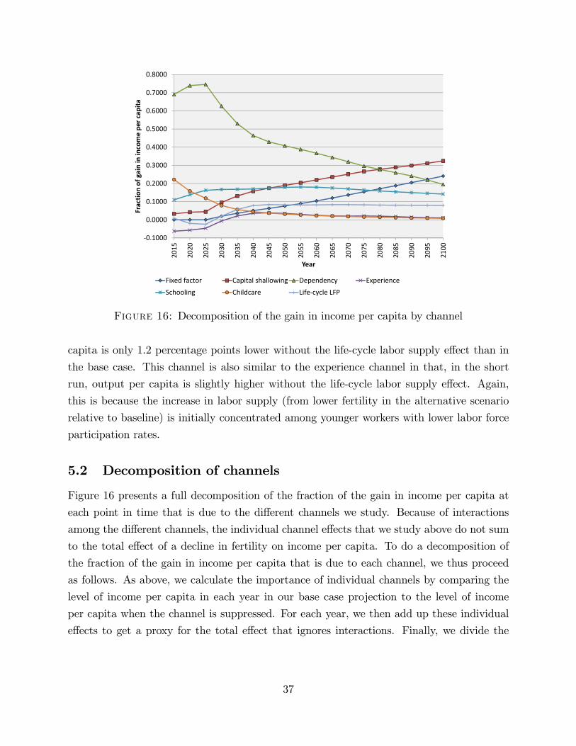
‐0.1000

0.0000

0.1000

0.2000

0.3000

0.4000

0.5000

0.6000

0.7000

0.8000

2015

2020

2025

2030

2035

2040

2045

2050

2055

2060

2065

2070

2075

2080

2085

2090

2095

2100

Fractio

n of gain in income pe

r cap

ita

Year

Fixed factor Capital shallowing Dependency Experience

Schooling Childcare Life‐cycle LFP

Figure 16: Decomposition of the gain in income per capita by channel

capita is only 1.2 percentage points lower without the life-cycle labor supply effect than in

the base case. This channel is also similar to the experience channel in that, in the short

run, output per capita is slightly higher without the life-cycle labor supply effect. Again,

this is because the increase in labor supply (from lower fertility in the alternative scenario

relative to baseline) is initially concentrated among younger workers with lower labor force

participation rates.

5.2 Decomposition of channels

Figure 16 presents a full decomposition of the fraction of the gain in income per capita at

each point in time that is due to the different channels we study. Because of interactions

among the different channels, the individual channel effects that we study above do not sum

to the total effect of a decline in fertility on income per capita. To do a decomposition of

the fraction of the gain in income per capita that is due to each channel, we thus proceed

as follows. As above, we calculate the importance of individual channels by comparing the

level of income per capita in each year in our base case projection to the level of income

per capita when the channel is suppressed. For each year, we then add up these individual

effects to get a proxy for the total effect that ignores interactions. Finally, we divide the

37

individual effects by the proxy (for the total) to produce a share of the total income gain

due to each effect at each time horizon.

The figure shows that the dependency effect is by far the dominant channel in the

short run, explaining roughly 70 percent of the income gain in the first 15 years of the

simulation, and only falling below 40 percent of the total after 45 years. The childcare effect,

which is conceptually very similar to the dependency effect, has a somewhat comparable

trajectory, although at a much lower level. At a horizon of 50 years, the four dominant

effects are dependency (36.7 percent of the total gain), Solow (22.0 percent), schooling (18.0

percent), and Malthus (10.4 percent). At a horizon of 90 years, the same four effects are

dominant, but in a different order: Solow (32.4 percent), Malthus (24.1 percent), dependency

(19.5 percent), and schooling (14.2 percent).

6 Alternative models of investment

6.1 Age-specific saving rates

Discussions of the demographic dividend from reduced population growth, such as Bloom

and Williamson (1998), have often stressed the benefits to national saving from having a

large fraction of the population in its working years. In addition to raising income directly

by lowering the dependency ratio, the capital accumulation from this extra saving can result

in an increase in output per worker. In this section, we explore incorporating such effects

into our model.

One way to incorporate a demographic effect on national savings would be to combine

data on age-specific saving rates with the evolving age structure of the population in each

demographic scenario we examine. Poterba (1994) presents data on age-specific saving rates

in a number of developed countries. However, such data are generally not available for

developing countries, and the data that do exist show little to no evidence of life-cycle

saving behavior. For example, Deaton (1992) calculates household consumption and income

over the life cycle in Côte d’Ivoire, finding no clear relationship between age and saving,

consumption, or even income. Beyond this lack of data, there is a theoretical problem in

looking at age-specific saving rates. Weil (1994) points out that data on age-specific saving

does not take into account the externality effects across generations via support of children

and the aged, bequests, and other transfers. As the age structure of the population changes,

so do these intergenerational flows. To give a simple example, consider a reduction in the

number of children aged 0-4 in a population, holding fixed the numbers of people in all other

38

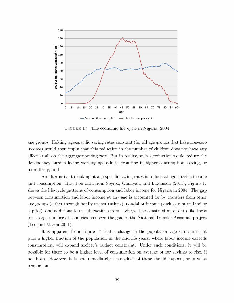
0

20

40

60

80

100

120

140

160

180

0 5 10 15 20 25 30 35 40 45 50 55 60 65 70 75 80 85 90+

2004

 value

s (in th

ousand

s of N

iara)

Age

Consumption per capita Labor income per capita

Figure 17: The economic life cycle in Nigeria, 2004

age groups. Holding age-specific saving rates constant (for all age groups that have non-zero

income) would then imply that this reduction in the number of children does not have any

effect at all on the aggregate saving rate. But in reality, such a reduction would reduce the

dependency burden facing working-age adults, resulting in higher consumption, saving, or

more likely, both.

An alternative to looking at age-specific saving rates is to look at age-specific income

and consumption. Based on data from Soyibo, Olaniyan, and Lawanson (2011), Figure 17

shows the life-cycle patterns of consumption and labor income for Nigeria in 2004. The gap

between consumption and labor income at any age is accounted for by transfers from other

age groups (either through family or institutions), non-labor income (such as rent on land or

capital), and additions to or subtractions from savings. The construction of data like these

for a large number of countries has been the goal of the National Transfer Accounts project

(Lee and Mason 2011).

It is apparent from Figure 17 that a change in the population age structure that

puts a higher fraction of the population in the mid-life years, where labor income exceeds

consumption, will expand society’s budget constraint. Under such conditions, it will be

possible for there to be a higher level of consumption on average or for savings to rise, if

not both. However, it is not immediately clear which of these should happen, or in what

proportion.

39

The piece of data missing from Figure 17 is non-labor income. To calculate this,

we start with data on the aggregate national saving rate in Nigeria in 2005, from Heston,

Summers, and Aten (2009), which was 8.55 percent. We impute total non-labor income such

that, given the consumption and labor income profiles, as well as the age structure of the

population, we exactly match this saving rate. That is, defining x2005 as non-labor income

per capita in 2005, and ci and wi as consumption per capita and labor income per capita,

respectively, at age i,

0.0855 = 1−[100∑i=0

Ni,2005ci

]/

[x2005

100∑i=0

Ni,2005 +

100∑i=0

Ni,2005wi

].

In the Nigerian data that we use as a benchmark, the level of x2005 is 30,586 Niara per capita.

This implies that non-labor income is 44 percent of total income, which is not inconsistent

with our model in which production is Cobb-Douglas and labor’s share of national income

is 60 percent, capital’s share is 30 percent, and land’s share is 10 percent.

We can now look more explicitly at how changes in demographic structure affect

consumption possibilities. When the age structure of the population changes, labor income

per capita shifts, because people at different ages have different levels of labor income. In

addition, however, the consumption “needs” of the population also change. Although we

do not model this explicitly, we assume that the varying pattern of consumption by age

reflects both changing biological needs for consumption over the course of the life cycle and

the arrangements by which consumption is divided up among different groups in society.

For simplicity, we assume that these relative levels of consumption do not change as the

age structure of the population changes, and we call them consumption needs, even though

this is not very good terminology. Slower population growth, by reducing the fraction of

the population made up of children, puts more people in ages that have higher relative

consumption —this effect undoes some of the benefit of having more people earning labor

income.

Putting together the change in labor income and the change in consumption needs,

we can calculate the demographically-induced increase in available demographically-adjusted

income less demographically-adjusted consumption needs relative to a base year of 2005.21

We call this term the change in disposable income (∆DIt), which is again a slight abuse of

21This approach is derived from Lee (1980).

40

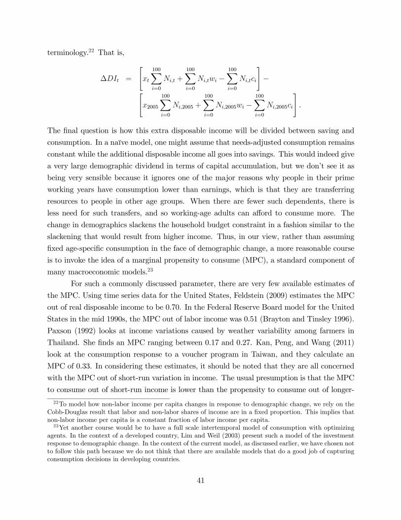
terminology.22 That is,

∆DIt =

[xt

100∑i=0

Ni,t +

100∑i=0

Ni,twi −100∑i=0

Ni,tci

]−[

x2005

100∑i=0

Ni,2005 +

100∑i=0

Ni,2005wi −100∑i=0

Ni,2005ci

].

The final question is how this extra disposable income will be divided between saving and

consumption. In a naïve model, one might assume that needs-adjusted consumption remains

constant while the additional disposable income all goes into savings. This would indeed give

a very large demographic dividend in terms of capital accumulation, but we don’t see it as

being very sensible because it ignores one of the major reasons why people in their prime

working years have consumption lower than earnings, which is that they are transferring

resources to people in other age groups. When there are fewer such dependents, there is

less need for such transfers, and so working-age adults can afford to consume more. The

change in demographics slackens the household budget constraint in a fashion similar to the

slackening that would result from higher income. Thus, in our view, rather than assuming

fixed age-specific consumption in the face of demographic change, a more reasonable course

is to invoke the idea of a marginal propensity to consume (MPC), a standard component of

many macroeconomic models.23

For such a commonly discussed parameter, there are very few available estimates of

the MPC. Using time series data for the United States, Feldstein (2009) estimates the MPC

out of real disposable income to be 0.70. In the Federal Reserve Board model for the United

States in the mid 1990s, the MPC out of labor income was 0.51 (Brayton and Tinsley 1996).

Paxson (1992) looks at income variations caused by weather variability among farmers in

Thailand. She finds an MPC ranging between 0.17 and 0.27. Kan, Peng, and Wang (2011)

look at the consumption response to a voucher program in Taiwan, and they calculate an

MPC of 0.33. In considering these estimates, it should be noted that they are all concerned

with the MPC out of short-run variation in income. The usual presumption is that the MPC

to consume out of short-run income is lower than the propensity to consume out of longer-

22To model how non-labor income per capita changes in response to demographic change, we rely on theCobb-Douglas result that labor and non-labor shares of income are in a fixed proportion. This implies thatnon-labor income per capita is a constant fraction of labor income per capita.23Yet another course would be to have a full scale intertemporal model of consumption with optimizing

agents. In the context of a developed country, Lim and Weil (2003) present such a model of the investmentresponse to demographic change. In the context of the current model, as discussed earlier, we have chosen notto follow this path because we do not think that there are available models that do a good job of capturingconsumption decisions in developing countries.

41

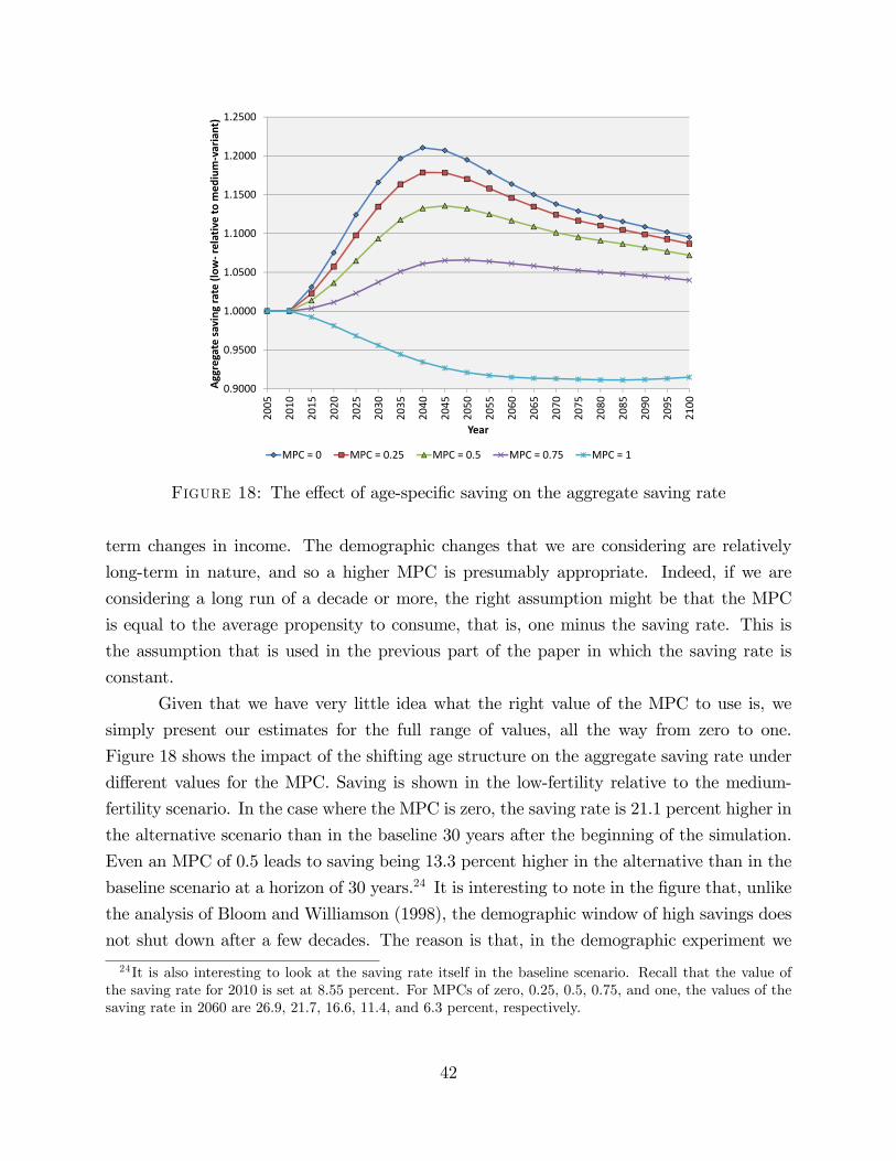
0.9000

0.9500

1.0000

1.0500

1.1000

1.1500

1.2000

1.2500

2005

2010

2015

2020

2025

2030

2035

2040

2045

2050

2055

2060

2065

2070

2075

2080

2085

2090

2095

2100

Aggregate saving

 rate (low

‐relative to m

edium‐variant)

Year

MPC = 0 MPC = 0.25 MPC = 0.5 MPC = 0.75 MPC = 1

Figure 18: The effect of age-specific saving on the aggregate saving rate

term changes in income. The demographic changes that we are considering are relatively

long-term in nature, and so a higher MPC is presumably appropriate. Indeed, if we are

considering a long run of a decade or more, the right assumption might be that the MPC

is equal to the average propensity to consume, that is, one minus the saving rate. This is

the assumption that is used in the previous part of the paper in which the saving rate is

constant.

Given that we have very little idea what the right value of the MPC to use is, we

simply present our estimates for the full range of values, all the way from zero to one.

Figure 18 shows the impact of the shifting age structure on the aggregate saving rate under

different values for the MPC. Saving is shown in the low-fertility relative to the medium-

fertility scenario. In the case where the MPC is zero, the saving rate is 21.1 percent higher in

the alternative scenario than in the baseline 30 years after the beginning of the simulation.

Even an MPC of 0.5 leads to saving being 13.3 percent higher in the alternative than in the

baseline scenario at a horizon of 30 years.24 It is interesting to note in the figure that, unlike

the analysis of Bloom and Williamson (1998), the demographic window of high savings does

not shut down after a few decades. The reason is that, in the demographic experiment we

24It is also interesting to look at the saving rate itself in the baseline scenario. Recall that the value ofthe saving rate for 2010 is set at 8.55 percent. For MPCs of zero, 0.25, 0.5, 0.75, and one, the values of thesaving rate in 2060 are 26.9, 21.7, 16.6, 11.4, and 6.3 percent, respectively.

42

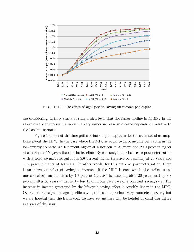
0.9750

1.0000

1.0250

1.0500

1.0750

1.1000

1.1250

1.1500

1.1750

1.2000

1.2250

2005

2010

2015

2020

2025

2030

2035

2040

2045

2050

2055

2060

2065

2070

2075

2080

2085

2090

2095

2100

Income pe

r cap

ita (low

‐relative to m

edium‐variant)

Year

No ASSR (base case) ASSR, MPC = 0 ASSR, MPC = 0.25

ASSR, MPC = 0.5 ASSR, MPC = 0.75 ASSR, MPC = 1

Figure 19: The effect of age-specific saving on income per capita

are considering, fertility starts at such a high level that the faster decline in fertility in the

alternative scenario results in only a very minor increase in old-age dependency relative to

the baseline scenario.

Figure 19 looks at the time paths of income per capita under the same set of assump-

tions about the MPC. In the case where the MPC is equal to zero, income per capita in the

low-fertility scenario is 9.6 percent higher at a horizon of 20 years and 20.0 percent higher

at a horizon of 50 years than in the baseline. By contrast, in our base case parameterization

with a fixed saving rate, output is 5.6 percent higher (relative to baseline) at 20 years and

11.9 percent higher at 50 years. In other words, for this extreme parameterization, there

is an enormous effect of saving on income. If the MPC is one (which also strikes us as

unreasonable), income rises by 4.7 percent (relative to baseline) after 20 years, and by 8.8

percent after 50 years —that is, by less than in our base case of a constant saving rate. The

increase in income generated by the life-cycle saving effect is roughly linear in the MPC.

Overall, our analysis of age-specific savings does not produce very concrete answers, but

we are hopeful that the framework we have set up here will be helpful in clarifying future

analyses of this issue.

43

0.9750

1.0000

1.0250

1.0500

1.0750

1.1000

1.1250

1.1500

1.1750

1.2000

1.2250

1.2500

2005

2010

2015

2020

2025

2030

2035

2040

2045

2050

2055

2060

2065

2070

2075

2080

2085

2090

2095

2100

Capital per worker (low‐relative to m

edium‐variant)

Year

Closed economy (base case) Open economy

Figure 20: The effect of international capital flows on capital per worker

6.2 International capital flows

An important part of our results is driven by the assumption of Solovian saving. It is possible

to adjust this assumption in a straightforward way even without building a life-cycle savings

model, simply by assuming that the economy is open to international capital flows that

equalize the return to capital around the world, at least up to a country fixed effect.25

Figures 20 (capital per worker) and 21 (income per capita) show that allowing for

capital flows (assuming a fixed world interest rate) has relatively little effect on the behavior

of income, although it does have a larger effect on the capital stock.26 With an open economy,

the capital stock initially rises somewhat faster (in response to lower fertility in the alternative

scenario relative to baseline) because of the increase in labor supply from reduced childcare,

as well as the increase in human capital from schooling as school-age cohorts at the time

of the fertility decline start joining the labor force, both of which produce a nascent rise in

the marginal product of capital. By contrast, in the base case, capital initially accumulates

25Caselli and Feyrer (2007) make a strong case that marginal products of capital are almost completelyequalized around the world.26For our open economy setup, we simulate international capital flows in the following manner. In both

the baseline and alternative scenarios, the capital stock is adjusted every period so as to maintain a fixedcapital-output ratio over time. Specifically, the domestic interest rate remains constant over time at someexogenous “world” interest rate, which we operationalize to be the rate of interest in the initial period ofthe simulation —that is, before the baseline and alternative scenarios begin to diverge.

44

0.9800

1.0000

1.0200

1.0400

1.0600

1.0800

1.1000

1.1200

1.1400

1.1600

1.1800

2005

2010

2015

2020

2025

2030

2035

2040

2045

2050

2055

2060

2065

2070

2075

2080

2085

2090

2095

2100

Income pe

r cap

ita (low

‐relative to m

edium‐variant)

Year

Closed economy (base case) Open economy

Figure 21: The effect of international capital flows on income per capita

rather slowly as income rises. Thus, capital per worker is higher in the open economy case

than in the base case for the first 25 years. In the long run, however, capital per worker is

higher in the base case than in the open economy case because slower labor force growth

drives down the marginal product of capital, which in the open economy leads to a capital

outflow. The difference in output per capita between the base case of Solow savings and the

case with perfectly open capital markets is surprisingly small —never more than a couple of

percentage points in the first 50 years of the simulation.

7 The role of land in the production function

Our base case treatment of land involved assuming both a particular functional form (Cobb-

Douglas, in other words, unit elasticity of substitution) and a particular exponent on land

in the production function. In this section, we relax both of these assumptions. We adopt

a CES production function in which we can specify an elasticity of substitution between

a capital-labor-technology composite factor, on the one hand, and the fixed factor on the

other,

Yt =[(1− a)

(AtK

αt H

1−αt

)σ−1σ + aX

σ−1σ

] σσ−1,

45

where σ is the elasticity of substitution. If the fixed factor is paid its marginal product, then

its share of national income at time t, φt, will be

φt =aX

σ−1σ

(1− a)(AtKα

t H1−αt

)σ−1σ + aX

σ−1σ

.

If the elasticity of substitution is not unity, the fixed factor’s share of national income will vary

as physical capital and effective labor are accumulated, population grows, and technology

improves. For example, if σ > 1, so that other factors can more easily substitute for the

fixed factor, then the fixed factor’s share of income will decline over time. Thus, one should

be able to learn something about the elasticity of substitution, at least in a gross sense,

by observing how the income share of the fixed factor changes over time, as A, K, and H

accumulate.

Figure 22 shows data for doing such an analysis. The horizontal axis measures

output per worker. The data on the vertical axis is an estimate of the income share of

non-reproducible factors of production, from Caselli and Feyrer (2007).27 The Caselli and

Feyrer (2007) estimates are in turn built on data from the World Bank (2005) on the values

of physical capital, crop land, pasture land, and subsoil resources. As the figure shows, the

share of natural resources in total income in many developing countries is often in excess of

25 percent.

Using data like this, Weil and Wilde (2009) present estimates of the elasticity of

substitution between natural resources and other inputs into production. Their estimate is

in the neighborhood of two, which is consistent with the earlier estimate of Nordhaus and

Tobin (1972) that is based on US data. However, all of these estimates are fairly imprecise. In

addition, the elasticity of substitution will vary with the resource in question. For example,

in developing countries with a large natural resource sector that is effectively detached from

the rest of the economy (for example, offshore oil wells), the elasticity of substitution between

natural resources and other inputs is infinity.

The CES production function can be re-written to show how total output compares

at two points in time, as the quantities of physical capital and effective labor change along

27Specifically, we use αw−αk, where the former is the income share of all non-human factors and the latteris the share of reproducible capital. Weil and Wilde (2009) provide an alternative measure of the naturalresource share in national income that is very similar.

46

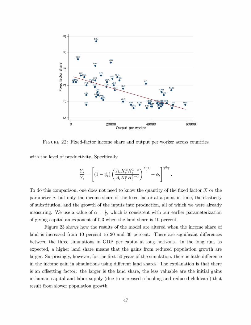
Figure 22: Fixed-factor income share and output per worker across countries

with the level of productivity. Specifically,

YsYt

=

[(1− φt)

(AsK

αsH

1−αs

AtKαt H

1−αt

)σ−1σ

+ φt

] σσ−1

.

To do this comparison, one does not need to know the quantity of the fixed factor X or the

parameter a, but only the income share of the fixed factor at a point in time, the elasticity

of substitution, and the growth of the inputs into production, all of which we were already

measuring. We use a value of α = 13, which is consistent with our earlier parameterization

of giving capital an exponent of 0.3 when the land share is 10 percent.

Figure 23 shows how the results of the model are altered when the income share of

land is increased from 10 percent to 20 and 30 percent. There are significant differences

between the three simulations in GDP per capita at long horizons. In the long run, as

expected, a higher land share means that the gains from reduced population growth are

larger. Surprisingly, however, for the first 50 years of the simulation, there is little difference

in the income gain in simulations using different land shares. The explanation is that there

is an offsetting factor: the larger is the land share, the less valuable are the initial gains

in human capital and labor supply (due to increased schooling and reduced childcare) that

result from slower population growth.

47

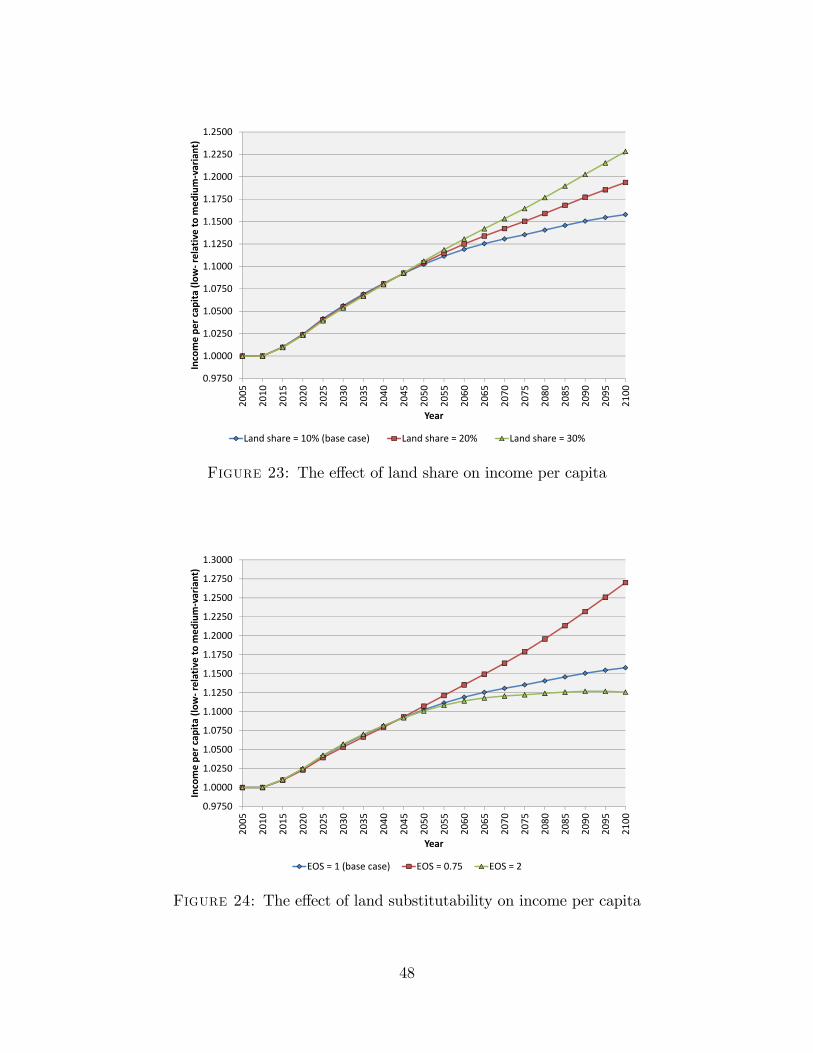
0.9750

1.0000

1.0250

1.0500

1.0750

1.1000

1.1250

1.1500

1.1750

1.2000

1.2250

1.2500

2005

2010

2015

2020

2025

2030

2035

2040

2045

2050

2055

2060

2065

2070

2075

2080

2085

2090

2095

2100

Income pe

r cap

ita (low

‐relative to m

edium‐variant)

Year

Land share = 10% (base case) Land share = 20% Land share = 30%

Figure 23: The effect of land share on income per capita

0.9750

1.0000

1.0250

1.0500

1.0750

1.1000

1.1250

1.1500

1.1750

1.2000

1.2250

1.2500

1.2750

1.3000

2005

2010

2015

2020

2025

2030

2035

2040

2045

2050

2055

2060

2065

2070

2075

2080

2085

2090

2095

2100

Income pe

r cap

ita (low

‐relative to m

edium‐variant)

Year

EOS = 1 (base case) EOS = 0.75 EOS = 2

Figure 24: The effect of land substitutability on income per capita

48

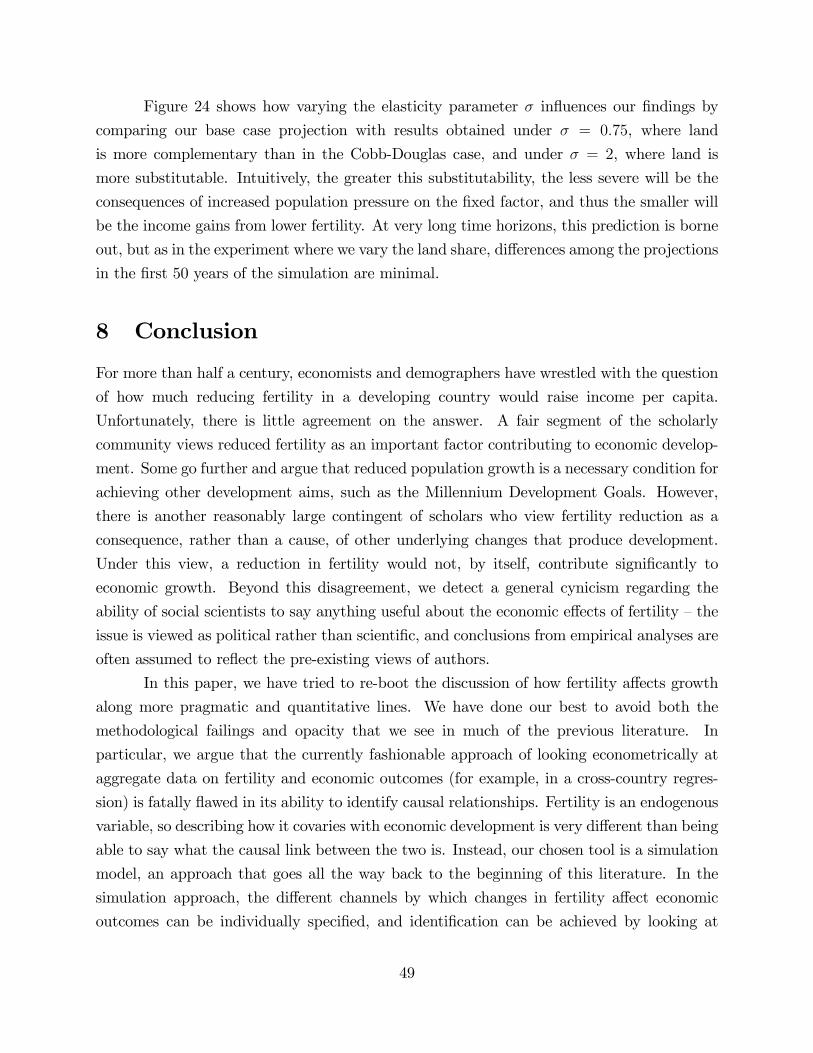
Figure 24 shows how varying the elasticity parameter σ influences our findings by

comparing our base case projection with results obtained under σ = 0.75, where land

is more complementary than in the Cobb-Douglas case, and under σ = 2, where land is

more substitutable. Intuitively, the greater this substitutability, the less severe will be the

consequences of increased population pressure on the fixed factor, and thus the smaller will

be the income gains from lower fertility. At very long time horizons, this prediction is borne

out, but as in the experiment where we vary the land share, differences among the projections

in the first 50 years of the simulation are minimal.

8 Conclusion

For more than half a century, economists and demographers have wrestled with the question

of how much reducing fertility in a developing country would raise income per capita.

Unfortunately, there is little agreement on the answer. A fair segment of the scholarly

community views reduced fertility as an important factor contributing to economic develop-

ment. Some go further and argue that reduced population growth is a necessary condition for

achieving other development aims, such as the Millennium Development Goals. However,

there is another reasonably large contingent of scholars who view fertility reduction as a

consequence, rather than a cause, of other underlying changes that produce development.

Under this view, a reduction in fertility would not, by itself, contribute significantly to

economic growth. Beyond this disagreement, we detect a general cynicism regarding the

ability of social scientists to say anything useful about the economic effects of fertility —the

issue is viewed as political rather than scientific, and conclusions from empirical analyses are

often assumed to reflect the pre-existing views of authors.

In this paper, we have tried to re-boot the discussion of how fertility affects growth

along more pragmatic and quantitative lines. We have done our best to avoid both the

methodological failings and opacity that we see in much of the previous literature. In

particular, we argue that the currently fashionable approach of looking econometrically at

aggregate data on fertility and economic outcomes (for example, in a cross-country regres-

sion) is fatally flawed in its ability to identify causal relationships. Fertility is an endogenous

variable, so describing how it covaries with economic development is very different than being

able to say what the causal link between the two is. Instead, our chosen tool is a simulation

model, an approach that goes all the way back to the beginning of this literature. In the

simulation approach, the different channels by which changes in fertility affect economic

outcomes can be individually specified, and identification can be achieved by looking at

49

microeconomic evidence. In addition to this microeconomic evidence, we bring to bear data

on demographic structure, measures of the natural resource share in national income, and

standard components of quantitative macroeconomic theory. Our simulation exercise is not

meant to deliver the best possible forecast of future GDP, but rather (as is true in any

experimental approach) it takes a ceteris paribus approach, comparing the outcomes in a

country that follows a low fertility path with an otherwise identical country following a higher

fertility path.

We have shown that a simulation model need not be a black box, in which the authors’

prejudices can be comfortably hidden. We deal with the problem of opacity by fully laying

out the model’s structure, and showing robustness to changes in parameters or elimination of

different channels. Further, to a far greater extent than previous authors, we have grounded

the different structural channels in our model on a base of well-specified microeconomic

studies. In this sense, we have incorporated a good deal of literature that is relevant to the

issue of how fertility affects economic growth but does not address that question directly.

Finally, we arm the reader with the ultimate tool for penetrating the black box by providing

a fully working version of our model, in which the user can shut down channels, change

parameters, and alter the demographic scenarios with ease.

An additional advantage of our methodological approach is that we are able to look

not only at the aggregate effect of fertility reduction on income, but also at the different

channels through which this effect operates. This allows us to link our result back to

the underlying theoretical channels that are discussed in the literature. To be specific,

we examine eight different channels: congestion of fixed factors (Malthus effect), capital

shallowing (Solow effect), changes in the ratio of workers to dependents (dependency effect),

changes in the average experience of the population (experience effect), changes in the saving

rate (life-cycle saving effect), changes in the labor supply of working-age adults (life-cycle

labor supply and childcare effects), and changes in the average level of schooling (child-quality

effect). Each channel is separately modeled and parameterized.

A final advantage of our approach is that we have posed the question of how fertility

affects growth in the context of examining the difference between outcomes resulting from

two fully-specified demographic scenarios. One of the many issues that cloud the current

discussion of the economic effects of fertility reduction is that different authors focus on

different fertility reductions. This makes it hard to see the extent to which their predictions

conform with one another. In this paper, we have shown how the findings of our simulation

model could be compared directly to the estimates from a cross-country regression study. We

think that this sort of approach should always be taken in evaluating regression coeffi cients;

50

and similarly that simulation models should be compared by using the same demographic

scenarios.

We apply our simulation model to data fromNigeria. The reduction in fertility that we

consider is the difference between the medium- and low-fertility variants of the UN’s (2010)

population forecasts. This is a difference in the TFR of 0.5, phased in over a period of 15

years, relative to a baseline of declining fertility. This particular reduction seems reasonable

as something that could result from some exogenous intervention. For a base case set of

parameters, we find that this reduction in fertility will raise output per capita by 5.6 percent

at a horizon of 20 years, and by 11.9 percent at a horizon of 50 years. The effects that we

find are roughly linear in the size of the fertility reduction considered —a reduction in the

TFR by one leads to roughly twice as big an increase in output per capita. The dependency

effect, and to a lesser extent the labor supply effects, are the dominant channels by which

reduced fertility affects income per capita in the short run (in the first quarter century after

a fertility reduction). At a horizon of 50 years, the four dominant effects are dependency

(36.7 percent of the total), Solow (22.0 percent), schooling (18 percent) and Malthus (10.4

percent). In the very long run, the Malthus effect becomes the dominant channel, followed

in importance by the Solow effect.

Is the effect of fertility reduction that we find large? To some extent, the answer to

this question depends on what benchmark one is using. NRC (1986) frames the question

as whether a reduction in fertility would be to “vault a typical country into the ranks of

the developed,”and concludes that the answer is definitely “no.”The results presented here

are certainly consistent with this view. But the belief that fertility reduction alone could

be the key to development probably has few adherents today anyway. Authors such as

Das Gupta, Bongaarts, and Cleland (2011) and Sindig (2009) use terms like “important

secondary role” and “necessary condition” in referring to the effect of slowing population

growth on development. Although they do not quantify these terms, our sense is that the

results we find are smaller than what these authors believe. For example, the effect on GDP

per capita that we find, 11.9 percent over 50 years resulting from a TFR reduction of 0.5,

amounts to a change in the growth rate of only about a quarter of a percent per year. By

contrast, between 1990 and 2009, GDP per capita in Nigeria grew at 2.9 percent per year

(although during the two decades prior to that it actually fell slightly).

Another useful benchmark against which one can compare our results is the findings

of cross-country regressions in which the growth rate of income per capita is the dependent

variable and measures of demographic change (such as the growth rate of the working-age

fraction of the population) are on the right hand side. Regressions like these are widely

51

used in policy-oriented discussions of the effects of demographic change. In Section 5 of this

paper, we go through the exercise of applying the findings in one such study, Bloom and

Canning (2008), to the demographic scenarios that we analyze. We find that our estimate

of the economic impact of fertility reduction is roughly twice as large as theirs.

Yet another way to benchmark our results is to look directly at poverty. This seems

natural, given that we are focusing our analysis on poor countries, most of which will likely

still be poor several decades hence. In 2010, the poverty rate in Nigeria was 68 percent. The

World Bank (2000) estimates the elasticity of poverty rates with respect to average income

to be in the neighborhood of two. Thus, the increase of 5.6 percent in income per capita

would reduce the poverty rate by approximately 7.5 percentage points. This seems to us

to be a significant magnitude. Of course, as we have stressed repeatedly, concluding that a

given fertility reduction would have an economically significant effect on income per capita

is very different from concluding that engineering such a fertility reduction would be a good

thing. To address the latter question, one would have to know the costs, both financial

and in terms of welfare, of lowering fertility, and one would also have to have some way of

assessing the utility consequences of children not being born.

Finally, in discussing the magnitude of the results that we present, we want to return

to the issue of methodology. We think that a key advantage of the simulation model we

have presented is its transparency. If one believes that the effects of population on economic

development are larger than what we have estimated, then there has to be a way to alter

our model to produce that larger effect, either by changing the parameters or by introducing

new channels that we have left out. We think that conducting the debate in terms of specific

parameters and channels is likely to be far more enlightening than debating the overall effect

of fertility changes.

52

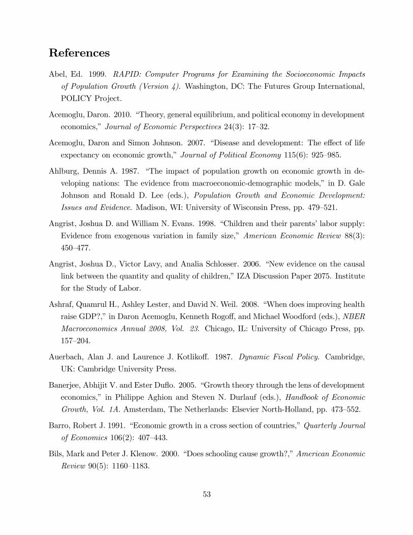
References

Abel, Ed. 1999. RAPID: Computer Programs for Examining the Socioeconomic Impacts

of Population Growth (Version 4). Washington, DC: The Futures Group International,

POLICY Project.

Acemoglu, Daron. 2010. “Theory, general equilibrium, and political economy in development

economics,”Journal of Economic Perspectives 24(3): 17—32.

Acemoglu, Daron and Simon Johnson. 2007. “Disease and development: The effect of life

expectancy on economic growth,”Journal of Political Economy 115(6): 925—985.

Ahlburg, Dennis A. 1987. “The impact of population growth on economic growth in de-

veloping nations: The evidence from macroeconomic-demographic models,” in D. Gale

Johnson and Ronald D. Lee (eds.), Population Growth and Economic Development:

Issues and Evidence. Madison, WI: University of Wisconsin Press, pp. 479—521.

Angrist, Joshua D. and William N. Evans. 1998. “Children and their parents’labor supply:

Evidence from exogenous variation in family size,”American Economic Review 88(3):

450—477.

Angrist, Joshua D., Victor Lavy, and Analia Schlosser. 2006. “New evidence on the causal

link between the quantity and quality of children,”IZA Discussion Paper 2075. Institute

for the Study of Labor.

Ashraf, Quamrul H., Ashley Lester, and David N. Weil. 2008. “When does improving health

raise GDP?,”in Daron Acemoglu, Kenneth Rogoff, and Michael Woodford (eds.), NBER

Macroeconomics Annual 2008, Vol. 23. Chicago, IL: University of Chicago Press, pp.

157—204.

Auerbach, Alan J. and Laurence J. Kotlikoff. 1987. Dynamic Fiscal Policy. Cambridge,

UK: Cambridge University Press.

Banerjee, Abhijit V. and Ester Duflo. 2005. “Growth theory through the lens of development

economics,” in Philippe Aghion and Steven N. Durlauf (eds.), Handbook of Economic

Growth, Vol. 1A. Amsterdam, The Netherlands: Elsevier North-Holland, pp. 473—552.

Barro, Robert J. 1991. “Economic growth in a cross section of countries,”Quarterly Journal

of Economics 106(2): 407—443.

Bils, Mark and Peter J. Klenow. 2000. “Does schooling cause growth?,”American Economic

Review 90(5): 1160—1183.

53

Birdsall, Nancy. 1988. “Economic approaches to population growth,”in Hollis Chenery and

T.N. Srinivasan (eds.), Handbook of Development Economics, Vol. 1. Amsterdam, The

Netherlands: Elsevier North-Holland, pp. 477—542.

Black, Sandra E., Paul J. Devereux, and Kjell G. Salvanes. 2005. “The more the merrier?

The effect of family size and birth order on children’s education,”Quarterly Journal of

Economics 120(2): 669—700.

Bloom, David E. and David Canning. 2008. “Global demographic change: Dimensions and

economic significance,”Population and Development Review 34(Supplement): 17—51.

Bloom, David E., David Canning, Günther Fink, and Jocelyn E. Finlay. 2009. “Fertility,

female labor force participation, and the demographic dividend,”Journal of Economic

Growth 14(2): 79—101.

Bloom, David E. and Jeffrey G. Williamson. 1998. “Demographic transitions and economic

miracles in emerging Asia,”World Bank Economic Review 12(3): 419—455.

Boserup, Ester. 1965. The Conditions of Agricultural Growth: The Economics of Agrarian

Change Under Population Pressure. Chicago, IL: Aldine Publishing.

Brayton, Flint and Peter A. Tinsley. 1996. “A guide to FRB/US: A macroeconomic model

of the United States,”FEDS Working Paper 1996-42. The Board of Governors of the

Federal Reserve System.

Campbell, Martha, John Cleland, Alex Ezeh, and Ndola Prata. 2007. “Return of the

population growth factor,”Science 315(5818): 1501—1502.

Carrasco, Raquel. 2001. “Binary choice with binary endogenous regressors in panel data:

Estimating the effect of fertility on female labor participation,”Journal of Business &

Economic Statistics 19(4): 385—394.

Caselli, Francesco and James Feyrer. 2007. “The marginal product of capital,”Quarterly

Journal of Economics 122(2): 535—568.

Chun, Hyunbae and Jeungil Oh. 2002. “An instrumental variable estimate of the effect of

fertility on the labour force participation of married women,”Applied Economics Letters

9(10): 631—634.

Coale, Ansley J. and Edgar M. Hoover. 1958. Population Growth and Economic Devel-

opment in Low Income Countries: A Case Study of India’s Prospects. Princeton, NJ:

Princeton University Press.

54

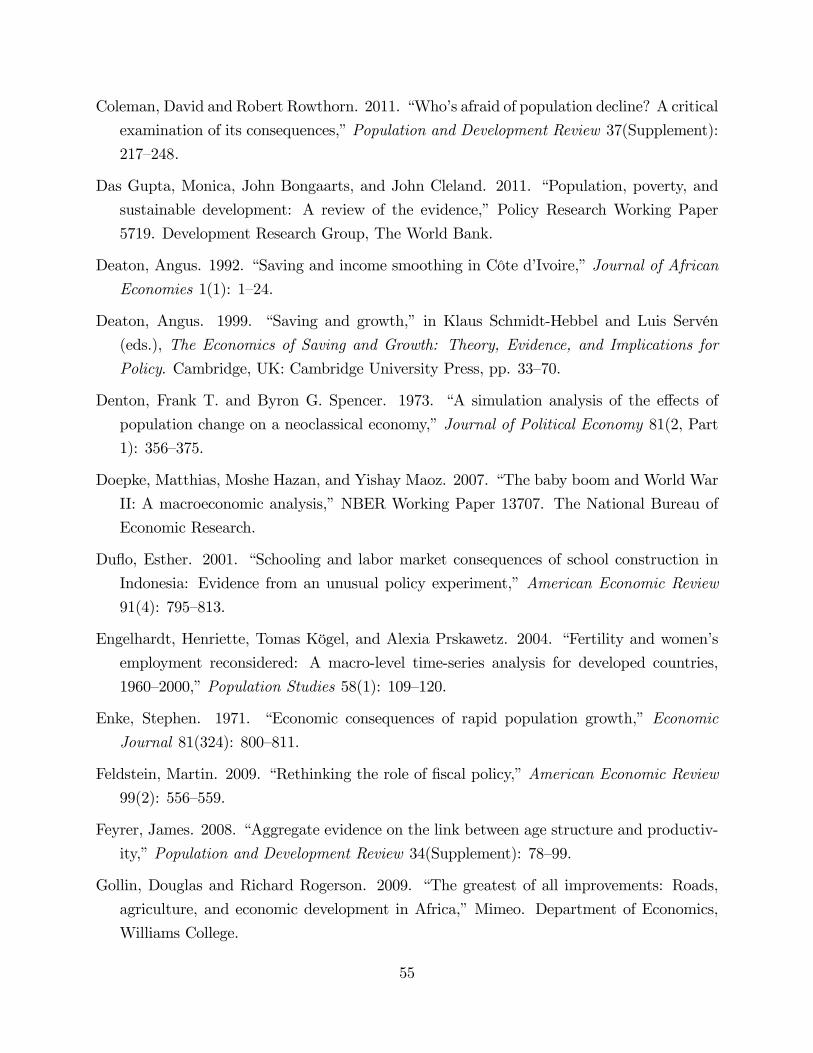
Coleman, David and Robert Rowthorn. 2011. “Who’s afraid of population decline? A critical

examination of its consequences,”Population and Development Review 37(Supplement):

217—248.

Das Gupta, Monica, John Bongaarts, and John Cleland. 2011. “Population, poverty, and

sustainable development: A review of the evidence,” Policy Research Working Paper

5719. Development Research Group, The World Bank.

Deaton, Angus. 1992. “Saving and income smoothing in Côte d’Ivoire,”Journal of African

Economies 1(1): 1—24.

Deaton, Angus. 1999. “Saving and growth,” in Klaus Schmidt-Hebbel and Luis Servén

(eds.), The Economics of Saving and Growth: Theory, Evidence, and Implications for

Policy. Cambridge, UK: Cambridge University Press, pp. 33—70.

Denton, Frank T. and Byron G. Spencer. 1973. “A simulation analysis of the effects of

population change on a neoclassical economy,”Journal of Political Economy 81(2, Part

1): 356—375.

Doepke, Matthias, Moshe Hazan, and Yishay Maoz. 2007. “The baby boom and World War

II: A macroeconomic analysis,”NBER Working Paper 13707. The National Bureau of

Economic Research.

Duflo, Esther. 2001. “Schooling and labor market consequences of school construction in

Indonesia: Evidence from an unusual policy experiment,”American Economic Review

91(4): 795—813.

Engelhardt, Henriette, Tomas Kögel, and Alexia Prskawetz. 2004. “Fertility and women’s

employment reconsidered: A macro-level time-series analysis for developed countries,

1960—2000,”Population Studies 58(1): 109—120.

Enke, Stephen. 1971. “Economic consequences of rapid population growth,” Economic

Journal 81(324): 800—811.

Feldstein, Martin. 2009. “Rethinking the role of fiscal policy,”American Economic Review

99(2): 556—559.

Feyrer, James. 2008. “Aggregate evidence on the link between age structure and productiv-

ity,”Population and Development Review 34(Supplement): 78—99.

Gollin, Douglas and Richard Rogerson. 2009. “The greatest of all improvements: Roads,

agriculture, and economic development in Africa,”Mimeo. Department of Economics,

Williams College.

55

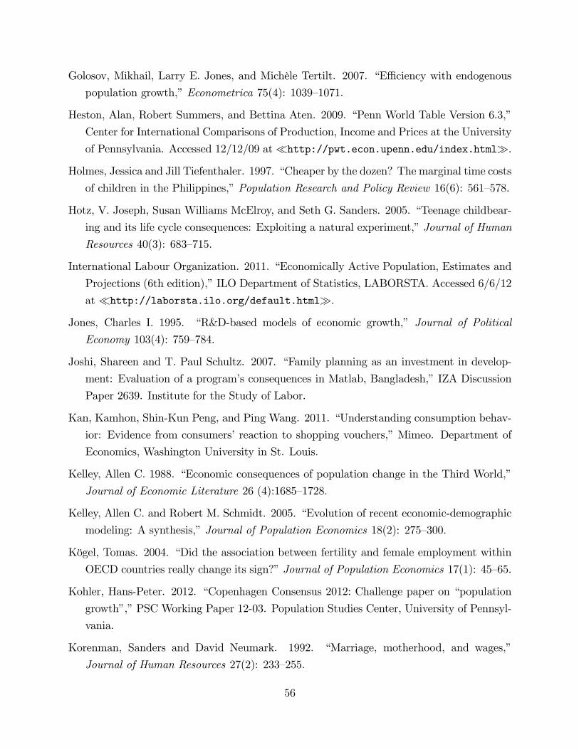
Golosov, Mikhail, Larry E. Jones, and Michèle Tertilt. 2007. “Effi ciency with endogenous

population growth,”Econometrica 75(4): 1039—1071.

Heston, Alan, Robert Summers, and Bettina Aten. 2009. “Penn World Table Version 6.3,”

Center for International Comparisons of Production, Income and Prices at the University

of Pennsylvania. Accessed 12/12/09 at�http://pwt.econ.upenn.edu/index.html�.

Holmes, Jessica and Jill Tiefenthaler. 1997. “Cheaper by the dozen? The marginal time costs

of children in the Philippines,”Population Research and Policy Review 16(6): 561—578.

Hotz, V. Joseph, Susan Williams McElroy, and Seth G. Sanders. 2005. “Teenage childbear-

ing and its life cycle consequences: Exploiting a natural experiment,”Journal of Human

Resources 40(3): 683—715.

International Labour Organization. 2011. “Economically Active Population, Estimates and

Projections (6th edition),”ILO Department of Statistics, LABORSTA. Accessed 6/6/12

at �http://laborsta.ilo.org/default.html�.

Jones, Charles I. 1995. “R&D-based models of economic growth,” Journal of Political

Economy 103(4): 759—784.

Joshi, Shareen and T. Paul Schultz. 2007. “Family planning as an investment in develop-

ment: Evaluation of a program’s consequences in Matlab, Bangladesh,”IZA Discussion

Paper 2639. Institute for the Study of Labor.

Kan, Kamhon, Shin-Kun Peng, and Ping Wang. 2011. “Understanding consumption behav-

ior: Evidence from consumers’reaction to shopping vouchers,”Mimeo. Department of

Economics, Washington University in St. Louis.

Kelley, Allen C. 1988. “Economic consequences of population change in the Third World,”

Journal of Economic Literature 26 (4):1685—1728.

Kelley, Allen C. and Robert M. Schmidt. 2005. “Evolution of recent economic-demographic

modeling: A synthesis,”Journal of Population Economics 18(2): 275—300.

Kögel, Tomas. 2004. “Did the association between fertility and female employment within

OECD countries really change its sign?”Journal of Population Economics 17(1): 45—65.

Kohler, Hans-Peter. 2012. “Copenhagen Consensus 2012: Challenge paper on “population

growth”,”PSC Working Paper 12-03. Population Studies Center, University of Pennsyl-

vania.

Korenman, Sanders and David Neumark. 1992. “Marriage, motherhood, and wages,”

Journal of Human Resources 27(2): 233—255.

56

Kuznets, Simon. 1967. “Population and economic growth,”Proceedings of the American

Philosophical Society 111(3): 170—193.

Lee, Jungmin. 2008. “Sibling size and investment in children’s education: An Asian

instrument,”Journal of Population Economics 21(4): 855—875.

Lee, Ronald. 1980. “Age structure, intergenerational transfers and economic growth: An

overview,”Revue économique 31(6): 1129—1156.

Lee, Ronald and Andrew Mason. 2010. “Some macroeconomic aspects of global population

aging,”Demography 47(Supplement): S151—S172.

Lee, Ronald and Andrew Mason. 2011. Population Aging and the Generational Economy:

A Global Perspective. Cheltenham, UK: Edward Elgar.

Lee, Roland D., Andrew Mason, and Tim Miller. 2001. “Saving, wealth, and population,”

in Nancy Birdsall, Allen C. Kelley, and Steven W. Sindig (eds.), Population Matters:

Demographic Change, Economic Growth, and Poverty in the Developing World. New

York, NY: Oxford University Press, pp. 137—164.

Li, Hongbin and Junsen Zhang. 2007. “Do high birth rates hamper economic growth?”

Review of Economics and Statistics 89(1): 110—117.

Lim, Kyung-Mook and David N. Weil. 2003. “The baby boom and the stock market boom,”

Scandinavian Journal of Economics 105(3): 359—377.

Malthus, Thomas R. 1798. An Essay on the Principle of Population. Reprint 2004. Edited

with an introduction and notes by Geoffrey Gilbert. Oxford, UK: Oxford University

Press.

Mankiw, N. Gregory, David Romer, and David N. Weil. 1992. “A contribution to the

empirics of economic growth,”Quarterly Journal of Economics 107(2): 407—437.

McNown, Robert and Sameer Rajbhandary. 2003. “Time series analysis of fertility and female

labor market behavior,”Journal of Population Economics 16(3): 501—523.

Miller, Grant. 2010. “Contraception as development? New evidence from family planning

in Colombia,”Economic Journal 120(545): 709—736.

Mincer, Jacob. 1974. Schooling, Experience, and Earnings. New York, NY: Columbia

University Press (for NBER).

National Academy of Sciences. 1971. Rapid Population Growth: Consequences and Policy

Implications. Baltimore, MD: Johns Hopkins Press.

57

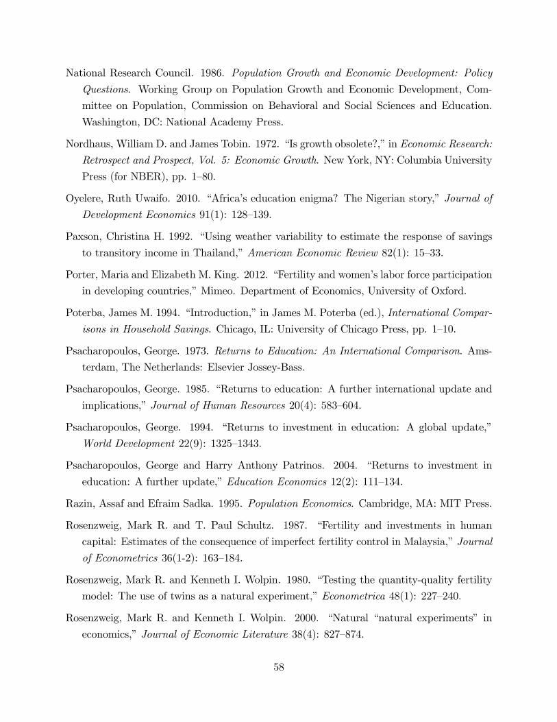
National Research Council. 1986. Population Growth and Economic Development: Policy

Questions. Working Group on Population Growth and Economic Development, Com-

mittee on Population, Commission on Behavioral and Social Sciences and Education.

Washington, DC: National Academy Press.

Nordhaus, William D. and James Tobin. 1972. “Is growth obsolete?,”in Economic Research:

Retrospect and Prospect, Vol. 5: Economic Growth. New York, NY: Columbia University

Press (for NBER), pp. 1—80.

Oyelere, Ruth Uwaifo. 2010. “Africa’s education enigma? The Nigerian story,”Journal of

Development Economics 91(1): 128—139.

Paxson, Christina H. 1992. “Using weather variability to estimate the response of savings

to transitory income in Thailand,”American Economic Review 82(1): 15—33.

Porter, Maria and Elizabeth M. King. 2012. “Fertility and women’s labor force participation

in developing countries,”Mimeo. Department of Economics, University of Oxford.

Poterba, James M. 1994. “Introduction,”in James M. Poterba (ed.), International Compar-

isons in Household Savings. Chicago, IL: University of Chicago Press, pp. 1—10.

Psacharopoulos, George. 1973. Returns to Education: An International Comparison. Ams-

terdam, The Netherlands: Elsevier Jossey-Bass.

Psacharopoulos, George. 1985. “Returns to education: A further international update and

implications,”Journal of Human Resources 20(4): 583—604.

Psacharopoulos, George. 1994. “Returns to investment in education: A global update,”

World Development 22(9): 1325—1343.

Psacharopoulos, George and Harry Anthony Patrinos. 2004. “Returns to investment in

education: A further update,”Education Economics 12(2): 111—134.

Razin, Assaf and Efraim Sadka. 1995. Population Economics. Cambridge, MA: MIT Press.

Rosenzweig, Mark R. and T. Paul Schultz. 1987. “Fertility and investments in human

capital: Estimates of the consequence of imperfect fertility control in Malaysia,”Journal

of Econometrics 36(1-2): 163—184.

Rosenzweig, Mark R. and Kenneth I. Wolpin. 1980. “Testing the quantity-quality fertility

model: The use of twins as a natural experiment,”Econometrica 48(1): 227—240.

Rosenzweig, Mark R. and Kenneth I. Wolpin. 2000. “Natural “natural experiments” in

economics,”Journal of Economic Literature 38(4): 827—874.

58

Rosenzweig, Mark R. and Junsen Zhang. 2009. “Do population control policies induce more

human capital investment? Twins, birth weight and China’s “one-child”policy,”Review

of Economic Studies 76(3): 1149—1174.

Sanderson, Warren. 2004. “The SEDIM model: Version 1.0,” Interim Report IR-04-041.

International Institute for Applied Systems Analysis.

Schultz, T. Paul. 2004. “Evidence of returns to schooling in Africa from household surveys:

Monitoring and restructuring the market for education,”Journal of African Economies

13(Supplement): ii95—ii148.

Schultz, T. Paul. 2009. “How does family planning promote development? Evidence from a

social experiment in Matlab, Bangladesh, 1977-1996,”Mimeo. Department of Economics,

Yale University.

Simon, Julian L. 1976. “Population growth may be good for LDCs in the long run: A richer

simulation model,”Economic Development and Cultural Change 24(2): 309—337.

Sindig, Steven W. 2009. “Population, poverty and economic development,”Philosophical

Transactions of the Royal Society B, 364(1532): 3023—3030.

Solow, Robert M. 1956. “A contribution to the theory of economic growth,” Quarterly

Journal of Economics 70(1): 65—94.

Soyibo, Adedoyin, Olanrewaju Olaniyan, and Akanni O. Lawanson. 2011. “The structure of

generational public transfer flows in Nigeria,”in Ronald Lee and Andrew Mason (eds.),

Population Aging and the Generational Economy: A Global Perspective. Cheltenham,

UK: Edward Elgar.

Tiefenthaler, Jill. 1997. “Fertility and family time allocation in the Philippines,”Population

and Development Review 23(2): 377—397.

Troske, Kenneth R. and Alexandru Voicu. 2010. “Joint estimation of sequential labor force

participation and fertility decisions using Markov chain Monte Carlo techniques,”Labour

Economics 17(1): 150—169.

United Nations. 2010. “World Population Prospects: The 2010 Revision,”Department of

Economic and Social Affairs, Population Division, Population Estimates and Projections

Section. Accessed 6/4/12 at �http://esa.un.org/unpd/wpp/index.htm�.

Weil, David N. 1994. “The saving of the elderly in micro and macro data,”Quarterly Journalof Economics 109(1): 55—81.

59

Weil, David N. 2008a. “Rapid population growth raises the stakes for African governments,”

in Africa’s Turn?. Boston, MA: Boston Review Books, MIT Press, pp. 79—90.

Weil, David N. 2008b. “Population aging,” in Steven N. Durlauf and Lawrence E. Blume

(eds.), The New Palgrave Dictionary of Economics, 2nd edition. New York, NY: Palgrave

Macmillan.

Weil, David N. and Joshua Wilde. 2009. “How relevant is Malthus for economic development

today?”American Economic Review 99(2): 255—260.

World Bank. 2000. World Development Report 2000/2001: Attacking Poverty. New York,

NY: Oxford University Press.

World Bank. 2005. Where Is the Wealth of Nations? Measuring Capital for the 21st Century.

Washington, DC: World Bank.

Young, Alwyn. 2005. “The gift of the dying: The tragedy of AIDS and the welfare of future

African generations,”Quarterly Journal of Economics 120(2): 423—466.

60