1

Discrete Element Modelling and Cavity Expansion Analysis

of Cone Penetration Testing

O. Falagush, G. R. McDowell*, H. S. Yu, J. P. de Bono

* Corresponding Author: Glenn.McDowell@nottingham.ac.uk

Abstract This paper uses the discrete element method (DEM) in three dimensions to simulate cone

penetration testing (CPT) of granular materials in a calibration chamber. Several researchers

have used different numerical techniques such as strain path methods and finite element

methods to study CPT problems. The DEM is a useful alternative tool for studying cone

penetration problems because of its ability to provide micro mechanical insight into the

behaviour of granular materials and cone penetration resistance. A 30° chamber segment and a

particle refinement method were used for the simulations. Giving constant mass to each particle

in the sample was found to reduce computational time significantly, without significantly

affecting tip resistance. The effects of initial sample conditions and particle friction coefficient

on tip resistance are investigated and found to have an important effect on the tip resistance.

Biaxial test simulations using DEM are conducted to obtain the basic granular material

properties for obtaining CPT analytical solutions based on continuum mechanics. Macro

properties of the samples for different input micro parameters are presented and used to obtain

the analytical CPT results. Comparison between the numerical simulations and analytical

solutions show good agreement.

1 Introduction Cone penetration testing (CPT) is one of the most versatile devices for in-situ soil testing. With

minimal disturbance to the ground, it provides information about soil classification and

geotechnical parameters. Interpretation of CPT results in sand relies mainly on empirical

correlations [1]. Different correlations have been developed from tests in calibration chambers,

where the sample can be consolidated to a desired stress level and boundary conditions can be

accurately controlled [2–4].

Researchers have used various numerical techniques to study CPT problems; for example Susila

and Hryciw [5] used finite element modelling to simulate CPTs in normally consolidated sand,

and their results showed some excellent agreement with earlier analytical and experimental

studies. Ahmadi et al [6] also estimated cone tip resistance in sand using the finite difference

method, and found the error band between predicted and measured values from the calibration

chamber to be ±25%.

The Discrete Element Method (DEM) is a useful tool for studying CPT in granular materials as it

gives an alternative approach to current large-displacement finite-element models and can

provide micro-mechanical insight into this important boundary value problem. Huang and

2

Ma [7], Calvetti et al. [8] and Jiang et al. [9] all used two-dimensional DEM simulations to study

cone penetration tests. Although qualitative insight was obtained, the limitations of their disc-

based models excluded quantitative comparisons with physical tests. Moreover, the kinematic

constraints of two-dimensional simulations are substantially different from three-dimensional

(3D) simulations and real granular material.

Arroyo et al. [10] used a 3D DEM model of a virtual calibration chamber to simulate cone

penetration tests in sand using spheres with prohibited rotation. Their results were compared

to experimental tests conducted in Ticino sand by Jamiolkowski et al. [11]. The particles used in

their model were scaled to 50 times larger than the Ticino sand. A small cubical numerical

sample (of size 8 mm) was used to calibrate the material parameters, Arroyo et al. [10]

determined these parameters by trial and error in order to provide a best fit to a single set of

data for a drained isotropic compression test. Their numerical results under isotropic boundary

stresses showed good quantitative agreement with the predictions of the empirical equations

based on the physical results. However, particle size scaling is not recommended as it decreases

the ratio between cone diameter and d50, the median particle size (B ⁄ d50), thereby decreasing

the number of particles in contact with the cone tip and creating large voids around it. The

agreement demonstrated between DEM and experimental results can be attributed to the

prohibition of particle rotation.

In this paper a particle refinement method [12] is implemented to simulate CPT in a 30°

segment of a calibration chamber. In order to improve the computational efficiency of the

simulations, the radius expansion method is used to generate the sample, and constant particle

mass (i.e. particles of all sizes have the same mass) is implemented throughout the simulations.

Results are presented for a series of cone penetration tests in which a brief summary of the

effects of micro parameters (such as particle friction and porosity) on the tip resistance is given.

Biaxial tests are then performed on the same material, to obtain the macroscopic soil

characteristics. These are then used to obtain an analytical solution for the tip resistance, qc,

using cavity-expansion theory [13, 14], which is compared to the numerical results.

2 Cone Penetration Test Simulations

2.1 Modelling Procedure and Sample Preparation

In the authors’ previous work [15] a 90° segment of a calibration chamber was considered in

order to enable smaller particles to be modelled without excessive computation time. They also

reduced the chamber height H and width Dc. The use of smaller particles provided a more

realistic ratio of cone diameter to median particle diameter (B ⁄ d50) and ensured that during

penetration, the cone tip remained in contact with an acceptable number of particles. Their

results showed that using a chamber height of 100 mm and a width of 300 mm gave an

acceptable computational time without significantly affecting the measured tip resistance. The

experimental results of Schnaid [16] for Leighton Buzzard sand was used as a benchmark for

comparison with the numerical model and to establish the suitability of the model parameters.

In order to obtain a larger number of small particles in contact with the cone tip, the authors’

subsequently used a ‘particle refinement method’ [12], whereby small particles were generated

close to the cone penetrometer, and larger particles further away. They simulated sand particles

of size 1.5 mm near the cone penetrometer, using both 90° and 30° segments of the calibration

3

chamber. They showed that using a sample comprising three different particle sizes minimised

the computational time while effectively giving the same resistance as using a sample

comprising only single-sized particles. In addition, they showed that to simulate a sand-sized

particle of 1.5 mm or 2.0 mm near the cone penetrometer, a 30° segment of the calibration

chamber can be used instead of a 90° segment (which requires an impractical number of

particles).

Although an alternative method could be to use periodic boundaries, which may help minimise

boundaries effects close to the cone, this would add additional computational weight to the

simulations. As one of the aims of this paper is to investigate how the efficiency of the authors’

previous model could be improved, it was chosen to use fixed boundaries, also maintaining

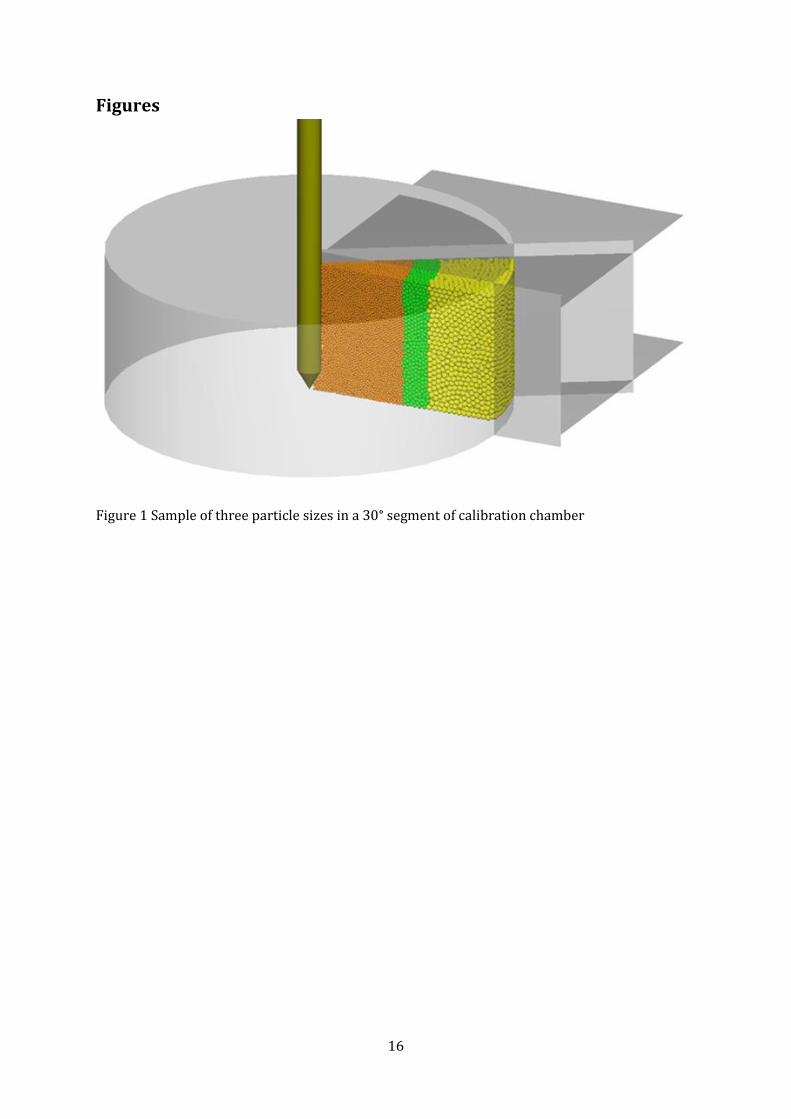
consistency with previous work. As such, the model used in this study comprises a refined

sample of spheres simulated in a 30° segment of a calibration chamber, shown in Figure 1. The

samples used consist of a minimum of three zones of different-sized particles; the difference in

particle size between any neighbouring zones is chosen so as to prevent excessive migration of

the smaller particles into the larger voids [12]. The numerical chamber comprises five finite

frictionless walls that serve as sample boundaries to confine the particles during sample

generation and equilibrium (outer cylindrical wall, two vertical planar walls at 30° to each

other, top and bottom planar walls). The use of frictionless walls was chosen to minimise the

boundary effects from the lateral chamber wall. Additional, temporary frictionless walls are

used as interfaces between the particles zones to separate them during the sample preparation

process. Table 1 shows the dimensions and boundary conditions of both the experimental

results from Schnaid [16] and the optimal numerical calibration chamber. Although this work

(as well as the previous) uses spheres (which lack interlocking and can be considered

unrealistic) readers are directed to [17] for related work that focuses on investigating both the

effects of particle shape and crushing during CPT using DEM. It should be noted that the

objective of this paper is not an attempt to model a single specific piece of data for a specific soil,

but further confirm the suitability of simulating CPT using a realistic cone size with DEM in an

aggregate comprising sand-sized grains, to investigate methods of improving simulation time

and further explore the effects of various micro parameters on the macroscopic behaviour of

granular material, and most significantly, compare the results with solutions using cavity

expansion theory.

In the previous work by the authors, the sample was generated using a deposition and

compaction method [15]. This involved creating the spheres in a taller segment and allowing

them to fall under gravity. The software used is PFC3D version 3.1 [18]; the computer used had

an Intel Core Quad CPU (3 GHz) and 3 GB RAM. To reduce the time required for CPT simulations,

the radius expansion method [18] is used here. This method involves creating the particles

randomly within the defined boundaries, at a greatly reduced size, then gradually expanding

them to their final radii. The linear-spring contact model is used for efficiency and simplicity, as

well as for the sake of comparison with earlier work; the particles are given normal and shear

stiffnesses of 5 x 105 N/m. Although a Hertzian contact law would be more realistic, again the

readers are reminded that this is more of a fundamental study than a specific calibration, and

aims to provide a step towards more realistic and complex models. The linear spring contact

model uses the assigned normal stiffness to relate the total normal displacement to the total

normal force acting on a particle, while the shear stiffness relates the increment of shear

4

displacement to the increment of shear force acting on a particle. As well as the software

documentation [18], further details can be found in [19].

Following sample generation, an isotropic compressive stress is then applied by adjusting the

outer cylindrical wall and the bottom wall using a servo-control mechanism. This is maintained

during the cone penetration, and the stresses on all walls are monitored, and are consistent

with the applied stresses before and during penetration). The simulations here all use a 60°

cone penetrometer, of diameter B = 18 mm. A frictional conical wall is used to simulate the tip, a

frictional cylindrical wall is used for the lower sleeve, and a frictionless cylindrical wall is used

for the upper sleeve, as shown in Figure 2. The penetrometer moves with a velocity of 20 mm/s,

the standard value used in experiments [20]. In previous work, it was shown that changing this

value had no influence on the results, and although time cannot be considered real in the

simulations using constant mass, the results show consistency with previous results in which

time was real. Table 2 shows the particle and wall properties for the calibration chamber and

cone penetrometer, which applies to all the simulations presented here (unless stated

otherwise).

2.2 CPT Results

2.2.1 Effects of Sample Preparation Method

To highlight the effects of using the radius expansion method on the preparation time as well as

the tip resistance, two samples were prepared, one using the deposition and compaction

method (simulation A), the other using the radius expansion method (simulation B). Both

samples comprised the identical particle configuration of 2, 3 and 4 mm spheres (as seen in

Figure 1), and have the same wall and particle properties. The chamber inner-segment (75 mm,

radially) next to the cone was filled with 2 mm particles followed by a 20 mm thick band of 3

mm particles, the remaining 55 mm was filled with 4 mm particles. The two samples had the

same initial porosity of 0.37, and were subjected to an isotropic stress of 300 kPa. The porosity

is the same in every zone for both samples. The particle friction coefficient for each of the two

samples was set to 0.5 after isotropic compaction was completed and before pushing the cone.

Figure 3 shows that the ultimate tip resistance for the two simulations to be almost the same,

approximately 7 MPa. The overall simulation time for the simulation (including preparation)

using the radius expansion method was substantially less than the simulation using the

deposition and compaction method, approximately 7 days compared to 30 days, respectively,

illustrating the usefulness of the radius expansion method.

2.2.2 Constant Particle Mass

The use of constant mass was considered due to the need to use even smaller particles in the

vicinity of the cone penetrometer, thereby increasing the number of particles in contact with the

cone tip. The numerical time step used in the software is a function of the particle mass, and

reducing the particle size at constant specific gravity next to the cone reduces the time step,

meaning that the smallest particle size controls the time step and can lead to computational

inefficiency. Therefore, the use of constant particle mass was considered with the aim of

reducing simulation time, given that the simulations were quasi-static in nature, and gravity

was not important under the boundary stresses applied here. Further details on scaling the

timestep and/or density can be found in the software documentation [18].

5

The effects of using constant mass on calculation time and tip resistance are demonstrated by

comparing two simulations (both of which are generated using the radius expansion method),

one with varied particle mass (i.e. constant density—simulation B), and one with constant

particle mass (simulation C). Both samples have the same 2, 3 and 4 mm sphere arrangement

and initial porosity of 0.37. They were subjected to an isotropic compressive stress of 300 kPa.

The results of the two simulations showed almost equal ultimate tip resistances of about 7 MPa

as seen in Figure 4. The simulation using particles with constant density required

approximately 7 days to complete, whereas the simulation using particles of constant mass

needed only 3. It can be deduced from Figure 4 that using particles of constant mass had almost

no effect on the tip resistance compared with particles of constant density. Therefore, a

simulation comprising five particle zones, with diameters 1.0, 1.5, 2.0, 3.0 and 4.0 mm, with

constant mass was performed (simulation D), with the aim of introducing even smaller particles

in the vicinity of the cone. The first zone had a radial distance of 20 mm, the middle three zones

were each 15 mm, and the remaining 85 mm comprised the last zone (filled with 4 mm

particles). As before, the sample has an initial porosity of 0.37 and is subjected to an isotropic

compressive stress of 300 kPa. The number of 1 mm particles in contact with the cone tip was

typically around 52 during the simulation, whereas previously, using 2 mm particles, only

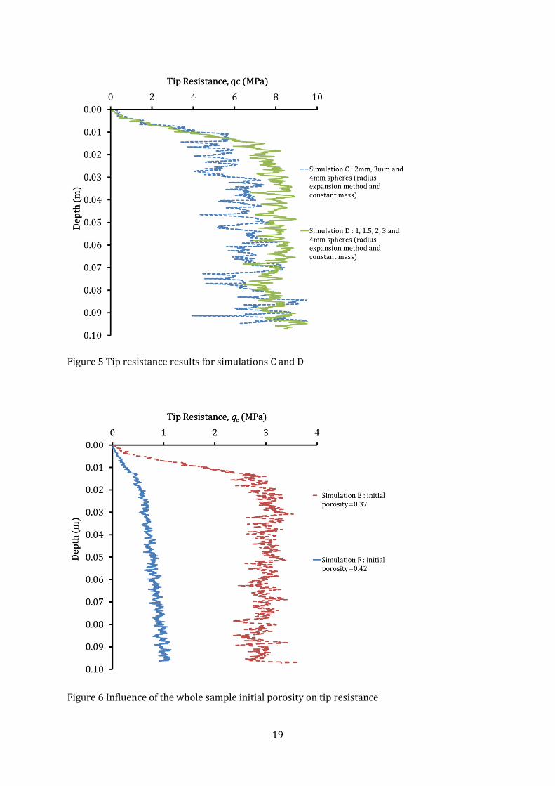
around 14 particles were in contact. Figure 5 compares the tip resistances of simulation C with

simulation D, and it can be seen that the tip resistance for simulation D is higher than that of

simulation C, especially at shallower depths. In addition, using the smaller particles next to the

cone leads to smaller fluctuations in the tip resistance, due to the larger, more reaslistic number

of contacts, which is desirable for CPT modelling in sand and making comparisons with

available data [16].

2.2.3 Initial Porosity

Many researchers have shown that cone tip resistance is significantly affected by initial sample

porosity and mean effective stress [21–24]. To investigate the effect of initial sample porosity on

the measured tip resistance, two simulations (E and F) are presented in Figure 6 which have

alternative particle friction coefficients of 0 and 0.5 respectively during sample preparation and

compaction to 100 kPa, resulting in porosities 0.37 and 0.42 respectively before penetration.

The friction coefficient for the first sample was reset to 0.5 after isotropic compaction was

completed and before pushing the cone. Both samples were then subjected to an isotropic stress

of 100 kPa. The influence of varying initial porosity on cone tip resistance can be seen in Figure

6, where it is evident from comparison that a reduction in the initial porosity leads to an

increase in ultimate tip resistance. The ultimate tip resistance reduces from 3 MPa for the

sample with initial porosity 0.37 to about 1 MPa for the sample with initial porosity 0.42.

2.2.4 Mean Effective Stress

To examine the effect of mean effective stress on the tip resistance results, three simulations

comprising samples with the same initial porosity of 0.37 but varying mean effective stresses

100, 200 and 300 kPa (E, G and D, respectively) were performed. Figure 7 shows that increasing

the mean effective stresses results in progressively larger values of ultimate tip resistance.

Whereas the ultimate tip resistance was about 3 MPa when the mean effective stress was

100 kPa, this value increases to about 6 MPa for a mean effective stress of 200 kPa, and to about

8.5 MPa when the mean effective stress is 300 kPa. It should be noted that for the three

simulations the tip resistance normalised by their initial horizontal stress, qc ⁄ σh, gives

6

approximately the same value of approximately 30, as seen in Figure 8. This value is

approximately 7 times lower if compared with experimental data of Schnaid [16] for dense

Leighton Buzzard sand (of 89% relative density) having an isotropic stress of 100 kPa.

However, it was found that this experimental result is approximately in agreement with

simulation results when particle rotation is prohibited [19].

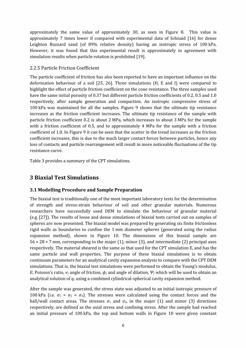
2.2.5 Particle Friction Coefficient

The particle coefficient of friction has also been reported to have an important influence on the

deformation behaviour of a soil [25, 26]. Three simulations (H, E and I) were compared to

highlight the effect of particle friction coefficient on the cone resistance. The three samples used

have the same initial porosity of 0.37 but different particle friction coefficients of 0.2, 0.5 and 1.0

respectively, after sample generation and compaction. An isotropic compressive stress of

100 kPa was maintained for all the samples. Figure 9 shows that the ultimate tip resistance

increases as the friction coefficient increases. The ultimate tip resistance of the sample with

particle friction coefficient 0.2 is about 2 MPa, which increases to about 3 MPa for the sample

with a friction coefficient of 0.5, and to approximately 4 MPa for the sample with a friction

coefficient of 1.0. In Figure 9 it can be seen that the scatter in the trend increases as the friction

coefficient increases, this is due to the much larger contact forces between particles, hence any

loss of contacts and particle rearrangement will result in more noticeable fluctuations of the tip

resistance curve.

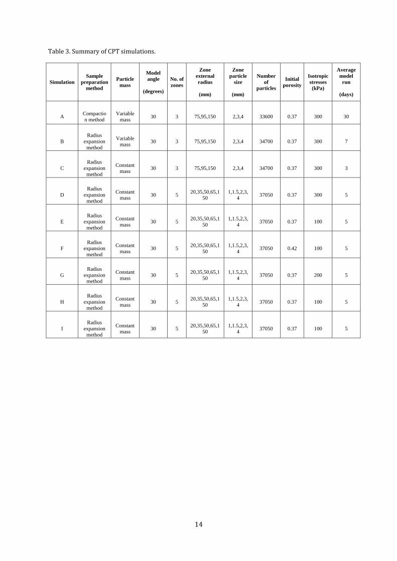
Table 3 provides a summary of the CPT simulations.

3 Biaxial Test Simulations

3.1 Modelling Procedure and Sample Preparation

The biaxial test is traditionally one of the most important laboratory tests for the determination

of strength and stress-strain behaviour of soil and other granular materials. Numerous

researchers have successfully used DEM to simulate the behaviour of granular material

(e.g. [27]). The results of loose and dense simulations of biaxial tests carried out on samples of

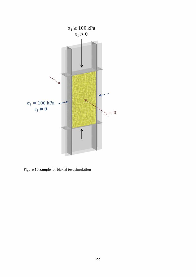
spheres are now presented. The biaxial model was prepared by generating six finite frictionless

rigid walls as boundaries to confine the 1 mm diameter spheres (generated using the radius

expansion method), shown in Figure 10. The dimensions of this biaxial sample are

56 × 28 × 7 mm, corresponding to the major (1), minor (3), and intermediate (2) principal axes

respectively. The material sheared is the same as that used for the CPT simulation E, and has the

same particle and wall properties. The purpose of these biaxial simulations is to obtain

continuum parameters for an analytical cavity expansion analysis to compare with the CPT DEM

simulations. That is, the biaxial test simulations were performed to obtain the Young’s modulus,

E; Poisson’s ratio, ν; angle of friction, ϕ; and angle of dilation, Ψ; which will be used to obtain an

analytical solution of qc using a combined cylindrical-spherical cavity expansion method.

After the sample was generated, the stress state was adjusted to an initial isotropic pressure of

100 kPa (i.e. σ1 = σ2 = σ3). The stresses were calculated using the contact forces and the

ball/wall contact areas. The stresses σ1 and σ3, in the major (1) and minor (3) directions

respectively, are defined as the axial stress and confining stress. After the sample had reached

an initial pressure of 100 kPa, the top and bottom walls in Figure 10 were given constant

7

velocities of 0.01 m/s, while the lateral walls (y-direction) were controlled automatically by a

servo-mechanism to maintain a constant confining stress. The front and back walls in the figure

(z-direction) did not move and were maintained in fixed positions.

3.2 Biaxial Test Results

Two simulations were carried out on two samples with different initial porosities to investigate

the mechanical behaviour of a granular assembly sheared under biaxial conditions. The

porosities of the two samples were 0.37 (dense sample) and 0.42 (loose sample) respectively.

Each sample comprised approximately 13400 spheres, of 1 mm diameter (the size of spheres

next to the cone in the most accurate DEM simulations), shown in Figure 10. The number of

particles was chosen to ensure a reasonable computational time.

The effect of varying porosity on the mechanical behaviour of the granular material for the two

simulations is shown in Figure 11. In Figure 11(a) the peak axial stress achieved for the dense

sample is about 310 kPa at an axial strain of about 2%; the ultimate stress is approximately

225 kPa. The maximum stress reached for the loose sample, at approximately 15% strain, is also

225 kPa. As there is no pore pressure, all stresses can be considered as effective (σ’ = σ). The

maximum angle of friction, ϕ’peak for the plane-strain condition was calculated from the peak

stresses using a Mohr circle of stress as:

sin 𝜙𝑝𝑒𝑎𝑘

′ = 𝜎1

′ − 𝜎3′

𝜎1′ + 𝜎3

′ (1)

and was found to be approximately 32o for the dense sample. The ultimate angle of friction for

both samples was found to be 22o. The plot of volumetric strain against axial strain, in

Figure 11(b) shows that peak strength is related to the maximum rate of dilation. The dense

sample had a maximum dilation angle, ψmax, at peak strength of approximately 15°, compared

with 0° for the loose sample. Both simulations reach constant volume beyond about 15% axial

strain, indicating that critical states are achieved. The maximum dilation angle was calculated

from the strain increments as:

sin 𝛹𝑚𝑎𝑥 =

𝛿휀1 + 𝛿휀3

𝛿휀1 − 𝛿휀3=

𝛿휀v

2𝛿휀1 − 𝛿휀v (2)

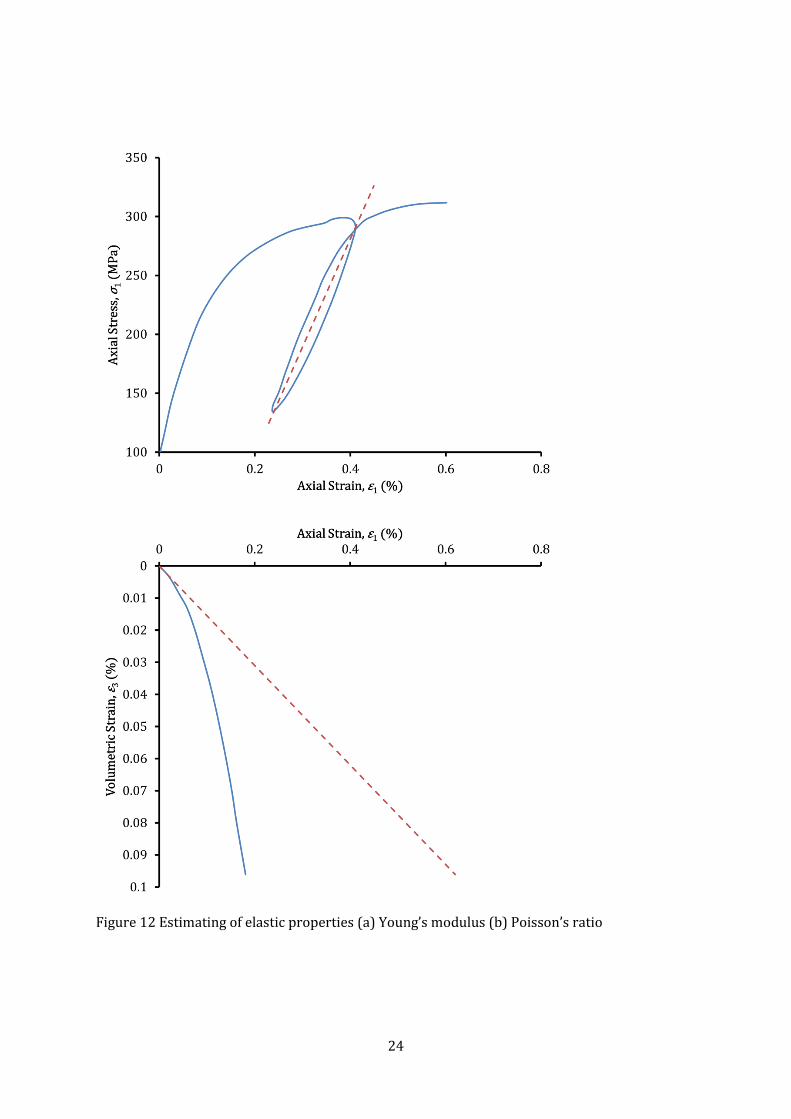
Other parameters obtained from these biaxial tests are the Young’s modulus, E, and the Poisson

ratio, ν. The modulus E was estimated from unload-reload curves obtained from the biaxial test

simulations, to eliminate the effects of particle disturbance; while the Poisson ratio was

estimated from the initial strain curve (example for the dense sample given in Figure 12).

Young’s moduli of E = 62 MPa and 20 MPa, and Poisson ratios of ν = 0.2 were found for the

dense and loose specimens respectively.

These biaxial tests were performed to obtain the material properties required to obtain an

analytical solution for qc using a combined cylindrical-spherical cavity expansion. This paper

will now focus on the comparison between the analytical solution and DEM simulation results

for the cone penetration test.

8

4 Analytical Solution for CPT using Cavity Expansion Method

4.1 Cylindrical-Spherical Cavity Expansion

The similarity between cavity expansion and cone penetration was firstly reported by

Bishop et al. [28] who noticed that the pressure required to create a deep hole in an elastic-

plastic medium is proportional to that necessary to expand a cavity of the same volume under

the same conditions. Their work was furthered by Yu and Mitchell [29], who suggested that

cone tip resistance could be related to (mainly spherical) cavity limit pressures.

The cavity expansion method assumes that the cone tip resistance is related through theoretical

or semi-analytical considerations, to either a spherical or cylindrical cavity limit pressure. The

investigation here uses a method developed by Yu [30] that combines the cylindrical and

spherical cavity expansion solutions to estimate cone tip resistance and it was implemented by:

1) Estimation of the size of the plastically deforming zone around the cone using the

cylindrical cavity solution for the size of the plastic region.

2) Calculation of the cone tip resistance from the outputs in 1) using the spherical cavity

expansion theory.

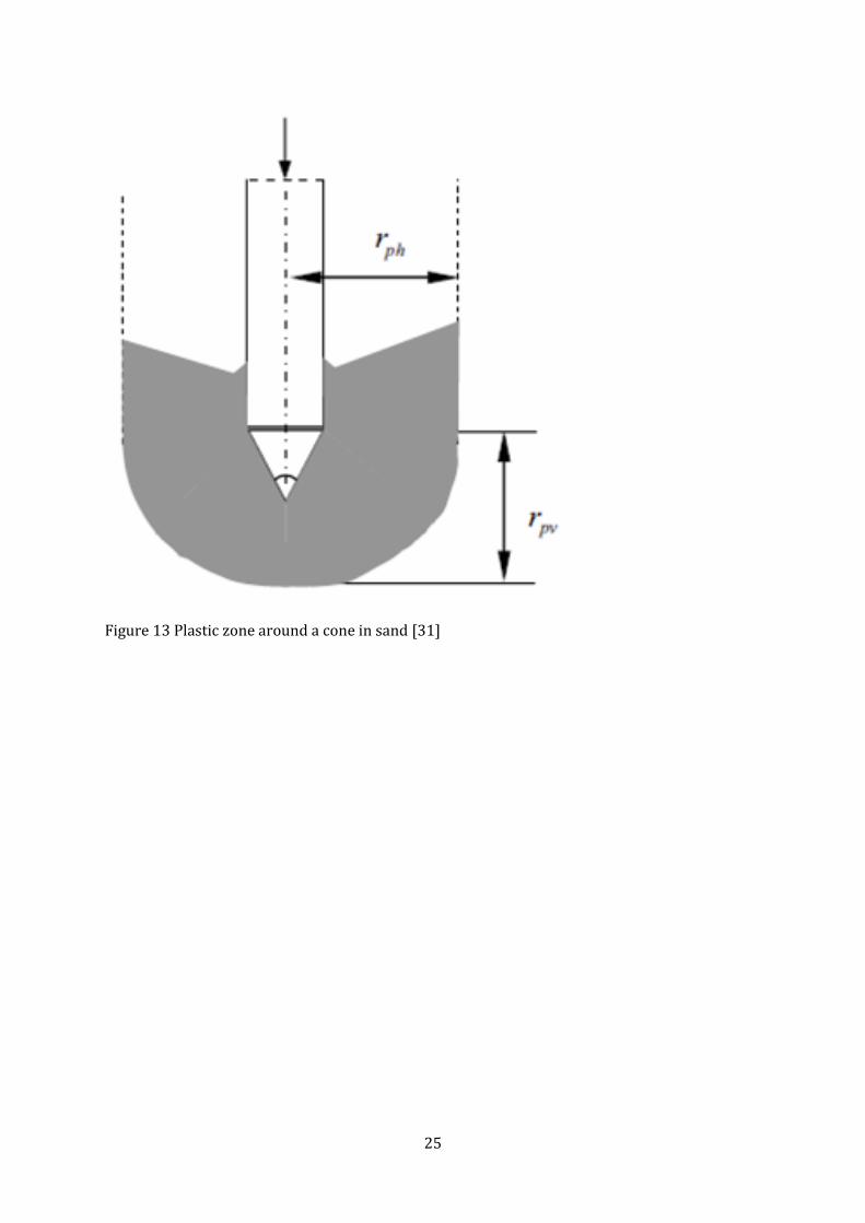
This method was encouraged by a recent finite element study of cone penetration in sand [31].

They proposed that the plastic zone created behind the cone and around the shaft of a

penetrometer is similar to that predicted by applying cylindrical cavity expansion theory.

However, the shape of the elastic-plastic boundary around the cone tip and face is assumed to

be circular or elliptical as shown in Figure 13. By applying the above assumption and using the

cavity expansion solutions in Mohr-Coulomb materials, as derived by Yu [13] and Yu and Carter

[14], cone tip resistance, qc, in a purely frictional soil can be obtained using the following

expression:

𝑞c

𝑃0′=

3𝛼

2 + 𝛼(𝐹

𝑐

𝑎)

2(𝛼−1)𝛼

(3)

where P0’ is the initial mean effective stress, F is the plastic zone shape factor and taken to be

unity for a circular plastic zone around the cone (i.e., rph = rpv in Figure 13), or otherwise less

than 1.0. From numerical studies, Yu [13, 30] assumed F to be between 0.7–0.8. The ratio (c / a)

is the relative size of the plastic zone generated as a result of expanding a cylindrical cavity from

zero radius. Yu [13] derived an analytical solution to this by solving the simple non-linear

equation for a purely frictional soil:

1 = 𝛾 (

𝑐

𝑎)

𝛼−1𝛼

+ [2𝛿 − 𝛾] (𝑐

𝑎)

𝛽+1𝛽

(4)

where γ, δ, α, β, s and x are constant, derived parameters, and are defined in equations (5) to

(10) as follows:

𝛾 =

𝛼𝛽𝑠

𝛼 + 𝛽 (5)

9

𝛿 =

(α − 1)𝑃0

2(1 + α)𝐺 (6)

𝛼 = 1 + sin 𝜙

1 − sin 𝜙 (7)

𝛽 = 1 + sin 𝜓

1 − sin 𝜓 (8)

𝑠 = 𝑥(1 − 𝛼)

𝛼𝛽 (9)

𝑥 = (1 − 𝜈)𝛼𝑃0′

((𝛼)2 − 1)𝐺 {[𝛽 −

𝜈

1 − 𝜈] +

1

𝛼[1 −

𝜈𝛽

1 − 𝜈]} (10)

and where G is the shear modulus.

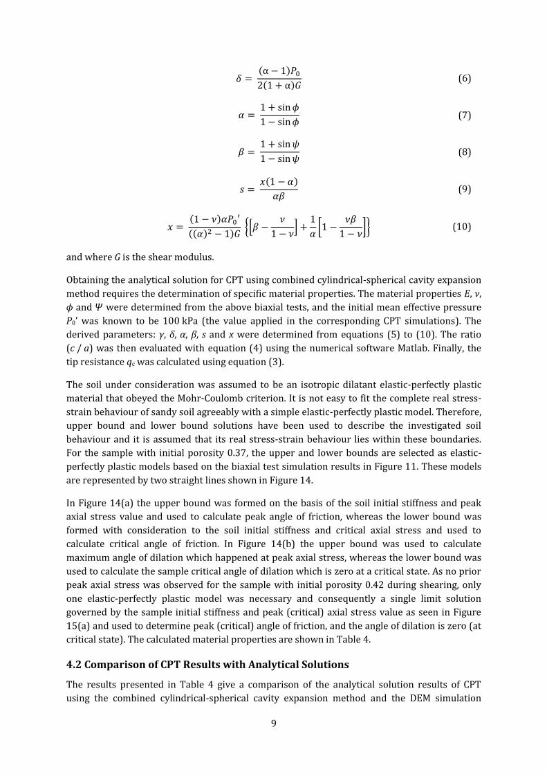
Obtaining the analytical solution for CPT using combined cylindrical-spherical cavity expansion

method requires the determination of specific material properties. The material properties E, ν,

ϕ and 𝛹 were determined from the above biaxial tests, and the initial mean effective pressure

P0’ was known to be 100 kPa (the value applied in the corresponding CPT simulations). The

derived parameters: γ, δ, α, β, s and x were determined from equations (5) to (10). The ratio

(c / a) was then evaluated with equation (4) using the numerical software Matlab. Finally, the

tip resistance qc was calculated using equation (3).

The soil under consideration was assumed to be an isotropic dilatant elastic-perfectly plastic

material that obeyed the Mohr-Coulomb criterion. It is not easy to fit the complete real stress-

strain behaviour of sandy soil agreeably with a simple elastic-perfectly plastic model. Therefore,

upper bound and lower bound solutions have been used to describe the investigated soil

behaviour and it is assumed that its real stress-strain behaviour lies within these boundaries.

For the sample with initial porosity 0.37, the upper and lower bounds are selected as elastic-

perfectly plastic models based on the biaxial test simulation results in Figure 11. These models

are represented by two straight lines shown in Figure 14.

In Figure 14(a) the upper bound was formed on the basis of the soil initial stiffness and peak

axial stress value and used to calculate peak angle of friction, whereas the lower bound was

formed with consideration to the soil initial stiffness and critical axial stress and used to

calculate critical angle of friction. In Figure 14(b) the upper bound was used to calculate

maximum angle of dilation which happened at peak axial stress, whereas the lower bound was

used to calculate the sample critical angle of dilation which is zero at a critical state. As no prior

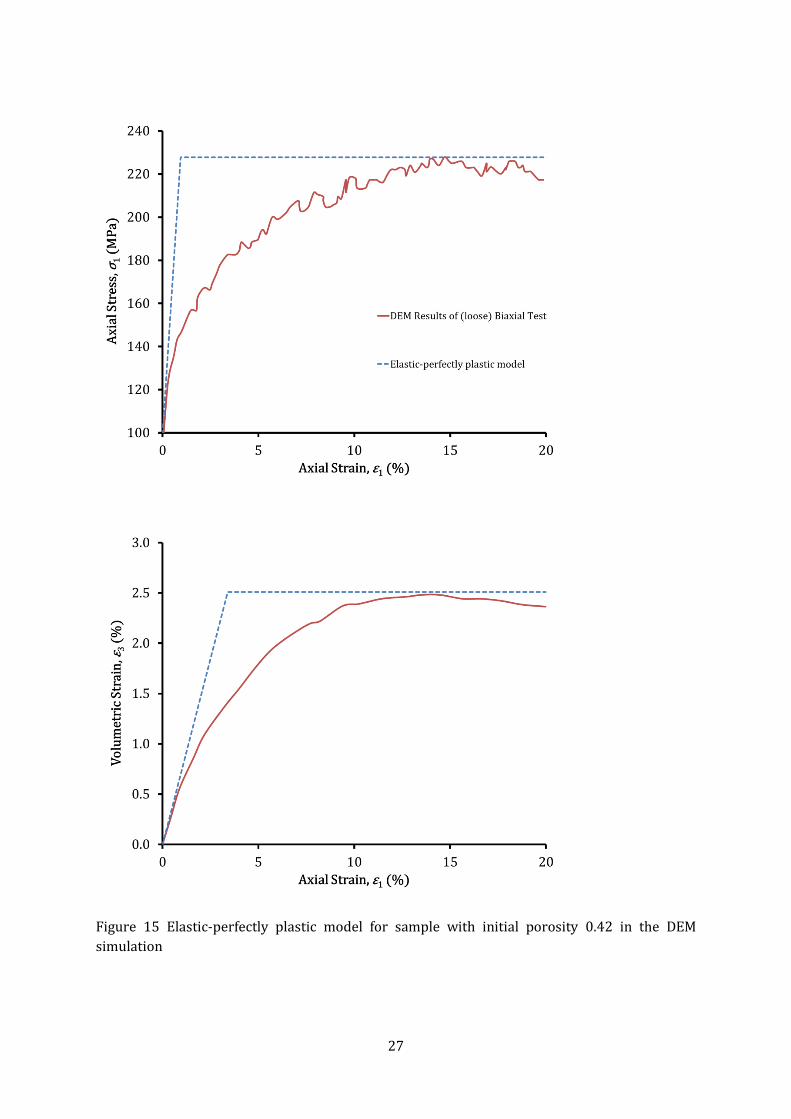
peak axial stress was observed for the sample with initial porosity 0.42 during shearing, only

one elastic-perfectly plastic model was necessary and consequently a single limit solution

governed by the sample initial stiffness and peak (critical) axial stress value as seen in Figure

15(a) and used to determine peak (critical) angle of friction, and the angle of dilation is zero (at

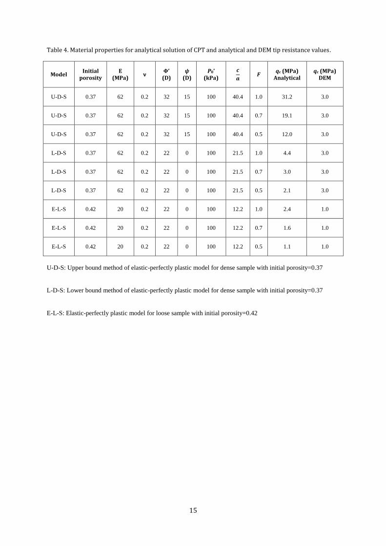
critical state). The calculated material properties are shown in Table 4.

4.2 Comparison of CPT Results with Analytical Solutions

The results presented in Table 4 give a comparison of the analytical solution results of CPT

using the combined cylindrical-spherical cavity expansion method and the DEM simulation

10

results for a sample of spheres. It can be seen that for the sample with initial porosity of 0.37

(the dense sample obtained from the DEM simulation), the upper bound solution led to an

analytical tip resistance value of 31.2 MPa for a plastic zone shape factor F = 1. However, this

value decreased to 19.1 MPa for F=0.7 and to 12.0 MPa for F = 0.5. On the other hand, when the

lower bound solution was considered for the same sample, it resulted in an analytical tip

resistance value of 4.4 MPa for a plastic zone factor F = 1; this value decreased to 3.0 MPa for

F = 0.7 and to 2.1 MPa for F = 0.5. As expected, the 3 MPa tip resistance as obtained from the

DEM simulation for the sample with initial porosity 0.37 lies between the upper bound and

lower bound values of the analytical solutions for F = 0.5. For the sample with an initial porosity

of 0.42 (the loose sample obtained from DEM simulation), only one elastic-perfectly plastic

model used to describe the soil behaviour, resulted in an analytical tip resistance value of

2.4 MPa for a plastic zone factor F = 1. However, this value decreased to 1.6 MPa for F = 0.7 and

to 1.1 MPa for F = 0.5. In this regard, the tip resistance value of 1 MPa obtained from the DEM

simulation for the sample with initial porosity of 0.42 is consistent with the analytical solution

for F = 0.5 to within about 10%.

The results suggest that DEM can be used to simulate cone penetration tests in granular

materials, and have shown reasonable agreement with theoretical analytical solutions. This

analysis highlights the important effect of the plastic zone shape factor on the magnitude of tip

resistance, and a value for F of 0.5 gives an appropriate analytical tip resistance value compared

with the numerical one.

In reality the plastic zone shape factor F would vary to some extent with soil types and their

mechanical properties, as it is defined to reflect the shape of the plastic zone around the cone

tip. A value of F = 1 means that the plastic zone is circular. The range of F = 0.7–0.8 that was

suggested by Yu [30] was based on limited large strain finite element analyses of cone

penetration in sand carried out by Huang et al [31]. Clearly more work, both numerical and

experimental, is needed in order to determine the true range of F for various real soils.

5 Conclusions A numerical analysis of cone penetration tests in a granular material in a calibration chamber

has been investigated using DEM. A particle refinement was implemented in the simulations

whereby small particles were generated near the cone penetrometer and larger particles

further away to achieve a higher number of small particles in contact with the cone tip. Using a

radius expansion method during sample preparation was found to reduce computational time

significantly compared with the deposition and compaction method without affecting tip

resistance too much. In addition, because the CPT test is a quasi-static process, it was found that

the use of a constant particle mass, irrespective of size, lead to a larger time-step and greater

computational efficiency compared with constant density and almost the same tip resistance

was obtained in both cases. The paper has not attempted to model a specific penetration

resistance profile as a function of depth, but does replicate qualitatively the correct behaviour

and the effect of different parameters such as initial porosity, mean effective stress and particle

friction coefficient have been shown to have an effect on the behaviour. A reduction in particle

size next to the cone was found to give a higher tip resistance especially at shallow depths and

decrease the fluctuations in the tip resistance. The initial porosity, mean effective stress and

particle friction coefficient were found to influence the tip resistance, with a reduction in initial

11

porosity, an increase in particle friction coefficient and an increase in mean effective stress all

leading to an increase in tip resistance.

DEM simulations of biaxial tests were carried out and suitable continuum parameters were

obtained for input to an analytical cavity expansion solution for cone tip resistance based on

continuum mechanics and a combined cylindrical-spherical cavity expansion method. A

comparison is provided between the DEM-derived cone tip resistance and a simple cavity

expansion–based analytical solution, with an estimated F-value. The study shows it has been

possible to capture the essential features of the mechanics of cone penetration in granular

materials using DEM, therefore showing that DEM can be used to simulate cone penetration

tests in granular materials with confidence. Hence this new combined DEM-cavity expansion

approach adds new insight to the complex cone penetration problem in geotechnical

engineering.

The next step will be to improve the realism of CPT simulations, which the authors believe will

be a more feasible task now it has been established how the efficiency of the model can be

improved. This future work will involve combining the key concepts of the above work with

realistic shape [17], a vastly greater number of particles, polydisperse particle assemblies, a Hertzian

contact law, and realistic, calibrated micro properties for both the particles and apparatus.

References 1. Mayne, P.W.: In-Situ Test Calibrations for Evaluating Soil Parameters. In: Phoon, K.. K..,

Hight, D.. W.., Leroueil, S.., and Tan, T.. S.. (eds.) Characterization and engineering properties of natural soils. pp. 1–56. Taylor and Francis (2006).

2. Parkin, A.K., Lunne, T.: Boundary Effects in the Laboratory Calibration of a Cone Penetrometer for Sand. Nor. Geotech. Inst. Publ. (1982).

3. Salgado, R., Mitchell, J.K., Jamiolkowski, M.: Calibration Chamber Size Effects on Penetration Resistance in Sand. J. Geotech. Geoenvironmental Eng. 124, 878–888 (1998).

4. Huang, A., Hsu, H.: Advanced calibration chambers for cone penetration testing in cohesionless soils. In: Viana, A. and Mayne, P.W. (eds.) ISC-2 Geotechnical and Geophysical Site Characterization. pp. 147–166. Millpress Science Publishers, National Chiao Tung University (2004).

5. Susila, E., Hryciw, R.D.: Large displacement FEM modelling of the cone penetration test (CPT) in normally consolidated sand. Int. J. Numer. Anal. Methods Geomech. 27, 585–602 (2003).

6. Ahmadi, M.M., Byrne, P.M., Campanella, R.G.: Cone tip resistance in sand: modeling, verification, and applications. Can. Geotech. J. 42, 977–993 (2005).

7. Huang, A.-B., Ma, M.Y.: An analytical study of cone penetration tests in granular material. Can. Geotech. J. 31, 91–103 (1994).

8. Calvetti, F., Nova, R.: Micro-macro relationships from DEM simulated element and in-situ tests. Powders and Grains-Garcia-Rojo, Herrmann and McNamara(eds). pp. 245–249 (2005).

9. Jiang, M.J., Yu, H.S., Harris, D.: Discrete element modelling of deep penetration in granular soils. Int. J. Numer. Anal. methods Geomech. 30, 335–361 (2006).

10. ARROYO, M., BUTLANSKA, J., CALVETTI, F., GENS, A., JAMIOLKOWSKI, M.: Cone penetration tests in a virtual calibration chamber. Géotechnique. 61, 525–531 (2010).

11. Jamiolkowski, M., Lo Presti, D.C.F., Manassero, M.: Evaluation of relative density and shear strength of sands from CPT and DMT. Geotechnical Special Publication. pp. 201–238 (2003).

12. McDowell, G.R., Falagush, O., Yu, H.-S.: A particle refinement method for simulating DEM of cone penetration testing in granular materials. Géotechnique Lett. 2, 141–147 (2012).

12

13. Yu, H.: Cavity expansion methods in geomechanics. Kluwer Academic Publishers, NL (2000).

14. Yu, H.S., Carter, J.P.: Rigorous Similarity Solutions for Cavity Expansion in Cohesive‐Frictional Soils. (2002).

15. Falagush, O., McDowell, G., Yu, H.: Discrete element modelling of cone penetration tests in granular materials. In: Coutinho and Mayne (eds.) Geotechnical and Geophysical Site Characterization 4. pp. 257–262. Taylor & Francis (2012).

16. Schnaid, F.: A study of the cone-pressuremeter test in sand, PhD Thesis, University of Oxford, (1990).

17. Falagush, O., Mcdowell, G.R., Yu, H.: Discrete Element Modeling of Cone Penetration Tests Incorporating Particle Shape and Crushing. Int. J. Geomech. published online (2015).

18. Itasca: Particle Flow Code in 3 Dimensions. Itasca Consulting Group, Inc., Minneapolis, Minnesota (2005).

19. Falagush, O.: Discrete element modelling of cone penetration testing in granular materials, PhD Thesis, University of Nottingham, http://eprints.nottingham.ac.uk/14134/1/Omar_Falagush-_thesis.pdf, (2014).

20. De Beer, E.E., Goelen, E., Heynen, W.J., Joustra, K.: Cone penetration test (CPT): international reference test procedure. Int. J. Rock Mech. Min. Sci. Geomech. Abstr. 27, A93 (1990).

21. Schmertmann, J.: An updated correlation between relative density, Dr, and Fugro-type electric cone bearing, qc. Contract Rep. DACW. (1976).

22. Villet, W.C.B., Mitchell, J.K.: Cone Resistance, Relative Density and Friction Angle. Cone Penetration Testing and Experience. pp. 178–208. ASCE (1981).

23. Baldi, G., Bellotti, R., Ghionna, V.: Design parameters for sands from CPT. Proc. Second Eur. Symp. Penetration Test. 11, 425–432 (1982).

24. Baldi, G., Bellotti, R., Ghionna, V.: Interpretation of CPTs and CPTUs; 2nd part: drained penetration of sands. Proceedings of the Fourth International Geotechnical Seminar. pp. 143–156. , Singapore (1986).

25. Lee, K.L., Seed, H.B.: Drained Strength Characteristics of Sands. J. Soil Mech. Found. Div. Am. Soc. Civ. Eng. 93, 117–141 (1967).

26. Schanz, T., Vermeer, P.: Angles of friction and dilatancy of sand. Géotechnique. 46, 145–152 (1996).

27. Ni, Q.: Effects of particle properties and boundary conditions on soil shear behaviour: 3-D numerical simulations, PhD Thesis, University of Southampton, (2003).

28. Bishop, R.F., Hill, R., Mott, N.F.: The theory of indentation and hardness tests. Proc. Phys. Soc. 57, 147–159 (1945).

29. Yu, H.S., Mitchell, J.K.: Analysis of Cone Resistance: Review of Methods. J. Geotech. Geoenvironmental Eng. 124, 140–149 (1998).

30. Yu, H.S.: The First James K. Mitchell Lecture In situ soil testing: from mechanics to interpretation. Geomech. Geoengin. 1, 165–195 (2006).

31. Huang, W., Sheng, D., Sloan, S.W., Yu, H.S.: Finite element analysis of cone penetration in cohesionless soil. Comput. Geotech. 31, 517–528 (2004).

13

Tables

Table 1. Dimensions and boundary conditions of experimental and numerical calibration chamber.

Setting Units Experimental

calibration chamber

Numerical calibration

chamber

Chamber width (D) (mm) 1000 300

Chamber height (H) (mm) 1500 100

Cone diameter (B) (mm) 36 18

Particles size (𝑑50) (mm) 0.8 1.0

Vertical and horizontal stresses (kPa) 100 100

(𝐷𝑐 𝐵⁄ ) ratio - 27.78 16.67

(𝐵 𝑑50⁄ ) ratio - 45 18

Table 2. Particle and wall properties for DEM simulations.

Input parameter Value

Particle and wall normal stiffness (𝑘𝑛) 5x105N/m

Particle and wall shear stiffness (𝑘𝑠) 5x105N/m

Particle density 2650kg/m3

Particle coefficient of friction 0.5

Frictional tip cone coefficient of friction 0.5

Frictional sleeve coefficient of friction 0.5

Chamber wall coefficient of friction 0

14

Table 3. Summary of CPT simulations.

Simulation

Sample

preparation

method

Particle

mass

Model

angle

(degrees)

No. of

zones

Zone

external

radius

(mm)

Zone

particle

size

(mm)

Number

of

particles

Initial

porosity

Isotropic

stresses

(kPa)

Average

model

run

(days)

A Compactio

n method

Variable

mass 30 3 75,95,150 2,3,4 33600 0.37 300 30

B

Radius

expansion

method

Variable mass

30 3 75,95,150 2,3,4 34700 0.37 300 7

C

Radius

expansion

method

Constant

mass 30 3 75,95,150 2,3,4 34700 0.37 300 3

D

Radius

expansion

method

Constant mass

30 5 20,35,50,65,1

50 1,1.5,2,3,

4 37050 0.37 300 5

E Radius

expansion

method

Constant

mass 30 5

20,35,50,65,1

50

1,1.5,2,3,

4 37050 0.37 100 5

F Radius

expansion

method

Constant

mass 30 5

20,35,50,65,1

50

1,1.5,2,3,

4 37050 0.42 100 5

G

Radius

expansion method

Constant

mass 30 5

20,35,50,65,1

50

1,1.5,2,3,

4 37050 0.37 200 5

H

Radius

expansion method

Constant

mass 30 5

20,35,50,65,1

50

1,1.5,2,3,

4 37050 0.37 100 5

I

Radius

expansion

method

Constant mass

30 5 20,35,50,65,1

50 1,1.5,2,3,

4 37050 0.37 100 5

15

Table 4. Material properties for analytical solution of CPT and analytical and DEM tip resistance values.

Model Initial

porosity E

(MPa) ν

Φ’ (D)

ψ (D)

P0’ (kPa)

𝒄

𝒂 𝑭

qc (MPa) Analytical

qc (MPa) DEM

U-D-S 0.37 62 0.2 32 15 100 40.4 1.0 31.2 3.0

U-D-S 0.37 62 0.2 32 15 100 40.4 0.7 19.1 3.0

U-D-S 0.37 62 0.2 32 15 100 40.4 0.5 12.0 3.0

L-D-S 0.37 62 0.2 22 0 100 21.5 1.0 4.4 3.0

L-D-S 0.37 62 0.2 22 0 100 21.5 0.7 3.0 3.0

L-D-S 0.37 62 0.2 22 0 100 21.5 0.5 2.1 3.0

E-L-S 0.42 20 0.2 22 0 100 12.2 1.0 2.4 1.0

E-L-S 0.42 20 0.2 22 0 100 12.2 0.7 1.6 1.0

E-L-S 0.42 20 0.2 22 0 100 12.2 0.5 1.1 1.0

U-D-S: Upper bound method of elastic-perfectly plastic model for dense sample with initial porosity=0.37

L-D-S: Lower bound method of elastic-perfectly plastic model for dense sample with initial porosity=0.37

E-L-S: Elastic-perfectly plastic model for loose sample with initial porosity=0.42

16

Figures

Figure 1 Sample of three particle sizes in a 30° segment of calibration chamber

17

Figure 2 Boundary conditions for cone penetrometer

18

Figure 3 Tip resistance results for simulations A and B

Figure 4 Tip resistance results for simulations B and C

19

Figure 5 Tip resistance results for simulations C and D

Figure 6 Influence of the whole sample initial porosity on tip resistance

20

Figure 7 Influence of mean effective stress on tip resistance, qc (for the dense sample)

Figure 8 Influence of mean effective stress on normalised tip resistance, Q = qc / σh

21

Figure 9 Influence of particle friction coefficient on tip resistance at 100 kPa compressive stress

(for the dense sample)

22

Figure 10 Sample for biaxial test simulation

23

Figure 11 Axial stress and volumetric dilation for samples with two different initial porosities:

(a) Axial stress against axial strain (b) Volumetric strain against axial strain

24

Figure 12 Estimating of elastic properties (a) Young’s modulus (b) Poisson’s ratio

25

Figure 13 Plastic zone around a cone in sand [31]

26

Figure 14 Upper and lower bounds for sample with initial porosity 0.37 in the DEM simulation

27

Figure 15 Elastic-perfectly plastic model for sample with initial porosity 0.42 in the DEM

simulation