facts devices chapter 1 2 3 4

FACTS Devices 1

FACTS (Flexible Alternating Current Transmission Systems) Devices

Course objectives: study / learning / knowledge:

- transit (transfer/transmission) power through electrical transmission lines;

- different compensation techniques for power transmission lines;

- FACTS devices;

- design of FACTS devices;

- advantages and disadvantages of introducing FACTS devices.

References

1. Adam M., Baraboi A., Electronică de putere, Editura VENUS, Iaşi, 2005.

2. Baraboi A., Ciutea I., Adam M., Hnatiuc E., Tehnici moderne în comutaţia de putere.

Editura A 92, Iaşi, 1996.

3. Eremia M., Tehnici noi în transportul energiei electrice. Aplicaţii ale electronicii de putere.

Editura Tehnică, Bucureşti, 1997.

4. Hingorani N. G., Gyugyi L., Understanding FACTS. Concepts and Technology of Flexible

AC Transmission Systems. IEEE Press, New York, 2000.

5. Ionescu F., Six J. P., Floricău D., Delarue Ph., Niţu Smaranda, Boguş C., Electronică de

putere. Editura Tehnică, Bucureşti, 1998.

6. Rashid M. H., Power Electronics Circuits, Devices, and Applications, Pearson Prentice

Hall, USA, 2004.

7. Séguier G., Bausière R., Labrique F., Électronique de puissance. Dunod, Paris, 2004.

FACTS Devices 2

1. Generalities

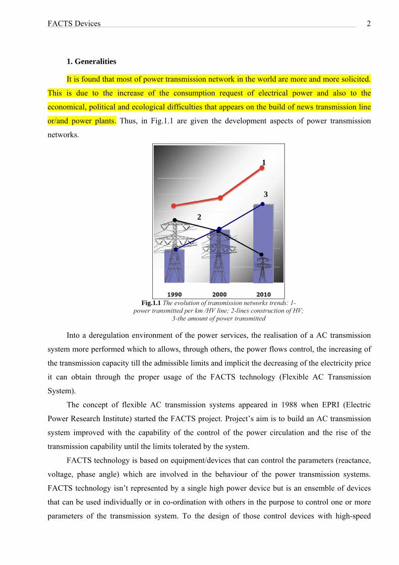
It is found that most of power transmission network in the world are more and more solicited.

This is due to the increase of the consumption request of electrical power and also to the

economical, political and ecological difficulties that appears on the build of news transmission line

or/and power plants. Thus, in Fig.1.1 are given the development aspects of power transmission

networks.

Fig.1.1 The evolution of transmission networks trends: 1-

power transmitted per km /HV line; 2-lines construction of HV; 3-the amount of power transmitted

1

3

2

Into a deregulation environment of the power services, the realisation of a AC transmission

system more performed which to allows, through others, the power flows control, the increasing of

the transmission capacity till the admissible limits and implicit the decreasing of the electricity price

it can obtain through the proper usage of the FACTS technology (Flexible AC Transmission

System).

The concept of flexible AC transmission systems appeared in 1988 when EPRI (Electric

Power Research Institute) started the FACTS project. Project’s aim is to build an AC transmission

system improved with the capability of the control of the power circulation and the rise of the

transmission capability until the limits tolerated by the system.

FACTS technology is based on equipment/devices that can control the parameters (reactance,

voltage, phase angle) which are involved in the behaviour of the power transmission systems.

FACTS technology isn’t represented by a single high power device but is an ensemble of devices

that can be used individually or in co-ordination with others in the purpose to control one or more

parameters of the transmission system. To the design of those control devices with high-speed

FACTS Devices 3

feedback is possible because of the progresses reached in the filed of power electronics,

microelectronics and microprocessors.

Flexible transmission systems based on power electronic equipment with high speed response

provides the following possibilities for increasing efficiency in the AC transmission:

- power control and thus the possibility to prescribe the power circulations (transits) on

electrical lines of looped network (to avoid power flows in loop);

- safe loading of transmission lines at levels close to thermal limits;

- the exit prevention of operation, in cascade of the installations by limiting the effects of

incidents;

- increasing the transmission capacity in the controlled systems so that the power reserve,

which is typically 18% may be reduced to 15% or less;

- attenuation of oscillations in power systems which can damage the equipment and limit

transmission capacity.

Into a loop power network the distribution of real power between the various power plants

and the circulations to consumption centers are made by physical laws and not always economic.

The reactive power influences, at its turn, the distribution of real power by changing the voltage

levels, because the transmission lines are producing or consuming of reactive power in according

with their degree of charge.

For the control the real and reactive power flows into the AC network there are, at present, the

following possibilities:

- phase shifter transformer (rotating);

- series compensator with coils and capacitors;

- controllers for the output voltage of generators;

- shunt compensator (transverse).

The performances obtained in high power converters for DC transmission have led to the

realization of devices capable to control the real and/or reactive power flows into the AC networks.

These devices grouped under the concept FACTS, include: static shunt compensator

(transverse) with electronic switching, thyristor controlled series compensator, phase shifter

transformer with electronic control in load, sub-synchronous oscillations damper. There are

concerns, currently, for realization these devices with static converters in forced switching,

achieving so-called "advanced FACTS devices".

The IEEE Working Group with 14 Study Committee of CIGRE proposed the following

definition of the concept FACTS, this represents:

FACTS Devices 4

“The Flexible AC Transmission System (FACTS) is a new technology based on power

electronic devices which offers an opportunity to enhance controllability, stability and power

transfer capability of AC Transmission Systems”.

2. Power flows control necessity The control necessity of power flows in transmission lines of power systems is supported by

the following examples.

2.1. Power flow in parallel electrical lines

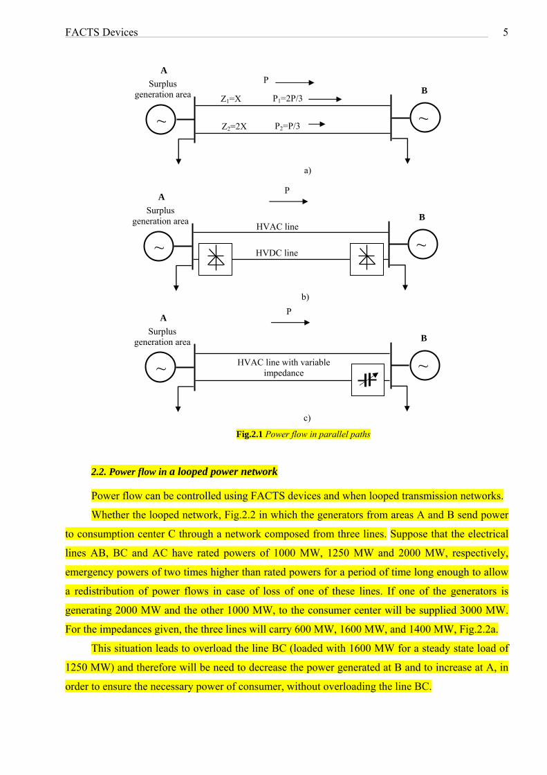
We consider a simple case of power transit by two parallel paths from a surplus generation

area, represented as an equivalent source on the left and a deficit generation area on the right,

Fig.2.2a. In the absence of any control, the repartition of power flows is based on the inverse of the

transmission line impedances. Apart from ownership and contractual issues regarding how much

power support the lines, it is possible that the lower impedance line may become overloaded and

thereby limits the loading on both paths even if higher impedance path is not fully loaded.

Figure 2.2b shows the same two paths, but one of these has HVDC transmission. In this case

power flow is determined by the operator, because using power electronic converters, the power

flow is electronically controlled. Also, because the power flow is electronically controlled, the

HVDC line can be used to its full thermal capacity if there are adequate capacity converters. More

than that, a HVDC line, due to the very high response speed can also help that the parallel AC

transmission line to maintain stability. However, the HVDC line is expensive and can be considered

only if transmission distances are long.

Another way to control the power flow is using FACTS devices. Using the impedance

control, Fig.2.2c, or phase angle, or by injecting an appropriate voltage, a FACTS device can

control the power flow as it is desired.

FACTS Devices 5

AP

Fig.2.1 Power flow in parallel paths 2.2. Power flow in a looped power network

Power flow can be controlled using FACTS devices and when looped transmission networks.

Whether the looped network, Fig.2.2 in which the generators from areas A and B send power

to consumption center C through a network composed from three lines. Suppose that the electrical

lines AB, BC and AC have rated powers of 1000 MW, 1250 MW and 2000 MW, respectively,

emergency powers of two times higher than rated powers for a period of time long enough to allow

a redistribution of power flows in case of loss of one of these lines. If one of the generators is

generating 2000 MW and the other 1000 MW, to the consumer center will be supplied 3000 MW.

For the impedances given, the three lines will carry 600 MW, 1600 MW, and 1400 MW, Fig.2.2a.

This situation leads to overload the line BC (loaded with 1600 MW for a steady state load of

1250 MW) and therefore will be need to decrease the power generated at B and to increase at A, in

order to ensure the necessary power of consumer, without overloading the line BC.

Surplus generation area B

P1=2P/3Z1=X

~~ P2=P/3 Z2=2X

a)

P A


HVAC line

~~ HVDC line

b)

P A


~~ HVAC line with variable impedance

c)

FACTS Devices 6

Fig.2.2 Power flow in a looped network: a) looped network diagram; b) looped network equipped with series capacitor on the line AC; c) looped network equipped with reactor on line BC

3000 MW

~A

P1=1400MW

10 C

B1000 MW

2000 MW

a)

~

10 5 P2=600 MW

P3=1600MW

P1=1750MW

~C

A 10

B1000 MW

2000 MW

b)

~

10 5 P2=250 MW

P3=1250MW

-5

3000 MW

~A 10

B

P1=1750MW 2000 MW C

1000 MW

c)

3000 MW5 10 P2=250 MW

P3=1250MW7

~

FACTS Devices 7

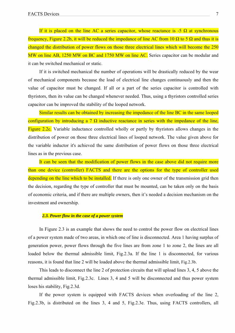
If it is placed on the line AC a series capacitor, whose reactance is -5 Ω at synchronous

frequency, Figure 2.2b, it will be reduced the impedance of line AC from 10 Ω to 5 Ω and thus it is

changed the distribution of power flows on those three electrical lines which will become the 250

MW on line AB, 1250 MW on BC and 1750 MW on line AC. Series capacitor can be modular and

it can be switched mechanical or static.

If it is switched mechanical the number of operations will be drastically reduced by the wear

of mechanical components because the load of electrical line changes continuously and then the

value of capacitor must be changed. If all or a part of the series capacitor is controlled with

thyristors, then its value can be changed whenever needed. Thus, using a thyristors controlled series

capacitor can be improved the stability of the looped network.

Similar results can be obtained by increasing the impedance of the line BC in the same looped

configuration by introducing a 7 Ω inductive reactance in series with the impedance of the line,

Figure 2.2c. Variable inductance controlled wholly or partly by thyristors allows changes in the

distribution of power on those three electrical lines of looped network. The value given above for

the variable inductor it's achieved the same distribution of power flows on those three electrical

lines as in the previous case.

It can be seen that the modification of power flows in the case above did not require more

than one device (controller) FACTS and there are the options for the type of controller used

depending on the line which to be installed. If there is only one owner of the transmission grid then

the decision, regarding the type of controller that must be mounted, can be taken only on the basis

of economic criteria, and if there are multiple owners, then it’s needed a decision mechanism on the

investment and ownership.

2.3. Power flow in the case of a power system

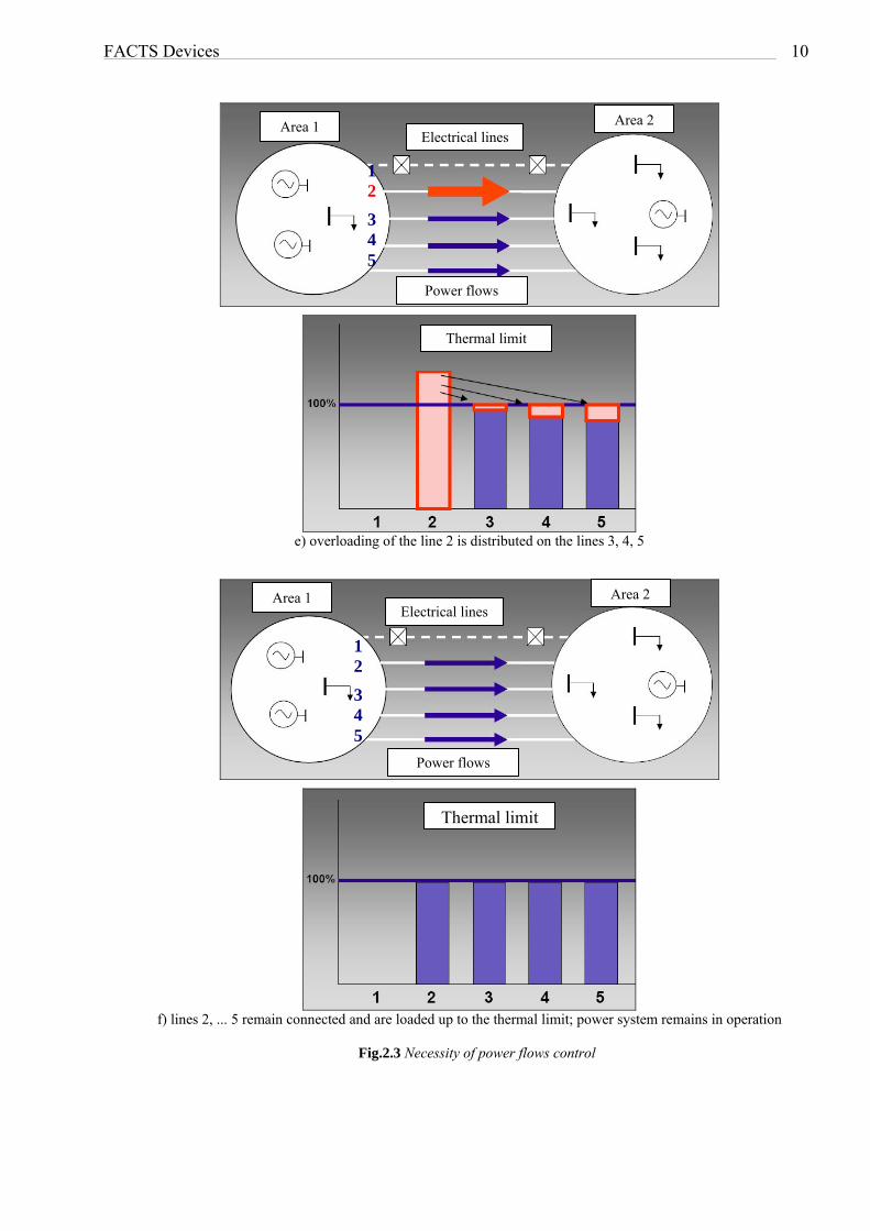
In Figure 2.3 is an example that shows the need to control the power flow on electrical lines

of a power system made of two areas, in which one of line is disconnected. Area 1 having surplus of

generation power, power flows through the five lines are from zone 1 to zone 2, the lines are all

loaded below the thermal admissible limit, Fig.2.3a. If the line 1 is disconnected, for various

reasons, it is found that line 2 will be loaded above the thermal admissible limit, Fig.2.3b.

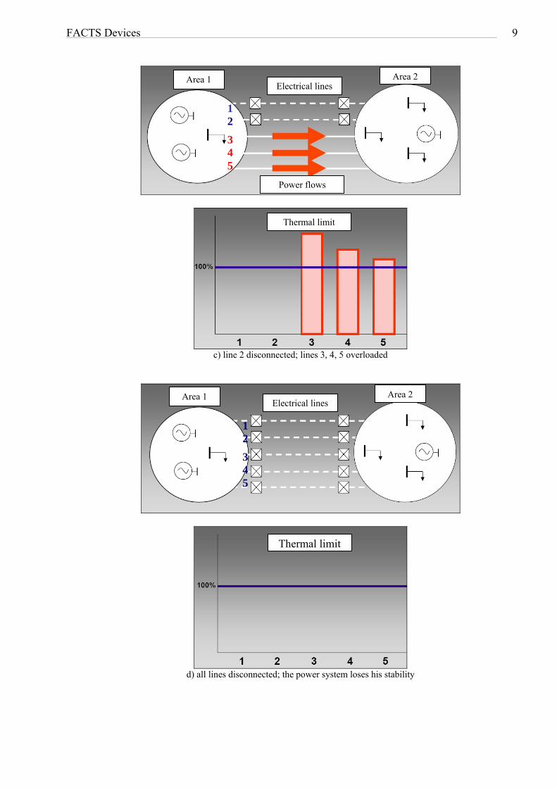
This leads to disconnect the line 2 of protection circuits that will upload lines 3, 4, 5 above the

thermal admissible limit, Fig.2.3c. Lines 3, 4 and 5 will be disconnected and thus power system

loses his stability, Fig.2.3d.

If the power system is equipped with FACTS devices when overloading of the line 2,

Fig.2.3b, is distributed on the lines 3, 4 and 5, Fig.2.3e. Thus, using FACTS controllers, all

FACTS Devices 8

connected lines will be loaded up to the thermal admissible limit and power system remains in

operation, Fig.2.3f.

Area 2 Area 1 Electrical lines

1 2 3 4 5

Power flows

Thermal limit

a) lines loaded under the thermal limit


1 2

3 4 5

Power flows

Thermal limit

b) line 1 disconnected; line 2 overloaded

FACTS Devices 9


1 2

3 4 5

Power flows

Thermal limit

c) line 2 disconnected; lines 3, 4, 5 overloaded


1 2

3 4 5

Thermal limit

d) all lines disconnected; the power system loses his stability

FACTS Devices 10


1 2

3 4 5

Power flows

Thermal limit

e) overloading of the line 2 is distributed on the lines 3, 4, 5


1 2

3 4 5

Power flows

Thermal limit

f) lines 2, ... 5 remain connected and are loaded up to the thermal limit; power system remains in operation

Fig.2.3 Necessity of power flows control

FACTS Devices 11

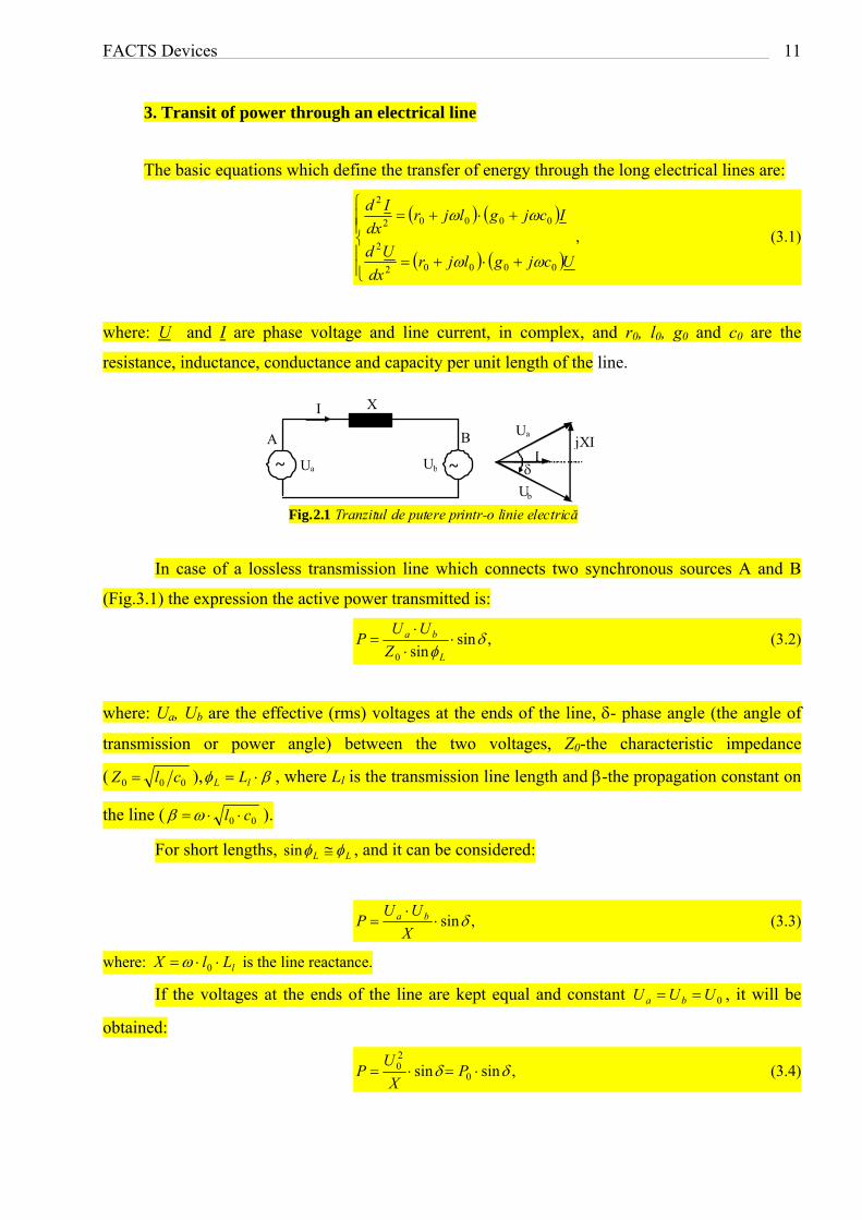
3. Transit of power through an electrical line

The basic equations which define the transfer of energy through the long electrical lines are:

,

00002

2

00002

2

Ucjgljrdx

Ud

Icjgljrdx

Id

(3.1)

where: U and I are phase voltage and line current, in complex, and r0, l0, g0 and c0 are the

resistance, inductance, conductance and capacity per unit length of the line.

jXII

Ua

Ub

~ ~Ua Ub

X

A B

I

Fig.2.1 Tranzitul de putere printr-o linie electrică

In case of a lossless transmission line which connects two synchronous sources A and B

(Fig.3.1) the expression the active power transmitted is:

,sinsin0

L

ba

Z

UUP (3.2)

where: Ua, Ub are the effective (rms) voltages at the ends of the line, - phase angle (the angle of

transmission or power angle) between the two voltages, Z0-the characteristic impedance

( 000 clZ ), lL L , where Ll is the transmission line length and -the propagation constant on

the line ( 00 cl ).

For short lengths, LL sin , and it can be considered:

,sin

X

UUP ba (3.3)

where: lLlX 0 is the line reactance.

If the voltages at the ends of the line are kept equal and constant U , it will be 0UUba

obtained:

,sinsin 0

20 P

X

UP (3.4)

FACTS Devices 12

where P0 is the natural power (around 500 MW for a line of 400 kV with a characteristic impedance

Z0= 300 ).

Reactive power exchanged between the sources and line, under the same conditions, is:

.)cos1(20

X

UQ (3.5)

The theoretical possibilities for adjusting the power flow, according to equation (3.3) are:

- changing of the RMS voltages Ua and Ub (in reality they can be modified only in reduced

limits);

- changing of the reactance X of the transmission line;

- changing the transmission angle, .

In Fig.3.2 is shown the variation of active and reactive power depending on the transmission

angle , it is observing that the active power is maximum for =900.

The stable part of the characteristic P() corresponds to the values = 00... 900, in practice

it’s operating, for reasons of stability of the generators, with a coefficient of static stability KS

between 1.15 ... 1.20 and an angle between 350... 400.

The coefficient KS is defined by the relation:

,0

P

PSK (3.6)

where: P0 is the maximum power, and P – the power produced by the generator.

The operating points from the characteristic P () which satisfy the condition:

,0P

(3.7)

ratio called static stability criterion, are stable operating points.

Fig.3.2 Evolution of active and reactive power depending on the transmission angle

[°]

0

P0

2P0

0 30 60 90 120 150 180

P Q

P

Q

FACTS Devices 13

4. The dynamic stability of the generators

It considers a generator that supply a busbar of infinite power system through two parallel

lines, characterized by the inductive reactances X1. In the diagram from Fig.4.1 there are shown

three characteristics of the power generator, as follows: 1 normal characteristic; 2 characteristic

corresponding to a short circuit fault system on one of line; 3 – the regime of after breakdown

(failure or fault), which corresponds to disconnection of fault line when the generator remains

connected on busbar by a single line.

In this case, the reactance between the generator and busbar, who occurring in (3.3)

increases and therefore the characteristic 3, of after breakdown, is located below the normal

characteristic 1.

We assume that, in normal regime the operating point is located in A, which corresponds to

the power Pa = Pm (Pm is the mechanical power developed by the primary motor) and the angle a.

In the moment of the short circuit appearance, the operating point must move on the

characteristic of failure, 2.

Since the angle can not be changed instantly because of the rotor inertia, it results that the

operating point passes in the point B, which corresponds to the initial phase angle, a.

In this situation it is found that the power output of the generator in the point B is smaller

than the power Pm received from the primary motor. As a result, to the shaft of generator there is an

excess of torque and the rotor accelerates and increases its kinetic energy. The angle, , increases up

0 90 180

P

P0

A

B C

D

EF

GH

MPa Pm

a c m [0 ]

1

3

2

~ ~G1 G2

X1

X1

Fig.4.1 Stability diagram

FACTS Devices

14

to the point C, in which there is eliminated the fault and it is passing on the after damage

characteristic 3, in the point E.

The angle, , increases up to the point C, in which occurs the elimination of fault and it is

passing on the characteristic of after damage 3, in the point E. In this situation, the active power

which is produced by the generator is greater than the mechanical power and thus the rotor starts to

hold back. However, the angle value does not begin to decrease, but it continues to grow up to the

point F, due to the rotor inertia.

The kinetic energy accumulated by rotor in the period of acceleration (from B to C) is

released in the form of active power debited by the generator in the period of braking (from E to F).

Then, because the operating point F is not stable, it moves to the stable point H, on the

characteristic of after failure, 3.

The dynamic regime ended in a stable operating point is called stable regime from the

dynamic point of view. It is observed that the dynamic stability of the system is ensured only if the

point F remains on the left limit point M.

At the lowest overcome of the point M, the system stability is lost, because the angle

continues to grow and so the generator "detaches", so it is no longer in synchronism.

The condition that the system to be stable dynamically can be expressed with the help of

areas formed by the characteristics and the line of constant power. The areas bounded by points

ABCD, and DEFG are proportional to the kinetic energy stored by rotor in the period of

acceleration respectively with the kinetic energy released in the braking period by the rotor.

The system is dynamically stable if the maximum braking area A1 (bounded by the points

DEM) is larger than the acceleration area A2 (bounded by the points ABCD):

21 AA . (4.1)

The condition (4.1) is used in the calculation of the dynamic stability, in order to determine

the limit angle c to which the line with fault can be disconnected without loss the stability. Then, it

is calculated the time interval in which the angle increases from a to c and it is properly choose the

operation time of protection which control the disconnection of the line with fault.

facts devices chapter 1 2 3 4

Documents