factors driving sugar cane production in the kingdom of

University of Arkansas, FayettevilleScholarWorks@UARK

Theses and Dissertations

8-2018

Factors Driving Sugar Cane Production in theKingdom of EswatiniBrooke Danielle AndersonUniversity of Arkansas, Fayetteville

Follow this and additional works at: https://scholarworks.uark.edu/etd

Part of the Agricultural Economics Commons

This Thesis is brought to you for free and open access by ScholarWorks@UARK. It has been accepted for inclusion in Theses and Dissertations by anauthorized administrator of ScholarWorks@UARK. For more information, please contact [email protected], [email protected].

Recommended CitationAnderson, Brooke Danielle, "Factors Driving Sugar Cane Production in the Kingdom of Eswatini" (2018). Theses and Dissertations.2932.https://scholarworks.uark.edu/etd/2932

https://scholarworks.uark.edu?utm_source=scholarworks.uark.edu%2Fetd%2F2932&utm_medium=PDF&utm_campaign=PDFCoverPages

https://scholarworks.uark.edu/etd?utm_source=scholarworks.uark.edu%2Fetd%2F2932&utm_medium=PDF&utm_campaign=PDFCoverPages

https://scholarworks.uark.edu/etd?utm_source=scholarworks.uark.edu%2Fetd%2F2932&utm_medium=PDF&utm_campaign=PDFCoverPages

http://network.bepress.com/hgg/discipline/1225?utm_source=scholarworks.uark.edu%2Fetd%2F2932&utm_medium=PDF&utm_campaign=PDFCoverPages

https://scholarworks.uark.edu/etd/2932?utm_source=scholarworks.uark.edu%2Fetd%2F2932&utm_medium=PDF&utm_campaign=PDFCoverPages

mailto:[email protected],%[email protected]

Factors Driving Sugar Cane Production in the Kingdom of Eswatini

A thesis submitted in partial fulfillment

of the requirements for the degree of

Master of Science in Agricultural Economics

by

Brooke D. Anderson

University of Arkansas

Bachelor of Science in Business Administration, 2016

August 2018

University of Arkansas

This thesis is approved for recommendation to the Graduate Council.

_____________________________________

Lawton Lanier Nalley, Ph.D.

Thesis Director

_____________________________________ _____________________________________

Marijke D’Haese, Ph.D.

Committee Member

Thula S. Dlamini, Ph.D.

Committee Member

_____________________________________

Heather A. Price, Ph.D.

Committee Member

Abstract

Sugar cane is the largest industry in Eswatini with 16 percent of the total workforce

working directly or indirectly in the sugar industry. Like all agricultural industries the sugar

industry in Eswatini is heavily dependent on an abundant labor supply and climatic conditions.

Labor efficiency and abundance is a defining factor of food security and profitability in Eswatini,

having one of the highest national HIV/AIDS rates in the world. Small-scale sugar cane producers

are often the hardest hit by HIV/AIDS as they traditionally rely on family labor more than hired

labor. The 2016 Eswatini Vulnerability Assessment Report indicated that over half of the

population in Eswatini required livelihood support, mainly in the form of food aid due to the

ongoing El Niño drought. Droughts and variable weather patterns will continue to increase in

frequency and magnitude globally. The implication for Eswatini is rain-fed agriculture yields could

fall by up to 50 percent by 2020, threatening the livelihoods of the rural poor, a majority of whom

earn their living through subsistence agriculture.

This study set out to model the effect of farm size on producer revenue in Eswatini using

field-level data from 454 individual sugar cane producers from 2004-2015, coupled with location

specific climatic data. Given the lack of extension services throughout Africa, one fear is that large

producers may have an inherent advantage in that they can afford crop consultants, higher levels

of mechanization and inputs such as inorganic fertilizer. Further, smaller farms may be hit harder

by the HIV/AIDS epidemic in Eswatini. Second, given the unprecedented drought of the last

decade this study estimates the effects of extreme temperatures and drought on yield and sucrose

percentage, which are the drivers of revenue. This study is only one part of a larger effort to

develop sustainable sugar cane production in Eswatini. Continued observation of the interaction

between increasingly variable weather conditions and sugar cane production outcomes will allow

refinement and enhancement of this study and agricultural policy makers in Eswatini with

important direction for sustaining production and enhancing livelihoods of the poorest of the poor

in an increasingly hot future.

Acknowledgements

Graduate school is a daunting task, made so much easier by the continuous support of my

professors and colleagues. When changing my academic path to economic development I was

nervous for the transition but was so warmly welcomed by the staff and faculty in the Agricultural

Economics department that I quickly felt at home. This master’s program changed my life not only

academically and professionally, but also personally by impressing upon me the beauty of

humanity in every culture and the value of relationships no matter the distance.

I want to extend my utmost appreciation to my thesis committee’s flexibility as I completed

this thesis remotely across numerous countries and states. They never shied away from my endless

stream of questions and continually proved their support for me. I appreciate all the time invested

not only in my thesis, but also in my personal development throughout my graduate career by my

thesis committee and professors. Dr. D’Haese’s energy for life and helping others continually

sparked my curiosity for new ways of thinking and learning. Dr. Dlamini’s on-the-ground support

from Eswatini was fundamental and I appreciate all the time he invested into this research. Dr.

Snell deserves an award for her patience for endless explanations of the econometric specifications

in the models. I am in awe of her intelligence and so appreciate her willingness to break things

down to a level I could understand and learn from. Dr. Nalley’s willingness to help and provide

feedback throughout the thesis process helped me become a better student and professional in so

many ways. I admire Dr. Nalley’s passion for development work, and his commitment to

improving the livelihood of those who have less opportunity. I hope to become as well-traveled

and well-spoken as he is someday.

In addition, I’d like to thank Dr. Jennie Popp and Leah English for introducing me to the

world of agricultural research through my projects as a research assistant. Their encouragement

and support throughout our projects together helped me grow professionally and provided insight

towards my career goals. Dr. Jennie Popp demonstrates the strength and character of leadership

that I strive to embody someday.

Thank you all for taking the time and energy to push me towards success throughout this

graduate program. I am lucky to have known and worked with each of you and look forward to a

brighter future because of your impact on my life.

Dedication

I could not have completed my graduate program without the ridiculous amounts of support

and love from my family. They constantly remind me that I can accomplish anything I set my mind

to do. From late night phone calls to sharing quotes with each other, my family knows exactly how

to make me laugh and enjoy the craziness of life. To Ivan, for his constant positivity and insane

amounts of confidence in me, and for always inspiring me to fight to create my best self. His

relentless humor and encouragement to take life a little less seriously helped me stop and enjoy

the little moments throughout this difficult journey to graduation. To Dana, I know she’d be proud

of the adventurous, determined master-of-science I have become. I wish she could have been there

to see me walk across the stage, I know she would have made a racket up in the stands with a holler

and a foghorn in true Oklahoma country style. I couldn’t have finished school without her teaching

me how to speak my mind. I’ll always remember you.

Table of Contents

Introduction ..................................................................................................................................... 1

Sugar Cane Production in Eswatini ............................................................................................. 5

Problem Statement ...................................................................................................................... 8

Literature Review............................................................................................................................ 9

Eswatini Sugar Cane Agricultural Cycle .................................................................................... 9

Season 1: Biomass Growth. ................................................................................................... 12

Season 2: Sucrose Accumulation. ......................................................................................... 13

Climate Change Impacts on Sugar Cane Production in Southern Africa ................................. 14

Eswatini Sugar Cane Industry ................................................................................................... 15

Smallholder Sugar Cane Grower Challenges ............................................................................ 16

Methodology ................................................................................................................................. 18

Data ........................................................................................................................................... 18

Data Analysis ............................................................................................................................ 19

Model 1. ................................................................................................................................. 20

Model 2. ................................................................................................................................. 21

Model 3. ................................................................................................................................. 22

Model 4. ................................................................................................................................. 23

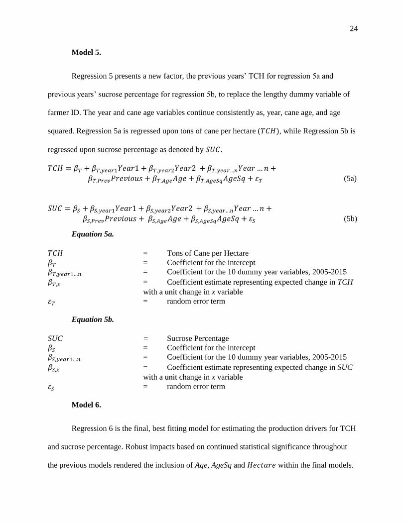
Model 5. ................................................................................................................................. 24

Model 6. ................................................................................................................................. 24

Results ........................................................................................................................................... 30

Descriptive Statistics ................................................................................................................. 30

Descriptive Statistics by Year. ............................................................................................... 31

Tons of Cane per Hectare Statistics. ...................................................................................... 31

Sucrose Percentage Statistics................................................................................................. 32

Temperature and Precipitation Statistics. .............................................................................. 32

Model 1: Table 4 and 5 ............................................................................................................. 33

Year. ...................................................................................................................................... 33

Hectare Classification: Small, Medium, Large. .................................................................... 34

Cane Age. .............................................................................................................................. 35

Model 2: Table 6 and 7 ............................................................................................................. 35

Hectares Harvested. ............................................................................................................... 35

Model 3: Table 8 and 9 ............................................................................................................. 36

Hectares Harvested and Hectares Harvested Squared. .......................................................... 36

Model 4: Table 10 and 11 ......................................................................................................... 37

Farmer Identifier. ................................................................................................................... 37

Model 5: Table 12 and 13 ......................................................................................................... 38

Previous Years’ Performance. ............................................................................................... 38

Previous Years’ Production. .................................................................................................. 39

Model 6: Table 14 and 15 ......................................................................................................... 39

Climatic Effects. .................................................................................................................... 39

Marginal Effect of Hectares Harvested on Production and Revenue. ................................... 42

Marginal Effect of Cane Age on Production and Revenue. .................................................. 43

Climatic Scenarios..................................................................................................................... 45

Conclusion .................................................................................................................................... 49

Discussion ..................................................................................................................................... 50

Tables ............................................................................................................................................ 53

Figures........................................................................................................................................... 69

References ..................................................................................................................................... 88

Appendices .................................................................................................................................... 93

Appendix 1 ................................................................................................................................ 93

Appendix 2 .............................................................................................................................. 104

1

Introduction

Sugar cane is the largest industry in Eswatini, in terms of share of Gross Domestic Product

(GDP), with approximately 400 million US$ revenue per year (Eswatini Sugar Association, 2017).

Approximately 16% of the total workforce is directly or indirectly employed through the sugar

cane industry, which illustrates its crucial social and economic presence in the wellbeing of

Eswatini (Eswatini Sugar Association, 2016). In 2016, it was estimated that the Kingdom of

Eswatini (KoE) had the highest national HIV-infected prevalence rate in the world with 27.2% of

adults infected (World Health Organization, 2017). Due to the high manual labor requirements of

agricultural production, loss of productivity from illness associated with HIV has been estimated

to be detrimental on the yields and earning abilities of infected households (Topouzis, 2003). Sugar

cane producers have also faced the recent challenges of high variability in both the timing and

amount of total rainfall which has lowered yield potential and increased yield variability amongst

both staple and cash crops (National Disaster Management Agency, 2016). In the face of both

variable weather patterns and vulnerability of smallholder farmers through losses of labor

productivity, Eswatini strives for solutions through research as the kingdom’s economy is based

on agriculture, specifically sugar cane production.

Although the HIV rate has fallen since 2005, from 28.3% of the adult population, it is

estimated there are still 220,000 individuals living with HIV in the country (World Health

Organization, 2017). High HIV/AIDS levels have been linked to high losses in productivity and

lowered household incomes, with a study in Nigeria showing that an average of 1,004 man-

hours/year are lost due to HIV/AIDS related illness and 4,630 average man-hours/year in caring

for household members that are ill (Yusuf & Purokayo, 2012). Another study within Uganda,

demonstrated that due to lost labor, loss of knowledge capital, and increased dependency burdens

2

76% of households were producing less agricultural products within the last 10 years due to HIV

(Topouzis, 2003).

Unlike the sugar cane industry in high-income countries such as the United States and

Australia, which relies entirely on mechanical harvesters, sugar cane production within Eswatini

requires intensive manual labor, with most producers still harvesting cane by hand (“Royal

Swaziland Sugar Corporation - Operations,” n.d.; United Nations Conference on Trade and

Development, 2000). Multiple studies have shown that as a result of working sugarcane by hand,

laborers can expect significant body mass drops from fluid loss, dehydration, and over exertion

that negatively impact even healthy worker’s performance (Christie, Langston, Todd, Hutchings,

& Elliott, 2008; Sanders & McCormick, 1993).

The social impacts of HIV/AIDS are exemplified by shifts in the labor market, as the most

impacted population are of working age (15-49) and represent a direct impact on individuals’

livelihood capabilities through changes such as increased dependency burdens and loss of

productivity (Food and Agriculture Organization & Office of Evaluation, 2011;

Ulandssekretariatet LO/FTF Council, 2012). The risks of productivity losses and decreased

earning potential disproportionately influence the rural residents who are likely to be involved in

agricultural work, with 13.3% of the employed rural population working in the formal agriculture

market (Economic Census 2011: Phase 1 Report, 2011; Falola & Jean-Jacques, 2016; Food and

Agriculture Organization & Office of Evaluation, 2011). In addition, over 70% of Eswatini’s

population rely on subsistence farming demonstrating the breadth of impact of weather on the

informal agricultural market and food security as well (Food and Agriculture Organization of the

United Nations, n.d.; Masuku, Kibrige, & Singh, 2015).

3

Rural communities are especially inflicted by negative consequences from HIV/AIDs due

to lack of access to health services, dependency on subsistence farming, and high risk of food

insecurity (Masuku et al., 2015; Topouzis, 2003). Eswatini’s rural community is particularly

affected by productivity losses from HIV/AIDS, with a 9% decrease of rural labor force

participation rate from 2007 to 2010, compared to only a 4% decrease in the urban areas (Ministry

of Labour and Social Security, 2010). In addition, the 51% rural unemployment rate is double that

of the urban rate at 23%, demonstrating the presence of additional challenges in rural areas

(Ministry of Labour and Social Security, 2010). The impact of the HIV/AIDS epidemic manifests

across all sectors of the economy through falling life expectancy, weakened social structures,

decreased productivity, and the loss of immeasurable human capital (Jahan, 2016; Lule, Haacker,

& World Bank, 2011; Muwanga, 2004; Watkins, 2006; Yusuf & Purokayo, 2012). Small-scale

sugar cane producers, defined as under 50 hectares by the Eswatini Cane Growers Association, are

often the hardest hit by HIV/AIDS as they traditionally rely on family labor more than hired labor.

Apart from infectious disease, recent climatic events within Eswatini have caused a 16%

reduction in sugar output in Eswatini (Eswatini Sugar Association, 2016). In 2015/16 the El Niño

drought was the worst drought Eswatini has experienced since 1992 (SEPARC, 2018). In total

nominal monetary terms, the drought cost Eswatini conservatively US $306.8 million, representing

a 7.01% of Eswatini’s GDP in 2016 or 18.58% of government expenditure in 2016 (SEPARC,

2018). However, even with extensive experience from past droughts in 2009/10, 2007, 2001, and

1992, the country is still struggling to cope better with the effects of drought with respect to

economic stability, food price stability and food security. Droughts hit Eswatini particularly hard

because of its reliance on surface water (mainly rivers) to provide irrigation for cash and staple

crops. Given that Eswatini is a relatively small country and droughts that effect it also have high

4

correlations with South African droughts, and the fact that Eswatini relies so heavily on imported

food from South Africa can pose food security issues.

The implication is that as droughts become more frequent regionally, their impact on the

Eswatini economy could be severe, particularly on rural livelihoods who rely on substance

agriculture (SEPARC, 2018). In July of 2016, the Eswatini Vulnerability Assessment Report

indicated that more than half of the population (638,251 people) in the country required livelihood

support, mainly in the form of food aid due to the El Niño drought. Droughts and variable weather

patterns will only continue to increase in frequency and magnitude (Intergovernmental Panel on

Climate Change (IPCC), 2007). The significance for Eswatini is that yields from rain-fed

agriculture could fall by up to 50% by 2020. Threatening the livelihoods of the rural poor, a

majority of whom earn their living through subsistence agriculture (Intergovernmental Panel on

Climate Change (IPCC), 2007, 2014).

For the 2016/17 season, the rainfall from the long-term mean was down a national total of

450 millimeters (mm) (Eswatini Cane Growers Association, 2017). Specifically, the rainfall

received for sugar cane producers in the Mhlume and Big Bend was 40% lower than the long term

means (Eswatini Cane Growers Association, 2017). In 2016, Eswatini Sugar Association (SSA)

cited compromised water availability as a negative factor in the short and medium term of the

sugar cane industry due to lowered water availability and rationed irrigation for sugar cane

producers (Eswatini Sugar Association, 2016). According to the SSA’s future of the Eswatini sugar

industry outlook, water shortages caused by changes in traditional rainfall patterns was cited as

one of the top ten risks to the sugar cane industry (Eswatini Sugar Association, 2016). Knox et al.

(2010) simulated possible outcomes based on historical Eswatini weather data, predicting that the

5

existing irrigation structures will fail to maintain the current levels of production even when

assuming unconstrained water availability.

In the case of Mhlume specifically, the ability for smallholder farmers to pay for water

rights is vulnerable. This leads to an inability to provide on-demand irrigation for their sugar cane

crops, potentially exasperating the effects of extreme weather events within this region.

Discussions led by Dr. Mkhwanazi within the Eswatini Economic Conference (2017) discussed

the need for improved water management techniques, as poor governance of irrigation was

identified as a potential threat to sustainability for agriculture in Eswatini.

The sugar cane industry is the foundation of the agricultural economy in Eswatini,

producing over half of the total annual agricultural production output, illustrating the risks for the

nation from detrimental climatic changes (Sikuka & Torry, 2017; United Nations Conference on

Trade and Development, 2000). Because of the drought and extreme heat events effect on

agricultural output, over 30,000 people faced food shortages between 2014-2016 and 75% of

households entered the 2016-2017 planting season with depleted food stocks in Eswatini

(Government of Eswatini, UN Office for the Coordination of Humanitarian Affairs, & UN Country

Team in Eswatini, 2016). As climate changes increases the frequency and intensity of extreme heat

events and alters traditional rainfall timing and amounts the sugar cane industry in Eswatini could

face long-run sustainability issues in terms of profitability.

Sugar Cane Production in Eswatini

Sugar cane is the main livelihood of the majority of the agricultural community within

Eswatini. The industry contributes to roughly 35% of the private sector employment (Eswatini

Sugar Assocation, 2016). Since 2014, the El Nino weather pattern has adversely affected the entire

agricultural community in Eswatini with overall food insecurity increasing from 3% in 2014 to

23.5% in 2015. The recent changes in rainfall, both in terms of timing and total amount, places up

6

to 70% of the population depending on rain-fed agriculture at the risk of becoming food insecure

(National Disaster Management Agency, 2016). Due to the fact that most sugarcane producers

work small farms, at less than 50 hectares harvested, yield variability caused by changing weather

patterns can greatly impact the profitability and livelihoods of these small-scale producers

(Eswatini Sugar Association, 2016). Although smallholder farmers are crucial to the growth of the

sugar cane industry within Eswatini, they face a disproportionate amount of challenges associated

with profitability. Access to inputs have been a large constraint for the smallholders within the

sugar industry, as many of these farmers do not have timely access and pay relatively higher prices

than larger farms (Eswatini Cane Growers Association, 2017). The SSA requires certain disease

control measures, as well as a predetermined harvest schedule and often smallholder farmers do

not have access to inputs due to high costs, lack experience, or lack business skills that hinder

proper compliance with the mills requirements (Masuku, 2011). The SSA provides marketing,

advisory, and technical services to farmers to support adherence to these guidelines, as the

guidelines are crucial to maintaining high quality output.

In 2016, sugar cane production accounted for approximately 60% of the total national

agricultural output and contributed to 10% of the kingdom’s total gross domestic product (GDP)

(Sikuka & Torry, 2017). One of the greatest vulnerabilities agricultural producers face is the

impact of weather volatility upon crop yields due to the inability to predict or mitigate climatic

risk. Sugar cane plants often have diminished yields due to suffering damage during crucial stages

of development from exposure to recent adverse weather conditions. Drought is a major factor

damaging sugar cane specifically due to the heightened requirement for consistent water supply in

the vegetative stage of the plants life-cycle (Zingaretti, Rodrigues, da Graça, Pereira, & Lourenço,

2012). Drought is partially mitigated by the fact that in Eswatini all sugarcane is irrigated. Extreme

7

heat events have been cited to hinder vegetative growth and sucrose accumulation, causing

diminished economic returns (Hasanuzzaman, Nahar, Alam, Roychowdhury, & Fujita, 2013).

Grower payment in Eswatini is based on both the volume of cane delivered to the mill, as well as

the amount of sucrose contained in the cane harvest. According to studies by Glasziou and Hatch

(1963), there is a negative correlation between the rate of stalk elongation and the rate of change

of sugar content due to the competition for the available photosynthate, complicating profitability

and climatic effect estimations on sugar cane producers (Glasziou, Bull, Hatch, & Whiteman,

1965; Hatch & Glasziou, 1963).

After planting, during the vegetative stage, extreme temperatures over 35°C can reduce

total cane biomass yields, which ultimately decrease producer earnings (Ebrahim, Zingsheim, El-

Shourbagy, Moore, & Komor, 1998; Moore & Botha, 2013). Sucrose formation, after the

vegetative state, is even more complex as colder temperatures are desirable unless they fall below

0°C which can negatively affect the sucrose content, by inhibiting transport of sucrose from the

leaves to the stalk (Ebrahim et al., 1998). While irrigation is necessary, at least in the Eswatini

context, for cane production, late rains during the sucrose stage can negatively impact the

percentage of sucrose (as the plant takes up water and thus dilutes the sucrose content) and thus

reduces producer profits (Gowing, 1977, as cited in, Blackburn, 1984). As weather patterns

become more extreme and less predictable this complex relationship between weather and

profitably poses new challenges for the Eswatini sugar industry and the large percentage of the

Eswatini population who rely on agriculture for their livelihoods.

Understanding the current state of global and regional climate change and its role in future

crop production in Eswatini is pivotal in ensuring livelihoods and ensuring food security (Zhao &

Li, 2015). Eswatini’s drought beginning in 2014 and 2015 has been linked to a decrease in food

8

security for a number of vulnerable communities, such as small holder farmers, rural households,

and those suffering from HIV/AIDS (Pound, Michicels, & Bonaficio, 2015). It is crucial for plant

breeders to focus on developing improved sugar cane varieties sculpted to this new global

environment. Cultivars should be tailored to be drought resistant as well as able to sustain

prolonged heat above the current temperature thresholds (Zingaretti et al., 2012). The development

of improved data and analysis on topics such as climate change, agricultural production, and rural

development will support the government’s ability to effectively assess the need for policy and

better inform decision makers concerning food security and energy sector development (Bioenergy

and Food Security Projects & FAO, 2013).

Problem Statement

Using on the field data provided by the SSA for 454 individual sugarcane producers from

2004-2015, coupled with location specific climatic data, this study provides a unique platform for

estimating the drivers of production for sugar cane farmers in Eswatini. The goal of this study is

to first, estimate if revenue per hectare is a function of farm size. Given the lack of extension

services throughout Africa, one fear is that large producers may have an inherent advantage in that

they can afford crop consultants, higher levels of mechanization and inputs such as inorganic

fertilizer. If larger farms can more easily mechanize then it’s likely the effects of HIV, in terms of

lost labor and reduced labor efficiency, would affect smallholder producers more in regard to

output per hectare. The government of Eswatini has made a concerted effort to reach out to small

and medium size sugar cane producers, which range from 0-50 and 50-1000 hectare farms,

respectively and provide extension services in an effort to increase production profitability.

Currently, there has not been research regarding the relationship between farm size and sugar cane

production. The findings of this study will provide the Eswatini government with important

9

information since farm size is related to revenue per hectare. This is imperative given that sugar

cane plays such a prominent role in the Eswatini economy and developing a relationship between

farm size and production per hectare could drive a more granular investment into specific areas of

extension research.

Second, given the unprecedented drought of the last decade this study set out to estimate

the effects of extreme temperatures and drought on biomass growth (TCH) and sucrose production

stages, which are the drivers of revenue. This study provides insights for sugar cane breeding

efforts, public policy, and agricultural decision making related to climate change in Eswatini. Our

findings provide opportunities for the international sugar cane producing community to intensify

research efforts to increase resistance to heat stress during focused developmental stages. A greater

understanding of extreme weather events is also needed to further Eswatini’s ability to forecast the

potential impacts of climate change on sugar cane yields. Further research such as this study

provides attention to improving specifications of the magnitude, duration, and frequency of

extreme weather events.

Literature Review

Eswatini Sugar Cane Agricultural Cycle

Factors influencing the physiological maturity of sugar cane have been studied for

decades. Weather effects on sugar cane vary according to the length, extent, and during which

phase of development. A background review of Eswatini agricultural cycle and abiotic stressors

on sugar cane is discussed in this next section.

During the sugar cane agricultural cycle two main phases occur: biomass growth and

sucrose accumulation (Ebrahim et al., 1998). In Eswatini, the autumn planting date occurs on

February 1st. Biomass growth is referred to as Season 1 throughout this study and occurs from

10

planting for 270 days. In Eswatini, season 1 is from February 1-October 28. Sucrose

accumulation occurs after tiller elongation is completed and sucrose content accrual begins from

day 271 until harvested. Season 2 in Eswatini lands from October 29-April 1, with estimated

harvest date at April 1st.1

There are two main planting seasons, autumn and spring, for sugar cane in Eswatini, with

the spring plant occurring on July 1 and the Autumn plant on February 1. The autumn replant

occurs after summer rains and spring replant happens when the temperatures rise after the winter

months, since cooler temperatures have a negative effect on cane germination and growth (N.

Dlamini, personal communication, June 12, 2017). The production guide for South Africa states

that the optimal time for planting is during the autumn replant if sugar cane is irrigated (Ebrahim

et al., 1998). As all sugar cane throughout Eswatini is irrigated, the autumn replant (February 1)

is the schedule this study’s seasons are based on. Although the overarching seasonal pattern of

February 1st-April 1st is followed, each individual farmer determines exactly when to plant and

harvest his/her own crop according to the weather conditions as well as, fallow requirements,

service provider(s) schedule, planting material availability, etc. (S. Nkambule, personal

communication, June 13, 2017).

Due to the versatility of planting dates by grower, the harvest of sugar cane has a broad

range, from April-December (S. Nkambule, personal communication, June 12, 2017). Harvesting

is generally completed during the dry period when the stalks contain the maximum amount of

sucrose. As much of the cane as possible is harvested at twelve months of age, but since the

harvesting period runs for nine months, the age varies according to the environmental conditions

1 Planting (February and July) and Harvesting (April-December) dates based on personal

communications with Sipho Nkambule, June 12, 2017.

11

such as precipitation and temperature. Although frost and prolonged cold temperature is the most

detrimental to sugar cane yields in terms of temperature damage, this extreme is not seen in

Eswatini and is therefore not a factor impacting yield in this region (N. Dlamini, personal

communication, June 12, 2017). High temperatures impact both biochemical and physiological

processes, and in combination with limited water, can cause depleted yield (N. Dlamini, personal

communication, June 12, 2017).

Studying heat stress on plants, specifically tropical plants, has become crucial in

agronomic research due to the impending threat of increasing climate temperatures. Damage

from high temperature stress was observed in sugar cane through necrosis, the rolling and drying

of leaves on leaf-tip and margins (Srivastava et al., 2012, as cited in, Hasanuzzaman et al., 2013).

The necessity to maintain high yields of crops has encouraged many studies on heat tolerance to

narrow in to the molecular level impacts of temperature. Crop plants can induce gene expression

and metabolite synthesis that adapt the plant to higher temperatures, and thus creating a higher

tolerance to this undesirable abiotic stressor. Plants can tolerate heat stress by creating signals

that change the metabolism of the plant, but of course, this only works to a certain extent of

stress. Researchers have not found a specific gene responsible for plant adaptability to heat but

have determined that it is a conglomeration of biological responses. Plants accumulate different

metabolites (antioxidants, osmoprotectants, heat shock proteins, etc.) and metabolic pathways,

with certain processes being activated under heat stress. Investigating these interlinked responses

are a crucial step to developing heat stress tolerant plants. Depending on the duration and extent

of extreme temperature, plant response to heat can impact the efficiency of enzymatic reactions,

RNA species, and create metabolic imbalances, and even cause cell death (Hasanuzzaman et al.,

2013).

12

Abiotic stressors impact the plant development differently during these phases, and so the

structure of this paper breaks down the impact of temperature and other variables for both

seasons. First, the effect of extreme heat and cold on biomass development in season 1 is

evaluated and then the influences of conditions for sucrose accumulation in season 2.

Season 1: Biomass Growth.

For the first 270 days, the sugar cane is growing through tillering and elongation. Tillering is

the physiological process of repeated underground branching from compact nodal joints of the

primary shoot (“Grand Growth phase,” n.d.). This provides the appropriate number of stalks

required for a good yield (Ebrahim et al., 1998). If sugar cane is grown in full sunlight, there are

thicker and shorter stalks, broader and greener leaves, greater rate of tiller production. If exposed

to sunlight all day, there is more dry matter produced (Martin & Eckart, 1933, as cited in,

Glasziou, Bull, Hatch, & Whiteman, 1965). The more time elapsed into the adult stage, the larger

the impact temperature has on plant and stalk growth (Glasziou et al., 1965).

During the biomass growth stage, cold weather has the most significant negative impact on

the ability for sugar cane to grow, as there is no growth (biomass production) below 12 or 15

degrees (Verret & Das, 1927; Sartorius, 1929; Ryker & Edgerton, 1931, as cited in, Ebrahim et

al., 1998). In addition to growth, extremely cold temperatures (15℃) also had an impact on the

shoot and root system with an 85% decrease of ratio from moderate temperature (27 ℃)

according to a study by Ebrahim (1998). Within the same study, plants grown at 27℃ had the

highest number of internodes, in comparison to those grown at 15℃ and 45℃ degrees,

throughout the growth period. Total biomass production was 1/2-1/3 less at 45℃, in comparison

to plants grown at 15℃ and 27℃, showing that extreme temperatures are not optimal for

biomass growth (Ebrahim et al., 1998).

13

Another study by Moore found that although leaf and tiller emergence increase up to 38℃

compared to those at 33℃, photosynthetic rate reduces past this point, indicating that extended

periods of time with warm temperatures could be detrimental (Moore & Botha, 2013; Blackburn,

1984). Warmer temperatures are required for the growth stage but increasing temperature above

the threshold of 35℃ hinders growth and is seen by a physically wilted cane with a lack of

growth occurring regardless of water supply (Moore & Botha, 2013). Extremely warm

temperatures can also impact sucrose content with any temperature higher than 35℃ resulting in

a limitation of photosynthesis and thus hindering sucrose accumulation (Hasanuzzaman et al.,

2013). The reduced growth rate under high temperatures have been attributed to a decrease in net

assimilation rate (NAR) within sugar cane (Srivastava et al., 2012, as cited in, Hasanuzzaman et

al., 2013).

A study by Das determined that the optimum temperature for dry matter for sucrose

production and concentration in the stalk is 30℃. Sugar yields also correlate well with day

degrees that are summed above 18 or 21 degrees (Das, 1933, as cited in, Glasziou et al., 1965).

Clements later confirmed that during the juvenile stage, the optimum temperature for plant and

stalk growth is 30℃, with sugarcane producing the highest sugar yields at growth temperatures

between 25-35℃ (1980, as cited in Ebrahim et al., 1998).

Season 2: Sucrose Accumulation.

For high yielding sugar cane sucrose accumulation, also referred to as ripening, must occur.

In short, sucrose accumulation ensues when sucrose is transported through the phloem from the

leaves towards the shoot and is accumulated in storage organs (Hatch & Glasziou, 1963).

Exporting sucrose from the leaves to the stalk of the sugar cane is subdued during low

temperatures, indicating that translocation is very sensitive to cooler temperatures (Ebrahim et

14

al., 1998). Gowing conducted a study in Iran and confirmed that the process of sucrose

accumulation is sensitive to high levels of rainfall and requires that temperature does not dip

below 10 degrees. A decrease in temperature below 10 degrees can cause irreparable cell damage

in the sugar cane (1977, as cited in, Blackburn, 1984).

Deressa explores how warmer temperatures during sucrose accumulation are not optimal for

sugar cane. If temperature is raised to 45℃, there is an elevated leaf respiration which causes a

reduction in the amount of available sugar for translocation. The increased respiration causes

lower sucrose concentration in the internodes of plants grown at 45℃ than at 15℃ or 27℃,

showing that high temperatures have a negative impact on sucrose content. In other studies, it

has been postulated that translocation from leaves to other parts of the plant is faster at lower

temperatures, confirming the theory that higher temperatures decrease yield in sugar cane. The

failure of the plants to store sugars at a high temperature is because the available photosynthate

for growth is being utilized. The photosynthate causing growth in the sugar cane is not

supportive for sucrose accumulation (Deressa, Hassan, & Poonyth, 2005).

Climate Change Impacts on Sugar Cane Production in Southern Africa

The impact of changing weather patterns has been studied several times in relation to

sugarcane production (Inman-Bamber & Smith, 2005; Knox, Rodríguez Díaz, Nixon, &

Mkhwanazi, 2010; Reinhard, Knox Lovell, & Thijssen, 2000; Zhao & Li, 2015). Zhao examines

the effects of climate change in the top ten sugar cane producing countries, finding that the

greatest yield variations occurring in developing countries across years (1973-2013) in locations

of unpredictable rainfall and temperatures (Zhao & Li, 2015). Low profits for sugar cane

producers in these regions are vulnerable due to low cane price, high costs of production due to

inputs (Zhao & Li, 2015). The study concluded that physiologically the most problematic

15

situation for sugar cane production is intense extreme climatic events occurring more frequently,

requiring new sugar cane cultivars bred for heat and drought resistance (Zhao & Li, 2015).

In one study by Knox, the CANEGRO model simulated several possible outcomes of

climate change on sugarcane production in Eswatini. A focus of the study was to assess the

impact on resource availability and water demand, which accounts for both irrigation abstraction

and crop production. It was found that there would be a 20-22% increased need for irrigation

from the baseline to continue with the current optimal levels of production (Knox et al., 2010).

Currently, all Eswatini sugarcane is irrigated as it is crucial to the production process (Inman-

Bamber & Smith, 2005). A majority of the water for Eswatini agriculture (96%) is currently used

for sugarcane production (Matondo, Graciana, & Msibi, 2004, as cited in, Knox et al., 2010).

Both modelling and production factors help to evaluate the efficiencies involved within a

profitable and productive sugarcane industry (Keating, Robertson, Muchow, & Huth, 1999;

Reza, Riaza, & Khan, 2016; Thabethe, 2013). Within Keating’s research, the use of the

modelling system, APSIM framework, within the sugarcane industry was evaluated. The goal of

the article was to simulate sugarcane crop to use a whole systems approach to production. The

authors hoped to increase the ability of researchers to evaluate productivity of sugarcane. In

conclusion, the article confirmed that this modelling system is adequate for observing most

physiological performance indicators of crops over a variety of production scenarios (Keating et

al., 1999).

Eswatini Sugar Cane Industry

The SSA manages all exported raw sugar produced in Eswatini. World sugar cane

production has tripled in the last 41 years due to increasing demand for this product (Zhao & Li,

2015). The two main markets for Eswatini 's export sugar include the South African Customs

16

Union (SACU) and the European Union (EU). SACU accounts for 45-70% of the sugar sales,

and the EU around 24-55%, although sales to the EU have fallen in recent years due to low

prices (Sikuka & Torry, 2017).

A general review of Sub Saharan Africa’s sugar cane production discovered diverse

methods of production, scale, and industry models. The study found that to best discuss the

environmental, social, and technical impacts of the industry, the evaluation must be context

specific. Ultimately, the review did not conclude with a good/bad or sustainable/unsustainable

consensus of the sugar cane industry within the Sub-Saharan region. Instead, suggesting a multi-

disciplinary analysis and planning for context-specific industries as crucial for encouraging

responsible sector sustainability. This synergistic approach, including various scales and

disciplines, is particularly crucial for water management and livelihoods for farmers within the

industry (Hess et al., 2016).

Another challenge for the industry, is presented as the need for research within the

specific contexts to evaluate the industry model’s ability to create equitable economic growth for

all those involved. The impacts of sugar cane are widespread across social and environmental

spheres with a high level of infrastructure required for irrigation, mills, and other factors (Hess et

al., 2016). Looking at smallholder sugar cane growers specifically, brings to the forefront the

potential challenges for this crucial segment of Eswatini’s sugar cane industry.

Smallholder Sugar Cane Grower Challenges

A South African case study evaluated various types of efficiencies within the sugarcane

sector by gathering information on farmer characteristics such as farmer education, access to

extension/credit, and market access for improved technologies. The results showed that small-

scale farmers were lacking efficiencies in all types tested; technical, allocative, and cost. It was

17

found that there was a need for better relationships between agricultural producers and sugar

cane mills. The author suggests technical guidelines for small farmers as an incentive for

punctual delivery of high quality sugar cane (Thabethe, 2013).

A study in Bangladesh found that outdated production practices, lack of adequate labor,

and low-quality sugar harvests are factors that contribute greatly to low productivity and

profitability in sugar mills (Reza et al., 2016). In addition, farmers were not reaching their

optimum production levels due to many reasons including, credit shortages, early or late

harvests, environmental resistance, and late planting. The results concluded that lack of proper

training, inadequate supply of inputs, and extended harvest periods were the major constraints

for producer profitability (Reza et al., 2016).

Masuku used personal interviews with smallholder farmers and representatives of farmer

cooperatives/associations’ to analyze the determinants of performance of the cane growers in the

sugar industry in Eswatini (Masuku, 2011). Using multiple linear regression, Masuku analyzed

the impact of several factors on the profitability of the farmer. The results determined the

profitability of the farmers was positively affected by several factors including; the yield per

hectare, sucrose content, and changes in production quotas’. Farmer experience negatively

impacted the profitability of sugar cane farmers. The author explains that this could be due to

confidence in ability and thus negligence in risk taking activities such as crop husbandry.

Distance to the mill was also found to be negatively influencing production performance.

Masuku concludes with suggestions that improving production efficiency and reduced input

costs could increase grower profits (Masuku, 2011).

An examination of smallholder sugar cane growers in Eswatini was conducted to

understand the relationship between social and economic aspects, as well as the influence of

18

agricultural development policies surrounding the industry (Terry & Ogg, 2016). The authors

highlight the crucial role of the sugar industry for Eswatini’s economy and focused especially on

the increasing importance of smallholder farmers within the profitability of this industry. The

review studies the evolution of the industry from focuses on benefits for the elite, to widespread

livelihood improvements for rural, small-scale farmers.

The shortage of skilled small-scale sugar cane producers is a concern that should be

addressed during the expansion and improvement of the sugar cane industry within Eswatini.

Three main areas of focus have been presented as potential solutions to lack of grower skills;

agronomic assistance through SSA extension, management abilities and industry knowledge, and

financial management skills (United Nations Conference on Trade and Development, 2000).

Currently, among the many long-term strategic objectives of the SSA is the objective of crop

protection and extension strategy. This strategy hopes to identify and prevent pests and diseases

and works to provide extension services to producers to develop skills to ensure the highest

possible yields (Eswatini Sugar Association, 2016).

Methodology

Data

Production data from 454 Eswatini farmers was received from the SSA in correspondence

with the Eswatini Economic Policy Analysis and Research Centre (SEPARC) for harvest years

2004-2015. At harvest, every sugar cane producer in Eswatini sells their yield to one of the three

processing mills: Simunye, Ubombo, and Mhlume. Each producer has been assigned a unique

identifier code (farmer ID), to ensure the privacy of the producers during the data analysis. The

mills use tons of cane per hectare harvested (TCH) and sucrose percentage to calculate the

payment for the purchase of each producer’s sugar cane. In addition to TCH and sucrose, other

19

variables such as farmer ID, area harvested, district, cane age at harvest, and farm size by

hectares for each year were included to help with analyses of production variability.

Originally, the dataset received from the SSA included data up to harvest year 2015-2016.

Due to a severe drought, the yield from this year had wide variability and thus would have

skewed the results and so this harvest year was eliminated from the dataset. To ensure that

adequate information for each farmer was available to draw results from, only farmers with more

than 5 observations were included in the analysis. This allows for at least 5 years of yield

statistics to each farmer ID. Due to the unlikely chance of uprooted crop or large acquisitions,

any farmers that increased or decreased the number of hectares harvested by larger than 50% its

size from the year before was not included in the dataset. Historical sucrose price (SZL E/ton of

sucrose) data was sourced from the SSA together with the grower revenue calculation equations.

Daily weather data was gathered for maximum, minimum, average temperatures, and

precipitation from aWhere. aWhere is a global agriculture focused model environment that

focuses on collecting data points to increase insight into agricultural and climatic trends

(“aWhere,” 2017). The weather dataset used within this study consisted of daily weather from

2008-2016 for districts Mhlume, Simunye, and Big Bend. Note that Big Bend is near the area of

the Ubombo milling site, and thus was used for Ubombo’s weather data. Precipitation was

measured by millimeters (mm) and all temperatures are reported in Celsius (℃).

Data Analysis

Initial data analysis included descriptive statistics based around the means and standard

deviations of variables based on yearly, district, and kingdom wide divisions. Multiple linear

regression models were used to estimate the effect of farm size, cane age, and climatic variables

on production through tons of cane harvested per hectare and sucrose percentage. By analyzing

20

the driving factors on sugar cane production, farm size and climatic variables can be pinpointed

for policy implications, as well as discovering areas in need of future research. Data was

analyzed in R Studio version 1.0.143, with regressions being run with the linear model (lm)

function inside of the package stats. Figures were created through R Studio function ggplot2 and

Microsoft Excel (Wickham, 2009).

Several regression models were analyzed through the systematic evaluation of each

variable’s robustness within the production estimates. Normality of means was assumed through

the Central Limit Theorem (n>30).. The dummy variables that are used as the reference within

the model intercepts are as follows: the Year 2004-2005, the District of Mhlume, and the Hectare

Class: Large. Initially, the production (and weather) data was divided by district (Mhlume,

Simunye, and Ubombo) to understand the production effects within each region of the kingdom.

A regression was calculated for all three districts and the pooled dataset for all of Eswatini within

each model, allowing for four regressions per model. The final models, Regression 6a and 6b,

were the result of the best fitting estimators to provide the most accurate representation of

production drivers within Eswatini.

Model 1.

Regression 1a and 1b includes Year, Med, Small, Age, AgeSq which represents; year

(2004-2015), hectare class medium dummy variable, hectare class small dummy variable, age,

age squared, respectively. Regression 1a is regressed upon tons of cane per hectare (TCH) while

Regression 1b is regressed upon sucrose percentage as denoted by SUC.

𝑇𝐶𝐻 = 𝛽𝑇 + 𝛽𝑇,𝑦𝑒𝑎𝑟1𝑌𝑒𝑎𝑟1 + 𝛽𝑇,𝑦𝑒𝑎𝑟2𝑌𝑒𝑎𝑟2 + 𝛽𝑇,𝑦𝑒𝑎𝑟…𝑛𝑌𝑒𝑎𝑟 … 𝑛 +

𝛽𝑇,𝑀𝑒𝑑𝑀𝑒𝑑 + 𝛽𝑇,𝑆𝑚𝑆𝑚𝑎𝑙𝑙 + 𝛽𝑇,𝐴𝑔𝑒𝐴𝑔𝑒 + 𝛽𝑇,𝐴𝑔𝑒𝑆𝑞𝐴𝑔𝑒𝑆𝑞 + 𝜀𝑇 (1a)

𝑆𝑈𝐶 = 𝛽𝑆 + 𝛽𝑆,𝑦𝑒𝑎𝑟1𝑌𝑒𝑎𝑟1 + 𝛽𝑆,𝑦𝑒𝑎𝑟2𝑌𝑒𝑎𝑟2 + 𝛽𝑆,𝑦𝑒𝑎𝑟…𝑛𝑌𝑒𝑎𝑟 … 𝑛 +

𝛽𝑆,𝑀𝑒𝑑𝑀𝑒𝑑 + 𝛽𝑆,𝑆𝑚𝑆𝑚𝑎𝑙𝑙 + 𝛽𝑆,𝐴𝑔𝑒𝐴𝑔𝑒 + 𝛽𝑆,𝐴𝑔𝑒𝑆𝑞𝐴𝑔𝑒𝑆𝑞 + 𝜀𝑆 (1b)

21

Equation 1a.

𝑇𝐶𝐻 = Tons of Cane per Hectare

𝛽𝑇 = Coefficient for the intercept

𝛽𝑇,𝑦𝑒𝑎𝑟1…𝑛 = Coefficient for the 10 dummy year variables, 2005-2015

𝛽𝑇,𝑥 = Coefficient estimate representing expected change in TCH

with a unit change in x variable

𝜀𝑇 = random error term

Equation 1b.

SUC = Sucrose Percentage

𝛽𝑆 = Coefficient for the intercept

𝛽𝑆,𝑦𝑒𝑎𝑟1…𝑛 = Coefficient for the 10 dummy year variables, 2005-2015

𝛽𝑆,𝑥 = Coefficient estimate representing expected change in SUC


𝜀𝑆 = random error term

Model 2.

Within Regression 2a and 2b hectare class dummy variable (𝑀𝑒𝑑, 𝑆𝑚𝑎𝑙𝑙) is replaced by

the continuous variable, hectares harvested, denoted by 𝐻𝑒𝑐𝑡𝑎𝑟𝑒. All other variables, Year, Age,

and AgeSq, remain the same as Regression 1. Regression 2a is regressed upon tons of cane per

hectare (𝑇𝐶𝐻), while Regression 2b is regressed upon sucrose percentage as denoted by 𝑆𝑈𝐶.


𝛽𝑇,𝐻𝑎𝐻𝑒𝑐𝑡𝑎𝑟𝑒𝑠 + 𝛽𝑇,𝐴𝑔𝑒𝐴𝑔𝑒 + 𝛽𝑇,𝐴𝑔𝑒𝑆𝑞𝐴𝑔𝑒𝑆𝑞 + 𝜀𝑇 (2a)


𝛽𝑇,𝐻𝑎𝐻𝑒𝑐𝑡𝑎𝑟𝑒 + 𝛽𝑆,𝐴𝑔𝑒𝐴𝑔𝑒 + 𝛽𝑆,𝐴𝑔𝑒𝑆𝑞𝐴𝑔𝑒𝑆𝑞 + 𝜀𝑆 (2b)

Equation 2a.







22

Equation 2b.







Model 3.

Regression 3a and 3b includes an additional variable, hectare harvested squared

(𝐻𝑒𝑐𝑡𝑎𝑟𝑒𝑆𝑞), to measure the non-linear aspects of farm size. All other right-side factors are the

same as before in Regression 2. Regression 3a is regressed upon tons of cane per hectare (𝑇𝐶𝐻),

while Regression 3b is regressed upon sucrose percentage as denoted by 𝑆𝑈𝐶.


𝛽𝑇,𝐻𝑎𝐻𝑒𝑐𝑡𝑎𝑟𝑒𝑠 + 𝛽𝑇,𝐻𝑎𝑆𝑞𝐻𝑒𝑐𝑡𝑎𝑟𝑒𝑆𝑞 + 𝛽𝑇,𝐴𝑔𝑒𝐴𝑔𝑒 + 𝛽𝑇,𝐴𝑔𝑒𝑆𝑞𝐴𝑔𝑒𝑆𝑞 + 𝜀𝑇 (3a)


𝛽𝑇,𝐻𝑎𝐻𝑒𝑐𝑡𝑎𝑟𝑒𝑠 + 𝛽𝑇,𝐻𝑎𝑆𝑞𝐻𝑒𝑐𝑡𝑎𝑟𝑒𝑆𝑞 + 𝛽𝑆,𝐴𝑔𝑒𝐴𝑔𝑒 + 𝛽𝑆,𝐴𝑔𝑒𝑆𝑞𝐴𝑔𝑒𝑆𝑞 + 𝜀𝑆 (3b)

Equation 3a.







Equation 3b.







23

Model 4.

Regression 4 eliminates the hectares harvested variables (𝐻𝑒𝑐𝑡𝑎𝑟𝑒, 𝐻𝑒𝑐𝑡𝑎𝑟𝑒𝑆𝑞) and replaces it

with the dummy variables for individual farmer identifier codes, as represented by

𝐹𝑎𝑟𝑚𝑒𝑟𝐼𝐷1 − 𝐹𝑎𝑟𝑚𝑒𝑟𝐼𝐷𝑘. There are 454 unique farmer ID’s, with IDM001 being the reference

farmer ID, and each are represented by 𝐹𝑎𝑟𝑚𝑒𝑟𝐼𝐷𝑘. The year and cane age variables remain as,

Year, Age, and AgeSq. Regression 4a is regressed upon tons of cane per hectare (𝑇𝐶𝐻), while

Regression 4b is regressed upon sucrose percentage as denoted by 𝑆𝑈𝐶.


𝛽𝑆,𝐼𝐷1𝐹𝑎𝑟𝑚𝑒𝑟𝐼𝐷1 + 𝛽𝑇,𝐼𝐷2𝐹𝑎𝑟𝑚𝑒𝑟𝐼𝐷2 + 𝛽𝑇,𝐼𝐷…𝑘𝐹𝑎𝑟𝑚𝑒𝑟𝐼𝐷. . 𝑘 + 𝛽𝑇,𝐴𝑔𝑒𝐴𝑔𝑒 + 𝛽𝑇,𝐴𝑔𝑒𝑆𝑞𝐴𝑔𝑒𝑆𝑞 + 𝜀𝑇 (4a)


𝛽𝑆,𝐼𝐷1𝐹𝑎𝑟𝑚𝑒𝑟𝐼𝐷1 + 𝛽𝑇,𝐼𝐷2𝐹𝑎𝑟𝑚𝑒𝑟𝐼𝐷2 + 𝛽𝑇,𝐼𝐷…𝑘𝐹𝑎𝑟𝑚𝑒𝑟𝐼𝐷. . 𝑘 + 𝛽𝑆,𝐴𝑔𝑒𝐴𝑔𝑒 + 𝛽𝑆,𝐴𝑔𝑒𝑆𝑞𝐴𝑔𝑒𝑆𝑞 + 𝜀𝑆 (4b)

Equation 4a.




𝛽𝑇,𝐼𝐷1𝐹𝑎𝑟𝑚𝑒𝑟𝐼𝐷1. . 𝑘 = 453 dummy variables for Farmer ID 1-454




Equation 4b.




𝛽𝑆,𝐼𝐷1𝐹𝑎𝑟𝑚𝑒𝑟𝐼𝐷1 … 𝑘 = 453 dummy variables for Farmer ID 1-454




24

Model 5.

Regression 5 presents a new factor, the previous years’ TCH for regression 5a and

previous years’ sucrose percentage for regression 5b, to replace the lengthy dummy variable of

farmer ID. The year and cane age variables continue consistently as, year, cane age, and age

squared. Regression 5a is regressed upon tons of cane per hectare (𝑇𝐶𝐻), while Regression 5b is

regressed upon sucrose percentage as denoted by 𝑆𝑈𝐶.


𝛽𝑇,𝑃𝑟𝑒𝑣𝑃𝑟𝑒𝑣𝑖𝑜𝑢𝑠 + 𝛽𝑇,𝐴𝑔𝑒𝐴𝑔𝑒 + 𝛽𝑇,𝐴𝑔𝑒𝑆𝑞𝐴𝑔𝑒𝑆𝑞 + 𝜀𝑇 (5a)


𝛽𝑆,𝑃𝑟𝑒𝑣𝑃𝑟𝑒𝑣𝑖𝑜𝑢𝑠 + 𝛽𝑆,𝐴𝑔𝑒𝐴𝑔𝑒 + 𝛽𝑆,𝐴𝑔𝑒𝑆𝑞𝐴𝑔𝑒𝑆𝑞 + 𝜀𝑆 (5b)

Equation 5a.







Equation 5b.







Model 6.

Regression 6 is the final, best fitting model for estimating the production drivers for TCH

and sucrose percentage. Robust impacts based on continued statistical significance throughout

the previous models rendered the inclusion of Age, AgeSq and 𝐻𝑒𝑐𝑡𝑎𝑟𝑒 within the final models.

25

In addition, each model improves the explanatory power and ability for policy implications, with

Model 6 best explaining the influences of farm size and climatic variables on production. The

best measurement of individual farmer’s management and production practices was previous

years’ TCH and sucrose percentage, as represented by 𝑃𝑟𝑒𝑣𝑖𝑜𝑢𝑠. Previously, Year was used in

Models 1-5 as a proxy for weather effects on production. Year was replaced by specific critical

thresholds and weather variables within Model 6 to better represent how the environment

influences the Eswatini grower’s yields and sucrose content. Model 6a, as regressed on TCH,

focuses on the critical threshold, Time above 35℃, as this critical threshold hinders biomass

growth resulting in lower cane weight. Regression 6b estimates the sucrose percentage of the

cane since sucrose accumulation occurs in the second season and is impacted by cold

temperatures and excessive precipitation. To better estimate the sucrose impacts, the elements

average minimum temperature and precipitation are included. Model 6 includes the best fitting

estimators, tested throughout Model 1-5, for cane age, farm size, and environmental factors on

TCH and sucrose percentage.

𝑇𝐶𝐻 = 𝛽0 + 𝛽𝑆,𝐴𝑔𝑒𝐴𝑔𝑒 + 𝛽𝑆,𝐴𝑔𝑒𝑆𝑞𝐴𝑔𝑒𝑆𝑞 + 𝛽𝑆,𝐻𝑒𝑐𝑡𝑎𝑟𝑒𝑠𝐻𝑒𝑐𝑡𝑎𝑟𝑒𝑠 +

𝛽𝑆,𝑃𝑟𝑒𝑣𝑖𝑜𝑢𝑠𝑃𝑟𝑒𝑣𝑖𝑜𝑢𝑠 + 𝛽𝑆,𝑇𝑎𝑏𝑜𝑣𝑒35𝑇𝑎𝑏𝑜𝑣𝑒35𝐶 + 𝜀𝑆 (6a)

𝑆𝑈𝐶 = 𝛽0 + 𝛽𝑇,𝐴𝑔𝑒𝐴𝑔𝑒 + 𝛽𝑇,𝐴𝑔𝑒𝑆𝑞𝐴𝑔𝑒𝑆𝑞 + 𝛽𝑇,𝐻𝑒𝑐𝑡𝑎𝑟𝑒𝑠𝐻𝑒𝑐𝑡𝑎𝑟𝑒𝑠 +

𝛽𝑇,𝑃𝑟𝑒𝑣𝑖𝑜𝑢𝑠𝑃𝑟𝑒𝑣𝑖𝑜𝑢𝑠 + 𝛽𝑇,𝐴𝑣𝑔𝑀𝑖𝑛𝐴𝑣𝑔𝑀𝑖𝑛 + 𝛽𝑇,𝑃𝑟𝑒𝑐𝑖𝑝𝑃𝑟𝑒𝑐𝑖𝑝 + 𝜀𝑆 (6b)

Equation 6a.



𝑇𝑎𝑏𝑜𝑣𝑒35𝐶 = Time (Degree Days) above 35℃




Equation 6b.


26


𝐴𝑣𝑔𝑀𝑖𝑛 = Average daily minimum temperature in season 2

𝑃𝑟𝑒𝑐𝑖𝑝 = Average daily precipitation in season 2




Marginal Effects.

The marginal effect equation was used to find the amount of change in production from a

one-unit change in hectares harvested squared and cane age squared. Note that since the one-unit

change was more applicable in this study, and not the instantaneous rate of change, the following

Equation 1 was used rather than the customary partial derivative. The analysis of variables,

hectares harvested squared and age squared (𝐻𝑒𝑐𝑡𝑎𝑟𝑒𝑆𝑞, 𝐴𝑔𝑒𝑆𝑞) was based upon the marginal

effect of the variable on TCH and sucrose percentage. Equation 1 demonstrates how one more

month of age influences yield (1a) and sucrose percentage (1b), while all other variables are held

constant. Equation 2 demonstrates how one hectare harvested effects TCH (2a) and sucrose

percentage (2b), while all other variables are held constant.

Equation 1. Marginal Effect of Age.

Equation 1 calculates the marginal effect, being the effect of a one unit change in cane

age and age squared on TCH (1a) and Sucrose percentage (1b). The equation allows for

measuring the impact of any cane age on production by simply changing the age within the

variable A. Note that Figure 18 and 19 uses coefficient estimates for cane age by month, 𝛽4, and

cane age squared, 𝛽5, derived from Model 6 for the marginal effect calculation as discussed

within the results section.

Marginal effect of Age on expected TCH = 𝛽4 + 2𝛽5𝐴 + 𝛽5 (1a)

Marginal effect of Age on expected SUC = 𝛽4 + 2𝛽5𝐴 + 𝛽5 (1b)

27

𝛽4 = Coefficient estimate representing the expected change in age variable with a

unit change in TCH, SUC.

𝛽5 = Coefficient estimate representing the expected change in age squared variable

with a unit change in TCH, SUC.

𝐴 = number of months of cane age

Equation 2. Marginal Effect of Hectares.

Equation 2 calculates the marginal effect of hectares harvested and hectares harvested

squared on TCH (2a) and sucrose percentage (2b). The equation can be calculated for farms of

all sizes to measure the impact of hectares harvested on production by modifying the number of

hectares within the variable H. Note that Figure 16 and 17 use coefficient estimates for hectares

harvested, 𝛽6, and hectares harvested squared, 𝛽7, derived from Model 3 for the marginal effect

calculations as discussed within the results section.

Marginal effect of Hectares on expected TCH = 𝛽6 + 2𝛽7𝐻 + 𝛽7 (2a)

Marginal effect of Hectares on expected SUC = 𝛽6 + 2𝛽7𝐻 + 𝛽7 (2b)

𝛽6 = Coefficient estimate representing the expected change in Hectare harvested

variable with a unit change in TCH, SUC.

𝛽7 = Coefficient estimate representing the expected change in Hectare harvested

Squared variable with a unit change in TCH, SUC.

𝐻 = number of hectares harvested

Producer Revenue. Equation 3.

Eswatini producers are paid according to the number of tons of cane per hectare and level

of sucrose percentage of the cane, which is calculated as sucrose produced. Farm revenue is then

calculated by including the price of sucrose in that year, denoted as ρ within the producer

revenue equation (3). The average sucrose price (SZL/ ton) from 2008-2015 was used to

calculate producer revenues (T. Dlamini, personal correspondence, April 9, 2018).

ℛ = 𝜌( 𝑇𝐶𝐻 ∗ 𝑆𝑈𝐶) (3)

28

ℛ = Producer revenue per ton

𝜌 = Sucrose Price; Swazi emalangeni/ton of sucrose ( 𝑇𝐶𝐻 ∗ 𝑆𝑈𝐶) = Sucrose produced (tons per hectare)


𝑆𝑈𝐶 = Sucrose Percentage

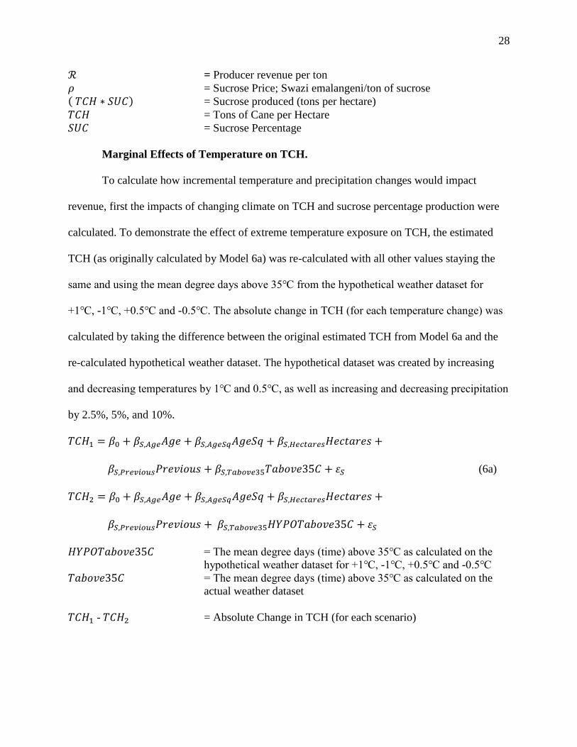
Marginal Effects of Temperature on TCH.

To calculate how incremental temperature and precipitation changes would impact

revenue, first the impacts of changing climate on TCH and sucrose percentage production were

calculated. To demonstrate the effect of extreme temperature exposure on TCH, the estimated

TCH (as originally calculated by Model 6a) was re-calculated with all other values staying the

same and using the mean degree days above 35℃ from the hypothetical weather dataset for

+1℃, -1℃, +0.5℃ and -0.5℃. The absolute change in TCH (for each temperature change) was

calculated by taking the difference between the original estimated TCH from Model 6a and the

re-calculated hypothetical weather dataset. The hypothetical dataset was created by increasing

and decreasing temperatures by 1℃ and 0.5℃, as well as increasing and decreasing precipitation

by 2.5%, 5%, and 10%.

𝑇𝐶𝐻1 = 𝛽0 + 𝛽𝑆,𝐴𝑔𝑒𝐴𝑔𝑒 + 𝛽𝑆,𝐴𝑔𝑒𝑆𝑞𝐴𝑔𝑒𝑆𝑞 + 𝛽𝑆,𝐻𝑒𝑐𝑡𝑎𝑟𝑒𝑠𝐻𝑒𝑐𝑡𝑎𝑟𝑒𝑠 +

𝛽𝑆,𝑃𝑟𝑒𝑣𝑖𝑜𝑢𝑠𝑃𝑟𝑒𝑣𝑖𝑜𝑢𝑠 + 𝛽𝑆,𝑇𝑎𝑏𝑜𝑣𝑒35𝑇𝑎𝑏𝑜𝑣𝑒35𝐶 + 𝜀𝑆 (6a)

𝑇𝐶𝐻2 = 𝛽0 + 𝛽𝑆,𝐴𝑔𝑒𝐴𝑔𝑒 + 𝛽𝑆,𝐴𝑔𝑒𝑆𝑞𝐴𝑔𝑒𝑆𝑞 + 𝛽𝑆,𝐻𝑒𝑐𝑡𝑎𝑟𝑒𝑠𝐻𝑒𝑐𝑡𝑎𝑟𝑒𝑠 +

𝛽𝑆,𝑃𝑟𝑒𝑣𝑖𝑜𝑢𝑠𝑃𝑟𝑒𝑣𝑖𝑜𝑢𝑠 + 𝛽𝑆,𝑇𝑎𝑏𝑜𝑣𝑒35𝐻𝑌𝑃𝑂𝑇𝑎𝑏𝑜𝑣𝑒35𝐶 + 𝜀𝑆

𝐻𝑌𝑃𝑂𝑇𝑎𝑏𝑜𝑣𝑒35𝐶 = The mean degree days (time) above 35℃ as calculated on the

hypothetical weather dataset for +1℃, -1℃, +0.5℃ and -0.5℃

𝑇𝑎𝑏𝑜𝑣𝑒35𝐶 = The mean degree days (time) above 35℃ as calculated on the

actual weather dataset

𝑇𝐶𝐻1 - 𝑇𝐶𝐻2 = Absolute Change in TCH (for each scenario)

29

Marginal Effects of Temperature and Precipitation on Sucrose Percentage.

To demonstrate the effect of changes in the average minimum temperatures on sucrose

percentage, the estimated percentage (as originally calculated by Model 6b), was re-calculated

with all other values staying the same, but using the mean average minimum temperature from

the hypothetical weather dataset for +1℃, -1℃, +0.5℃ and -0.5℃. To demonstrate the effect of

changes in precipitation on sucrose percentage, the estimated percentage (as originally calculated

by Model 6b), was re-calculated with all over values staying the same, but using the mean

average precipitation from the hypothetical weather dataset for -10%, -5%, -2.5%, 2.5%, 5%, and

10% changes in precipitation, with the mean minimum temperature constant at the values for the

hypothetical dataset for +1℃, -1℃, +0.5℃ and -0.5℃.

The absolute change in sucrose percentage (for each temperature and precipitation

change) was calculated by taking the difference between the original estimated sucrose

percentage from Model 6b and the re-calculated sucrose percentage based on the hypothetical

weather dataset values for minimum average temperature and precipitation.

𝑆𝑈𝐶1 = 𝛽0 + 𝛽𝑇,𝐴𝑔𝑒𝐴𝑔𝑒 + 𝛽𝑇,𝐴𝑔𝑒𝑆𝑞𝐴𝑔𝑒𝑆𝑞 + 𝛽𝑇,𝐻𝑒𝑐𝑡𝑎𝑟𝑒𝑠𝐻𝑒𝑐𝑡𝑎𝑟𝑒𝑠 +

𝛽𝑇,𝑃𝑟𝑒𝑣𝑖𝑜𝑢𝑠𝑃𝑟𝑒𝑣𝑖𝑜𝑢𝑠 + 𝛽𝑇,𝐴𝑣𝑔𝑀𝑖𝑛𝐴𝑣𝑔𝑀𝑖𝑛 + 𝛽𝑇,𝑃𝑟𝑒𝑐𝑖𝑝𝑃𝑟𝑒𝑐𝑖𝑝 + 𝜀𝑆 (6b)

𝑆𝑈𝐶2 = 𝛽0 + 𝛽𝑇,𝐴𝑔𝑒𝐴𝑔𝑒 + 𝛽𝑇,𝐴𝑔𝑒𝑆𝑞𝐴𝑔𝑒𝑆𝑞 + 𝛽𝑇,𝐻𝑒𝑐𝑡𝑎𝑟𝑒𝑠𝐻𝑒𝑐𝑡𝑎𝑟𝑒𝑠 + 𝛽𝑇,𝑃𝑟𝑒𝑣𝑖𝑜𝑢𝑠𝑃𝑟𝑒𝑣𝑖𝑜𝑢𝑠

+ 𝛽𝑇,𝐴𝑣𝑔𝑀𝑖𝑛𝐻𝑌𝑃𝑂𝐴𝑣𝑔𝑀𝑖𝑛 + 𝛽𝑇,𝑃𝑟𝑒𝑐𝑖𝑝𝐻𝑌𝑃𝑂𝑃𝑟𝑒𝑐𝑖𝑝 + 𝜀𝑆

𝐻𝑌𝑃𝑂𝐴𝑣𝑔𝑀𝑖𝑛 = The mean average minimum temperature in season 1 as

calculated on the hypothetical weather dataset for +1℃, -1℃,

+0.5℃ and -0.5℃

𝐻𝑌𝑃𝑂𝑃𝑟𝑒𝑐𝑖𝑝 = The mean precipitation in season 1 as calculated on the

hypothetical weather dataset for -10%, -5%, -2.5%, 2.5%, 5%, and

10% changes in precipitation

𝐴𝑣𝑔 𝑀𝑖𝑛 = The mean average minimum temperature in season 1 as

calculated on the actual weather dataset

30

𝑃𝑟𝑒𝑐𝑖𝑝 = The mean precipitation in season 1 as calculated on the actual

weather dataset

𝑆𝑈𝐶1 - 𝑆𝑈𝐶2 = Absolute Change in Sucrose percentage (for each scenario)

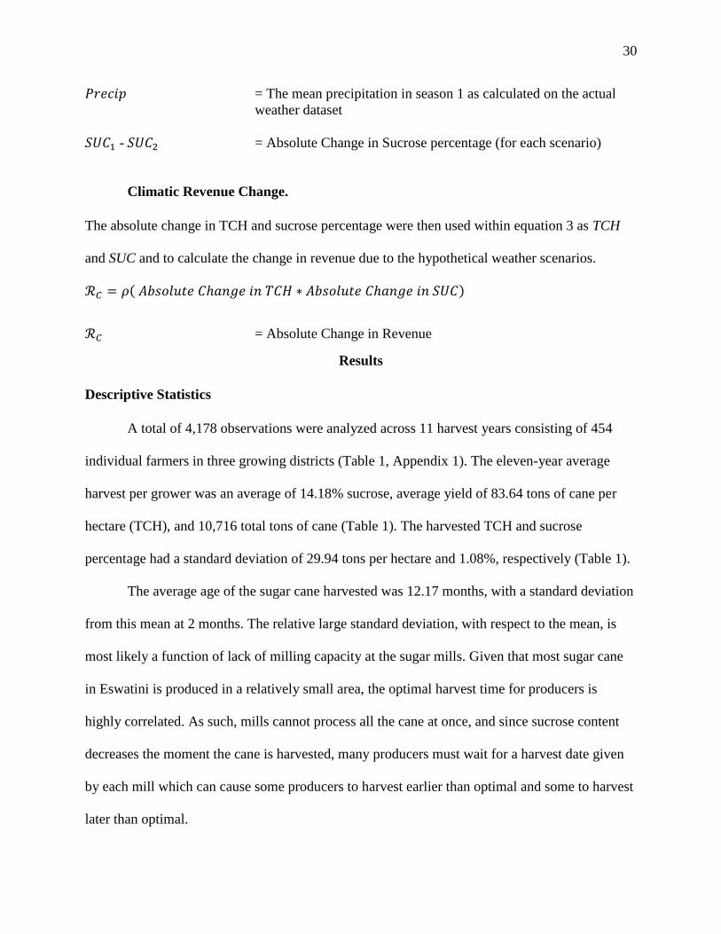
Climatic Revenue Change.

The absolute change in TCH and sucrose percentage were then used within equation 3 as TCH

and SUC and to calculate the change in revenue due to the hypothetical weather scenarios.

ℛ𝐶 = 𝜌( 𝐴𝑏𝑠𝑜𝑙𝑢𝑡𝑒 𝐶ℎ𝑎𝑛𝑔𝑒 𝑖𝑛 𝑇𝐶𝐻 ∗ 𝐴𝑏𝑠𝑜𝑙𝑢𝑡𝑒 𝐶ℎ𝑎𝑛𝑔𝑒 𝑖𝑛 𝑆𝑈𝐶)

ℛ𝐶 = Absolute Change in Revenue

Results

Descriptive Statistics

A total of 4,178 observations were analyzed across 11 harvest years consisting of 454

individual farmers in three growing districts (Table 1, Appendix 1). The eleven-year average

harvest per grower was an average of 14.18% sucrose, average yield of 83.64 tons of cane per

hectare (TCH), and 10,716 total tons of cane (Table 1). The harvested TCH and sucrose

percentage had a standard deviation of 29.94 tons per hectare and 1.08%, respectively (Table 1).

The average age of the sugar cane harvested was 12.17 months, with a standard deviation

from this mean at 2 months. The relative large standard deviation, with respect to the mean, is

most likely a function of lack of milling capacity at the sugar mills. Given that most sugar cane

in Eswatini is produced in a relatively small area, the optimal harvest time for producers is

highly correlated. As such, mills cannot process all the cane at once, and since sucrose content

decreases the moment the cane is harvested, many producers must wait for a harvest date given

by each mill which can cause some producers to harvest earlier than optimal and some to harvest

later than optimal.

31

The average farm size was 105 hectares, with a large standard deviation of 727 hectares.

The median is 5.67 hectares, indicating that there are more “small” farms than “large” farms. The

largest farm is 11,555 hectares, relatively much larger than the average of 105 hectares. Farm

size is classified by the Eswatini Sugar Cane Growers Association as being large when there are

over 1,000 hectares harvested, medium when 50-1,000 hectares harvested, and small when less

than 50 hectares harvested. Based upon this classification, this dataset includes a total of 454

farms with 74 large farms, 595 medium farms, and 3,509 small farms. In terms of numbers of

producers, this would seem to indicate that the sugar industry is predominately made up by small

scale farmers.

Descriptive Statistics by District.

Table 2 illustrates the differences between districts with respect to average farm size and

number of total producers. Mhlume is the largest district by number of observations with 3,072

followed by Ubombo at 853, and Simunye at 253 (Table 2). In contrast, Table 2 demonstrates

that the farm size is much smaller in terms of average hectares harvested in Mhlume (44), than in

both Ubombo (177) and Simunye (609).

Descriptive Statistics by Year.

Table 3 indicates that the 2014-2015 growing season has the highest number of hectares

harvested and in turn also the highest total tons of cane produced. The lowest volume of

production (hectares harvested) was during the 2004-2005 growing season, which was during a

drought (Table 3).

Tons of Cane per Hectare Statistics.

There are differences in yields by district with Mhlume, Simunye, and Ubombo

producing an average of 80.40, 94.13, and 92.23 TCH, respectively. Figure 1 demonstrates a

32

high level of variation of TCH between years across all of Eswatini. For example, the highest

producing year (in regards to TCH) was in 2005-2006 with more than 90 tons of cane per hectare

and the lowest producing year was in 2008-2009 at less than 75 tons (Figure 1). Figure 2

indicates that Simunye and Ubombo have a tendency for higher and more stable TCH yields with

averages around 90 TCH. Mhlume, in contrast, has a wide variation between years with TCH

ranging from 67 to 89 tons, and the highest producing year (2006-2007) does not even reach the

mean values of the other two districts, Simunye and Ubombo at 94.13 and 92.23 (Figure 2).

Using ANOVA testing within R, it was found that there are significant differences between the

districts’ TCH means (P<0.001). An explanation for this variation could be that out of the 3,072

observations from Mhlume, 2,799 of them are small farms. Small farms are most susceptible to

higher yield variation in Eswatini as they are less likely to be able to consistently afford inputs

and consulting services which can both enhance and smooth yields over time.

Sucrose Percentage Statistics.

Differences in sucrose percentages across districts were marginal. Across all districts

sucrose averaged 14%, with Mhlume averaging 14.29%, Simunye averaging 14.01%, and

Ubombo averaging 13.83% (Table 2, Figure 4). Using ANOVA testing within R, it was found

that there are significant differences between the districts’ sucrose percentage means (P<0.001).

The average sucrose percentage ranged within 1%, from 13.50-14.50 across Eswatini throughout

all eleven growing years (Table 3, Figure 3). Figure 3 does not demonstrate any consistent

pattern or trends in changes in sucrose percentage across time.

Temperature and Precipitation Statistics.

The highest maximum daily temperature within Eswatini was recorded in 2015 with a

mean of 29.6℃ and the lowest maximum daily temperature was in the 2013 growing season with

33

a mean of 28.24℃ (Figure 7). Figure 8 illustrates that across all districts 2015 was the hottest

year of maximum daily temperatures (Mhlume: 29.4, Simunye: 29.8, Ubombo: 29.6℃). The

minimum daily temperatures within Eswatini ranged between 17.33 in 2013 and 18.48 in 2010 as

illustrated in Figure 9. All three districts experienced higher than average minimal daily and

average daily temperatures during the 2010 and 2015 growing seasons (Figure 9 and Figure 11).

Figure 13 illustrates Eswatini average daily precipitation with the highest level of rainfall at 2.8

mm in the year 2010 and the lowest levels of precipitation were recorded in 2015 at 1.65 mm.

Using the critical threshold of exposure above 35℃ Figure 15 high exposure in 2010, 2014 and

2015.

Model 1: Table 4 and 5

Year.

Tables 4 and 5 model the impact of cane age (in months), hectare classification (small; 0-

50 hectares, medium; 50-1000 hectares, and large; 1000+ hectares), location (by district) and year

of production on TCH and sucrose percentage. The year dummies are included in all regressions

from Tables 1-10 to estimate if there are statistical differences in Tons of Cane per Hectare (TCH)

and sucrose percentage across years. The presence of significant differences across years suggests

that there may be production factors, such as weather, which are exogenous to the producer. Thus,

year is used as a proxy for the presence of potential weather impacts upon TCH and sucrose

percentage.

Table 4 (Regression 1) indicates that seven of the ten dummy variables for year were

significant (P<0.05) which would suggest that there is likely some climatic variation driving TCH

and sucrose percentage which are explained by these year dummies. Within Regression 2-4 on

Table 4, at least 5 years per regression were found statistically significant (P<0.10). In Table 5,

34

seven out of ten year dummies are statistically significant (P<0.10) with respect to sucrose content

based on the pooled dataset (regression 1). From the statistical significance of the year dummies

on TCH (Table 4, regressions 1-4) and sucrose percentage (Table 5, regression 1-4) it would seem

likely that both sugar cane TCH and sucrose percentage are affected in some fashion by climatic

factors.

Hectare Classification: Small, Medium, Large.

Table 4 also indicates that farm size is a significant factor in TCH. The farm size

classification, as given by the Eswatini Sugar Cane Growers Association, is defined as: a small

farm being less than 50 hectares, a medium farm between 50-1,000 hectares, and large farm being

larger than 1,000 hectares. Pooling all three locations, Table 4 indicates that there is a statistical

difference (P<0.01) between small and large farms, with 23.264 TCH less yield on small farms

than large farms. From this estimate, small holder farmers harvest 28% of the average less than

large farms. When the dataset is broken into growing regions (Mhlume, Simunye and Ubombo)

the difference is still significant (P<0.01) across all regions (Table 4, regressions 1-4). There are

TCH differences (P<0.05) between medium and large farms in two districts (Simunye and

Ubombo, regression 3 and 4) but not within the pooled dataset. Within Table 5, hectare

classification is not significant in estimating sucrose percentage across all sizes (small, medium,

and large) and districts, except for a difference between large and small farms in Simunye

(regression 2, P<0.10). Since robust differences were found between small and large farms, and

the Eswatini government is attempting to pull small producers out of poverty, more analysis is

warranted on what a “small” farm is given that 50 hectares is only an arbitrary value.

35

Cane Age.

Table 4 illustrates that the age of the sugar cane (in months) was found to be robustly

significant (P<0.10) on TCH, within the pooled dataset and the district of Mhlume (regression 1

and 2). While older cane is found to have been associated with a yield reduction given the

physiology of plants it would make sense that this is a non-linear function, so age squared was

used to test for the non-linear effects of age on TCH and sucrose percentage. Since age squared

was a significant variable, it was determined that non-linear effects are present, and thus the

marginal effects of age were calculated using Equation 1. Looking at the marginal effects of age

squared within Table 4, Eswatini and Mhlume (Regression 1 and 2) experience a decrease in TCH

by 0.83 and 1.18 with each additional month, respectively. The average harvest age in Eswatini

and Mhlume is 12.17 and 12.05 months, respectively (Figure 5 and 6).

Table 5 indicates that average age of cane is significant (P<0.01) within all districts and

the pooled dataset (regression 1,2,4) with respect to sucrose percentage, except Simunye. The

marginal effect of one month of age is estimated increases of 0.031, 0.038, and 0.078 sucrose

percentage for Eswatini, Mhlume and Ubombo, respectively (Table 5, regression 1,2,4).


Hectares Harvested.

Hectares harvested indicates the number of hectares harvested by each farmer for each year

on a continuous scale. By replacing the hectare classification of “small”, “medium”, and “large”

farm with a continuous measurement of farm size by hectares harvested, it was possible to estimate

marginal effect of each additional hectare on TCH and sucrose percentage. Replacing the arbitrary

“bins” of farm size with the actual continuous variable allows the government of Eswatini more

accurately estimate what farm size, and below, should be targeted to help increase yields.

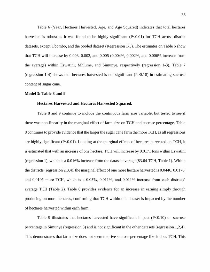
36

Table 6 (Year, Hectares Harvested, Age, and Age Squared) indicates that total hectares

harvested is robust as it was found to be highly significant (P<0.01) for TCH across district

datasets, except Ubombo, and the pooled dataset (Regression 1-3). The estimates on Table 6 show

that TCH will increase by 0.003, 0.002, and 0.005 (0.004%, 0.002%, and 0.006% increase from

the average) within Eswatini, Mhlume, and Simunye, respectively (regression 1-3). Table 7

(regression 1-4) shows that hectares harvested is not significant (P>0.10) in estimating sucrose

content of sugar cane.


Hectares Harvested and Hectares Harvested Squared.

Table 8 and 9 continue to include the continuous farm size variable, but tested to see if

there was non-linearity in the marginal effect of farm size on TCH and sucrose percentage. Table

8 continues to provide evidence that the larger the sugar cane farm the more TCH, as all regressions

are highly significant (P<0.01). Looking at the marginal effects of hectares harvested on TCH, it

is estimated that with an increase of one hectare, TCH will increase by 0.0171 tons within Eswatini

(regression 1), which is a 0.016% increase from the dataset average (83.64 TCH, Table 1). Within

the districts (regression 2,3,4), the marginal effect of one more hectare harvested is 0.0446, 0.0176,

and 0.0105 more TCH, which is a 0.05%, 0.011%, and 0.011% increase from each districts’

average TCH (Table 2). Table 8 provides evidence for an increase in earning simply through

producing on more hectares, confirming that TCH within this dataset is impacted by the number

of hectares harvested within each farm.

Table 9 illustrates that hectares harvested have significant impact (P<0.10) on sucrose

percentage in Simunye (regression 3) and is not significant in the other datasets (regression 1,2,4).

This demonstrates that farm size does not seem to drive sucrose percentage like it does TCH. This

37

could be explained by the fact that sucrose formation is closely associated with genetic potential

and climatic variables, where total yield is also associated with input amounts and timing

(endogenous to the producer) along with genetic potential and climatic variables (exogenous to the

producer).

The adjusted R squared values for the pooled datasets (regression 1) for Model 2 (Table 6)

was 0.085 compared to Model 3 (Table 8) at 0.0912. Adjusted R squared values increased by an

additional 0.15, 0.11, and 0.01 on regressions 2-4 within Table 8 compared to Table 6. Looking at

the Tables 7 and 9 (regressed on sucrose percentage) the differences between adjusted R squared

values are not as large as with the TCH regressions, but this is not surprising as hectares harvested

is not significant within Table 7 and is only significant within one regression (3) in Table 9. Table

7 and 9 (regression 1) report adjusted R squares of 0.076. Adjusted R squared values are higher

within Table 9 (regression 3 and 4), with an additional 0.005 in Simunye, and 0.002 in Ubombo.


Farmer Identifier.

Model 4 (Tables 10 and 11) examines the influence of individual farm management

practices on TCH and sucrose percentage by dummying out each individual sugar cane producer

across growing seasons (denoted by Farmer ID). There were 317 growers included from Mhlume,

30 from Simunye, and 107 from Ubombo, for a total of 454 total Eswatini sugar cane growers.

Appendix 1 and 2 demonstrate that 190 and 165 (Table 10b and Table 11b), out of the 454

producers, were found to be statistically significant (P<0.10, 0.05, 0.01), indicating that TCH and

sucrose percentage varied greatly across producers. This could be due to a number of factors, such

as the impact of HIV/AIDs on the household’s labor capabilities, inequality of training, and lack

of access to production resources, education, etc.

38

In addition, the relatively high adjusted R squared values confirm the robustness of this

factor. Table 11 (regression 1) adjusted R squared values increase between Models 3 and 4 as well,

with Table 11 showing 0.231 compared to Table 9 at 0.076. Throughout Regressions 2-4, all of

Table 10 adjusted R squared values increased by at least 35% from Table 8, and Table 11 increased

by at least 74% from Table 9. The high adjusted R squared values and significant individual

coefficients of the unique farmer identifiers demonstrate that the influence of individual farmer’s

skills, training, and management practices upon sugar cane production is significant. This is could

be encouraging news to the sugar cane industry and the Eswatini Government as training and

access to inputs could help mitigate the differences in yields between producers, regardless of farm

size. Again, this could be reassuring as these models have shown if a producer did well last year

they are likely to do well this year. As such, if highly motivated producers can receive extension

training and obtain access to inputs consistently then there is hope that inertia will prevail, and

they can do well into perpetuity. Differences between producers are likely a function of access to

inputs, which was not available in this study, and warrants further research.


Previous Years’ Performance.

While dummying out each producer increases the model’s predictability it leaves little

room for policy implications and suggestions moving forward. The producer dummy does not

allow for the inclusion of location or farm size, due to the possibility of perfect identification,

which are two important policy attributes for the sugar cane industry and the Eswatini government

in general. The government and Eswatini sugar industry need to know if there are spatial (district)

and size (farm size) components to profitability. Model 5 (Table 12 and 13) attempts to gain the

explanatory power of dummying out each producer but also include the spatial and size

39

components which are crucial for policy. As such, each individual producers’ previous years’ TCH

and sucrose percentage are included as an explanatory variable in place of an individual dummy

for each producer. The variables, year, cane age, and age squared stay within the model.

Previous Years’ Production.

Previous years’ sucrose percentage and TCH, was used in place of the individual farmer’s

ID to provide a more concise measurement for the widespread production variability between

growers attributed to farm specific production practices within Table 12 and 13. For TCH the

previous years’ harvest is significant (P<0.10) in all districts (regression 1-4) for estimating the

current year’s harvest. Table 12 coefficients estimate that previous years’ TCH increases the

present years’ TCH by 0.55 and 0.51 tons within the pooled dataset and Mhlume (regression 1,2)

and 0.70 and 0.79 tons within Simunye and Ubombo (regression 3,4). Table 13 illustrates

significance (P<0.10) significant relationship for estimating sucrose percentage this year based

upon the prior year across Regressions 1,2, and 4, with the only exception being Simunye

(Regression 3). Thus, the results on Table 12 and 13 are preferred to those on Tables 10 and 11

because they eliminate the need for individual producer dummies but still provide a similar amount

of information and allow for policy decisions based on farm size and location to be elicited.


Climatic Effects.

Throughout Tables 4 through 12 the fixed effect of each year was used to proxy for

potential of a climatic influence on TCH and sucrose variations. Tables 4, 6, 8, 10, and 12

(Regression 1) demonstrate that out of the ten years at least six have significant differences on

TCH between years in each model. Tables 5,7,9, and 11 (Regression 1) present at least seven out

of ten years of significant differences on sucrose percentage in each model. To more clearly

40

represent the effects of climatic on sugar cane production, weather data was analyzed and included

in Table 14 and 15.

For increased precision, critical weather thresholds, as defined by the sugar cane

physiology literature, are used within Table 14 and 15 to estimate the effect of climate interactions

with sugar cane production which replaces the year proxy. The sugar cane literature states that

temperatures above 35℃ are destructive to biomass growth in season 1 (the vegetative stage)

(Ebrahim, Zingsheim, El-Shourbagy, Moore, & Komor, 1998; Moore & Botha, 2013).

Time above 35℃ is the calculation of the number of growing degree days at or above this

critical threshold. Table 14 shows indicates the negative and statistically significant (P<0.01)

impact of temperatures above 35℃ in Eswatini (Regression 1) and in the subset of data, Mhlume

(Regression 2). Within Eswatini it is estimated that TCH will decrease by 2.140 tons with an

additional degree day above 35℃, which is equivalent to a 2.5% yield loss from the average TCH

(83.64) for the pooled datset. Mhlume, the largest district by number of sugar cane growers (320,

Appendix 1), expects to lose 2.997 TCH from the one additional degree day above the critical

threshold temperature in Eswatini, a 3.5% decrease from the average Eswatini TCH (83.64) and a

3.7% decrease from the Mhlume average TCH (80.39). Within the other two districts, Simunye

and Ubombo, Time above 35℃ is not a significant indicator for TCH estimates (Table 14).

Figure 15 illustrates that in 2010, Mhlume, Simunye, and Ubombo were exposed to at least

19% more than the dataset average, 4.07 degree days above 35℃, at 4.83, 5.6, and 6.75 days above

35℃. In the most recent weather data year, 2015-2016, Figure 15 demonstrates 8.35, 9.05, and

9.82 degree days above 35℃, which is a 105%, 122%, and 141% increase from the average degree

days for the dataset (4.07 days).

41

To account for the fact that the literature on sugar cane physiology shows that in the second

stage of sugar cane production (sucrose forming stage) that cold temperatures are desirable (as

long they are above freezing) the model includes the effect of the minimum daily temperature on

sucrose percentage.2 Further, the literature shows that rain prior to harvest (in the sucrose formation

stage) can reduce sucrose percentage by promoting new vegetative growth, thus syphoning energy

away from sucrose formation, as well as simply diluting the sucrose percentage. As such, rainfall

in the sucrose formation stage was used as an explanatory variable for sucrose percentage at

harvest.

Within Regression 2-5, it was found that the average minimum temperature does not have

a statistically significant effect on sucrose content in Table 15. In contrast, Regression 1 found

average minimum temperature has significant in estimating sucrose content by eliminating the

district dummy variables (Table 15). This may be due to the location variables perfectly identifying

weather effects and thus shifting the significance from the average minimum temperature variable

to the dummy variables.

Precipitation is highly significant (P<0.01) for sucrose accumulation in Eswatini

(Regression 1) and Mhlume (Regression 2) within Table 15. It is estimated that a one-millimeter

change of precipitation will decrease sucrose percentage by 0.01% in both Mhlume and Eswatini.

Tables 14 and 15 are ultimately the preferred models in the study. These variables are robust and

include climatic data which increases the explanatory power of the models.

2 There were no recorded lows below 0℃ so in this model the colder, the better with respect to

sucrose percentage.

42

Marginal Effect of Hectares Harvested on Production and Revenue.

Using the regression output from Table 8, Figure 16 demonstrates the marginal effect of

hectares harvested on TCH when calculated using Equation 2a3. The marginal effect of TCH is

calculated by using the coefficient estimates from Model 3 (Table 8, Regression 1) for hectares

and hectares squared, with the hectares harvested value (as denoted by 𝐻) varying between 0-

11,500 hectares (by 100 hectares). The largest farm size within this dataset was a farm of 11,555

hectares, hence allowing for Figure 16 to graph all sizes of farms within this dataset. The

estimated change in TCH is added onto the dataset mean Eswatini TCH estimated from Table 8

(Model 3, Regression 1) at 90.52 TCH to graph the Mean TCH on Figure 16. To calculate

revenue per hectare (Equation 3), the average sucrose price of 2,569 emalangeni is used and is

calculated as the average of sucrose price in Eswatini between 2008-2015.4 The new calculated

mean TCH and sucrose percentage being held constant at 0.140 (the estimated average sucrose

percentage from Table 9, Model 3) is used to calculate and graphically represent revenue on

Figure 16.

Figure 16 illustrates the marginal effect of farm size on revenue per hectare. The average

Eswatini sugar cane producer within this dataset harvests 105 hectares (Table 1), which,

according to Figure 16, would be associated with a revenue of 32,858 emalangeni at harvest.

Marginal effects remain positive for more hectares until 5,400 hectares harvested (Figure 16).

For a comparative sense, the revenue earned from sugar cane production is compared with the

Eswatini GDP per capita, which was estimated at 38,888 emalangeni in 2015 (World Bank

3 Note: Figure 17. Marginal Effect of Hectares Harvested on Sucrose Percentage included within

Figures Section for reference only. 4 Sucrose in this sense is not sucrose percentage, but rather total sucrose harvested. Thus, it is

calculated by multiplying TCH by sucrose percentage.

43

Development Indicators Database, 2017). From this per capita GDP estimate, Figure 16

calculations estimate that marginal effects would become negative at 5,500 hectares allowing

that more hectares would not be beneficial above this size and thus an Eswatini sugar cane

grower would be hard pressed to earn even the average per capita GDP as a standard of living.

These estimates are obviously underestimated as this calculation is based only on revenue

and does not include cost of production. Thus, the arbitrary value of 50 hectares for a “small” farm

may be too small to achieve the average standard of living in Eswatini. The marginal effect of

hectares harvested demonstrated in Figure 16 confirm the reality that the smaller farmers in

Eswatini appear to have lower TCH than larger farmers. This could be attributed to the fact the

larger famers have more access to credit and thus can afford optimal amounts and timing of inputs

(which was not modeled here). Larger farmers also have better access to crop dusters to apply

growth inhibitors which can increase TCH. Overall, from a TCH standpoint, larger farms appear

to have higher TCH. Regardless of the cause Table 8 and 9 and Figures 16 indicate that “small”

producers in Eswatini need to be given more attention by the government, the extension service

and NGO’s if the goal is to lift the agricultural community in Eswatini out of poverty.

Marginal Effect of Cane Age on Production and Revenue.

Figure 18 demonstrates the marginal effect of cane age (in months) on TCH and sucrose

percentage when calculated using Equation 1. To calculate the marginal effects on TCH,

coefficient estimates from the preferred Model 6 (Table 14) for Age and Age squared are used

within Equation 1, with the cane age (denoted as 𝐴 in Equation 1a) being changed from 0-20. The

resulting marginal effect of age on TCH from Equation 1a is added onto the mean Eswatini TCH

estimate from Table 14 (Model 6, regression 1), of 81.39 TCH for age of sugar cane (0-20 months)

to calculate the Mean TCH graphed on Figure 18. To calculate the revenue effects of age (Equation

44

3), the average sucrose price, 2,569 emalangeni is used and is calculated as the average of sucrose

price for years 2008-2015 (T. Dlamini, personal correspondence, April 9, 2018). Figure 18 uses

the mean TCH estimate (based on the effects of increasing cane age) and sucrose percentage held

constant at 0.140 (estimated Eswatini sucrose percentage from Table 15, Model 6, regression 1) to

calculate and graph the revenue curve.

Figure 19 illustrates how increasing the cane age will impact sucrose percentage when the

marginal effect is calculated (equation 1b). To calculate the marginal effects on sucrose

percentage, coefficient estimates from Model 6 (Table 14) for Age and Age squared are used

within Equation 1b, with the cane age (denoted as 𝐴 in Equation 1b) being changed from 0-20.

The resulting marginal effect of age on sucrose percentage from Equation 1b is added onto the

mean Eswatini sucrose percentage estimate from Table 14 (Model 6, regression 1), 14.07%, to

calculate the Mean sucrose percentage graphed on Figure 19. Revenue (Equation 3) is calculated

with a constant TCH at 81.39 (Model 6, Table 14), the average sucrose price of 2,569 emalangeni,

and the new calculated Mean sucrose percentages for each age of cane (Figure 19).

Figure 18 and 19 shows the marginal increase of age and allows for the optimal age of

sugar cane for TCH and sucrose percentage to be estimated. According to the age and age squared

coefficients derived from Table 14 and 15, TCH is estimated to have positive marginal effects until

12.72 months, and after this threshold, older cane age becomes a negative impact on TCH. At the

optimal age, 12.72 months old, TCH is estimated at 95.28 TCH and a revenue of 34,458

emalangeni as illustrated on Figure 18. The estimated optimal age of 12.72 slightly higher, but still

representative of the Eswatini actual dataset average cane age, 12.17 months (Table 1).

Sucrose percentage has positive marginal effects until 15.36 months of age, with more

months of age having a negative impact on sucrose content within cane after this threshold. At

45

15.36 months the sucrose percentage is estimated at 14.28% with a revenue of 29,877 emalangeni

(Figure 19). Within the dataset from Eswatini producers, the average sucrose percentage is 14.18%

for Eswatini with the maximum sucrose percentage reaching 17.47% sucrose content (Table 1).

Traditionally, Eswatini sugar cane producer’s aim to harvest their cane within 12 months, but the

harvest age varies based upon climatic variables, mill processing schedule, and producer ability

(N. Dlamini, personal communication, June 12, 2017). The main takeaway from graphing sucrose

percentage by age is to understand that these models demonstrate the non-linearity character of

age and that there is an optimal harvesting period estimated around 12-15 months of age. Out of

the total 4,178 observations in the dataset, 952 observations were harvested between the average

cane age of 12.72 and 15.36 months.

Climatic Scenarios

Using the preferred model (6) within Table 14 and 15 (Regressions 1) the impact of various

future climatic scenarios on sugarcane producer revenue is calculated. By creating a range of

possible climate change scenarios, the goal was to estimate the extent of impact on revenue from

both increases and decreases in precipitation and temperature. A new, hypothetical weather dataset

was created by adding (and subtracting) 0.5 and 1 degree ℃ to all temperature values within the

actual weather data (2008-2016) and then re-calculating the degree day summations over the 35℃

threshold and the new average daily minimum temperatures. To calculate precipitation changes,

actual rainfall data from 2008-2016 was altered by increasing and decreasing precipitation by

2.5%, 5.0%, and 10.0%, respectively.

Within Table 16, the combination of temperature and precipitation effects on revenue,

through changes in TCH and sucrose percentage, was calculated simultaneously. The original

estimated revenue (derived from Model 6, regression 1) was 29,550 emalangeni based on the

46

average sucrose price of 2,569 E/Ha with 11.50 tons per hectare sucrose produced (TCH: 81.4,

Sucrose Percentage: 14.12,). The revenue changes within Table 16 were calculated by adding the

absolute change of TCH and sucrose percentage after exposing them to the aforementioned climate

changes, to the estimated TCH and sucrose percentage values from Table 14 and 15 (regression 1)

to calculate the sucrose produced, which is multiplied by the price to get revenue.

The change in TCH caused by warmer and colder temperature was calculated by taking the

difference between the estimated mean TCH 81.395 based on Model 6 (Table 14, Regression 1

estimates) and the calculated estimated mean TCH when using the mean value of degree days

above 35℃ in each of the hypothetical temperature change scenarios. The changes in sucrose

percentage caused by the increased or decreased temperatures was a function of two climatic

variables, precipitation and average minimum temperature. Sucrose percentage changes caused

only by the average minimum temperature was calculated by taking the difference between the

estimated mean sucrose percentage, 14.07, from Model 6 (Table 15, Regression 1) and the

calculated estimated mean sucrose percentage when using the mean value of average minimum

temperatures during the sucrose phase of the sugar cane lifecycle for hypothetical temperature

change scenario (when no change occurs in precipitation). Sucrose percentage changes caused

only by precipitation was estimated by taking the difference between the mean sucrose percentage

(14.07, estimated from Model 6, Table 15, Regression 1) and the new sucrose percentage when

using the precipitation mean values calculated at increased or decreased levels (from the actual

weather dataset mean precipitation, 649.25 mm), while keeping the average minimum temperature

in season 2 constant at the actual weather dataset mean of 20.90℃. Sucrose percentage effects

from both changes in precipitation and temperature were calculated by taking the difference of the

mean sucrose percentage (14.07, estimated from Model 6, Table 15, Regression 1) and the mean

47

sucrose percentage when re-calculated using the mean precipitation value at each scenarios of

increases or decreases in precipitation (-10%,-5%,-2.5%, 2.5%,5%, and 10%), while keeping the

average minimum temperature values (19.90, 20.40, 21.40, and 21.90 at -1℃, -1/2℃, +1/2℃,

and +1℃, respectively) constant at the means when there is only warming scenarios and no change

in precipitation.

Both increases and decreases in these factors are pertinent because temperature and

precipitation effect biomass growth and sucrose accumulation differently in the two (vegetative

and sucrose formation) cane development stages. As critical cane growth occurs during season

one, the cane is sensitive to increased temperature changes. Precipitation specifically effects the

quality of sucrose content within the second season, with excess rainfall causing low sucrose

content (Gowing, 1977, as cited in, Blackburn, 1984).

Table 16 demonstrates that the temperature effects dominate the precipitation effects with

respect to revenue. For example, within the first column (-1℃) when precipitation is 10% below

the current state, revenue is expected to increase by 1,108 emalangeni per hectare, while a 10%

increase in precipitation portrays a small increase of revenue by 831 emalangeni per hectare as

well. The linear expectation of a 10% increase in precipitation would be -1,108 emalangeni, the

mirror image of the opposite scenario. Instead, the temperature change (in this case cooler)

dominates and allows for the combined positive influence on revenue of 831, even with

precipitation increased at 10%.

The trend for all scenarios demonstrates lower revenues with higher temperatures and more

precipitation. Increased precipitation lends itself to water down the sucrose content. Drought, to

some extent, can be mitigated through the irrigation of sugar cane at pivotal points in the plants

life-cycle and therefore is outweighed by the negative impact of increased temperature in this

48

example. With temperature held constant, less precipitation in season 2 always increases sucrose

percentage, and the reverse is true with more precipitation always decreasing sucrose percentage.5

This reflects through to grower revenue per hectare on Table 16 within row 1 (-10% precipitation)

which is always a higher value than the seventh row, except for when there are no temperature

changes (+10% precipitation). Biologically, this pattern makes sense because too much rain within

season 2 can dilute the sucrose content, causing a lower sucrose percentage upon harvest, which

decreases revenue for the grower. At best, Figure 16 and 17 illustrate that with increased

precipitation (10%) the revenue per hectare increases from the average (29,550.42 E/Hectare) by

2.81% (831 E/Hectare change) and at worst decreases by 4.98% (1,471 E/Hectare loss).

TCH is negatively impacted by the warmer temperature scenarios which cause more degree

days above the critical threshold 35℃. All cases of warmer temperature, as well as those with no

changes in temperature and increased precipitation, cause negative revenue effects (Table 16).

Global temperatures are increasing, and even a 1/2℃ increase in this estimate can cause losses

from 463-731 E/Ha which is a 1.57%-2.48% decrease from the average revenue (29550.42

E/Hectare) (Table 16 and 17).

Table 16 illustrates that if temperatures were to decrease by 1/2 ℃, revenue per hectare

change would be positive between 471-539 emalangeni per hectare revenue when precipitation

stays within 2.5% (more and less) of the present situation which is 1.59-1.83% less than the

average revenue (29550.42 E/Hectare) (Table 17). In comparison, the revenue losses are greater

when increasing 1/2℃ at the same rainfall (+/- 2.5%), with 564-631 E/Ha of losses (11.91-2.14%

decrease from the average, Table 17) estimated emalangeni per hectare on Table 16. In the case of

5 All sugar cane in Eswatini is irrigated and the assumption is irrigation water will be available

when needed.

49

extreme heat increases (+1℃), it can be expected that an average Eswatini grower will lose up to

1,471 emalangeni per hectare, a 4.98% decrease from the average expected revenue, when the

precipitation increases by 10% (Table 17). In the opposite case, revenue was found to increase by

3.75% from the average by earning 1,108 emalangeni per hectare when temperature decreases by

1℃ and precipitation decreases 10%. From these estimates, it is expected that wetter and warmer

climates have negative impacts of losses up to 1,471 E/ha for Eswatini growers. These various

climate change scenarios help demonstrate how the livelihoods of sugarcane farmers in Eswatini

are influenced with even slight changes to rainfall and temperature.

Conclusion

In conclusion, the relationship between farm size and production capabilities was

evidenced and explored through several avenues. First, the SSA classification system found

significant differences between “small” and “large” farm TCH means (Table 4). Looking at the

number of hectares on each farm, there are increasing marginal effects on TCH from adding

additional hectares to the farm up to 5,400 hectares (Figure 16). In addition, the individual farmer

management and production practices significantly impact the TCH regardless of farm size in

Eswatini (Table 11).

The effects of three critical weather variables, time above 35℃, average minimum

temperature, and precipitation, within targeted sugar cane growth stages were significant indicators

for both TCH and sucrose percentage. The power of these changing weather patterns indicates

risks for earning reductions in both physiological growth stages. Hypothetical weather scenarios

of changing weather and precipitation demonstrate lower per hectare revenues for sugar cane

growers in the face of hotter, wetter circumstances.

50

Discussion

This study produced several important findings for the sugarcane industry in Eswatini.

First, this study found differences between revenue per hectare for small (less than 50 hectares),

medium (50-1000 hectares) and large (greater than 1000 hectares) sugar cane farms. Small farms

were found to produce less revenue per hectare than medium and large farms. This can be seen as

an opportunity for the Eswatini government, extension services, NGO’s and sugar cane growing

associations to invest in. While input data was not available for this study it can be assumed that

small scale producers likely have less access to timely inputs, than those with larger farms. This

study’s results may also be a manifestation of the effects of HIV/AIDS as output from small farms

is more likely to be affected from HIV/AIDS than large farms as small farms rely on family and

not hired labor. Extension training and support could be targeted towards smaller farms to increase

their productivity per hectare.

A better understanding for production issues, and those specifically affecting smallholder

growers, could be gathered through more specific information regarding individual’s farming

practices. For example, data such as the number and type of workers on the farm, planting and

harvesting dates would provide researchers the ability to narrow in on labor, cane age, and mill

timing effects. Within this study, the assumption was that all sugar cane was irrigated, and this

might not be the case according to the significance of weather elements specifically in Mhlume.

Additional information in regard to the irrigation systems and usage on individual farms could also

shed light on the potential disadvantage of smallholder farmers for on-demand irrigation due to

lack of payment for water and water rights, poor management planning, and governance issues.

This input data could also help the government narrow in on what type of training and education

would be most effective for increased production for growers.

51

Second, a large portion of yield variability across the sugar industry is a function of the

producer him/herself. The largest explanatory variable for yield was using fixed effects to delineate

producers across time. This should be viewed with optimism for the sugar cane industry as it

appears that while climate and other exogenous variables contribute to total yield that the

producers themselves are the greatest drivers. Thus again, if the Eswatini government, extension

services, NGO’s and sugar cane growing associations could invest in training, it could be possible

to lower the gap between those farmers who have the highest revenue per hectare and those who

have low revenue per hectare. While there are inherent work differences between everyone, it is a

safe assumption that those who are well below the average yield (and thus more likely to be food

insecure) would have as great as an incentive to work just as hard as someone who has above

average yields. If this assumption holds true, then a large-scale extension campaign on best

management practices could lift those producers with low yields closer to the median. Assuming

that people want to better their livelihoods and are willing to work to accomplish this goal this

study’s finding that producers themselves and not exogenous factors drive revenue can be seen as

an opportunity for education in best management practices.

Given the recent El Nino drought and extreme heat events this study also set out to model

the effects climate on sugarcane production in Eswatini. Given the sensitivity of sugarcane to

extreme heat events, above 35℃, in the vegetative stage and increases in average daily minimum

temperatures in the sucrose filling stage this study found that small changes (0.5℃) in average

daily temperatures from the observed actual temperatures result in large negative revenue

implications for sugarcane producers. Changes in temperature were shown to have higher impact

on revenue than changes in precipitation across all scenarios. From these results, investments in

heat tolerant breeding in sugarcane cultivars may be warranted in the face of a warming world.

52

This study was the nexus of endogenous and exogenous factors affecting sugarcane

production in Eswatini. Optimistically, this study found that the majority of variation in sugarcane

revenue is determined by endogenous factors, producers themselves. As such, investment in

training and best management practices may help to lift marginalized populations out of poverty.

It also appears that a warming environment will have significant effects on the livelihoods of sugar

cane producers. These results should be a call to international sugarcane community for increased

research and development in heat tolerant sugarcane cultivars.

This research is only one part of a larger effort to develop sustainable sugarcane production

in Eswatini. Achieving this goal in the face of climate change requires an integrated approach

across economic, agronomic, hydrologic, and other scientific disciplines whose research can be

guided by the results provided in this study. Continued observation of the interaction between

increasingly variable weather conditions and sugarcane production outcomes will allow

refinement and enhancement of this study and provide plant breeders, agricultural policy makers

in Eswatini, and private sugar enterprises with important direction for sustaining production and

enhancing livelihoods of the poorest of the poor in an increasingly hot future.

53

Tables6

Table 1. Descriptive Statistics (n=4178)

Variable Mean Standard

Deviation

Median Min Max

Hectares

Harvested 105.18 726.59 5.67 1.468 11,555.22

Total Tons

Cane 10716.49 75948.71 443.09 13.46 1406341

Total Sucrose 1521.6 10849.17 64.37 2.01 205780.2

Sucrose

Percentage 14.18 1.08 14.23 1.09 17.47

Average Age 12.17 1.99 11.99 1.54 50.97

Tons of Cane

per Hectares

Harvested

83.64 29.94 85.94 2.57 479.08

TSH 11.88 4.39 12.17 0.38 70.54

6 Within all tables, Marginal Effect of Age and Hectares Harvested reported as:

Marginal effect of Age = 𝛽4 + 2𝛽5𝐴 + 𝛽5, with 𝐴: Average Age of 12.2 months and

Marginal effect of Hectares = 𝛽6 + 2𝛽7𝐻 + 𝛽7, with H: Average hectares harvested of 105

hectares.

54

Table 2. Mhlume Descriptive Statistics (n=3072)


Deviation Median Min Max

Hectares

Harvested 43.78 390.95 4.20 1.83 7785.08

Total Tons

Cane 4279.09 38152.75 337.23 13.46 791666.02

Total Sucrose 621.54 5582.19 48.45 2.01 109748.31

Sucrose

Percentage 14.29 1.15 14.42 8.22 17.47

Average Age 12.06 1.67 11.96 1.54 34.70

Tons of Cane

per Hectares

Harvested

80.39 30.61 82.19 2.57 479.08

Tons of Sugar

per Hectare 11.55 4.57 11.82 0.38 70.54

Simunye Descriptive Statistics (n=253)



Hectares

Harvested 609.00 2101.72 71.80 4.78 11555.22

Total Tons

Cane 65835.00 229512.33 5967.74 242.02 1406341.34

Total Sucrose 9422.62 32923.41 825.12 36.19 205780.18

Sucrose

Percentage 14.01 1.01 14.08 8.22 15.76

Average Age 12.30 2.21 12.10 9.37 39.59

Tons of Cane

per Hectares

Harvested

94.13 23.39 96.17 32.15 167.19

Tons of Sugar

per Hectare 13.18 3.35 13.54 0.91 23.14

Ubombo Descriptive Statistics (n=853)



Hectares

Harvested 176.90 797.92 30.20 1.47 8836.13

Total Tons

Cane 17552.04 79710.72 2463.68 110.10 812845.78

Total Sucrose 2419.65 11039.37 338.85 16.39 113935.13

Sucrose

Percentage 13.83 0.71 13.87 10.90 15.80

Average Age 12.54 2.79 12.17 4.04 50.97

Tons of Cane

per Hectares

Harvested

92.23 26.69 92.21 19.95 354.11

Tons of Sugar

per Hectare 12.70 3.75 12.69 2.62 46.80

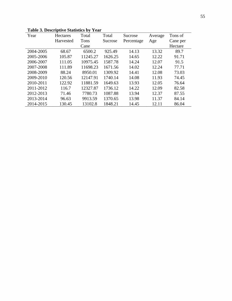
55

Table 3. Descriptive Statistics by Year

Year Hectares

Harvested

Total

Tons

Cane

Total

Sucrose

Sucrose

Percentage

Average

Age

Tons of

Cane per

Hectare

2004-2005 68.67 6500.2 925.49 14.13 13.32 89.7

2005-2006 105.87 11245.27 1626.25 14.65 12.22 91.71

2006-2007 111.05 10975.45 1587.78 14.24 12.07 91.5

2007-2008 111.89 11698.23 1671.56 14.02 12.24 77.71

2008-2009 88.24 8950.01 1309.92 14.41 12.08 73.03

2009-2010 120.56 12147.91 1740.14 14.08 11.93 74.45

2010-2011 122.92 11881.59 1649.63 13.93 12.05 76.64

2011-2012 116.7 12327.87 1736.12 14.22 12.09 82.58

2012-2013 71.46 7780.73 1087.88 13.94 12.37 87.55

2013-2014 96.63 9913.59 1370.65 13.98 11.37 84.14

2014-2015 130.45 13102.8 1848.21 14.45 12.11 86.04

56

Table 4. Model 1a Dependent variable: TCH

Eswatini Mhlume Simunye Ubombo (1) (2) (3) (4)

Simunye 8.137***

(1.982)

Ubombo 10.448***

(1.138)

2005-2006 0.094 1.094 1.471 -5.428 (2.040) (2.353) (6.908) (4.795)

2006-2007 -0.375 1.381 -10.893 -5.062 (2.047) (2.364) (6.873) (4.792)

2007-2008 -14.037*** -19.844*** 3.062 -1.150 (2.064) (2.389) (7.181) (4.947)

2008-2009 -18.709*** -19.846*** -14.974** -16.970*** (2.438) (2.893) (6.739) (5.706)

2009-2010 -17.881*** -20.193*** -16.202** -13.857*** (2.085) (2.419) (6.959) (4.757)

2010-2011 -15.456*** -14.325*** -16.136** -18.687*** (2.081) (2.404) (7.394) (5.260)

2011-2012 -9.560*** -8.721*** -12.356* -14.244*** (2.057) (2.388) (6.814) (4.682)

2012-2013 -3.238 0.364 -13.936** -17.467*** (2.091) (2.383) (6.842) (5.256)

2013-2014 -7.385*** -6.047** -10.993 -15.976*** (2.154) (2.422) (6.879) (5.749)

2014-2015 -5.659*** -3.310 -7.204 -15.141*** (2.094) (2.399) (6.953) (5.029)

Hectare Class: Medium -12.956*** -7.321 -26.624*** -12.669** (3.511) (7.004) (4.788) (4.999)

Hectare Class: Small -23.264*** -28.225*** -20.649*** -12.556*** (3.414) (6.792) (4.868) (4.797)

Age -0.952 2.276* 2.920 0.391 (0.598) (1.210) (2.558) (1.100)

Age Squared 0.005 -0.142*** -0.063 -0.014

(0.016) (0.044) (0.057) (0.023)

Marginal Effect of Age -0.83 -1.1780 1.3802 0.0506

Constant 121.197*** 107.682*** 98.965*** 112.600*** (6.381) (11.003) (24.202) (13.275)

Observations 4,178 3,072 253 853

R2 0.104 0.124 0.190 0.068

Adjusted R2 0.101 0.120 0.143 0.053

Residual Std. Error 28.392 (df = 4161) 28.711 (df = 3057) 21.660 (df = 238) 25.981 (df = 838)

F Statistic 30.334*** (df = 16; 4161) 30.968*** (df = 14; 3057) 3.996*** (df = 14; 238) 4.372*** (df = 14; 838)

Note: *p<0.1; **p<0.05; ***p<0.01

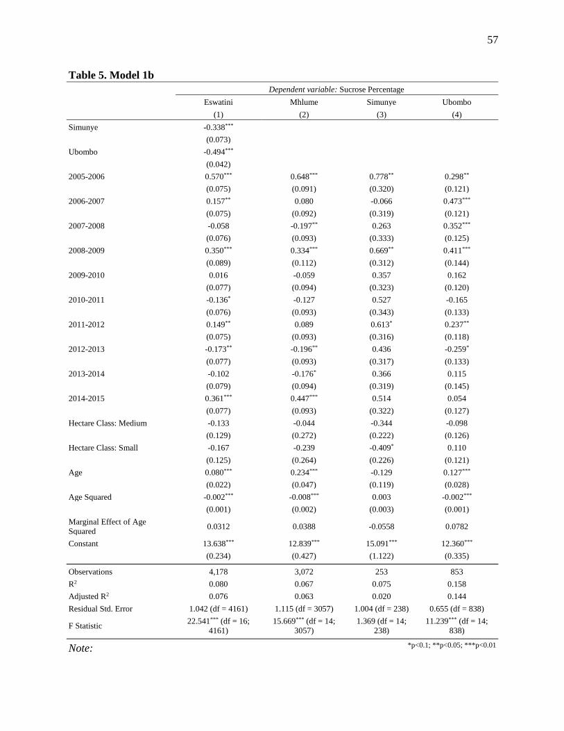
57

Table 5. Model 1b Dependent variable: Sucrose Percentage


Simunye -0.338***

(0.073)

Ubombo -0.494***

(0.042)

2005-2006 0.570*** 0.648*** 0.778** 0.298** (0.075) (0.091) (0.320) (0.121)

2006-2007 0.157** 0.080 -0.066 0.473*** (0.075) (0.092) (0.319) (0.121)

2007-2008 -0.058 -0.197** 0.263 0.352*** (0.076) (0.093) (0.333) (0.125)

2008-2009 0.350*** 0.334*** 0.669** 0.411*** (0.089) (0.112) (0.312) (0.144)

2009-2010 0.016 -0.059 0.357 0.162 (0.077) (0.094) (0.323) (0.120)

2010-2011 -0.136* -0.127 0.527 -0.165 (0.076) (0.093) (0.343) (0.133)

2011-2012 0.149** 0.089 0.613* 0.237** (0.075) (0.093) (0.316) (0.118)

2012-2013 -0.173** -0.196** 0.436 -0.259* (0.077) (0.093) (0.317) (0.133)

2013-2014 -0.102 -0.176* 0.366 0.115 (0.079) (0.094) (0.319) (0.145)

2014-2015 0.361*** 0.447*** 0.514 0.054 (0.077) (0.093) (0.322) (0.127)

Hectare Class: Medium -0.133 -0.044 -0.344 -0.098 (0.129) (0.272) (0.222) (0.126)

Hectare Class: Small -0.167 -0.239 -0.409* 0.110 (0.125) (0.264) (0.226) (0.121)

Age 0.080*** 0.234*** -0.129 0.127*** (0.022) (0.047) (0.119) (0.028)

Age Squared -0.002*** -0.008*** 0.003 -0.002***

(0.001) (0.002) (0.003) (0.001)

Marginal Effect of Age

Squared 0.0312 0.0388 -0.0558 0.0782

Constant 13.638*** 12.839*** 15.091*** 12.360*** (0.234) (0.427) (1.122) (0.335)

Observations 4,178 3,072 253 853

R2 0.080 0.067 0.075 0.158

Adjusted R2 0.076 0.063 0.020 0.144


F Statistic 22.541*** (df = 16;

4161)

15.669*** (df = 14;

3057)

1.369 (df = 14;

238)

11.239*** (df = 14;

838)

Note: *p<0.1; **p<0.05; ***p<0.01

58

Table 6. Model 2a

Dependent variable: TCH


Simunye 13.143***

(1.912)

Ubombo 12.554***

(1.121)

2005-2006 0.256 1.578 2.472 -5.588 (2.058) (2.399) (7.203) (4.805)

2006-2007 -0.180 1.865 -9.333 -5.219 (2.065) (2.411) (7.158) (4.802)

2007-2008 -13.879*** -19.225*** 5.558 -1.303 (2.082) (2.436) (7.469) (4.958)

2008-2009 -19.201*** -20.671*** -12.823* -17.047*** (2.459) (2.950) (7.011) (5.719)

2009-2010 -17.533*** -19.390*** -14.138* -13.894*** (2.104) (2.466) (7.242) (4.768)

2010-2011 -15.180*** -13.350*** -12.661 -18.759*** (2.099) (2.450) (7.670) (5.272)

2011-2012 -9.244*** -7.931*** -11.304 -14.302*** (2.075) (2.434) (7.104) (4.692)

2012-2013 -3.153 1.267 -12.859* -17.627*** (2.110) (2.429) (7.133) (5.265)

2013-2014 -7.234*** -5.233** -10.048 -16.117*** (2.173) (2.469) (7.172) (5.760)

2014-2015 -5.345** -2.486 -6.087 -15.192*** (2.113) (2.446) (7.249) (5.039)

Hectares Harvested 0.003*** 0.005*** 0.002*** 0.002 (0.001) (0.001) (0.001) (0.001)

Age -0.878 2.438** 2.912 0.389 (0.603) (1.234) (2.668) (1.103)

Age Squared 0.001 -0.153*** -0.061 -0.014

(0.016) (0.045) (0.059) (0.023)


Squared -0.8536 -1.2952 1.4236 0.0474

Constant 98.287*** 80.225*** 74.373*** 100.315*** (5.419) (8.722) (24.866) (12.610)

Observations 4,178 3,072 253 853

R2 0.088 0.089 0.116 0.063

Adjusted R2 0.085 0.085 0.068 0.049


F Statistic 26.803*** (df = 15;

4162)

22.898*** (df = 13;

3058)

2.403*** (df = 13;

239) 4.346*** (df = 13; 839)

Note: *p<0.1; **p<0.05; ***p<0.01

59

Table 7. Model 2b

Dependent variable: Sucrose Percentage


Simunye -0.326***

(0.070)

Ubombo -0.488***

(0.041)

2005-2006 0.570*** 0.653*** 0.788** 0.299** (0.075) (0.091) (0.321) (0.122)

2006-2007 0.157** 0.084 -0.045 0.475*** (0.075) (0.092) (0.319) (0.122)

2007-2008 -0.057 -0.192** 0.288 0.357*** (0.076) (0.093) (0.333) (0.126)

2008-2009 0.349*** 0.327*** 0.685** 0.427*** (0.089) (0.112) (0.312) (0.145)

2009-2010 0.018 -0.052 0.382 0.165 (0.076) (0.094) (0.322) (0.121)

2010-2011 -0.135* -0.118 0.550 -0.161 (0.076) (0.093) (0.341) (0.134)

2011-2012 0.149** 0.096 0.622* 0.238** (0.075) (0.093) (0.316) (0.119)

2012-2013 -0.173** -0.188** 0.445 -0.237* (0.077) (0.093) (0.318) (0.134)

2013-2014 -0.102 -0.169* 0.377 0.136 (0.079) (0.094) (0.319) (0.146)

2014-2015 0.362*** 0.454*** 0.524 0.055 (0.077) (0.093) (0.323) (0.128)

Hectares Harvested 0.00003 0.0001 0.00004 -0.00001 (0.00002) (0.0001) (0.00003) (0.00003)

Age 0.081*** 0.235*** -0.128 0.124*** (0.022) (0.047) (0.119) (0.028)

Age Squared -0.002*** -0.008*** 0.003 -0.002***

(0.001) (0.002) (0.003) (0.001)


Squared 0.0322 0.0398 -0.0548 0.0752

Constant 13.472*** 12.609*** 14.719*** 12.432*** (0.197) (0.332) (1.107) (0.320)

Observations 4,178 3,072 253 853

R2 0.080 0.065 0.068 0.142

Adjusted R2 0.076 0.061 0.017 0.129


F Statistic 24.044*** (df = 15;

4162)

16.370*** (df = 13;

3058)

1.331 (df = 13;

239)

10.699*** (df = 13;

839)

Note: *p<0.1; **p<0.05; ***p<0.01

60



Simunye 12.660***

(1.907)

Ubombo 11.703***

(1.128)

2005-2006 0.310 1.383 2.242 -5.424 (2.051) (2.380) (6.981) (4.791)

2006-2007 -0.198 1.617 -10.802 -5.052 (2.058) (2.391) (6.947) (4.788)

2007-2008 -13.912*** -19.507*** 3.207 -1.110 (2.075) (2.416) (7.262) (4.943)

2008-2009 -18.978*** -20.311*** -14.141** -16.691*** (2.451) (2.926) (6.803) (5.703)

2009-2010 -17.636*** -19.741*** -15.961** -13.802*** (2.096) (2.446) (7.034) (4.753)

2010-2011 -15.273*** -13.724*** -14.824** -18.686*** (2.092) (2.430) (7.453) (5.256)

2011-2012 -9.304*** -8.272*** -12.215* -14.244*** (2.068) (2.415) (6.889) (4.678)

2012-2013 -3.091 0.780 -13.753** -17.326*** (2.103) (2.410) (6.916) (5.250)

2013-2014 -7.230*** -5.538** -10.965 -15.890*** (2.166) (2.449) (6.954) (5.743)

2014-2015 -5.452*** -2.911 -6.952 -15.172*** (2.106) (2.426) (7.029) (5.024)

Hectares Harvested 0.014*** 0.046*** 0.018*** 0.011*** (0.002) (0.006) (0.004) (0.004)

Hectares Harvested Squared -0.00000*** -0.00001*** -0.00000*** -0.00000**

(0.00000) (0.00000) (0.00000) (0.00000)

Marginal Effect of Hectares Harvested 0.01370931 0.0445984 0.01760437 0.01051162

Age -0.922 2.255* 3.050 0.375 (0.601) (1.224) (2.586) (1.099)

Age Squared 0.003 -0.145*** -0.063 -0.013

(0.016) (0.045) (0.058) (0.023)


Constant 98.303*** 80.749*** 71.599*** 99.486*** (5.401) (8.649) (24.110) (12.576)

Observations 4,178 3,072 253 853

R2 0.095 0.104 0.173 0.070

Adjusted R2 0.091 0.100 0.124 0.054


F Statistic 27.185*** (df = 16;

4161)

25.385*** (df = 14;

3057)

3.549*** (df = 14;

238)

4.500*** (df = 14;

838)

Note: *p<0.1; **p<0.05; ***p<0.01

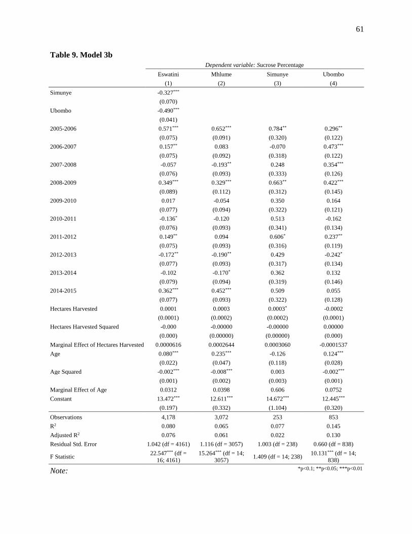
61



Simunye -0.327***

(0.070)

Ubombo -0.490***

(0.041)

2005-2006 0.571*** 0.652*** 0.784** 0.296** (0.075) (0.091) (0.320) (0.122)

2006-2007 0.157** 0.083 -0.070 0.473*** (0.075) (0.092) (0.318) (0.122)

2007-2008 -0.057 -0.193** 0.248 0.354*** (0.076) (0.093) (0.333) (0.126)

2008-2009 0.349*** 0.329*** 0.663** 0.422*** (0.089) (0.112) (0.312) (0.145)

2009-2010 0.017 -0.054 0.350 0.164 (0.077) (0.094) (0.322) (0.121)

2010-2011 -0.136* -0.120 0.513 -0.162 (0.076) (0.093) (0.341) (0.134)

2011-2012 0.149** 0.094 0.606* 0.237** (0.075) (0.093) (0.316) (0.119)

2012-2013 -0.172** -0.190** 0.429 -0.242* (0.077) (0.093) (0.317) (0.134)

2013-2014 -0.102 -0.170* 0.362 0.132 (0.079) (0.094) (0.319) (0.146)

2014-2015 0.362*** 0.452*** 0.509 0.055 (0.077) (0.093) (0.322) (0.128)

Hectares Harvested 0.0001 0.0003 0.0003* -0.0002 (0.0001) (0.0002) (0.0002) (0.0001)

Hectares Harvested Squared -0.000 -0.00000 -0.00000 0.00000

(0.000) (0.00000) (0.00000) (0.000)

Marginal Effect of Hectares Harvested 0.0000616 0.0002644 0.0003060 -0.0001537

Age 0.080*** 0.235*** -0.126 0.124*** (0.022) (0.047) (0.118) (0.028)

Age Squared -0.002*** -0.008*** 0.003 -0.002***

(0.001) (0.002) (0.003) (0.001)

Marginal Effect of Age 0.0312 0.0398 0.606 0.0752

Constant 13.472*** 12.611*** 14.672*** 12.445*** (0.197) (0.332) (1.104) (0.320)

Observations 4,178 3,072 253 853

R2 0.080 0.065 0.077 0.145

Adjusted R2 0.076 0.061 0.022 0.130


F Statistic 22.547*** (df =

16; 4161)

15.264*** (df = 14;

3057) 1.409 (df = 14; 238)

10.131*** (df = 14;

838)

Note: *p<0.1; **p<0.05; ***p<0.01

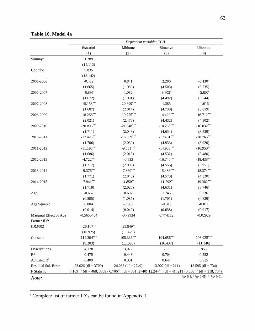
62

Table 10. Model 4a

Dependent variable: TCH


Simunye 1.289

(14.113)

Ubombo 9.835

(13.142)

2005-2006 -0.422 0.841 2.200 -6.130* (1.665) (1.980) (4.503) (3.535)

2006-2007 -0.897 1.082 -9.803** -5.807 (1.672) (1.991) (4.492) (3.544)

2007-2008 -15.153*** -20.699*** 1.385 -1.616 (1.687) (2.014) (4.738) (3.659)

2008-2009 -18.266*** -19.775*** -14.429*** -16.712*** (2.021) (2.473) (4.432) (4.302)

2009-2010 -20.095*** -21.948*** -18.268*** -16.032*** (1.711) (2.043) (4.634) (3.539)

2010-2011 -17.425*** -16.069*** -17.431*** -20.765*** (1.706) (2.030) (4.933) (3.920)

2011-2012 -11.193*** -9.551*** -14.933*** -16.950*** (1.686) (2.015) (4.532) (3.480)

2012-2013 -4.722*** -0.833 -16.746*** -18.438*** (1.717) (2.009) (4.556) (3.951)

2013-2014 -9.376*** -7.360*** -15.486*** -18.374*** (1.771) (2.046) (4.573) (4.320)

2014-2015 -7.941*** -4.850** -11.792** -19.382*** (1.719) (2.025) (4.631) (3.746)

Age -0.667 0.697 1.745 0.236 (0.505) (1.087) (1.701) (0.829)

Age Squared 0.004 -0.061 -0.040 -0.011

(0.014) (0.040) (0.038) (0.017)

Marginal Effect of Age -0.5650484 -0.79934 0.774112 -0.02929

Farmer ID1:

IDM002 -26.107** -25.949**

(10.925) (11.429)

Constant 112.304*** 105.336*** 104.656*** 108.925***

(9.283) (11.395) (16.437) (11.346)

Observations 4,178 3,072 253 853

R2 0.475 0.448 0.704 0.582

Adjusted R2 0.409 0.381 0.647 0.515



Note: *p<0.1; **p<0.05; ***p<0.01

1 Complete list of farmer ID’s can be found in Appendix 1.

63



Simunye -0.762

(0.582)

Ubombo -1.245**

(0.542)

2005-2006 0.582*** 0.670*** 0.847*** 0.355*** (0.069) (0.083) (0.319) (0.116)

2006-2007 0.146** 0.076 -0.014 0.520*** (0.069) (0.083) (0.318) (0.116)

2007-2008 -0.064 -0.202** 0.377 0.443*** (0.070) (0.084) (0.335) (0.120)

2008-2009 0.387*** 0.380*** 0.701** 0.537*** (0.083) (0.103) (0.313) (0.141)

2009-2010 0.004 -0.066 0.416 0.224* (0.071) (0.085) (0.328) (0.116)

2010-2011 -0.159** -0.151* 0.600* -0.071 (0.070) (0.085) (0.349) (0.129)

2011-2012 0.130* 0.073 0.662** 0.291** (0.070) (0.084) (0.321) (0.114)

2012-2013 -0.189*** -0.197** 0.485 -0.203 (0.071) (0.084) (0.322) (0.130)

2013-2014 -0.146** -0.215** 0.410 0.190 (0.073) (0.086) (0.323) (0.142)

2014-2015 0.356*** 0.450*** 0.532 0.120 (0.071) (0.085) (0.328) (0.123)

Age 0.087*** 0.192*** -0.125 0.161*** (0.021) (0.045) (0.120) (0.027)

Age Squared -0.002*** -0.006*** 0.003 -0.003***

(0.001) (0.002) (0.003) (0.001)

Marginal Effect of Age 0.04664446 0.036845 -0.0622546 0.099036

Farmer ID1:

IDM002 -2.350*** -2.349***

(0.451) (0.478)

Constant 14.215*** 13.673*** 14.954*** 12.033*** (0.383) (0.476) (1.163) (0.372)

Observations 4,178 3,072 253 853

R2 0.318 0.317 0.212 0.361

Adjusted R2 0.231 0.235 0.059 0.258


F Statistic 3.688*** (df = 468; 3709) 3.846*** (df = 331; 2740) 1.387* (df = 41; 211) 3.513*** (df = 118; 734)

Note: *p<0.1; **p<0.05; ***p<0.01

1 Complete farmer ID list can be found in Appendix 2.

64



Simunye 6.105***

(1.664)

Ubombo 4.793***

(1.000)

2005-2006 -46.435*** 9.506 -5.378 -123.820*** (10.653) (17.581) (15.103) (12.433)

2006-2007 -45.929*** 10.401 -18.228 -118.558*** (10.641) (17.574) (14.986) (12.347)

2007-2008 -60.222*** -11.683 4.395 -115.714*** (10.643) (17.584) (14.996) (12.382)

2008-2009 -57.319*** -1.491 -21.410 -134.355*** (10.701) (17.642) (14.925) (12.551)

2009-2010 -55.138*** -1.324 -14.321 -125.078*** (10.647) (17.580) (14.963) (12.335)

2010-2011 -51.302*** 4.903 -8.162 -126.421*** (10.648) (17.593) (15.075) (12.428)

2011-2012 -45.385*** 10.381 -9.092 -118.164*** (10.644) (17.577) (14.941) (12.316)

2012-2013 -43.750*** 14.429 -11.677 -125.197*** (10.649) (17.587) (14.938) (12.428)

2013-2014 -51.432*** 3.877 -9.214 -121.472*** (10.655) (17.568) (14.938) (12.526)

2014-2015 -47.816*** 8.856 -6.060 -125.384*** (10.647) (17.581) (14.963) (12.383)

Previous Year's TCH 0.558*** 0.512*** 0.770*** 0.793***

(0.014) (0.016) (0.045) (0.026)

Age -0.395 -0.705** 1.815** -0.087 (0.250) (0.308) (0.869) (0.415)

Age Squared 0.013** 0.027*** 0.022 0.004

(0.005) (0.010) (0.030) (0.005)


Constant 87.563*** 37.719** 5.609 140.196***

(11.106) (17.819) (19.574) (13.921)

Observations 3,721 2,752 223 746

R2 0.370 0.331 0.621 0.611

Adjusted R2 0.367 0.327 0.598 0.604



Note: *p<0.1; **p<0.05; ***p<0.01

65



Simunye -0.209***

(0.072)

Ubombo -0.368***

(0.043)

2005-2006 0.740 0.874 0.603 0.568 (0.463) (0.779) (1.084) (0.463)

2006-2007 0.135 0.102 -0.345 0.660 (0.463) (0.779) (1.077) (0.460)

2007-2008 0.017 -0.012 0.130 0.502 (0.463) (0.779) (1.076) (0.461)

2008-2009 0.519 0.607 0.555 0.557 (0.466) (0.782) (1.072) (0.467)

2009-2010 0.083 0.090 0.216 0.317 (0.463) (0.779) (1.074) (0.459)

2010-2011 -0.023 0.081 0.367 0.039 (0.463) (0.780) (1.080) (0.463)

2011-2012 0.293 0.308 0.460 0.492 (0.463) (0.779) (1.072) (0.459)

2012-2013 -0.073 0.003 0.280 -0.077 (0.463) (0.780) (1.072) (0.463)

2013-2014 0.039 0.044 0.244 0.452 (0.464) (0.779) (1.072) (0.467)

2014-2015 0.532 0.718 0.355 0.282 (0.463) (0.779) (1.073) (0.461)

Previous Year's Sucrose

Percentage

0.261*** 0.286*** 0.057 0.236***

(0.016) (0.019) (0.069) (0.036)

Age 0.029*** 0.009 -0.058 0.093*** (0.011) (0.014) (0.062) (0.016)

Age Squared 0.0002 0.001 0.003 -0.0001

(0.0002) (0.0004) (0.002) (0.0002)

Marginal Effect of Age 0.0347 0.0219 0.0225 0.0914

Constant 9.981*** 9.766*** 13.186*** 9.063*** (0.537) (0.834) (1.637) (0.744)

Observations 3,721 2,752 223 746

R2 0.140 0.134 0.066 0.204

Adjusted R2 0.137 0.130 0.007 0.190


F Statistic 40.341*** (df = 15;

3705)

32.503*** (df = 13;

2738)

1.128 (df = 13;

209)

14.423*** (df = 13;

732)

Note: *p<0.1; **p<0.05; ***p<0.01

66


Pooled

Dataset Eswatini Mhlume Simunye Ubombo

(1) (2) (3) (4) (5)

Simunye 3.226*

(1.894)

Ubombo 3.371***

(1.294)

Hectares Harvested 0.002*** 0.002*** 0.004** 0.001** 0.002 (0.001) (0.001) (0.002) (0.001) (0.001)

Previous Year's TCH 0.456*** 0.445*** 0.446*** 0.473*** 0.395*** (0.016) (0.016) (0.020) (0.055) (0.032)

Age 2.588*** 2.484*** 5.188*** -0.635 1.619 (0.922) (0.922) (1.357) (7.339) (1.247)

Age Squared -0.096*** -0.094*** -0.200*** 0.004 -0.032 (0.029) (0.029) (0.046) (0.256) (0.034)

Marginal Effect of Age 0.2456 0.1924 0.3151 -0.5380 0.8409

Time above 35C in

Season 1 -1.613*** -2.140*** -2.997*** -1.443 -0.435

(0.560) (0.594) (0.816) (1.805) (0.837)

Constant 30.224*** 32.078*** 16.355 55.018 37.352*** (7.350) (7.369) (10.219) (51.932) (11.455)

Observations 2,433 2,433 1,752 180 501

R2 0.267 0.270 0.254 0.335 0.247

Adjusted R2 0.266 0.268 0.252 0.316 0.239

Residual Std. Error 23.505 (df =

2427)

23.474 (df =

2425)

25.079 (df =

1746)

18.766 (df =

174)

18.272 (df =

495)

F Statistic 177.031*** (df

= 5; 2427)

127.966*** (df

= 7; 2425)

119.050***

(df = 5; 1746)

17.539*** (df

= 5; 174)

32.405*** (df

= 5; 495)

Note: *p<0.1; **p<0.05; ***p<0.01

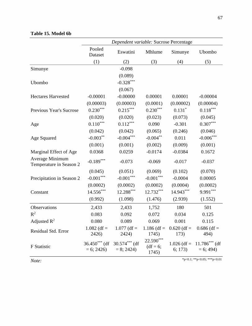
67

Table 15. Model 6b

Dependent variable: Sucrose Percentage

Pooled

Dataset Eswatini Mhlume Simunye Ubombo

(1) (2) (3) (4) (5)

Simunye -0.098

(0.089)

Ubombo -0.328***

(0.067)

Hectares Harvested -0.00001 -0.00000 0.00001 0.00001 -0.00004 (0.00003) (0.00003) (0.0001) (0.00002) (0.00004)

Previous Year's Sucrose 0.230*** 0.215*** 0.230*** 0.131* 0.118*** (0.020) (0.020) (0.023) (0.073) (0.045)

Age 0.110*** 0.112*** 0.090 -0.301 0.307*** (0.042) (0.042) (0.065) (0.246) (0.046)

Age Squared -0.003** -0.004*** -0.004** 0.011 -0.006*** (0.001) (0.001) (0.002) (0.009) (0.001)

Marginal Effect of Age 0.0368 0.0259 -0.0174 -0.0384 0.1672

Average Minimum

Temperature in Season 2 -0.189*** -0.073 -0.069 -0.017 -0.037

(0.045) (0.051) (0.069) (0.102) (0.070)

Precipitation in Season 2 -0.001*** -0.001*** -0.001*** -0.0004 0.00005 (0.0002) (0.0002) (0.0002) (0.0004) (0.0002)

Constant 14.556*** 12.288*** 12.732*** 14.943*** 9.991*** (0.992) (1.098) (1.476) (2.939) (1.552)

Observations 2,433 2,433 1,752 180 501

R2 0.083 0.092 0.072 0.034 0.125

Adjusted R2 0.080 0.089 0.069 0.001 0.115

Residual Std. Error 1.082 (df =

2426)

1.077 (df =

2424)

1.186 (df =

1745)

0.620 (df =

173)

0.686 (df =

494)

F Statistic 36.450*** (df

= 6; 2426)

30.574*** (df

= 8; 2424)

22.590***

(df = 6;

1745)

1.026 (df =

6; 173)

11.786*** (df

= 6; 494)

Note: *p<0.1; **p<0.05; ***p<0.01

68

Table 16. Revenue change per hectare (SZL E) impact from Climate Change Scenarios1

Temperature Changes in Season 1

Precipitation Changes in

Season 2 -1 ℃ -1/2 ℃ No Change

+1/2 ℃

+1 ℃

-10% 1,108.57 642.76 135.82 (463.89) (1,208.69)

-5% 1,039.36 574.15 67.91 (530.88) (1,274.39)

-2.5% 1,004.75 539.84 33.95 (564.37) (1,307.25)

No Change 970.14 505.54 - (597.86) (1,340.10)

+2.5% 935.54 471.23 (33.95) (631.35) (1,372.96)

+5% 900.93 436.93 (67.91) (664.84) (1,405.81)

+10% 831.72 368.31 (135.82) (731.83) (1,471.52)

1 As derived from coefficients in Table 14 and 15, Regressions 1.

Table 17. Revenue percentage change per hectare impact from Climate Change Scenarios

Temperature Changes in Season 1

Precipitation Changes in

Season 2 -1 ℃ -1/2 ℃

No Change

+1/2 ℃

+1 ℃

-10% 3.75% 2.18% 0.46% -1.57% -4.09%

-5% 3.52% 1.94% 0.23% -1.80% -4.31%

-2.5% 3.40% 1.83% 0.11% -1.91% -4.42%

No Change 3.28% 1.71% -2.02% -4.53%

+2.5% 3.17% 1.59% -0.11% -2.14% -4.65%

+5% 3.05% 1.48% -0.23% -2.25% -4.76%

+10% 2.81% 1.25% -0.46% -2.48% -4.98%

69

Figures

Figure 1. Eswatini TCH (tons)

70

Figure 2. Eswatini TCH (tons) by District (

71

Figure 3. Eswatini Sucrose Percentage

72

Figure 4. Eswatini Sucrose Percentage by District

73

Figure 5. Eswatini Cane Age (months)

74

Figure 6. Eswatini Cane Age (months) by District

75

Figure 7. Eswatini Maximum Daily Temperature (℃)

76

Figure 8. Eswatini Maximum Daily Temperature (℃) by District

77

Figure 9. Eswatini Minimum Daily Temperature (℃)

78

Figure 10. Eswatini Minimum Daily Temperature (℃) by District

79

Figure 11. Eswatini Average Daily Temperature (℃)

80

Figure 12. Eswatini Average Daily Temperature (℃) by District

81

Figure 13. Eswatini Daily Precipitation (mm)

82

Figure 14. Eswatini Daily Precipitation (mm) by District

83

Figure 15. Time (Count of Degree Days) above 35℃

0

2

4

6

8

10

12

2008-2009 2009-2010 2010-2011 2011-2012 2012-2013 2013-2014 2014-2015 2015-2016

Deg

ree

Day

sDegree Days above 35C by District

Mhlume Simunye Ubombo

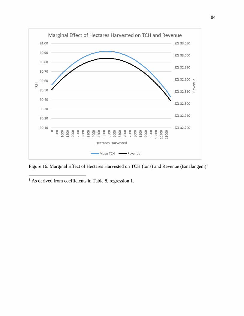
84

Figure 16. Marginal Effect of Hectares Harvested on TCH (tons) and Revenue (Emalangeni)1

1 As derived from coefficients in Table 8, regression 1.

SZL 32,700

SZL 32,750

SZL 32,800

SZL 32,850

SZL 32,900

SZL 32,950

SZL 33,000

SZL 33,050

90.10

90.20

90.30

90.40

90.50

90.60

90.70

90.80

90.90

91.00

0

50

0

10

00

15

00

20

00

25

00

30

00

35

00

40

00

45

00

50

00

55

00

60

00

65

00

70

00

75

00

80

00

85

00

90

00

95

00

10

00

0

10

50

0

11

00

0

Rev

enu

e

TCH

Hectares Harvested

Marginal Effect of Hectares Harvested on TCH and Revenue

Mean TCH Revenue

85

Figure 17. Marginal Effect of Hectares Harvested on Sucrose Percentage and Revenue

(Emalangeni)1

1 As derived from coefficients in Table 9, regression 1.

SZL 32,500

SZL 32,600

SZL 32,700

SZL 32,800

SZL 32,900

SZL 33,000

SZL 33,100

SZL 33,200

SZL 33,300

SZL 33,400

SZL 33,500

SZL 33,600

13.95%

14.00%

14.05%

14.10%

14.15%

14.20%

14.25%

14.30%

14.35%

14.40%

14.45%0

50

0

10

00

15

00

20

00

25

00

30

00

35

00

40

00

45

00

50

00

54

22

60

00

65

00

70

00

75

00

80

00

85

00

90

00

95

00

10

00

0

10

50

0

11

00

0

Rev

enu

e

Sucr

ose

Per

cen

tage

Hectares Harvested

Marginal Effect of Hectares Harvested on Sucrose Percentage and Revenue

Mean Sucrose Percentage Revenue

86

Figure 18. Marginal Effect of Age on TCH (tons) and Revenue (Emalangeni)1

1 As derived from coefficients from Table 14.

SZL 29,000

SZL 30,000

SZL 31,000

SZL 32,000

SZL 33,000

SZL 34,000

SZL 35,000

80

82

84

86

88

90

92

94

96

98

1 2 3 4 5 6 7 8 9 10 11 12 13 14 15 16 17 18 19 20

Rev

enu

e

TCH

Cane Age (months)

Marginal Effect of Age on TCH and Revenue

Mean TCh Revenue

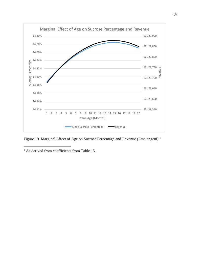
87

Figure 19. Marginal Effect of Age on Sucrose Percentage and Revenue (Emalangeni) 1

1 As derived from coefficients from Table 15.

SZL 29,550

SZL 29,600

SZL 29,650

SZL 29,700

SZL 29,750

SZL 29,800

SZL 29,850

SZL 29,900

14.12%

14.14%

14.16%

14.18%

14.20%

14.22%

14.24%

14.26%

14.28%

14.30%

1 2 3 4 5 6 7 8 9 10 11 12 13 14 15 16 17 18 19 20

Rev

enu

e

Sucr

ose

Per

cen

tage

Cane Age (Months)

Marginal Effect of Age on Sucrose Percentage and Revenue

Mean Sucrose Percentage Revenue

88

References

aWhere. (2017). Retrieved from http://www.awhere.com/

Barnabás, B., Jäger, K., & Fehér, A. (2008). The effect of drought and heat stress on

reproductive processes in cereals. Plant, Cell and Environment, 31(1), 11–38.

https://doi.org/10.1111/j.1365-3040.2007.01727.x

Bioenergy and Food Security Projects, & FAO. (2013). Swaziland BEFS Country Brief.

Blackburn, F. (1984). Sugar-cane. Longman Group Limited.

Christie, C. J., Langston, M., Todd, A., Hutchings, J., & Elliott, A. (2008). Energy Requirements

and perceived body discomfort of the various sub tasks of manual sugar cane harvesting: a

pilot study. Ergonomics SA, 20(2), 26–33. Retrieved from https://0-search-proquest-

com.library.uark.edu/docview/213836488?pq-origsite=summon

Clements, H. F. (1980). Sugarcane crop logging and crop control: Principles and practices.

University Press Hawaii, Honolulu.

Das, U. K. (1933). Measuring production in terms of temperature. Hawaiian Planters Record,

137, 32–53.

Deressa, T., Hassan, R., & Poonyth, D. (2005). Measuring the Impact of Climate Change on

South African Agriculture: the Case of Sugarcane Growing Regions. Agrekon, 44(4), 524–

542. https://doi.org/10.1080/03031853.2005.9523726

Ebrahim, M. K., Zingsheim, O., El-Shourbagy, M. N., Moore, P. H., & Komor, E. (1998).

Growth and sugar storage in sugarcane grown at temperatures below and above optimum.

Journal of Plant Physiology, 153(5–6), 593–602. https://doi.org/10.1016/S0176-

1617(98)80209-5

Economic Census 2011: Phase 1 Report. (2011). Central Statistical Office Swaziland.

https://doi.org/http://www.statistics.gov.my/portal/download_Manufacturing/files/BE/BE20

11_Manufacturing.pdf

Eswatini Economic Policy Analysis and Research Centre. (2017). Swaziland Economic

Conference: Post Conference Report.

Eswatini Sugar Assocation. (2016). Facts and Figures (Industry). Retrieved from

http://www.ssa.co.sz/facts-and-figures-industry/?hilite=%2235%25%22

Falola, T., & Jean-Jacques, D. (Eds.). (2016). Africa: An Encyclopedia of Culture and Society

(1st ed.). ABC-CLIO. Retrieved from https://0-search-credoreference-

com.library.uark.edu/content/title/abcclioacas?tab=contents

89

Food and Agriculture Organization of the United Nations. (n.d.). Swaziland looks to a revitalized

agriculture sector. Retrieved October 6, 2018, from http://www.fao.org/in-action/swaziland-

looks-to-a-revitalized-agriculture-sector/en/

Food and Agriculture Organization, & Office of Evaluation. (2011). Swaziland Agricultural

Development Programme (SADP). Retrieved from http://www.fao.org/3/a-bd203e.pdf

Glasziou, K. T., Bull, T. A., Hatch, M. D., & Whiteman, P. C. (1965). Physiology of Sugar-Cane

VII. Effects of temperature, photoperiod duration, and diurnal and seasonal temperature

changes on growth and ripening. Australian Journal of Biological Sciences, 18, 53–66.

https://doi.org/10.1038/189629b0

Government of Swaziland, UN Office for the Coordination of Humanitarian Affairs, & UN

Country Team in Swaziland. (2016). Swaziland: Humanitarian Needs Overview. Retrieved

from https://reliefweb.int/report/swaziland/swaziland-humanitarian-needs-overview-2016

Gowing, D. P. (1977). Observations on cane ripening in the Iranian winter. Proc Int Soc Sugar

Cane Technology, 16.

Grand Growth phase. (n.d.). Retrieved October 17, 2017, from

http://www.sugarcanecrops.com/crop_growth_phases/grand_growth_phase/

Hasanuzzaman, M., Nahar, K., Alam, M. M., Roychowdhury, R., & Fujita, M. (2013).

Physiological, Biochemical, and Molecular Mechanisms of Heat Stress Tolerance in Plants.

International Journal of Molecular Sciences, 14(5), 9643–9684.

https://doi.org/10.3390/ijms14059643

Hatch, M. D., & Glasziou, K. T. (1963). Sugar Accumulation Cycle in Sugar Cane. II.

Relationship of Invertase Activity to Sugar Content & Growth Rate in Storage Tissue of

Plants Grown in Controlled Environments. Plant Physiology, 38(3), 344–348.

Hess, T. M., Sumberg, J., Biggs, T., Georgescu, M., Haro-Monteagudo, D., Jewitt, G., … Knox,

J. W. (2016). A sweet deal? Sugarcane, water and agricultural transformation in Sub-

Saharan Africa. Global Environmental Change, 39, 181–194.

https://doi.org/10.1016/j.gloenvcha.2016.05.003

Inman-Bamber, N. G., & Smith, D. M. (2005). Water relations in sugarcane and response to

water deficits. Field Crops Research, 92(2–3 SPEC. ISS.), 185–202.

https://doi.org/10.1016/j.fcr.2005.01.023

Intergovernmental Panel on Climate Change (IPCC). (2007). Climate Change 2007: Synthesis

Report (Vol. 4). https://doi.org/10.1256/004316502320517344

Intergovernmental Panel on Climate Change (IPCC). (2014). Climate Change 2014: Synthesis

Report. https://doi.org/10.1017/CBO9781107415324

Jahan, S. (2016). Human Development Report 2016. United Nations Development Programme.

https://doi.org/eISBN: 978-92-1-060036-1

90

Keating, B. A., Robertson, M. J., Muchow, R. C., & Huth, N. I. (1999). Modelling sugarcane

production systems I. Development and performance of the sugarcane module. Field Crops

Research, 61(3), 253–271.

Knox, J. W., Rodríguez Díaz, J. A., Nixon, D. J., & Mkhwanazi, M. (2010). A preliminary

assessment of climate change impacts on sugarcane in Swaziland. Agricultural Systems,

103(2), 63–72. https://doi.org/10.1016/j.agsy.2009.09.002

Lule, E., Haacker, M., & World Bank. (2011). Fiscal Dimension of HIV/AIDS in Botswana,

South Africa, Swaziland, and Uganda: Experiences from Botswana, South Africa,

Swaziland, and Uganda. World Bank Publications.

Martin, J. P., & Eckart, R. C. (1933). The effect of various intensities of light on the growth of

the H109 variety of sugarcane. Hawaiian Planters Record, 37, 53–66.

Masuku, M. B. (2011). Determinants of Sugarcane Profitability : The Case of Smallholder Cane

Growers in Swaziland. Asian Journal of Agricultural Sciences, 3(3), 210–214.

Masuku, M. B., Kibrige, D., & Singh, A. S. (2015). IMPACT OF HIV AND AIDS ON

AGRICULTURAL PRODUCTION IN SWAZILAND : STRATEGIES FOR

MITIGATION. International Journal of Economics, Commerce and Managment, III(3), 1–

14.

Matondo, J. I., Graciana, P., & Msibi, K. M. (2004). Evaluation of the impact of climate change

on hydrology and water resources in Swaziland: Part I. Physics and Chemistry of the Earth,

29, 1181–1191.

Ministry of Labour and Social Security. (2010). The Swaziland Integrated Labour Force Survey

Report 2010. Retrieved from http://www.swazistats.org.sz/images/reports/Labour Force

Survey Report 2010.pdf

Moore, P. H., & Botha, F. C. (2013). Sugarcane: Physiology, Biochemistry, and Biology. John

Wiley & Sons, Inc. https://doi.org/10.1002/9781118771280

Muwanga, F. T. (2004). A Systematic Review of the Economic Impact of HIV/AIDS on

Swaziland. Johannesburg: University of Witwatersrand.

National Disaster Management Agency. (2016). National Drought Emergency Mitigation and

Adaptation Plan (NERMAP) 2016-2017. Retrieved from

https://www.humanitarianresponse.info/sites/www.humanitarianresponse.info/files/docume

nts/files/swaziland_national_emergency_response_mitigation_and_adaptation_plannermap1

_1-2.pdf

Pound, J., Michicels, J., & Bonaficio, R. (2015). FAO/WFP Crop and Food Security Assessment

Mission To Swaziland. Retrieved from

http://www.fao.org/docrep/012/ak346e/ak346e00.pdf

91

Reinhard, S., Knox Lovell, C. A., & Thijssen, G. J. (2000). Environmental efficiency with

multiple environmentally detrimental variables; estimated with SFA and DEA. European

Journal of Operational Research, 121(2), 287–303. https://doi.org/10.1016/S0377-

2217(99)00218-0

Reza, M. S., Riaza, M. H., & Khan, M. M. H. (2016). Productivity and profitability of sugarcane

production in Northern Bangladesh. Indian Journal of Commerce and Management Studies,

7(1).

Royal Swaziland Sugar Corporation - Operations. (n.d.). Retrieved May 7, 2018, from

http://www.rssc.co.sz/operations/agriculture/

RStudio Team (2016). RStudio: Integrated Development for R. RStudio, Inc., Boston, MA URL

http://www.rstudio.com/.

R Core Team (2017). R: A language and environment for statistical computing. R Foundation for

Statistical Computing, Vienna, Austria. URL https://www.R-project.org/.

Ryker, T. C., & Edgerton, C. W. (1931). Studies on sugar cane roots. Louisiana Agricultural

Experiment Station Bull, 223, 36–39.

Sanders, M. S., & McCormick, E. J. (1993). Human factors in engineering and design (7th ed.).

New York: McGraw-Hill.

Sartorius, G. B. . (1929). Low-temperature injury to stored sugarcane. Journal of Agricultural

Research, 38, 195–203.

Sikuka, W., & Torry, J. (2017). Swaziland Sugar Annual: The supply and demand of sugar in

Swaziland. Pretoria.

Srivastava, S., Pathak, A., Gupta, P., Shrivastava, A., & Srivastava, A. (2012). Hydrogen

peroxide-scavenging enzymes impart tolerance to high temperature induced oxidative stress

in sugarcane. Journal of Environmental Biology, 33(3), 657–661.

Swaziland Cane Growers Association. (2017). SCGA Annual Report 2016/2017. Retrieved from

http://www.scga.co.sz/images/ReducedPDF.compressedAnnualReport.pdf

Swaziland Sugar Association. (2016). Integrated Annual Report.

https://doi.org/10.1039/c1dt90165f

Swaziland Sugar Association. (2017). Sugar Industry. Retrieved January 3, 2017, from

http://www.ssa.co.sz/sugar-industry/

Terry, A., & Ogg, M. (2016). Restructuring the Swazi Sugar Industry: The Changing Role and

Political Significance of Smallholders. Journal of Southern African Studies.

https://doi.org/10.1080/03057070.2016.1190520

Thabethe, L. S. (2013). Estimation of technical, economic, and allocative efficiencies in

sugarcane production in South Africa: A case study of Mpumalanga growers. University of

Pretoria Dissertations.

92

Topouzis, D. (2003). Addressing the Impact of HIV/AIDS on Ministries of Agriculture: Focus on

Eastern and Southern Africa. Retrieved from

http://www.fao.org/docrep/005/Y4636E/y4636e00.htm#Contents

Ulandssekretariatet LO/FTF Council. (2012). Swaziland – Labour Market Profile 2012.

United Nations Conference on Trade and Development. (2000). Policies for Small-Scale Sugar

Cane Growing in Swaziland. Retrieved from

http://unctad.org/en/Docs/poitcdcomd28.en.pdf

Verret, J. A., & Das, U. K. (1927). Rate of cane growth at various ages. Hawaiian Planters

Record, 31, 314–320.

Watkins, K. (2006). Human Development Report 2006 - Beyond scarcity: Power, poverty and

the global water crisis. United Nations Development Programme (Vol. 28).

https://doi.org/10.1016/S1352-0237(02)00387-8

Wickham, H. ggplot2: Elegant Graphics for Data Analysis. Springer-Verlag New York, 2009

World Health Organization. (2017). Global Health Observatory Data Repository. Retrieved from

http://apps.who.int/gho/data/view.main.22500

Yusuf, G., & Purokayo, S. G. (2012). The Effects of HIV / AIDS Scourge on Production and

Income among Rural Households in Adamawa State of Nigeria. Global Journal of Health

Science, 4(1), 245–252. https://doi.org/10.5539/gjhs.v4n1p245

Zhao, D., & Li, Y.-R. (2015). Climate Change and Sugarcane Production: Potential Impact and

Mitigation Strategies. International Journal of Agronomy, 1–10.

https://doi.org/10.1155/2015/547386

Zingaretti, S. M., Rodrigues, F. A., da Graça, J. P., Pereira, L. D. M., & Lourenço, M. V. (2012).

Sugarcane Responses at Water Deficit Conditions. Water Stress, 255–276.

https://doi.org/10.5772/1419

93

Appendices

Appendix 1

Table 10b. Complete listing Farmer ID

(Cont.)

IDM002 -26.107** -25.949**

(10.925) (11.429)

IDM003 -0.324 -0.598

(11.190) (11.706)

IDM004 -11.835 -11.885

(11.190) (11.706)

IDM005 -3.800 -3.926

(11.190) (11.706)

IDM006 -14.707 -14.110

(10.928) (11.443)

IDM007 -12.696 -12.710

(11.193) (11.709)

IDM008 -34.875*** -34.909***

(10.925) (11.429)

IDM009 -7.493 -7.707

(11.191) (11.707)

IDM010 -16.423 -18.191

(11.517) (12.048)

IDM011 -34.792*** -35.348***

(10.925) (11.428)

IDM012 -10.958 -11.454

(10.924) (11.428)

IDM013 -48.671*** -49.379***

(11.192) (11.708)

IDM014 -10.097 -10.504

(10.702) (11.196)

IDM015 0.032 -0.251

(10.703) (11.196)

IDM016 -42.352*** -41.815***

(11.930) (12.501)

IDM017 -24.669** -23.745**

(11.518) (12.059)

IDM019 -34.453*** -34.629***

(10.925) (11.428)

IDM020 -29.224** -29.515**

(11.515) (12.046)

IDM021 -48.803*** -48.589***

(11.918) (12.467)

IDM022 -20.571* -21.033*

(10.925) (11.428)


(Cont.)

IDM023 32.402*** 31.897***

(10.926) (11.432)

IDM024 -10.919 -11.180

(10.703) (11.196)

IDM025 34.678*** 34.223***

(11.190) (11.705)

IDM026 -12.083 -12.653

(10.925) (11.428)

IDM027 -25.657** -26.237**

(10.925) (11.428)

IDM028 -17.576 -17.952

(10.703) (11.197)

IDM029 -21.828** -22.468**

(10.924) (11.427)

IDM030 6.557 6.507

(10.703) (11.199)

IDM031 -55.281*** -55.191***

(12.438) (13.011)

IDM032 -38.476*** -38.800***

(10.702) (11.196)

IDM033 -23.964** -24.149**

(10.702) (11.196)

IDM034 -28.041*** -28.398**

(10.702) (11.196)

IDM035 -39.655*** -40.512***

(11.192) (11.708)

IDM036 -23.563** -23.992**

(11.190) (11.705)

IDM037 -31.091*** -31.709***

(11.515) (12.046)

IDM038 17.445 16.639

(11.517) (12.048)

IDM039 -2.203 -2.951

(10.924) (11.428)

IDM040 -1.773 -2.626

(11.192) (11.707)

IDM041 -40.894*** -41.386***

(10.702) (11.196)

IDM042 -17.181 -17.717

(10.702) (11.196)

94


(Cont.)

IDM043 -12.792 -13.372

(10.702) (11.196)

IDM044 -63.099*** -63.484***

(12.441) (13.015)

IDM045 -26.723** -27.253**

(10.702) (11.196)

IDM046 -18.196* -18.688*

(10.702) (11.196)

IDM047 -21.835* -22.271*

(11.192) (11.708)

IDM048 -15.466 -16.237

(11.192) (11.707)

IDM049 -28.211*** -28.795***

(10.513) (10.998)

IDM050 14.465 12.668

(11.193) (11.709)

IDM051 1.989 -0.034

(11.923) (12.473)

IDM052 -20.691* -21.237*

(10.702) (11.196)

IDM053 -16.131 -16.875

(11.192) (11.707)

IDM054 -3.839 -4.190

(10.924) (11.428)

IDM055 -6.713 -7.254

(10.702) (11.196)

IDM056 -6.318 -6.857

(10.926) (11.430)

IDM057 4.789 3.961

(11.192) (11.707)

IDM058 -3.568 -3.367

(10.704) (11.200)

IDM059 -25.571** -25.894**

(10.926) (11.431)

IDM060 -8.884 -9.411

(10.702) (11.196)

IDM061 22.645** 21.862*

(11.192) (11.708)

IDM062 5.368 4.616

(11.192) (11.707)

IDM063 -40.829*** -41.295***

(10.702) (11.196)

IDM064 1.747 1.140


(Cont.)

(10.926) (11.431)

IDM065 -38.601*** -39.092***

(10.702) (11.196)

IDM066 5.250 4.850

(10.927) (11.435)

IDM067 11.223 10.734

(10.926) (11.432)

IDM068 5.789 5.516

(10.702) (11.196)

IDM069 21.398* 20.805*

(10.926) (11.431)

IDM070 4.461 3.968

(10.702) (11.196)

IDM071 13.613 12.811

(11.192) (11.708)

IDM072 1.475 0.673

(10.924) (11.427)

IDM073 -24.644** -25.468**

(11.192) (11.709)

IDM074 -5.834 -6.405

(10.926) (11.431)

IDM075 25.676** 24.869**

(11.192) (11.709)

IDM076 -9.747 -10.306

(10.703) (11.196)

IDM077 4.575 4.040

(10.702) (11.196)

IDM078 -1.462 -2.117

(11.192) (11.708)

IDM079 -2.995 -3.684

(10.924) (11.427)

IDM080 4.170 3.391

(10.925) (11.428)

IDM081 1.079 1.090

(11.518) (12.050)

IDM082 4.760 4.022

(10.924) (11.427)

IDM083 -32.644*** -34.416***

(11.517) (12.049)

IDM084 0.117 -0.609

(10.924) (11.428)

IDM085 -47.534*** -48.781***

(11.193) (11.709)

IDM086 15.405 14.694

95


(Cont.)

(10.924) (11.427)

IDM087 -44.913*** -44.956***

(14.110) (14.764)

IDM088 9.529 8.823

(11.192) (11.708)

IDM089 8.728 8.024

(10.924) (11.427)

IDM090 3.356 3.181

(10.703) (11.197)

IDM091 -1.269 -1.969

(10.924) (11.427)

IDM092 -33.960*** -34.627***

(10.924) (11.427)

IDM093 6.300 5.543

(10.924) (11.427)

IDM094 -5.330 -5.683

(10.702) (11.196)

IDM095 3.542 2.807

(10.924) (11.427)

IDM096 -13.894 -14.557

(10.924) (11.427)

IDM097 10.076 9.545

(10.702) (11.196)

IDM098 17.722 16.897

(11.192) (11.708)

IDM099 -14.675 -15.387

(10.924) (11.428)

IDM100 9.740 9.563

(10.703) (11.197)

IDM101 1.738 0.918

(11.192) (11.708)

IDM102 -6.896 -7.440

(10.702) (11.196)

IDM103 8.548 7.849

(10.924) (11.427)

IDM104 -21.884** -22.356**

(10.702) (11.196)

IDM105 -0.929 -1.454

(10.702) (11.196)

IDM106 -8.971 -9.713

(10.924) (11.427)

IDM107 -25.832** -26.559**

(10.924) (11.427)

IDM108 10.690 9.920


(Cont.)

(10.924) (11.427)

IDM109 -2.619 -3.179

(10.702) (11.196)

IDM110 4.421 3.850

(10.702) (11.196)

IDM111 7.132 6.808

(10.703) (11.196)

IDM112 -12.804 -12.497

(10.928) (11.440)

IDM113 12.993 12.509

(11.190) (11.705)

IDM114 -36.876*** -37.111***

(10.925) (11.428)

IDM115 -17.598 -18.344

(10.924) (11.427)

IDM116 -5.984 -6.655

(10.924) (11.427)

IDM117 -32.878*** -33.029***

(11.516) (12.047)

IDM118 7.378 6.751

(10.924) (11.427)

IDM119 24.259* 22.426*

(12.443) (13.018)

IDM120 -0.226 -0.613

(10.702) (11.196)

IDM121 -48.187*** -48.275***

(10.926) (11.430)

IDM122 -15.785 -14.883

(11.196) (11.722)

IDM123 -2.658 -3.226

(10.924) (11.427)

IDM124 9.351 8.624

(10.924) (11.427)

IDM125 -16.243 -16.887

(11.192) (11.707)

IDM126 -3.833 -4.013

(10.702) (11.196)

IDM127 1.750 1.050

(10.924) (11.427)

IDM128 -11.373 -12.040

(10.924) (11.427)

IDM129 0.519 0.548

(11.192) (11.709)

IDM130 -49.931*** -50.470***

96


(Cont.)

(11.194) (11.711)

IDM131 -31.055** -30.289**

(12.438) (13.012)

IDM132 -42.581*** -42.591***

(11.192) (11.708)

IDM133 -20.592* -19.967

(11.925) (12.477)

IDM134 -31.446*** -32.274***

(11.192) (11.708)

IDM135 -42.235*** -42.409***

(11.194) (11.711)

IDM136 -47.243*** -47.847***

(10.924) (11.427)

IDM137 -71.253*** -71.653***

(10.702) (11.196)

IDM138 -46.250*** -46.387***

(10.927) (11.432)

IDM139 -31.719*** -32.107***

(10.702) (11.196)

IDM140 -30.866*** -31.055***

(10.927) (11.431)

IDM142 -46.743*** -47.126***

(10.924) (11.428)

IDM143 -59.997*** -60.770***

(11.517) (12.048)

IDM144 -22.853** -23.256**

(10.702) (11.196)

IDM145 -28.025*** -28.400**

(10.703) (11.196)

IDM146 -17.699 -18.268

(10.924) (11.428)

IDM147 -11.984 -12.501

(11.194) (11.711)

IDM148 -3.446 -4.200

(10.924) (11.427)

IDM149 6.531 6.096

(10.703) (11.196)

IDM150 -9.383 -10.150

(11.192) (11.707)

IDM151 -17.128 -17.782

(10.924) (11.428)

IDM152 -20.129* -20.793*

(10.924) (11.427)

IDM153 -14.419 -14.849


(Cont.)

(10.702) (11.196)

IDM154 -26.976** -27.437**

(10.924) (11.428)

IDM155 2.483 1.810

(10.925) (11.428)

IDM156 1.016 0.424

(10.924) (11.428)

IDM157 -4.212 -4.710

(10.702) (11.196)

IDM158 -11.063 -11.445

(10.924) (11.428)

IDM159 -20.493* -20.966*

(10.702) (11.196)

IDM160 -15.686 -16.319

(10.924) (11.427)

IDM161 -4.229 -4.701

(10.702) (11.196)

IDM162 11.497 10.954

(10.925) (11.428)

IDM163 -44.722*** -44.846***

(10.927) (11.431)

IDM164 -1.162 -1.753

(10.924) (11.427)

IDM165 13.383 12.801

(10.924) (11.427)

IDM166 -15.880 -16.356

(10.702) (11.196)

IDM167 -33.583*** -33.998***

(10.702) (11.196)

IDM168 -1.877 -1.864

(11.192) (11.709)

IDM169 -17.581 -18.022

(10.702) (11.196)

IDM170 -5.540 -6.764

(11.518) (12.050)

IDM171 4.649 4.055

(10.924) (11.428)

IDM172 -27.589** -28.867**

(11.520) (12.053)

IDM174 -23.020* -22.483

(13.138) (13.748)

IDM175 0.877 0.329

(10.924) (11.427)

IDM176 -15.871 -16.289

97


(Cont.)

(10.702) (11.196)

IDM177 -23.204** -23.509**

(11.190) (11.705)

IDM178 -19.393* -19.877*

(10.924) (11.428)

IDM179 -0.830 -1.140

(10.926) (11.430)

IDM180 -16.303 -15.317

(11.522) (12.058)

IDM181 -1.264 -1.728

(10.702) (11.196)

IDM182 -30.414*** -31.144***

(11.517) (12.049)

IDM183 68.954*** 68.473***

(10.926) (11.430)

IDM184 -42.827*** -43.238***

(10.702) (11.196)

IDM186 -7.120 -7.595

(10.702) (11.196)

IDM187 -7.161 -7.685

(10.702) (11.196)

IDM188 -28.295*** -28.949**

(10.924) (11.427)

IDM189 -30.989*** -31.429***

(10.926) (11.430)

IDM190 -4.548 -5.162

(11.194) (11.711)

IDM191 23.969** 23.476**

(10.925) (11.428)

IDM192 -5.509 -6.037

(10.924) (11.428)

IDM193 -13.399 -13.714

(10.703) (11.197)

IDM194 -19.607* -20.346*

(10.924) (11.427)

IDM195 -26.718** -27.049**

(11.192) (11.708)

IDM196 -6.624 -7.371

(10.924) (11.427)

IDM197 -1.985 -2.728

(10.924) (11.427)

IDM198 -15.372 -15.946

(10.925) (11.428)

IDM199 -20.182* -21.358*


(Cont.)

(11.517) (12.049)

IDM200 -27.847** -28.553**

(11.923) (12.474)

IDM201 -25.021** -25.111*

(12.444) (13.023)

IDM202 -12.807 -12.753

(10.704) (11.203)

IDM203 -41.015*** -41.629***

(10.924) (11.427)

IDM204 -26.409** -27.140**

(11.192) (11.707)

IDM205 -7.741 -8.247

(11.517) (12.049)

IDM206 -12.938 -12.817

(11.521) (12.053)

IDM207 -23.719* -24.679*

(12.444) (13.020)

IDM209 -32.683*** -32.622***

(11.200) (11.721)

IDM210 -17.701 -17.669

(10.928) (11.436)

IDM211 -17.377 -18.094

(11.923) (12.474)

IDM212 -18.284* -18.735*

(10.702) (11.196)

IDM213 -9.068 -9.688

(10.926) (11.430)

IDM214 -10.355 -10.367

(10.929) (11.435)

IDM215 -10.548 -10.450

(10.703) (11.199)

IDM216 9.973 9.665

(10.926) (11.431)

IDM217 -0.834 -1.116

(10.927) (11.431)

IDM218 -35.274*** -35.699***

(11.519) (12.051)

IDM219 -50.753*** -50.080***

(11.199) (11.722)

IDM220 -17.371 -19.316

(11.923) (12.473)

IDM221 -26.049** -26.104**

(11.520) (12.066)

IDM222 -22.209** -23.263**

98


(Cont.)

(11.194) (11.712)

IDM223 -13.979 -15.030

(11.194) (11.712)

IDM224 -20.913* -21.640*

(10.924) (11.427)

IDM225 -21.386** -21.833*

(10.702) (11.196)

IDM226 10.622 10.064

(10.924) (11.427)

IDM227 -36.967*** -37.620***

(11.515) (12.046)

IDM228 -12.573 -13.184

(10.924) (11.427)

IDM229 -40.578*** -40.990***

(10.702) (11.196)

IDM230 -18.831* -19.277*

(10.702) (11.196)

IDM231 -40.822*** -41.755***

(11.517) (12.049)

IDM232 -41.501*** -42.133***

(11.191) (11.707)

IDM233 1.971 1.433

(10.702) (11.196)

IDM234 -25.083** -26.021**

(10.926) (11.431)

IDM235 -11.682 -12.210

(11.192) (11.707)

IDM236 -41.854*** -42.355***

(10.924) (11.427)

IDM237 -13.266 -13.613

(10.703) (11.197)

IDM238 -48.078*** -48.718***

(10.924) (11.427)

IDM239 -39.764*** -39.602***

(10.929) (11.435)

IDM240 -29.497*** -29.839**

(11.190) (11.705)

IDM241 -14.515 -14.755

(10.927) (11.432)

IDM242 -14.501 -15.063

(11.191) (11.707)

IDM243 -9.395 -9.750

(10.702) (11.196)

IDM244 -16.330 -16.903


(Cont.)

(10.924) (11.428)

IDM245 -21.632** -21.169*

(10.931) (11.439)

IDM246 -16.299 -16.690

(10.926) (11.431)

IDM247 -8.021 -8.705

(11.192) (11.708)

IDM248 -29.747*** -29.996**

(11.194) (11.711)

IDM249 -40.845*** -40.991***

(10.926) (11.431)

IDM250 -21.114* -21.374*

(10.926) (11.430)

IDM251 -26.375** -26.556**

(11.194) (11.711)

IDM252 -1.496 -0.829

(12.438) (13.011)

IDM253 -51.243*** -51.849***

(11.194) (11.711)

IDM254 -35.701*** -36.177***

(11.192) (11.708)

IDM255 -8.142 -8.061

(11.518) (12.050)

IDM256 -27.469** -27.881**

(10.702) (11.196)

IDM257 -29.528*** -29.945***

(10.702) (11.196)

IDM258 -25.278** -24.732**

(11.202) (11.727)

IDM259 -15.602 -16.519

(11.192) (11.708)

IDM260 -11.875 -13.722

(12.443) (13.018)

IDM261 -19.621* -20.200*

(10.924) (11.427)

IDM262 -33.189*** -33.324***

(10.927) (11.434)

IDM263 -39.507*** -40.018***

(11.518) (12.052)

IDM264 -36.765*** -36.986***

(11.192) (11.709)

IDM265 -42.794*** -43.238***

(10.924) (11.428)

IDM266 -23.455** -23.866**

99


(Cont.)

(10.704) (11.198)

IDM267 -37.238*** -37.212***

(10.927) (11.433)

IDM268 -38.933*** -39.257***

(10.926) (11.430)

IDM269 -36.841*** -38.424***

(11.923) (12.473)

IDM270 -31.877*** -32.340***

(10.702) (11.196)

IDM271 -33.779*** -34.447***

(10.924) (11.427)

IDM272 -47.352*** -47.792***

(10.926) (11.430)

IDM273 -26.676** -27.095**

(10.703) (11.196)

IDM274 -35.769*** -36.001***

(10.925) (11.428)

IDM275 -12.622 -13.303

(10.924) (11.427)

IDM276 -49.047*** -49.451***

(10.924) (11.428)

IDM277 -40.043*** -40.656***

(10.924) (11.427)

IDM278 -0.471 -1.100

(10.924) (11.427)

IDM279 -29.979*** -30.029***

(10.704) (11.199)

IDM280 -74.935*** -68.301***

(13.186) (14.287)

IDM281 -21.722** -22.015**

(10.703) (11.196)

IDM282 -40.168*** -38.319***

(11.523) (12.079)

IDM283 -7.984 -8.764

(10.924) (11.427)

IDM284 8.134 7.341

(10.924) (11.427)

IDM285 -9.185 -10.382

(11.518) (12.049)

IDM286 -3.776 -4.419

(10.924) (11.427)

IDM287 -27.080** -27.170**

(11.192) (11.709)

IDM288 -38.148*** -37.935***


(Cont.)

(11.192) (11.709)

IDM289 -17.092 -17.623

(10.702) (11.196)

IDM290 -34.225*** -35.140***

(11.517) (12.049)

IDM291 -37.980*** -37.805***

(11.921) (12.471)

IDM292 -28.183*** -28.483**

(10.926) (11.430)

IDM293 -7.487 -8.065

(10.702) (11.196)

IDM294 -27.935*** -28.478**

(10.702) (11.196)

IDM295 -12.505 -12.966

(10.702) (11.196)

IDM296 -24.692** -25.463**

(10.924) (11.427)

IDM297 -10.390 -11.147

(10.924) (11.427)

IDM298 7.365 6.822

(10.702) (11.196)

IDM299 -6.402 -6.890

(10.702) (11.196)

IDM300 -2.528 -2.800

(10.702) (11.196)

IDM301 -14.499 -14.927

(10.702) (11.196)

IDM302 9.797 9.423

(10.702) (11.196)

IDM303 -30.811*** -30.764**

(11.521) (12.057)

IDM304 -35.173*** -35.330***

(10.928) (11.435)

IDM305 -17.992* -18.044

(10.926) (11.431)

IDM306 -24.088** -24.764**

(10.924) (11.427)

IDM307 0.203 -0.366

(10.702) (11.196)

IDM308 12.721 11.963

(10.924) (11.427)

IDM309 -36.438*** -36.727***

(10.703) (11.197)

IDM310 -16.275 -16.614

100


(Cont.)

(10.702) (11.196)

IDM311 -20.225* -20.649*

(10.926) (11.430)

IDM312 -22.855** -22.223*

(11.516) (12.048)

IDM313 -4.534 -5.214

(10.924) (11.427)

IDM314 -17.268 -17.548

(11.193) (11.709)

IDM315 -19.686* -19.468

(11.518) (12.050)

IDM316 -22.281** -22.901**

(10.924) (11.427)

IDM317 -29.662*** -29.983***

(10.925) (11.428)

IDM318 9.370 8.811

(10.924) (11.428)

IDM319 1.362 0.778

(10.924) (11.428)

IDM320 -12.577 -13.708

(11.518) (12.050)

IDM321 -17.496 -18.072

(10.925) (11.428)

IDM343 -0.415 -2.082

(12.443) (13.018)

IDM348 -0.335 -1.990

(12.443) (13.018)

IDM349 11.823 10.153

(12.443) (13.018)

IDM363 -29.735** -32.114**

(13.136) (13.744)

IDS001 12.638

(13.631)

IDS002 30.131** 17.342***

(13.631) (6.220)

IDS005 2.997 -9.925

(13.631) (6.240)

IDS006 5.016 -7.741

(13.631) (6.239)

IDS008 -17.325 -33.876***

(15.469) (7.714)

IDS009 16.505 3.480

(13.453) (6.087)

IDS011 -1.926 -16.249***


(Cont.)

(13.457) (6.156)

IDS012 19.893 6.777

(13.454) (6.089)

IDS013 -11.565 -23.321***

(13.659) (6.398)

IDS014 -6.741 -20.152***

(13.634) (6.240)

IDS015 4.666 -8.188

(13.453) (6.085)

IDS016 -14.281 -27.107***

(13.453) (6.085)

IDS018 -23.322 -36.052***

(16.306) (8.359)

IDS019 -28.632 -40.046***

(17.610) (9.329)

IDS021 -44.361*** -55.114***

(14.108) (6.622)

IDS022 5.924 -6.430

(13.631) (6.222)

IDS023 -21.597 -33.775***

(13.845) (6.421)

IDS024 -15.161 -27.773***

(13.631) (6.239)

IDS027 -22.654 -35.128***

(13.845) (6.401)

IDS028 3.992 -6.633

(13.845) (6.418)

IDS029 -1.457 -11.476

(14.868) (7.251)

IDS030 3.947 -8.896

(13.453) (6.085)

IDS031 -38.881*** -53.259***

(14.115) (6.629)

IDS032 39.062*** 25.536***

(13.848) (6.431)

IDS035 -17.833 -30.142***

(13.631) (6.223)

IDS037 -21.095 -33.889***

(16.306) (8.347)

IDS038 14.426 -1.852

(15.469) (7.678)

IDS041 -7.066 -18.031***

(14.439) (6.884)

IDS042 8.505 -2.422

101


(Cont.)

(14.439) (6.884)

IDS043 -6.949

(8.312)

IDU001 -6.177

(13.141)

IDU002 -3.824 2.362 (13.141) (9.297)

IDU003 -21.141 -14.313 (13.497) (9.629)

IDU004 -0.806 4.934 (13.141) (9.305)

IDU006 -25.957* -21.880** (13.965) (10.053)

IDU007 3.203 9.469 (13.497) (9.635)

IDU009 -17.341 -10.916 (13.497) (9.632)

IDU011 1.580 7.225 (13.142) (9.309)

IDU013 -2.139 3.700 (13.498) (9.656)

IDU014 -10.019 -6.339 (13.963) (10.053)

IDU015 1.418 7.561 (13.497) (9.640)

IDU016 19.062 25.123*** (13.141) (9.298)

IDU017 -17.794 -11.995 (13.142) (9.304)

IDU018 -12.678 -6.361 (13.497) (9.634)

IDU019 -24.941* -19.033** (13.141) (9.300)

IDU020 -25.258* -19.171** (13.141) (9.298)

IDU021 12.765 19.021** (13.497) (9.636)

IDU022 -9.129 -2.887 (13.497) (9.636)

IDU023 -8.197 -1.730 (13.497) (9.631)

IDU024 -4.757 2.974 (13.498) (9.640)

IDU025 -4.180 1.785


(Cont.)

(13.141) (9.299)

IDU026 8.425 17.170* (13.957) (10.060)

IDU027 -24.497* -18.744** (13.141) (9.305)

IDU028 -21.812* -15.827* (13.141) (9.299)

IDU029 -9.573 -3.206 (13.497) (9.633)

IDU030 -41.439*** -31.377*** (15.468) (11.437)

IDU031 -18.291 -12.044 (13.141) (9.309)

IDU032 8.564 16.127* (12.856) (9.040)

IDU033 -24.733* -17.463* (12.855) (9.043)

IDU034 7.046 14.929* (12.639) (8.860)

IDU035 15.025 23.485*** (12.853) (9.057)

IDU036 2.798 11.031 (12.622) (8.830)

IDU037 -11.972 -3.336 (13.140) (9.307)

IDU038 -21.947* -13.651 (12.852) (9.063)

IDU039 -16.291 -8.692 (13.957) (10.065)

IDU040 -40.838*** -34.982*** (13.500) (9.638)

IDU041 -17.767 -11.171 (13.496) (9.646)

IDU042 -5.460 3.121 (12.853) (9.054)

IDU043 -45.199*** -38.633*** (13.496) (9.647)

IDU044 3.243 11.267 (12.622) (8.831)

IDU045 -31.975** -29.566*** (14.581) (10.622)

IDU046 -16.467 -8.399 (12.622) (8.831)

IDU047 -15.295 -7.197

102


(Cont.)

(12.622) (8.830)

IDU048 -24.527* -16.308* (12.622) (8.830)

IDU049 -23.033* -19.428* (13.960) (10.056)

IDU050 -39.193*** -29.201*** (13.491) (9.651)

IDU051 -10.484 -1.906 (13.139) (9.319)

IDU052 120.898*** 125.492*** (13.500) (9.629)

IDU053 -28.194** -20.540** (13.138) (9.322)

IDU054 -22.766* -14.667* (12.622) (8.831)

IDU055 -25.389** -17.060* (12.852) (9.061)

IDU056 -7.393 0.542 (12.853) (9.050)

IDU057 -37.544*** -29.187*** (12.852) (9.060)

IDU059 -37.952*** -29.437*** (12.853) (9.055)

IDU060 -21.752* -14.015 (12.622) (8.840)

IDU062 -18.742 -9.832 (12.853) (9.050)

IDU064 -25.158* -16.145* (12.853) (9.050)

IDU065 -14.990 -8.349 (12.620) (8.843)

IDU067 -11.437 -3.478 (12.529) (8.792)

IDU068 -21.872* -14.540* (12.426) (8.663)

IDU069 -26.928** -19.368** (12.426) (8.656)

IDU070 -5.087 -2.379 (13.955) (10.067)

IDU071 -5.893 -5.162 (16.843) (12.643)

IDU072 -27.158** -22.738** (13.140) (9.311)

IDU073 -24.529** -16.932*


(Cont.)

(12.426) (8.656)

IDU075 -51.233*** -46.784*** (13.960) (10.066)

IDU076 -1.760 6.002 (12.427) (8.654)

IDU077 -2.873 4.424 (12.622) (8.831)

IDU078 -2.407 5.159 (12.430) (8.662)

IDU079 -26.179** -18.836** (12.427) (8.664)

IDU080 -37.765*** -30.906*** (13.138) (9.317)

IDU081 -37.374*** -32.598*** (13.963) (10.073)

IDU082 -46.740*** -40.162*** (12.620) (8.845)

IDU084 -24.397* -17.709* (12.851) (9.083)

IDU085 -19.072 -9.800 (13.169) (9.417)

IDU086 -31.755** -27.158*** (13.957) (10.114)

IDU087 -17.295 -13.034 (13.495) (9.655)

IDU088 -6.258 1.006 (12.427) (8.666)

IDU089 2.240 9.847 (12.426) (8.655)

IDU090 8.977 16.972* (12.618) (8.845)

IDU091 10.466 18.024** (12.426) (8.656)

IDU092 -25.114* -19.922** (12.857) (9.064)

IDU094 7.592 15.617* (12.849) (9.063)

IDU095 -2.512 5.507 (12.618) (8.844)

IDU097 -1.764 5.037 (12.851) (9.058)

IDU097 -17.953 0.011 (25.247) (19.895)

IDU098 1.564 7.685

103


(Cont.)

(13.137) (9.327)

IDU099 -19.068 -14.569 (13.495) (9.647)

IDU100 0.747 5.716 (14.586) (10.653)

IDU101 -12.320 -4.479 (12.849) (9.064)

IDU102 -11.863 -7.395 (13.495) (9.648)

IDU103 -4.869 -0.331 (13.495) (9.646)

IDU104 -5.139 -0.593 (13.140) (9.309)

IDU105 -8.073 -0.923 (12.851) (9.065)

IDU106 -25.066** -18.950** (12.635) (8.867)

IDU107 -10.314 -2.886 (12.426) (8.659)

IDU109 -34.071** -30.493** (16.840) (12.624)


(Cont.)

IDU110 -23.467* -14.226 (13.950) (10.095)

IDU112 -35.443*** -28.634*** (12.621) (8.840)

IDU114 23.293 36.299*** (14.569) (10.660)

IDU115 -22.733 -18.011* (13.952) (10.100)

IDU116 -17.898 -7.851

(13.487) (9.667)

IDU117 -1.991 2.853 (13.952) (10.094)

IDU118 -5.129 4.738 (13.486) (9.670)

IDU119 9.247 19.340** (13.487) (9.666)

IDU120 -19.947 -7.602 (14.564) (10.669)

IDU121 12.022 (10.675)

104

Appendix 2


(Cont.)

IDM004 -1.016** -1.015**

(0.462) (0.490)

IDM005 -0.344 -0.348

(0.462) (0.490)

IDM006 -0.657 -0.617

(0.451) (0.478)

IDM007 -1.159** -1.165**

(0.462) (0.490)

IDM008 0.040 0.027

(0.451) (0.478)

IDM009 0.290 0.279

(0.462) (0.490)

IDM010 0.011 -0.023

(0.475) (0.504)

IDM011 -0.565 -0.576

(0.451) (0.478)

IDM012 -0.483 -0.490

(0.451) (0.478)

IDM013 -0.844* -0.848*

(0.462) (0.490)

IDM014 -0.799* -0.813*

(0.442) (0.468)

IDM015 -0.784* -0.791*

(0.442) (0.468)

IDM016 -0.711 -0.646

(0.492) (0.523)

IDM017 -1.373*** -1.302***

(0.475) (0.504)

IDM019 -0.848* -0.853*

(0.451) (0.478)

IDM020 -0.694 -0.702

(0.475) (0.504)

IDM021 -1.487*** -1.496***

(0.492) (0.521)

IDM022 -0.396 -0.401

(0.451) (0.478)

IDM023 -0.757* -0.756

(0.451) (0.478)

IDM024 0.020 0.013

(0.442) (0.468)

IDM025 -0.066 -0.071

(0.462) (0.489)

IDM026 0.239 0.227


(Cont.)

(0.451) (0.478)

IDM027 0.286 0.273

(0.451) (0.478)

IDM028 -0.595 -0.610

(0.442) (0.468)

IDM029 -0.382 -0.398

(0.451) (0.478)

IDM030 -1.058** -1.045**

(0.442) (0.468)

IDM031 -1.813*** -1.819***

(0.513) (0.544)

IDM032 -1.309*** -1.318***

(0.442) (0.468)

IDM033 -0.485 -0.484

(0.442) (0.468)

IDM034 -0.675 -0.687

(0.442) (0.468)

IDM035 -0.591 -0.608

(0.462) (0.490)

IDM036 -0.648 -0.653

(0.462) (0.489)

IDM037 -0.855* -0.860*

(0.475) (0.504)

IDM038 -0.421 -0.428

(0.475) (0.504)

IDM039 -0.725 -0.744

(0.451) (0.478)

IDM040 -0.282 -0.302

(0.462) (0.490)

IDM041 -0.585 -0.605

(0.442) (0.468)

IDM042 -0.241 -0.264

(0.442) (0.468)

IDM043 -0.498 -0.522

(0.442) (0.468)

IDM044 -0.862* -0.851

(0.513) (0.544)

IDM045 -0.313 -0.335

(0.442) (0.468)

IDM046 -1.138** -1.159**

(0.442) (0.468)

IDM047 -0.888* -0.901*

(0.462) (0.490)

105


(Cont.)

IDM048 -1.038** -1.054**

(0.462) (0.490)

IDM049 -0.110 -0.128

(0.434) (0.460)

IDM050 -0.134 -0.167

(0.462) (0.490)

IDM051 -0.910* -0.954*

(0.492) (0.522)

IDM052 -0.125 -0.148

(0.442) (0.468)

IDM053 -0.996** -1.010**

(0.462) (0.490)

IDM054 -0.999** -0.995**

(0.451) (0.478)

IDM055 0.529 0.506

(0.442) (0.468)

IDM056 0.249 0.247

(0.451) (0.478)

IDM057 -0.450 -0.469

(0.462) (0.490)

IDM058 -0.630 -0.607

(0.442) (0.468)

IDM059 -1.029** -1.050**

(0.451) (0.478)

IDM060 -0.990** -1.012**

(0.442) (0.468)

IDM061 -0.789* -0.806*

(0.462) (0.490)

IDM062 -0.925** -0.938*

(0.462) (0.490)

IDM063 -1.018** -1.035**

(0.442) (0.468)

IDM064 -0.074 -0.080

(0.451) (0.478)

IDM065 -0.427 -0.447

(0.442) (0.468)

IDM066 0.071 0.081

(0.451) (0.478)

IDM067 -0.496 -0.494

(0.451) (0.478)

IDM068 -0.477 -0.482

(0.442) (0.468)

IDM069 -0.600 -0.621

(0.451) (0.478)

IDM070 -0.204 -0.225


(Cont.)

(0.442) (0.468)

IDM071 -0.467 -0.485

(0.462) (0.490)

IDM072 -0.723 -0.746

(0.451) (0.478)

IDM073 -0.312 -0.320

(0.462) (0.490)

IDM074 -0.653 -0.657

(0.451) (0.478)

IDM075 -0.140 -0.152

(0.462) (0.490)

IDM076 0.029 0.008

(0.442) (0.468)

IDM077 -0.532 -0.555

(0.442) (0.468)

IDM078 -0.878* -0.887*

(0.462) (0.490)

IDM079 0.349 0.331

(0.451) (0.478)

IDM080 -0.402 -0.423

(0.451) (0.478)

IDM081 -1.075** -1.097**

(0.475) (0.504)

IDM082 -0.666 -0.688

(0.451) (0.478)

IDM083 -0.238 -0.275

(0.475) (0.504)

IDM084 -0.724 -0.745

(0.451) (0.478)

IDM085 -0.435 -0.459

(0.462) (0.490)

IDM086 -0.673 -0.693

(0.451) (0.478)

IDM087 -2.234*** -2.270***

(0.582) (0.617)

IDM088 -0.951** -0.964**

(0.462) (0.490)

IDM089 -0.807* -0.826*

(0.451) (0.478)

IDM090 -0.518 -0.518

(0.442) (0.468)

IDM091 -0.758* -0.777

(0.451) (0.478)

IDM092 -1.051** -1.068**

(0.451) (0.478)

106


(Cont.)

IDM093 -0.703 -0.725

(0.451) (0.478)

IDM094 -0.518 -0.531

(0.442) (0.468)

IDM095 -0.693 -0.715

(0.451) (0.478)

IDM096 -0.587 -0.603

(0.451) (0.478)

IDM097 -0.405 -0.427

(0.442) (0.468)

IDM098 -0.775* -0.795

(0.462) (0.490)

IDM099 -0.366 -0.387

(0.451) (0.478)

IDM100 -1.304*** -1.305***

(0.442) (0.468)

IDM101 -0.594 -0.613

(0.462) (0.490)

IDM102 -0.991** -1.014**

(0.442) (0.468)

IDM103 -0.879* -0.897*

(0.451) (0.478)

IDM104 -0.806* -0.825*

(0.442) (0.468)

IDM105 -0.375 -0.396

(0.442) (0.468)

IDM106 -0.651 -0.673

(0.451) (0.478)

IDM107 -0.894** -0.914*

(0.451) (0.478)

IDM108 -0.928** -0.951**

(0.451) (0.478)

IDM109 -0.802* -0.825*

(0.442) (0.468)

IDM110 -1.044** -1.067**

(0.442) (0.468)

IDM111 -0.382 -0.392

(0.442) (0.468)

IDM112 -0.945** -0.901*

(0.451) (0.478)

IDM113 -1.003** -1.009**

(0.462) (0.489)

IDM114 -1.363*** -1.371***

(0.451) (0.478)

IDM115 -1.466*** -1.486***


(Cont.)

(0.451) (0.478)

IDM116 -0.337 -0.355

(0.451) (0.478)

IDM117 -1.646*** -1.653***

(0.475) (0.504)

IDM118 -0.526 -0.540

(0.451) (0.478)

IDM119 -0.464 -0.508

(0.513) (0.544)

IDM120 -0.490 -0.502

(0.442) (0.468)

IDM121 -1.301*** -1.304***

(0.451) (0.478)

IDM122 -1.601*** -1.558***

(0.462) (0.490)

IDM123 -0.171 -0.182

(0.451) (0.478)

IDM124 -0.016 -0.036

(0.451) (0.478)

IDM125 -1.416*** -1.422***

(0.462) (0.490)

IDM126 -2.059*** -2.057***

(0.442) (0.468)

IDM127 -1.366*** -1.383***

(0.451) (0.478)

IDM128 -0.310 -0.325

(0.451) (0.478)

IDM129 -0.571 -0.576

(0.462) (0.490)

IDM130 -1.723*** -1.721***

(0.462) (0.490)

IDM131 -1.542*** -1.525***

(0.513) (0.544)

IDM132 -1.375*** -1.372***

(0.462) (0.490)

IDM133 -1.342*** -1.339**

(0.492) (0.522)

IDM134 -1.345*** -1.356***

(0.462) (0.490)

IDM135 -0.787* -0.802

(0.462) (0.490)

IDM136 -0.939** -0.949**

(0.451) (0.478)

IDM137 -0.640 -0.652

(0.442) (0.468)

107


(Cont.)

IDM138 -1.576*** -1.578***

(0.451) (0.478)

IDM139 -1.776*** -1.790***

(0.442) (0.468)

IDM140 -1.458*** -1.462***

(0.451) (0.478)

IDM142 -0.528 -0.526

(0.451) (0.478)

IDM143 -1.605*** -1.613***

(0.475) (0.504)

IDM144 -1.879*** -1.891***

(0.442) (0.468)

IDM145 -0.712 -0.726

(0.442) (0.468)

IDM146 -0.823* -0.835*

(0.451) (0.478)

IDM147 -0.869* -0.881*

(0.462) (0.490)

IDM148 0.084 0.062

(0.451) (0.478)

IDM149 -0.406 -0.424

(0.442) (0.468)

IDM150 -0.889* -0.904*

(0.462) (0.490)

IDM151 -0.984** -1.001**

(0.451) (0.478)

IDM152 -1.006** -1.022**

(0.451) (0.478)

IDM153 -0.197 -0.213

(0.442) (0.468)

IDM154 -1.543*** -1.547***

(0.451) (0.478)

IDM155 -0.845* -0.858*

(0.451) (0.478)

IDM156 -0.420 -0.433

(0.451) (0.478)

IDM157 0.150 0.130

(0.442) (0.468)

IDM158 -1.109** -1.106**

(0.451) (0.478)

IDM159 -0.498 -0.517

(0.442) (0.468)

IDM160 -0.587 -0.602

(0.451) (0.478)

IDM161 -0.748* -0.767


(Cont.)

(0.442) (0.468)

IDM162 -0.675 -0.685

(0.451) (0.478)

IDM163 -1.466*** -1.478***

(0.451) (0.478)

IDM164 -0.607 -0.619

(0.451) (0.478)

IDM165 -0.664 -0.676

(0.451) (0.478)

IDM166 -1.143*** -1.161**

(0.442) (0.468)

IDM167 -0.687 -0.703

(0.442) (0.468)

IDM168 -0.882* -0.891*

(0.462) (0.490)

IDM169 -0.825* -0.841*

(0.442) (0.468)

IDM170 -1.030** -1.049**

(0.475) (0.504)

IDM171 0.116 0.103

(0.451) (0.478)

IDM172 -0.516 -0.543

(0.475) (0.504)

IDM174 -1.978*** -1.984***

(0.542) (0.575)

IDM175 -0.612 -0.620

(0.451) (0.478)

IDM176 -1.083** -1.098**

(0.442) (0.468)

IDM177 -1.405*** -1.402***

(0.462) (0.489)

IDM178 -1.659*** -1.664***

(0.451) (0.478)

IDM179 -0.969** -0.991**

(0.451) (0.478)

IDM180 -0.788* -0.754

(0.476) (0.504)

IDM181 -0.361 -0.380

(0.442) (0.468)

IDM182 -1.771*** -1.777***

(0.475) (0.504)

IDM183 -0.154 -0.168

(0.451) (0.478)

IDM184 -1.567*** -1.581***

(0.442) (0.468)

108


(Cont.)

IDM186 -0.242 -0.259

(0.442) (0.468)

IDM187 -0.970** -0.991**

(0.442) (0.468)

IDM188 0.317 0.302

(0.451) (0.478)

IDM189 -1.065** -1.084**

(0.451) (0.478)

IDM190 -0.752 -0.770

(0.462) (0.490)

IDM191 0.027 0.021

(0.451) (0.478)

IDM192 -0.707 -0.716

(0.451) (0.478)

IDM193 -0.254 -0.264

(0.442) (0.468)

IDM194 -1.236*** -1.257***

(0.451) (0.478)

IDM195 -1.333*** -1.344***

(0.462) (0.490)

IDM196 -2.077*** -2.098***

(0.451) (0.478)

IDM197 -1.251*** -1.272***

(0.451) (0.478)

IDM198 -1.566*** -1.578***

(0.451) (0.478)

IDM199 -1.878*** -1.908***

(0.475) (0.504)

IDM200 -0.930* -0.948*

(0.492) (0.522)

IDM201 -1.056** -1.043*

(0.514) (0.545)

IDM202 -1.613*** -1.590***

(0.442) (0.468)

IDM203 -1.350*** -1.362***

(0.451) (0.478)

IDM204 -1.560*** -1.571***

(0.462) (0.490)

IDM205 -0.811* -0.798

(0.475) (0.504)

IDM206 -2.077*** -2.082***

(0.475) (0.504)

IDM207 -1.735*** -1.747***

(0.514) (0.544)

IDM209 -1.361*** -1.342***


(Cont.)

(0.462) (0.490)

IDM210 -1.041** -1.018**

(0.451) (0.478)

IDM211 -0.999** -1.017*

(0.492) (0.522)

IDM212 -1.059** -1.076**

(0.442) (0.468)

IDM213 -0.600 -0.621

(0.451) (0.478)

IDM214 -0.748* -0.743

(0.451) (0.478)

IDM215 -1.293*** -1.271***

(0.442) (0.468)

IDM216 -0.297 -0.299

(0.451) (0.478)

IDM217 -0.247 -0.248

(0.451) (0.478)

IDM218 -1.125** -1.130**

(0.475) (0.504)

IDM219 -0.836* -0.796

(0.462) (0.490)

IDM220 -1.177** -1.218**

(0.492) (0.522)

IDM221 -1.253*** -1.193**

(0.475) (0.505)

IDM222 -1.053** -1.067**

(0.462) (0.490)

IDM223 -0.786* -0.800

(0.462) (0.490)

IDM224 0.254 0.234

(0.451) (0.478)

IDM225 -0.204 -0.221

(0.442) (0.468)

IDM226 0.403 0.394

(0.451) (0.478)

IDM227 -0.527 -0.533

(0.475) (0.504)

IDM228 -0.800* -0.813*

(0.451) (0.478)

IDM229 -1.010** -1.026**

(0.442) (0.468)

IDM230 -0.230 -0.248

(0.442) (0.468)

IDM231 -0.766 -0.786

(0.475) (0.504)

109


(Cont.)

IDM232 -0.398 -0.412

(0.462) (0.490)

IDM233 0.012 -0.011

(0.442) (0.468)

IDM234 -1.150** -1.172**

(0.451) (0.478)

IDM235 -0.989** -1.009**

(0.462) (0.490)

IDM236 -0.220 -0.226

(0.451) (0.478)

IDM237 -0.006 -0.019

(0.442) (0.468)

IDM238 -0.468 -0.484

(0.451) (0.478)

IDM239 -1.020** -1.011**

(0.451) (0.478)

IDM240 -0.414 -0.413

(0.462) (0.489)

IDM241 -0.934** -0.943**

(0.451) (0.478)

IDM242 -1.661*** -1.681***

(0.462) (0.490)

IDM243 -1.169*** -1.179**

(0.442) (0.468)

IDM244 -0.242 -0.253

(0.451) (0.478)

IDM245 -1.401*** -1.374***

(0.451) (0.478)

IDM246 0.229 0.204

(0.451) (0.478)

IDM247 -1.757*** -1.782***

(0.462) (0.490)

IDM248 -2.512*** -2.543***

(0.462) (0.490)

IDM249 -0.381 -0.388

(0.451) (0.478)

IDM250 -0.292 -0.308

(0.451) (0.478)

IDM251 -1.029** -1.055**

(0.462) (0.490)

IDM252 -0.918* -0.923*

(0.513) (0.544)

IDM253 -0.877* -0.904*

(0.462) (0.490)

IDM254 -0.413 -0.429


(Cont.)

(0.462) (0.490)

IDM255 -0.542 -0.558

(0.475) (0.504)

IDM256 -1.815*** -1.830***

(0.442) (0.468)

IDM257 -2.003*** -2.019***

(0.442) (0.468)

IDM258 -2.402*** -2.365***

(0.462) (0.490)

IDM259 -1.385*** -1.407***

(0.462) (0.490)

IDM260 -0.947* -0.992*

(0.513) (0.544)

IDM261 -0.411 -0.421

(0.451) (0.478)

IDM262 -1.739*** -1.726***

(0.451) (0.478)

IDM263 -2.514*** -2.515***

(0.475) (0.504)

IDM264 -1.777*** -1.775***

(0.462) (0.490)

IDM265 -0.581 -0.583

(0.451) (0.478)

IDM266 -0.476 -0.485

(0.442) (0.468)

IDM267 -1.625*** -1.621***

(0.451) (0.478)

IDM268 -0.590 -0.601

(0.451) (0.478)

IDM269 -1.017** -1.041**

(0.492) (0.522)

IDM270 -1.478*** -1.494***

(0.442) (0.468)

IDM271 -1.318*** -1.332***

(0.451) (0.478)

IDM272 -0.720 -0.737

(0.451) (0.478)

IDM273 -0.075 -0.092

(0.442) (0.468)

IDM274 -0.341 -0.351

(0.451) (0.478)

IDM275 -0.693 -0.710

(0.451) (0.478)

IDM276 -0.731 -0.727

(0.451) (0.478)

110


(Cont.)

IDM277 -0.716 -0.730

(0.451) (0.478)

IDM278 -0.665 -0.680

(0.451) (0.478)

IDM279 -0.494 -0.489

(0.442) (0.468)

IDM280 -1.289** -0.797

(0.544) (0.597)

IDM281 -0.183 -0.192

(0.442) (0.468)

IDM282 -0.579 -0.473

(0.476) (0.505)

IDM283 -1.030** -1.053**

(0.451) (0.478)

IDM284 -1.070** -1.094**

(0.451) (0.478)

IDM285 -3.263*** -3.295***

(0.475) (0.504)

IDM286 -0.558 -0.571

(0.451) (0.478)

IDM287 0.189 0.176

(0.462) (0.490)

IDM288 -0.730 -0.740

(0.462) (0.490)

IDM289 -1.203*** -1.223***

(0.442) (0.468)

IDM290 -0.019 -0.038

(0.475) (0.504)

IDM291 -0.448 -0.471

(0.492) (0.522)

IDM292 -0.218 -0.239

(0.451) (0.478)

IDM293 -0.953** -0.977**

(0.442) (0.468)

IDM294 -1.858*** -1.881***

(0.442) (0.468)

IDM295 -1.140*** -1.158**

(0.442) (0.468)

IDM296 -0.854* -0.876*

(0.451) (0.478)

IDM297 -2.016*** -2.037***

(0.451) (0.478)

IDM298 -1.543*** -1.565***

(0.442) (0.468)

IDM299 -0.718 -0.736


(Cont.)

(0.442) (0.468)

IDM300 -1.072** -1.078**

(0.442) (0.468)

IDM301 -1.464*** -1.479***

(0.442) (0.468)

IDM302 -1.162*** -1.175**

(0.442) (0.468)

IDM303 -2.305*** -2.292***

(0.475) (0.504)

IDM304 -2.231*** -2.237***

(0.451) (0.478)

IDM305 -1.104** -1.107**

(0.451) (0.478)

IDM306 -0.879* -0.895*

(0.451) (0.478)

IDM307 -1.215*** -1.239***

(0.442) (0.468)

IDM308 -1.426*** -1.447***

(0.451) (0.478)

IDM309 -0.111 -0.120

(0.442) (0.468)

IDM310 -1.171*** -1.182**

(0.442) (0.468)

IDM311 -0.655 -0.672

(0.451) (0.478)

IDM312 -0.678 -0.672

(0.475) (0.504)

IDM313 0.072 0.054

(0.451) (0.478)

IDM314 -1.322*** -1.326***

(0.462) (0.490)

IDM315 -1.546*** -1.576***

(0.475) (0.504)

IDM316 -0.503 -0.516

(0.451) (0.478)

IDM317 -1.153** -1.165**

(0.451) (0.478)

IDM318 -0.285 -0.296

(0.451) (0.478)

IDM319 0.058 0.045

(0.451) (0.478)

IDM320 -1.155** -1.183**

(0.475) (0.504)

IDM321 -0.069 -0.082

(0.451) (0.478)

111


(Cont.)

IDM343 -1.019** -1.047*

(0.513) (0.544)

IDM348 -0.407 -0.435

(0.513) (0.544)

IDM349 -0.519 -0.545

(0.513) (0.544)

IDM363 0.007 -0.030

(0.542) (0.575)

IDS001 -0.032

(0.563)

IDS002 -0.068 -0.023

(0.563) (0.440)

IDS005 -0.526 -0.395

(0.563) (0.441)

IDS006 -0.479 -0.362

(0.563) (0.441)

IDS008 -0.796 -0.529

(0.638) (0.546)

IDS009 -0.705 -0.613

(0.555) (0.431)

IDS011 -0.289 -0.097

(0.555) (0.435)

IDS012 -0.322 -0.222

(0.555) (0.431)

IDS013 -0.243 -0.153

(0.564) (0.453)

IDS014 -0.931* -0.850*

(0.563) (0.441)

IDS015 -0.452 -0.374

(0.555) (0.430)

IDS016 -0.651 -0.575

(0.555) (0.430)

IDS018 0.073 0.374

(0.673) (0.591)

IDS019 -0.741 -0.358

(0.727) (0.660)

IDS021 -0.370 -0.253

(0.582) (0.468)

IDS022 0.525 0.534

(0.563) (0.440)

IDS023 -0.298 -0.192

(0.571) (0.454)

IDS024 -0.032 0.074

(0.563) (0.441)

IDS027 -0.224 -0.188


(Cont.)

(0.571) (0.453)

IDS028 -0.209 -0.125

(0.571) (0.454)

IDS029 0.075 0.157

(0.614) (0.513)

IDS030 -0.367 -0.291

(0.555) (0.430)

IDS031 -0.553 -0.469

(0.582) (0.469)

IDS032 -0.679 -0.536

(0.571) (0.455)

IDS035 -1.571*** -1.566***

(0.563) (0.440)

IDS037 -0.277 0.009

(0.673) (0.590)

IDS038 0.256 0.332

(0.638) (0.543)

IDS041 -0.095 -0.138

(0.596) (0.487)

IDS042 -0.128 -0.174

(0.596) (0.487)

IDS043 -0.075

(0.588)

IDU001 -0.056

(0.542)

IDU002 0.116 0.173 (0.542) (0.305)

IDU003 -0.920* -0.866*** (0.557) (0.316)

IDU004 0.101 0.110 (0.542) (0.305)

IDU006 -0.339 -0.315 (0.576) (0.330)

IDU007 -0.489 -0.464 (0.557) (0.316)

IDU009 0.116 0.157 (0.557) (0.316)

IDU011 -0.087 -0.085 (0.542) (0.305)

IDU013 -0.608 -0.629** (0.557) (0.317)

IDU014 0.194 0.181 (0.576) (0.330)

IDU015 0.029 0.042 (0.557) (0.316)

112


(Cont.)

IDU016 0.226 0.271 (0.542) (0.305)

IDU017 -0.090 -0.078 (0.542) (0.305)

IDU018 0.224 0.254 (0.557) (0.316)

IDU019 -0.057 -0.029 (0.542) (0.305)

IDU020 -0.089 -0.042 (0.542) (0.305)

IDU021 -0.084 -0.060 (0.557) (0.316)

IDU022 -0.185 -0.163 (0.557) (0.316)

IDU023 -0.111 -0.067 (0.557) (0.316)

IDU024 0.045 0.090 (0.557) (0.316)

IDU025 -0.325 -0.291 (0.542) (0.305)

IDU026 0.373 0.451 (0.576) (0.330)

IDU027 -0.079 -0.069 (0.542) (0.305)

IDU028 -0.196 -0.160 (0.542) (0.305)

IDU029 0.234 0.269 (0.557) (0.316)

IDU030 -0.590 -0.329 (0.638) (0.375)

IDU031 0.854 0.860*** (0.542) (0.305)

IDU032 -0.216 -0.141 (0.531) (0.296)

IDU033 0.362 0.406

(0.531) (0.297)

IDU034 -0.165 -0.175 (0.522) (0.291)

IDU035 -0.020 0.007 (0.530) (0.297)

IDU036 -0.129 -0.072 (0.521) (0.290)

IDU037 -0.230 -0.124 (0.542) (0.305)

IDU038 0.142 0.153


(Cont.)

(0.530) (0.297)

IDU039 0.554 0.612* (0.576) (0.330)

IDU040 -0.370 -0.347 (0.557) (0.316)

IDU041 0.370 0.363 (0.557) (0.316)

IDU042 -0.277 -0.237 (0.530) (0.297)

IDU043 -0.293 -0.303

(0.557) (0.316)

IDU044 -0.234 -0.198 (0.521) (0.290)

IDU045 -0.354 -0.510 (0.602) (0.348)

IDU046 -0.326 -0.284 (0.521) (0.290)

IDU047 0.333 0.378 (0.521) (0.290)

IDU048 0.613 0.669** (0.521) (0.290)

IDU049 -0.428 -0.428 (0.576) (0.330)

IDU050 0.051 0.111 (0.557) (0.317)

IDU051 0.017 0.080 (0.542) (0.306)

IDU052 -0.094 -0.107 (0.557) (0.316)

IDU053 0.694 0.686** (0.542) (0.306)

IDU054 0.398 0.439 (0.521) (0.290)

IDU055 0.136 0.150 (0.530) (0.297)

IDU056 -0.322 -0.252 (0.530) (0.297)

IDU057 0.616 0.633** (0.530) (0.297)

IDU059 -0.377 -0.345 (0.530) (0.297)

IDU060 -0.241 -0.236 (0.521) (0.290)

IDU062 -0.002 0.047 (0.530) (0.297)

113


(Cont.)

IDU064 0.381 0.438 (0.530) (0.297)

IDU065 0.609 0.599** (0.521) (0.290)

IDU067 0.302 0.299 (0.517) (0.288)

IDU068 -0.068 -0.057 (0.513) (0.284)

IDU069 0.102 0.138 (0.513) (0.284)

IDU070 -0.331 -0.361 (0.576) (0.330)

IDU071 -0.995 -1.038** (0.695) (0.415)

IDU072 -0.161 -0.173 (0.542) (0.305)

IDU073 -0.198 -0.161 (0.513) (0.284)

IDU075 0.606 0.639* (0.576) (0.330)

IDU076 -0.304 -0.249 (0.513) (0.284)

IDU077 0.130 0.217 (0.521) (0.290)

IDU078 -0.312 -0.291 (0.513) (0.284)

IDU079 0.290 0.298 (0.513) (0.284)

IDU080 -0.237 -0.195 (0.542) (0.306)

IDU081 0.070 0.128 (0.576) (0.330)

IDU082 -0.129 -0.147 (0.521) (0.290)

IDU084 -0.591 -0.639**

(0.530) (0.298)

IDU085 -0.245 -0.314 (0.543) (0.309)

IDU086 -0.519 -0.597* (0.576) (0.332)

IDU087 -0.695 -0.740** (0.557) (0.317)

IDU088 -0.593 -0.589** (0.513) (0.284)

IDU089 -0.249 -0.209


(Cont.)

(0.513) (0.284)

IDU090 0.299 0.332 (0.521) (0.290)

IDU091 -0.080 -0.045 (0.513) (0.284)

IDU092 -0.219 -0.242 (0.531) (0.297)

IDU094 -0.045 -0.014 (0.530) (0.297)

IDU095 -0.036 0.001

(0.521) (0.290)

IDU097 -0.187 -0.174 (0.530) (0.297)

IDU097 -0.131 0.028 (1.042) (0.653)

IDU098 -0.191 -0.197 (0.542) (0.306)

IDU099 -0.054 -0.075 (0.557) (0.316)

IDU100 -0.466 -0.511 (0.602) (0.349)

IDU101 -0.294 -0.291 (0.530) (0.297)

IDU102 0.043 0.019 (0.557) (0.316)

IDU103 0.378 0.360 (0.557) (0.316)

IDU104 0.111 0.118 (0.542) (0.305)

IDU105 0.229 0.226 (0.530) (0.297)

IDU106 -0.316 -0.363 (0.521) (0.291)

IDU107 -0.300 -0.279 (0.513) (0.284)

IDU109 -0.191 -0.236 (0.695) (0.414)

IDU110 0.295 0.342 (0.576) (0.331)

IDU112 -0.075 -0.070 (0.521) (0.290)

IDU114 -0.575 -0.487 (0.601) (0.350)

IDU115 -0.028 -0.088 (0.576) (0.331)

114


(Cont.)

IDU116 -0.416 -0.332 (0.557) (0.317)

IDU117 0.073 0.027 (0.576) (0.331)

IDU118 0.202 0.268 (0.557) (0.317)


(Cont.)

IDU119 -0.542 -0.453 (0.557) (0.317)

IDU120 0.168 0.274 (0.601) (0.350)

IDU121 0.074 (0.350)

factors driving sugar cane production in the kingdom of

Documents