f90 - transmission electron microscopy - physikalisches ... · transmission electron microscopy,...

Transmission Electron Microscopy

F90 - Fortgeschrittenen PraktikumUniversität Heidelberg

Anne Kast, Rasmus Schröder

Revised: Wolfgang Köntges

September 20, 2018

Important Information:

Please carefully read the email you receive upon booking thisexperiment for further information. We recommend to usethe literature given in the link for course preparation. Theliterature contains the neccessary theory of operating a trans-mission electron microscope.Section 3 will help you in your prepartion especially to findthe necessary information from the literature. Working onthe tasks in this section makes you able to understand anddiscuss the main topics of this course.Furthermore we recommend to use the image program Fijifor your analysis. Notice the information in appendix B con-cerning Fiji.

Contents

1 Introduction 1

2 Outline of Experiments 5

2.1 Day 1 . . . . . . . . . . . . . . . . . . . . . . . . . . . . . . . . . . . . . 5

2.2 Day 2 . . . . . . . . . . . . . . . . . . . . . . . . . . . . . . . . . . . . . 5

2.3 Day 3 . . . . . . . . . . . . . . . . . . . . . . . . . . . . . . . . . . . . . 6

3 Course Preparatiom 7

3.1 The imaging system of a TEM . . . . . . . . . . . . . . . . . . . . . . . 7

3.2 Diffraction and Bright- and Darkfield-Imaging . . . . . . . . . . . . . . 8

3.3 Contrast Transfer Function . . . . . . . . . . . . . . . . . . . . . . . . . 9

4 Experimental Procedure 11

4.1 Day 1 . . . . . . . . . . . . . . . . . . . . . . . . . . . . . . . . . . . . . 11

4.1.1 Get to know the microscope . . . . . . . . . . . . . . . . . . . . . . 11

4.2 Day 2 . . . . . . . . . . . . . . . . . . . . . . . . . . . . . . . . . . . . . 14

4.2.1 Diffraction Experiments . . . . . . . . . . . . . . . . . . . . . . . . . 14

4.2.2 Bright-/Dark-Field Imaging . . . . . . . . . . . . . . . . . . . . . . 16

4.3 Day 3 . . . . . . . . . . . . . . . . . . . . . . . . . . . . . . . . . . . . . 18

4.3.1 Calibration with Cross-Grating . . . . . . . . . . . . . . . . . . . . 18

4.3.2 Calibration with Catalase Crystals . . . . . . . . . . . . . . . . . . . 19

4.3.3 Contrast Transfer Function . . . . . . . . . . . . . . . . . . . . . . . 20

i

ii Contents

4.3.4 Free Microscopy . . . . . . . . . . . . . . . . . . . . . . . . . . . . . 20

5 Expected Documentation of the Experiments 21

5.1 Day 1 . . . . . . . . . . . . . . . . . . . . . . . . . . . . . . . . . . . . . 21

5.2 Day 2 . . . . . . . . . . . . . . . . . . . . . . . . . . . . . . . . . . . . . 21

5.3 Day 3 . . . . . . . . . . . . . . . . . . . . . . . . . . . . . . . . . . . . . 22

Bibliography 23

Appendices 25

A Diffraction Gold 27

B Helpful Features in Fiji 29

B.1 Opening images and scalebars . . . . . . . . . . . . . . . . . . . . . . . 29

B.2 Adjusting Brightness and Contrast . . . . . . . . . . . . . . . . . . . . . 29

B.3 Fast Fourier Transforms . . . . . . . . . . . . . . . . . . . . . . . . . . . 30

B.4 Image Stacks . . . . . . . . . . . . . . . . . . . . . . . . . . . . . . . . . 30

B.5 Radial and Line Profile . . . . . . . . . . . . . . . . . . . . . . . . . . . 31

C Provided Samples 33

1. Introduction

Transmission electron microscopy has in recent years developed into a – somewhat– versatile tool for physical as well as biomedical sciences. The basic interactionbetween electrons and sample, i.e. the interaction with the atoms in the sampleconsisting of atomic nuclei and electrons, is well understood and can be described bytheories for the elastic electron-nucleus, and the inelastic electron-electron interaction(cf suggested literature, e.g. Williams and Carter [Wil09], Reimer and Kohl [Rei08],R. Erni [Ern10], J. Rodenburg [Rod18]). However, necessary instrumentation forhigh resolution, atomic imaging in a transmission electron microscope (TEM) hadto be developed in a long process culminating in the correction of lens aberrationsrealized in the last two decades. The correction of lens aberrations such as sphericalaberration, coma, and more recently also chromatic aberration has allowed scientiststo directly visualize columns of atoms in crystalline material and also individual car-bon atoms in graphene [Hai98]. Figures 1.1 and 1.2 were adopted from the SALVEweb-page (http://www.salveproject.de), a recent collaborative project for optimizingimaging and electron spectroscopy on carbon-based materials.In material science today, the TEM is used for high-resolution imaging as illustratedhere, but also for studies based on more conventional electron scattering experiments,i.e. electron diffraction on crystalline material, as well as for analytical studies. Suchstudies utilize the special nature of inelastic interactions between the incident elec-trons and the electrons in the sample. In general, all these techniques are employedto obtain information about the structure of a material and its localized electronic

Figure 1.1: Strontium titanate as a typical materials science sample where in the past itwas not possible to image individual columns in an oriented and thinned specimen. (A)shows the known atomic structure, which has been imaged in the past in conventionalmicroscopes as shown in (B). Such images could only be interpreted by advanced simula-tion of image contrast from known models. (C) and (D) show images and more modernsimulations of aberration corrected imaging. Figure adopted from SALVE web-page.

1

2 1. Introduction

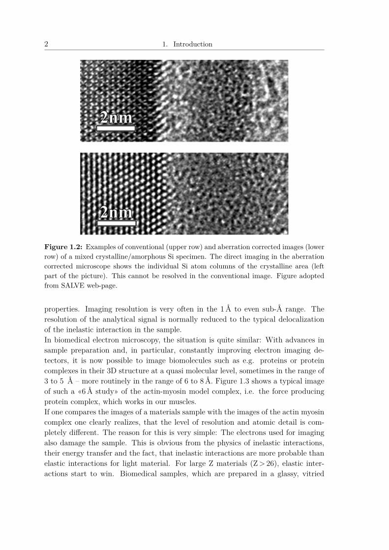
Figure 1.2: Examples of conventional (upper row) and aberration corrected images (lowerrow) of a mixed crystalline/amorphous Si specimen. The direct imaging in the aberrationcorrected microscope shows the individual Si atom columns of the crystalline area (leftpart of the picture). This cannot be resolved in the conventional image. Figure adoptedfrom SALVE web-page.

properties. Imaging resolution is very often in the 1Å to even sub-Å range. Theresolution of the analytical signal is normally reduced to the typical delocalizationof the inelastic interaction in the sample.In biomedical electron microscopy, the situation is quite similar: With advances insample preparation and, in particular, constantly improving electron imaging de-tectors, it is now possible to image biomolecules such as e.g. proteins or proteincomplexes in their 3D structure at a quasi molecular level, sometimes in the range of3 to 5 Å – more routinely in the range of 6 to 8Å. Figure 1.3 shows a typical imageof such a «6Å study» of the actin-myosin model complex, i.e. the force producingprotein complex, which works in our muscles.If one compares the images of a materials sample with the images of the actin myosincomplex one clearly realizes, that the level of resolution and atomic detail is com-pletely different. The reason for this is very simple: The electrons used for imagingalso damage the sample. This is obvious from the physics of inelastic interactions,their energy transfer and the fact, that inelastic interactions are more probable thanelastic interactions for light material. For large Z materials (Z> 26), elastic inter-actions start to win. Biomedical samples, which are prepared in a glassy, vitried

3

Figure 1.3: (A) Images acquired by transmission electron cryo microscopy of F-actin dec-orated with myosin Va motor domains with truncated lever arm, in nucleotide-free Rigorstate. The defocus value is 1.7µm and 5µm for the insert, respectively. (B) The recon-structed density map of the nucleotide-free complex shows the typical helical symmetry ofthe filamentous actin-backbone. Shown are six actin molecules in their ribbon represen-tation (light yellow) and four myosin motor domains (blue). Images from our own paper[?].

aqueous buffer layer of about 50 to 100 nm thickness, are simply «boiled away» byour electron beams. Thus, images have to be taken at lower magnication and lowerelectron dose, which decreases resolution and increases noise.

What will you learn from this experiment?

As you might expect, TEMs which deliver sub-Å resolution or allow the imaging ofa frozen sample at liquid nitrogen temperature are very specialized, expensive, andmost of the time used for our research. A microscope – as small as the one used herein our practical course – will not have all this expensive instrumentation, but willget you acquainted with some very important physical facts, which we in our dailyresearch still have to be aware of. Familiar topics in this respect are the optimal opti-cal alignment of an imaging system in particle optics, basic imaging properties whenworking with a particle beam, the recording of an image and basic image processingsteps. Also, electron diffraction experiments can be performed with our microscope,and very fundamental experiments to test the coherence of an electron beam andhow it can be inuenced by different beam forming parameters. In the end you shouldhave a first feeling – and also the physical basis for it – what it takes to set up amicroscope optimally and how to tune it for highest performance. One of the «holygrails» of transmission electron microscopy, the Contrast-Transfer-Function (CTF),should then be something, which has lost its legendary aura. While we provide a

4 1. Introduction

guideline for experiments with our samples (which we provide as well), we also willgive you samples for «free microscopy». This will be tissue samples from biologicalspecimens, plant root or mouse muscle prepared with different protocols. Besidesall the proposed experiments, documentation, suggested reading, and discussion, wewould like to encourage you to simply «play around» with these samples – followingthe rule that «one can see a lot just by looking». To make this worthwhile – however– we will discuss your images (and your documentation of this free microscopy) withyou and also explain a bit of the biology of the samples.

2. Outline of Experiments

2.1 Day 1

Basic operation and alignment of the transmission electron microscope(TEM)

• Get to know the lens system of the microscope.

• Align the microscope.

• Introduce a sample (holey carbon film) into the beam path and judge the imagequality.

• Acquire images of the holey carbon film.

• Test the effects of astigmatism and over/under focus on images of holes in thefilm.

• Use Fresnel diffraction to investigate the effect coherent illumination has onyour image.

2.2 Day 2

Diffraction Experiments

• Operate the TEM in diffraction mode.

• Understand the formation of diffraction patterns and which information theyprovide about the sample.

• Acquire diffraction patterns of thin films (Au and Au/Pd or Pt/Pd).

• Calibrate the camera length of the microscope using the diffraction pattern ofAu.

Basic Principles of Bright-Field and Dark-Field Microscopy

• Understand imaging in the TEM using a MgO sample.

5

6 2. Outline of Experiments

• Acquire bright- and dark-field images on basis of the according diffraction pat-tern of MgO.

2.3 Day 3

Bright-Field Imaging and Effects of the Contrast-Transfer-Function (CTF)

• Calibrate all (possible) magnification settings using a so called „cross grating“.Also use the latex beads to check your calibration. Discuss errors.

• Measure and use the periodicity of a catalase crystal to calibrate higher mag-nifications.

• Acquire a defocus series of a catalase crystal to understand the effect the Con-trast transfer function has on the image.

• Free microscopy (optional).

3. Course Preparatiom

Work on the following tasks and be prepared to discuss them over the course of thethree days.

3.1 The imaging system of a TEM

The beam paths in electron optics can be drawn analogous to light optics. Chapters6 and 9 of [Wil09] may help you working on the following tasks.

1. Name reasons, why we are using microscopes.

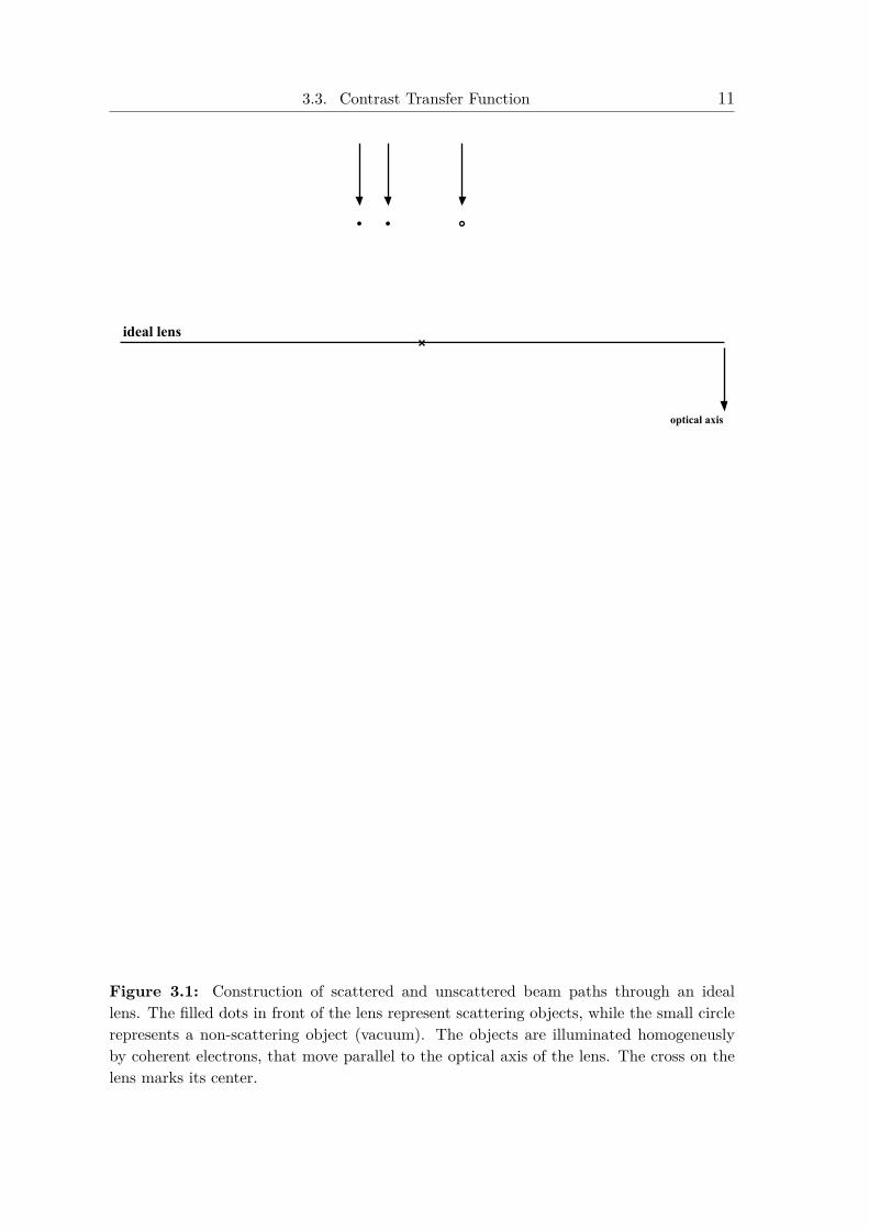
2. Consider two scattering points and one non-scattering point (vacuum) locatedin front of an ideal lens as depicted in figure 3.1 at the end of this section. Youcan use the figure for the following constructions.

• Define the image plane of the lens at an arbitrary, but reasonable placebehind the lens (arbitrary magnification).

• Construct the image of the given objects by using the centre of the lens andthe previous defined image plane. You may benefit from your knowledgeof optical geometry.

• Assume that all electrons (scattered and non-scattered) passing a pointare moving through the according image point in the image plane as well.With this construct the beam paths of non-scattered (0 ◦) and scattered(α) electrons at the following angles α in different colors: 40 ◦, 20 ◦, −20 ◦,−40 ◦

• Mark characteristic points and planes on basis of your constructions andexplain, why they are characteristic.

• Mark in the same figure the location of the following apertures and explaintheir purpose.

– Condenser aperture (CA)– Objective aperture (OA)– Selected-area aperture (SA)

3. Explain the purpouse of the following parts in a basic TEM setup: Condenser,Objective, Projective.

7

8 3. Course Preparatiom

4. You will have to calibrate all magnifications of the microscope in real space andfourier space of an image showing a standard sample. One calibration methodis described in Chapter 9 of [Wil09] (p. 164f).

• Download the image «Calibration.tif» from the link showing an image ofa standard specimen - so called «cross grating» (2160 lines/mm) - withlatex beads on it (black dots with ∅ 0.261µm).

• Open the image in an image program (e.g. Fiji) and get an idea, how tomeasure lengths and intensity profiles with this program. You will needthat for data analysis later on. Helpful features of Fiji can be found inappendix B.

• Find out what measurements need to be done in real space and in thefourier transformation of the image (distance real, diameter latex beads,distance FFT) to calculate the pixel size in the image.

• Argue, why the magnification is calibrated, if you know the pixel size ofall magnification settings and estimate the error you would expect fromyour measurements.

3.2 Diffraction and Bright- and Darkfield-Imaging

Chapters 11 and 12 of [Wil09] may help you working on the following tasks.

1. Explain «contrast».

2. Explain the difference between the following contrast mechanisms and namethe ones used for imaging in a conventional TEM.

• absorption-contrast

• aperture-contrast

• phase-contrast

• filter-contrast

3. Write down the «Bragg condition» and explain, what kind of diffraction patternyou would expect from a single crystal.

4. Write down «Vegard’s law» and calculate the lattice parameter for Pt/Pd andAu/Pd (each 80/20). Estimate, which differences you would expect in thediffraction patterns of Au and Au/Pd or Au and Pt/Pd.

3.3. Contrast Transfer Function 9

5. You will have to calibrate the camera length of the microscope. As for theprevious calibration a suitable method is described in Chapter 9 of [Wil09](p. 165f).

• Download the image «DiffCalib.tif» from the link. This is an image stackcontaining 8 images of a polycrystalline gold diffraction pattern.• Open the image stack in an image program (e.g. Fiji) and use the «Z-

Project» function of Fiji (see appendix B) since this will help you topresent your data later on.• Use the «Radial Profile» function in Fiji to calibrate the camera length.

Estimate the error, you would expect from your measurements.

3.3 Contrast Transfer Function

Sections 6.5 and 28.7 of [Wil09] may help you working on the following tasks.

1. Name possible lens aberrations and how they can be compensated.

2. Explain «Scherzer-Focus» and what it is used for.

3.3. Contrast Transfer Function 11

optical axis

ideal lens

Figure 3.1: Construction of scattered and unscattered beam paths through an ideallens. The filled dots in front of the lens represent scattering objects, while the small circlerepresents a non-scattering object (vacuum). The objects are illuminated homogeneuslyby coherent electrons, that move parallel to the optical axis of the lens. The cross on thelens marks its center.

4. Experimental Procedure

Always make notes of the imaging conditions at which you acquire data/images.Since you want comparable data or be able to reproduce it in the future, this is avery important experimental practice. From the given link you can downloada spreadsheet template, where you can enter all important parameters.

4.1 Day 1

4.1.1 Get to know the microscope

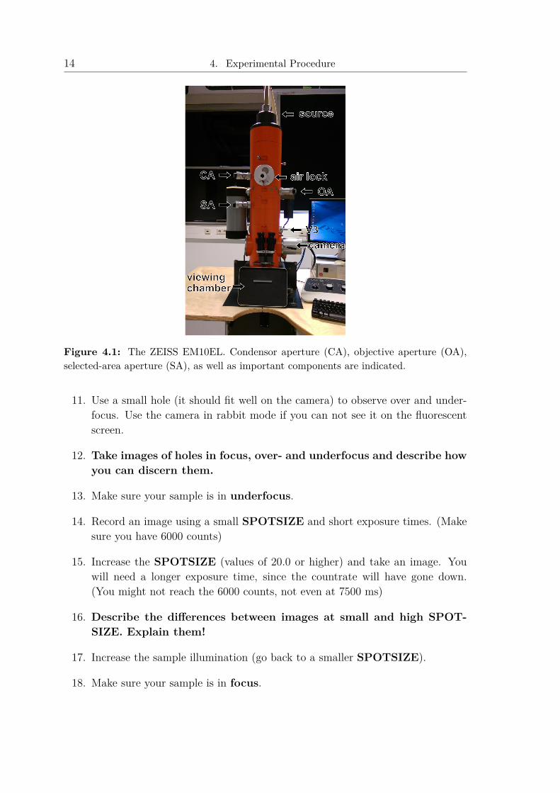
All important components (apertures, valve V3,...) and knobs are indicated in thefigures 4.1 and 4.2.

1. Turn on the microscope as described in the according section in the «AlignmentProcedure EM109EL» document.

2. You will be measuring at 80 kV acceleration voltage and No. «2» emissionsettings in the software (around 5 to 6 µA emission current) unless otherwisestated.

3. Use the «Alignment Procedure» to align the microscope and record flat-field/background images for the camera.

4. Insert the holey carbon film sample. Go to a sample area containing holes.

5. Go to a magnification of about 20 kx.

6. Toggle the FOCUS wheel.

7. Describe how to determine that your sample is in focus.

8. Go to diffraction mode (DIFF). Insert and center the first Objective Aper-ture. The handling of the aperture knobs is described in figure 4.3.

9. Go to image mode (DIFF). Do you see a difference in your image? Takeimages showing these differences and explain it.

10. Describe what happens when you switch to different magnifications.Explain the rotation of the image.

13

14 4. Experimental Procedure

Figure 4.1: The ZEISS EM10EL. Condensor aperture (CA), objective aperture (OA),selected-area aperture (SA), as well as important components are indicated.

11. Use a small hole (it should fit well on the camera) to observe over and under-focus. Use the camera in rabbit mode if you can not see it on the fluorescentscreen.

12. Take images of holes in focus, over- and underfocus and describe howyou can discern them.

13. Make sure your sample is in underfocus.

14. Record an image using a small SPOTSIZE and short exposure times. (Makesure you have 6000 counts)

15. Increase the SPOTSIZE (values of 20.0 or higher) and take an image. Youwill need a longer exposure time, since the countrate will have gone down.(You might not reach the 6000 counts, not even at 7500 ms)

16. Describe the differences between images at small and high SPOT-SIZE. Explain them!

17. Increase the sample illumination (go back to a smaller SPOTSIZE).

18. Make sure your sample is in focus.

4.2. Day 2 15

Figure 4.2: Control panel for the ZEISS EM10EL.

19. Set the Objective Stigmator (OBJ STIG) to maximum, which induces astig-matism to the image. Describe how the image changed.

20. Record an image (6000 counts) of a hole, which shows astigmaticcharacteristics.

21. Reset the Objective Stigmator (OBJ STIG - RECALL).

22. You should have recorded at least 6 images. Make sure, you saved them.

23. When done. Remove all apertures. Close V3.

24. Remove the camera from the beam path.

25. Remove the sample from the beam path.

26. Turn off the filament and then the high tension.

27. When you have saved all your images, shut down the camera computer.

28. Turn off the microscope in the microscope software. (Make sure the cameracomputer has shut down completely.)

29. Shut down the microscope computer.

30. Finish Day 1.


Figure 4.3: (Objective) aperture drive. Turning 1 will let you insert or remove thedifferent sized apertures. The black knobs (2 and 3) let you move the aperture in x and ydirection.

4.2 Day 2

4.2.1 Diffraction Experiments

1. Turn on the Microscope. (80 kV, 5 to 6µA)


3. Make sure no objective aperture is inserted.

4. Change the Holey Carbon film with the Au sample and insert the sampleholder into the microscope. If neccessary ask the instructor to help you.

5. Go to an area containing the sample film.

6. Use a Magnification of 20 kx.

7. Go to diffraction mode (DIFF).

8. Describe what you see.

9. Go back to image mode (DIFF).

10. Insert and center the smallest selected-area aperture (SA).

11. Go back to diffraction mode (DIFF).

4.2. Day 2 17

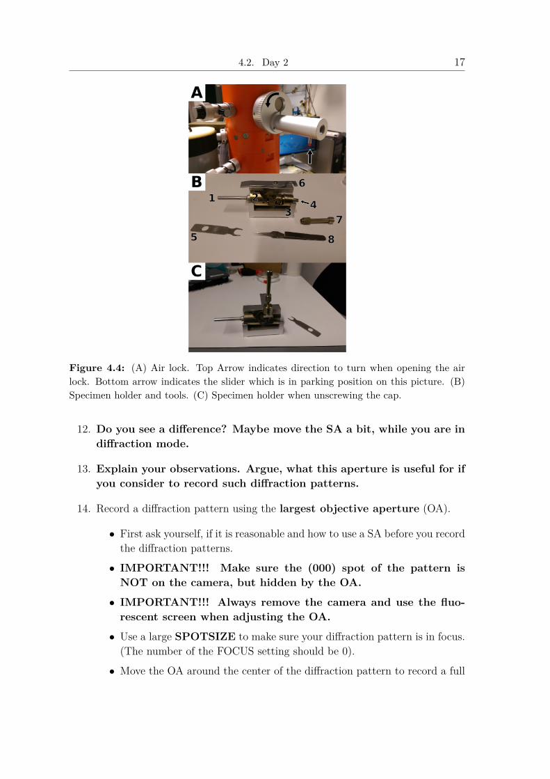
Figure 4.4: (A) Air lock. Top Arrow indicates direction to turn when opening the airlock. Bottom arrow indicates the slider which is in parking position on this picture. (B)Specimen holder and tools. (C) Specimen holder when unscrewing the cap.

12. Do you see a difference? Maybe move the SA a bit, while you are indiffraction mode.

13. Explain your observations. Argue, what this aperture is useful for ifyou consider to record such diffraction patterns.

14. Record a diffraction pattern using the largest objective aperture (OA).

• First ask yourself, if it is reasonable and how to use a SA before you recordthe diffraction patterns.

• IMPORTANT!!! Make sure the (000) spot of the pattern isNOT on the camera, but hidden by the OA.

• IMPORTANT!!! Always remove the camera and use the fluo-rescent screen when adjusting the OA.

• Use a large SPOTSIZE to make sure your diffraction pattern is in focus.(The number of the FOCUS setting should be 0).

• Move the OA around the center of the diffraction pattern to record a full


diffraction pattern of Au at 150mm Camera Length (CL). (You will needabout 4 to 8 images).

• Later on in your analysis you will load them as an „image sequence“ intoFiji.

• Record a second diffraction pattern of Au at 250mm Camera Length.

• Center the OA around the center spot to increase contrast in your image.

• Switch to image mode (DIFF).

• Go to highest magnification.

• Try to record an image of the Au crystals. Use the «rabbit» mode tofocus your image.

15. Use the diffraction patterns of Au later to calibrate the two Camera Lengthsof the microscope.

16. When done. Remove all apertures and close V3. Turn off the filament.

17. Switch the sample. Choose either Au/Pd or Pd/Pt.

18. Follow the steps in 14 to record a full diffraction pattern and images of thenew sample.

19. Do you see a difference between the diffraction patterns of Au and the sampleyou chose? If so, explain where it comes from.

20. Is there a difference between the images of the samples?

21. When done, you should have recorded a set to create a full diffrac-tion pattern for Au and Au/Pd or Pt/Pd at camera lengths 150mmand 250mm, as well as images of the crystalline film at highest mag-nification.

22. Remove all apertures, close V3 and turn off the filament.

23. Remove the sample holder.

4.2.2 Bright-/Dark-Field Imaging

1. Insert the MgO sample.

2. Use the «Alignment Procedure» to make sure the beam is aligned.

3. Find a sample area.

4.2. Day 2 19

4. Toggle magnification, focus and spotsize to investigate your sample. Describe,what you see.

5. Go to 20 kx or 30 kx.

6. Insert and center the SA and go to diffraction mode (DIFF).

7. Insert and center the small OA (2nd aperture position).

8. Go to image mode (DIFF) and acquire a so called bright-field (BF) image.Make sure it is in focus (use the «rabbit mode» if necessary).

9. In diffraction mode, center the OA around a diffracted beam to acquirea dark-field (DF) image.

10. Go to image mode and acquire a DF image.

11. Do this for several diffraction spots and explain your observation.

12. In the same way describe and explain your observation, if you takeDF images of two opposing diffraction spots (Friedel pair).

13. Choose different sample positions and diffraction spots to see what you can dowith DF imaging. Feel free to go to higher magnifications.

14. You should have acquired at least one BF image of a sample area anda few DF images from opposing and non-opposing diffraction spots.Remove all apertures.

15. Remove the sample and the camera from the beam path.

16. Close V3.

17. Turn off the filament and afterwards the high tension.




21. Finish Day 2.


4.3 Day 3

4.3.1 Calibration with Cross-Grating

1. Turn on the Microscope.


3. Insert the sample holder containing the cross-grating replica.

4. You should see a cross-grating (2160 lines/mm) with latex spheres (∅ 0.261µm).

5. Take images of the cross-grating at each (high mag) magnification setting(3 kx to 250 kx).

• Make sure the sample is in focus.

• At higher magnifications, make sure to get as many straight lines as possi-ble on the camera (use the «rabbit mode» if necessary). Sometimes thereare irregularities in the cross-grating that will make it hard to get a goodcalibration. Also try to get good images of the spheres to check yourcalibration.

• You will have to adjust SPOTSIZE and exposure time as you go tohigher magnifications.

6. Talk with the instructor how to measure the pixel size from the real space andfrom the FFT of the image using Fiji.

7. Describe the differences in the FFT at lower and higher magnifica-tion.

8. You should now have at least one image of the cross-grating and/or latexspheres for each (possible) magnification.

9. Remove the sample and the camera from the beam path.

10. Close V3.

11. Turn off the filament and afterwards the high tension.

12. Remove all apertures and close V3.

13. Remove the sample holder with the cross-grating replica.

4.3. Day 3 21

4.3.2 Calibration with Catalase Crystals

1. Insert the sample holder containing the catalase sample.

2. While you change the sample, describe the effect of negative stain.

3. Once the filament has ramped up, change the Emission setting to «3» in thesoftware. You should now have a much larger emission current.

4. Use the «Alignment Procedure» to align the microscope and record flat-field/background images for the camera. If you change the emission new flat-field/background images are needed.

5. Investigate the sample and describe what you see.

6. Use the OA to increase the contrast.

7. Use the support film to correct the Objective Astigmatism (Obj Stig)at high magnification for best results. Make sure you have a good flat-fieldcorrection. You might need to use a higher spotsize, longer exposure times anda sufficient high defocus to see the so called «Thon Rings».

8. Talk with the instructor about the origin of these Thon Rings.

9. Find a catalase crystal.

10. Bring the catalase crystal into focus. (use the «rabbit mode» if neccessary).

11. Start at a magnification where you first see the catalase crystal spacings (notethe FFT). Record images of the catalase crystal spacings. Do this forall higher magnification settings.

12. You will need to use the catalase to calibrate the higher magnifications sincethe lines of the cross-grating are too large.

13. When done, you should have images of the catalase crystal for each of themagnification settings in which you can see the spacings.

14. Use these images to calibrate the higher magnification settings of the micro-scope from real space and from the FFT of the images.


4.3.3 Contrast Transfer Function

1. Choose a (high) magnification where you can see the «Thon Rings» and thecrystal spacings in the FFT as well.

2. Change the focus to higher defocus and watch the crystal spacings. Describewhat you see.

3. Record a so called defocus series

• Start at focus and go to higher underfocus (defocus).• Watch the crystal spacings until you realize a changes in the image.• Observe the FFT (also called diffratogram or power spectrum) closely and

describe what happens there as well while changing the focus.• Take images of your observations.

4. Remove all apertures and close V3. Turn off the filament.

5. Remove the sample holder.

4.3.4 Free Microscopy

1. Ask the instructor to give you a sample for free microscopy. This can forexample be a piece of mouse muscle or some cress root. Insert it into themicroscope.

2. Use the «Alignment Procedure» (steps 1 to 3) to make sure the beam is aligned.Go back to Emission Setting No. «2». (5 to 6µA)

3. Use your newly acquired «microscopy skills» to investigate the sample, improvecontrast and record some images.

4. When done, remove all apertures and close V3.

5. Turn off the filament and then the high tension.




9. Make sure you ask the instructor about anything that was unclear.

10. Finish Day 3.

5. Expected Documentation of the Experiments

Important! All real space images should contain a scalebar. In order to do thisyou need to calculate the pixelsize for the specific image first. Afterwards you canadd a scalebar using Fiji (B).Indicate on your diffraction patterns the used camera length.

5.1 Day 1

• Explanation of the lens system and basic setup of a TEM.

• Short explanation about the formation of Fresnel Fringes in your images.

• Explanation of over- and underfocus using images of a holey carbon film andhow the contrast of an image in focus can be increased.

• Demonstrating the effect of astigmatism in an image you recorded.

• Showing, how coherence affects the image quality by judging the visibility ofFresnel diffraction patterns inside a hole in a carbon film.

5.2 Day 2

• Explain diffraction. Take the Bragg and Laue condition into account and show,how they are related.

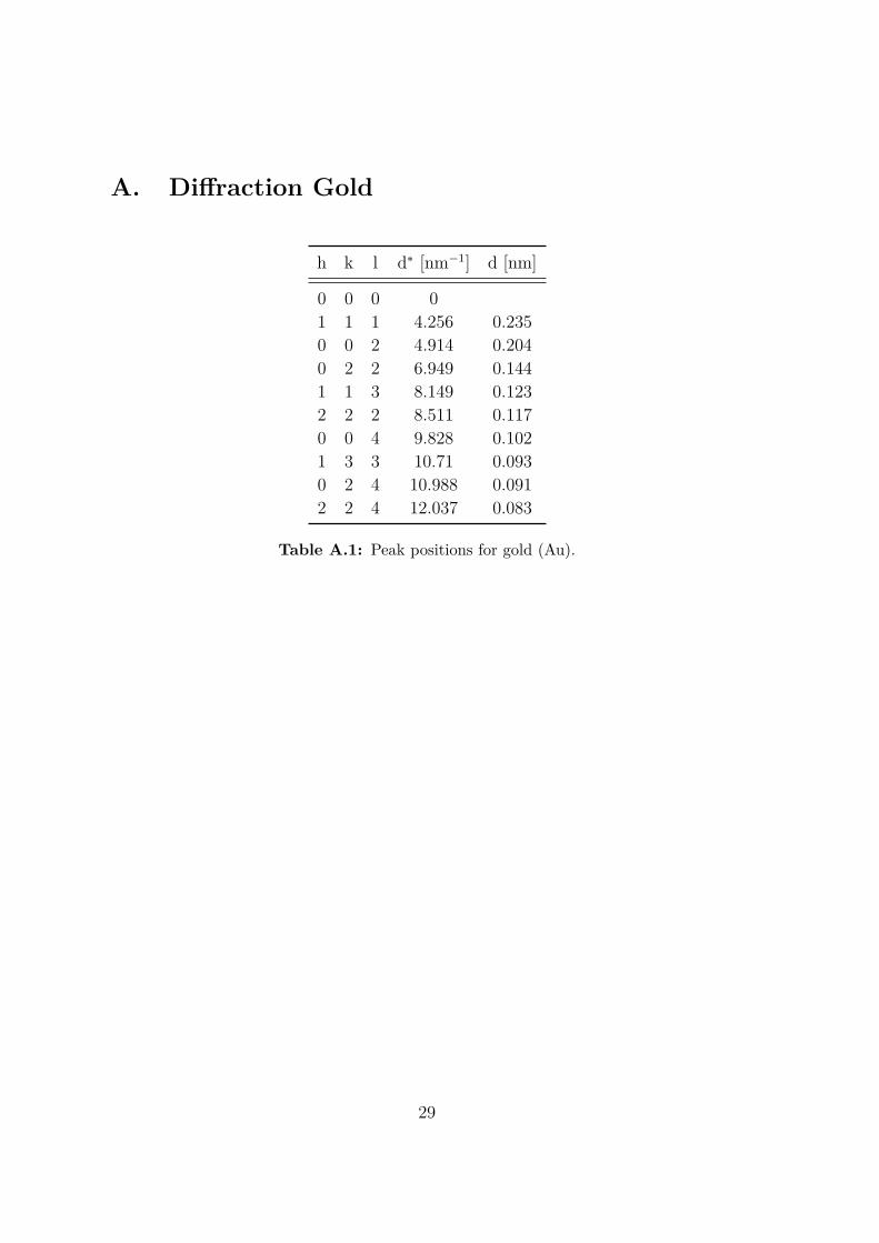
• Index the diffraction pattern of gold. (See the table A.1 in the appendix.)

• Calibrate the camera lengths at 150mm and 250mm.

• Analyze the diffraction patterns of Pt/Pd or Au/Pd at the camera lengths150mm and 250mm respectively. Don’t forget to indicate the errors risingfrom your measurements.

• Calculate the lattice parameter for the sample you chose using Vegard’s lawand compare them with your measurements (Use Bragg’s law).

• Discuss possible errors.

• Explanation of bright-field/dark-field images from the MgO sample.

23

24 5. Expected Documentation of the Experiments

5.3 Day 3

• Create a calibration table for all magnification settings. Indicate the methodsand the specimen you used for the calibration.

• Plot the calculated pixel size for each calibration method along with the realmagnification. Compare it to the nominal magnification of the microscope.

• Discuss possible errors and show, why you need different specimens for cali-brating all magnification settings.

• Show images of Catalase, which is a protein crystal prepared as negative stainsample, and explain «negative stain».

• Show the «Thon Rings» in the power spectrum of an catalase image and howthey change at different imaging conditions.

• Show the effect the Contrast Transfer Function has on the image and try togive an explanation of it (No formulas!).

• Images of «free microscopy» with a description, what can be seen there.

Bibliography

[Ern10] R. Erni. Aberration-corrected imaging in transmission electron microscopy:an introduction (ICP/Imperial College Press; Distributed by World ScienticPub. Co, London : Singapore; Hackensack). 2010.

[Hai98] M. Haider, H. Rose, S. Uhlemann, E. Schwan, B. Kabius undK. Urban. Aspherical-aberration-corrected 200 kV transmission electronmicroscope. Ultramicroscopy, 75, 1, 53–60. 1998.

[Rei08] L. Reimer und H. Kohl. Transmission Electron Microscopy, volume 36of Springer Series in Optical Sciences (Springer New York). 2008.

[Rod18] J. Rodenburg. The beginner’s guide to transmission electron microscopy.URL http://www.rodenburg.org/guide/index.html. 2018.

[Wil09] D. B. Williams und C. B. Carter. Transmission Electron Microscopy:A Textbook for Materials Science (Springer Science & Business Media).2009.

25

26 Bibliography

Appendices

27

A. Diffraction Gold

h k l d∗ [nm−1] d [nm]

0 0 0 01 1 1 4.256 0.2350 0 2 4.914 0.2040 2 2 6.949 0.1441 1 3 8.149 0.1232 2 2 8.511 0.1170 0 4 9.828 0.1021 3 3 10.71 0.0930 2 4 10.988 0.0912 2 4 12.037 0.083

Table A.1: Peak positions for gold (Au).

29

30 A. Diffraction Gold

B. Helpful Features in Fiji

Fiji (Fiji is just ImageJ) is an opensource software for scientific image processing.You can use it to calibrate and analyze electron microscopy images. Fiji (includingthe Raial Profile Plugin) is installed on the CIP-Pool computers.Download sources and further information can be found on the internet:

• Fiji can be downloaded here for all common used operating systems:

http://imagej.net/Fiji/Downloads

• The Radial Prole Plugin here:

https://imagej.nih.gov/ij/plugins/radial-prole.html

• An extensive documentation for ImageJ in general can be found under:

https://imagej.nih.gov/ij/docs/guide/index.html

B.1 Opening images and scalebars

Single images can be open by drag and drop. You can open several images as onestack under:

File → Import → Image Sequence.

Fiji cannot read any calibration done by this camera software. Reset the image sizeto pixels for each image under:

Analyze → Set Scale → button «click to remove scale»

Here you can enter the results from your calibration as well, by entering the calculatedpixel size in nm, once you know it. A scalebar can be added to your image under:

Analyze → Tools → Scale Bar

B.2 Adjusting Brightness and Contrast

The images you acquired during the experiment will be 16-bit greyscale. Some-times, especially at higher magnications, the intensity during acquisition was low.

31

32 B. Helpful Features in Fiji

This might cause your image to appear black at first, since Fiji will use the whole(gray scale) histogram to display the image. You can adjust the histogram under:

Image → Adjust → Brightness/Contrast

Using the shortcut «Ctrl + C» works even quicker. Pressing the «Auto»-button inthe window often yields to a nice view. After you have adjusted this to your liking,you can change the type of your image to 8-bit (Image -Type -8-bit). Fiji will thendiscard the information that you did not select in the histogram. Changing yourimages to 8-bit is sometimes helpful, since they will then take up less disk space.

B.3 Fast Fourier Transforms

If you need to calculate the FFT of an image (e.g. for calibration), this can be doneunder:

Process → FFT → FFT

This works even for a selected area of your image. When hovering the mouse pointerover a pixel of interest in the FFT, Fiji will display its position in the FFT and therespective distance in the real image. This can help you calibrate the magnication.Have your instructor show this to you.

B.4 Image Stacks

Image stacks can be created from sequential images, while the slider in the windowof an image stack represents the «Z-axis» of the stack. You can create a projectionof all images in the stack by using:

Image → Stacks → Z-Project

When putting together the recorded partial diffraction patterns, choosing «Max In-tensity» will let you create a single image containing the brightest parts of each singleimage. This is useful for creating a nice full diffraction pattern from your partialones.

B.5. Radial and Line Profile 33

B.5 Radial and Line Profile

For your calibration you need to meassure lengths in your images (e.g. cross-grating).For proper measurements (including error estimation) you should use «Line Profiles».Draw a line across the image using the «line tool». Double clicking the tool buttonlets you change the width of the line. You get a line profile under:

Analyze → Plot Profile

Clicking the «List» button in the profile window will give you the x and y coordinates.You can export them (e.g. as .txt-file) and plot/analyze the profile in a softwareof your choice. The «live» button in the profile window allows you rearrange thedrawn line in the image, while keeping the plot profile updated in real time. This isespecially helpful for the radial profile.

The radial profile is similar to the plot profile. It measures the mean intensity ofconcentric circles as a function of the radius. Once you have installed the «RadialProfile» plugin, fit a circle to the data (e.g. of diffraction patterns). Make sure youpress «Shift» so your circle becomes round and not elliptic. It is important that theplugin knows where the center of the circle is located since this will define the zeroposition of the radial profile. Be precise with fitting the circle. Otherwise the errorof the measurement increases. Make use of the «live» button to optimize the circleposition.

34 B. Helpful Features in Fiji

C. Provided Samples

• Holey carbon film

• Gold (Au)

• Gold/Palladium (Au/Pd 80:20)

• Platinum/Palladium (Pt/Pd 80:20)

• Magnesium oxide crystals

• Cross-grating calibration sample with latex spheres (2160 lines/mm, ∅ 0.261µm)

• Bovine catalase

• Samples for «free microscopy», will vary from group to group, usually samplesof plant root material and/or tissue samples, e.g. from mouse muscle.

35

f90 - transmission electron microscopy - physikalisches ... · transmission electron microscopy,...

Documents