Correction

EVOLUTIONCorrection for “Extremely high genetic diversity in a single tumorpoints to prevalence of non-Darwinian cell evolution,” byShaoping Ling, Zheng Hu, Zuyu Yang, Fang Yang, Yawei Li, PeiLin, Ke Chen, Lili Dong, Lihua Cao, Yong Tao, Lingtong Hao,Qingjian Chen, Qiang Gong, Dafei Wu, Wenjie Li, WenmingZhao, Xiuyun Tian, Chunyi Hao, Eric A. Hungate, Daniel V. T.Catenacci, Richard R. Hudson, Wen-Hsiung Li, Xuemei Lu, andChung-I Wu, which appeared in issue 47, November 24, 2015, ofProc Natl Acad Sci USA (112:E6496–E6505; first published No-vember 11, 2015; 10.1073/pnas.1519556112).The authors note that Chunyi Hao should be listed as an addi-

tional corresponding author. The corrected correspondence foot-note appears below. The online version has been corrected.

2To whom correspondence may be addressed. Email: ciwu@uchicago.edu,whli@gate.sinica.edu.tw, luxm@big.ac.cn, or haochunyi@bjmu.edu.cn.

www.pnas.org/cgi/doi/10.1073/pnas.1600151113

www.pnas.org PNAS | February 2, 2016 | vol. 113 | no. 5 | E663

CORR

ECTION

Extremely high genetic diversity in a single tumorpoints to prevalence of non-Darwinian cell evolutionShaoping Linga,1, Zheng Hua,1, Zuyu Yanga,1, Fang Yanga,1, Yawei Lia, Pei Linb, Ke Chena, Lili Donga, Lihua Caoa,Yong Taoa, Lingtong Haoa, Qingjian Chenb, Qiang Gonga, Dafei Wua, Wenjie Lia, Wenming Zhaoa, Xiuyun Tianc,Chunyi Haoc,2, Eric A. Hungated, Daniel V. T. Catenaccie, Richard R. Hudsonf, Wen-Hsiung Lig,2, Xuemei Lua,2, and Chung-I Wua,b,f,2

aKey Laboratory of Genomics and Precision Medicine, China Gastrointestinal Cancer Research Center, Beijing Institute of Genomics, Chinese Academy ofSciences, University of Chinese Academy of Sciences, Beijing 100101, People’s Republic of China; bState Key Laboratory of Biocontrol, College of Ecologyand Evolution, Sun Yat-Sen University, Guangzhou 510275, People’s Republic of China; cKey Laboratory of Carcinogenesis and Translational Research,Peking University Cancer Hospital, Beijing 100142, People’s Republic of China; dDepartment of Pediatrics, University of Chicago, Chicago, IL 60637;eDepartment of Medicine, Section of Hematology/Oncology, University of Chicago, Chicago, IL 60637; fDepartment of Ecology and Evolution, University ofChicago, Chicago, IL 60637; and gBiodiversity Research Center, Academia Sinica, Taipei 11529, Taiwan

Contributed by Wen-Hsiung Li, October 10, 2015 (sent for review September 14, 2015; reviewed by Takashi Gojobori and Jianzhi Zhang)

The prevailing view that the evolution of cells in a tumor is drivenby Darwinian selection has never been rigorously tested. Becauseselection greatly affects the level of intratumor genetic diversity, itis important to assess whether intratumor evolution follows theDarwinian or the non-Darwinian mode of evolution. To providethe statistical power, many regions in a single tumor need to besampled and analyzed much more extensively than has beenattempted in previous intratumor studies. Here, from a hepatocel-lular carcinoma (HCC) tumor, we evaluated multiregional samplesfrom the tumor, using either whole-exome sequencing (WES) (n =23 samples) or genotyping (n = 286) under both the infinite-site andinfinite-allele models of population genetics. In addition to themany single-nucleotide variations (SNVs) present in all samples,there were 35 “polymorphic” SNVs among samples. High geneticdiversity was evident as the 23 WES samples defined 20 unique cellclones. With all 286 samples genotyped, clonal diversity agreed wellwith the non-Darwinian model with no evidence of positive Dar-winian selection. Under the non-Darwinian model, MALL (the num-ber of coding region mutations in the entire tumor) was estimatedto be greater than 100 million in this tumor. DNA sequences reveallocal diversities in small patches of cells and validate the estimation.In contrast, the genetic diversity under a Darwinian model wouldgenerally be orders of magnitude smaller. Because the level of ge-netic diversity will have implications on therapeutic resistance, non-Darwinian evolution should be heeded in cancer treatments evenfor microscopic tumors.

intratumor heterogeneity | genetic diversity | neutral evolution |cancer evolution | natural selection

The level of genetic diversity in a natural population is de-termined by several evolutionary forces, including mutation,

genetic drift, migration, and natural selection (1–3). Tumors can beregarded as asexual populations of cells, so they are subjected tosimilar forces to those of natural populations (4–7). Therefore, thegenetic diversity in tumors of the same patient is informative abouthow various forces drive their evolution. The level of diversity mayalso influence how tumors respond to environmental perturbations,either natural or medical (5–7). In the prevailing view, Darwinianselection for and against new mutations is the main driving force ofintratumor diversity (4, 8–18). Because selection generally reducesgenetic diversity within populations (19–21), studies assumingDarwinian evolution usually described MALL (the total number ofcoding region mutations within the whole tumor) in the range oftens to hundreds of coding mutations (22, 23).Despite its wide acceptance, the Darwinian view has never been

subjected to hypothesis testing, by which the observed diversityis compared with quantitative predictions. This study is to ourknowledge the first one that uses high-density sampling in a singletumor and compares the observations with theoretical predictions.In this test, we consider a null model of non-Darwinian evolution

in which MALL is a function of N (population size), u (mutationrate per generation), and growth parameters. In tumors, N islarge, generally � 106, and u is the mutation rate of the entirefunctional portion of the genome (at the level of 10−2 per celldivision) (18, 24). Hence, the expected genetic diversity oftumors by non-Darwinian evolution would be large, probablyon the order of millions of mutations, most of which are presentat low frequencies (25).We ask whether the observed intratumor genetic diversity can

be largely explained by non-Darwinian forces and we invokepositive selection only when the null model of non-Darwinianevolution is rejected. There was a controversy in molecularevolution generally known as the neutralism–selectionism debate(1, 26, 27). In the postdebate modern view, genetic polymor-phisms in natural populations are largely consistent with the non-Darwinian model (1–3, 26–28). There are further reasons toquestion the efficacy of selection within populations of cells thatmake up tumors (Discussion). For instance, although selectionagainst nonsynonymous mutations is nearly universal in natural

Significance

A tumor comprising many cells can be compared to a naturalpopulation with many individuals. The amount of genetic di-versity reflects how it has evolved and can influence its fu-ture evolution. We evaluated a single tumor by sequencing orgenotyping nearly 300 regions from the tumor. When the datawere analyzed by modern population genetic theory, we esti-mated more than 100 million coding region mutations in this un-exceptional tumor. The extreme genetic diversity implies evo-lution under the non-Darwinian mode. In contrast, under theprevailing view of Darwinian selection, the genetic diversitywould be orders of magnitude lower. Because genetic diversityaccrues rapidly, a high probability of drug resistance should beheeded, even in the treatment of microscopic tumors.

Author contributions: X.L. and C.-I.W. designed research; Z.Y., F.Y., K.C., D.W., W.L., andW.Z. performed experiments, S.L., Z.H., Z.Y, F.Y., Y.L., P.L., L.D., L.C., Y.T., L.H., Q.C., and Q.G.analyzed data; S.L., Z.H., Y.L., P.L., E.A.H., D.V.T.C., R.R.H., and C.-I.W. contributed to thetheory; X.T. and C.H. provided clinical samples; S.L., L.D., and L.C. contributed new analytictools; and S.L., Z.H., W.-H.L., X.L., and C.-I.W. wrote the paper.

Reviewers: T.G., King Abdullah University of Sciences and Technology; and J.Z., Universityof Michigan.

The authors declare no conflict of interest.

Data deposition: The sequence data reported in this paper have been deposited in thegenome sequence archive of Beijing Institute of Genomics, Chinese Academy of Sciences,gsa.big.ac.cn (accession no. PRJCA000091).1S.L., Z.H., Z.Y., and F.Y. contributed equally to this work.2To whom correspondence may be addressed. Email: ciwu@uchicago.edu, whli@gate.sinica.edu.tw, luxm@big.ac.cn, or haochunyi@bjmu.edu.cn.

This article contains supporting information online at www.pnas.org/lookup/suppl/doi:10.1073/pnas.1519556112/-/DCSupplemental.

E6496–E6505 | PNAS | Published online November 11, 2015 www.pnas.org/cgi/doi/10.1073/pnas.1519556112

species (1, 3, 27), selection against such mutations in tumors isnot apparently stronger than against synonymous ones (29).In the recent literature, there has been increasingly more at-

tention on assessing the non-Darwinian model of tumor evolutionvs. the prevailing Darwinian view (30, 31). Tao et al. (31) studied12 cases of multitumor hepatocellular carcinomas (HCCs) andconcluded that competition often occurs between tumors largeenough to be visible. In contrast, the genetic diversity containedwithin the same tumor does not deviate from the predictions ofthe non-Darwinian model. A caveat is that whereas the number ofpopulation samples used in testing Darwinian selection in naturalpopulations is often in the hundreds, the sample number rarelyexceeds 10 in intratumor studies (12, 13, 15–18, 30, 31). Therefore,the power to reject the null model in tumor studies might havebeen too low. Clearly, there is a need to sample a large number ofregions in one single tumor. In this study we sampled close to 300regions to examine the spatial distribution of single-nucleotidevariants and to estimate the amount of genetic diversity in thetumor. We used these data to give a rigorous test of the null hy-pothesis of non-Darwinian evolution.

ResultsSampling, Sequencing/Genotyping, andMutation Calling.The honeycomb-like microdissections yielded 286 tumor samples on a plane of asingle HCC tumor (Materials and Methods, section 1), each samplebeing a cylinder of 0.5 mm in diameter and 1 mm in height (Fig.1A and Fig. S1). A sample contained, on average, 20,000 cells (Fig.S2 and Materials and Methods, section 2) and permitted precisedelineation of clones. Fig. 1A displays the spatial distribution of the286 tumor samples, which were evenly distributed among the fourquadrants of the tumor slice, labeled A–D clockwise. The 23 se-quenced samples (red color in Fig. 1A) were also evenly distributed,with 12 on the periphery of the tumor and 11 in the interior.For sequencing, the average read depth was 74.4× per sample

(Dataset S1), yielding a total of >1,700× for the plane of Fig. 1A(SI Materials and Methods). With the additional genotyping over286 samples, the coverage is to our knowledge the highest evercarried out on a single tumor. The average sample purity is 85%as described in the legend of Fig. 1A (Materials and Methods,section 3). In total, we found 269 single-nucleotide variations(SNVs) in coding regions or at splice sites (Materials and Methods,

Fig. 1. Sampling scheme and clonal genealogy of HCC-15. (A) Samples were taken from a 1-mm-thick slice cut through the middle of a HCC tumor, 3.5 cm indiameter. Of the 286 samples, 23 were subjected to whole-exome sequencing (red numbers) and the rest (black numbers) were used in genotyping for mutationsdiscovered in sequencing (Materials andMethods, sections 1–5). The numbers correspond with those of Fig. 2. Across the sequenced samples, the average read depthwas 74.4× (Dataset S1). On average, these samples contained 85% cancerous cells estimated by ABSOLUTE (52). This level of purity is consistent with previous reportsregarding hepatic tumor samples (12), especially when the sample volumes are small (∼20,000 cells). Pathology reports, when available for thematchedHCC samples,generally agreed with the purity estimates. (B) All 35 polymorphic nonsynonymous mutations in the sequenced samples are shown in the heat map, which depictsthe observed frequencies (from 0 in white to 1 in yellow) with mutation names at the top of the map. Each row presents the mutations in a sequenced sample. FarRight shows six fixed mutations that are potential drivers. Left shows the genealogy of the 24 samples. Only two clones, indicated by blue bars, are represented bymore than one sample. (C) The genealogy of clones arranged to reflect their spatial relationships. The ancestral clone, Ω, is in the middle and the descendant clonesradiate outward. These clones are arranged on six rings with each outer ring having one more nonsynonymous mutation (indicated) than its interior neighbor. Eachstar symbol represents a singleton clone. (D) The expanded genealogy that includes all 286 samples. The blue stars designate the sequenced samples.

Ling et al. PNAS | Published online November 11, 2015 | E6497

EVOLU

TION

PNASPL

US

sections 4 and 5 and Dataset S2). Due to the dense sampling, SNVsfound in multiple samples are unambiguous by the cross-validationamong samples, using whole-exome sequencing (WES) and/orSequenom. Singleton SNVs (i.e., occurring in only one sample) re-quired additional validations. By Sequenom genotyping, andsometimes Sanger sequencing, all singleton SNVs presented havebeen confirmed to be true positives (Datasets S2 and S3 and Fig.S3). Therefore, the final SNV calls for this study are consideredfree of false positives. Furthermore, given the large number ofsamples, false negatives would likely be negligible.Copy number alterations (CNAs) are another common source

of somatic genomic aberration. We used the program packageCAScnv to call CNAs from our data (Materials and Methods,section 3). On average, each sample contained 23.6 CNAs, dis-tributed among 14 chromosomes (SI Materials and Methods andDataset S4). Because the mechanisms of CNA production are verydifferent from those for SNVs, and because the latter also aremuch easier to ascertain, this study focused on SNVs (Discussion).

Fixed and Polymorphic Somatic Mutations. Somatic mutations dis-covered in the sequenced samples were classified as either fixed orpolymorphic. In this study, the terminology of population geneticsis applied to facilitate theoretical analyses. Fixed mutations werethose present in the entire cancerous cell population but absent inthe noncancerous sample. These mutations must have alreadyoccurred at the onset of tumorigenesis. Polymorphic mutations, onthe other hand, were present in some but not all cancerous sam-ples (Materials and Methods, section 6).Among the 269 SNVs observed in HCC-15, 209 and 35 mutations

were confirmed to be fixed and polymorphic, respectively (DatasetsS2 and S3 and Fig. S4). The remaining 25 mutations, divided into 22possibly fixed and 3 possibly polymorphic SNVs, were not used inthe analysis. The 35 validated polymorphic SNVs would define clonesizes and delineate clonal boundaries according to the genotypes ofthe 286 samples (Materials and Methods, section 7 and Dataset S3).The 209 fixed mutations are divided into 166 protein-altering

mutations (comprising 148 missense, 11 nonsense, and 7 splicingmutations) and 43 synonymous changes. In Materials and Methods,section 8, Fig. S5, and Dataset S5, a list of “driver” genes that aresignificantly more commonly mutated in cancer samples, especiallyin gastrointestinal and HCC tumors [Dataset S6; https://tcga-data.nci.nih.gov/tcga/tcgaHome2.jsp; Schulze et al. (32)], was compiledfrom published data. In reference to this list, we identified 6 pu-tative driver genes among the fixed mutations, which were CCAR1,CPXM2, DNAH7, TMPRSS13, TP53, and TSC1. In contrast,none of the 35 polymorphic mutations is in the driver group.The pathways represented by the fixed and polymorphic mu-tations are also somewhat dissimilar, as shown in Dataset S7.

Clonal Diversity and Genealogy.The 35 validated polymorphic SNVsdelineated 20 cell clones among the 23 sequenced samples. Aclone is defined as a cell population carrying a unique set of so-matic mutations. We denoted Φi as the number of clones thatappeared i times in n samples. The vector of [Φi, i in 1 to n − 1] isthe allele frequency spectrum in population genetics (2, 3). In ourdata, [Φi = 18, 1, 1, 0, 0, 0 . . .; i = 1–22] and n = 23 = 18 × 1 + 1 ×2 + 1 × 3. In other words, 20 (= 18 + 1 + 1) clones consisted of18 singletons, 1 doubleton, and 1 tripleton, which were, respec-tively, cell clones represented by one, two, or three samples. Thesmall number of samples (3 of 23) yielding redundant informa-tion was indicative of the extensive diversity in the coding re-gions of the tumor. In particular, Simpson’s diversity index, H =1 − Σ(Φi/n)

2, was 0.941, indicating that two random sampleswould have a very high probability of being genetically different.The genealogical relationship of the 20 clones is shown in Fig.

1B. The same genealogy with spatial information is given in Fig. 1C,in which clones were shown to emanate from the ancestral Ω clonein the center. For visual clarity, these clones were arranged on fiverings, denoting the number of mutations away from Ω. The 7 directdescendants of Ω, labeled from α to η, all carried 1–2 mutations inaddition to that of the Ω clone. Their descendant clones, eachhaving additional mutations, were denoted with primes (δ′ and δ′′,for example). Some clones at the end of a branch were marked by astar symbol, which represented a singleton. On average, the numberof coding mutations (U) accrued since the tumor began to growfrom a single progenitor cell was 2.65 (Fig. 1C). As shown in Table1, U is an important parameter in determining the genetic diversityof the entire tumor and, at U = 2.65, the mutation rate in HCC-15is unexceptional among studies of intratumor diversity (12, 13, 16–18,31). The genealogy of Fig. 1Cwas further expanded to include all 286samples as portrayed in Fig. 1D (Materials and Methods, section 7).

Sizes of the Mutation Clones in Relation to Darwinian Selection. Todelineate the size and spatial limit of each clone, the 286 sampleswere genotyped. Although a cell clone is typically defined by a suiteof mutations (Fig. 1C), it may often be more informative to define a“mutation clone” by the collection of clones that share that muta-tion. For example, the MUC16 clone in Fig. 1C was composed of δ,δ′, δ′′1, δ′′2, δ′′2′, and D62 clones, whereas the THRA clone,which included δ′′2 and δ′′2′, was a subclone of the MUC16 clone.Fig. 2 displays the sizes and spatial patterns of the mutation

clones observed, with the subclones shown in increasingly darkershades. Genealogically, separate clones were observed to be seg-regated, revealing limited cell movement within solid tumors. The“sectoring” patterns of Fig. 2 suggested that clones grow out-wardly, as the derived subclones were consistently observed on theouter flank of the parental clone.

Table 1. Expected clonal diversity, HT, according to Eq. 3

NT = 103 NT = 104 NT = 105

Exponential growth:dN/dt = r N and Nt = ert

r = ln(2) × 0.1 0.850 (u = 0.02, T = 100) 0.910 (u = 0.015, T = 133) 0.936 (u = 0.012, T = 167)r = ln(2) × 0.01 0.586 (u = 0.002, T = 1,001) 0.772 (u = 0.0015, T = 1,335) 0.860 (u = 0.001, T = 1,668)

3D growth: dN/dt = r N2/3

and Nt = (1 + rt/3)3

r = (36π)1/3 × 0.1 0.944 (u = 0.036, T = 56) 0.968 (u = 0.016, T = 127) 0.976 (u = 0.007, T = 282)r = (36π)1/3 × 0.01 0.776 (u = 0.0036, T = 558) 0.902 (u = 0.0016, T = 1,274) 0.952 (u = 0.0007, T = 2,817)

2D growth: dN/dt = r N1/2 and Nt = (1 + rt/2)2 (u = 0.03, r = 2π1/2 for all cases below)Simulations under a well-mixed

population (calculation by Eq. 3)0.667 ± 0.075 (0.643) 0.968 ± 0.01 (0.965) 0.9997 ± 0.0005 (0.9997)

Simulations under spatial rigidity 0.728 ± 0.096 0.978 ± 0.012 0.9999 ± 0.0001

T and u are also given. Three different growth models reaching different final cell numbers (NT) are used in the calculation. U = u × T = 2, whichcorresponds to the number of coding region mutations acquired during tumor growth (main text and SI Materials and Methods). T is the number ofgenerations to reach NT and u is the mutation rate per generation. When cells double every generation with no cell death, r = ln(2). Hence, r = ln(2) ×0.1 would mean 10% of the growth rate of the pure cell-doubling populations. In the 2D “simulations under a well-mixed population,” the results arechecked against the theoretical values given by Eq. 3. The simulated values match the theoretical calculations well.

E6498 | www.pnas.org/cgi/doi/10.1073/pnas.1519556112 Ling et al.

We now evaluate whether certain clones grew faster than others.The null hypothesis of non-Darwinian evolution was that all cloneshave the same (or neutral) growth rate, whereas the alternate hy-pothesis of Darwinian selection posits faster growth of some clones.To test the null hypothesis, we compared the sizes of the observedmutation clones with the expected sizes, often referred to as themutation frequency spectrum and denoted as [ξi, i = 1 to n − 1]. ξiis the number of sites where the mutant appears i times inn samples in the infinite-site model of population genetics (2, 3). InHCC-15, [ξi = 26, 7, 1, 1, 0, 0, . . .] for i = 1–22 (Fig. 2 legend andDataset S8), where Σiξi = 35 was the number of mutations in thesequenced samples (Materials and Methods, section 9).In a population with a constant effective size of NT, E(ξi) = θ/i,

where θ = 2NTu (2, 3). In exponentially growing populations, thecorresponding E(ξi) has been defined by Durrett (25) as

E�ξn,i ≅

ur

niði− 1Þ

�2≤ i< n, [1]

where r is the rate of population growth, the difference between cellbirth and death rates (see below). In addition, u is the mutation rateper cell generation, and n is the sample size (Materials and Methods,section 10). Because Σi>1ξi = (7 + 1 + 1) = 9 = 23 × u/r × Σi>11/i(i −1) = 23 × u/r × 0.95, we obtained u/r = 0.41 by Eq. 1. For the total of35 sites, [E(ξi) = 26.0, 4.72, 1.57, 0.79, 0.47, 0.31, . . .], which was very

close to the observed spectrum of [ξi = 26, 7, 1, 1, 0, 0, . . .] (χ2 =2.53 and P = 0.865 for ξi>1s). Hence, the size distribution of themutation clones (Fig. 2) was as expected under the neutral model,and no clones were of unusually large proportion.The next question is whether the analysis would have the power

to reject the non-Darwinian model if selection was indeed in op-eration. A key feature of the neutral spectrum is that it has very fewhigh-frequency mutations. In our samples, only ∼0.5 site is expectedto have a frequency greater than 50%. Thus, even a very smallnumber of mutations that have been driven to a high frequency byselection would stand out, as noted before (19). For example, if onlyone of the 35 mutations in our samples was driven to a high fre-quency of 90%, or 3 of the 35 were driven to the medium frequencyof 50%, the new spectra would be rejected as neutral with P < 0.05.This can be seen in the simulations based on Eq. 1 and presented inMaterials and Methods, section 11 and Fig. S6. Of course, a truecomparison between the non-Darwinian and Darwinian models ispossible only when the mode and strength of selection are specifiedin the Darwinian model. It may hence be more appropriate for in-vestigators with a defined selection scheme to carry out such a test.The simplest form of selection does make a qualitative prediction

in which larger clones, driven by selection, may have taken less timeto become larger than the smaller clones. When time is measuredby mutation accumulation, the larger clones may be younger,whereas in the non-Darwinian model the larger clones would be

A

B

Fig. 2. Map of the mutation clones of HCC-15. A mutation clone is the aggregate of all samples carrying that mutation (main text). Hence, subclones (with in-creasingly darker hues) are nested within their parent clones. (A) Each star symbol indicates a singleton clone, represented by one sample. The clonal boundaries aredelineated by the genotypes of all 286 samples. Many samples straddle two clones (including A3, B17, B19, B20, C78, D6, D9, and Z1). In this “sectoring” pattern ofgrowth, δ′ grew outward from δ and, subsequently, δ′′s (−1, −2) grew outward from δ′. Note that tumors grew in three-dimensional (3D) space but the observationsmade were on a two-dimensional (2D) plane. This was apparent in the “northeast” direction, along which both the α and β clones were extending from the interiortoward the periphery. It appears that α grew above or below β in their expansion toward the periphery. (B) The δ lineage clones are pulled out to display theoverlaying pattern of mutation clones. The clonal map was also used to compute the mutation frequency spectrum, ξi, which is the number of sites where thefrequency of the mutation was between (i − 1)/23 and i/23 from the 286 samples. We kept the number of frequency bins at 23 because the mutations discoveredremained based on the initial 23 samples. The spectrum, as given in the text, is [ξi = 26, 7, 1, 1, 0, 0, . . .] for i = 1–22 (Materials andMethods, section 9 and Dataset S8).

Ling et al. PNAS | Published online November 11, 2015 | E6499

EVOLU

TION

PNASPL

US

older (2, 3). In a previous study, Tao et al. (31) showed that,among physically separated HCC tumors, younger but larger tu-mors appeared to have been driven by Darwinian selection. Theauthors also detected many small and visible tumors, presumablyneutrally growing, by molecular means. Within the same tumors,Tao et al. (31) found the expected non-Darwinian pattern in whichthe younger clones are smaller than the older (parental) ones. Thetrend is also observable in HCC-15. For example, γ→γ′→Z1,β→β′→B33, and e→e′→C2, where A→B means the B clone isderived from and is smaller than the A clone. Taken together, inthis first study with the necessary empirical data that were ana-lyzed by modern population genetics theory, the evolution withinthis single tumor appears largely non-Darwinian.

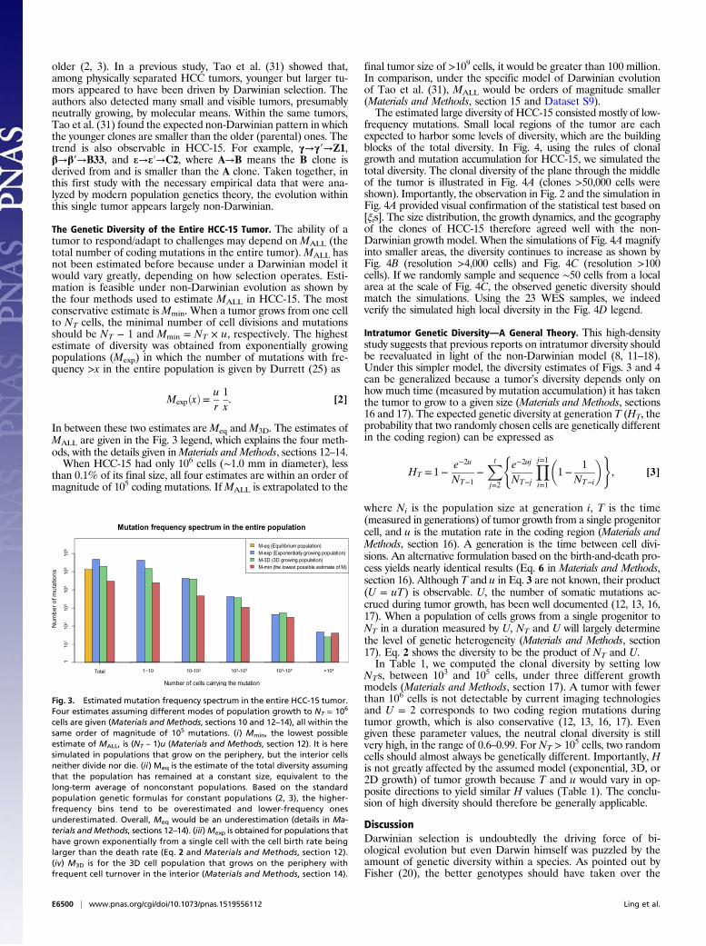
The Genetic Diversity of the Entire HCC-15 Tumor. The ability of atumor to respond/adapt to challenges may depend on MALL (thetotal number of coding mutations in the entire tumor).MALL hasnot been estimated before because under a Darwinian model itwould vary greatly, depending on how selection operates. Esti-mation is feasible under non-Darwinian evolution as shown bythe four methods used to estimate MALL in HCC-15. The mostconservative estimate isMmin. When a tumor grows from one cellto NT cells, the minimal number of cell divisions and mutationsshould be NT − 1 and Mmin = NT × u, respectively. The highestestimate of diversity was obtained from exponentially growingpopulations (Mexp) in which the number of mutations with fre-quency >x in the entire population is given by Durrett (25) as

MexpðxÞ= ur1x. [2]

In between these two estimates areMeq andM3D. The estimates ofMALL are given in the Fig. 3 legend, which explains the four meth-ods, with the details given inMaterials and Methods, sections 12–14.When HCC-15 had only 106 cells (∼1.0 mm in diameter), less

than 0.1% of its final size, all four estimates are within an order ofmagnitude of 105 coding mutations. IfMALL is extrapolated to the

final tumor size of >109 cells, it would be greater than 100 million.In comparison, under the specific model of Darwinian evolutionof Tao et al. (31), MALL would be orders of magnitude smaller(Materials and Methods, section 15 and Dataset S9).The estimated large diversity of HCC-15 consisted mostly of low-

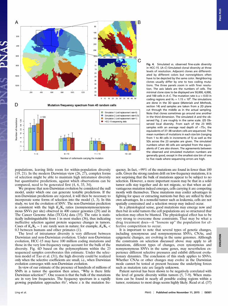
frequency mutations. Small local regions of the tumor are eachexpected to harbor some levels of diversity, which are the buildingblocks of the total diversity. In Fig. 4, using the rules of clonalgrowth and mutation accumulation for HCC-15, we simulated thetotal diversity. The clonal diversity of the plane through the middleof the tumor is illustrated in Fig. 4A (clones >50,000 cells wereshown). Importantly, the observation in Fig. 2 and the simulation inFig. 4A provided visual confirmation of the statistical test based on[ξis]. The size distribution, the growth dynamics, and the geographyof the clones of HCC-15 therefore agreed well with the non-Darwinian growth model. When the simulations of Fig. 4Amagnifyinto smaller areas, the diversity continues to increase as shown byFig. 4B (resolution >4,000 cells) and Fig. 4C (resolution >100cells). If we randomly sample and sequence ∼50 cells from a localarea at the scale of Fig. 4C, the observed genetic diversity shouldmatch the simulations. Using the 23 WES samples, we indeedverify the simulated high local diversity in the Fig. 4D legend.

Intratumor Genetic Diversity—A General Theory. This high-densitystudy suggests that previous reports on intratumor diversity shouldbe reevaluated in light of the non-Darwinian model (8, 11–18).Under this simpler model, the diversity estimates of Figs. 3 and 4can be generalized because a tumor’s diversity depends only onhow much time (measured by mutation accumulation) it has takenthe tumor to grow to a given size (Materials and Methods, sections16 and 17). The expected genetic diversity at generation T (HT, theprobability that two randomly chosen cells are genetically differentin the coding region) can be expressed as

HT = 1−e−2u

NT−1−

Xt

j=2

(e−2uj

NT−j

Yj=1i=1

�1−

1NT−i

�), [3]

where Ni is the population size at generation i, T is the time(measured in generations) of tumor growth from a single progenitorcell, and u is the mutation rate in the coding region (Materials andMethods, section 16). A generation is the time between cell divi-sions. An alternative formulation based on the birth-and-death pro-cess yields nearly identical results (Eq. 6 in Materials and Methods,section 16). Although T and u in Eq. 3 are not known, their product(U = uT) is observable. U, the number of somatic mutations ac-crued during tumor growth, has been well documented (12, 13, 16,17). When a population of cells grows from a single progenitor toNT in a duration measured by U, NT and U will largely determinethe level of genetic heterogeneity (Materials and Methods, section17). Eq. 2 shows the diversity to be the product of NT and U.In Table 1, we computed the clonal diversity by setting low

NTs, between 103 and 105 cells, under three different growthmodels (Materials and Methods, section 17). A tumor with fewerthan 106 cells is not detectable by current imaging technologiesand U = 2 corresponds to two coding region mutations duringtumor growth, which is also conservative (12, 13, 16, 17). Evengiven these parameter values, the neutral clonal diversity is stillvery high, in the range of 0.6–0.99. For NT > 105 cells, two randomcells should almost always be genetically different. Importantly, His not greatly affected by the assumed model (exponential, 3D, or2D growth) of tumor growth because T and u would vary in op-posite directions to yield similar H values (Table 1). The conclu-sion of high diversity should therefore be generally applicable.

DiscussionDarwinian selection is undoubtedly the driving force of bi-ological evolution but even Darwin himself was puzzled by theamount of genetic diversity within a species. As pointed out byFisher (20), the better genotypes should have taken over the

Fig. 3. Estimated mutation frequency spectrum in the entire HCC-15 tumor.Four estimates assuming different modes of population growth to NT = 106

cells are given (Materials and Methods, sections 10 and 12–14), all within thesame order of magnitude of 105 mutations. (i) Mmin, the lowest possibleestimate of MALL, is (NT – 1)u (Materials and Methods, section 12). It is heresimulated in populations that grow on the periphery, but the interior cellsneither divide nor die. (ii) Meq is the estimate of the total diversity assumingthat the population has remained at a constant size, equivalent to thelong-term average of nonconstant populations. Based on the standardpopulation genetic formulas for constant populations (2, 3), the higher-frequency bins tend to be overestimated and lower-frequency onesunderestimated. Overall, Meq would be an underestimation (details in Ma-terials andMethods, sections 12–14). (iii)Mexp is obtained for populations thathave grown exponentially from a single cell with the cell birth rate beinglarger than the death rate (Eq. 2 and Materials and Methods, section 12).(iv) M3D is for the 3D cell population that grows on the periphery withfrequent cell turnover in the interior (Materials and Methods, section 14).

E6500 | www.pnas.org/cgi/doi/10.1073/pnas.1519556112 Ling et al.

populations, leaving little room for within-population diversity(19, 21). In the modern Darwinian view (26, 27), complex formsof selection might be able to maintain high intratumor diversitybut quantitative predictions, against which observations can becompared, need to be generated first (4, 6, 33, 34).We propose that non-Darwinian evolution be considered the null

model, under which one can generate testable predictions. If thenon-Darwinian predictions are rejected, it will then be necessary toincorporate some forms of selection into the model (1, 3). In thisstudy, we test the evolution of SNV. The non-Darwinian predictionis consistent with the high Ka/Ks ratios (nonsynonymous/synony-mous SNVs per site) observed in 400 cancer genomes (29) and inThe Cancer Genome Atlas (TCGA) data (35). The ratio is statis-tically indistinguishable from 1 in most studies (36), thus indicatingineffective selection against protein sequence changes in tumors.Cases of Ka/Ks ∼ 1 are rarely seen in nature; for example, Ka/Ks <0.3 between humans and other primates (1).The level of intratumor diversity is very different between

Darwinian and non-Darwinian evolution. Under non-Darwinianevolution, HCC-15 may have 100 million coding mutations andthose in the very low-frequency range account for the bulk of thediversity. Fig. 4D based on the polymorphisms within the 23sequenced samples corroborates this estimate. Under the selec-tion model of Tao et al. (31), the high diversity could be realizedonly when the selective coefficients are small, i.e., when Darwinianevolution converges with non-Darwinian evolution.In view of our estimate of the presence of hundreds of millions of

SNPs in a tumor the question then arises, “Why is there littleDarwinian selection?”. One reason is that the bulk of the mutationsare in very low frequencies. The frequency spectrum in a rapidlygrowing population approaches θ/x2, where x is the mutation fre-

quency. In fact, ∼99% of the mutations are found in fewer than 100cells. Given the strong random drift on low-frequency mutations, it isnot surprising that the bulk of mutations appear to be subject to noselection. However, a more important reason may be that in a solidtumor cells stay together and do not migrate, so that when an ad-vantageous mutation indeed emerges, cells carrying it are competingmostly with themselves. These mutations may confer advantages infighting for space or extracting nutrients but they are stifled by theirown advantages. In a nonsolid tumor such as leukemia, cells are notspatially constrained and a selection sweep may indeed occur.In a physiological sense, good mutations may emerge now and

then but in solid tumors the cell populations are so structured thatselection may often be blunted. The physiological effect has to bevery strong to overcome those constraints. That may be what adrug treatment does—it “loosens up” the population for ef-fective competition to occur.It is important to note that several types of genetic changes,

including synonymous and nonsynonymous SNVs, CNAs, andepigenetic changes, are evolving in the same genomes. Althoughthe constraints on selection discussed above may apply to allmutations, different types of changes, even synonymous andnonsynonymous SNVs in the same genes, may nevertheless ex-perience different selective pressures and exhibit different evolu-tionary dynamics. The conclusion of this study applies to SNVs.Whether CNAs or other changes may evolve in the Darwinianmode cannot be tested at present because the underlying forcessuch as mutation rate are largely unknown.Patient survival has been shown to be negatively correlated with

the level of genetic diversity within tumors (5, 7–9). When muta-tions can be found in nearly all possible coding regions within atumor, resistance to most drugs seems highly likely. Read et al. (37)

Fig. 4. Simulated vs. observed fine-scale diversityin HCC-15. (A–C) Simulated clonal diversity at threelevels of resolution. Adjacent clones are differenti-ated by different colors but nonneighbors oftenhave to be depicted by the same color. Neighboringclones usually differ by one to two coding muta-tions. The three panels zoom in with finer resolu-tion. The axis labels are the numbers of cells. Theminimal clone sizes to be displayed are 50,000, 4,000,and 100 cells in A–C. The mutation rate is u = 0.03 incoding regions and NT = 1.15 × 109. The simulationsare done in the 3D space (Materials and Methods,section 14) and samples are taken from a 2D planecut through the middle as in the actual sampling.Note that clones sometimes go around one anotherin the third dimension. The simulated A and the ob-served Fig. 2 are roughly in the same scale. (D) Ob-served local diversity. From each of the 23 WESsamples with an average read depth of ∼75×, theequivalents of 37–38 random cells are sequenced. Themean numbers of mutations in each size bin (rangingfrom 1 to 40 cells in increments of 5) as well as theSDs across the 23 samples are given. The simulatednumbers when 40 cells are sampled from the equiv-alents of C are also shown. The agreements betweenthe observed and simulated mutation numbers aregenerally good, except in the smallest-size bin of oneto five reads where sequencing errors are high.

Ling et al. PNAS | Published online November 11, 2015 | E6501

EVOLU

TION

PNASPL

US

pointed out that aggressive strategies against cancerous cells areeffective only in the absence of resistance at treatment and variousstrategies for administering drugs in the face of resistant clones havebeen proposed (38–42). Finally, a key feature of the non-Darwinianmodel is the rapidity with which mutations accrue. Even micro-scopic tumors with fewer than 105 cells, which are often targets ofpostsurgery adjuvant therapy, would be genetically diverse (Table1). The possibility of high intratumor diversity even in small tumorssuggests a need to reevaluate treatment strategies.

Materials and MethodsThe following sections present essential technical information that is referredto asMaterials and Methods, sections 1–17 in the text. Additional details canbe found in Supporting Information).

1) Clinical Information. The patient was a 75-y-old man with chronic HepatitisB Virus (HBV) infection and liver cirrhosis. The tumor, ∼35 mm in diameter,was on the left lobe of the liver and well encapsulated. It was a histopath-ological grade III hepatocellular carcinoma (HCC) diagnosed at Peking Uni-versity Cancer Hospital. The pathology report indicated that the tumorsections contain ∼90% hepatoma cells. Two sections of 35 × 35 × 10 mmfrom the tumor and an adjacent nontumor sample were obtained. This studywas approved by the Ethics Review Committee of Peking UniversityCancer Hospital. Informed consent was signed according to the regulationsof the institutional ethics review boards.

2) Number, Volume, and Geographical Distribution of Samples. The honey-comb-like sampling is further described in Fig. S1. One 1-mm-thick slice of thetumor sample was subjected to high-density microdissection, using theHarris Micropunch with 0.5 mm inner diameter. In total, 286 microsectionswere obtained, equally distributed in the four quadrants (labeled A–D; Fig.S1). An adjacent nontumor sample was used as the control. Genomic DNAwas extracted using the TIANampMicro DNA Kit (Tiangen) and quantifiedusing a Qubit 2.0 fluorometer according to the manufacturer’s instructions.

Special attention was paid to minimizing the sample volume (number of cellsper sample) as genealogical information is better preserved in samples of smallervolume. Given that the diameter of aHCC cell is about 25 μm(20–30 μm), and thevolume of a microsection is ∼0.2 mm3, the number of cells in a microsection wasestimated to be ∼24,000. DNAwas extracted and quantified from 10,000 tumorcells that were precisely collected by laser capture microdissection (LCM). Thecell number in each of the microsections was estimated based on the referencequantity. For the 286 microsections, the median number of cells per sample was∼20,000, which approximates the number estimated by volume (Fig. S2).

3) Detection of Copy Number Alterations and Estimation of Tumor Purity.CAScnv (an in-house software) was used to detect the somatic copy num-ber alterations (Supporting Information). We used ABSOLUTE (49) (www.broadinstitute.org/cancer/cga/ABSOLUTE) to infer the purity and ploidy forour samples. The copy number alterations called from whole-exome se-quencing reads using CAScnv were input into the ABSOLUTE program (49). Basedon precomputed models of recurrent cancer karyotypes, the ABSOLUTE al-gorithm examined possible mappings from relative to integer copy numbersby jointly optimizing two parameters, α  (purity) and τ (ploidy). The inferredtumor purity and ploidy of all 23 tumor samples are shown in Dataset S1,which are consistent with the estimates in the pathology report.

4) Detection of Somatic SNV. Tagmentation-based library preparation (Fig. S7),WES, and sequence alignment are described in Supporting Information. SomaticSNV calling was performed using the in-house software, CASpoint, which hasbeen extensively tested in the public domain (Dataset S10; also see the result inthe International Cancer Genome Consortium-TCGA DREAM Somatic MutationChallenge (SMC): https://www.synapse.org/#!Synapse:syn312572/wiki/70726).We compared the false positive and negative rates, sensitivity, and accuracy ofCASpoint in SNV calling with the performances of other published softwareinstalled in the Beijing Institute of Genomics (BIG) computational center andbioinformatics facility, including Mutect (43), SomaticSniper (44), JoinSNVmix(45), Varscan2 (46), and Samtools (47). Simulated sequencing reads in the SMCand a large set of whole-genome or -exome sequencing reads produced fromvarious genomics projects in solid tumors (31) and leukemia (48) in Beijing In-stitute of Genomics were used to evaluate the performance of CASpoint. Theoverall accuracy of CASpoint is comparable to the others for the SMC simulatedreads. Because CASpoint showed better performance in reducing false positiverates than other programs for real sequencing data according to validation

results using Sequenom and Sanger sequencing, the in-house program wasused in this study to minimize the false positive rate.

As described in Zhu et al. (48), two statistical tests are introduced in theprogram. One-sided Fisher testing calculates the statistical significance oftumor mutant allele frequency (MAF) that is higher in the tumor populationthan in the normal cell population. Binomial testing calculates the signifi-cance of tumor mutant allele number observed from the aligned tumorsequencing data that meet a binomial distribution. In addition, 10 filteringcriteria were applied to detect somatic SNVs as described in Supporting In-formation. All somatic mutations are shown in Dataset S2.

5) Validation of the Observed SNVs Across the 286 Samples. SNVs discovered byWES were validated by Sequenom genotyping on the 286 samples. These dis-covered SNVs fall into three classes: (i) The ALL class has 178 SNVs that were dis-covered in all 23 WES samples (all red dots in Fig. 1A), (ii) the MOST class has 53SNVs that were present in most samples and missing in only a few (usually 1–4where read depthwas low), and (iii) the SOME class has 38 SNVs thatwere presentin some (≤6 samples; Fig. 1B) but missing in all other samples. These partitions areshown in Fig. S4 and the mutant allele frequencies are shown in Dataset S2.

The three classes ofmutations (ALL, MOST, and SOME) require different levelsof efforts of validation by Sequenomgenotyping: (i) For the 178mutations in theALL class, their ubiquity is certain. We chose 3 of these mutations for validationin the 286 samples and confirmed their ubiquity. (ii) The 53 mutations in theMOST class were validated in the few WES samples where they were foundmissing. In samples where the mutant was missing due to low read depth,Sequenom confirmed the presence of these 31 mutations (Dataset S2). There are22 ambiguous cases where the mutant is missing in 1–3 samples that have copynumber alterations in the regions of the mutations. These are likely cases of lossof heterozygosity (LOH). Although we suspect the mutations to be “possiblyfixed” with a few LOH samples, these 22 mutations are not included in sub-sequent analyses. (iii) The 38mutations in the SOME class were validated in all ormost of the 286 samples. The results are shown in Dataset S3. Of the 38 mu-tations, 3 could not be reliably detected across samples due to PCR difficulties.Hence, we analyzed only the remaining 35 mutations as true polymorphisms.

We used the SequenomMassARRAY Assay Design 3.1 software to design thePCR andMassEXTEND primers (Dataset S11) for multiplexed assays. MassEXTENDreactions and iPLEX Gold assays were subsequently used for primer extensionand allele frequency measurement. The allele-specific extension products fordifferent allelic types were quantitatively analyzed, using the MALDI-TOF massspectrometer. Using the mutant signal of nontumor as a negative control, mu-tation calling and allele frequencies for each SNV site were determined using theMassArrayTyper 4.0 Analyzer according to the manufacturer’s specifications. Toestimate mutant allele frequency and degree of heterozygosity, the peak areasof the mutant and the wild-type allele were quantified and the mutant allelefrequencies were determined as the average of (mutant peak)/(mutant peak +wild-type peak). We wrote scripts to extract mutation frequencies from Seque-nom Typer 4.0 software. Genomic positions for all validation SNVs were re-trieved using the HG19 as reference. Some SNVs found in only one sample werefurther validated by PCR and Sanger sequencing (Supporting Information).

6) Identification of Fixed and Polymorphic Somatic Mutations. Based on thedescriptions inMaterials and Methods, section 4 and the results of Datasets S2and S3 and Fig. S4, the 269 SNVs are classified as 209 confirmed fixed SNVs, 35confirmed polymorphic SNVs, and 25 less certain mutations. These 25 muta-tions, including respectively 22 possible fixed and 3 possible polymorphicmutations, were not used in the analyses. The partition of these 269 SNVssummarized in Fig. S4 is as follows:

i) The confirmed 209 fixed mutations include 178 from the ALL class and 31from the MOST class described inMaterials and Methods, section 4 above.The 178 SNVs were observed in all 23 WES samples (Dataset S2) and thelimited validation among unsequenced samples indeed confirmed theirubiquitous presence. The 31 MOST class mutations were present in all buta few (1–4) WES samples, due to low depth coverage of such sites in thesesamples. Sequenom results validated their presence in these samples.

ii) The 35 confirmed polymorphic mutations are listed in Dataset S2 amongWES samples. They were further validated across the 286 samples bySequenom (and occasionally by Sanger sequencing) as shown in DatasetS3, which is the basis of the spatial distribution of these mutationsshown in Figs. 1 and 2 of the main text.

iii) For the remaining 25 SNVs, 22 mutations are missing in 1–4 samples(Dataset S2, under “SNV in CNA regions”). These mutations occurredin regions of frequent CNAs, which would result in LOH. LOH could beinferred directly from these data when AB (mutations A and B occurredin 20 samples), A+ (mutation A but not B occurred in 2 samples), and +B

E6502 | www.pnas.org/cgi/doi/10.1073/pnas.1519556112 Ling et al.

(mutation B but not A occurred in 1 sample) were all observed. In thispattern, B is lost twice and/or A is lost once. From the pattern shown inDataset S2, it is likely that all of the 22 mutations are fixed but it isprudent to exclude them from subsequent analyses, as was done here.

iv) The 3 possibly polymorphic mutations were detected in someWES samplesbut could not be reliably genotyped across the 286 samples by Sequenom.They are almost certainly polymorphic mutations but could not be used inthis study to delineate the spatial boundaries of clones or their sizes.

7) Clone Map Delineation and Phylogenetic Analysis. The 35 polymorphic SNVsunaffected by CNAs were validated in the 286 tumor samples, using Sequenomand/or Sanger sequencing (Dataset S3). The neighbor-joining method of Saitouand Nei (50) was used to construct the phylogenetic tree (Fig.1 B and D). Aconsolidated matrix was created, containing the mutations of all samples with“1” and “0” representing the presence and absence of a mutation based ongenotyping results of the 35 SNVs. We used the “APE” R package (51) and iTOL(itol.embl.de) for constructing and plotting the phylogenetic trees (Fig. 1 B andD). The positions of eight samples (A3, B17, B19, B20, C78, D6, D9, and Z1) thatcarried mutations of two neighboring clones were marked with blue stars inthe phylogenic tree in Fig. 1D. The boundaries and space of the subclones inHCC-15 were delineated in the two-dimensional clonal map based on both thepresence of the polymorphic SNVs and the phylogenic relationship (Fig. 2).

8) Identification of Putative “Driver” Genes. We attempted to identify drivergenes from among the 269 mutated genes in our study. As in commonpractice, driver genes are defined as those that are significantly over-represented in the cancer databases. The data we used here comprise 460,967somatic mutations (402,716 SNVs, 42,886 small deletions, and 12,249 smallinsertions) detected in whole-exome sequencing data of 1,363 patients withgastrointestinal cancer (Dataset S6), including 202 hepatocellular carcinoma(LIHC) (72,862 mutations), 183 esophageal carcinoma (ESCA) (54,042 muta-tions), 288 stomach adenocarcinoma (STAD) (115,357 mutations), 220 colonadenocarcinoma (COAD) (114,594 mutations), 81 rectum cancers (READ)(25,003 mutations), and 147 pancreas cancers (PAAD) (56,815 mutations) fromTCGA datasets and 242 hepatocellular carcinomas (22,294 mutations) in Schulzeet al. (32). We applied the program MutSigCV 1.4 (52), which corrects for var-iation by incorporating a patient-specific mutational spectrum and gene-specific background mutational burden, and by measuring gene expressionand replication time as well, to detect significantly mutated genes.

In total, we identified 372 driver genes from the somatic mutations dataset of1,363 gastrointestinal cancer cases (Dataset S5). Comparing the 166 fixed pro-tein-altering mutations in our study to the driver genes identified from thedatabases, we identify 6 putative driver genes (q-value ≤ 0.2): CCAR1, CPXM2,DNAH7, TMPRSS13, TSC1, and TP53; the last of the 6 genes has a high fre-quency in all gastrointestinal cancers (Fig. S5). We note that none of the genescarrying any of the 35 polymorphic mutations in this study belongs in the drivergroup. Ingenuity pathway analysis (IPA) (www.ingenuity.com) and Fisher’s ex-act test were carried out to identify significantly enriched pathways for thegenes with polymorphic and fixed protein-sequence altering SNVs (Dataset S5).

9) Observed Mutation Frequency Spectrum. The mutation frequency spectrumis denoted as [ξi, i = 1 to n − 1] in the main text, ξi is the number of siteswhere the mutant appears i times in n samples in the infinite-site model ofpopulation genetics. In Fig. 1B, the heat map is equivalent to a spectrum of[ξi = 24, 2, 3, 2, 1, 3, 0, 0, . . .] for i = 1–22, where Σiξi = 35 is the numberof mutations in the 23 WES samples. In this spectrum, the mutation in eachsample is scored as either present or absent.

Because the frequency of each mutation was more accurately determined bygenotyping, ξi is represented by the number of sites where the frequency of themutation was between (i − 1)/23 and i/23 from the 286 samples. We kept thenumber of frequency bins at 23 because themutations discovered were still basedon the initial 23 samples. The spectrum, as given in Dataset S8, is [ξi = 26, 7, 1, 1, 0,0, . . .] for i = 1–22. There are two methods to compute the frequency spectrumusing the data from the 286 samples. One is to score the presence/absence of eachmutation in each sample. This will tend to inflate the frequencies of themutationsas samples with only a fraction of cells carrying themutation would be scored as afull site. To obtain the spectrum of [ξi = 26, 7, 1, 1, 0, 0, . . .], we used a secondmethod by averaging the frequency of each mutation over all samples.

Finally, Fig. 4D presents local diversity by scoring mutations that have lowercounts in each WES sample. In calling such mutations, stringent validation isnecessary to determine the level of confidence, which would be lower as thefrequency decreases. At 21 of 22 sites, SNV calls based on 6–10 mutant readswere validated by Sequenom genotyping (Dataset S2), a validation rate of95.5%. SNV calls supported by >10 reads are accurate with a 99% validation

rate. The validation rates suggest that the calls in bins >5 reads are of highconfidence. We disregard calls with ≤5 reads in Fig. 4D, which gives the meanand SD of mutation number in each of the larger size bins.

10) Expected Mutation (Site) Frequency Spectrum in Exponentially GrowingPopulations.

Eξn,i ≈

8>>>><>>>>:

nur

XNT r

k=1

1n+ k

kn+ k− 1

i= 1

nur

1iði−1Þ 2≤ i<n,

[4]

where r is the rate of exponential growth, u is the mutation rate per cellgeneration, n is the sample size, and NT is the cell population size at time T(25). For HCC-15, [ξ23,i = 26, 7, 1, 1, 0, 0, . . .; i = 1–22]. Because Σi>1ξ23,i = (7 +1 + 1) = 9 = 23 u/r, we obtain u/r = 0.41. The expected site frequency spectrumfor 35 mutations is hence [E(ξ23,i) = 26.0, 4.72, 1.57, 0.79, 0.47, 0.31,. . .].

11) Max (k)s—Frequency of the Most Common k Mutations in a Sample. We notethat the observed frequency spectrum given in the main text is [ξi = 26, 7, 1, 1, 0,0, . . .] for i = 1–22. Hence, the average frequency of the k most common muta-tions would be 4, (4 + 3)/2, and (4 + 3 + 2)/3 for k = 1–3, respectively. BecauseDarwinian selection would drive the advantageous mutations to a high fre-quency (19, 21), it would be informative to compare the observed frequencies ofthemost common kmutations with those expected for the detection of selection.

Under the neutral model, we can determine the average frequency of themostcommon k mutations in our sample, denoted Max(k). E(ξn,i) is the expected num-ber of mutations that were found in i of the 23 samples. In exponentially growingpopulations, the corresponding E(ξn,i) has been defined by Durrett (25) as Eq. 1,

E�ξn,i

�≅nur

1iði− 1Þ  2≤ i<n,

where r is the rate of population growth, the difference between cell birthand death (main text). For the total of 35 sites, [E(ξn,i) = 26.0, 4.72, 1.57, 0.79,0.47, 0.31, . . .] which sum up to 35. We took 35 mutations from this distri-bution and determined the Max(k) for k = 1–4. The distributions of Max(k) in10,000 repeats are given in Fig. S6. For example, the 95% cutoff for k = 1 (i.e.,the most common mutation) would be 20 of 23 samples. Likewise, the 95%cutoff for k = 3 (the average frequency of the top 3 common mutations)would be 12 as presented in the main text.

12) Four Estimates of the Total Number of Mutations (MALL). The minimal numberof mutations accrued during tumor growth was referred to asMmin. When cellsof a tumor divide from 1 to NT cells, the minimal number of cell divisions shouldbe NT − 1, if no cells die during tumor growth, resulting in Mmin = NT × u. Wecarried out computer simulations in which tumors grew outward as a 3D mass.In our model, cells were “frozen” when they become encapsulated inside thetumor; only cells on the periphery were able to divide (Materials and Methods,section 14). This mode of growth does not require manymore cell divisions thanthe minimum of NT − 1. Fig. 3 shows that the number of mutations under sucha growth mode, with NT = 106 and u = 0.03 (per cell division in the codingregion, equivalent to 10−9 per cell division per base pair), was very close to theminimum of Mmin = NT × u = 3 × 104 mutations. Even at this minimum, MALL

was substantial. The choice of u = 0.03 is in agreement with several previousstudies (18, 24), as well as with the estimate by the approximate Bayesiancomputation (ABC) method (Supporting Information and Fig. S8).

The secondmethodused to estimateMALLwas to assume that the cell populationwas maintained at a constant size, close to the long-term average of changingpopulation sizes. Standard population genetic formulaes can then be used to esti-mate the equilibrium genetic diversity,Meq, analytically (2, 3). Nevertheless, becausethe cell population is likely to have been growing, Meq would almost always un-derestimate the true diversity. This is because the imposition of the equilibriumconditions on the data would result in adequate estimation of diversity only in theobservable portion of the spectrum. Low-frequency mutations were expected to beunderestimated. In Materials and Methods, section 13, we provide the details ofobtaining Meq, as well as the simulation data that corroborated the conjecture ofMeq<MALL. Asmost tumors are growing, albeit not necessarily in any specificmode,Meq should be a reasonable lower bound of a tumor’s diversity. For HCC-15, Meq

was roughly 14% of NT and substantially larger than Mmin as shown in Fig. 3.In the third estimate, Mexp, the mode of population growth is specified. If

cells divide and die at a constant rate, the population would be growingexponentially. The net growth (i.e., the difference between the birth anddeath rates) could be positive, negative, or net zero. Under this exponential

Ling et al. PNAS | Published online November 11, 2015 | E6503

EVOLU

TION

PNASPL

US

model developed by Durrett (25), the number of mutations with frequency>x in the entire population is given by Eq. 2.

The elegant simplicity of Eq. 2 is not unexpected because the geneticdiversity in a tumor is largely determined by two parameters: the number ofmutations (U) each cell accumulates during tumor growth and the pop-ulation size (NT = erT). The expression, U = uT = (u/r) ln(NT), thus anticipatesthe simplicity. The total number of mutations in the tumor, Mexp(x = 1/NT), isprojected to be (u/r) × 1/(1/NT). From the observed mutation frequencyspectrum [ξis] and Eq. 1, we have obtained u/r = 0.41.

Given NT = 106 cells, HCC-15 would have Mexp= 4.1 × 105 coding muta-tions (Fig. 3), which was more than 10-fold larger than Mmin. The mutationfrequency spectrum is also given in Fig. 3. Even for such a small tumor, therewould still be 5,000 mutations, each of which can be found in more than 100cells. In a different approach to estimating u/r, we used an approximateBayesian computation method (53) by simulating a branching process withcell birth, death, and mutation often used for modeling tumor growth (54).We obtained the posterior mean u and r that showed u/r = 0.412 (Fig. S8),which was nearly equal to 0.41 obtained from Eq. 1.

In the fourth estimate, M3D, the growth mode is also specified and the in-crease in cell number is assumed to occur only on the periphery of a tumor in3D (Materials and Methods, section 14). In the interior, each cell division resultsin the birth of one cell, which would replace a neighboring cell. Because thebirths and deaths cancel out in the interior, the growth rate of the tumor(dN/dt) is proportional to N2/3, instead of N as in the exponential growth. Simu-lation results of Fig. 3 showed that the 3D growthmode yielded similar mutationnumbers Mexp, except in the lowest-frequency bin of fewer than 10 cells.

13) Computer Simulations of Meq, a lower bound of MALL. Meq is the number ofmutations in the population by artificially imposing the mutation–drift equi-librium on the tumor. Thus, Meq = θ ln(NT), where θ = 2Neu is the scaledmutation parameter in tumor growth and Ne is the effective cell populationsize. We implemented computer simulations to prove that Meq is a properlower bound of mutation numberM in a growing population.Meq is expectedto always be smaller than M under any mode of tumor growth. Three typicalgrowth models were simulated, including exponential growth, 2D growth,and 3D growth. It should be noted that the cell populations with models of 2Dgrowth (dN/dt = r N1/2) and 3D growth (dN/dt = r N2/3) are essentially wellmixed and belong to the power law family of tumor growth models.

For exponential growth, we simulated a discrete-time birth–death process,in which an individual divides and gives birth to two daughter cells withprobability b and dies with probability d (b + d = 1) in each generation.Hence the expected exponential growth rate r = ln(2b). In simulation of 2Dgrowth or 3D growth, the birth probability varied with time, depending onthe population size N(t). In particular, birth probability b = (1 + r/N(t)1/2)/2and (1 + r/N(t)1/3)/2, respectively, for 2D growth and 3D growth, where r isthe factor determining the growth rate.

Because Meq = θ ln(NT) and θ is unknown, we use the maximum-likelihoodmethod based on the Ewens sampling formula to estimate θ under a particulargrowth model and associated parameters (2). To do this, we need to know theallele frequency spectrum, which can be obtained by randomly sampling23 cells at a time from NT = 105 cells (i.e., similar to sampling 23 cell populationsfor exome sequencing in HCC-15). Therefore, we can obtain both M and Meq.Mutation rate u = 0.03 (the whole coding region) was applied in all of thesimulations. In each model, 20 simulations were implemented and the averagewas treated as the estimate for the mutation numbers M and Meq (Fig. S9).

14) Simulation of Genetic Diversity in Growing Populations. To simulate theclonal diversity in a tumor and to compare with the theoretical predictions, wedesigned cellular automata models (55, 56) to simulate tumor expansion andmutation accumulation in 3D space.

15) The Expected Frequency Spectra Under Selection. Here, we develop amodel of selection to compare the total genetic diversity under Darwinianand non-Darwinian evolution (SI Theory). The full model was developed tostudy the evolution of tumor size (31) with selection and migration. Becausethe dynamics with migration are the same as those with mutation, themodel is interchangeable for mutation and migration (31).

16) Mathematical Derivation of Clonal Diversity HT. LetNt be the population sizeat generation t and u be mutation rate per generation in the coding region ofthe human genome. We denote by Pr(coalescence) the probability that tworandomly chosen cells at generation t find their common ancestor at generationt − 1. And we denote by Jt the probability that two random cells are geneticallyidentical at generation t (1 − Jt is equivalent to Simpson’s diversity index).

Jt can be expressed as a recursive formula:

Jt = ð1−uÞ2 × ½PrðcoalescenceÞ+ ð1− PrðcoalescenceÞÞJt−1�.

In a Wright–Fisher growing population, Pr(coalescence) can be approximatedby 1/Nt−1, and thus

Jt = ð1−uÞ2 ×�

1Nt−1

+�1−

1Nt−1

�Jt−1

�, [5]

which can be solved by substituting Ji by Ji−1 successively:

Jt =1

Nt−1ð1−uÞ2 +

Xt

j=2

1Nt−j

ð1−uÞ2j ∏j−1

i=1

�1−

1Nt−j

�+ J0ð1−uÞ2t ∏

t

i=1

�1−

1Nt−i

�.

If N0 = 1, the last term can be removed. Then

Jt =1

Nt−1ð1−uÞ2 +

Xt

j=2

1Nt−j

ð1−uÞ2j ∏j−1

i=1

�1−

1Nt−i

�.

When u is small, it can be approximated by

Jt =e−2u

Nt−1+

Xt

j=2

e−2uj

Nt−j∏j−1

i=1

�1−

1Nt−i

�.

Therefore, the expected clonal diversity H, the probability that two ran-dom cells or cell clones are genetically different, at time T will be

HT = 1− JT = 1−e−2u

NT−1−

XTj=2

(e−2uj

NT−j∏j−1

i=1

�1−

1NT−i

�),

which is Eq. 3.The Wright–Fisher model of tumor growth assumes Poisson distribution for

the number of offspring cells that a cell generates in a division, whichmay not berigorous in modeling cell dynamics. To investigate the generality of Eq. 3, we alsoderived the exact formula of clonal diversity (HT) under a discrete-time birth–death process of tumor growth. In particular, a cell gives birth to two daughtercells with probability a and dies with probability b (a + b = 1) in a generation.The population grows exponentially with an expected population size of Nt =N0(2a)

t at time t. We are primarily interested in a lineage that starts with onesingle cell and propagates in a total of t generations. Therefore, N0 = 1 and Nt =(2a)t. Suppose two cells are randomly selected from generation t; the probabilitythat coalescence occurs in the previous generation between the two cells is Pr(coalescence) = 1/(Nt − 1). Solving previous recursion in the same way gives rise to

HT =1−e−2u

NT − 1−

XTj=2

(e−2uj

NT+1−j − 1∏j−2

i=0

�1−

1NT−i − 1

�). [6]

17) Estimating Clonal Diversity, HT, Under Different Growth Models. Eq. 3 canbe applied to arbitrary time variable-size cell populations. However, weexamined three models in this study to estimate the clonal diversity HT in agrowing cell population (Dataset S8), including an exponential growthmodel and two power-law growth models (resembling 2D and 3D growth,respectively).

In the exponential model, the population dynamics follow dN/dt = r*N incontinuous time. It can be solved as Nt = ert. In discrete time, r = ln(2) cor-responds to the situation that all cells duplicate with no cell death in eachgeneration. We showed the results using two growth rate values as r = ln(2) ×0.1 and r = ln(2) × 0.01, respectively. The other two models, 2D growth (dN/dt =rN1/2) and 3D growth (dN/dt = rN2/3), belong to the power-law family of tumorgrowth models. In these two models, r = 2π1/2 and r = (36π)1/3 correspondto the condition that the population generates exactly one layer of cells inthe periphery in each discrete generation for 2D growth and 3D growth,respectively. In the 3D growth model, two growth rate values were tested,where r = (36π)1/3 × 0.1 and r = (36π)1/3 × 0.01.

We set NT at three levels between 103 and 105 cells and Nis for i between0 and T, depending on which of the three growth models were used. Once thegrowth model and the r value were defined, the number of cell divisions re-quired to reach NT could be calculated. We calculated the expected clonaldiversity HT from Eq. 3 (Table 1).

ACKNOWLEDGMENTS. We are grateful to Nick Navin, Steve Frank, NellyPolyak, Carlo Maley, Robert Gatenby, Rick Durrett, Thomas Nagylaki, TianXu, Jianzhi (George) Zhang, Andy Clark, Xionglei He, and Yang Shen forinputs in various phases of this work. This study was supported by theNational Basic Research Program (973 Program) of China (2014CB542006to C.-I.W.), Research Programs of the Chinese Academy of Sciences

E6504 | www.pnas.org/cgi/doi/10.1073/pnas.1519556112 Ling et al.

(XDB13040300 and KJZD-EW-L06-1 to X.L. and C.-I.W.), the NationalScience Foundation of China (91131903 to X.L., 31301036 and 91231204to Z.Y.), the National High-Tech R&D Program (863 Program) of China

(2012AA022502 to X.L.), and the 985 Project (33000-18811202 to C.-I.W.)and Science Foundation of State Key Laboratory of Biocontrol(SKLBC15A37 to C.-I.W.).

1. Wen-Hsiung L (1997) Molecular evolution (Sinauer Associates Inc., Sunderland, MA).2. Ewens WJ (2010) Mathematical Population Genetics 1: Theoretical Introduction

(Springer, New York).3. Hartl DL, Clark AG (2006) Principle of Population Genetics (Sinauer, Sunderland, MA), 4th Ed.4. Nowell PC (1976) The clonal evolution of tumor cell populations. Science 194(4260):23–28.5. Maley CC, et al. (2006) Genetic clonal diversity predicts progression to esophageal

adenocarcinoma. Nat Genet 38(4):468–473.6. Merlo LMF, Pepper JW, Reid BJ, Maley CC (2006) Cancer as an evolutionary and

ecological process. Nat Rev Cancer 6(12):924–935.7. Marusyk A, Polyak K (2010) Tumor heterogeneity: Causes and consequences. Biochim

Biophys Acta 1805(1):105–117.8. Burrell RA, McGranahan N, Bartek J, Swanton C (2013) The causes and consequences

of genetic heterogeneity in cancer evolution. Nature 501(7467):338–345.9. Bedard PL, Hansen AR, Ratain MJ, Siu LL (2013) Tumour heterogeneity in the clinic.

Nature 501(7467):355–364.10. Bozic I, et al. (2010) Accumulation of driver and passenger mutations during tumor

progression. Proc Natl Acad Sci USA 107(43):18545–18550.11. Anderson K, et al. (2011) Genetic variegation of clonal architecture and propagating

cells in leukaemia. Nature 469(7330):356–361.12. Tao Y, et al. (2011) Rapid growth of a hepatocellular carcinoma and the driving

mutations revealed by cell-population genetic analysis of whole-genome data. ProcNatl Acad Sci USA 108(29):12042–12047.

13. Gerlinger M, et al. (2012) Intratumor heterogeneity and branched evolution revealedby multiregion sequencing. N Engl J Med 366(10):883–892.

14. Landau DA, et al. (2013) Evolution and impact of subclonal mutations in chroniclymphocytic leukemia. Cell 152(4):714–726.

15. Sottoriva A, et al. (2013) Intratumor heterogeneity in human glioblastoma reflectscancer evolutionary dynamics. Proc Natl Acad Sci USA 110(10):4009–4014.

16. de Bruin EC, et al. (2014) Spatial and temporal diversity in genomic instability pro-cesses defines lung cancer evolution. Science 346(6206):251–256.

17. Zhang J, et al. (2014) Intratumor heterogeneity in localized lung adenocarcinomasdelineated by multiregion sequencing. Science 346(6206):256–259.

18. Wang Y, et al. (2014) Clonal evolution in breast cancer revealed by single nucleusgenome sequencing. Nature 512(7513):155–160.

19. Fay JC, Wu CI (2000) Hitchhiking under positive Darwinian selection.Genetics 155(3):1405–1413.20. Fisher RA (1930) The Genetical Theory of Natural Selection (Clarendon, Oxford).21. Smith JM, Haigh J (1974) The hitch-hiking effect of a favourable gene.Genet Res 23(1):23–35.22. Vogelstein B, et al. (2013) Cancer genome landscapes. Science 339(6127):1546–1558.23. Garraway LA, Lander ES (2013) Lessons from the cancer genome. Cell 153(1):17–37.24. Jones S, et al. (2008) Comparative lesion sequencing provides insights into tumor

evolution. Proc Natl Acad Sci USA 105(11):4283–4288.25. Durrett R (2013) Population genetics of neutral mutations in exponentially growing

cancer cell populations. Ann Appl Probab 23(1):230–250.26. Kimura M (1984) The Neutral Theory of Molecular Evolution (Cambridge Univ Press,

Cambridge, UK).27. Nei M, Suzuki Y, Nozawa M (2010) The neutral theory of molecular evolution in the

genomic era. Annu Rev Genomics Hum Genet 11:265–289.28. Fay JC, Wyckoff GJ, Wu C-I (2002) Testing the neutral theory of molecular evolution

with genomic data from Drosophila. Nature 415(6875):1024–1026.29. Woo YH, Li W-H (2012) DNA replication timing and selection shape the landscape of

nucleotide variation in cancer genomes. Nat Commun 3:1004.30. Sottoriva A, et al. (2015) A Big Bang model of human colorectal tumor growth. Nat

Genet 47(3):209–216.31. Tao Y, et al. (2015) Further genetic diversification in multiple tumors and an evolu-

tionary perspective on therapeutics. BioRxiv:025429.32. Schulze K, et al. (2015) Exome sequencing of hepatocellular carcinomas identifies new

mutational signatures and potential therapeutic targets. Nat Genet 47(5):505–511.33. Cairns J (1975)Mutation selection and the natural history of cancer.Nature 255(5505):197–200.34. Greaves M, Maley CC (2012) Clonal evolution in cancer. Nature 481(7381):306–313.35. Kandoth C, et al. (2013) Mutational landscape and significance across 12 major cancer

types. Nature 502(7471):333–339.36. Ostrow SL, Barshir R, DeGregori J, Yeger-Lotem E, Hershberg R (2014) Cancer evolu-

tion is associated with pervasive positive selection on globally expressed genes. PLoSGenet 10(3):e1004239.

37. Read AF, Day T, Huijben S (2011) The evolution of drug resistance and the curious or-thodoxy of aggressive chemotherapy. Proc Natl Acad Sci USA 108(Suppl 2):10871–10877.

38. Catenacci DVT (2015) Next-generation clinical trials: Novel strategies to address thechallenge of tumor molecular heterogeneity. Mol Oncol 9(5):967–996.

39. Leder K, et al. (2014) Mathematical modeling of PDGF-driven glioblastoma revealsoptimized radiation dosing schedules. Cell 156(3):603–616.

40. LovenD, Hasnis E, Bertolini F, Shaked Y (2013) Low-dosemetronomic chemotherapy: From pastexperience to new paradigms in the treatment of cancer. Drug Discov Today 18(3-4):193–201.

41. Gatenby RA, Silva AS, Gillies RJ, Frieden BR (2009) Adaptive therapy. Cancer Res 69(11):4894–4903.

42. Silva AS, et al. (2012) Evolutionary approaches to prolong progression-free survival inbreast cancer. Cancer Res 72(24):6362–6370.

43. Cibulskis K, et al. (2013) Sensitive detection of somatic point mutations in impure andheterogeneous cancer samples. Nat Biotechnol 31(3):213–219.

44. Larson DE, et al. (2012) SomaticSniper: Identification of somatic point mutations inwhole genome sequencing data. Bioinformatics 28(3):311–317.

45. Roth A, et al. (2012) JointSNVMix: A probabilistic model for accurate detection of somaticmutations in normal/tumour paired next-generation sequencing data. Bioinformatics 28(7):907–913.

46. Koboldt DC, et al. (2012) VarScan 2: Somatic mutation and copy number alterationdiscovery in cancer by exome sequencing. Genome Res 22(3):568–576.

47. Li H, et al.; 1000 Genome Project Data Processing Subgroup (2009) The SequenceAlignment/Map format and SAMtools. Bioinformatics 25(16):2078–2079.

48. Zhu X, et al. (2014) Identification of functional cooperative mutations of SETD2 inhuman acute leukemia. Nat Genet 46(3):287–293.

49. Carter SL, et al. (2012) Absolute quantification of somatic DNA alterations in humancancer. Nat Biotechnol 30(5):413–421.

50. Saitou N, Nei M (1987) The neighbor-joining method: A new method for reconstructingphylogenetic trees. Mol Biol Evol 4(4):406–425.

51. Paradis E, Claude J, Strimmer K (2004) APE: Analyses of phylogenetics and evolution inR language. Bioinformatics 20(2):289–290.

52. Lawrence MS, et al. (2013) Mutational heterogeneity in cancer and the search for newcancer-associated genes. Nature 499(7457):214–218.

53. Beaumont MA, Zhang W, Balding DJ (2002) Approximate Bayesian computation inpopulation genetics. Genetics 162(4):2025–2035.

54. Durrett R (2015) Branching Process Models of Cancer (Springer, Cham, Germany), pp 1–63.55. Poleszczuk J, Enderling H (2014) A high-performance cellular automaton model of

tumor growth with dynamically growing domains. Appl Math 5(1):144–152.56. Waclaw B, et al. (2015) A spatial model predicts that dispersal and cell turnover limit

intratumour heterogeneity. Nature 525(7568):261–264.57. Adey A, et al. (2010) Rapid, low-input, low-bias construction of shotgun fragment

libraries by high-density in vitro transposition. Genome Biol 11(12):R119.58. Harbers M, Kahl G, Kahl G (2012) Tag-Based Next Generation Sequencing (Wiley, Weinheim,

Germany).59. Li H, Durbin R (2009) Fast and accurate short read alignment with Burrows-Wheeler

transform. Bioinformatics 25(14):1754–1760.60. Csilléry K, Blum MGB, Gaggiotti OE, François O (2010) Approximate Bayesian com-

putation (ABC) in practice. Trends Ecol Evol 25(7):410–418.61. Csilléry K, François O, Blum MGB (2012) abc: An R package for approximate Bayesian

computation (ABC). Methods Ecol Evol 3:475–479.62. Iwasa Y, Michor F (2011) Evolutionary dynamics of intratumor heterogeneity. PLoS One

6(3):e17866.63. Yachida S, et al. (2010) Distant metastasis occurs late during the genetic evolution of

pancreatic cancer. Nature 467(7319):1114–1117.64. Navin N, et al. (2011) Tumour evolution inferred by single-cell sequencing. Nature

472(7341):90–94.65. Xu X, et al. (2012) Single-cell exome sequencing reveals single-nucleotide mutation

characteristics of a kidney tumor. Cell 148(5):886–895.66. Nei M (2013) Mutation-Driven Evolution (Oxford Univ Press, Oxford).67. McDonald JH, Kreitman M (1991) Adaptive protein evolution at the Adh locus in

Drosophila. Nature 351(6328):652–654.68. Novembre J, et al. (2008) Genesmirror geographywithin Europe.Nature 456(7218):98–101.69. Hill WG, Robertson A (2007) The effect of linkage on limits to artificial selection. Genet

Res 89(5-6):311–336.70. Gerrish PJ, Colato A, Perelson AS, Sniegowski PD (2007) Complete genetic linkage can

subvert natural selection. Proc Natl Acad Sci USA 104(15):6266–6271.

Ling et al. PNAS | Published online November 11, 2015 | E6505

EVOLU

TION

PNASPL

US