extreme value theory i abdelmahamoud youssuf …

STATUS OF THESIS

Title of thesis

PREDICTING INTERNET TRAFFIC BURSTS USING

EXTREME VALUE THEORY

I ABDELMAHAMOUD YOUSSUF DAHAB hereby allow my thesis to be placed at the Information Resource Center (IRC) of

Universiti Teknologi PETRONAS (UTP) with the following conditions:

1. The thesis becomes the property of UTP 2. The IRC of UTP may make copies of the thesis for academic purposes only. 3. This thesis is classified as

Confidential

X Non-confidential

If this thesis is confidential, please state the reason: __________________________________________________________________________________________________________________________________________

The contents of the thesis will remain confidential for ___________ years. Remarks on disclosure: __________________________________________________________________________________________________________________________________________

Endorsed by ________________________________ __________________________ Signature of Author Signature of Supervisor Permanent address: Name of Supervisor

P.O Box 3151, Assoc. Prof. Dr. Abas MD

N’djamena, Republic of Chad Said

Tel. (+235)22511531

Date : _____________________ Date : __________________

UNIVERSITI TEKNOLOGI PETRONAS



by

ABDELMAHAMOUD YOUSSOUF DAHAB

The undersigned certify that they have read, and recommend to the Postgraduate Studies Programme for acceptance this thesis for the fulfilment of the requirements for the degree stated.

Signature: ______________________________________ Main Supervisor: ASSOC. PROF. DR. ABAS MD SAID Signature: ______________________________________ Co-Supervisor: DR. HALABI BIN HASBULLAH Signature: ______________________________________ Head of Department: DR. MOHD FADZIL BIN HASSAN

Date: ______________________________________



by

ABDELMAHAMOUD YOUSSOUF DAHAB

A Thesis

Submitted to the Postgraduate Studies Programme

as a requirement for the Degree of

DOCTOR OF PHILOSOPHY

COMPUTER AND INFORMATION SCIENCES DEPARTMENT

UNIVERSITI TEKNOLOGI PETRONAS

BANDAR SERI ISKANDAR,

PERAK

MAY 2011

iv

DECLARATION OF THESIS

Title of thesis

Predicting Internet Traffic Bursts using Extreme Value Theory

I ABDELMAHAMOUD YOUSSOUF DAHAB

hereby declare that the thesis is based on my original work except for quotations and

citations which have been duly acknowledged. I also declare that it has not been

previously or concurrently submitted for any other degree at UTP or other institutions.

Witnessed by ________________________________ __________________________ Signature of Author Signature of Supervisor Permanent address: Name of Supervisor

P.O Box 3151, N’djamena Assoc. Prof. Dr. Abas MD

Republic of CHAD Said

Date : _____________________ Date : __________________

v

ACKNOWLEDGEMENTS

Many thanks to those who helped me successfully finishing my doctoral program

and conducting my Graduate Assistant duties at Universiti Teknologi PETRONAS. In

particular, I thank my supervisor A.P. Dr Abas bin Md Said for his guidance,

patience, and support throughout the ups and downs of this thesis. Many thanks to Dr.

Halabi bin Hasbullah, my co-supervisor who introduced me to this field of research

and provided me with all the necessary support and insight into computer networks.

However, being a graduate student at UTP is a joy by itself. This is especially true

if you are working with wonderful people like Ms Penny Goh, Dr. Zulkiphli Ghazali,

and A.P. Dr. Abas. I thank them all for entrusting me with their classes and for many

other services they provided me with. I thank the head of CIS Department for his

support without forgetting all the P.G. Office personnel, who were always welcoming

and supportive. Special thanks go to PETRONAS Joint Venture for providing this

opportunity to Chadian scholars. It is such a great contribution to the Human Capital

Development of the Republic of Chad.

This whole work is dedicated to Dr. Youssouf Dahab Mahamat and Ustaza

Mariam Abdoulaye Adam for their continuous support for which a whole volume

wouldn’t suffice. Thanks to Almighty ALLAH for all the blessing, guidance, and for

gifting me everything.

vi

ABSTRACT

Computer networks play an important role in today’s organization and people life.

These interconnected devices share a common medium and they tend to compete for

it. Quality of Service (QoS) comes into play as to define what level of services users

get. Accurately defining the QoS metrics is thus important.

Bursts and serious deteriorations are omnipresent in Internet and considered as an

important aspects of it. This thesis examines bursts and serious deteriorations in

Internet traffic and applies Extreme Value Theory (EVT) to their prediction and

modelling. EVT itself is a field of statistics that has been in application in fields like

hydrology and finance, with only a recent introduction to the field of

telecommunications. Model fitting is based on real traces from Belcore laboratory

along with some simulated traces based on fractional Gaussian noise and linear

fractional alpha stable motion. QoS traces from University of Napoli are also used in

the prediction stage.

Three methods from EVT are successfully used for the bursts prediction problem.

They are Block Maxima (BM) method, Peaks Over Threshold (POT) method, and R-

Largest Order Statistics (RLOS) method. Bursts in internet traffic are predicted using

the above three methods. A clear methodology was developed for the bursts

prediction problem. New metrics for QoS are suggested based on Return Level and

Return Period. Thus, robust QoS metrics can be defined. In turn, a superior QoS will

be obtained that would support mission critical applications.

vii

ABSTRAK

Rangkaian Komputer memainkan satu peranan yang penting dalam organisasi dan

kehidupan masyarakat saat ini. Penggunaan alat ini menjadi satu media perkongsian

yang biasa dan mandukung alat sedi ada. Qualiti dan pelayanan menentukan tingkat

kepuasan penguna. Pengukuran metrik Qualiti dan pelayanan (QoS) adalah sangat

penting.

Pancutan dan kesan kerosakan serius yang terdapat di Internet dianggap sebagai

satu aspek penting dalam hal ini. Tesis ini membincangkan pancutan dan kesan

kerosakan yang terdapat dalam lalu lintas internet dan berlaku dalam Teori Penilaian

Extreme (evt) untuk membuat keputusan dan permodelan. Evt sendiri merupakan

bidang statistik yang telah di aplikasi dalam bidang-bidang seperti hidrologi dan

kewangan, dengan hanya sebuah pengenalan baru untuk bidang telekomunikasi.

Penelitian ini didasarkan pada jejak nyata dari makmal Belcore bersama-sama dengan

beberapa jejak simulasi berdasarkan hingar Gaussian fraksional dan gerakan alpha

linier fraksional stabil. Jejak QoS dari Universiti Napoli juga digunakan dalam tahap

ramalan.

Tiga kaedah daripada evt yang berjaya digunakan untuk masalah ramalan

pancutan. Kaedah-kaedah itu seperti kaedah Blok Maxima (BM), kaedah Peaks Over

Threshold (POT), dan kaedah R-Terbesar Kumpulan Statistik (RLOS). Pancutan

dalam lalu lintas internet diramal menggunakan tiga kaedah di atas. Sebuah

metodologi yang jelas dibangunkan untuk masalah ramalan pancutan. metrik baru

untuk QoS yang dicadangkan berdasarkan Tingkat Pulangan dan Tempoh Pulangan.

Dengan demikian, kuat metrik QoS boleh ditakrifkan. Pada gilirannya, sebuah QoS

yang unggul akan diperoleh yang akan menyokong misi kritikal ini.

viii

In compliance with the terms of the Copyright Act 1987 and the IP Policy of the university, the copyright of this thesis has been reassigned by the author to the legal entity of the university,

Institute of Technology PETRONAS Sdn Bhd.

Due acknowledgement shall always be made of the use of any material contained in, or derived from, this thesis.

© Abdelmahamoud Youssouf Dahab, 2011

Institute of Technology PETRONAS Sdn Bhd All rights reserved.

CONTENTS

STATUS OF THESIS . . . . . . . . . . . . . . . . . . . . . . . . . . . . . . i

APPROVAL PAGE . . . . . . . . . . . . . . . . . . . . . . . . . . . . . . . ii

TITLE PAGE . . . . . . . . . . . . . . . . . . . . . . . . . . . . . . . . . . iii

DECLARATION . . . . . . . . . . . . . . . . . . . . . . . . . . . . . . . . iv

ACKNOWLEDGMENT . . . . . . . . . . . . . . . . . . . . . . . . . . . . v

ABSTRACT . . . . . . . . . . . . . . . . . . . . . . . . . . . . . . . . . . . vi

MALAY ABSTRACT . . . . . . . . . . . . . . . . . . . . . . . . . . . . . . vii

COPYRIGHT PAGE . . . . . . . . . . . . . . . . . . . . . . . . . . . . . . viii

1 INTRODUCTION 1

1.1 Computer Networks . . . . . . . . . . . . . . . . . . . . . . . . . . . . 1

1.2 Teletraffic Engineering and Quality of Service . . . . . . . .. . . . . . 2

1.3 Bursts and Serious Deteriorations . . . . . . . . . . . . . . . . . . .. 4

1.4 Extreme Value Theory . . . . . . . . . . . . . . . . . . . . . . . . . . 6

1.5 Self-similar, Heavy Tail & Long Range Dependence . . . . . . .. . . . 8

1.5.1 Self-similarity . . . . . . . . . . . . . . . . . . . . . . . . . . 9

1.5.2 Heavy Tails . . . . . . . . . . . . . . . . . . . . . . . . . . . . 11

1.5.3 Long Range Dependence . . . . . . . . . . . . . . . . . . . . . 12

1.6 Problem Statement & Objectives . . . . . . . . . . . . . . . . . . . . .13

1.7 Thesis Contributions . . . . . . . . . . . . . . . . . . . . . . . . . . . 15

1.8 Scope and limitations . . . . . . . . . . . . . . . . . . . . . . . . . . . 16

1.9 Methodology . . . . . . . . . . . . . . . . . . . . . . . . . . . . . . . 17

1.10 Thesis Organization . . . . . . . . . . . . . . . . . . . . . . . . . . . . 17

2 LITERATURE REVIEW 19

2.1 Self-Similarity . . . . . . . . . . . . . . . . . . . . . . . . . . . . . . . 19

ix

2.2 Origins of self similarity . . . . . . . . . . . . . . . . . . . . . . . . .22

2.3 Bursts in the traffic . . . . . . . . . . . . . . . . . . . . . . . . . . . . 24

2.4 Quality of Service (QoS) . . . . . . . . . . . . . . . . . . . . . . . . . 27

2.5 Extremal Events : History and Motivations . . . . . . . . . . . .. . . . 28

2.6 Traffic Prediction . . . . . . . . . . . . . . . . . . . . . . . . . . . . . 32

2.7 Summary . . . . . . . . . . . . . . . . . . . . . . . . . . . . . . . . . 34

3 EXTREME VALUE THEORY BASED MODELING 35

3.1 Traffic Bursts & Serious Deteriorations . . . . . . . . . . . . . . .. . 35

3.2 Extreme Value Theory . . . . . . . . . . . . . . . . . . . . . . . . . . 37

3.2.1 Block Maxima Modeling . . . . . . . . . . . . . . . . . . . . . 39

3.2.2 Peaks Over Threshold Method . . . . . . . . . . . . . . . . . . 42

3.2.3 r-largest order statistics Model . . . . . . . . . . . . . . . . . . 44

3.2.4 Return Level and Return Period . . . . . . . . . . . . . . . . . 46

3.2.5 Parameter Estimation . . . . . . . . . . . . . . . . . . . . . . . 47

3.3 Model Diagnostics . . . . . . . . . . . . . . . . . . . . . . . . . . . . 51

3.3.1 Records . . . . . . . . . . . . . . . . . . . . . . . . . . . . . . 52

3.3.2 Maximum to Sum Ratio . . . . . . . . . . . . . . . . . . . . . 53

3.3.3 Probability Plot : Gumbel Plot . . . . . . . . . . . . . . . . . . 55

3.3.4 Hill Plot . . . . . . . . . . . . . . . . . . . . . . . . . . . . . . 55

3.3.5 Quantile-Quantile Plot . . . . . . . . . . . . . . . . . . . . . . 56

3.3.6 Quantile Plot . . . . . . . . . . . . . . . . . . . . . . . . . . . 58

3.3.7 Mean Excess Plot . . . . . . . . . . . . . . . . . . . . . . . . . 59

3.4 Extremal Index . . . . . . . . . . . . . . . . . . . . . . . . . . . . . . 60

3.5 Simulation . . . . . . . . . . . . . . . . . . . . . . . . . . . . . . . . . 61

3.6 Summary . . . . . . . . . . . . . . . . . . . . . . . . . . . . . . . . . 65

4 EXPERIMENTAL RESULTS AND ANALYSIS 67

4.1 Exploratory Analysis . . . . . . . . . . . . . . . . . . . . . . . . . . . 67

4.1.1 Investigating Independence . . . . . . . . . . . . . . . . . . . . 70

4.1.2 Records . . . . . . . . . . . . . . . . . . . . . . . . . . . . . . 70

4.1.3 Maximum to Sum Ratio . . . . . . . . . . . . . . . . . . . . . 71

x

4.1.4 Gumbel Plot . . . . . . . . . . . . . . . . . . . . . . . . . . . 73

4.2 Predicting Bursts using GEV . . . . . . . . . . . . . . . . . . . . . . . 75

4.2.1 Internal Traffic . . . . . . . . . . . . . . . . . . . . . . . . . . 77

4.2.2 External Traffic . . . . . . . . . . . . . . . . . . . . . . . . . . 83

4.3 Predicting Bursts using GPD . . . . . . . . . . . . . . . . . . . . . . . 88



4.4 Predicting Bursts usingr-largest order statistics . . . . . . . . . . . . . 95



4.5 summary . . . . . . . . . . . . . . . . . . . . . . . . . . . . . . . . . 101

5 PREDICTION AND PERFORMANCE EVALUATION 103

5.1 QoS and Service Level Agreements Monitoring . . . . . . . . . .. . . 103

5.2 Bitrate . . . . . . . . . . . . . . . . . . . . . . . . . . . . . . . . . . . 105

5.2.1 Bursts Distribution . . . . . . . . . . . . . . . . . . . . . . . . 105

5.2.2 Return Level and Return Period . . . . . . . . . . . . . . . . . 107

5.2.3 Mean Excess Plot . . . . . . . . . . . . . . . . . . . . . . . . . 109

5.2.4 Comparison . . . . . . . . . . . . . . . . . . . . . . . . . . . . 110

5.3 Packet Loss . . . . . . . . . . . . . . . . . . . . . . . . . . . . . . . . 111

5.4 Packet Delay . . . . . . . . . . . . . . . . . . . . . . . . . . . . . . . 114

5.4.1 Comparison . . . . . . . . . . . . . . . . . . . . . . . . . . . . 115

5.5 Delay Jitter . . . . . . . . . . . . . . . . . . . . . . . . . . . . . . . . 116

5.5.1 Comparison . . . . . . . . . . . . . . . . . . . . . . . . . . . . 118

5.6 Performance Evaluation . . . . . . . . . . . . . . . . . . . . . . . . . . 119

5.7 Summary . . . . . . . . . . . . . . . . . . . . . . . . . . . . . . . . . 123

6 CONCLUSION 125

6.1 Future directions . . . . . . . . . . . . . . . . . . . . . . . . . . . . . 128

6.2 Publications . . . . . . . . . . . . . . . . . . . . . . . . . . . . . . . . 129

xi

LIST OF TABLES

3.1 Summary of Block Maxima Methodology . . . . . . . . . . . . . . . . 42

3.2 Summary of Peaks Over Threshold Methodology . . . . . . . . . .. . 43

3.3 Summary ofr-largest order statistics Methodology . . . . . . . . . . . 45

4.1 Summary of Belcore WAN & LAN Packet Traces . . . . . . . . . . . . 68

4.2 number of records in a typical i.i.d. data and in traffic traces . . . . . . 71

4.3 Summary Statistics of Internal Traffic Traces . . . . . . . . .. . . . . 78

4.4 Shape parameter estimatesξ for different block sizes . . . . . . . . . . 80

4.5 Summary Statistics of External Traffic Traces . . . . . . . . .. . . . . 84

4.6 Shape parameter estimatesξ for External Traffic . . . . . . . . . . . . . 85

4.7 Internal Traffic GPD results . . . . . . . . . . . . . . . . . . . . . . . .91

4.8 External Traffic GPD results . . . . . . . . . . . . . . . . . . . . . . . 93

4.9 RLOS Parameters for internal Traffic Traces . . . . . . . . . . . .. . . 97

4.10 RLOS Parameters for External Traffic Traces . . . . . . . . . . .. . . 99

5.1 Average deviation metric comparison . . . . . . . . . . . . . . . .. . 121

xii

LIST OF FIGURES

1.1 Bursts definition . . . . . . . . . . . . . . . . . . . . . . . . . . . . . . 5

1.2 Scaling concept . . . . . . . . . . . . . . . . . . . . . . . . . . . . . . 10

1.3 Illustration of normal tail and a heavy tail distribution . . . . . . . . . . 12

1.4 Block diagram of the implementation of EVT models . . . . . . .. . . 18

3.1 System model network diagram . . . . . . . . . . . . . . . . . . . . . 36

3.2 The three Extreme Value Distributions . . . . . . . . . . . . . . .. . . 39

3.3 The method of Block Maxima . . . . . . . . . . . . . . . . . . . . . . 41

3.4 Peaks Over Threshold Method . . . . . . . . . . . . . . . . . . . . . . 45

3.5 Return Level Plot for Oct89Ext4 Trace based on a GPD fit . . . .. . . 47

3.6 Max to sum ratio . . . . . . . . . . . . . . . . . . . . . . . . . . . . . 54

3.7 Hill plot illustration for two traffic types . . . . . . . . . . .. . . . . . 57

3.8 QQ-Plot Illustration . . . . . . . . . . . . . . . . . . . . . . . . . . . . 58

3.9 Mean Excess Plot for Internal and External Traffic . . . . . .. . . . . . 60

3.10 Simulating Internal LAN traffic using fBm . . . . . . . . . . . . .. . 63

3.11 Simulating External WAN Traffic using LFSM . . . . . . . . . . .. . 65

4.1 WAN/LAN bitrate traces . . . . . . . . . . . . . . . . . . . . . . . . . 69

4.2 Bitrate Maximum to Sum ratio . . . . . . . . . . . . . . . . . . . . . . 72

4.3 Gumbel Plot . . . . . . . . . . . . . . . . . . . . . . . . . . . . . . . . 74

4.4 Flowchart for decision making process . . . . . . . . . . . . . . .. . . 76

4.5 Internal traffic traces . . . . . . . . . . . . . . . . . . . . . . . . . . . 79

4.6 CDF of the fitted distribution and the empirical one . . . . . .. . . . . 81

4.7 CDF for two internal traces with different block sizes . . .. . . . . . . 82

4.8 Diagnostics for pOct89 trace with block size of 30 . . . . . .. . . . . . 83

4.9 Diagnostics for Oct trace with block size of 75 . . . . . . . . .. . . . . 84

xiii

4.10 Plot of External traffic traces . . . . . . . . . . . . . . . . . . . . .. . 85

4.11 Two cdf of different fit to the LFSN dataset . . . . . . . . . . . .. . . 86

4.12 CDF comparison . . . . . . . . . . . . . . . . . . . . . . . . . . . . . 87

4.13 Diagnostics plots for oct1to10kb75 fit . . . . . . . . . . . . . .. . . . 88

4.14 Diagnostics for LFSN at Blocks of 30 . . . . . . . . . . . . . . . . . .89

4.15 Mean excess plots for the internal traces . . . . . . . . . . . .. . . . . 91

4.16 Extremal index fafgn . . . . . . . . . . . . . . . . . . . . . . . . . . . 92

4.17 Diagnostics for afagn simulated trace . . . . . . . . . . . . . .. . . . . 93

4.18 Mean Excess plot for external traces . . . . . . . . . . . . . . . .. . . 94

4.19 Diagnostics for WAN Trace . . . . . . . . . . . . . . . . . . . . . . . . 95

4.20 Diagnostics plots oct10to20k with u =2000 . . . . . . . . . . .. . . . 96

4.21 Diagnostics of Simulated FGN . . . . . . . . . . . . . . . . . . . . . .98

4.22 Diagnostics for OctExt trace at blocks of size 75 with r=7 . . . . . . . . 100

5.1 Bitrate bursts as block maxima per minute . . . . . . . . . . . . . .. . 106

5.2 Predicted bitrate . . . . . . . . . . . . . . . . . . . . . . . . . . . . . . 107

5.3 Prediction using return level plot for pAug trace . . . . . .. . . . . . . 108

5.4 Mean Excess plot of bitrates for trace BC-Oct89Ext . . . . . . .. . . . 109

5.5 Bitrate pdf comparison . . . . . . . . . . . . . . . . . . . . . . . . . . 110

5.6 Lossrate . . . . . . . . . . . . . . . . . . . . . . . . . . . . . . . . . . 112

5.7 Return Level plot for the packet loss rate . . . . . . . . . . . . . .. . . 113

5.8 Mean Excess plot for the loss rate data . . . . . . . . . . . . . . . .. . 113

5.9 Packet delay series . . . . . . . . . . . . . . . . . . . . . . . . . . . . 115

5.10 Mean Excess plot for the packet delay dataset . . . . . . . . .. . . . . 116

5.11 Packet delay pdf comparison . . . . . . . . . . . . . . . . . . . . . . .117

5.12 Some Delay-Jitter time series . . . . . . . . . . . . . . . . . . . . .. . 118

5.13 Delay-Jitter Series Return Level based on a GPD fit. . . . . .. . . . . . 119

5.14 Jitter pdf comparison . . . . . . . . . . . . . . . . . . . . . . . . . . . 120

5.15 Average deviation metric for the different densities .. . . . . . . . . . 122

xiv

LIST OF SYMBOLS

n Vector size . . . . . . . . . . . . . . . . . . . . . . . . . . . . . . . . . . . . . . . . .. . . . . . . . . . . . . . . . 8

Mn Maximum value of a smple of random variables . . . . . . . . . . . . . .. . . . . . . . .8

F Cumulative Distribution Function . . . . . . . . . . . . . . . . . . . . . .. . . . . . . . . . . . . .8

P Probability Function . . . . . . . . . . . . . . . . . . . . . . . . . . . . . . . .. . . . . . . . . . . . . . . 8

X(t)Stochastic Process indexed with timet . . . . . . . . . . . . . . . . . . . . . . . . . . . . . . . 9

H Hurst’s Parameter . . . . . . . . . . . . . . . . . . . . . . . . . . . . . . . . . . .. . . . . . . . . . . . . . . 9

∆t The increment in time . . . . . . . . . . . . . . . . . . . . . . . . . . . . . . . . .. . . . . . . . . . . . . 9

R Covariance Function . . . . . . . . . . . . . . . . . . . . . . . . . . . . . . . . . .. . . . . . . . . . . . . 9

α Heavy tail distribtion index parameter . . . . . . . . . . . . . . . . .. . . . . . . . . . . . . .11

Λ Gumbel distribution function . . . . . . . . . . . . . . . . . . . . . . . . .. . . . . . . . . . . . . .38

Φ Frechet distribution function . . . . . . . . . . . . . . . . . . . . . . . .. . . . . . . . . . . . . . . 38

Ψ Weibull distribution function . . . . . . . . . . . . . . . . . . . . . . . .. . . . . . . . . . . . . . . 38

ξ shape parameter in Generalized Extreme Value distribtuion. . . . . . . . . . . 40

σ scale parameter in GEV distribtuion . . . . . . . . . . . . . . . . . . . .. . . . . . . . . . . . 40

µ location parameter in GEV distribtuion . . . . . . . . . . . . . . . . .. . . . . . . . . . . . 40

xv

CHAPTER 1

INTRODUCTION

This chapter introduces some of the materials that are in thecore of the subject of this

thesis, it presents then the problems dealt with, defining the scope and concluding by

describing the organization of the rest of the thesis.

1.1 Computer Networks

Computer networks are a collection of interconnected devices that share a common

medium. Through this medium, they communicate and share resources. A perfect ex-

ample of computer networks is the Internet, it is omnipresent in much aspects of our

today daily life and is beginning to take bigger and bigger part in our daily activities and

we are depending on these technologies to a large extent. We use networking technolo-

gies in entertainment, education, business, and communication among others. More

users are being attracted to this Internet medium and new applications that depend on

Internet connectivity are being developed. Some of these applications depend on the

Internet to a limited extent; however, large portion of these new applications are heav-

ily Internet dependent and cannot operate without Internet. Examples are electronic

mail, voice over Internet protocol, video conferencing, remote access, IP telephony and

others.

All these applications share a common medium and some resources; they tend to

compete to use these shared resources. This competition among applications, in which

every application tries to access the Internet and transferdata through Internet, is of

an importance. However, as in transportation traffic where traffic jams are frequent,

this situation creates congestion and bottlenecks in computer networks. Frustration

will grow when we notice delays and frequent interruptions of network services. This

raises the issue of quality of service for the computer networks (QoS). Therefore, an

active network management is crucial in order for these network services to deliver as

expected. To arrive at this end, a framework of theories and methods should then be

developed for the practitioners to use.

1.2 Teletraffic Engineering and Quality of Service

Tele-traffic theory is a branch of engineering knowledge that combines probability the-

ory and statistics with telecommunication. It applies concept from probability and

Queuing theory to the optimization, planning, management and performance evalua-

tion of telecommunication networks. The tools used and the theory developed are of

general use and are independent of the technology in use. Tele-traffic theory is ap-

plied to telecommunication system as well as to the road traffic, manufacturing and

storage management. Among the various mathematical techniques and concepts, we

find stochastic processes, Queuing theory, numerical simulations, optimization, and re-

cently extreme value theory (EVT).

The major concern in Tele-traffic theory and engineering is to design and develop

systems that are cost effective, optimal, with a predefined Quality of Service. This

includes knowing the type of traffic and having a set of actions (contingency plan) in

case of abnormal traffic and serious deterioration in the quality of service. To do this, a

proper measurement and prediction of traffic are succinctlyneeded as well as methods

to measure, quantify, and precisely define Quality of Service metrics.

The field of Tele-traffic itself is pioneered by the work of A.K. Erlang, a Danish

mathematician and engineer who worked on the classical problem of how many circuits

are needed for providing a certain level of quality of service. In solving this problem,

Erlang developed a body of knowledge which resulted in Tele-traffic theory, [30]. This

theory has proved successful in solving congestion and resources dimension problem

in Public Switched Telephone Network (PSTN) context, commonly called ordinary

telephone system. One of the mean reasons of the success of the theory is that the arrival

2

of telephone calls and their duration were precisely definedand followed a pattern that

subscribe to some well known probability distribution likePoisson and Exponential

distributions.

However, with the advent of computers and data communication networks, a new

pattern of traffic which is very different from the telephoneone has emerged. This new

pattern has features such as very high variability (Noah Effect), persistence (Joseph

effect) and self similarity, [58]. Moreover, data communication and telephone networks

are completing each other in various instances. Practitioners and scientist have thus

seen the need to extend the theory to include all these new forms of development and

traffic patterns. This would help the near to perfect qualitythat PSTNs have enjoyed

over the past decades by implementing network management and design the techniques

that will improve the quality of internet services.

Quality of Service (QoS) is a concept that emerged recently to overcome and

solve service grading and delivery issues. This concept hasbeen applied long before

in communication network to corporate clients only. In the Internet context, QoS is

implemented using two major ways, differentiated servicesand integrated services [31].

In integrated services every application specifies its needs before sending traffic into

the network by using a resource reservation protocol (RSVP);only when the network

can meet the requirements of that particular application, the application is permitted to

send its traffic through that particular network. This method of implementing Quality of

Service is appropriate for some applications that need substantial resources; however,

it has some major drawbacks. All routers and devices along the path of the flow need to

support RSVP. Signaling between these devices is also addinga computation overhead

and substantial traffic along the path. Furthermore, it has difficulties in being scaled up

to large networks.

The other method in implementing quality of service is the differentiated ser-

vices. This method of implementing QoS in network classifiestraffic into classes with

each class of traffic treated differently [69]. Then each class of traffic is treated in a

predefined manner with certain priorities. This method of implementing QoS is easily

3

scaled up to large networks. In practice, the network manager can choose between the

integrated services and differentiated services, with some possible combination of both.

This will provide a scalable end to end quality of service to the network.

As would be expected, providing a QoS needs an agreement between the service

provider and the customer on some terms and conditions. A legally binding document

called Service Level Agreement (SLA) provides such a framework. In SLA and its

technical details document, ISP and the user agree on a certain level of acceptable ser-

vice; they also define, as thoroughly as possible, the Internet service parameters such

as throughput, jitter, packet loss, delay, and serious deteriorations in the Internet traf-

fic. SLA also specifies penalties and compensations in case ofviolation of the agreed

on service parameters. This will ensure a better treatment than the traditional least

effort service, default QoS, classically provided by Internet and will help the service

provider to put its resources for an efficient use and to handle the peaks and rare events

adequately.

1.3 Bursts and Serious Deteriorations

Bursts are defined as aggregation of data in a relatively smalltime interval. Bursts can

be found in quantities like connection duration, throughput, file sizes, packet counts

etc. Bursts concept is somehow a vague one that lends itself indifferent settings to

different interpretations. From security point of view, bursts are regarded as a threat

to network where they signal a possible denial of service attacks into the network.

From telecommunications traffic points of view, bursts are considered as an interrupted

transmission in data network for a period of time, we found there in particular terms like

bursts size and bursts duration for example. In data transmission, there is a technique

that is referred to as Optical Bursts Switching (OBS) that defines the way the data is

being transmitted in network.

Bursts are thus defined to be the frequent spikes that are inherent in the traffic

through different scales. This definition of bursts is synonymous to the serious deteri-

orations in the traffic. It can be applied to quantities like throughput, delay, file sizes,

4

connection duration etc. These different time series are clearly coming from differ-

ent quantities, but the share properties like heavy tail, self-similarity and long range

dependence.

Two different visions can be concluded from our bursts definition, either we can

take bursts in fixed time intervals to be the maximum, or fix a threshold and define

bursts and serious deteriorations to be all the data above that threshold point.

Figure 1.1 shows a trace from Belcore set of traces for the external traffic bytes

count per 0.1 seconds. In the top plot, the vertical lines segment the data into blocks

of 100 observations, such that one segment is of 10 seconds duration. From each block

we take the extreme points or the highest value to be the bursts in that block. The other

interpretation of bursts based on our earlier definition is shown in the bottom plot where

bursts here are all the data points above the fixed horizontalline of threshold 2kb and

4kb, as seen in the Figure, many data points are at a very low level, only few data points

are above these lines.

0 100 200 300 400 500 600 700 800 900 10000

2000

4000

6000

(a)Time in 0.1 second of trace Oct89Ext

Byte

s c

ou

nt

0 100 200 300 400 500 600 700 800 900 10000

2000

4000

6000

(b) Time in 0.1 second of trace Oct89Ext

Byte

s c

ou

nt

Figure 1.1: Illustration of bursts definition using two different concepts, intervals max-ima and threshold based

The definition of the Bursts and serious deteriorations givenabove is inspired

by Extreme Value Theory applications that are going to be used for their prediction.

5

These implementations of the bursts and serious deteriorations are motivated by a clear

understanding of the traffic as well as by the application of the tools that we are going

to use for the prediction purpose. Extreme Value Theory deals exactly with this type

of problems and can effectively used for the prediction purposes. It comprises a lot of

tools that predict and extrapolate easily out of the range ofthe available data. In the

next section, a brief introductory to the method is presented.

1.4 Extreme Value Theory

Whenever a natural event of high magnitude strike around us, the whole community

is left with some vexing questions related to these huge magnitude events, while some

are immersed in dealing with the devastating consequences,others are asking questions

like could we have prepared for this? Will this happen again soon? In 5 year, 10 years

or even in 100 years?

These events can be as devastating as the recent tsunami thatstruck Indonesia

2004 and claimed many lives, floods in Pakistan, Haiti earthquake, Katarina hurricane,

2008 financial crisis, and the recent Egyptian riot. While some political events are sim-

ply unpredictable, some share in common that they are huge inmagnitude, not infre-

quent, and can induce a lot of damage to the system when they happen. A construction

engineer in Holland might be assigned a task to determine theheight of a dike to be

built so that only in one hundred years could the water level exceed that of dike once,

another example is a builder of bridge across a river has to determine the height of the

bridge so that the bridge would become completely immersed in water once in 50years

period. These are only a sample of plethora of real life examples, these are extremes.

Examples of such questions to be answered are found in many situations in dif-

ferent fields. An engineer might be interested in determining the minimum stress on

a structure at which cracks starts to develop? The insurancecompany might be well

interested in answering the question of what premium shouldbe charged so that the

company remains solvable in case of extreme 50-years eventsof claims.

6

All of these are questions that are best dealt with using tools that are especially

developed for the purpose. Some of these questions require and extrapolation out of the

range of the available data. The Holland dike is such an example, if Holland has 200 or

more years of sea level data then it is no problem for the engineer to estimate the 100

year event, but if the data are recorded for 20 years only, then estimating the 50 year

event would be mission impossible in classical statistics situations.

In the past, extremes have often been ignored and labeled as ”outliers”, however,

we can’t just afford to ignore them anymore. If the above extreme events are faced

by the layman, he would think then that these things are mysterious and inevitable;

however, a careful analysis would reveal that actually these events follow a pattern and

their probabilities of occurrence could have been predicted despite the scarcity of the

available data.

Furthermore, it is true that many variables follow the normal distribution, for

instance if you take a sample of 100 people and measure their heights then draw a

histogram, it would be approximated by a normal distribution because ”people don’t

range in size from mouse to elephant”, this is what the central limit theorem tells us,

it is a well understood fact. However, many natural events and engineering situations

do not fit in this nice type of distribution and they are ratherheavy tailed with very big

value far away from the mean.

In many situations the interest lay solely on the very big events, the maximum

or minimum, like the dam designers are not really interestedin the average level of

water, but on the probability of the maximum occurring any time soon. The Telecom

Company is not only concerned about the average but often interested in peak hour’s

measurements, we hear talking about peak hour probabilities; they design their equip-

ments so that peaks hours can be handled smoothly. Thus, knowledge of the extremes

(minima or maxima) is important for many engineering designproblem and is a key pa-

rameter in determining the success of the design. This same situation is true for Internet

traffic and telecommunication networks, they are more affected by bursts and serious

deteriorations.

7

Classically, if we want to fit a model to the averages of a samplefrom an unknown

distribution, we are pretty sure that the sample meansm= X1+,...,Xnn tends to a normal

distribution as the sample sizen increases. This is what the central limit theorem is

telling and it is a well understood fact. However, if insteadof modeling the average, we

want to model maximum of samples,Mn = max(X1,X2, . . . ,Xn), then what would be

the distribution of these maximums? Can it be approximated bynormal distribution?

Ideally, to find answers to these questions we would want to find the distribution

F(x) of these maximum, we writeF(x) = P(Mn < x) and assuming observations are

independent and identically distributed (i.i.d), this later can be writtenP(Mn < x) =

P(X1 < x,X2 < x, . . . ,Xn < x) = [P(X1 < x)]n . However, knowing that probabilities are

contained between 0 and 1, this latter quantity will tend to zero as n tends to larger

values. Thus, in this way the distribution degenerates and this result is of little or no

value.

A shift of the way of thinking is needed to think in terms of maxima and not

averages; we have to think away from the middle of the distribution toward the tail of

the distributions especially when tails are wide enough forthis shift. This is exactly

what the extreme value theory is promising us to do. It provides answers to these ques-

tions and more. Chapter 3 introduces the theory with accent topractical application.

However, to fully appreciate the theory and its applicationto the teletraffic theory, an

overview of some inherent characteristics in Internet traffic is in order.

1.5 Self-similar, Heavy Tail & Long Range Dependence

Internet traffic has many properties like self similarity, heavy tail, and long range de-

pendence. All of these properties are vital for the understanding and proper modeling

of the traffic, bursts, and serious deteriorations.

8

1.5.1 Self-similarity

The notion of self-similarity is central to this issue, it means that a process repeats itself

when looked at from different scales, it looks the same and itis self similar. It is one of

the most ubiquitous properties recently discovered in the internet traffic data.

A stochastic processX(t), t ∈ R is said to be self-similar with parameterH > 0(H-ss)if

X(0) = 0 (1.1)

{X(at), t ∈ R} ≡{

aHX(t), t ∈ R}

(1.2)

where the equivalence relation is in finite-dimensional distributions sense.

It is evident that such a process cannot be stationary.

Self-Similar with stationary increments A processX is H-sssi if

1. {X(t), t ∈ R} is H-ss.

2. {X(t +∆t)−X(∆t), t ∈ R}= {X(t)−X(0), t ∈ R} and∆t ∈ R.

The equality is in the finite distribution sense.

A H-sssi process withH < 1 has zero mean and a varianceEX2(t) = σ2|t|2H and the

covariance function is given by

R(s, t) =σ2

x

2

{

|s|2H + |t|2H −|s− t|2H} (1.3)

A self-similar process looks the same when viewed from different time scales. The

Internet traffic is self-similar. If we plot self-similar traffic in a given time scale say

seconds, and if we plot another one aggregated in the scale ofminutes say, they will

look like the same in terms of roughness and variance. Thins continues throughout

different scales, minutes, hours, days etc.

9

0 500 10000

1

2

3

4

5

6

7

8x 10

4

(a) Time in 0.1 second0 500 1000

0

1

2

3

4

5

6x 10

4

(b) Time in 1 second0 500 1000

0

0.5

1

1.5

2

2.5

3

3.5

4

4.5

5x 10

4

(c) Time in 2 seconds

Figure 1.2: Illustration of the scaling concept using the internal Belcore trace pAug89

This concept was first discovered and illustrated in the workof Leland and col-

leagues; it presented a breakthrough at that time since traffic was thought of being

smoother with aggregation, based on Poisson’s like models.

This concept of scaling can be illustrated by Figure 1.2. Thethree plots are for

pAug89tr from Belcore data. These plots are having differenttime scales, the left one

is in the scale of 0.1 seconds, the middle is in 1 second intervals, and the rightmost one

is showing the same trace in the 2 seconds scale. What is remarked is that the plots

looks the same in terms of the roughness, it does not get smoother with the aggregation

as the case of the Poisson case.

Hurst parameter Self-similar models are parsimonious models; they are determined

chiefly by one parameter called Hurst’s. This parameterH is a defining parameter of

a self-similar process. In the traffic context, it takes values in 0.5 < H < 1. For the

case whenH > 1, it corresponds to non-stationary increments. The caseH < 0 is best

described as a pathological case and cannot be measured. ThecaseH = 0.5 define

the Brownian motion which is self-similar but not long-rangedependent. Nevertheless,

fractional Brownian motion (fBM) is self-similar and long range dependent. fBM is a

Brownian motion where the increment process is fractional Gaussian noise

10

1.5.2 Heavy Tails

The notion of heavy tails is central to the study of extremes in traffic processes; it is

one of the motivating forces behind the development of extremes theory. Representing

events as random variables (RV), we say that a RV has a heavy tail distribution, or

simply heavy tailed, if it assumes very large values frequently. More formally, a random

variable X will be called a heavy tail distributed if it satisfies the following equation for

α > 0

P(X > x) ≈ x−α, as x→ ∞ (1.4)

Although this definition serves the purpose, for a more precise definition, the notions

of slowly varying function could have been used. Looking carefully into this definition

equation [80], one notices that given a small value ofα, any large values ofx have a

non-negligible probability of occurring. This is exactly what has been observed in the

many nature phenomena discussed above.

It is still remarked that many measurement these days rely onmeans and vari-

ances to describe the systems, we talk about mean file size, mean connection duration

and so forth. How do these measures represent an event that isheavy tail distributed?

But what if the mean is an infinite quantity? , then these measures are not appropriate

for extremes. It may be asked how could the variance be infinite, but indeed it can be

the case, looking at this equation which is part of the calculation of the moment of order

β

∫ ∞

0xβ−1P(X > x)dx≡

∫ ∞

1xβ−1x−αdx (1.5)

The above quantity will be< ∞ in caseβ < α, and will be∞ if β ≥ α. This means

that any moment of order greater than alpha is infinite and does not exist. It is worth

noting that the mean is referred to as the first order moment and the variance is referred

to as the second order moment.

In Figure 1.3, we see two distributions with different tails, the leftmost one is

showing the normal tail of a probability distribution function, while the right one is

11

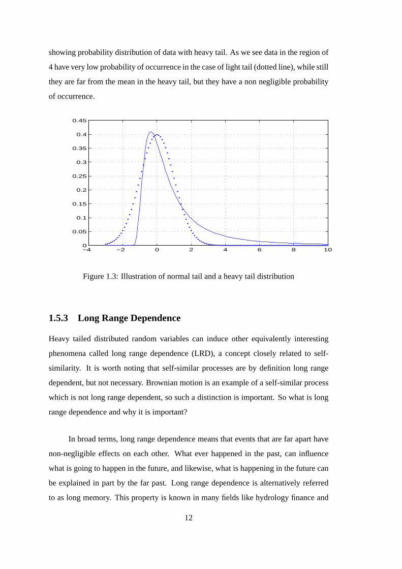
showing probability distribution of data with heavy tail. As we see data in the region of

4 have very low probability of occurrence in the case of lighttail (dotted line), while still

they are far from the mean in the heavy tail, but they have a nonnegligible probability

of occurrence.

−4 −2 0 2 4 6 8 100

0.05

0.1

0.15

0.2

0.25

0.3

0.35

0.4

0.45

Figure 1.3: Illustration of normal tail and a heavy tail distribution

1.5.3 Long Range Dependence

Heavy tailed distributed random variables can induce otherequivalently interesting

phenomena called long range dependence (LRD), a concept closely related to self-

similarity. It is worth noting that self-similar processesare by definition long range

dependent, but not necessary. Brownian motion is an example of a self-similar process

which is not long range dependent, so such a distinction is important. So what is long

range dependence and why it is important?

In broad terms, long range dependence means that events thatare far apart have

non-negligible effects on each other. What ever happened in the past, can influence

what is going to happen in the future, and likewise, what is happening in the future can

be explained in part by the far past. Long range dependence isalternatively referred

to as long memory. This property is known in many fields like hydrology finance and

12

others.

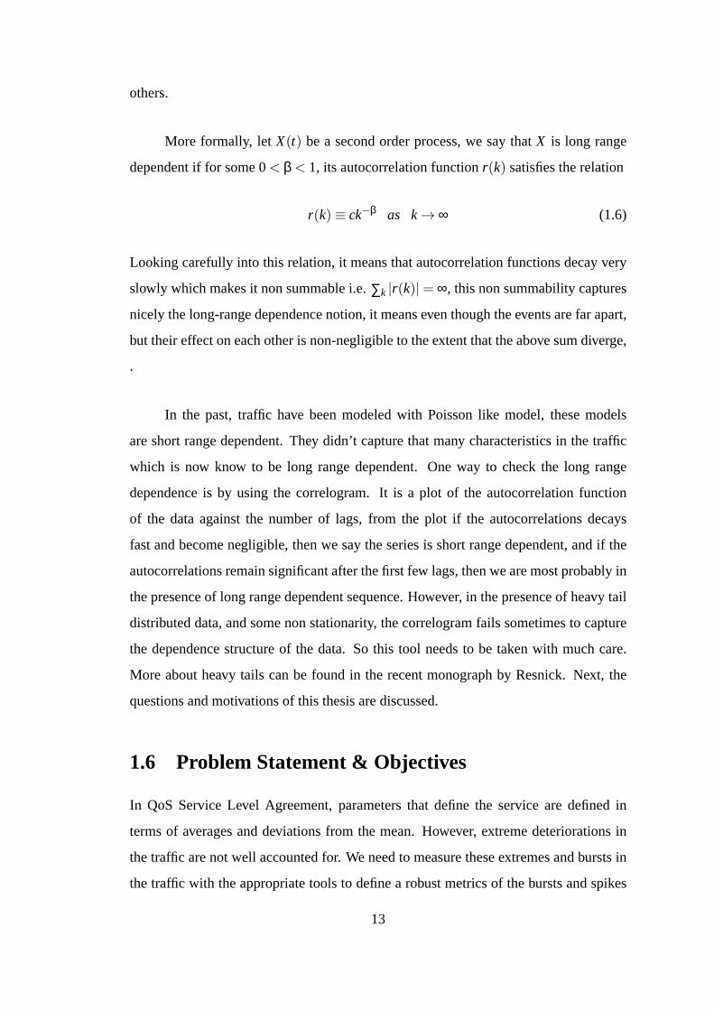
More formally, letX(t) be a second order process, we say thatX is long range

dependent if for some 0< β < 1, its autocorrelation functionr(k) satisfies the relation

r(k)≡ ck−β as k→ ∞ (1.6)

Looking carefully into this relation, it means that autocorrelation functions decay very

slowly which makes it non summable i.e.∑k |r(k)|= ∞, this non summability captures

nicely the long-range dependence notion, it means even though the events are far apart,

but their effect on each other is non-negligible to the extent that the above sum diverge,

.

In the past, traffic have been modeled with Poisson like model, these models

are short range dependent. They didn’t capture that many characteristics in the traffic

which is now know to be long range dependent. One way to check the long range

dependence is by using the correlogram. It is a plot of the autocorrelation function

of the data against the number of lags, from the plot if the autocorrelations decays

fast and become negligible, then we say the series is short range dependent, and if the

autocorrelations remain significant after the first few lags, then we are most probably in

the presence of long range dependent sequence. However, in the presence of heavy tail

distributed data, and some non stationarity, the correlogram fails sometimes to capture

the dependence structure of the data. So this tool needs to betaken with much care.

More about heavy tails can be found in the recent monograph byResnick. Next, the

questions and motivations of this thesis are discussed.

1.6 Problem Statement & Objectives

In QoS Service Level Agreement, parameters that define the service are defined in

terms of averages and deviations from the mean. However, extreme deteriorations in

the traffic are not well accounted for. We need to measure these extremes and bursts in

the traffic with the appropriate tools to define a robust metrics of the bursts and spikes

13

in the traffic. We aim to address these problems and model these extreme behaviors in

the network. These extreme deviations if addressed and modeled properly will provide

better understanding of traffic bursts and spikes which in turn will help define more

robust Quality of Services metrics. In turn, these new metrics will be incorporated into

future service level agreements; which will allow both ISP and users to better manage

SLAs. Users will properly ask the type of services they need and the service providers

will be able to put their valuable resources to whoever actually needs and pays for them.

Our objectives are:

• Enhance the quality of service in the Internet by a proper dimensioning and effi-

cient use of resources.

• Predicting traffic and serious deteriorations in the traffic.

• Creating a clear methodology for the application of Extreme Value Theory in the

field of Internet Traffic Engineering.

Performance evaluation of Internet is a challenge facing network engineers and

is attracting a substantial amount of research work. Our research questions are centered

on:

• How to predict bursts and serious deteriorations in networktraffic?

• What implications does the prediction will have on the Quality of Service con-

tracts (SLA)?

• What metrics should be incorporated into future SLAs to properly account for

the extremes and rare events?

The solution to the first question brings also solution to many other related questions

such as how large the next spike or burst in the traffic will be?what is the probability

of having a large burst in the next time interval?

We want to predict the spikes and serious deteriorations in network traffic parame-

ters such as connection duration, delay, jitter, bandwidthetc.

14

1.7 Thesis Contributions

This thesis contribution can be resumed in the following points:

• Bursts in the traffic are predicted using GEV model based on theblock maxima

approach, where the traffic is segmented into blocks and fromeach block the

maxima are selected for the modeling purpose.

• Bursts are predicted using Generalized Pareto Distributionbased model. In this

case, a threshold is fixed and a GPD model is fitted to all the data above the

selected threshold.

• New Quality of Service metrics are proposed based on the extreme measures

like the Return Level and Return Period, and Mean Excess function. These new

metrics are based on measures from the bursts distribution.

• A clear methodology is developed for the application of the extreme value theory

use in bursts and serious deteriorations prediction case.

• It has been shown that for queues fed with WAN traffic, the behavior of the buffer

will follow Frechet distribution case. Norros has shown analytically that a queue

fed with LAN traffic will follow a Weibull distribution.

The importance of the new QoS metrics implications comes largely from its use in

mission critical applications where there is need for the more robust definition of Ser-

vice Level Agreement. With a robust SLA definition, both users and service providers

are aware of the need of each other and this understanding results in a globally enhanced

quality of service.

Our proposed new models provide the basis from which the new metrics are

defined and extracted.

15

1.8 Scope and limitations

We confine our research work to answer the research questionsin the context of com-

puter networks, and in particular to the Internet. It does not include telecommunication

network like Public Switched Networks, even though some of our techniques still apply

in that context.

The studied traffic is presented in time series quantities like, packet counts, bytes

counts, connection duration, throughput, delay, round time trip etc. The techniques are

applied using the bytes count; however, it can be easily replicated to the other traces

from the above mentioned quantities.

We model bursts and serious deterioration in traffic using Extreme Value Theory

methodology. This methodology is best applied when the parameters to be modeled

have a heavy tailed distribution, i.e they assume very high values frequently far away

from the mean. The heavy tail property of network traffic parameter is a well docu-

mented property [73, 26].

This situation ensures the applicability of EVT methodology. Our treatment fol-

lows such a direction. Our method will apply to parameters such as packet count,

delay, and bandwidth. All of which are well known of being fattailed or heavy tailed.

These specifications happen more in the wide area network traffic (WAN). However,

our method will still be applicable in the local area (LAN) traffic.

Although our method applies to all kind of traffic, if the traffic has a strong corre-

lation factor, our method ceases to apply and some modifications have to be made in

the main theory. However, that is another area of research inwhich the EVT specialists

and mathematicians are into.

16

1.9 Methodology

The next graph shows a block diagram for the methodology thatis going to be used in

the prediction problem. The methodology is based on the Extreme Value Theory. It

starts by collecting data, then chose a proper modeling tehcnique out of three frame-

works. The estimation of parameters is then done. Then, based on the fitted models,

simulation of the bursts and serious deterioration data is conducted. That leads to the

design of performance metrics based on two important measures of return period and

return level. It will be made clearer in in Chapter 3.

The following diagram shows a typical situation where we have more than one

network connected through a common medium, see Figure 1.4. Each network is con-

nected to a boundary node that connects it again to the backbone or the common pool

of resources. These boundary nodes could be routers or intelligent switches. The inte-

rior nodes are the service provider’s routers and network devices. As the algorithm of

Extreme Value Theory is concerned, measurements are applied at the edge boundary

nodes where the traffic shaping can take place. This is where service provider and users

will negotiated the level of service that the user will get and the appropriate metrics to

be included.

1.10 Thesis Organization

After the brief introductory chapter, comes the literaturereview, then methodology,

results and analysis in chapter 4, performance evaluation in chapter 5, and finally the

conclusion. These chapters are arranged as following. Chapter 2 is reserved for the

literature review and assessment. In Chapter 3, the methodology is presented which is

based on the Extreme Value Theory (EVT) comprising three models to be applied. In

Chapter 4, the results are presented and discussed based on the three prediction models.

Chapter 5 is for the prediction and the comparison among the models. In Chapter 6, a

conclusion from this work is drawn.

17

Figure 1.4: Block diagram of the implementation of EVT models

18

CHAPTER 2

LITERATURE REVIEW

In this chapter, literature about basic traffic properties like self-similarity is reviewed

along with its manifestations in different types of traffic (WAN, LAN, HTTP, VBR).

A further look into the origin of self-similarity and its implications is then followed.

Subsequently, bursts are discussed from different angles before narrowing down to the

literature on the proposed methods based on Extreme Value Theory.

2.1 Self-Similarity

A paradigm shift in networking traffic engineering has resulted from a Belcore study in

early 1990s that discovered the self-similarity of networktraffic [58]. In that seminal

work, Leland and colleagues studied in details a state-of-the art high resolution Eth-

ernet traffic data that were collected at Belcore Labs in four sets and contained more

than 1000 million packets. That research is considered a breakthrough in the field of

computer networks. Leland and team members have discovereda ubiquitous property

in the network traffic called self-similarity [28]. They showed in their work that the

Markovian model, largely used for the modeling purposes, does not capture reality, that

the aggregated Ethernet traffic is Self-Similar or fractal in nature. This property means

that burstiness is observed across different time scales and is persistent with the aggre-

gation of traffic. This is in contrary to former beliefs that aggregation has the effect of

smoothing out the bursts and roughness in traffic when it is modeled by Poisson type

models [75].

The degree of self similarity varies from one process to another. Hurst’s parame-

ter is used to measure the degree of self-similarity, ref. This parameter is the exponent

appearing in the definition of self-similar processX(t), we say thatX is self-similar

if it satisfies the relationship{X(at), t ∈ R} ={

aHX(t), t ∈ R}

, wherea is a constant.

The symbolsH in this equation stands for Hurst’s parameter. It assumes its values

between 0.5 and 1. The higher the value ofH, the more pronounced is the degree of

self-similarity. Hurst’s parameterH gets larger with increasing network utilization.

Shortly after the discovery of self-similarity, a lot of research studies were con-

ducted in different contexts and using different datasets as to replicate or check this

new discovered property. In particular, researchers proved the self-similarity in differ-

ent settings like (Wide Area Network, Variable Bit Rate, File Transfer Protocol, and

Hyper Text Transfer Protocol) and replicated the study in different environments.

In 1994, Vern Paxson and Sally Floyd [75] reported similar findings on wide

area traffic. They demonstrated that wide area traffic is self-similar. They analyzed 21

datasets collected from different sources including the Belcore sets. While the TCP

connection arrival for FTP and Telnet behaved as Poisson, the packet traffic or data

during the session deviate remarkably from Poisson distribution. Modeling the traffic as

Poisson resulted in models and simulations that extremely underestimate the burstiness

of the actual multiplexed traffic.

Wide Area Network traffic has also been a subject of further investigations by

researchers. W. Willinger and others have gone one more stepin the modeling of WAN

traffic and showed that it is not only self-similar but it is also multifractal in nature

[33, 82]. Multifractality is richer than the simple self-similarity in properties. And the

self-similarity can be thought of as a special case of the multifractal property. They

fitted multiplicative cascade model to it.

However, the concept of Multifractality has not gone without some controversy.

Patrice Abry and others have challenged the Multifractality suggested by W.Willinger

and others, and described it as weak and overstated [95], butstill they did not provide

evidence against the multifractality. They went on and suggested a point process model.

However, the subject remains controversial. In [92], MuradS. Taqqu and others tried to

20

answer the question of whether the network traffic is self-similar or multifractal. They

gave some insight into the question and acknowledged that LAN/WAN traffic can be

modeled by either self similar or multifractal models and yet, there is no clear cut in the

modeling and the question remains open, giving opportunityfor physically motivated

network models. Meanwhile, other research directions havetaken place to show the

self-similar property in other types of traffic like the Variable Bit Rate (VBR) traffic

and the World Wide Web traffic (WWW) as well.

For VBR video traffic, M. Garett and W. Willinger studied VBR video traffic and

reported the result in [39]. They studied the VBR video trafficcarefully to better un-

derstand the bandwidth process. They applied a simple intra-frame video compression

code to an action movie, they showed that the VBR video traffic is long-range depen-

dent (LRD), a property that is closely related to the self-similarity. Another property

being reported is the heavy-tailed marginal distribution of the information content per

time interval. In another study, Jan Beran and others have come to a similar conclu-

sion using a variety of different codec in the VBR video data, see [48]. They showed

that video transmission exhibits self-similarity. They studied varying lengths of video

frames and found that it is better fitted to a Pareto distribution, especially in the upper

tail. These characteristics of the VBR video are inherent regardless of the codec cho-

sen or the scene itself. It should also be clear by now that when we talk about Pareto

distribution it means distribution with heavy tails, a property that is demonstrated to be

closely related to self-similarity [79].

Within the context of the world wide web traffic (WWW), M. Crovella, A.Bestavros

and others have proved the self-similarity of the world wideweb traffic as well, [23].

They modeled browsers using an ON-OFF model, where ON periodcorresponds to ac-

tivity or transmission and OFF is the non-activity. They found that ON-periods follow a

Pareto distribution. Meanwhile, Martin F. Arlitt and others have done a thorough analy-

sis on different datasets of Web server workload, [5]. They came to the conclusion that

Web traffic is self-similar most of the time with different self-similarity parameter de-

pending on the context and that the heavy tail distribution of files in web is the biggest

21

contributing factor to the observed self-similarity. Theyalso identified ten work load

invariants (observations that apply across all the data sets studied).

With the emergence of Voice over Internet Prtocol (VoIP) communication, VoIP

traffic also has gone self-similarity investigations, and it is found that it complies with

self-similarity concept, [76] and [16]. In [16], using realtime data from VoIP calls, the

analysis was done on the aggregated traffic capturing two main metrics, the interarrival

times of consecutive VoIP packets and the throughput of the aggregated traffic, estima-

tion of Hurst’s parameter is found in the range between 0.7< H < 1, which is a strong

indication of the self-similarity.

The self-similarity of the traffic is now clearly established, but it is not without

some resistance from researchers who still believe in the earlier non self-similar models

[17]. However, that controversy is likely to be confined in very specific settings and

diminish in front of the more established fact of self-similarity. Natural questions would

be: what are in the origin of the self-similarity of network traffic? and what effects does

this have on performance?

2.2 Origins of self similarity

Walter Willinger et al. provided physical explanation to the observed self-similarity of

the traffic, [102]. They showed the origin of the self-similarity through a reformulation

of an ON-OFF model originated from Mandelbrot’s work in [64], where ON period cor-

responds to transmission period and OFF to a non transmission period. Inspired by the

packet train model of Jain and Routhier [47], they assumed that individual sources send

packets to the network through an ON-OFF mechanism where ON periods correspond

to sending of a packet while OFF period is for a silence period.

In contrast to traditional modeling where ON-OFF periods are understood to be

exponentially distributed, it is found that at least ON- or OFF-period is heavy-tail dis-

tributed (Noah effect). The heavy tailed distribution, sometimes called infinite variance,

of ON-OFF period means literally that activity/silence periods can be very long and it is

22

so frequently. The superposition of the individual ON-OFF traffic source produces the

self-similar traffic property (Joseph effect). This physical explanation applies to LAN

traffic and in large extent to the WAN traffic also. These ON-OFF periods are strictly

alternating and have distributions with heavy tail. However, this heavy tail property is

present in many Internet traffic parameters like files sizes,transmission duration pack-

ets count or bytes count per time interval. Numerous studieshave proved the presence

of heavy tail in these quantities in Internet traffic, examples are [58], [101], [100], in

particular, for the heavy tail in file size see [5] and [78], for transmission rates and

durations see [65] and Resnick article in [34].

The long range dependence is closely related to self-similar property in the Inter-

net traffic. Long range dependence is found in many quantities related to the traffic as

well, variable bit rate video is such an example [48].

The effect of self-similarity on performance is widely studied. It may include a

profound impact on the network parameters like delay, jitter and packet loss[73]. These

effects can be understood since the Markovian models underestimate the burstness of

the traffic and even suggest that the traffic get smoother withaggregation which is not

the case [84].

Knowing the model is a part of the story, the other part is to determine param-

eters’ values of the supposed model which can be done by estimation. In general,

fewer model parameters are preferred to many, this is calledparsimonious modeling.

Self-similar models are parsimonious since they have one parameter that uniquely de-

termines the process called Hurst’s parameter.

A number of methods are used to estimate the value of Hurst’s’s parameter, they

range from analysis of variance of the aggregated traffic, the rescaled range R/S method,

Whittle estimator, and recently wavelet based one [1]. The analysis of variance method

relies on the slowly decaying variance of the self similar processes. The variance of

the aggregated process is plotted on log-log scale and from the slope of the plot the

parameter H is determined. The other promising method is theR/S statistics method.

23

R/S statistics is the ration between partial sums of deviations of observations from their

mean to their standard deviation. Hurst found that this quantity obeys some empir-

ical relationship that includes H. The H parameter can be estimated by plotting that

empirical relationship in a log-log plot.

A rescaled variance method is also been proposed [15]. The rescaled variance

method V/S is similar to the R/S method. It uses the sample variance in the place of the

mean in the R/S method. V/S method is superior to R/S in some cases specially when

H’s true value is around 0.5 .

Patrice Abry and Darly Veitch derived an estimator of the degree of self-similarity

H using the wavelet method [1]. They showed that the estimatoris unbiased, consistent

and have the lower Cramer-Rao bound [41]. More interesting, itis shown in that work

that wavelet estimator is rigorous with respect to trends, weather these trends are linear

or polynomial. In addition, it gives a practical way to eliminate the effect of trend on

the estimator by varying the number of vanishing momentsN of the analyzing wavelet.

For a recent survey of the estimating methods, see [81].

2.3 Bursts in the traffic

In [75], bursts have been implicitly defined as a connection duration above a given

threshold and was applied to different types of traffic, it was referred to as http bursts,

ftp burst, telnet bursts etc. In [109], and a series of other related publications by the

same authors, bursts have been defined in data streams to be anunexpectedly large

number of events occurring within some certain measurement(time), it is a general

definition which the authors apply to all kind of events from social to hurricanes and

floods as a part of a knowledge discovery approach using some specific data structure.

The same point of view is also shared by [111], in which burstsare defined as abnormal

aggregation in data streams. In telecommunication and datatransmission networks,

bursts are referred to differently as a continuous transferof data from one source to

another without interruption [63]. Another cluster of literature is referring to burst as a

24

threat to network and is dealing with bursts as an anomaly in the network traffic rather

than a property of the traffic [66, 107, 32].

These disagreements in bursts definition make the task of coming with a defi-

nition that satisfy all these requirements a difficult one, it is even made worse by the

broad implementation of the word bursts in differently seemingly unrelated disciplines.

One way to digest all these seemingly non-consistent definitions is to look at bursts as

an attribute rather than an object, so a notion of Bursty traffic and bursts in the traffic

can be both valid. In this research some definitions of the bursts will be agreed on for

the purpose of this study.

In the following, bursts are defined as unusual high aggregation of data in a rel-

atively small time window. It may be adapted in two differentways when the EVT

based models are suggested in later chapters, in the block maxima, bursts are defined

to be the block maxima taken in a predefined intervals that canbe minutes, 10 minutes,

etc., while in the peaks over threshold, bursts are defined tobe all the data above a

given threshold. These implementations of bursts definition are in the best interests of

the QoS perspective to measure, quantify and propose SLA agreements that take into

account measures of bursts and extreme deteriorations.

As varying as their definitions are, bursts have been studiedfrom different per-

spectives. For instance, and from security perspective, bursts mean a possible threats or

attacks to the network, [66, 107, 32]. Networks need to be monitored and bursts need to

be detected so that attacks can be repelled on time, this is true for the intrusion detection

and the intrusion prevention mechanisms. In [110], researchers detect burst for online

monitoring of data streams, which can be applied to network traffic as well as for trend

analysis, intrusion detection and geophysical applications and web clicks analysis. An

inverted Histogram (IH) has been used to adaptively detect bursts in data streams and

in particular the double sided bursts (increasing - decreasing) without being affected

by the frequent bumps in the data [110]. Many other methods are being used for de-

tecting bursts or aggregation of data. We call in particularly those with application to

email [54], to gamma ray [111], in network traffic [22]. In [90] and using the notion of

25

compact summaries, authors tried to detect abnormal changes in the traffic. In [109],

authors used Shifted Binary Tree and a heuristic search algorithm to detect burst across

multiple window sizes.

Wavelets methods have also seen their application to detectbursts and anomalies

in networks. Wavelet analysis is an ingenious form of transformation that is closely

related to the Fourier transformation, where instead of representing the data in the usual

time domain, data are transformed into the frequency domain[62]. A shortcoming

of Fourier transformation is that all the information abouttime is lost once the data

(signal) are transformed into the frequency domain. However, wavelet transformation

or analysis, by using different kind of transformation, retains the frequency as well

as the time, thus it transforms the signal into the frequencydomain while retaining

information about the time. The resulting wavelet coefficients constitute in themselves

a new time series that can also be subjected to research and observation.

Many publications have used the wavelet method with varyingdegrees of suc-

cess in detecting the bursts in traffic, in particular in [59,18, 106, 105]. In [59], burst

and anomalies in the traffic caused by distributed denial of service attack (DDoS) are

detected using energy distribution based on wavelet analysis. The detection algorithm

is based on the traffic behavior analysis. Energy distribution of the normal traffic is

calculated, when a sudden change in the energy level appears, that means an anomaly

in the network and hence a possible threat to the network. Authors in [18] used wavelet

techniques to analyze the traffic and detect if a sudden change in the rate of arrival

happens then it would be concluded that an attack or a threat to the network is emi-

nent. Many other studies used the wavelets to detect threatsor attacks in the network

using bursts as a commensurate to an anomaly, see [106, 105].Since there are many

types of wavelets, the choice of wavelet has also presented another set of challenges to

researchers, however, without delving too much into the details and since bursts here

are used from security point of view which is not really the concern here, a point of

reference would be sufficient, see [77].

26

On the other hand, when bursts are defined as very high aggregation of traffic in

small time interval, it does not necessary indicate a threat, it could be seen as spikes

and serious deterioration in the traffic. Instead of only detecting the bursts, a more

proactive approach would be to predict thesebursts which isthe central theme of this

thesis. As Internet is becoming the global infrastructure for business and all other types

of modern communication, these kind of bursts may cause hugelosses and damages if

not managed outside of the historical best effort architecture of the Internet to provide

the agreed on service.

2.4 Quality of Service (QoS)

Historically, Internet was organized to provide the best effort services, i.e. applications

will send their traffic into the Internet in the hope that theywill arrive to the receiving

station. No guarantee of delivery from the part of the Internet. Take the example of

two typical users, one is sending an important email and the other is surgeon operating

a distance open heart surgery. Both of them rely on the networkto deliver. A delay

of seconds in the network will be barely noticed by the first user (email sender). The

same delay if happened to the surgeon will be fatal, or at least so to the patient. Such a

situation shows clearly that different users have different expectations and requirements

from the network service and also have different levels of tolerance to delays and inter-

ruptions. This best effort Internet is no longer feasible intoday’s environment where

Internet is becoming the infrastructure for business transactions, communication, and a

lot more, [55].

Quality of Service becomes an important concept in the Internet today; two ap-

proaches for the quality of service are prevalent in the literature, integrated services

and differentiated services. A study that was supported by the Internet Engineering

Task Force presented a compelling discussion about the needfor integrated services,

see [12]. In integrated services, before the traffic is sent,the application will signal its

requirement and ask for reservation of some resources, the traffic is only sent when the

resources required are available; this mechanism is calledresource reservation setup

27

protocol (RSVP), for the design and more about this algorithm, the reader is referred

to [108]. Thus, Integrated Services is very effective and efficient method in provid-

ing Quality of Service solutions in the Internet; however, it is more effective in single

managed networks, and when it comes to scalability it suffers [96].

A most common and scalable approach is the differentiated services approach, it

lies somewhere between the best effort Internet and the integrated services. In differ-

entiated services traffic is classified into classes called forwarding classes and allocates

resources based on the traffic class, which means each class of traffic is treated differ-

ently giving high priority to some and low priority to others[11]. When packets arrive

at network, it performs packet classification and traffic conditioning.

Network services in the case of differentiated service are defined and agreed on

between the Internet service provider and the customer, where all the parameters of the

service are formally defined in a legally binding contract called service level agreement

(SLA). SLAs are a subject of constant change and modifications to reflect the needs of

both the service providers and the users, many mechanisms are there for the negotia-

tion of these agreements, a recent approach is using Agents for a completely automated

negotiation for the service, see [104]. Associated with SLAcomes the traffic condi-

tioning agreement TCA where technical details of the serviceparameters are formally

defined. Thus performance metrics are included in the SLAs like throughput, delay,

jitter, average connection duration and others. However, parameters that determine the

class of services are defined in terms of average and deviation from the means, thus,

extreme deteriorations in the traffic are not properly addressed. Since it is noted earlier

that Internet traffic variables exhibit heavy tail property, more appropriate methods to

quantify and measure the extremes is thus needed.

2.5 Extremal Events : History and Motivations

Netherlands is the country where most of the early motivations behind extreme value

engineering took place. This country has more than a third ofits surface below the sea

level. The danger of floods and high see levels is thus obvious. The government has to

28

tackle this problem and protect its territory by building high dikes. The natural question

to be asked is how high these dikes are to be built so that the probability of floods is

very small? The government requirement for this ”very small” probability is 0.0001

for any given year. Another question of equal interest is howhigh these dikes are to be

built so that a certain very high sea level can be expected once in a hundred or thousand

year period?

These questions posed enormous challenge for engineer at that time. They had no

direct answers to these questions using the classical statistical theory. The seemingly

difficulty comes from the need to extrapolate beyond the available data. Extreme Value

Theory was thus the right tool.

The analogy between the Netherland dike problem and internet traffic bursts and

serious deteriorations is thus clear. Both of the events if happened might have profound

unwanted effects on the system. Prediction and modeling of these rare, hence frequent

events is thus important. However, before going into the details of the theory a brief

account of the history of Extreme Value Theory is in order.

The beginning of Extreme Value Theory development can be dated back to 1928

when Fisher and Tippet derived a key result for the possible law limits for sample max-

ima [36], but the idea itself can be traced back as far as 1709 when Nicolas Bernoulli

discussed the mean of the distribution of the largest distance in some given settings.

The probabilistic side of the theory was treated by R. von Mises (1936) leading

to the comprehensive work of B. Gnedenko (1943). The statistical side of extremes is

treated by J. Pickands III(1975). A comprehensive reference manual for the theory was

published on 1958 and authored by E. J. Gumbel.

In the last two decades, we noticed more publications than ever and a growing

interest in the theory by practitioners and engineers from different disciplines. Em-

brecht and others published a manual detailing the applications of extreme statistics

to the Insurance and Finance industry[29]. We notice among others Jan Berlian and

29

others in ”Statistics of Extremes”, [8]; Enrique Castillo and others in ”Extreme Value

and Related Models with Applications in Engineering and Science”,[19]; a collection

of research papers is edited by Barbel Finkenstadt and HolgerRootzen titled ”Extreme

Values in Finance, Telecommunications and the Environment”, [34]; Stuart Coles pub-

lished a monograph titled ”An Introduction to Statistical Modeling of Extreme Values”

in which he addressed the essential of the theory for its application in different field[21].

The literature of Extreme Value Theory is huge, however, we selected a representative

body of the literature of the theory and it is by no means a complete account of the

subject, which is out of the scope of this brief introductory.

Generally speaking, to find the distribution function of anyrandom variableX

we would write

F(x) = P(X < x) (2.1)

whereF is the distribution function andP stands for probability function. The distri-

bution function takes value strictly between 0 and 1, i.e 0< P(X < x) < 1; The same

applies for the random variableMn (The maximum of random samples).

To calculate its distribution function one would writeG(x) = P(Mn < x). And since we

know thatMn = Max(X1,X2, . . . ,Xn) the above expression can be re-written as

G(x) = P(Mn < x) = P(Max(X1,X2, . . . ,Xn)< x) (2.2)

The eventMax(X1,X2, . . . ,Xn)< x is equivalent to the event(X1 < x,X2 < x, . . .Xn < x).

Substituting in the above expression and noting that the probability of the intersection of

independent events equals the multiplication of their probabilities, the above expression

transforms to

G(x) = P(X1 < x)∗P(X2 < x)∗ . . .∗P(Xn < x) = [F(x)]n (2.3)

So this way we found the distribution function of the maxima of random samples

G(x) = [F(x)]n. However, sinceF(x) < 1, the distribution function will degenerate

to 0 asn gets larger and larger. This will make difficult and worthless result to do with.

30

This is exactly why we needed more rigorous result for the distribution of the maxima

of random samples. And this is exactly what brought the Extreme Value Theory into

being, a field of knowledge that is pioneered by the work of twoprominent scientists,

Fischer and Tippet [37].

Two methods are commonly implemented from EVT. The first and most com-

monly used is the Block Maxima in which data are segmented intoblocks and the max-

ima are taken from each block and a new series of maxima is constituted. A model is

thus fitted to this new series of maxima. The second method is the Peaks Over Thresh-

old method, in this second a threshold is fixed and data above that threshold are fitted

to a distribution.

An extension of the extreme value models is the r largest order statistics model.

In contrary to what happens in block maxima method were only the maxima is chosen

from each block, in r largest order statistics and as the namesuggests, from each block

the r largest values are chosen to be modeled instead, wherer > 1. The joint distri-

bution of the r largest value is then defined and used to calculate the parameters that

correspond to the GEV for the block maxima. This method is considered as a middle

way between the POT and the BM methods, its development can be attributed to the

work of Weissman in[99]. The monograph by Stuart Coles provides detailed discussion

as how about to implement the r largest order statistics model in practice [21].

Another research direction which is more theoretical is done by Albin, [3] and

[4]. Albin showed the existence of limit distribution for maxima from self-similar pro-

cesses. In his highly abstract mathematical work, he derived upper and lower limits for

the distribution of maxima of self-similar processes including classes of totally skewed

alpha stable processes. This work gives us the confidence of the applicability of the

theory to the self-similar network traffic. However, the only concern is that Albin work

is a very much mathematical with no clear indication of how about to apply the theory

in practice. It is highly theoretical and inaccessible to the casual practitioner.

31

2.6 Traffic Prediction

Predicting Internet traffic in particular proved to be a challenging task due to the self-

similarity of the traffic and its long range dependence. In [103], decomposition is used

to predict bursts and serious deteriorations in the traffic.The essence of the method

lies in the use of filters and a variant of Least Square Method.Firstly, the traffic is

decomposed into two parts, low frequency and high frequency. Then both the low and

high frequency traffic are predicted using a variant of leastsquare method. The result

of the prediction is then superposed back to produce the predicted traffic. The main

motivation behind that work is to predict possible attacks or threats to the network.

Several other attempts have been and continue to be made to model bursts. Researchers

in [9] reviewed bursts and other related facts like long range dependence and heavy

tails, termed stylized facts and fitted an analytical model to the bursts in the data traffic.

They modeled bursts and related quantities by an infinite source Poisson model. In this

analytical model, they took measurements in a fixed time windows delta and let this

delta goes to zero to capture bursts. It is a slight modification of the queuing system of

infinite source Poisson model.

Although extreme value theory methods have been in practicein a number of

discipline for decades, their introduction into the field oftraffic engineering is rela-

tively recent, in [34] Sidney Resnick argues for the use of Extreme Value Theory for

the telecommunication paying a particular attention to theinherent properties of the

telecommunication data network like heavy tails and long range dependence, Resnick

made it clear that although some models may fit some data, but the challenge would

remain which classes of model would fit which classes of data.Resnick in [34] gave

an insight into some questions related to modeling data networks using a variety of

tools from statistical analysis, in particular, plots likequantile to quantile plot, Hill’s

plot, mean excess plots are being discussed to check on the heavy tail and long range

dependence of the data. When it comes to extremes, Resnick touched briefly on the ap-

plication of the extreme value theory paradigm and in particular the peaks over thresh-

old method but in very broad terms with an open end questions.A number of other

32

studies suggested EVT as a framework for modeling differenttypes of traffic [94, 60].

In [94], Masato Uchida used the throughput as a network parameter to be modeled. It

was argued that throughput, link usage rate, packet loss rate and delay time can be used

to predict telecommunication quality. To arrive at predicting serious deteriorations in

telecommunication quality, POT method was used for the modeling by fitting a gener-

alized Pareto distribution for the purpose. The data was divided into two sets, on set

is considered unknown while the other set is used to construct the model, the model is

used to predict the supposedly unknown set. He showed that the POT using GPD is bet-

ter in approximating the unknown part of the data than the previously commonly used

lognormal distribution. In [60], authors used the same method POT for the analysis of

wireless traffic. They fitted a GPD model and reported the improvement to their model

compared to the lognormal, Gamma, Exponential, etc. The computational overhead is

clearly reduced when using the EVT model because we need onlya subset of the data

to work on.

A passage in the literature to the extreme value traffic engineering was in an arti-

cle by RATZ. The article (and the references therein) discusspeak traffic in telephone

switching office and fitted a gamma distribution to it. Although the word extreme value

was mentioned, it referred to a different thing than EVT. They used the extreme value

to mean literally the maximum value of telephone traffic in a given setting, while we

use it to denote a theory. Moreover, they used and fitted not anEVT distribution, but a

gamma distribution to predict peaks in the traffic correctly. The research in [68] gave

an overview of some of testing procedures to determine the distribution of the extremes

and to assess EV conditions. They illustrated some of the recent testing tools using

teletraffic data.

In [52], systems downtime or repair times are being studied for their obvious

importance in planning and it was found that system repair time follows a heavy-tailed

distribution. Since the mean fluctuates too much (not existent) and thus cannot be used

as metric to evaluate the system performance, a concept called T-year return level from

Extreme value theory is used for the analysis and prediction. The T-year return level,

33

which is the amount exceeded once in a T-year return level, isused as way to predict the

down time or IT repair time. This same return level is used in finance literature and is

referred to as Value at Risk (VAR). As reported there, the mean is not a robust metric to

be considered in the heavy tail distributed parameter considered. The T-year return level

is used instead. The method is clearly described and its application is straightforward,

however, the study did not include any evaluation of the performance of the prediction

results. This study could be improved by including the return period which is the time at

which certain threshold will be reached. As remarked, very few these studies that touch

on the application of the extreme value theory, these studies applied the theory of EVT

and in particular the POT method with the assumptions that itholds true. They did not

include any preliminary analysis of the data to check whether the theory assumptions

hold or not, such steps are important and crucial for the success of the model. One of

the most important reasons for this is the i.i.d. assumptions. The theory was developed

based on this assumption. As it is shown in [57], if data are highly dependent then the

application of theory needs to be modified and a further parameter called extremal index

need to introduced, otherwise erroneous results would be produced. In this regard,

we can say that the literature survey so far found that in applying EVT in network

traffic was superficial and is ignoring the high dependence structure of the traffic where

extremal index assumes a major role in correctly modeling the data. This might be the

result of the recondite nature of the theory itself, but nevertheless, it is an important

step in the prediction of bursts and serious deteriorations.

2.7 Summary

In this chapter, we discussed the subject from its widest aspect and narrowed down

to the problem. We started by the Self-Similarity literature, its existence in different

types of traffic and some of the controversy surrounding the self-similarity. In the

subsequent sections, we looked into the bursts definition from different angles in the

literature before positioning and defining our concept of the bursts. In the later part we

reviewed our methodology, Extreme Value Theory and some of it to other disciplines

and problems.

34

CHAPTER 3

EXTREME VALUE THEORY BASED MODELING

This chapter presents the theory behind the methodology that is applied for bursts and

serious deteriorations prediction problem. It starts by showing a system model, and then

introduces the cornerstone theory. Three models based on the theory are introduced

along with concepts of Return Level and Return Periods that areproposed as metrics

for Service Level Agreements. Model diagnostics and simulation techniques based on

EVT are also discussed.

3.1 Traffic Bursts & Serious Deteriorations

Network traffic parameters like connection duration, packet count, file size, bytes count

share properties like heavy tail, long range dependence, and burstiness. Understanding

these properties and their implications is central to the proper modeling and prediction

of bursts and serious deteriorations in the traffic [79].

Bursts and serious deteriorations of different traffic quantities are bound to hap-

pen and they are unavoidable [9]. Their prediction and proper quantification with ade-

quate measures will define robust Quality of Service (QoS) metrics to be incorporated

into future QoS service level agreements. This will be done in terms of probability

density distributions and the tools derived from them.

While central limit theorem (CLT) states the limiting distribution of sample means

when the number of trials increases [35], the extreme value theory (EVT) is about the

limiting distribution of sample maxima. The CLT defines the normal distribution as the

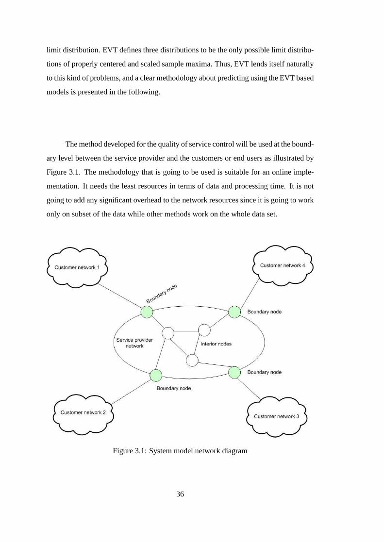
limit distribution. EVT defines three distributions to be the only possible limit distribu-

tions of properly centered and scaled sample maxima. Thus, EVT lends itself naturally

to this kind of problems, and a clear methodology about predicting using the EVT based

models is presented in the following.

The method developed for the quality of service control willbe used at the bound-

ary level between the service provider and the customers or end users as illustrated by

Figure 3.1. The methodology that is going to be used is suitable for an online imple-

mentation. It needs the least resources in terms of data and processing time. It is not

going to add any significant overhead to the network resources since it is going to work

only on subset of the data while other methods work on the whole data set.

Figure 3.1: System model network diagram

36

3.2 Extreme Value Theory

Fisher and Tippet theory is considered the fundamental theory in Extreme Value Theory

literature [29]. Our methodology depends primarily on results derived from this theory.

This theory serves for the sample maxima as does the central limit theorem to the

sample means. It defines the only three possible limits of properly centered and scaled

maxima of observations.

Say we have a series of random variablesX1,X2, . . . ,Xn. This sequence of random

variables can represent any event we are interested in such as packet count, bytes count,

bursts, file size, or connection duration. We suppose that these random variables are

independent and identically distributed (i.i.d.) with a common distribution functionFX.

Now take the maximum of samples of random variablesMn = max(X1,X2, . . . ,Xn) and

constitute a new series of random variablesMn. To calculate the distribution of these

Mn, we could have

FM(x) = P(Mn < x)

= P(X1 < x,X2 < x, . . . ,Xn < x)

= P(X1 < x)∗P(X2 < x)∗ . . .∗P(Xn < x) = [P(X < x)]n. (3.1)

Assuming that a probability function takes values between zero and one, this last

expression will converge to zero asn gets larger, making it of little or no use. EVT

solves this problem and tells us about the limiting distribution of these maxima.

Theorem 1. (Fisher-Tippet[37, 29]). Let(Xn) be a sequence of independent identically

distributed random variables with distribution FX. Let Mn = max(X1,X2, . . . ,Xn). If

there exist norming constants cn > 0 and dn ∈ R and some non-degenerate distribution

function H such that

Mn−dn

cn→ H (3.2)

then H is one of the following three types:

37

• I (Gumbel, [42])

Λ(z) = e−e−( z−ba )

, z∈ R (3.3)

• II (Frechet, [38])

Φ(z) =

0, z≤ b

e−( z−ba )−α

, z> b

(3.4)

• III (Weibull, [97])

Ψ(z) =

e−(−( z−ba )α), z< b

1, z≥ b(3.5)

These three distributions are the only possible limit distributions for properly centered

and scaled maxima [37, 19]. Furthermore, we say thatF is in the maximum domain

of attraction (MDA) of one of the above distribution if the maxima from sample from

F converge to that distribution. For example, we writeF ∈ MDA(Ψ) if maxima drawn

from F converge to a Weibull distribution, denotedΨ.

These three distributions are shown in Figure 3.2. They havedifferent shapes

and imply different properties. We find the Weibull distribution to be of a finite upper

tail which means data that can be fitted into this calls of distributions are bounded from

above. On the other hand, the Frechet distribution shows a heavy tail distribution with

an unbounded support which clearly shows the tendency of data fitted to this distribu-

tion to assume very high values frequently. The Gumbel distribution lies somewhere in

the middle between the two distributions, Weibull and Frechet. Both Frechet and Gum-

bel densities are skewed to the right, while the Weibull density is skewed to the left.

All the three distributions have scale, location, and shapeparameters except Gumbel

which has no shape parameter. More discussion about the different properties of the

three extreme value distributions can be found in [19].

Thus, EVT outlines the only possible limits for the distribution of the maximum

of random samples. The proof of this theory is rather technical; Interested readers can

38

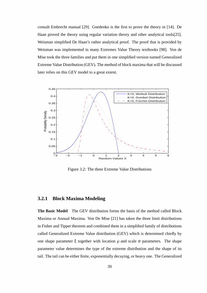
consult Embrecht manual [29]. Gnedenko is the first to prove the theory in [14]. De

Haan proved the theory using regular variation theory and other analytical tools[25].

Weisman simplified De Haan’s rather analytical proof. The proof that is provided by

Weisman was implemented in many Extremes Value Theory textbooks [98]. Von de

Mise took the three families and put them in one simplified version named Generalized

Extreme Value Distribution (GEV). The method of block maxima that will be discussed

later relies on this GEV model to a great extent.

−3 −2 −1 0 1 2 3 4 5 60

0.05

0.1

0.15

0.2

0.25

0.3

0.35

0.4

0.45

Random Values X

Prob

abilit

y Den

sity

K<0, Weibull DistributionK=0, Gumbel DistributionK>0, Frechet Distribution

Figure 3.2: The three Extreme Value Distributions

3.2.1 Block Maxima Modeling

The Basic Model The GEV distribution forms the basis of the method called Block

Maxima or Annual Maxima. Von De Mise [21] has taken the three limit distributions

in Fisher and Tippet theorem and combined them in a simplifiedfamily of distributions

called Generalized Extreme Value distribution (GEV) whichis determined chiefly by

one shape parameterξ together with locationµ and scaleσ parameters. The shape

parameter value determines the type of the extreme distribution and the shape of its

tail. The tail can be either finite, exponentially decaying,or heavy one. The Generalized

39

Extreme Value (GEV) distribution function is given by

Gξ,µ,σ (z) =

e

{

−(1+ξ( z−µσ ))

− 1ξ}

i f ξ 6= 0

e{−e−(z−µ)/σ}, i f ξ = 0

(3.6)

defined on{z : 1+ξ(z−µ)/σ > 0} where both shape parameterξ and location param-

eterµ take values in the real line. However the scale parameterσ is always greater than

zero. The parameterξ determines the shape of the distribution. Whether the distri-

bution has a light tail or heavy tail depends on the value and sign of this parameter. If

the parameterξ < 0, GEV family is referring to Weibull distribution which hasa finite

support, to Frechet distribution forξ > 0, and to Gumbel in caseξ = 0. One should

note that we are talking about the distribution of the maximum of the samples and not

the whole data, a concept that is frequently misunderstood.

BM Method Block Maxima (BM) is the classical approach to model extremes;it

works by dividing data into blocks, then from each block takeonly the highest value

which is the maximum [8]. Figure 3.3 illustrates the use of this method where data are

segmented in blocks. From each block the maximum value is selected. These maxima

constitute a new series composed solely of sample maxima where sample here refers

to a particular block. A GEV distribution is then fitted to this new series of maxima by

estimating its parameters.

Let’s say we have a trace of data in the form ofX1,X2, . . . ,Xmn, with X represent-

ing the packet count or any other quantity of interest (connection duration, packet size)

andm,n are integers. To implement the method, first we divide this series of raw data

into madjacent blocks, each with sizen. The choice of the block sizen should be large

enough so that the theory is valid to be applied on the new series of maxima, given by

M( j)n = max(X( j−1)n+1,X( j−1)n+2, . . . ,X( j−1)n+m) f or j = 1, . . . ,m (3.7)

40

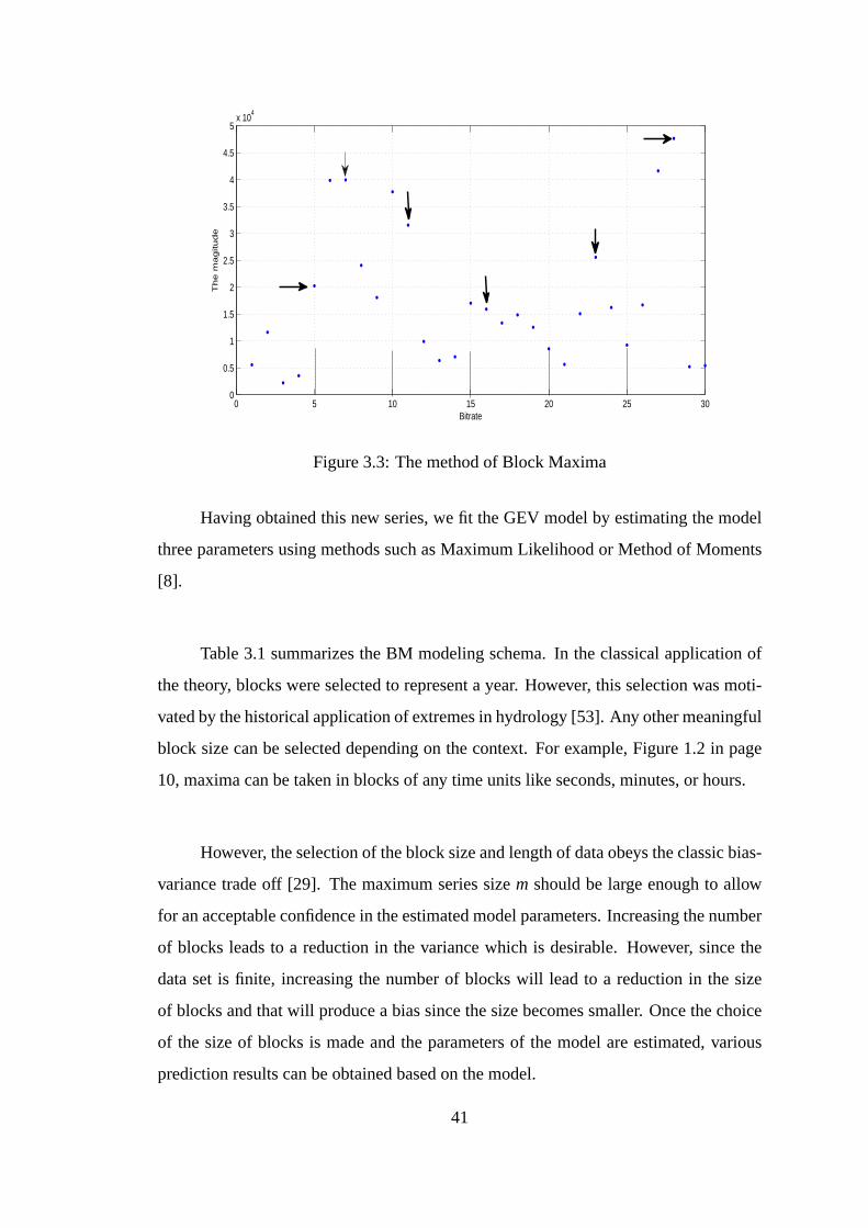
0 5 10 15 20 25 300

0.5

1

1.5

2

2.5

3

3.5

4

4.5

5x 10

4

Bitrate

Th

e m

ag

itu

de

Figure 3.3: The method of Block Maxima

Having obtained this new series, we fit the GEV model by estimating the model

three parameters using methods such as Maximum Likelihood or Method of Moments

[8].

Table 3.1 summarizes the BM modeling schema. In the classicalapplication of

the theory, blocks were selected to represent a year. However, this selection was moti-

vated by the historical application of extremes in hydrology [53]. Any other meaningful

block size can be selected depending on the context. For example, Figure 1.2 in page

10, maxima can be taken in blocks of any time units like seconds, minutes, or hours.

However, the selection of the block size and length of data obeys the classic bias-

variance trade off [29]. The maximum series sizem should be large enough to allow

for an acceptable confidence in the estimated model parameters. Increasing the number

of blocks leads to a reduction in the variance which is desirable. However, since the

data set is finite, increasing the number of blocks will lead to a reduction in the size

of blocks and that will produce a bias since the size becomes smaller. Once the choice

of the size of blocks is made and the parameters of the model are estimated, various

prediction results can be obtained based on the model.

41

Table 3.1: Summary of Block Maxima MethodologyMethod Block Maxima (BM)Model Generalized Extreme Value Distribution with three parameters (lo-

cation, scale, and shape)Gξ,µ,σ (z) = e−(1+ξ( z−µσ ))

− 1ξ.

Application Segment data into blocks of equal length, from each block pick themaxima to which a GEV is fitted.

Remarks Tradeoff in Block size selection, too small leads to poor approxima-tion of asymptotic nature of model, too high generate too fewdatafor the model to be reliable fit.

Interpretation Model assessment of fit is done using graphical tools (probabilityplots, quantile plots, return level plots and probability density plot).A properly fitted model can be used to extrapolate over the range ofavailable data.

Challenges The change of model parameters with time. That is, non stationarityof the process producing the extremes. To overcome, an element oftime varying parameters are to be introduced into the model.

3.2.2 Peaks Over Threshold Method

The second model based on the EVT is the Peaks Over Threshold (POT). This method

fits a GPD distribution to the excesses above a given threshold [56]. Given a sufficiently

high thresholdu, the distribution of excess over the thresholdu is given as

Fu(y) = P{X ≤ u+y|X > u}=F(u+y)−F(u)

1−F(u), y> 0 (3.8)

It has been shown that the above distribution, given a sufficiently high threshold

can be approximated by a generalized Pareto distribution [29].

Fu(y)→ Gξ,β(y) (3.9)

where Generalized Pareto DistributionGξ,β is given by :

Gξ,β(x) = 1− (1+ξxβ)−1ξ , x∈ D(ξ,β) (3.10)

GPD describes the limit distribution of scaled excess over high threshold. This is

the model itself and it has two parameters to be estimated using statistical procedures.

These two parameters are the shape parameterξ and the scale parameterβ [24].

42

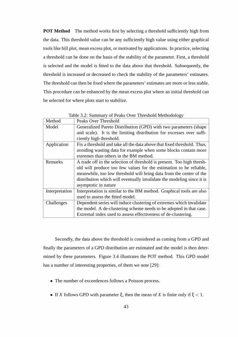
POT Method The method works first by selecting a threshold sufficiently high from

the data. This threshold value can be any sufficiently high value using either graphical

tools like hill plot, mean excess plot, or motivated by applications. In practice, selecting

a threshold can be done on the basis of the stability of the parameter. First, a threshold

is selected and the model is fitted to the data above that threshold. Subsequently, the

threshold is increased or decreased to check the stability of the parameters’ estimates.

The threshold can then be fixed where the parameters’ estimates are more or less stable.

This procedure can be enhanced by the mean excess plot where an initial threshold can

be selected for where plots start to stabilize.

Table 3.2: Summary of Peaks Over Threshold MethodologyMethod Peaks Over ThresholdModel Generalized Pareto Distribution (GPD) with two parameters(shape

and scale). It is the limiting distribution for excesses over suffi-ciently high threshold.

Application Fix a threshold and take all the data above that fixed threshold. Thus,avoiding wasting data for example when some blocks contain moreextremes than others in the BM method.

Remarks A trade off in the selection of threshold is present. Too highthresh-old will produce too few values for the estimation to be reliable,meanwhile, too low threshold will bring data from the centerof thedistribution which will eventually invalidate the modeling since it isasymptotic in nature

Interpretation Interpretation is similar to the BM method. Graphical tools are alsoused to assess the fitted model.

Challenges Dependent series will induce clustering of extremes which invalidatethe model. A de-clustering scheme needs to be adopted in thatcase.Extremal index used to assess effectiveness of de-clustering.

Secondly, the data above the threshold is considered as coming from a GPD and

finally the parameters of a GPD distribution are estimated and the model is then deter-

mined by these parameters. Figure 3.4 illustrates the POT method. This GPD model

has a number of interesting properties, of them we note [29]:

• The number of exceedences follows a Poisson process.

• If X follows GPD with parameterξ, then the mean ofX is finite only if ξ < 1.

43

• The empirical mean excess function can be used in the threshold selection, the

threshold will be from the region where mean excess plot starts to stabilize.

3.2.3 r-largest order statistics Model

The r-largest order statistics method is the third model to be discussed based on EVT.

r-largest order statistics method comes as an extension and improvement over the tradi-

tional block maxima method. It is a halfway between the BM and the POT. Inr-largest

order statistics, data are segmented into adjacent blocks and from each block ther

largest observations are selected and fitted into a joint GEVdistribution [99].

DefineMn,k to be thekth largest observation in(X1,X2, . . . ,Xn). If Equation 3.2

holds, then the distribution of the properly centralized and scaled sequence of largest

order maxima is

P[Mn,k−bn)/an ≤ x]→ Gk(x) (3.11)

on{x : 1+ξ(x−m)/σ} whereGk(x) = e−τ(x)∑k−1s=0

τ(x)ss! with τ(x) = [1+ξ(x−µ

σ )]− 1

ξ where

µ is the location parameter,σ is the scale parameter, andξ is the shape parameter [21].

The parameters to be estimated in this model are the triplet(ξ,µ,σ), where they

have the same interpretations as in the block maxima method.Assuming the indepen-

dence among the observations, the method of estimation usesthe same widely available

methods of maximum likelihood methodology.

The value ofr which represents the number of high order statistics to be selected

from each block is subject to some tradeoff between the variance and the accuracy as

in the block size selection in BM and the threshold selection in POT methods. A large

value forr will produce too many values that the asymptotic nature of the model will

be put in doubt. On the other hand a small value forr will produce wide confidence

intervals for the parameters’ estimates that the confidencein the model will be put in

doubt. A balance needs to be reached [21].

44

0 5 10 15 20 25 300

0.5

1

1.5

2

2.5

3

3.5

4

4.5

5x 10

4

Bitrate

The

mag

itude

threshold u=1.8

Figure 3.4: Peaks Over Threshold Method

Table 3.3: Summary ofr-largest order statistics MethodologyMethod r-largest order statistics (RLOS)Model Generalized Extreme Value Distribution as in the BM methodApplication Data are segmented into blocks and from each block ther largest

are picked and a new series is constituted that has ther largest fromeach block. To this new series the GEV is fitted

Remarks The selection ofr is crucial. Too smallr will produce model parame-ters with very large confidence intervals, which is not desirable sincethere will be no precision. Very large r order will eventually includeobservations from the center of the distribution which invalidate themodel assumption altogether.

Interpretation It is similar to the BM method. Few values of r can be tested andfrom the graphical tools the model can be assessed. Increasing thevalue of r improve the quality of estimates, but not to increase veryfar.

Challenges Selecting the right number of order statistics to be included in themodel fitting.

Some studies that have applied this model in hydrology suggested value ofr in

the range 3-7 [27]. However, this is not necessarily the casein the traffic data and we

can only tell after carefully studying traffic data model estimates.

45

3.2.4 Return Level and Return Period

Return level and return period are two prediction methods forapplying Extreme Value

Theory [43, 29]. Return level is the value that is expected to occur once during a return

period. It answers questions like what is the mean waiting time between very large

events that exceeds the return level. So, T-year return level is the value that will be

exceeded on average once in a T-year time, year can be replaced by the appropriate

blocking structure. For example, if data are blocked according to minutes, then only

would it make sense to talk about T-minutes. In Finance literature the same concept is

applied and it is referred to as Value at Risk (VaR) [91].

The return period gives the mean expected time between two specific extreme

events. To calculate them we need first to estimate the quantiles of the block maximum

distribution. This is achieved by inverting Equation (3.6).

xp = µ−σξ

[

1−{−log(1− p)}−ξ]

, ξ 6= 0, (3.12)

and in the case the parameterξ is equal to zero, the above equation becomes

xp = µ−σ log{− log(1− p)} , ξ = 0 (3.13)

whereG(xp) = 1− p and 0< p< 1, [29]. To a reasonable degree of estimation, 1/p

is the return period andxp is the associated return level. This prediction tool produces

some measures of extremes in the network. These measures canthen be incorporated

into future service level agreements.

However, to use this tool it is necessary to estimate the corresponding GEV pa-

rameters and plug them back into Equations 3.12 and 3.13. Figure 3.5 illustrates a

return level plot for some of the external traffic traces which was first fitted into a GPD

with a threshold 4000 bytes. The plot can be interpreted in particular context. In this

example, the plot is being produced for the bit rate of the external traffic data. The data

are fitted to a GPD with a threshold of 4 kilo byte. The horizontal axis shows the bit

46

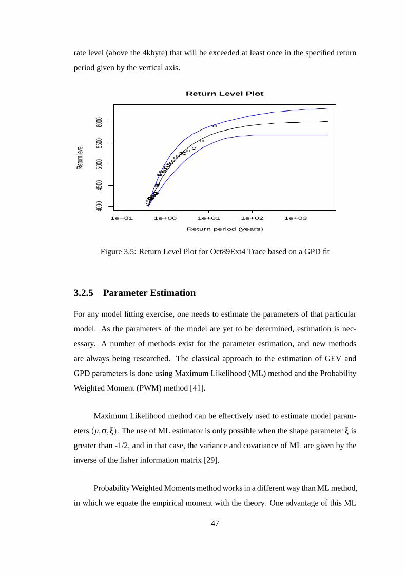
rate level (above the 4kbyte) that will be exceeded at least once in the specified return

period given by the vertical axis.

1e−01 1e+00 1e+01 1e+02 1e+03

4000

4500

5000

5500

6000

Return Level Plot

Return period (years)

Retur

n leve

l

Figure 3.5: Return Level Plot for Oct89Ext4 Trace based on a GPD fit

3.2.5 Parameter Estimation

For any model fitting exercise, one needs to estimate the parameters of that particular

model. As the parameters of the model are yet to be determined, estimation is nec-

essary. A number of methods exist for the parameter estimation, and new methods

are always being researched. The classical approach to the estimation of GEV and

GPD parameters is done using Maximum Likelihood (ML) methodand the Probability

Weighted Moment (PWM) method [41].

Maximum Likelihood method can be effectively used to estimate model param-

eters(µ,σ,ξ). The use of ML estimator is only possible when the shape parameterξ is

greater than -1/2, and in that case, the variance and covariance of ML are given by the

inverse of the fisher information matrix [29].

Probability Weighted Moments method works in a different way than ML method,

in which we equate the empirical moment with the theory. One advantage of this ML

47

method is that calculations are simple and regularity conditions are met whereξ in

[-1/2,1/2], [29]. However, PWM suffers from the fact that it has no guarantee of fea-

sibility and might yield non-feasible parameter estimates. The non-feasibility problem

decreases when some further conditions are satisfied [8].

Nevertheless, the recommended method for parameter estimation is the one based

on ML. It is widely used, and implemented in the popular data analysis software such

as R and MATLAB. Other approaches do exist for the estimation of GEV and GPD

parameters such as Bayesian and Robust approaches [50].

Maximum Likelihood Estimation

The ML method is a popular method for estimating many model parameters. It is

widely used, acceptable, and possesses good properties. Itworks first by constructing

a likelihood function, and then maximizes the likelihood function with respect to the

desired parameters.

Definition For each sample pointx, let θ(x) be a parameter value at which the like-

lihood functionL(θ|x) attains its maximum as a function ofθ, with x held fixed. A

maximum likelihood (ML) of the parameterθ based on a sampleX is θ(X).

Suppose we haveX1,X2, . . . ,Xn are i.i.d. samples from a population that has a

probability distribution function given byf (x|θ1,θ2, . . . ,θk), the likelihood function is

given by [29]

L(θ|X) = L(θ1,θ2, . . . ,θk|x1,x2, . . . ,xn) = ∏ i = 1n f (xi |θ1,θ2, . . . ,θk) (3.14)

The Maximum Likelihood Estimator (MLE) is given as the valueof θ at which the

ML function attains its maximum. To find this value, we assumethat the ML function

is differentiable and we differentiate it and equate it to zero to find the maximum value

48

of the function and henceθ

∂∂θi

L(θ|X)∣

∣

∣θ = 0, i = 1,2, . . . ,k,θ ∈ Θ ⊂ Rk (3.15)

In general and in all ML estimations, ML procedures suffer from two things,

finding a global maximum of the likelihood function and verifying indeed that it is a

global maximum not a local one. And the second issue is whether MLE is numerically

sensitive. This second point is a mathematically inheritedproblem [86].

The confidence intervals for the estimator, which depend on the Fisher informa-

tion matrix, are calculated either by analytically drivingthe fisher information matrix

or by making use of the observed information matrix. In practice we use the inverse of

the observed information matrix [86].

GEV ML Estimation The log likelihood function for a sampleY1, . . . ,Ym of i.i.d.

GEV model is given by [8]

logL(ξ,µ,σ) =−mlogσ− (1ξ+1)

m

∑i=1

log(1+ξYi −µ

σ)−

m

∑i=1

(1+ξYi −µ

σ)− 1

ξ (3.16)

In the caseξ = 0, the above will not work (divide by zero!), and we have another log

likelihood for that case

logL(0,µ,σ) =−mlogσ−m

∑i=1

exp(−Yi −µ

σ)−

m

∑i=1

Yi −µσ

(3.17)

GEV likelihood functions have no analytical solution to determine the(ξ,µ,σ), they

need to be numerically evaluated. If the iterated value is inthe regionξ>−1 we can get

a local maximum. The good estimators properties such as being asymptotically efficient

and normal do still hold. However, a local maximum cannot be obtained in case the

shape parameter value is in the regionξ <−1, this problem is discussed thoroughly by

Smith in [88].

49

GPD ML estimation Having an i.i.d. sampleY1,Y2, . . . ,Yn drawn from a GPD with

parameters(ξ,β), the likelihood function is given by [8]

l((ξ,β),Y1, . . . ,Yn) =−nlnβ− (1ξ+1)

n

∑i=1

ln(1+ξβ

Xi) (3.18)

This likelihood function needs to be dealt with numericallyas it is the case in the

GEV maximum likelihood estimation. The function works and have local maxima for

the caseξ >−1/2, the asymptotic normality is obtained and given by [29]

n1/2(ξn−ξ,βn

β−1)→ N(0,M−1),n→ ∞ (3.19)

with M−1 = (1+ξ)

1+ξ 1

1 2

.

Method of Moment Estimator (MME)

The essence of method of moment estimates is in equating the sample moment with

the population moment. We obtain then a system of equations that we solve to get the

parameter estimates [87].

The MME is obtained by solving the system

E(Xr) =1n

n

∑i=1

Xri , r = 1, . . .k (3.20)

wherek is the dimension of parameter spaceΘ, andθ = {θ1,θ2, . . .θk}. Sometimes

MME produces unreliable results. However, it is used as an initial estimator in numer-

ical calculations. Also, the MLEs of GEV is such a case where we may use MME as

initial estimator to supply to our numerical algorithm.

An improvement of the MME is given by the introducing some weights to the

calculations. The idea is to use empirical weights based on the CDF and equate them

with their theoretical counterparts in the other side of equation [8]. Such a method is

called Method of Probability Weighted Moment (PWM). Obviously, the advantage of

50

PWM is due to the more efficient use of the available data. Theoretically, the weighted

moment is given as

E(Xr [F(X;θ)]s[1−F(X;θ)]t) (3.21)

and their empirical counterparts are given as

1n

n

∑i=1

xri:nps

i:n(1− pi:n)t (3.22)

wherer = 1, . . . ,k;xi:n is theith order sample statistics andpi:n is theith plotting posi-

tion. Having these two equations, then we equate them and solve the resulting system

of equations to get the PWM estimates. In case of GEV model, it is easy to show that

E(X(F(X))r) can be written as [29]

βr =1

r +1

{

µ−σξ

[

1− (r +1)ξΓ(1−ξ)]

}

, ξ < 1 (3.23)

whereΓ stands for the Gamma function,Γ(t) =∫ ∞

0 e−uut−1du, t > 0 The estimators

(ξ, µ, σ) are simply the solution of the system :

β0 = µ− σξ (1−Γ(1−ξ))

2β1−β0 =σξ Γ(1−ξ)(2ξ −1)

3β2−β02β1−β0

= 3ξ−12ξ−1

(3.24)

and replacingβr by its unbiased estimator gives

βr =1n

n

∑j=1

(

r

∏l=1

j − ln− l

)

Xj,n (3.25)

with the usual convention where(X1,n, . . . ,Xn,n) is the ordered GEV sample.

3.3 Model Diagnostics

Selecting the right model is as important as the modeling itself. A great deal of work

has been done to illustrate this point [93]. It is thus important to let the data speak

for itself; this can be done by visualizing the data using different graphical tools. The

51

collection of these graphical techniques is given the name Exploratory Data Analysis

(EDA). Selecting the right model will make burst predictionmore accurate. In turn,

accurate prediction of traffic bursts leads naturally to an enhanced Quality of Service.

In this section, we will discuss some of EVT based model selection tools. Namely,

Records, Maximum to Sum Ratio, Gumbel Plot, Hill Plot, QQ Plot,quantile plot, and

Mean Excess plot. We illustrate some of these tools with examples.

3.3.1 Records

Records can be used as exploratory tool in distinguishing between independent identi-

cally distributed data (i.i.d.) and non i.i.d. data. Recordsmake use of a known pattern

of records from (i.i.d.). In fact, the number of records fromi.i.d. data grows very slowly

[29]. This fact allows us to use the number of recordsN in our traffic data and compare

with expected records in a typical known i.i.d. data. If there is a match in the number

of records, then we may say that our traffic data can be modeledas i.i.d. otherwise we

say that our data cannot be modeled as coming from i.i.d. random process.

A recordXn occurs if

Xn > Mn−1 = max(X1, . . . ,Xn−1) (3.26)

By definitionX1 is a record. LetI be an indicator function, the record counting process

N is given as

N1 = 1, Nn = 1+n

∑k=2

IXk>Mk−1, n≥ 2. (3.27)

The expected value of the number of records counting processin i.i.d. settings is given

by E(Nn) = ∑nk=1

1k , and the variance of that process is given byVar(Nn) = ∑n

k=1(1k −

1k2). It increases with the increasing of the sample size. For example in 100 i.i.d. we

expect 5 records,E(N100) = 5.2, when the size of the sample increases to 1000, then

the expected number of records increases to 7, we haveE(N1000) = 7.

52

3.3.2 Maximum to Sum Ratio

Maximum to sum ratioMn/Sn can be used as an explanatory tool to tell about the finite-

ness (existence) of the moment of given order, sayp [71]. It is a standard knowledge

that the mean and variance of a given data are their first ordermoment and second order

moment, respectively.

Using maximum to sum ratio, we are able to tell whether the variance, which is

the second order moment, of data is finite (exists) or infinite(does not exist). Thepth

order partial sum andpth order maximum are given by

Sn(p) = ∑ni=1 |X|p andMn(p) = max(|X1|

p, . . . , |Xn|p), respectively [29].

From [29], we have the following equivalence relation

Rn(p) = Mn(p)/Sn(p)→ 0⇔ E|X|p < ∞ (3.28)

This equivalence relation means thatpth order maximum topth order partial sum

ratio goes to 0 asn approaches infinity if and only if thepth order moment exists.

A direct way to use the above fact is to plot the max to sum ratiofor different order

moments. If the plot for a given moment order goes to zero, then we conclude that the

moment of that order is finite (exists). It is to note that a heavy tail distribution with tail

parameterα < 2 has an infinite variance and ifα < 1, the mean is also infinite.

To illustrate this tool, we know that if the moment of the firstorder which is the

mean does not exists then neither the mean is finite nor does the variance exist too. We

tested a sample of 100 realizations from a Pareto distribution with parameterα = 1.5.

In this setting, it is obvious that the mean does exist and is finite but not the variance

which is infinite.

We plotted both the maximum to sum ratio for the first order andsecond order

moments usingp= 1 andp= 2, respectively. Since the mean is finite, the maximum

to sum ratio withp = 1 will produce a plot that will converge to zero as the number

of realizations increases. However, the variance is infinite, this means of we plot the

53

maximum to sum ratio withp= 2, the plot will not converge to zero and will continue

to fluctuate. This is illustrated by the Figure 3.6.

0 2000 4000 6000 8000 100000

0.2

0.4

0.6

0.8

1

(a) Pareto random vairable sample with alpha=1.5

Max

/Sum

Rat

io, p

=1

0 2000 4000 6000 8000 100000

0.2

0.4

0.6

0.8

1

(b) Pareto random vairable sample with alpha=1.5

Max

/Sum

Rat

io, p

=2

Figure 3.6: Max/sum ratio with p=1 and p=2 for top and bottom,respectively

Figure 3.6 (a) shows the Maximum to Sum ratio forp= 1. Since plots are con-

verging to zero, it shows that the mean is finite which is the first order moment. How-

ever, for the second order moment (p = 2) shown in Figure 3.6 (b), it is evident that

the plots do not converge. Hence, it is concluded that for this data the second order

moment does not exist.

Maximum to sum ratio is used for other purposes as well. It used for estimation

purposes. Max to sum ratio is suggested as a test statistics in estimating the tail index

of a very heavy tail distributions [67]. In particular, whenthe tail indexα approaches

zero, which is the case of a super heavy tail probabilities.

54

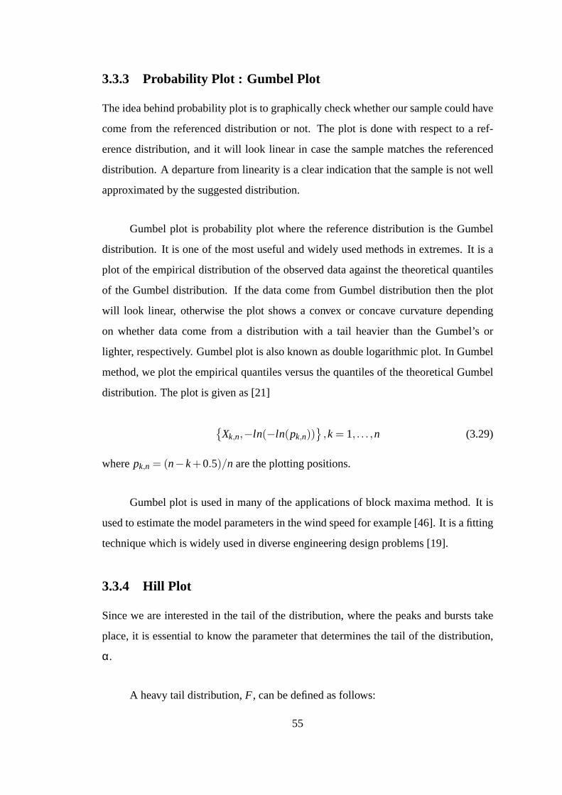
3.3.3 Probability Plot : Gumbel Plot

The idea behind probability plot is to graphically check whether our sample could have

come from the referenced distribution or not. The plot is done with respect to a ref-

erence distribution, and it will look linear in case the sample matches the referenced

distribution. A departure from linearity is a clear indication that the sample is not well

approximated by the suggested distribution.

Gumbel plot is probability plot where the reference distribution is the Gumbel

distribution. It is one of the most useful and widely used methods in extremes. It is a

plot of the empirical distribution of the observed data against the theoretical quantiles

of the Gumbel distribution. If the data come from Gumbel distribution then the plot

will look linear, otherwise the plot shows a convex or concave curvature depending

on whether data come from a distribution with a tail heavier than the Gumbel’s or

lighter, respectively. Gumbel plot is also known as double logarithmic plot. In Gumbel

method, we plot the empirical quantiles versus the quantiles of the theoretical Gumbel

distribution. The plot is given as [21]

{

Xk,n,−ln(−ln(pk,n))}

,k= 1, . . . ,n (3.29)

wherepk,n = (n−k+0.5)/n are the plotting positions.

Gumbel plot is used in many of the applications of block maxima method. It is

used to estimate the model parameters in the wind speed for example [46]. It is a fitting

technique which is widely used in diverse engineering design problems [19].

3.3.4 Hill Plot

Since we are interested in the tail of the distribution, where the peaks and bursts take

place, it is essential to know the parameter that determinesthe tail of the distribution,

α.

A heavy tail distribution,F , can be defined as follows:

55

Definition [80] Suppose we have a sampleX1,X2, . . . ,Xn that follows a distribution

F(x), we sayF(x) is heavy tailed with indexα if P(X > x) = F(x) = x−αL(x), x> 0

whereL(x) is a slowly varying function.

To characterize and define exactly the heavy tail distribution, we need to specify

exactly or to a reasonable degree the value of the parameterα. Hill estimator is a

popular method for estimating the parameterα, eventually some difficulties exist with

this method. Hill estimator is defined as follows [29]

Hk,n =1k

k

∑i=1

logX(i)

X(k+1)(3.30)

whereX(i) is the ith largest value in the sample. To make full use of Hillestimator, we

plot (k,H−1k,n ), 1≤ k≤ n. We pick the parameterα from the region where the graph is

becoming stable. As an example we simulate 100 Pareto samplewith α = 1.2 and we

plot the Hill plot and try to see if we can deduce the value of alpha from the graph.

Figure 3.7 shows two Hill plots for internal traffic and external traffic. Plot (a)

shows WAN traffic. Its corresponding Hill plot is shown in plot (c). In the second

column in plot (b) is shown the LAN traffic data of bit rate and in the plot (d) the

corresponding Hill plot is shown. Both Hill plots are being produced with 95 percent

confidence intervals, shown by the jagged line.

Hill plot is used primarly in estimating the heavy tail indexalpha. Its use and

even introduction started with applications in hydrology [29]. However, with the dis-

covery of many natural events that are heavy tailed, its use has become a standard

practice in the estimation.

3.3.5 Quantile-Quantile Plot

Quantile-Quantile Plot (QQ-Plot) is an effective tool usedin comparing samples from

possibly different distributions [80]. In QQ-Plot, we plotthe quantile of a two dif-

ferent distributions. QQ-plot is used in statistical inference by plotting quantiles from

unknown distribution against quantiles from a hypothetical distribution with known

56

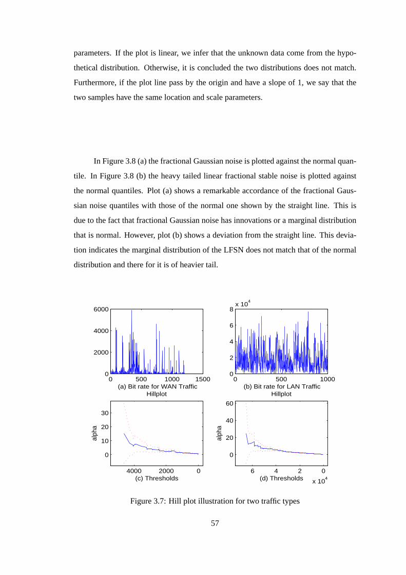
parameters. If the plot is linear, we infer that the unknown data come from the hypo-

thetical distribution. Otherwise, it is concluded the two distributions does not match.

Furthermore, if the plot line pass by the origin and have a slope of 1, we say that the

two samples have the same location and scale parameters.

In Figure 3.8 (a) the fractional Gaussian noise is plotted against the normal quan-

tile. In Figure 3.8 (b) the heavy tailed linear fractional stable noise is plotted against

the normal quantiles. Plot (a) shows a remarkable accordance of the fractional Gaus-

sian noise quantiles with those of the normal one shown by thestraight line. This is

due to the fact that fractional Gaussian noise has innovations or a marginal distribution

that is normal. However, plot (b) shows a deviation from the straight line. This devia-

tion indicates the marginal distribution of the LFSN does not match that of the normal

distribution and there for it is of heavier tail.

0 500 1000 15000

2000

4000

6000

(a) Bit rate for WAN Traffic

020004000

0

10

20

30

(c) Thresholds

alph

a

Hillplot

0 500 10000

2

4

6

8x 10

4

(b) Bit rate for LAN Traffic

0246

x 104

0

20

40

60

(d) Thresholds

alph

a

Hillplot

Figure 3.7: Hill plot illustration for two traffic types

57

−4 −2 0 2 4−1.5

−1

−0.5

0

0.5

1

1.5

(a) QQ−Plot of Internal Traffic Data

Qua

ntile

s of

Sim

ulat

ed In

tern

al T

raffi

c (F

GN

)

QQ Plot of Sample Data versus Standard Normal

−4 −2 0 2 4−10

0

10

20

30

40

50

60

70

80

(b) QQ−Plot of External Traffic Data

Qua

ntile

s of

Sim

ulat

ed E

xter

nal T

raffi

c (L

FSN

)

QQ Plot of Sample Data versus Standard Normal

Figure 3.8: QQ-Plot Illustration

3.3.6 Quantile Plot

Quantile plot is totally different from Quantile-Quantileplot. Quantile plot, sometimes

referred to as Qplot, is a plot that examines a single variable data set. Quantile-Quantile

plot is for the comparison of two samples from possibly different distributions. In

Quantile plot we plot the data against standard quantile that is comparing one sample

of the data to the standard quantiles or to itself. While in theother method, Quantile-

Quantile plot, we take two sample or datasets and we compare their quantiles by plot-

ting their quantiles against each other. This second methodis used to compare two

samples and see if they have the same parent theoretical distribution or not.

Quantile plot can help in obtaining valuable information about the data like me-

dian, quantiles and interquantile range. Such informationcan be easily obtained from

simple look at the Quantile plot. The slope of the quantile plot will indicate the density

of the data. The flatter the slope is the denser are the data at that area.

Suppose we have a sample ofn data pointsy1,y2, . . . ,yn for which we would like to ob-

58

tain its quantile plot. To plot, we arrange the data in ascending ordery(1),y(2), . . . ,y(n)

with y(1) being the smallest and letpi = i/n, i = 1, . . . ,n be a fraction in [0,1]. Define

the quantileQ(pi) to bey(i). The plot{pi ,Q(pi)} is called the quantile plot.

3.3.7 Mean Excess Plot

The mean excess function of a probability distribution is given ase(u) = E(X−u|X >

u), 0≤ u< xF , whereu is a given threshold andxF is the support or right end point

of the distribution [29].

Mean excess function is used under different names in different disciplines. In

insurance, it is the expected claim size in the unlimited layer; in finance, it is the short-

fall; in reliability, it is the mean residual life. Mean excess plot (meplot) is based on

the mean excess function. It is a useful visualization tool.Its importance comes from

the fact that it helps in discriminating in the tail of trafficdata. If traffic data comes

from a distribution with a heavier tail than Gumbel’s, then the plot will look linearly

increasing. If data come from a distribution with a lighter tail than the Gumbel, then

the mean excess plot will be linearly decreasing.

As a graphical tool we use the mean excess plot, it is based on the estimate of mean

excess function. Suppose that we haveX1,X2, . . . ,Xn, the sample mean excess is given

as

en(u) = 1/F(u)∫ ∞

uFn(y)dy (3.31)

The graph{Xk,n,en(Xk,n)} is called the mean excess plot.

As is apparent from both plots in Figure 3.9, the plots have different character-

istics. The internal traffic, plot (a) has a decreasing or negative slop as the threshold

increases. This plot was based on the authentic trace from Belcore about the internal

traffic. However, the external traffic in plot (b), which is based on simulated linear frac-

tional stable noise, shows an positive slope and it increases as the threshold increases.

This can be explained since the external traffic marginal distribution is heavy tailed, the

values tends to get larger and larger and eventually the meanis taken on few very large

values only as the threshold increases.

59

0 10 20 30 400

5

10

15

20

25

(b) Thrshold of simulated WAN Traffic based on lfsnM

ean

Exc

ess

0 2 4 6 8

x 104

0.4

0.6

0.8

1

1.2

1.4

1.6

1.8x 10

4

(a) Thrshold of LAN Traffic

Mea

n E

xces

s

Figure 3.9: Mean Excess Plot for Internal and External Traffic

3.4 Extremal Index

Much of the above theory have been discussed in a setting thatassumes stationarity and

independence of the data (i.i.d.). The reality is that real world problems are rarely in

such conformity to the i.i.d. case. More specifically, Internet and network traffic data

is very far from being independent or stationary. Fortunately, a recent upgrade to the

theory is being done by introducing the extremal index concept [57]. The extremal in-

dex allows for a successful implementation of the theory in the presence of a dependent

sequence. Thus it relaxes the independence assumption in the theory.

However, the type of distribution remains unchanged and theparameters will vary

slightly in the later of dependence. However, it should not be a problem since they have

to be estimated in either case.

The two conditions to be satisfied are called Leadbetter’s mixing conditions D and

D’ which deal with long range and local mixing [57]. If the twoconditions are satisfied,

the GEV theory and the GPD will still be applied with the introduction of the extremal

index parameter calledθ which range between zero and one. Zero being for strongly

dependent and one for the independent case. The extremal index can be thought of as

60

the reciprocal of mean cluster size [21] givn as

P{max(X1,X2, . . . ,Xn)≤ x} ≈ Fθn(x) (3.32)

There are a number of approaches to estimate the extremal index θ , basically three

approaches. The block method, the run method, and the inter-exceedance times method

and some variants of these three methods, see [83]. The blockmethod works by seg-

menting the data into consecutive blocks of equal lengths. The number of exceedances

over some high threshold are counted from each block, the estimator is taken then to

be the reciprocal of the average exceedances per block. We chose this method which is

relatively easy and yet reliable.

3.5 Simulation

The study of the bursts in the traffic could not be complete without addressing simu-

lation techniques given their significance in computer networks. As modeling is about

representing data in abstract terms, simulation is about generating data out of that ab-

stract model. The need for simulation in computer networks is of great importance not

only to gauge the abstract model, but for other uses like performance evaluations and

network planning. In some situations like when a network to be built is still in the plan-

ning process, the only way to test that network and avoid future large scale deficiencies

is through the simulation process.

Simulation can be explained into two categories depending on events type, dis-

crete event simulation and continuous event simulation [7]. Both discrete and contin-

uous refers to the time at which events happen, as the name suggests, the continuous

events simulation is suitable for events that take place in continuous time like mea-

suring temperature for example, while discrete events is the one suitable for computer

networks where the events, be it packets arrival at the edge of the router for examples,

happen in a discrete manner.

61

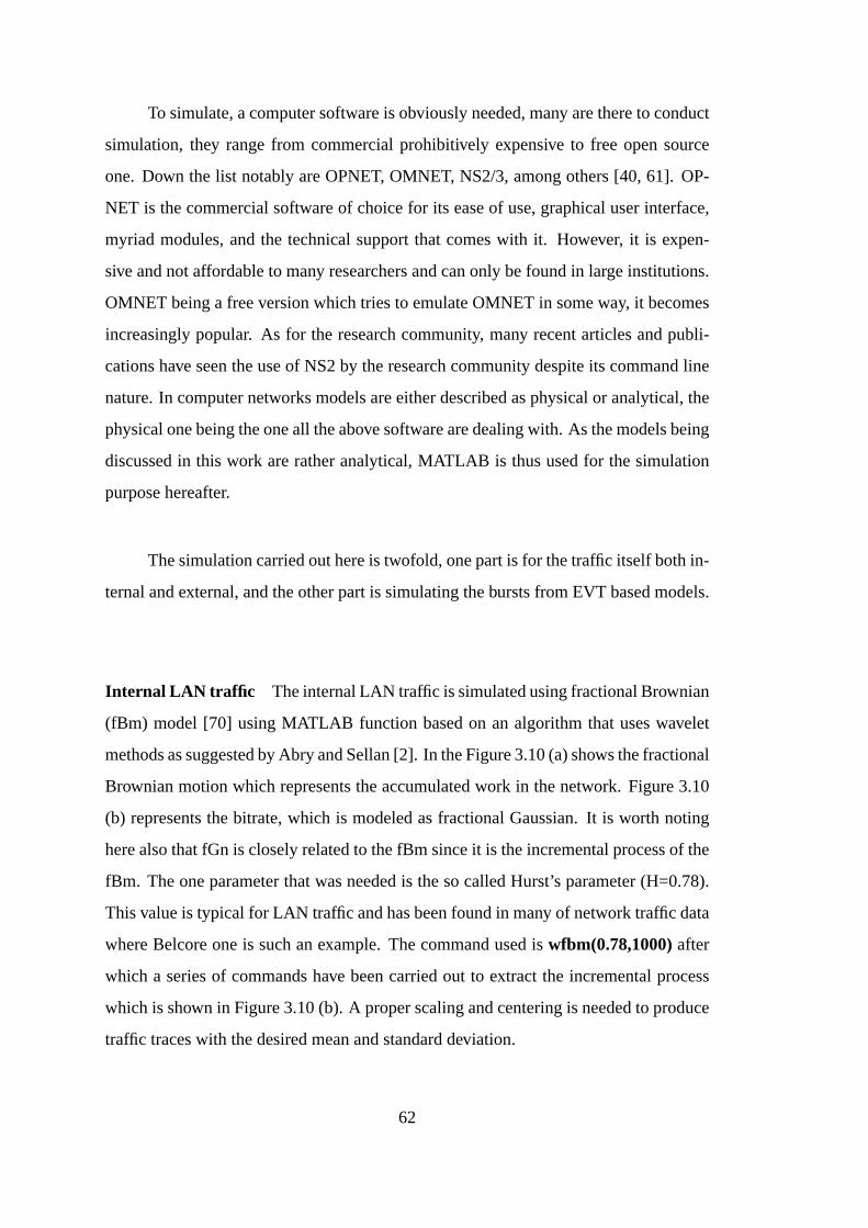
To simulate, a computer software is obviously needed, many are there to conduct

simulation, they range from commercial prohibitively expensive to free open source

one. Down the list notably are OPNET, OMNET, NS2/3, among others [40, 61]. OP-

NET is the commercial software of choice for its ease of use, graphical user interface,

myriad modules, and the technical support that comes with it. However, it is expen-

sive and not affordable to many researchers and can only be found in large institutions.

OMNET being a free version which tries to emulate OMNET in some way, it becomes

increasingly popular. As for the research community, many recent articles and publi-

cations have seen the use of NS2 by the research community despite its command line

nature. In computer networks models are either described asphysical or analytical, the

physical one being the one all the above software are dealingwith. As the models being

discussed in this work are rather analytical, MATLAB is thusused for the simulation

purpose hereafter.

The simulation carried out here is twofold, one part is for the traffic itself both in-

ternal and external, and the other part is simulating the bursts from EVT based models.

Internal LAN traffic The internal LAN traffic is simulated using fractional Brownian

(fBm) model [70] using MATLAB function based on an algorithm that uses wavelet

methods as suggested by Abry and Sellan [2]. In the Figure 3.10 (a) shows the fractional

Brownian motion which represents the accumulated work in thenetwork. Figure 3.10

(b) represents the bitrate, which is modeled as fractional Gaussian. It is worth noting

here also that fGn is closely related to the fBm since it is the incremental process of the

fBm. The one parameter that was needed is the so called Hurst’sparameter (H=0.78).

This value is typical for LAN traffic and has been found in manyof network traffic data

where Belcore one is such an example. The command used iswfbm(0.78,1000)after

which a series of commands have been carried out to extract the incremental process

which is shown in Figure 3.10 (b). A proper scaling and centering is needed to produce

traffic traces with the desired mean and standard deviation.

62

0 1000 2000 3000 4000 5000−50

0

50

100

(a) Fractional brownian motion, simulating accumlated work

Accu

mu

late

d b

itra

te

0 1000 2000 3000 4000 5000−1

−0.5

0

0.5

1

(b) The increment process of fBm, simulating the bitrate

Bitra

te

Figure 3.10: Simulating Internal LAN traffic using fBm

External WAN traffic The external WAN traffic simulation is also carried out using

MATLAB. External WAN traffic demonstrate properties that aredifferent from internal

traffic and thus the model suggested for the external WAN traffic is the Linear Fractional

Stable Motion (LFSM) as suggested in the literature by Stilian and Taqqu, see [2] and

the references therein. LFSM is also a self-similar processand the fractional Gaussian

noise is just a special case of it. While the increments in the fBm are normally dis-

tributed, the difference is that in the case of LFSM the increments are distributed with a

Pareto type heavy tail distribution, the parameter that controls the degree of heavy tail

is called alpha.

63

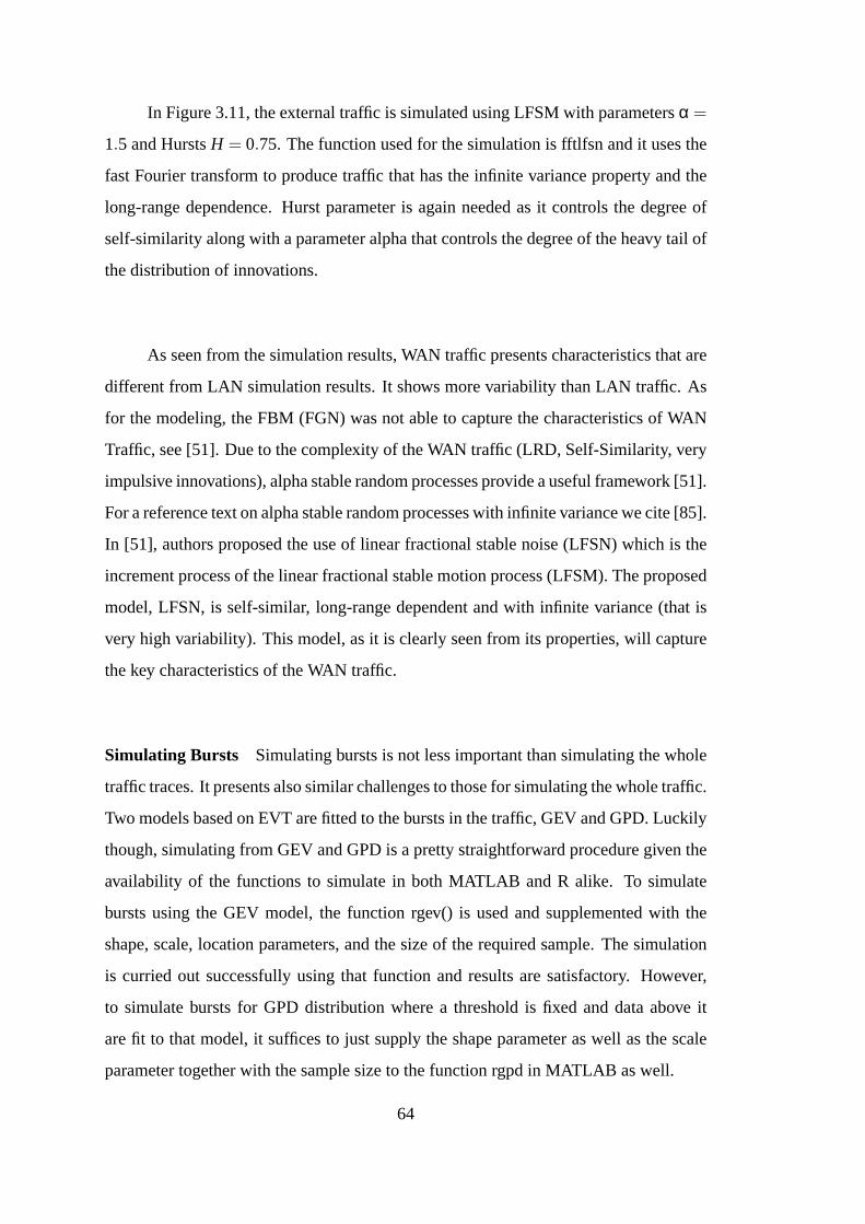
In Figure 3.11, the external traffic is simulated using LFSM with parametersα =

1.5 and HurstsH = 0.75. The function used for the simulation is fftlfsn and it uses the

fast Fourier transform to produce traffic that has the infinite variance property and the

long-range dependence. Hurst parameter is again needed as it controls the degree of

self-similarity along with a parameter alpha that controlsthe degree of the heavy tail of

the distribution of innovations.

As seen from the simulation results, WAN traffic presents characteristics that are

different from LAN simulation results. It shows more variability than LAN traffic. As

for the modeling, the FBM (FGN) was not able to capture the characteristics of WAN

Traffic, see [51]. Due to the complexity of the WAN traffic (LRD,Self-Similarity, very

impulsive innovations), alpha stable random processes provide a useful framework [51].

For a reference text on alpha stable random processes with infinite variance we cite [85].

In [51], authors proposed the use of linear fractional stable noise (LFSN) which is the

increment process of the linear fractional stable motion process (LFSM). The proposed

model, LFSN, is self-similar, long-range dependent and with infinite variance (that is

very high variability). This model, as it is clearly seen from its properties, will capture

the key characteristics of the WAN traffic.

Simulating Bursts Simulating bursts is not less important than simulating thewhole

traffic traces. It presents also similar challenges to thosefor simulating the whole traffic.

Two models based on EVT are fitted to the bursts in the traffic, GEV and GPD. Luckily

though, simulating from GEV and GPD is a pretty straightforward procedure given the

availability of the functions to simulate in both MATLAB andR alike. To simulate

bursts using the GEV model, the function rgev() is used and supplemented with the

shape, scale, location parameters, and the size of the required sample. The simulation

is curried out successfully using that function and resultsare satisfactory. However,

to simulate bursts for GPD distribution where a threshold isfixed and data above it

are fit to that model, it suffices to just supply the shape parameter as well as the scale

parameter together with the sample size to the function rgpdin MATLAB as well.

64

0 500 1000 1500 2000 2500 3000 3500 4000 4500 50000

5

10

15

20

25

Figure 3.11: Simulating External WAN Traffic using LFSM

3.6 Summary

In this chapter, we presented the theory behind our methodology with a brief account

to the development of Extreme Value Theory. We presented also the estimation proce-

dures for the proposed models. An extensive list of the modelselection and validation

tools is also presented. These tools are to be used selectively and the choice is left to

the practitioner to decide on which one to include in the analysis.

65

CHAPTER 4

EXPERIMENTAL RESULTS AND ANALYSIS

In this section, the analysis starts by describing trace data. Then it proceeds by applying

some exploratory data analysis to the selected datasets foran informed guess of the

behavior of the dataset in hand. Applications of GEV, GPD, and RLOS models based

on EVT are shown. Evaluation using some diagnostics graphical checks of the models

is then presented followed by discussion and summary.

4.1 Exploratory Analysis

A lot of effort can be saved by first visualizing the availabledata. Doing so, useful

information can be extracted from the graphs. For example, one can tell whether a

trend is present in the data, whether data are stationary. Further question such as, are

they independent or strongly correlated?, can be readily answered. However, it is not

easy for the first time to tell all these information by merelylooking into these graphs.

It requires an adequate practice and training to be able to spot all these details from

a simple glance. Fortunately, in this era of available computer power, high quality

graphs can be produced easier and the learning curve from these graphs is becoming

less steep as well. Checking the data and plotting some graphsto visualize data is an

important step toward a successful modeling exercise. Suchstep is called exploratory

data analysis and it plays a great deal in deciding on the right model to be fitted to data.

Whether data can be approximated as stationary or blatantly non-stationary can also be

depicted from the graphical assessment.

It pays back to check the stationarity of the data at the first place. Stationarity

means that the law governing the process is not changing withtime, a property that is

crucial for the analysis and prediction to be relevant [45].If the mean or variance of

the data changes with time, then the prediction based on stationary model is doomed

to failure. In simpler words, the mean and variance should not change significantly

between the beginning of the data, the middle, and the end of the data if a stationary

model is to be used [45]. Exploratory data is used to check thestationarity of the

data by looking at the figure and check weather trends are present. However, more

robust stationarity checks are also possible [10]. For the purpose of EVT analysis, the

stationarity assumption found here is fairly acceptable.

The data being examined are high resolution internal and external network traf-

fic traces. They were collected at Belcore laboratories usingspecialized equipments.

These data were the subject of the seminal study discoveringthe self-similar and frac-

tal properties in network traffic by Leland et al [58]. Numerous researchers followed

through and used the data for other research purposes as well. Our objective from using

the same data is to predict bursts and serious deteriorations in the network bytes count

time series. The datasets are summarized in Table 4.1.

Table 4.1: Summary of Belcore WAN & LAN Packet TracesDataset Date Duration What SizeBC-pAug89 August 29, 1989 3142.82 Seconds Internal LAN 1,000,000BC-pOct89 October 5, 1989 1759.62 Seconds Internal LAN 1,000,000BC-Oct89Ext October 3, 1989 122797.83 External WAN 1,000,000BC-Oct89Ext4 October 10, 1989 215 Hours External WAN 1,000,000

The four datasets are the mixture of internal and external traces from Belcore

traces. Two traces (BC-pAug89, BC-pOct89) are internal LAN traces and the other

two (BC-Oct89Ext, BC-Oct89Ext4) are External WAN traces. Two simulated traces

for both internal and external traffic based on fractional Gaussian noise (fGn) and linear

fractional stable noise (LFSN), respectively, are also used to check the properties of the

fitted model [2, 89]. The original Belcore traces are composedof one million events

each, arranged in columns format, one column records the arrival time of the packet

and the other for the size of the arriving packet along with other state information. For

the purpose of this study and since the objective is to study traffic bursts, spikes, and

68

serious deteriorations, the data rate per time interval (100 millisecond=0.1 second), or

bytes counts / 0.1 second is used. Data is then transformed into bytes per 0.1 second

in MATLAB with some simple routines. It follows that bytes count per 0.1 second is

obtained.

After successfully transforming the traces into the desired state, simple plots of

both data are produced. They are shown in Figure 4.1. In that Figure, plot (a) shows the

internal LAN trace while plot (b) shows the external WAN traffic. Both plots are in the

0.1 second scale for the time, and bytes for the data. Traffic traces look bursty, which is

obvious in both internal and external traffic, especially inthe latter. This same behavior

persists when the aggregated data is plotted in the same fashion which is an indication

of the scale invariance property discussed earlier in Chapter 2. This is exactly what is

expected given the self-similar property of the traffic. However, the interest here lies

solely on the spikes and bursts in traffic traces.

0 1000 2000 3000 4000 5000 6000 7000 8000 90000

5

10x 10

4

(a) pOct89 LAN Trace in 0.1 Seconds

Byte

s co

un

t

0 1000 2000 3000 4000 5000 6000 7000 8000 90000

2000

4000

(b) Oct89Ext4 WAN Trace in 0.1 Seconds

Byte

s co

un

t

Figure 4.1: (a) Internal LAN traffic, (b) External WAN Traffic

69

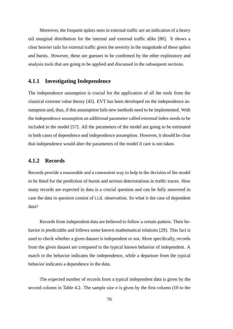
Moreover, the frequent spikes seen in external traffic are anindication of a heavy

tail marginal distribution for the internal and external traffic alike [80]. It shows a

clear heavier tails for external traffic given the severity in the magnitude of these spikes

and bursts. However, these are guesses to be confirmed by the other exploratory and

analysis tools that are going to be applied and discussed in the subsequent sections.

4.1.1 Investigating Independence

The independence assumption is crucial for the applicationof all the tools from the

classical extreme value theory [45]. EVT has been developedon the independence as-

sumption and, thus, if this assumption fails new methods need to be implemented. With

the independence assumption an additional parameter called extremal index needs to be

included in the model [57]. All the parameters of the model are going to be estimated

in both cases of dependence and independence assumption. However, it should be clear

that independence would alter the parameters of the model ifcare is not taken.

4.1.2 Records

Records provide a reasonable and a convenient way to help in the decision of the model

to be fitted for the prediction of bursts and serious deteriorations in traffic traces. How

many records are expected in data is a crucial question and can be fully answered in

case the data in question consist of i.i.d. observation. So what is the case of dependent

data?

Records from independent data are believed to follow a certain pattern. Their be-

havior is predictable and follows some known mathematical relations [29]. This fact is

used to check whether a given dataset is independent or not. More specifically, records

from the given dataset are compared to the typical known behavior of independent. A

match in the behavior indicates the independence, while a departure from the typical

behavior indicates a dependence in the data.

The expected number of records from a typical independent data is given by the

second column in Table 4.2. The sample sizen is given by the first column (10 to the

70

power of the digit in 1st column). The standard deviation of the number of records is

tabulated in the third column. In the other four columns, thenumber of records in the

four datasets under study is tabulated. This is done for bothinternal and external traffic

traces records. As noted earlier, the first two columns of thelast four are for internal

traces, and the remaining two columns are for the external traces.

Table 4.2: number of records in a typical i.i.d. data and in traffic tracesn= 10k E(N)

√

V(N) pAug89 pOct89 Oct89Ext4 Oct89ExtK=1 2.9 1.2 2 3 1 4K=2 5.2 1.9 7 4 2 6K=3 7.5 2.4 10 7 6 8K=4 9.8 2.8 12 11 11 8

In Table 4.2, both the internal trace pAug89 and the externaltrace Oct89Ext

suggest an overstatement in the number of records in the data. The other external trace

oct89Ext4 tends to underestimate the number of records compared to the number of

records supposedly from an independent identically distributed (i.i.d.) dataset. The

internal trace pOct89 is showing some conformity with the i.i.d. case. Nevertheless, all

the four traces are within the confidence intervals of the standard i.i.d. case. They do

not deviate too much. The conformity of the number of recordsto the theoretical one

can be considered as an indication of the possibility that itcould be modeled as coming

from i.i.d. data. That is considered a major step in applyingextreme value theory.

The other major concern is to know the shape of the tail of the distribution of

these traffic traces. Whether it is heavy tailed or light tailed is important for fitting the

right model [79]. Heavy tailed distributions suggest infrequent bursts that are very large

in magnitude, in contrary to the light tailed case. A result from EVT called maximum

to sum ratio can be used to check on the tail of the distribution.

4.1.3 Maximum to Sum Ratio

As previously mentioned, the presence of heavy tails can completely change model

parameters and properties [79]. This tool gives more insight into the structure of the

tail of the marginal distribution of traffic traces. The importance stems from the need

71

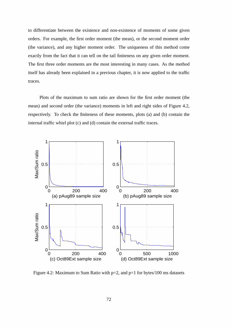
to differentiate between the existence and non-existence of moments of some given

orders. For example, the first order moment (the mean), or thesecond moment order

(the variance), and any higher moment order. The uniquenessof this method come

exactly from the fact that it can tell on the tail finiteness onany given order moment.

The first three order moments are the most interesting in manycases. As the method

itself has already been explained in a previous chapter, it is now applied to the traffic

traces.

Plots of the maximum to sum ratio are shown for the first order moment (the

mean) and second order (the variance) moments in left and right sides of Figure 4.2,

respectively. To check the finiteness of these moments, plots (a) and (b) contain the

internal traffic whiel plot (c) and (d) contain the external traffic traces.

0 200 4000

0.5

1

Max

/Sum

rat

io

(a) pAug89 sample size0 200 400

0

0.5

1

(b) pAug89 sample size

0 200 4000

0.5

1

(c) Oct89Ext sample size

Max

/Sum

rat

io

0 500 10000

0.5

1

(d) Oct89Ext sample size

Figure 4.2: Maximum to Sum Ratio with p=2, and p=1 for bytes/100 ms datasets

72

For the first order moment (the mean), the internal traffic traces produce a ratio

that goes quickly to zero which suggests the mean is finite. Atthe same time, the

external traffic traces produce a ratio that goes to zero but with slower rate. This shows

that internal traffic traces have their means finite. The sameapplies to the case of the

external traffic despite the slow convergence to zero in the latter case.

Another interesting case concerns the second order moment (the variance). It is

shown in the second column of the above mentioned figure. In this case it is remarked

that the internal traffic ratio goes slowly to zero which means that its second order

moment is finite. The external traffic traces have this max/sum ratio slowly approaching

zero but in a very slow rate. Note that for the internal traffic400 values are sufficient

to reach that conclusion, while in the other case more than 1000 values and still the

convergence to zero is slow compared to the internal one. Whatis remarked from this

tool is in line with what is observed earlier from the simple graphs for the external

traffic and in particular for the external traffic trace Oct89Ext. The high fluctuations

show that there is a strong presence of heavy tail distributions.

4.1.4 Gumbel Plot

Gumbel distribution plays a central role in determining thetype of distribution that

data follow within EVT three distribution families. Its role is similar to that of the

normal distribution in classical statistics. Gumbel plot is one of the earliest extreme

value method used by engineers and risk analysts [44]. As defined earlier, it is a plot

of the data against theoretical Gumbel quantile and is essentially used to check the

heavy tail property of the proposed distribution. It helps in distinguishing whether

data can be modeled as coming from a Gumbel distribution or from a distribution with

heavier/lighter tail than Gumbel tail.

In Figure 4.3, Gumbel plot is produced for internal traffic inplot (a) and for

the external traffic in plot (b). In plot (a), two portions from two internal traces are

selected. The internal traces, which are based on the pAug89internal one, are grouped

into blocks of 10 observations each. That translates into 1 second for each block when

73

maxima are taken. The plots for internal traces are not linear. They show an upward

curvature. Such behavior indicates that maxima are distributed with tail lighter than

Gumbel. The same as saying maxima from internal traces are distributed as Weibull

type. It is also known that Weibull distribution corresponds to a GEV distribution

with a negative shape parameter [21]. However, the curvature is not very pronounced

suggesting that a Gumbel might be a possible candidate for this internal traffic maxima

traces.

0 2 4 6 8 10

x 104

−2

−1

0

1

2

3

4

5

6

Gumb

el qu

antile

s

(a) maxima series in 1 second interval for internal traffic

0 1000 2000 3000 4000 5000 6000−2

−1

0

1

2

3

4

5

6

Gumb

el qu

antile

s

(b) maxima series in 1 second interval for external traffic

Figure 4.3: Gumbel probability plot of the internal (a) and external(b) traffic

Gumbel plot for external traffic shows a different behavior.It has a downward

curvature which suggests a distribution with a tail heavierthan Gumbel. In Extreme

Value Theory, it means a distribution of the maxima of external traffic traces that fol-

lows Frechet distribution. As in the financial and insurancemarket, Frechet distribution

or equivalently GEV with positive shape parameter is a common distribution [29].

74

Similar observations are made using the mean excess plot as well. To have a clear

cut, the estimation of the parameters is thus needed. The estimation of the parameters

will reveal more information. Only then these observationswill either be confirmed or

put to doubt. However, these informed guesses from Gumbel plots and Maximum to

Sum ratio along with records give some sense of assurance in the applicability of the

EVT analysis. So it can be considered as safe to jump to the estimation of the parameter

for the two proposed models, the GEV and the GPD.

Next, the implementation of the two core models for the extremes will take place.

Parameters will be estimated and the fit will be assessed. However, estimating and

checking the model parameters requires some software as expected. Surprisingly, most

of the standard or well known statistics software (SAS, SPSS) lack appropriate pack-

ages for extremes implementation. However, some speciallydesigned programs just for

the purpose are recently available and others are being developed by the research com-

munity. The Extremes Toolkit (extRemes) which is built on R statistical programming

platform is just one example. MATLAB also has included some extreme distributions

functions in its 2008 edition, but it is limited and far from complete. For this reason, a

combination of R and MATLAB has been used to carry out the analysis. The data also

has to be exported/imported to use the capabilities of one software or the other.

We used both software interchangeably in the analysis of data. Sometimes data

need to be exported from one R to MATALAB or vice versa. However, no loss of data

occurred in the process.

4.2 Predicting Bursts using GEV

The GEV distribution emerges as the limiting distribution of a sequence of maxima

(minima) of a random variable [37, 29]. This random variablecan be any traffic quantity

of interest. It may refer to file sizes, connection duration,throughput, packet count,

or bytes count. For the purpose of this study the bytes count data have been used.

Meanwhile, bursts in the GEV case are considered to be the block maxima taken in

appropriate block size.

75

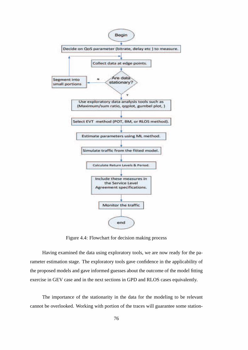
Figure 4.4: Flowchart for decision making process

Having examined the data using exploratory tools, we are nowready for the pa-

rameter estimation stage. The exploratory tools gave confidence in the applicability of

the proposed models and gave informed guesses about the outcome of the model fitting

exercise in GEV case and in the next sections in GPD and RLOS cases equivalently.

The importance of the stationarity in the data for the modeling to be relevant

cannot be overlooked. Working with portion of the traces will guarantee some station-

76

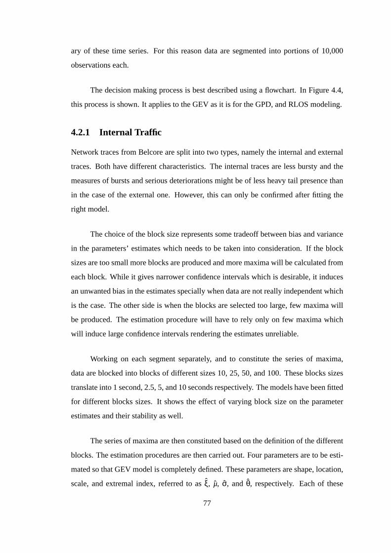
ary of these time series. For this reason data are segmented into portions of 10,000

observations each.

The decision making process is best described using a flowchart. In Figure 4.4,

this process is shown. It applies to the GEV as it is for the GPD, and RLOS modeling.

4.2.1 Internal Traffic

Network traces from Belcore are split into two types, namely the internal and external

traces. Both have different characteristics. The internal traces are less bursty and the

measures of bursts and serious deteriorations might be of less heavy tail presence than

in the case of the external one. However, this can only be confirmed after fitting the

right model.

The choice of the block size represents some tradeoff between bias and variance

in the parameters’ estimates which needs to be taken into consideration. If the block

sizes are too small more blocks are produced and more maxima will be calculated from

each block. While it gives narrower confidence intervals which is desirable, it induces

an unwanted bias in the estimates specially when data are notreally independent which

is the case. The other side is when the blocks are selected toolarge, few maxima will

be produced. The estimation procedure will have to rely onlyon few maxima which

will induce large confidence intervals rendering the estimates unreliable.

Working on each segment separately, and to constitute the series of maxima,

data are blocked into blocks of different sizes 10, 25, 50, and 100. These blocks sizes

translate into 1 second, 2.5, 5, and 10 seconds respectively. The models have been fitted

for different blocks sizes. It shows the effect of varying block size on the parameter

estimates and their stability as well.

The series of maxima are then constituted based on the definition of the different

blocks. The estimation procedures are then carried out. Four parameters are to be esti-

mated so that GEV model is completely defined. These parameters are shape, location,

scale, and extremal index, referred to asξ, µ, σ, and θ, respectively. Each of these

77

parameters have a different effect on the distribution. Thelocation parameterµ has the

effect of shifting the distribution either to the left or to the right in the horizontal axis.

The scale parameterσ determines the stretch of the shape of the distribution. It either

stretch it or compress it. The shape parameter which is an important one determines

the type of the distribution tail, either light or heavy. Theextremal indexθ, which ac-

counts for the dependency in the data, will adjust the above parameters. That follows

because in the dependence case these estimates tend to overestimate the true values of

the parameters.

Classically, only the first three parameters are estimated. The extremal index

parameter is being included to measure the degree of dependency in the data since

the data are supposed to be i.i.d. The estimation procedureshave been carried out in

MATLAB using the Maximum Likelihood procedure.

The segments of the internal traffic traces along with the simulated results based

on the fractional Gaussian noise (H=0.78) model are summarized in Table 4.3.

Data in this table are merely a subset from the data that are summarized in Table

4.1. They contain segments of the data so that the stationarity assumption remains valid.

For example, the trace pAug1to5k is extracted from the tracepAug89 starting from the

first observation to the five thousands one. The same convention is followed in the other

data set with the exception of fafgn which is the a simulated fractional Gaussian noise.

Table 4.3: Summary Statistics of Internal Traffic TracesDataset size Maximum Mean Variance Std Median Modefafgn 9999 99.0970 20.3419 233.1899 15.2706 17.1902 0.0033

pAug1to5k 5000 92524 18022 210470000 14507 13920 4866pAug5to10k 5001 85387 14796 209710000 14481 10471 192pOct1kto5k 4000 87015 29858 222440000 14914 29889 22380pOct5kto10k 5000 90706 29712 221850000 14894 29983 8690

The Belcore traces are taken as bytes per 0.1 second. The length of each segment

is set to eight minutes to guarantee some sort of stationarity in the data. However, in

practice, this choice can be relaxed once the stationarity assumption is verified. Some

78

of the above traces are plotted in Figure 4.5 where the four traces look similar and

equally bursty.

0 2000 4000 60000

2

4

6

8

10x 10

4

(b) Time scale for pOct1kto5k

Byt

es c

ount

0 2000 4000 60000

2

4

6

8

10x 10

4

(c) Time scale for pAug1to5k

Byt

es c

ount

0 2000 4000 60000

2

4

6

8

10x 10

4

(d) Time scale for pAug5to10k

Byt

es c

ount

0 2000 4000 60000

20

40

60

80

100

(a) Time axis for fgn

Byt

es c

ount

Figure 4.5: Internal traffic traces

The estimation procedure has been carried out for all the above traces. The esti-

mates of the shape parameter of the examined datasets of internal traces are tabulated

in Table 4.4. These estimates are based on the ML method. The table includes only

the shape parameter, not the location, scale or the extremalindex. This is because the

shape parameter is an important factor which will determinethe shape of the resulting

GEV distribution. The other parameters do not alter the shape of the distribution in any

significant way.

Knowing that the choice of the block size is crucial and important, estimates are

calculated for different block sizes of 10, 20, 30, among others. This will allow for

judgment of the stability of the shape parameter estimate. It also shows the effect of

different blocks sizes on the sign of the estimate. However,it is to be noticed that the

79

maximum of the block of size 10 is equivalent to saying the maximum in 1 second

period. This is because the traces here have one observationfor every 0.1 second.

A first glance into the estimates reveals that the shape parameter has predomi-

nately values less than zero in all the selected bock sizes choice. This is equivalent

to saying that the internal traffic trace distribution is in the domain of attraction of the

Weibull distribution. That is, the maximum from the internal traces are following the

GEV distribution with a negative shape parameter.

A closer look reveals a tendency on the shape parameter to have larger negative

values with the increasing the block sizes of 10 to 20 for example. The case of the

block size of 10 is one of interest. When the maxima are taken inblocks of sizes 10, it

is possible that these maxima be modeled as coming from Gumbel distribution rather

than Weibull distributions. The shape parameter assumes values very close to zero that

sometimes traces fall in the domain of attraction of Gumbel distribution. A perfect

example is the trace pAug1to5k at the 10 block size level where the estimate is -0.04

(0.04) which gives a 95 confidence interval of [-0.08 0.00].

A major concern in fitting GEV distribution is to know the typeof the distribution

to be fitted and the shape of the parameter. These results havethe meaning that bursts

and serious deteriorations in the internal traffic have an upper limit that it would not

exceed. This comes from the fact that Weibull distribution has a finite upper tail. We

refer to Figure 3.2 on Page 39 for a look into the different possible tail shapes.

Having a finite upper end of bursts and serious deteriorations in the case of in-

ternal traffic is something unexpected. The reason for this finiteness is that often time

Table 4.4: Shape parameter estimatesξ for different block sizesDataset n=10 n=20 n=30 n=40 n=50 n=75 n=100

fafgn -0.09(0.02) -0.11(0.03) -0.10(0.04) -0.15(0.04) -0.12(0.05) -0.09(0.07) -0.14(0.07)pAug5to10k -0.06(0.04) -0.21(0.05) -0.24(0.06) -0.30(0.06) -0.29(0.07) -0.33(0.08) -0.42(0.09)pAug1to5k -0.04(0.04) -0.14(0.04) -0.16(0.05) -0.13(0.06) -0.15(0.07) -0.17(0.08) -0.24(0.10)pOct1kto5k -0.11(0.03) -0.02(0.06) -0.10(0.09) -0.15(0.09) -0.22(0.12) -0.36(0.14) -0.51(0.15)pOct5kto10k -0.11(0.03) -0.05(0.05) 0.02(0.09) -0.18(0.09) -0.28(0.09) -0.36(0.09) -0.45(0.08)

80

network resources and equipments have themselves limited bandwidth. They have also

a predefined set of applications in which the performance of the internal network can

be bounded by the set of applications behavior.

These results of internal traffic bursts and serious deteriorations distribution are

believed to be strongly related to Norros results on the behavior of a buffer that is

fed by the fractional Brownian motion (fBm) traffic. fBm is also the type of traffic

that has been simulated here for the internal traffic. It is thus strongly related to the

results shown here bearing in mind that internal traffic simulation is FGN which is the

incremental process of fBm. It is also worth noting that Norros arrived to this result

using queuing theory, here it is arrived at using extreme value theory.

Graphical tools are used to assess the quality of fit . The simulated data shows a

good fit. There is a match between the model and empirical data. Both other internal

traces showed a good fit as well, with a light deviation due to mostly the statistical vari-

ability. An example of the cumulative distribution function for the model and empirical

data for the fafgn data with blocks of size 10 is shown in Figure 4.6.

30 40 50 60 70 80 900

0.1

0.2

0.3

0.4

0.5

0.6

0.7

0.8

0.9

1

Data

Cum

ulat

ive

prob

abili

ty

fafgnb20 datafit2

Figure 4.6: CDF of the fitted distribution and the empirical one

An almost perfect fit is produced with the block sizes of 20, 30, 40. The same

81

plot for the other real Belcore traces produces plots that have some deviations. This is

illustrated in Figure 4.7.

2 3 4 5 6 7 8 9

x 104

0

0.1

0.2

0.3

0.4

0.5

0.6

0.7

0.8

0.9

1

Data

C

umul

ativ

e pr

obab

ility

pAug1to5kb30 data fit7pAug1to5kb75 data fit 8

Figure 4.7: CDF for two internal traces with different block sizes

Assessment of the quality of the fitted models is performed using four plots, namely:

qqplot, mean excess plot, probability plot, and the histogram. These plotting tools

are found in the package ’extRemes’ which operates under the statistical computing

environment R.

In Figure 4.8, the four diagnostic plots are shown for the internal trace pOct89

with blocks sizes of 30 observations. The probability plot shows a good alignment to

the straight line while qq-plot shows a little deviation in the upper right corner of the

plot. The return level plot has some points that deviate fromthe theoretical behavior

which is represented by the solid line. The same trace shows abetter fit when produced

in greater block sizes of 75. This is shown in Figure 4.9. The qq-plot shows perfect

alignment. Return level plot also shows points that are perfectly aligned.

The deviation of the model and empirical observations is remarked through other

internal traces. When viewed in a very small block size of 10, for example, a deviation

is observed. However, with larger block sizes the fitting tends to be almost perfect. It

82

can be concluded that GEV model provides better fits for internal traffic when blocks

are large enough.

4.2.2 External Traffic

External traffic has patterns than are different from internal traffic. This has been ob-

served from the exploratory analysis conducted earlier in Section 4.1. The fitting tech-

niques will be conducted for the External traffic traces in the following.

External traffic data that will be looked into in details are plotted in Figure 4.10.

Their descriptive statistics are tabulated in Table 4.5. Itcan be seen from both plots

and the tables that the external traffic is burstier than the internal traffic. However,

estimating the parameters of the GEV model is the primary concern here.

0.0 0.2 0.4 0.6 0.8 1.0

0.0

0.4

0.8

Probability Plot

Empirical

Mod

el

4e+04 7e+04 1e+05

4000

070

000

Quantile Plot

Model

Em

piric

al

4000

080

000

1200

00

Return Period

Ret

urn

Leve

l

0.1 1 10 100 1000

Return Level Plot Density Plot

z

f(z)

40000 60000 80000

0.0e

+00

2.0e

−05

Figure 4.8: Diagnostics for pOct89 trace with block size of 30

83

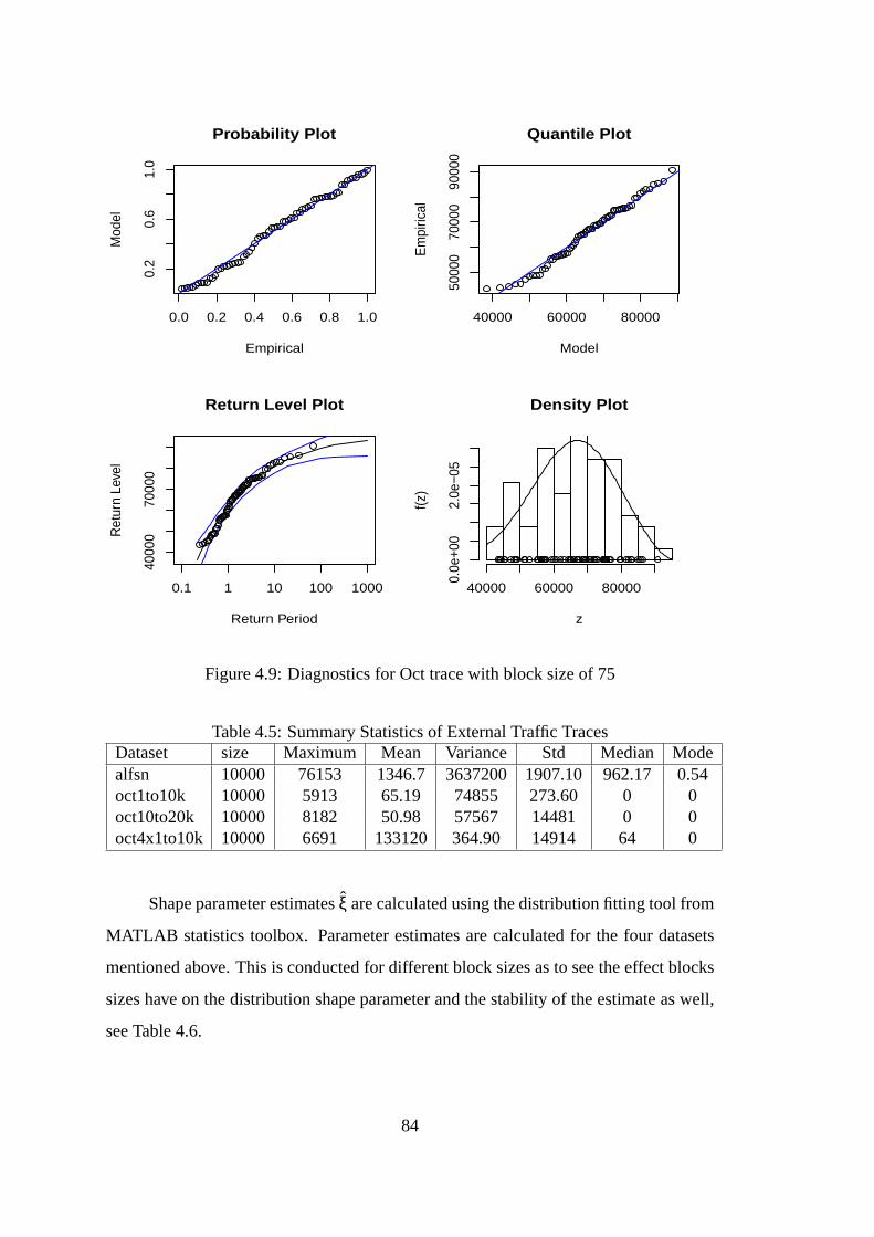
0.0 0.2 0.4 0.6 0.8 1.0

0.2

0.6

1.0

Probability Plot

Empirical

Mod

el

40000 60000 80000

5000

070

000

9000

0

Quantile Plot

Model

Em

piric

al

4000

070

000

Return Period

Ret

urn

Leve

l

0.1 1 10 100 1000


z

f(z)

40000 60000 80000

0.0e

+00

2.0e

−05

Figure 4.9: Diagnostics for Oct trace with block size of 75

Table 4.5: Summary Statistics of External Traffic TracesDataset size Maximum Mean Variance Std Median Modealfsn 10000 76153 1346.7 3637200 1907.10 962.17 0.54oct1to10k 10000 5913 65.19 74855 273.60 0 0oct10to20k 10000 8182 50.98 57567 14481 0 0oct4x1to10k 10000 6691 133120 364.90 14914 64 0

Shape parameter estimatesξ are calculated using the distribution fitting tool from

MATLAB statistics toolbox. Parameter estimates are calculated for the four datasets

mentioned above. This is conducted for different block sizes as to see the effect blocks

sizes have on the distribution shape parameter and the stability of the estimate as well,

see Table 4.6.

84

0 5000 100000

20

40

60

80

(a) Time axis for LFSN

Byt

es c

ount

0 5000 100000

2000

4000

6000

(b) Time axis for oct1to10k

0 5000 10000 150000

2000

4000

6000

8000

10000

(c) Time axis for oct10to20k

Byt

es c

ount

0 5000 100000

2000

4000

6000

8000

(d) Time axis for oct4x1to10k

Figure 4.10: Plot of External traffic traces

Table 4.6: Shape parameter estimatesξ for External TrafficDataset 10 20 30 40 50 75 100

alfsn 0.41(0.02) 0.53(0.04) 0.46(0.05) 0.51(0.06) 0.56(0.08) 0.59(0.10) 0.52(0.11)oct1to10k 5.01(NA) 0.75(0.06) 0.69(0.06) 0.68(0.06) 0.74(0.07) 0.75(0.08) 1.04(0.13)

oct10to20k 5.21(NA) 0.63(0.05) 0.63(0.05) 0.63(0.05) 0.69(0.06) 0.72(0.08) 0.75(0.09)oct4x1to10k 0.83(0.04) 0.78(0.06) 0.62(0.09) 0.52(0.10) 0.40(0.10) 0.26(0.11) 0.24(0.12)

Unlike internal traffic where estimates are predominately less than zero, here it

is seen that the parameter estimates are mostly positive. This is true through all the

different choices of blocks and the different external traces. The estimation procedure

based on ML method has converged for all the estimates exceptfor the block of size 10.

It did not converge for the second and third traces, oct1to10k and oct10to20k. This is

due to the structure of these particular traces where many values are zero and it follows

that small blocks size of 10 would produce nothing but zeros as well.

The positive shape parameter has the meaning that block maxima from external

traffic traces follow a GEV distribution that is heavy tailed. This is equivalent to Frechet

distribution. Thus the external traffic traces fall in the domain of attraction of Frechet

distribution. This is because of the very heavy tail marginal distribution of the original

traces. It was predicted to be so by the exploratory data analysis conducted at the

85

beginning of this chapter.

Now, we look into the stability of the parameter estimates. It is remarked that

estimates of the shape parameter for the first three traces are stable to some extent.

They assume values in the range of 0.5 to 0.77 in most cases. Only one case happens

in the second trace of blocks of size 100 where it exceeds 1. The stability of the shape

parameter in these traces is clear. Only trace [octx1to10k]shows a decrease in the value

of the parameter with increase in the block size from 10, 20 to. . . 100.

As for the checking of the model, empirical CDFs of the traces are plotted along

with the theoretical CDF based on the fitted models. This is done in Figure 4.12 and

Figure 4.11. In Figure 4.12, two theoretical CDFs are plottedbased on model fits along

with three empirical CDF for the traces. There is a close matchbetween the empirical

and theoretical one in both cases. A little deviation is remarked and mostly is due to

the statistical variability. In Figure 4.11, the empiricalCDF is plotted for fitted model

based on the simulated traffic trace LFSN. The match in this case is just seen to be

perfect.

1 2 3 4 5 6 7

x 104

0

0.1

0.2

0.3

0.4

0.5

0.6

0.7

0.8

0.9

1

Data

Cum

ulat

ive

prob

abili

ty

lfsn20 data fit2lfsn100 data fit7

Figure 4.11: Two cdf of different fit to the LFSN dataset

However, as discussed in the model fitting and diagnostic context, one should not

rely on one tool or plot as it may be possible to be misled. Morediagnostics of the

86

model are then carried out using ExtRemes package in R computing environment.

0 1000 2000 3000 4000 5000 6000 7000 80000

0.1

0.2

0.3

0.4

0.5

0.6

0.7

0.8

0.9

1

Data

Cum

ulat

ive

prob

abili

ty

oct1to10kb50 data fit 9oct10to20kb50 datao4ct1to10kb100 data fit 14

Figure 4.12: Cumulative Distribution Function of some fits and empirical ones

The diagnostic plots are shown in two figures for the Belcore trace and the sim-

ulated LFSN trace as well. In Figure 4.13, the plots are for the original traces based

on Belcore data. There is almost no doubt about the quality of fit for the model to the

empirical data. The points are perfectly aligned through the probability plots and the

q-q plot. The return plot is the typical one for the data that are heavy tailed.

Looking at the Figure 4.14, which shows diagnostic plots forGEV fit of LFSN

taken at blocks of , the picture is not equally rosy as the previous case. Here, a clear

deviation is shown by the plots and in particular that of the qqplot which is not revealing

at all. This is a bit striking if compared to the almost perfect fit when looked at it

through the CDF in Figure 4.11. A possible explanation is thatthis deviation is due

to some extent to the very strong dependence in the LFSN simulated traces compared

to the empirical ones. However, the other Belcore traces are all showing quality of fit

similar to each other. Thus, it leaves no doubt about the applicability of the model.

Return level and return period are two prediction tools basedon the fitted GEV

model. It is the inverse of the GEV model. It extrapolates in the high quantile and can

87

answer questions like how large a burst might be in the next interval? And what amount

of time is needed for bursts of such magnitude to happen again?

Thus, traffic traces both the internal and external are modeled using the GEV

model. It is a straightforward exercise once the exploratory data analysis is done thor-

oughly and the stationarity of the data is verified.

4.3 Predicting Bursts using GPD

GEV model has been criticized for its not so efficient use of the available data as it picks

only one data point from each block, the maxima, to model [21]. Clearly, this could

result in some loss of information since all the other data ina given block become

irrelevant no matter how close to the block maximum they might be.

0.0 0.2 0.4 0.6 0.8 1.0

0.2

0.6

1.0

Probability Plot

Empirical

Mod

el

40000 60000 80000

5000

070

000

9000

0

Quantile Plot

Model

Empi

rical

4000

070

000

Return Period

Ret

urn

Leve

l

0.1 1 10 100 1000


z

f(z)

40000 60000 80000

0.0e

+00

2.0e

−05

Figure 4.13: Diagnostics plots for oct1to10kb75 fit

88

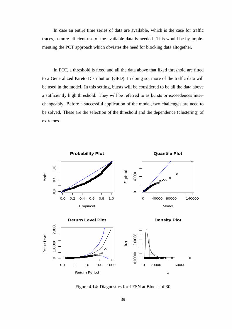
In case an entire time series of data are available, which is the case for traffic

traces, a more efficient use of the available data is needed. This would be by imple-

menting the POT approach which obviates the need for blocking data altogether.

In POT, a threshold is fixed and all the data above that fixed threshold are fitted

to a Generalized Pareto Distribution (GPD). In doing so, more of the traffic data will

be used in the model. In this setting, bursts will be considered to be all the data above

a sufficiently high threshold. They will be referred to as bursts or exceedences inter-

changeably. Before a successful application of the model, two challenges are need to

be solved. These are the selection of the threshold and the dependence (clustering) of

extremes.

0.0 0.2 0.4 0.6 0.8 1.0

0.0

0.4

0.8

Probability Plot

Empirical

Mod

el

0 40000 80000 140000

040

000

Quantile Plot

Model

Empi

rical

010

0000

2500

00

Return Period

Ret

urn

Leve

l

0.1 1 10 100 1000


z

f(z)

0 20000 60000

0.00

000

0.00

008

Figure 4.14: Diagnostics for LFSN at Blocks of 30

89

As for the dependence or clustering of extremes, it is well known that traffic is

self-similar which is highly correlated. Such correlationmeans that bursts are not truly

independent and some degree of dependency do exist in between them. Thus, if a burst

occurred now, it would soon be followed by another burst. This is called clustering of

extremes and this dependency structure violates the assumption of the model. It follows

that it puts in doubt any application of the model in that case. Any application of POT

analysis in the dependency presence may prove invalid and atbest erroneous.

However, this problem has been overcome by some de-clustering technique which

filters dependent observations. It produces observations that are approximately inde-

pendent without altering their values.

Identification of clusters is done by selecting a threshold (not necessary the one

used in estimating GPD parameters). Then it defines consecutive exceedences of this

threshold to belong to the same cluster. The cluster ends when a number ofk observa-

tions fall below the above selected threshold. The next cluster then starts with the first

exceedences ofu.

Selection ofu andk is done by the practitioner. Cautions selection is to be made

since a trade off similar to the one in block selection in GEV modeling is present. Ifk

is too small, the independence between clusters will be put into doubt, while ifk is too

large then exceedences that would have been otherwise put indifferent clusters will be

regrouped and put in the same cluster.


As mentioned earlier, a primary step in applying a GPD model is to select an appropriate

threshold. Noting that for the model to be valid, a sufficiently high threshold needs to

be selected. The following mean excess plots are produced for the internal traces as to

select an appropriate threshold for the GPD modeling, see Figure 4.15.

Ideally, the threshold is selected after a sudden change in the mean excess plot,

after which it becomes linear. However, it is not always easyto determine this point of

90

0 2 4 6 8 10

x 104

0

0.5

1

1.5

2x 10

4

(a) Threshold pAug5to10kM

ean

Exc

ess

0 2 4 6 8 10

x 104

0

0.5

1

1.5

2x 10

4

(b)Threshold pAug5to10k

Mea

n E

xces

s

0 2 4 6 8 10

x 104

0

1

2

3x 10

4

(c) Threshold pOct5kto10k

Mea

n E

xces

s

0 20 40 60 80 1000

10

20

30

(d) Threshold fafgn

Mea

n E

xces

s

Figure 4.15: Mean excess plots for the internal traces

Table 4.7: Internal Traffic GPD resultsTrace Threshold ξ Extremal Ind. Clusters Run lengthfafgn 54.57 -0.15(0.05) 0.79(0.70,0.91) 237 2pAug1to5k 53374.90 -0.18(0.10) 0.65(0.52,0.82) 80 5pAug5to10k 57432 -0.20(0.13) 0.520(0.38,0.75) 51 11pOct1kto5k 60926 -0.38(0.08) 0.46(0.35,0.62) 53 8pOct5kto10k 60290 60290 0.36(0.26,0.50) 62 9

change and these plots are difficult to interpret precisely.But still, they are better than

guesswork. The selected threshold values are shown in the first column in Table 4.7.

As mentioned earlier, the extremal index is a measure of the dependence. It pro-

vides a mean to adjust the modeling parameters so that the dependency in the data can

be accounted for. Figure 4.16 shows the extremal index estimate plotted against the

threshold for the traffic trace fafgn. The plot shows extremal index assuming values

around 0.8 which suggest that the extremes tend to happen in clusters. The other ex-

tremal indexes for other internal traces are showing similar behavior and their values

are shown in Table 4.7.

Clustering is closely related to the extremal indexθ. If θ = 1, then there is no

clustering in the data. Data can be considered independent and GPD parameters can

be readily estimated. However, ifθ < 1, which is the case in many of the traffic data,

91

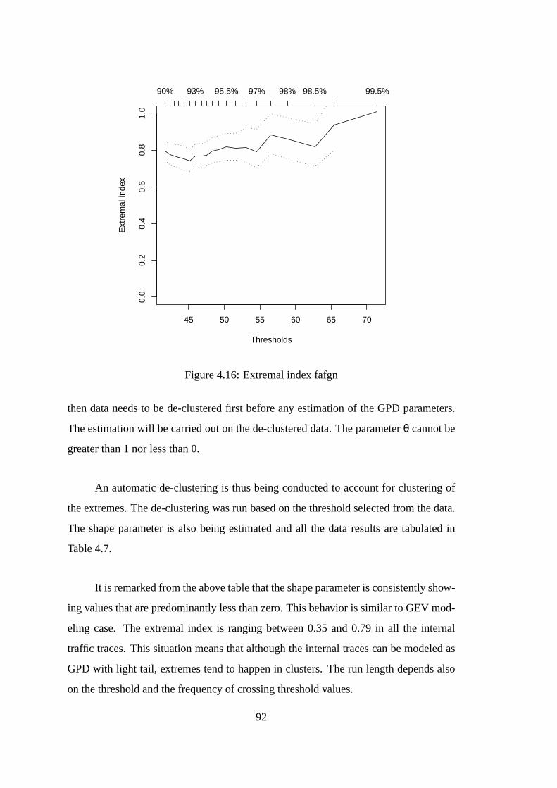
45 50 55 60 65 70

0.0

0.2

0.4

0.6

0.8

1.0

Thresholds

Ext

rem

al in

dex

90% 93% 95.5% 97% 98% 98.5% 99.5%

Figure 4.16: Extremal index fafgn

then data needs to be de-clustered first before any estimation of the GPD parameters.

The estimation will be carried out on the de-clustered data.The parameterθ cannot be

greater than 1 nor less than 0.

An automatic de-clustering is thus being conducted to account for clustering of

the extremes. The de-clustering was run based on the threshold selected from the data.

The shape parameter is also being estimated and all the data results are tabulated in

Table 4.7.

It is remarked from the above table that the shape parameter is consistently show-

ing values that are predominantly less than zero. This behavior is similar to GEV mod-

eling case. The extremal index is ranging between 0.35 and 0.79 in all the internal

traffic traces. This situation means that although the internal traces can be modeled as

GPD with light tail, extremes tend to happen in clusters. Therun length depends also

on the threshold and the frequency of crossing threshold values.

92

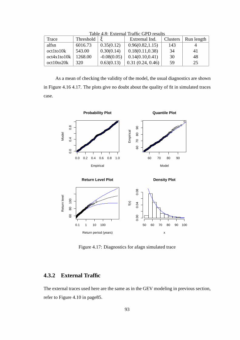
Table 4.8: External Traffic GPD resultsTrace Threshold ξ Extremal Ind. Clusters Run lengthalfsn 6016.73 0.35(0.12) 0.96(0.82,1.15) 143 4oct1to10k 543.00 0.30(0.14) 0.18(0.11,0.38) 34 41oct4x1to10k 1268.00 -0.08(0.05) 0.14(0.10,0.41) 30 48oct10to20k 320 0.63(0.13) 0.31 (0.24, 0.46) 59 25

As a mean of checking the validity of the model, the usual diagnostics are shown

in Figure 4.16 4.17. The plots give no doubt about the qualityof fit in simulated traces

case.

0.0 0.2 0.4 0.6 0.8 1.0

0.0

0.4

0.8

Probability Plot

Empirical

Mod

el

60 70 80 90

6070

8090

Quantile Plot

Model

Em

piric

al

6080

100

Return Level Plot


Ret

urn

leve

l

0.1 1 10 100

Density Plot

x

f(x)

50 60 70 80 90 100

0.00

0.04

0.08

Figure 4.17: Diagnostics for afagn simulated trace


The external traces used here are the same as in the GEV modeling in previous section,

refer to Figure 4.10 in page85.

93

The need of the mean excess plot was mentioned previously in the internal traffic

case. Figure 4.18, shows four mean excess plots for the external traces. These mean

excess plots have an upward slope which is fundamentally different from the downward

direction of the internal traces case in Figure 4.15 page 91.Apart from acting as a mean

for selecting a threshold, the upward in the mean excess plots shows that data comes

from a heavy tail distribution. This is a typical behavior for data from the financial and

insurance data.

0 1 2 3 4

x 104

0

1

2

3x 10

4

(a) Threshold alfsn

Mea

n E

xces

s

0 2000 4000 60000

500

1000

1500

(b) Threshold oct1to10k

Mea

n E

xces

s

0 2000 4000 60000

1000

2000

3000

(c) Threshold oct10to20k

Mea

n E

xces

s

0 2000 4000 60000

500

1000

1500

(d) Threshold oct4x1to10k

Mea

n E

xces

s

Figure 4.18: Mean Excess plot for external traces

However, the meplot for the trace alfsn shows a net upward trend. This coincides

with the theory. It comes very clear as alfsn itself is a simulated trace. Plot (c) of

oct10to20k is showing an upward trend which comes obvious despite decline around

the 2kb value. In contrast to plot (d) when a cyclic trend is present with overall positive

slope. This cyclic trend is vexing but it is due to the silent periods in the trace. It can

be understood also from the way the mean excess plot is calculated since it averages

the data above a given point. In the presence of a lot of silentperiods, some of the

exceedences are divided by more points that do not contribute to the sum.

94

0.0 0.2 0.4 0.6 0.8 1.0

0.0

0.4

0.8

Probability Plot

Empirical

Mod

el

0 10000 30000 50000

040

000

Quantile Plot

Model

Em

piric

al

0e+

004e

+05

Return Level Plot


Ret

urn

leve

l

0.1 1 10 100 1000

Density Plot

x

f(x)

0 20000 40000 60000 80000

0e+

004e

−04

8e−

04

Figure 4.19: Diagnostics plots of alfsn with u=1850,ξ=0.41(0.03)

4.4 Predicting Bursts usingr-largest order statistics

For the purpose of completeness, ther-largest order statistics as a model is included

in bursts analysis and prediction. This model is half way between the block maxima

method and the peaks over threshold method. As in the BM method, traffic data are

segmented into blocks and then from each block ther-largest orders are computed and

used to be fit to the model.

The data used in this consisted of both internal and externaltraces as earlier. The

data have been transformed into a vector in such a way that from each block, seven

highest values are selected and a new vector consisting of 7 values for each block is

constructed. This is done through a simple MATLAB routine.

95


The exploratory phase is the same as the previous section so it is not going to be re-

peated. The parameters of the model are estimated for eachr = 1, r = 2, . . . , r = 7.

This is to judge the accuracy of the estimates by the mean of their confidence intervals.

These results are tabulated in Table 4.9.

In the table, parameter estimates for internal traces of fgnand pOct5kto10k are

presented. The trace fgn in the top section of table is segmented into blocks of size 40

in the left side of the table and to blocks of size 75 to the right side of the table. For the

fgn trace in 40 size blocks the estimates of the shape parameter are mostly positive as

was the case in the GEV model.

0.0 0.2 0.4 0.6 0.8 1.0

0.2

0.6

1.0

Probability Plot

Empirical

Mod

el

2000 3000 4000 5000 6000 7000

2000

5000

8000

Quantile Plot

Model

Em

piric

al

1000

030

000

Return Level Plot


Ret

urn

leve

l

0.1 1 10 100 1000

Density Plot

x

f(x)

2000 4000 6000 8000

0e+

004e

−04

Figure 4.20: Diagnostics plots oct10to20k with u =2000

96

Table 4.9: RLOS Parameters for internal Traffic TracesInternal Traffic

Trace fafgn, block size 40 fafgn, block size 75par ξ σ µ ξ σ µr=1 -0.100(0.038) 05.600(0.270) 34(0.39) -0.120(0.057) 5.34(0.36) 42(0.52)r=2 -0.116(0.027) 05.492(0.181) 37(0.33) -0.124(0.042) 5.10(0.23) 44(0.43)r=3 -0.153(0.022) 05.790(0.160) 40(0.32) -0.175(0.034) 5.29(0.19) 47(0.41)r=4 -0.177(0.020) 06.235(0.157) 43(0.33) -0.183(0.029) 5.71(0.19) 50(0.43)r=5 -0.173(0.017) 06.986(0.167) 46(0.36) -0.185(0.027) 6.39(0.21) 54(0.46)r=6 -0.160(0.015) 08.140(0.189) 51(0.42) -0.162(0.023) 7.52(0.24) 57(0.54)r=7 -0.120(0.020) 10.220(0.280) 56(0.52) -0.122(0.027) 9.55(0.36) 63(0.67)

Trace pOct5kto10k, Block size 40 pOct5kto10k, Block size 75par ξ σ µ ξ σ µr=1 0.095(0.062) 6298(473) 39820(620) 0.095(0.062) 6298(473) 39820(620)r=2 0.016(0.041) 6837(359) 43679(578) 0.016(0.041) 6837(359) 43679(578)r=3 0.016(0.037) 7505(381) 47454(598) 0.016(0.037) 7505(381) 47454(598)r=4 -0.017(0.028) 7134(267) 48977(515) -0.017(0.028) 7133(267) 48977(515)r=5 -0.013(0.033) 8578(390) 53702(611) -0.013(0.033) 8578(390) 53702(611)r=6 -0.036(0.030) 9195(433) 57063(657) -0.036(0.033) 9195(433) 57062(657)r=7 -0.089(0.024) 8638(266) 57964(603) -0.089(0.024) 8638(266) 57964(603)

However, running fromr = 1, tor = 7, it is seen that the precision of the estimates

change with increasing value ofr. The least confidence interval (preferable) is seemed

to be inr = 6(0.015), while for the scale parameter it happens atr = 4(0.157) and for

location it is atr = 3(0.32).

When the same fgn trace is blocked in size of 75 blocks, the bestconfidence

interval for the shape parameter happens again atr = 6(0.023). For scale parameter it

is atr = 4(0.19). For location parameter it happens atr = 3(0.41).

For the other internal trace pOct5kto10k, when blocked at blocks of size 40,r = 7

presented the best confidence interval for the shape and scale parameters. The location

has its best estimate atr = 3. Meanwhile, and in the right side of the table where the

trace is blocked at 75 blocks, the best confidence interval for shape and scale was at

r = 7. For the location parameter, it is atr = 4.

The model fitted to many internal traces is showing conformity with the expected

behavior based on the estimates calculated in the above table. As an example, in Figure

4.21, the diagnostics plots are produced for the internal trace fgn with blocks of size

97

0.0 0.2 0.4 0.6 0.8 1.0

0.0

0.4

0.8

Probability Plot

Empirical

Mod

el

50 60 70 80 90

5070

90

Quantile Plot

Model

Empi

rical

1e−01 1e+01 1e+03

5070

90

Return Period

Ret

urn

Leve

l


z

f(z)

40 50 60 70 80 90

0.00

0.02

0.04

Figure 4.21: Diagnostics of fractional Gaussian noise afgntrace at blocks of 75 withr=6

75. The number of orders statistics is taken asr = 6. Clearly, the quantile plot and the

probability plots are showing agreement with the theoretical behavior expected by the

solid line. This good fit with tighter confidence intervals should act a base for all the

prediction calculations using the return level and return periods concepts.


External traffic traces are based on the same traces used in modeling with GEV. As

in the previous cases, GEV and GPD, the shape parameter is predominately positive.

This is a clear indication of the heavy tail property of the distribution of external traffic

bursts and serious deteriorations. Table 4.10 summarizes the parameter estimates for

two traces, one is the simulated trace lsfsn and the other is the one from Belcore. In

the upper left part of Table 4.10, estimates of simulated trace when blocked in 40 are

98

shown. The estimates are littered with NaN for not availabledata for reasons of non

convergence of the Likelihood procedure. However, the bestestimates interval for the

shape parameter and scale parameter are atr = 5(0.033,122,4774). When blocked in

75 blocks, it is atr = 4 that the shape parameter and location parameter are good. It is

at r = 5 for the scale parameter.

Table 4.10: RLOS Parameters for External Traffic TracesExternal Traffic

Trace rlosalfsnb40, block size 40 rlosalfsnb75, block size 75par ξ σ µ ξ σ µr=1 0.507(0.062) 2290(160) 4887(165) 0.587(0.099) 2979(306) 6310(302)r=2 0.572(0.052) 2326(158) 4878(140) 0.822(NaN) 5924(NaN) 8501(NaN)r=3 1.006(NaN) 5081(NaN) 6529(NaN) 1.036(NaN) 7231(NaN) 8770(NaN)r=4 0.979(NaN) 5356(NaN) 6817(NaN) 0.575(0.055) 3158(269) 6375(230)r=5 0.497(0.033) 2149(122) 4774(112) 0.827(0.173) 5947(217) 8468(1428)r=6 0.766(0.301) 4276(2813) 6453(1921) 0.821(NaN) 5912(NaN) 8484(NaN)r=7 0.756(NaN) 4572(NaN) 6777(NaN) 0.893(NaN) 7130(NaN) 9331(NaN)

Trace rlosoct4x1to10kb40, Block size 40 rlosoct4x1to10kb75, Block size 75par ξ σ µ ξ σ µr=1 0.519(0.103) 552(44) 607(46.67) 0.271(0.109) 737(67) 922(79)r=2 0.672(0.081) 675(47) 775(43.63) 0.342(0.101) 824(60) 1157(76)r=3 0.787(0.072) 829(70) 903(48.75) 0.360(0.086) 881(68) 1316(71)r=4 0.803(0.052) 839(64) 926(45.70) 0.452(0.079) 953(85) 1402(71)r=5 0.750(0.039) 781(51) 911(39.34) 0.491(0.065) 925(74) 1376(64)r=6 0.795(0.036) 874(63) 993(46.60) 0.544(0.058) 925(70) 1348(60)r=7 0.761(0.033) 858(60) 1007(45.77) 0.568(0.050) 924(66) 1337(56)

At the bottom side of the table is the other trace oct4x1to10k. In this case as

the previous one for the simulated traces, the shape parameter is also predominately

positive in value. However, the estimates here do converge all of them. In the left side

of the bottom table, the estimate for the trace when blocked at blocks of size 40. There

is a dramatic improvement in the confidence interval going from r = 1 to higher values

of r. As r reaches 7, the best confidence intervals for the shape parameter are produced.

It is at r = 1 the best estimate are shown for the scale. The best estimates happen at

r = 5 for the location parameter.

The right side of the table shows the same information for thetrace blocked at

the 75 size. Both shape and location parameters have their best estimates atr = 7, it is

at r = 2 for the scale parameter.

99

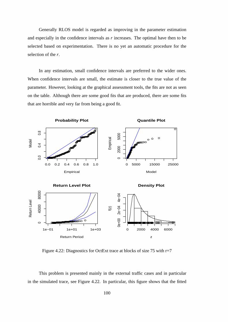
Generally RLOS model is regarded as improving in the parameter estimation

and especially in the confidence intervals asr increases. The optimal have then to be

selected based on experimentation. There is no yet an automatic procedure for the

selection of ther.

In any estimation, small confidence intervals are preferredto the wider ones.

When confidence intervals are small, the estimate is closer tothe true value of the

parameter. However, looking at the graphical assessment tools, the fits are not as seen

on the table. Although there are some good fits that are produced, there are some fits

that are horrible and very far from being a good fit.

0.0 0.2 0.4 0.6 0.8 1.0

0.0

0.4

0.8

Probability Plot

Empirical

Mod

el

0 5000 15000 25000

020

0050

00Quantile Plot

Model

Empi

rical

1e−01 1e+01 1e+03

040

000

8000

0

Return Period

Ret

urn

Leve

l


z

f(z)

0 2000 4000 6000

0e+0

02e

−04

4e−0

4

Figure 4.22: Diagnostics for OctExt trace at blocks of size 75 with r=7

This problem is presented mainly in the external traffic cases and in particular

in the simulated trace, see Figure 4.22. In particular, thisfigure shows that the fitted

100

model is not working as expected. There is a clear deviation in both the probability

plot and the quantile plot for the theoretical one represented by the solid lines. This

nonconformity is believed to be as a result of some dependency in the data. It is due

in part to the stationarity assumption as well. Thus the RLOS model especially for the

external traces is not working as expected.

4.5 summary

In this chapter, models from Extreme Value Theory have been applied to traffic traces

from Belcore. Exploratory data analysis tools are also applied, leaving no doubt about

the applicability of the modeling framework. This is particularly true for the POT

method and the BM method. This will serve as validation for themodeling using the

proposed methods based on EVT. The BM method is the earliest tobe applied in EVT

literature. It is more suitable for the cases where very few datasets are available. POT

method is more suitable where a lot of data are available.

101

CHAPTER 5

PREDICTION AND PERFORMANCE EVALUATION

Most of the reasoning about the choice of the modeling has been completed. In the

previous chapters, the models have been introduced and checked for their correctness

and adequacy in the prediction of bursts and serious deteriorations in Internet traffic.

In this chapter, these models are shown in action using Internet traffic traces from two

sources, Belcore Laboratories and University of Napoli [72]. Data are collected from

Belcore Internet Traffic archive and other dataset comes fromUniversity of Napoli

Federico II and MAGNET backbone networks that are based on some joint research

activities between these two institutions and Deutsche Telecom Laboratories in Berlin.

University of Napoli data are considered for Packet Loss, Delay, and Jitter. The Bitrate

being taken from the above mentioned Belcore.

5.1 QoS and Service Level Agreements Monitoring

In order for the service level agreement to be meaningful, there is a need to monitor

the network. There is a need to check the traffic for compliance with the agreed on

standard and metrics [49]. In case of violation by a party, the service provider or user,

an agreement should be reached and appropriate clauses in the contract need to be

enforced. Network monitoring provides the data necessary for the application of the

prediction tools that have been discussed so far and for the implementation of the new

proposed metrics based on return level, return period, and mean excesses. It helps the

service provider by giving a feedback of the performance of the core network, and

the user by allowing them to properly provision for their traffic especially for the out-

of contract traffic. Two broad categories are there for the monitoring of the network,

active network monitoring and passive network monitoring [20].

In passive network monitoring, the statistics collected bynetwork devices like

router, switches, and others are polled periodically for reporting purposes. The data

collected typically contains things like packet count, bytes count, or queue depth han-

dled by the concerned device. These functions are usually performed using a simple

network management protocol (SNMP) to collect the information that are held in the

devices management information bases (MIBs) [6]. Differentstatistics are collected

from different devices depending on the nature of the device. This way of monitoring

does not introduce any artificial traffic or additional traffic to the network, the only over-

head traffic that might be occurs although minimal is due to periodicity of the polling.

However, the method isolates every device as a separate unitand cannot provide a com-

plete picture of end-to-end traffic properties, which need adifferent approach.

In active network monitoring, the purpose is to have an idea of the end to end be-

havior of the traffic passing through the network [13]. To characterize the performance

of the network, additional traffic is sent to through the network to characterize its per-

formance. The test traffic or ”probe” packets are then collected from the other side and

the performance of the network is decided for quantities like throughput, delay, jitter,

loss, and bitrates.

To implement active monitoring, there is a need to deploy an active monitoring

system to the existing network by the service provider. These agents will help to keep

statistics of the probe packets sent to the network and lateron these statistics can be

retrieved using SNMP. However, in sending this traffic additional overhead is put into

the network. For the benefit to overweight the cost, due consideration must be given

to how the test stream should be conducted such as frequency and duration of the test,

packet sizes to be used, the sampling method, the protocols ports and applications.

These are fully explored in [31]. The data collected here from the University of Napoli

used active network monitoring system for the collection ofthe Quality of Service

metrics discussed next.

104

5.2 Bitrate

Bitrate is a network parameter that determines the number of bits transferred per time

unit by the network, entering or going out through the routeror end equipment. This

quantity is also a quality of service parameter that is included in the definition of ser-

vice level agreement metrics. In differentiated services application of quality of ser-

vice, there is a need to profile the traffic and assign it to the appropriate forwarding

classes. Packet classifiers and traffic conditioners do thisat the boundary of adminis-

trative domains. To accomplish this, there is a need to deal with nonresponsive sources

and misbehaving ones. Traffic sources that misbehave will bedealt with in appropriate

ways such as shaping, marking, and dropping.

Bitrate data are collected from the Belcore labs as shown earlier in previous chap-

ters. This data is one of the most accurate data available forresearch. The data are put

into two broad categories, internal and external traffic with the internal traffic being less

bursty than the external traffic. However, without delving into the modeling techniques,

which are discussed earlier, we show the prediction results.

The bitrate data are the trace BC-Oct89Ext.TL which is an external traffic one.

For the internal traffic trace BC-pAug89.TL is used for the prediction. Figure 5.1 shows

the data that are going to be used for the model and the part that is supposed to be un-

known and to be predicted. The horizontal access representsthat time in 1 minute; the

vertical access represents the bitrate per 1 minute. However, as stated in our introduc-

tion chapter, the data are not to be predicted as a whole, the need of the prediction is

different in our case. We need only to predict the bursts and serious deteriorations in

the network traffic. For this reason, and as our bursts definition stated, the series of the

bursts and serious deterioration is thus constituted and shown in Figure 5.1.

5.2.1 Bursts Distribution

To model bursts distribution, burst data are arranged into two parts as see in Figure

5.1. The data used are the one of the external traffic (BC-Oct89Ext.TL) arranged first

105

in bitrate per second, then from that bitrate per second series, the bursts are taken in

blocks of size 60 or equivalently in blocks of 1 minute each. As shown in the figure,

the first half of the data is used to fit the prediction model, while the remaining half of

the data is used for the validation purpose.

0 100 200 300 400 500 600 700 8000

1000

2000

3000

4000

5000

6000

7000

8000

9000

known part of the traffic unknown part of the traffic

Figure 5.1: Bitrate bursts as block maxima per minute

Bursts distribution answers questions related to the frequency of the extreme

events in the traffic. We used the block maxima method and found that the model

that the bursts follows in case of external traffic bitrate isa GEV model with parame-

ters(ξ = 0.76±0.03, σ = 224±10, µ= 237±8). Based on the GEV model fitted to

the first half portion of the traffic mentioned above, a simulation is carried out to predict

the unknown portion of the traffic. As data have been divided into two portions, known

and unknown, the simulation of the prediction is shown in Figure 5.2.

In Figure 5.2, plot (a) shows 300 points that represents the maxima per 1 minute

time intervals for the bitrate per 0.1 second. In other words, every point is the maximum

in a one minute period of the bitrate per 0.1 second. This figure shows roughly the

approximation that is produced by the fitted model and the simulation results for the

unknown traffic. However, we need to judge on the ability of the model numerically

since the graphic helps only to have a rough idea. For this we will use the average

deviation metric and we defer it to the comparison section. For now, we use the above

model as prediction tool that can be also used to define metrics for the QoS service

level agreement such as return level and return period specifications.

106

0 50 100 150 200 250 300

2000

4000

6000

8000

10000

12000

(a) Time in minutes for predicted traffic

0 200 400 600 800 1000 1200

2000

4000

6000

8000

10000

(b) Time in minutes for "Unknown" traffic

Bitr

ate

max

ima

per

1 m

inut

e in

bit

units

Figure 5.2: Plot of the predicted traffic (a) in comparison tothe supposedly unknowntraffic (b)

5.2.2 Return Level and Return Period

Return level denotes the value that will be exceeded at least once in a predefined period.

It answers questions like, what value of bitrate per second will be exceeded in the next

10 minutes? in the next 20 minutes? in the 30 minutes and so on,and for values that

are far away from the available data. If we have only 10 minutes of data, we still can

predict the return level for 20 minutes, 30 minutes and so on.However, extrapolating

very far from the range of available data is not always easy. The confidence intervals

tend to be larger and the prediction becomes less accurate. The return level is shown for

the internal trace BC-pAug89 case in Figure 5.3. This is a graphical representation for

the return level and return period concepts. In Figure 5.3, the horizontal axis shows the

period or intervals we are interested in which is our block size taken here to be of order

of one minute. In the vertical axis we have the return level which denotes the level that

will be surpassed at least once in the corresponding return period. The curve shows this

107

1e−01 1e+00 1e+01 1e+02 1e+03

1e+

052e

+05

3e+

054e

+05

5e+

05

Return Period

Ret

urn

Leve

l

Return Level Plot

Figure 5.3: Prediction using return level plot for pAug trace

behavior and allows for an extrapolation of farther event either direction. The two lines

that contain the middle curve are the 95 percent confidence intervals, the upper and the

lower limits. From this plot, we can predict and design the metrics after substituting the

parameter estimates into the equation: The equation used tocalculate the return level is

shown in Chapter 3 page 46, here we restate the case whereξ 6= 0:

zp = µ−σξ

{

(1− (−log(1− p))−ξ)}

(5.1)

The only unknown in the above equation is the p value. However, this value is the one

we base our prediction on. If we want to calculate the return level of 5 seconds say,

then p value will be equal top= 1/5. A direct substitution in the above equation will

thus produced the desired results.

Thus return level and the associated return period provide with a convenient tool

and metric for quantifying bursts and serious deterioration in Quality of Service quan-

tities, the bitrate is just an example. However, combined with this tool comes the mean

excess function which gives a different perspective to the behavior of extremes in traf-

fic.

108

5.2.3 Mean Excess Plot

The mean excess function is a tool that tells the average value of excess above a given

threshold. It answers questions like: what is the average ofbitrate that will exceed 2

mb level? This same concept is used in financial analysis and is referred to as Value

at Risk (VaR). This tool can be used as a prediction tool and a QoSmetric as well.

The equation defining the mean excess is defined earlier in themethodology chapter.

Here we show only the mean excess plot which will help determine the mean excesses.

Figure 5.4 shows the mean excesses for the bitrate traffic. The figure fluctuates below

0 2000 4000 6000 8000 100000

200

400

600

800

1000

1200

1400

1600

1800

2000

Threshold of 0.1 second bitrate

Mea

n E

xces

s of

bitr

ate

in b

it un

its

Figure 5.4: Mean Excess plot of bitrates for trace BC-Oct89Ext

the 5000 bit per 0.1 second threshold; however, it develops aclear patter thereafter.

QoS metrics can be based on information given in this plot. Itis only interesting

to look at it from 5000 bitrates and above. Thus the service provider can define his

version of VaR based on this plot for the traffic to consider.

109

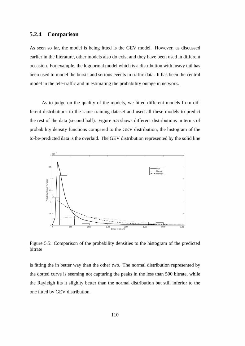
5.2.4 Comparison

As seen so far, the model is being fitted is the GEV model. However, as discussed

earlier in the literature, other models also do exist and they have been used in different

occasion. For example, the lognormal model which is a distribution with heavy tail has

been used to model the bursts and serious events in traffic data. It has been the central

model in the tele-traffic and in estimating the probability outage in network.

As to judge on the quality of the models, we fitted different models from dif-

ferent distributions to the same training dataset and used all these models to predict

the rest of the data (second half). Figure 5.5 shows different distributions in terms of

probability density functions compared to the GEV distribution, the histogram of the

to-be-predicted data is the overlaid. The GEV distributionrepresented by the solid line

0 500 1000 1500 2000 2500 3000 35000

0.5

1

1.5

2

2.5

3x 10

−3

Bitrate in bits unit

Pro

babi

lity

Den

sity

Fun

ctio

n

GEVNormalRayleigh

Figure 5.5: Comparison of the probability densities to the histogram of the predictedbitrate

is fitting the in better way than the other two. The normal distribution represented by

the dotted curve is seeming not capturing the peaks in the less than 500 bitrate, while

the Rayleigh fits it slighlty better than the normal distribution but still inferior to the

one fitted by GEV distribution.

110

In the next few sections, other network QoS parameters are discussed. The ob-

jective is to show modeling results for other QoS parameterslike loss, delay, and jitter

and provide a performance comparison with other frequentlyused models in practice.

5.3 Packet Loss

Packet Loss rate is an important parameter that is included in the design of network

services and QoS specifications. Packet loss is defined as theratio of lost packets to the

total packets transmitted. Packet losses in the Internet are often caused by congestion,

and such losses can be prevented by allocating sufficient bandwidth and buffers for

traffic flows.

The loss rate is due in large to congestion in the network. Congestion in turn

is caused by several factors like the lack of resources such as link bandwidth, queu-

ing resources, processing capabilities, routers memory. However, other causes are also

frequent such as network lower layers errors where packets are dropped due to sig-

nal attenuation in the transmitting media; Network elementfailure such as a router or

switch, however, the time for the network devices to signal the failing router and for

the routing protocol to converge, the packets that were sentto the failing device are

considered lost; loss in application end systems such as buffer over flow.

When packet loss exceeds some accepted level, the application becomes literally

non usable and meaningless. Real time applications such as Internet telephony, video

conferences, and distant surgery subscribe to this kind of applications. This is con-

trasted with the traditional applications such as file transfer or email application where

a delay will not affect much the delivery of the network.

An engineer might want to design the service in such a way thatonly 1 percent

packet loss is tolerated. This calls for high quantile estimation. Using our developed

methodology, the requirement might be that we want to estimate thezp=0.99.

111

As an example of such design request, suppose we have a network such that 1

million connection requests are sent per hour. We are asked to design the network in

such a manner that the traffic loss probability (TLP) is less than 1 percent. That is, out

of 1 million connection requests only at most 10000 connections are lost. Then we are

in the presence of high quantile estimation.

To predict and asses the models, QoS data from university of Napoli are used

for the purpose. The data is packetloss15 from the 10-July folder. Each sample is

calculated using non-overlapping windows of 50ms length. The data are plotted in

Figure 5.6 which shows the two portions of the data, the one known and the other to be

predicted. In the x-axis is the time per 50 milliseconds steps while the vertical or y-axis

0 500 1000 1500 2000 25000

50

100

150

200

250

300

350

400

450

500

time scale in 50 ms

Num

ber

of lo

st p

acke

ts

Figure 5.6: Lossrate plot witht he first portion(1000) indicating the known values, theother portion is supposedly unknown and to be predicted

registers the number of lost packets. It is remarked that there is a cyclical behavior of

the loss in the packet. This cyclical behavior is used as a natural block size with block

size fixed into 50 observations each. The GEV model fitted is thus has the following

parameters(ξ = 0.78(0.3), µ= 77(3.5), σ = 13(4)). Thus the model is fat tailed with

a positive shape parameter which is indication that events far greater than what have

been observed so far are possible.

The unknown part of the data shows clearly that the data are indeed heavy tailed.

The spikes just before the 1500 point in the plot in Figure 5.6confirms this fact. The

return level plot in Figure 5.7 give a further confirmation ofthe heavy tail property

112

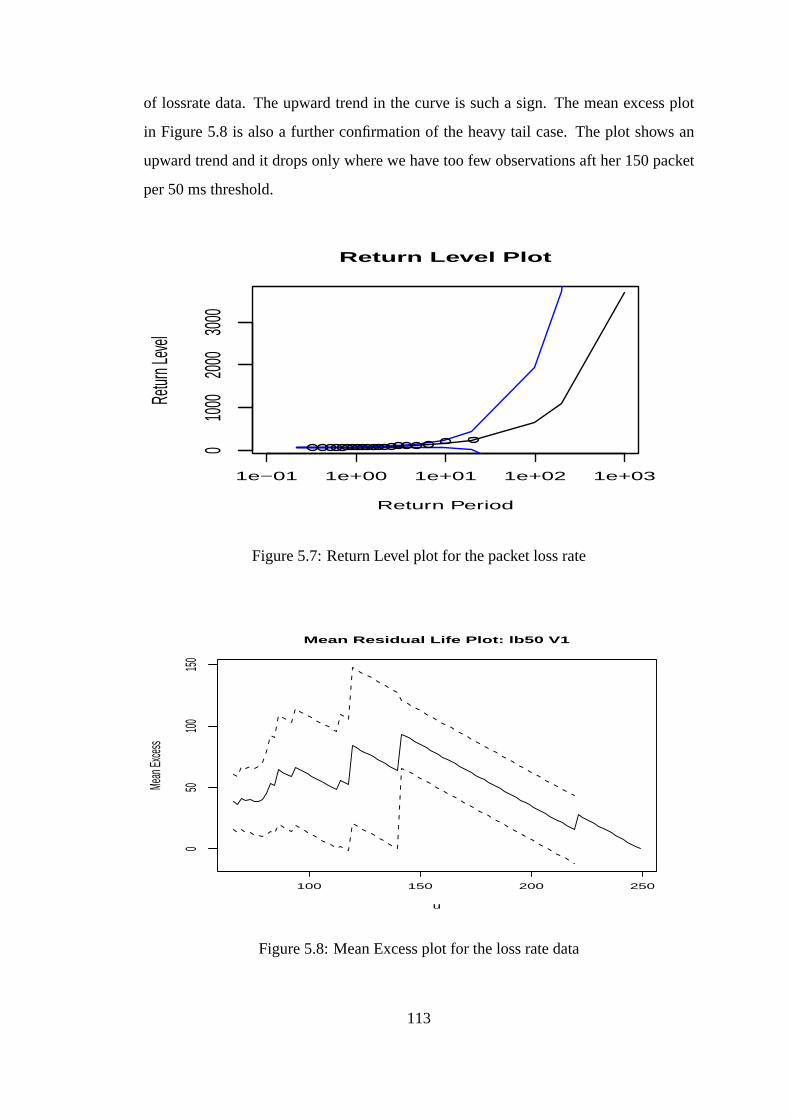
of lossrate data. The upward trend in the curve is such a sign.The mean excess plot

in Figure 5.8 is also a further confirmation of the heavy tail case. The plot shows an

upward trend and it drops only where we have too few observations aft her 150 packet

per 50 ms threshold.

1e−01 1e+00 1e+01 1e+02 1e+03

010

0020

0030

00

Return Period

Retur

n Leve

l

Return Level Plot

Figure 5.7: Return Level plot for the packet loss rate

100 150 200 250

050

100

150

u

Mean

Exce

ss

Mean Residual Life Plot: lb50 V1

Figure 5.8: Mean Excess plot for the loss rate data

113

5.4 Packet Delay

In end to end quality of service measurement, an important quantity is the end to end

per packet delay. Network delay is measured in two ways: one way delay or round

trip delay. The one way delay is the difference between the time the packet received

and the time it has been sent. One way delay is particularly important for non-adaptive

time-critical applications that have a stringent delay requirement to operate correctly.

Examples are the VoIP and Video conferencing. The other typeof delay measurements

is the round trip delay or round trip time (RTT) which denotessimply the two ways

delay, that is the difference between the time the packet is sent and the time it is received

at the other end. Adaptive applications such as data transfer (using TCP) have their

delay defined in terms of the round trip delay.

The delay in network is composed of four components that add up to give the

network delay, propagation delay, switching delay, scheduling delay, serialization de-

lay. Propagation delay is the time the packet takes to travelthe distance between two

end points; it is affected by the distance and the media used and governed by the light

speed. Switching delay is the time the packet spend in a router or a network device

for the processing, it gets smaller with increased router processing power. Scheduling

delay is the time the packet spend waiting in queue both inbound and outbound queues.

The serialization delay is the time taken to clock a packet onto a link. Delay regula-

tion and measurements become particularly important for sensitive application to delay

such as real time applications. However, when networks are designed, there should be

some bounds on the appropriate level of the delay.

For example, in VoIP applications, the concept of playback makes an important

use of extreme measures of delay. Playback is simply a methodusing buffers to reorder

the packets and play them back in the correct sequence. The data arriving before the

playback point are simply stored in a buffer until the playback point comes. Packets

that arrive late are either simply discarded or the playbackpoint is adjusted further. It

is important for such applications to know the extreme measures of the delay and the

114

associated bounds; thus showing the importance of these extreme events in practice.

Figure 5.9 is showing the delay time series obtained from theUniversity of Napoli

Dataset.

0 500 1000 1500 2000 25000

0.05

0.1

0.15

0.2

0.25

0.3

0.35

time in 50 ms steps

Del

ay in

sec

onds

Known Data (1000)

Figure 5.9: Packet delay series

The same steps used in the bitrates earlier are applied here.The model will be

based on the first 1000 data points as indicated in the figure bythe double arrow. The

rest of the data are kept to validate and assess the performance of the prediction based

on the fitted model.

To fit a GPD model, first we de-clustered the data with a threshold of 0.05 and a run

length of 4. The fitted GPD model has its parameters estimatedas(ξ =,0.19(0.2), σ =

0.037(0.01). This model shows that delays are eminent and not bounded, far more de-

lays are possible than what is observed so far. This is true from the positive value of

the shape parameter,ξ, estimates. The mean excess plot is showing an upward curve

which is an indication of the heavy tail of the exceedances, see Figure 5.10. Also we

find closely associated with the delay is the concept of delay-jitter which play an impor-

tant role particularly in some real time applications like voice and video conferencing.

5.4.1 Comparison

Three models that fit the bursts data are compared for the packet delay series. These

models are the nearest fit to the (to be predicted) packet delay data. The densities are

plotted and overlaid on the histogram of the predicted packet delay data, see Figure

115

0.00 0.05 0.10 0.15

0.00

0.05

0.10

0.15

u

Mea

n E

xces

s

Mean Residual Life Plot: delay V1

Figure 5.10: Mean Excess plot for the packet delay dataset

5.11. In this case, the GEV is again showing a superior performance in the prediction

of the unknown packet delay represented by the histogram. The Normal and Rayleigh

densities are still far from the predicted traffic.

5.5 Delay Jitter

Jitter is about the variation in network delay (the difference between the largest and the

smallest delay). Jitter is the variation in one way delay fortwo consecutive packets as

defined by [RFC3393]. Jitter results from the variation in the components of network

delay discussed earlier, namely: propagation delay, switching delay, scheduling delay,

and serialization delay.

In the application level, some are sensitive to delay while the others are less

sensitive to it. In general, applications that use the TCP arenot sensitive to delay-

116

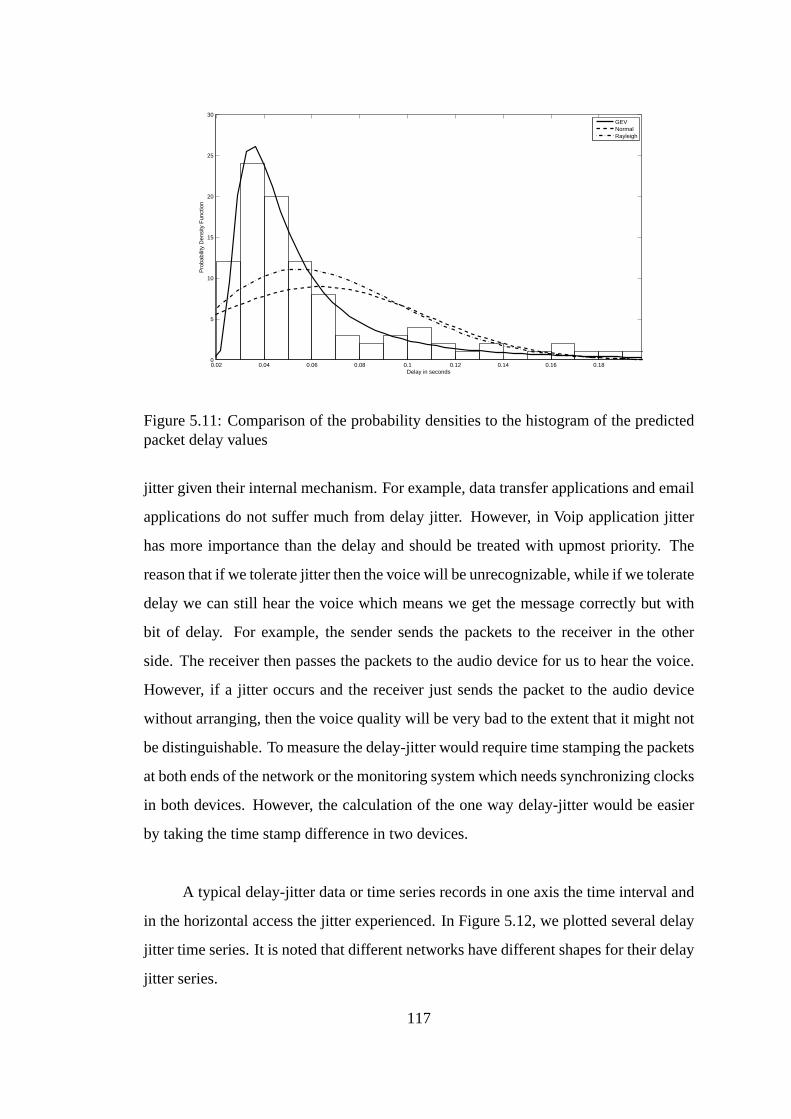
0.02 0.04 0.06 0.08 0.1 0.12 0.14 0.16 0.180

5

10

15

20

25

30

Delay in seconds

Pro

babi

lity

Den

sity

Fun

ctio

n

GEVNormalRayleigh

Figure 5.11: Comparison of the probability densities to the histogram of the predictedpacket delay values

jitter given their internal mechanism. For example, data transfer applications and email

applications do not suffer much from delay jitter. However,in Voip application jitter

has more importance than the delay and should be treated withupmost priority. The

reason that if we tolerate jitter then the voice will be unrecognizable, while if we tolerate

delay we can still hear the voice which means we get the message correctly but with

bit of delay. For example, the sender sends the packets to thereceiver in the other

side. The receiver then passes the packets to the audio device for us to hear the voice.

However, if a jitter occurs and the receiver just sends the packet to the audio device

without arranging, then the voice quality will be very bad tothe extent that it might not

be distinguishable. To measure the delay-jitter would require time stamping the packets

at both ends of the network or the monitoring system which needs synchronizing clocks

in both devices. However, the calculation of the one way delay-jitter would be easier

by taking the time stamp difference in two devices.

A typical delay-jitter data or time series records in one axis the time interval and

in the horizontal access the jitter experienced. In Figure 5.12, we plotted several delay

jitter time series. It is noted that different networks havedifferent shapes for their delay

jitter series.

117

0 500 1000 1500 2000 25000

2

4x 10

−3

0 500 1000 1500 2000 25000

0.5

1x 10

−3

Jitte

r D

elay

in s

econ

ds

0 500 1000 1500 2000 25000

0.5

1x 10

−3

0 500 1000 1500 2000 25000

2

4x 10

−4

time in 50 ms steps

Figure 5.12: Some Delay-Jitter time series

A GPD model was fitted to the jitter series number three in the plot from top to

down. The parameters are given as(ξ = 0.3(0.17), σ = 0.00004(2e−5)). Based on

these parameters, all the prediction tools can be used. For instance, the return level

plot is given by Figure 5.13. The mean excess function is alsodefined accordingly as

discussed in the bitrates case.

5.5.1 Comparison

The delay-jitter or simply the jitter is fitted to a number of probability density models.

Some of them deviated to far from the to-be-predicted traffic. Their densities when

compared to the GEV is less of a fit to the model. In Figure 5.14,the GEV model

is compared to the Lognormal density. The from the figure it isclear that the GEV

model outperform the Lognormal model, however, this is justgraphical, more elaborate

method is thus needed to effectively assess the performanceof the different models.

This will be discussed next.

118

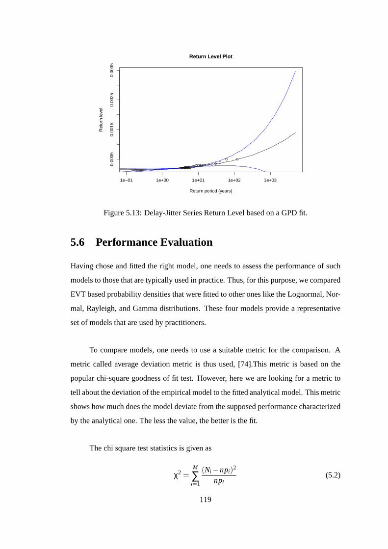
1e−01 1e+00 1e+01 1e+02 1e+03

0.00

050.

0015

0.00

250.

0035

Return Level Plot


Ret

urn

leve

l

Figure 5.13: Delay-Jitter Series Return Level based on a GPD fit.

5.6 Performance Evaluation

Having chose and fitted the right model, one needs to assess the performance of such

models to those that are typically used in practice. Thus, for this purpose, we compared

EVT based probability densities that were fitted to other ones like the Lognormal, Nor-

mal, Rayleigh, and Gamma distributions. These four models provide a representative

set of models that are used by practitioners.

To compare models, one needs to use a suitable metric for the comparison. A

metric called average deviation metric is thus used, [74].This metric is based on the

popular chi-square goodness of fit test. However, here we arelooking for a metric to

tell about the deviation of the empirical model to the fitted analytical model. This metric

shows how much does the model deviate from the supposed performance characterized

by the analytical one. The less the value, the better is the fit.

The chi square test statistics is given as

χ2 =M

∑i=1

(Ni −npi)2

npi(5.2)

119

1 1.5 2 2.5 3 3.5

x 10−4

0

2000

4000

6000

8000

10000

12000

14000

Jitter in seconds

Pro

babi

lity

Den

sity

Fun

ctio

n

GEVLognormal

Figure 5.14: Comparison of two densities that are used to predicted the packet Jitterseries

To apply this test, the distribution is divided into bins, and then the difference between

the number of expected data that falls in particular bin is compared to the actually

falling into that bin. In the above formula, M denotes the number of bins,pi is the

probability of observations falling into theith bin,n is the total number of observations

while Ni is the number of observations that fall in the ith bin exactly. The difficulty

of using chi-square test comes from the fact that it is designed to compare identical

distributions of same size. The value ofChi increase withn which make it difficult

to compare different distributions empirical and analytical ones. Thus, the following

quantity is introduced

K =M

∑i=1

(Ni −npi)2

(npi)2 (5.3)

Note the change in the denominator power. This slight modification makes the test

invariant with the change of values of n. The average deviation metric is then computed

as

µ=√

K2/M (5.4)

120

Table 5.1: Average deviation metric comparisonDataset GEV Lognormal Normal Rayleigh Gamma

Bitrate (ext) 2056.2 3158.6 22900 12924 7686.6Prediction 2372.9 3280.5 31070 6322 4397

Lossrate 46.75 55.5 52.26 44.57 136.17Prediction 21.3800 15.98 23.21 42.85 138.73

Delay 0.9528 0.9137 149.1398 43.8856 1.0830Prediction 0.9807 0.9809 0.9690 0.9717 0.9792

Delay-Jitter 0.9999 0.9996 0.9620 0.9998 0.9983Prediction 1.00 0.9998 0.9489 0.9999 0.9989

For more discussion on this metric, see [74]. This metric is used to compare the EVT

based models fitted to both internal and external traffic in the bitrate case and the other

parameters like loss, delay, and jitter. The comparison will be with the lognormal

distribution which is commonly used for the purpose.

Table 5.1 shows the average deviation metric for the four Quality of Service param-

eters based on the fitted models. As mentioned above, this metric shows how good the

approximation to the analytical models is, where the ability of the prediction is also

shown. For each quality of service parameter we have an entryfor the model based on

the used data, and prediction entry based on the (supposedly) unknown data.

For the all the data, the average deviation metric is computed for the training

data and for the predicted data as well based on the fitted probability density function.

Four frequently used distributions are put into comparisonwith the Extremes model

GEV. For example, in the case of bitrate training data, the GEV model has a slightly

lower deviation metric than the lognormal model; the normalmodel performs the worst.

When it comes to the prediction of the unknown data, the GEV still performs better

than other distributions, with normal distribution performs the least and Rayleigh doing

slightly better. To visualize the entries from the above table, a plot is produced, see

Figure 5.15. In this plot, each column represents a probability density as indicated by

the legend to the right. We did a slight change in the scale in the values of the bitrate

data, this change of scale does not alter the interpretationof the results, it is merely to

visualize the data in comparable scale.

For every QoS parameter, the columns represent the different densities that are fit

121

Figure 5.15: Average deviation metric for the different densities

compared to the GEV distribution. In the case of the bitrate predicted data, the plot

shows that GEV model has the least deviation metric from thanthe other densities. The

loss rate data, we see the GEV has low deviation metric, but the lognormal outperform

it. However, when seen in the fitting to the original data, theGEV outperformed all the

others consistently. The delay and jitter show a very comparable performance by all

the densities. In that case, it is believed the a GPD model based on a threshold would

be more suitable due to the nature of the dat.

The delay rates show a behavior that is dominated by an almostequivalent power

of prediction for the four densities compared to the GEV one.This behavior seems to

be governed by some protocol design issues like the re-transmission in the TCP case;

however, looking into the delay series in Figure 5.9 page 115, it is also remarked that

the delay rates have somehow artificial bound that might verymuch have affected the

behavior of the prediction.

122

The Delay-Jitter parameter is also showing a similar behavior to the delay series

where all the distribution are producing almost similar results for both the prediction

and the fitting values for the average deviation. Only the normal distribution shows a

different behavior and lower average deviation metric for both prediction and fitting.

5.7 Summary

Service Level Agreements are tailored and designed to address different requirements

depending on the application. For example, some applications are sensitive to the bi-

trates; some are for loss rate like real time applications while some are more tolerant

than others. The study is conducted for the four parameters that are widely used for

QoS: Bitrate, Packet Loss, Packet Delay, and Delay-Jitter atthe network level. A proper

quantification of the extreme cases in these quantities is valuable to maintain a well de-

signed quality of service and define robust metrics for Service Level Agreements.

In this Chapter the prediction tools are shown in action and a comparison is made

among popular models such as Lognormal and Gamma densities that are used in prac-

tice. These results show good performance of the EVT based modeling using GEV in

the case of Bitrate and the Packet Loss. For the packet delay, the performance of the

EVT based model is not very different from the others and further adjustment might

then be necessary to unleash the model prediction capabilities. These methods are ap-

plicable both for the network level QoS and for the applications level as well.

123

CHAPTER 6

CONCLUSION

Modeling bursts and serious deteriorations in the traffic iscritical for the contin-

uous growth of Internet while maintaining an adequate quality of service for the users.

In this work bursts and serious deteriorations in Internet questions are addressed by

using Extreme Value Theory. A clear methodology is developed for some applications

of Extreme Value methods.

Quality of Service parameters that are commonly used in service level agree-

ments are modeled and predicted using EVT. These parametersare bitrate, packet loss,

delay, and jitter. Extreme measures are thus developed using extreme value theory,

namely probability distributions of bursts, their return level, and return period.

The extreme value tools are applied with care and by taking all the preliminary

steps towards a successful implementation through detailed exploratory data analysis.

It takes place before any model fitting exercise. This was followed with diagnostics and

model checking techniques based on graphical assessment tools. These steps are carried

out for the three models that are applied in EVT, namely Block Maxima Modeling

through a GEV distribution, Peaks Over Threshold modeling through a Generalized

Pareto Distribution, andr-Largest Order Statistics.

The first model fitted is the Generalized Extreme Value model based on the Block

Maxima methodology. This is the classical modeling in Extreme Value Theory. The

internal traffic of both simulated and Belcore traces were shown to fall in the domain of

attraction of Weibull distribution with possibilities of being in the domain of attraction

of Gumbel distribution as well. This is equivalent to sayingthat bursts from internal

traces followed GEV distribution with parameters ranging from zero (Gumbel) to the

negative values (Weibull). This model for the burst and serious deteriorations in internal

traffic means bursts and serious deteriorations in traffic follow a distribution that is

bounded from above and cannot exceed certain values. This can be explained by the

very nature of internal traffic. In LAN settings, the set of applications is finite and they

have a finite set of demonstrated behavior.

On the other hand, external traffic traces were modeled usinga GEV distribution

with a positive shape parameter which means that external traces fall in the domain of

attraction of Frechet distribution. Frechet is a heavy taildistribution which means also

that external traffic have spikes and serious deteriorations are frequent. That shows the

importance of having appropriate measures for these quantities. The GEV modeling is

fine-tuned by including the external index parameter that isdesigned to account for the

dependency structure in the data. It should be clear by now that EVT was designed for

independent data case.

Secondly, Peaks Over Threshold model was used for the prediction. POT mod-

eling has presented its own point of view of the prediction issue. Considering a suffi-

ciently high threshold, GPD distribution was fitted to both internal and external traces.

The internal fitting gave rise to GPD with negative shape parameters while external

traffic gave a positive GP distribution shape parameter. These observations are in ac-

cordance with those found using the GEV BM methodology. POT has encountered its

own challenges because of the clustering of extremes. Thus,a de-clustering scheme

was necessary so that Maximum Likelihood estimation would be valid.

The third and last model in the Extreme Value Theory is the−r largest order

statistics (RLOS) model. It was also fitted to a different sample for traffic trace. It

is shown that RLOS have indeed brought in an improvement in theaccuracy of the

parameter compared to the GEV. However, the diagnostics plots showed that the fit was

not particularly good. This model will be subjected to more investigation especially

concerning the stationary assumption of the data.

126

These findings have many implications to the QoS in the Internet and other appli-

cations. The need for a robust QoS metrics in mission critical applications is thus met.

These applications range from medical field to the military one. Including new robust

metrics based on the bursts fitted model will leave both usershappy for the service they

receive. Service Providers (ISPs) will be able to use their valuable resources in the most

efficient way. The complexity of the processing of the modelsmakes it very efficient

in terms of memory use and processing power. The models traditionally used for the

purpose rely on the whole data set to be fed into the model. However, in this case we

need only subsets of the data to work on, either the block maxima or exceedances. This

will make it possible for an on line implementation of our model.

However, Internet today is a very changing and hectic environment that needs a

lot of research and attention. Due to its changing behavior,any research project that

would take too long will have no applicability by the time it is done. When is the last

time somebody used Netscape navigator? Windows 98? or even adial-up connection?.

Analytical modeling by its very nature takes time to developand to produce mathemat-

ically sound and tractable models. Due to such and the like constraints, the study was

limited to readily available data from the Belcore laboratories and from the University

of Napoli Traces as conducting a large scale testing was not feasible.

Taking data from Belcore to base the research on would be dangerous at first

sight since the Internet is changing very rapidly. However,after careful consideration,

the data still represent what is happening now in the Internet. It is bursty, self-similar,

long range dependent and fractal. Its high quality is still appealing to many researchers

and publications. This decision have also been validated bysome simulated Internet

traffic data based on the fractional Brownian motion, and the linear fractional alpha

table motion. This study should be applicable to other data set and that would be left

for future work.

As this research straddles tools from probability, statistics, and extreme value

with Internet and computer networks, accuracy and rigor have been practiced. However,

perfection becomes an elusive target to pursue. In the following, a summary of the main

127

contributions without repetitions is presented. Directions to future work are presented

next.

1. Bursts and serious deteriorations are modeled and predicted using mainly three

EVT based models.

2. QoS metrics are proposed using Return Level and Return Period to be included

in future Service Level Agreements.

3. A methodology is clearly developed which is less prone to errors.

4. The behavior of Queue buffer fed by a WAN traffic is shown to behave as Frechet

distribution, in contrast to Norros finding for a Queue fed with LAN traffic which

behaves as Weibull.

6.1 Future directions

Although this thesis brings a lot of insight into the bursts and serious deteriorations

in the traffic from the extreme value perspective, a lot more work can still be done

from both theoretical and application points of view. Here some of these directions are

itemized.

• Extending this work by applying the same method to other network parameters

and time series such as Delays, Jitter, Connection Duration,Round Time Trip.

• Extremal Dependency is also another case in hand, using somemultivariate anal-

ysis, the effect of extremes from some parameters can induceextreme in other

time series as well. This study needs a large deployment of traffic measurement

tools to truly study the effect from different angles.

• Other EVT based method like the recentr-largest order statistics are to be inves-

tigated and applied. The selection of the block sizes in the BMmethod and its

effect is also an object of further investigations and research.

• Other directions is on analytical study of the behavior of a buffer fed by a linear

fractional stable noise the type of the external traffic is also to be investigated, this

128

is similar to the Norros results for the buffer behavior whenit is fed by fractional

Gaussian noise, the typical model for the internal traffic.

6.2 Publications

• Abdelmahamoud YD, Abas Md Said, and Halabi Bin Hasbullah, ”Application

of Extreme Value Theory to Bursts Prediction”, Signal Processing International

Journal, vol.3 (4), 2010.

• Abdelmahamoud YD, Abas Md Said, and Halabi Bin Hasbullah, ”Predicting

Traffic Bursts Using Extreme Value Theory”, International Conference on Signal

Acquisition and Processing, pp 229-233, IEEE Xplorer 2009.

• Abdelmahamoud YD, Abas Md Said, and Halabi Bin Hasbullah, ”Quality of

Service using Generalized Pareto Distribution”, ITSIM 2010.

• Abdelmahamoud YD, Abas Md Said, and Halabi Bin Hasbullah, ”Predicting In-

ternal LAN Bursts using Extreme Value Theory”, National Postgraduate Confer-

ence, 2009.

• Abdelmahamoud YD, Abas Md Said, and Halabi Bin Hasbullah, ”r-largest order

statistics for the prediction of bursts and serious deteriorations in network traffic”,

International Conference on Computer and Communication Devices, Indonesia

2011.

129

REFERENCES

[1] P. Abry. Wavelet analysis of long-range-dependent traffic. IEEE Transactionson Information Theory, 44(1):2–15, 1998.

[2] Patrice Abry and Fabrice Sellan. The wavelet-based synthesis for fractionalbrownian motion proposed by f. sellan and y. meyer: Remarks and fast im-plementation.Applied and Computational Harmonic Analysis, 3(4):377 – 383,1996.

[3] J. M. P. Albin. On extremal theory for self-similar processes.Annal of Proba-bility, 26(2):743–793, Feb 1998.

[4] J. M. P. Albin. Extremes of totally skewed [alpha]-stable processes.StochasticProcesses and their Applications, 79(2):185–212, Feb 1999.

[5] Martin F. Arlitt and Carey L. Williamson. Web server workload characterization:the search for invariants.SIGMETRICS Perform. Eval. Rev., 24(1):126–137,1996.

[6] F. Baker, K. Chan, and A. Smith. Management information base for the differ-entiated services architecture, 2002.

[7] Jerry Banks, John Carson, Barry L. Nelson, and David Nicol.Discrete-EventSystem Simulation (4th Edition). Prentice Hall, 4 edition, December 2004.

[8] Jan Beirlant, Yuri Goegebeur, Johan Segers, and Jozef Teugels. Statistics ofExtremes Theory and Applications. WILEY, England, 2004.

[9] SIDNEY I. RESNICK BERNARDO D’AURIA. Data network models of bursti-ness.Advances in Applied Probability, 38(2):373–404, 2006.

[10] Robert M. Bethea and R. Russell Rhinehart.Applied Engineering Statistics(Statistics: A Series of Textbooks and Monographs). CRC Press, 1 edition, Au-gust 1991.

[11] S. Blake, D. Black, M. Carlson, E. Davies, Z. Wang, and W. Weiss. An architec-ture for differentiated service. 1998.

[12] R. Braden, D. Clark, and S. Shenker. Integrated services inthe internet architec-ture: an overview. 1994.

[13] T Braun, m Diaz, J.E Gabeiras, and Th. Staub.End-to-End Quality of ServiceOver Heterogeneous Networks. Springer, New York, NY, USA, 2008.

131

[14] B.V.Gnedenko. Sur la distribution limite du terme de maximum d’une seriealeatoire.Ann. Math., 44:423–453, 1943.

[15] D.O. Cajueiro and B.M. Tabak. The rescaled variance statistic and the deter-mination of the hurst exponent.Mathematics and Computers in Simulation,70(3):172–179, 2005.

[16] B. Canberk and S. Oktug. Self similarity analysis and modeling of voip trafficunderwireless heterogeneous network environment. pages 76–82, 2009.

[17] Jin Cao, William S. Cleveland, Dong Lin, and Don X. Sun. Internet traffic tendsto poisson and independent as the load increases. Technicalreport, 2001.

[18] G. Carl, R.R. Brooks, and S. Rai. Wavelet based denial-of-service detection.Computers and Security, 25(8):600–615, 2006.

[19] Enrique Castillo, Ali S. Hadi, N. Balakrishnan, and Jose Maria Sarabia.ExtremeValue and Related Models with Applications in Engineering and Science. Wiley,Wiley, 2004.

[20] H. Jonathan Chao and Xiaolei Guo.Quality of Service Control in High-SpeedNetworks. John Wiley & Sons, Inc., New York, NY, USA, 2001.

[21] Stuart Coles. An Introduction to Statistical Modeling of Extreme Values.Springer-Verlag, 2001.

[22] Graham Cormode. What is new: Finding significant differences in network datastreams. Inin Proc. of IEEE Infocom, pages 1534–1545, 2004.

[23] Mark E. Crovella and Azer Bestavros. Self-similarity in world wide web traffic:evidence and possible causes.IEEE/ACM Trans. Netw., 5(6):835–846, 1997.

[24] A. C. Davison and R. L. Smith. Models for exceedances over high thresholds.Journal of the Royal Statistical Soceity. Series B, 52(3):393–442, 1990.

[25] L. de Haan. On regular variation and its application to the weak convergence ofsample extremes.Mathematical Centre Tracts, 32, pages 123–124, 1970.

[26] A.B. Downey. Evidence for long-tailed distributions inthe internet.Proceedingsof the ACM SIGCOMM Internet Measurement Workshop, pages 229–241, 2001.

[27] D. J. Dupuis. Extreme value theory based on the r largestannual events: a robustapproach.Journal of Hydrology, 200(1-4):295 – 306, 1997.

[28] P. Embrechts and M. Maejima. An introduction to the theory of self-similarstochastic processes.International Journal of Modern Physics B, 14(12-13):1399–1420, 2000.

[29] Paul Embrechts, Thomas Mikosch, and Claudia Kluppelberg. Modelling Ex-tremal Events: for Insurance and Finance. Springer-Verlag, London, UK, 1997.

132

[30] Agner K. Erlang. The theory of probabilities and telephone conversations.NytTidsskrift for Matematik, 20(B):33–39, 1909.

[31] John William Evans and Clarence Filsfils.Deploying IP and MPLS QoS forMultiservice Networks: Theory & Practice. Morgan Kaufmann Publishers Inc.,San Francisco, CA, USA, 2007.

[32] Laura Feinstein and Dan Schnackenberg. Statistical approaches to ddos attackdetection and response. InIn Proceedings of the DARPA Information Survivabil-ity Conference and Exposition, pages 303–314, 2003.

[33] A. Feldmann, A.C. Gilbert, and W. Willinger. Data networks as cascades: Inves-tigating the multifractal nature of internet wan traffic. volume 28, pages 42–55,1998.

[34] Baerbel Finkenstaedt and holger Rootzen.Extreme Values in Finance, Telecom-munications and the Environment. CRC Press, 2004.

[35] Hans Fischer.A History of the Central Limit Theorem: From Classical to Mod-ern Probability Theory. Springer, 2010.

[36] R A Fisher and L HC Tippett. On the estimation of the frequency distributions ofthe largest or smallest member of a sample.Proc. Cambridge phil. soc., 24:180–190, 1928.

[37] R.A. Fisher and L. H. C. Tippett. Limiting forms of the frequency distribution ofthe largest and smallest member of a sample.Proc. of the Cambridge Philosph-ical Society, 24:180–190, 1928.

[38] Frechet. Sur la loi de probabilit de l’cart maximum.Annales de la Socit Polon-aise de Mathematique, 6:93–116, 1927.

[39] Mark W. Garrett and Walter Willinger. Analysis, modeling and generation ofself-similar vbr video traffic.SIGCOMM Comput. Commun. Rev., 24(4):269–280, 1994.

[40] P. Pablo Garrido, Manuel P. Malumbres, and Carlos T. Calafate. ns-2 vs. opnet:a comparative study of the ieee 802.11e technology on manet environments. InProceedings of the 1st international conference on Simulation tools and tech-niques for communications, networks and systems & workshops, Simutools ’08,pages 37:1–37:10, ICST, Brussels, Belgium, Belgium, 2008. ICST (Institute forComputer Sciences, Social-Informatics and Telecommunications Engineering).

[41] Roger L. Berger George Casella.Statistical Inference. Duxbury, Pacific Grove,CA 93950, USA, 2001.

[42] E. J. Gumbel. Les valeurs extrmes des distributions statistiques. Annales del’Institut Henri Poincar, 4(2):115–158, 1935.

[43] E. J. Gumbel. The return period of flood flows.The Annals of MathematicalStatistics, 12:163–190, 1941.

133

[44] E.J. Gumbel.Statistics of extremes. Dover books on mathematics. Dover Publi-cations, 2004.

[45] James D. Hamilton.Time Series Analysis. Princeton University Press, 1 edition,January 1994.

[46] R. I. Harris. Gumbel re-visited - a new look at extreme value statistics applied towind speeds.Journal of Wind Engineering and Industrial Aerodynamics, 59(1):1– 22, 1996.

[47] Jain, Raj, Routhier, and Shawn A. Packet trains - measurements and a new modelfor computer network traffic.IEEE Journal on Selected Areas in Communica-tions, SAC-4(6):986–995, 1986.

[48] Murad S. Taqqu Jan Beran, Robert Sherman and Walter Willinger. Long-rangedependence in variable-bit-rate video traffic.IEEE Transactions on Communi-cation, 43(234):1566–1579, 1995.

[49] Yuming Jiang, Chen-Khong Tham, and Chi-Chung Ko. Challenges and ap-proaches in providing qos monitoring.Int. J. Netw. Manag., 10:323–334,November 2000.

[50] Norman L. Johnson, Samuel Kotz, and N. Balakrishnan.Continuous UnivariateDistributions, Vol2. Wiley, 1995.

[51] A. Karasaridis and D. Hatzinakos. Network heavy trafficmodeling usingalpha-stable self-similar processes.Communications, IEEE Transactions on,49(7):1203–1214, Jul 2001.

[52] S. Kato and T. Osogami. Evaluating availability under quasi-heavy-tailed repairtimes. pages 442–451, 2008.

[53] Richard W. Katz, Marc B. Parlange, and Philippe Naveau. Abstract statistics ofextremes in hydrology, 2002.

[54] Jon Kleinberg. Bursty and hierarchical structure in streams, 2002.

[55] V. P. Kumar, T. V. Lakshman, and D. Stiliadis. Beyond besteffort: Router archi-tectures for the differentiated services of tomorrow’s internet. IEEE Communi-cations Magazine, 36:152–164, 1998.

[56] M. R. Leadbetter. On a basis for [‘]peaks over threshold’modeling.Statistics &Probability Letters, 12(4):357–362, October 1991.

[57] M. R. Leadbetter and Holger Rootzen. Extremal theory for stochastic processes.The Annals of Probability, 16(2):431 – 478, 1988.

[58] Will E. Leland, Murad S. Taqqu, Walter Willinger, and Daniel V. Wilson. Onthe self-similar nature of ethernet traffic (extended version). IEEE/ACM Trans.Netw., 2(1):1–15, 1994.

134

[59] L. Li and G. Lee. Ddos attack detection and wavelets.Telecommunication Sys-tems, 28(3-4):435–451, 2005.

[60] Chunfeng Liu, Yantai Shu, Jiakun Liu, and O.W.W. Yang. Application of ex-treme value theory to the analysis of wireless network traffic. In Communica-tions, 2007. ICC ’07. IEEE International Conference on, pages 486–491, June2007.

[61] Gilberto Flores Lucio, Marcos Paredes-farrera, Emmanuel Jammeh, MartinFleury, and Martin J. Reed. Opnet modeler and ns-2: Comparing the accuracyof network simulators for packet-level analysis using a network testbed. InIn3rd WEAS International Conference on Simulation, Modellingand OptimizationICOSMO, pages 700–707, 2003.

[62] Stphane Mallat.A Wavelet Tour of Signal Processing, Third Edition: The SparseWay. Academic Press, 3rd edition, 2008.

[63] Benoit Mandelbrot. linktionary.com/b/burst.

[64] Benoit Mandelbrot. Long-run linearity, locally gaussian process, h-spectra andinfinite variances. International Economic Review, 10(1):82–111, February1969.

[65] Krishanu Maulik, Sidney Resnick, Holger, and Rootz ?n. Asymptotic indepen-dence and a network traffic model.Journal of Applied Probability, 2002:671–699, 2002.

[66] J. Mirkovic and P. Reiher. A taxonomy of ddos attack and ddos defense mecha-nisms. volume 34, pages 39–53, 2004.

[67] Claudia Neves and Isabel Fraga Alves. The ratio of maximum to the sum fortesting super heavy tails.Advances in Mathematical and Statistical Modeling,2007.

[68] Claudia Neves and M.Isabel Fraga Alves. Testing extreme valueconditions – anoverview and recent approaches.REVSTAT, 6(1):83–100, 2008.

[69] K. Nichols, S. Blake, F. Baker, and D. Black. Definition of the differentiatedservices field (ds field) in the ipv4 and ipv6 headers. 1998.

[70] Ilkka Norros. On the use of fractional brownian motion in the theory of con-nectionless networks.IEEE Journal of Selected Areas in Communications,13(6):953–962, 1995.

[71] G. L. O’Brien. A limit theorem for sample maxima and heavybranches in galton-watson trees.Journal of Applied Probability, 17(2):539–545, 1980.

[72] University of Napoli. Quality of service traces.http://www.grid.unina.it/Traffic/index.php, May 2011.

135

http://www.grid.unina.it/Traffic/index.php

[73] Kihong Park, Gitae Kim, and Mark Crovella. On the relationship between filesizes, transport protocols, and self-similar network traffic. pages 171–180, 1996.

[74] Vern Paxson.Empirically Derived Analytic Models of Wide Area Tcp Connec-tions : Extended Report. June 1993.

[75] Vern Paxson and Sally Floyd. Wide-area traffic: the failure of poisson modeling.In SIGCOMM ’94: Proceedings of the conference on Communicationsarchitec-tures, protocols and applications, pages 257–268, New York, NY, USA, 1994.ACM.

[76] P. Pragtong, K.M. Ahmed, and T.J. Erke. Analysis and modeling of voice overip traffic in the real network.IEICE Transactions on Information and Systems,E89-D(12):2886–2896, 2006. cited By (since 1996) 3.

[77] X. Ren, R. Wang, H. Wang, and J. Li. Wavelet choice for detection of ddosattack based on self-similar testing.Nanjing Hangkong Hangtian Daxue Xue-bao/Journal of Nanjing University of Aeronautics and Astronautics, 39(5):588–592, 2007.

[78] Sidney Resnick, Holger Rootz?n, Holger, and Rootz En. Self-similar communi-cation models and very heavy tails. 1998.

[79] Sidney I. Resnick. Heavy tail modeling and teletraffic data. Annals of Statistics,25:1805–1869, 1997.

[80] Sidney I. Resnick.Heavy-Tail Phenomena: Probabilistic and Statistical Model-ing. Springer, USA, 2006.

[81] K.M. Rezaul and V. Grout. Towards finding efficient tools for measuring thetail index and intensity of long-range dependent network traffic. pages 973–980,2007.

[82] R.H. Riedi, M.S. Grouse, V.J. Ribeiro, and R.G. Baraniuk. A multifractalwavelet model with application to network traffic.IEEE Transactions on In-formation Theory, 45(3):992–1018, 1999.

[83] Christian Y. Robert, Johan Segers, and Christopher A.T. Ferro. A sliding blocksestimator for the extremal index.Electronic Journal of Statistics, 3:993–1020,2009.

[84] Z. Sahinoglu and S. Tekinay. On multimedia networks: Self-similar traffic andnetwork performance. 37(1):48–52, 1999.

[85] Gennady Samorodnitsky and Murad S. Taqqu.Stable Non-Gaussian RandomProcesses: Stochastic Models with Infinite Variance. Chapman & Hall, LondonSE1 8HN, 1994.

[86] R. L. Smith. Maximum likelihood estimation in a class of non-regular cases.Biometrica, 72:67–90, 1985.

136

[87] R. L. Smith. Extreme value theory.Handbook of Applicable Mathematics, sup-plement, pages 437–472, 1990.

[88] R.L. Smith. Maximum likelihood estimation in a class of nonregular cases.Biometrika, 72:76–90, 1985.

[89] Stilian Stoev and Murad S. Taqqu. Simulation methods for linear fractionalstable motion and farima using the fast fourier transform.Fractals, 12:2004,2004.

[90] Balachander Krishnamurthy Subhabrata, Er Krishnamurthy, Subhabrata Sen,Yin Zhang, and Yan Chen. Sketch-based change detection: Methods, evalua-tion, and applications. InIn Internet Measurement Conference, pages 234–247,2003.

[91] Nassim Nicholas Taleb.The Black Swan: The Impact of the Highly Improbable.Ranbdom House, 2007.

[92] M.S. Taqqu, V. Teverovsky, and W. Willinger. Is networktraffic self-similar ormultifractal? Fractals, 5(1):63–73, 1997.

[93] John W Tukey.Exploratory Data Analysis. Addison Wesley, 1977.

[94] Masato UCHIDA. Traffic data analysis based on extreme value theory and itsapplications to predicting unknown serious deterioration. IEICE transactions oninformation and systems, 87(12):2654–2664, 20041201.

[95] D. Veitch, N. Hohn, and P. Abry. Multifractality in tcp/ip traffic: The caseagainst.Computer Networks, 48(3):293–313, 2005.

[96] Zheng Wang.Internet QoS: Architectures and Mechanisms for Quality of Ser-vice. Morgan Kaufmann Publishers Inc., San Francisco, CA, USA, 1st edition,2001.

[97] W. Weibull. A statistical theory of the strength of material. Proceedings of RoyalSwedish Academy of Engineering Science, 151:5–44, 1939.

[98] Ishay Weissman. On location and scale functions of a class of limiting processeswith application to extreme value theory.Annals of Probability, 3:178–181,1975.

[99] Ishay Weissman. Estimation of parameters and larger quantiles based onthe k largest observations.Journal of the American Statistical Association,73(364):812–815, 1978.

[100] Walter Willinger and Vern Paxson. Where mathematics meets the internet.No-tices of the American Mathematical Society, pages 961–970, 1998.

[101] Walter Willinger, Vern Paxson, and Murad S. Taqqu. Self-similarity and heavytails: structural modeling of network traffic. pages 27–53,1998.

137

[102] Walter Willinger, Murad S. Taqqu, Robert Sherman, and Daniel V. Wilson. Self-similarity through high-variability: statistical analysis of ethernet lan traffic atthe source level.SIGCOMM Comput. Commun. Rev., 25(4):100–113, 1995.

[103] Y. Xinyu, S. Yi, Z. Ming, and Z. Rui. A novel method of network burst trafficreal-time prediction based on decomposition. volume 3420,pages 784–793,2005.

[104] J. Yan, R Kowalczyk, J. Lin, M.B. Chhetri, S.K. Goh, and J.Zhang. Autonomousservice level agreement negotiation for service composition provision. FutureGeneration Computer Systems, 23(6):748–759, 2007.

[105] M h YANG and R c WANG. Ddos detection based on wavelet kernel supportvector machine.Journal of China Universities of Posts and Telecommunications,15(3):59–63, 2008.

[106] X. Yang, G. Hou, and S. Yang. Ddos attacks detecting algorithm based on con-tinuous wavelet transforms with reliability evaluation.Hsi-An Chiao Tung TaHsueh/Journal of Xi’an Jiaotong University, 42(8):936–939, 2008.

[107] X. Yang, Y. Liu, M. Zeng, and Y. Shi. A novel ddos attack detecting algorithmbased on the continuous wavelet transform.Lecture Notes in Computer Science(including subseries Lecture Notes in Artificial Intelligence and Lecture Notes inBioinformatics), 3309:173–181, 2004.

[108] Lixia Zhang, Steve Deering, Deborah Estrin, Scott Shenker, and Daniel Zappala.Rsvp: A new resource reservation protocol.IEEE NETWORKS MAGAZINE,pages 8–18, 1993.

[109] Xin Zhang and Dennis Shasha. Better burst detection. InProceedings of the22nd International Conference on Data Engineering, ICDE ’06, pages 146–,Washington, DC, USA, 2006. IEEE Computer Society.

[110] A. Zhou, S. Qin, and W. Qian. Adaptively detecting aggregation bursts in datastreams. volume 3453, pages 435–446, 2005.

[111] Yunyue Zhu and Dennis Shasha. Efficient elastic burst detection in data streams.In KDD ’03: Proceedings of the ninth ACM SIGKDD international conferenceon Knowledge discovery and data mining, pages 336–345, New York, NY, USA,2003. ACM.

1

138

extreme value theory i abdelmahamoud youssuf …

Documents